Optimizing YOLOv7 for Semiconductor Defect Detection

Abstract

The field of object detection using Deep Learning (DL) is constantly evolving with many new techniques and models being proposed. YOLOv7 is a state-of-the-art object detector based on the YOLO family of models which have become popular for industrial applications. One such possible application domain can be semiconductor defect inspection. The performance of any machine learning model depends on its hyperparameters. Furthermore, combining predictions of one or more models in different ways can also affect performance. In this research, we experiment with YOLOv7, a recently proposed, state-of-the-art object detector, by training and evaluating models with different hyperparameters to investigate which ones improve performance in terms of detection precision for semiconductor line space pattern defects. The base YOLOv7 model with default hyperparameters and Non Maximum Suppression (NMS) prediction combining outperforms all RetinaNet models from previous work in terms of mean Average Precision (mAP). We find that vertically flipping images randomly during training yields a 3% improvement in the mean AP of all defect classes. Other hyperparameter values improved AP only for certain classes compared to the default model. Combining models that achieve the best AP for different defect classes was found to be an effective ensembling strategy. Combining predictions from ensembles using Weighted Box Fusion (WBF) prediction gave the best performance. The best ensemble with WBF improved on the mAP of the default model by 10%.

1 Introduction

Automatic defect inspection is important for high-yield and reduced engineering time/cost. Techniques such as scanning electron microscopy (SEM) can produce high-resolution images for inspecting defects at the nanometer scale. The inherently noisy nature of SEM images and continuous transitions to smaller nodes causes traditional, rule-based image processing methods for defect inspection to fail [1]. This has spurred interest in machine learning, particularly deep learning (DL), methods that are able to handle noise and changes in scale better [2, 3, 4, 1, 5, 6].

In this study, we focus on defect detection, which involves localizing and classifying defect instances, in SEM images. Dey et al.[1] showed that a DL framework based on RetinaNet detects semiconductor defects more robustly than rule-based image processing techniques. DL-based object detection is a very popular research topic with new techniques and models being proposed constantly. YOLOv7[7] is a state-of-the-art DL-based object detection model based on the YOLO[8] family of models which have become popular for industrial applications.

This study shows that the base YOLOv7 model architecture with default hyperparameters outperforms multiple RetinaNet models. To improve detection performance, many YOLOv7 models with different hyperparameters are systematically trained and evaluated. Furthermore, two detection prediction combination techniques, Non-Maximum Suppression (NMS) and Weighted Box Fusion (WBF), with different model ensemble strategies are compared. The findings from these experiments provide practical insights for DL-based object detection for semiconductor defect detection.

2 Dataset

A collection of 1324 SEM wafer after-developing-inspection images with 3265 defect instances from Dey et al. [1] is reused in this study. The images are of line space patterns with line collapse, gap, probable gap (or p-gap), bridge, or microbridge defects. Examples of each of these five defect types are shown in Figure 1. Table 1 shows statistics of the dataset including the number of images and defect instances in the train, validation, and test splits.

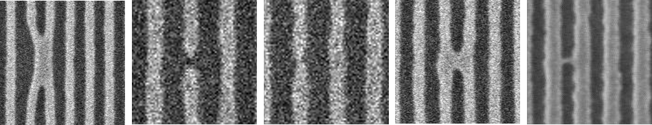
Figure 1: Examples of (from left to right) line collapse, gap, probable gap, bridge, and microbridge line space pattern defects.

Table 1: SEM image dataset statistics for each split.

Sample counts	Train	Validation	Test
Line collapse	550	66	76
Bridge	238	19	17
Microbridge	380	47	78
Gap	1046	156	174
Probable Gap	315	49	54
Total instances	2529	337	399
Total images	1053	117	154

3 Methodology

First, the YOLOv7[7] base model was trained using the default hyperparameters. Hyperparameters that were hypothesized to noticeably affect the detection performance of the model were chosen for experimentation. These can be categorized as either “weights & learning” or “data augmentation” hyperparameters. The former affects the number of weights of the model or how they are updated. The latter modifies the input images during training. The models were trained so that one of these hyperparameters had been assigned a value different from that of its default value. The hyperparameters and the default and modified values are shown in Table 2. Examples of images after applying each of the chosen data augmentations operations are shown in Figure 2.

Table 2: Hyperparameters selected for experimentation with their default and chosen modified values.

Type	Hyperparameter	Default	Modified (1)	Modified (2)
Weights & learning	Anchor threshold	4	9	13
	Number of anchors	3	9	13
	IOU threshold	0.2	0.5	0.75
	Object loss gain	0.7	0.25	0.5
	Class loss gain	0.3	0.1	0.5
	Box loss gain	0.05	0.1	0.25
	Focal-loss gamma	0.0	1.0	1.5
	Freeze backbone layers	First layer only	First 25 layers	All 50 layers
	Model size	Base	Tiny	Base-X
Data augmentation	Vertical flipping (probability)	0.0	0.5	-
	Horizontal flipping (probability)	0.5	0.0	-
	Mosaic[9]	1.0	0.0	0.5
	Scale (+/- gain)	0.5	0.25	0.75
	Translation (+/- fraction)	0.2	0.0	0.5
	Angle (+/- degrees)	0	45	90
	Shear (+/- degrees)	0	15	30
	HSV (fraction)	0.015/0.7/0.4 (h/s/v)	0.0 (all)	1.0 (all)

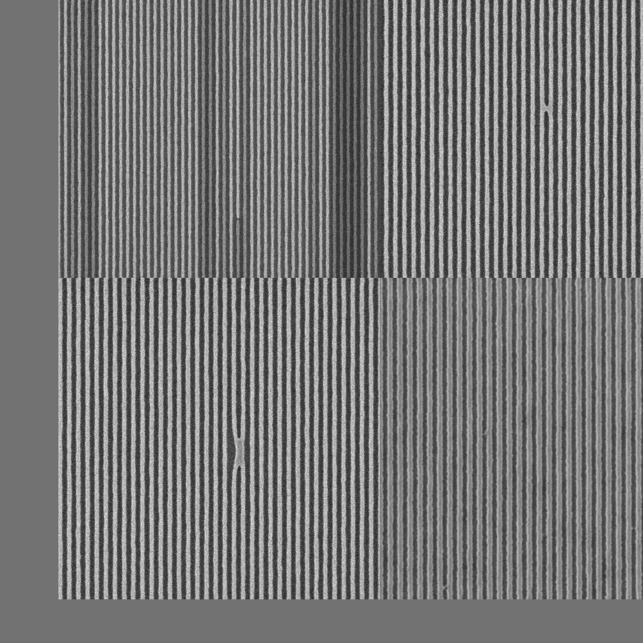
(a) Mosaic[9]

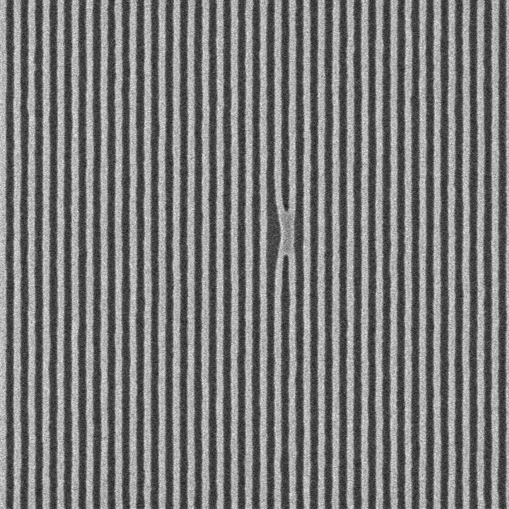
(b) Vertical flip

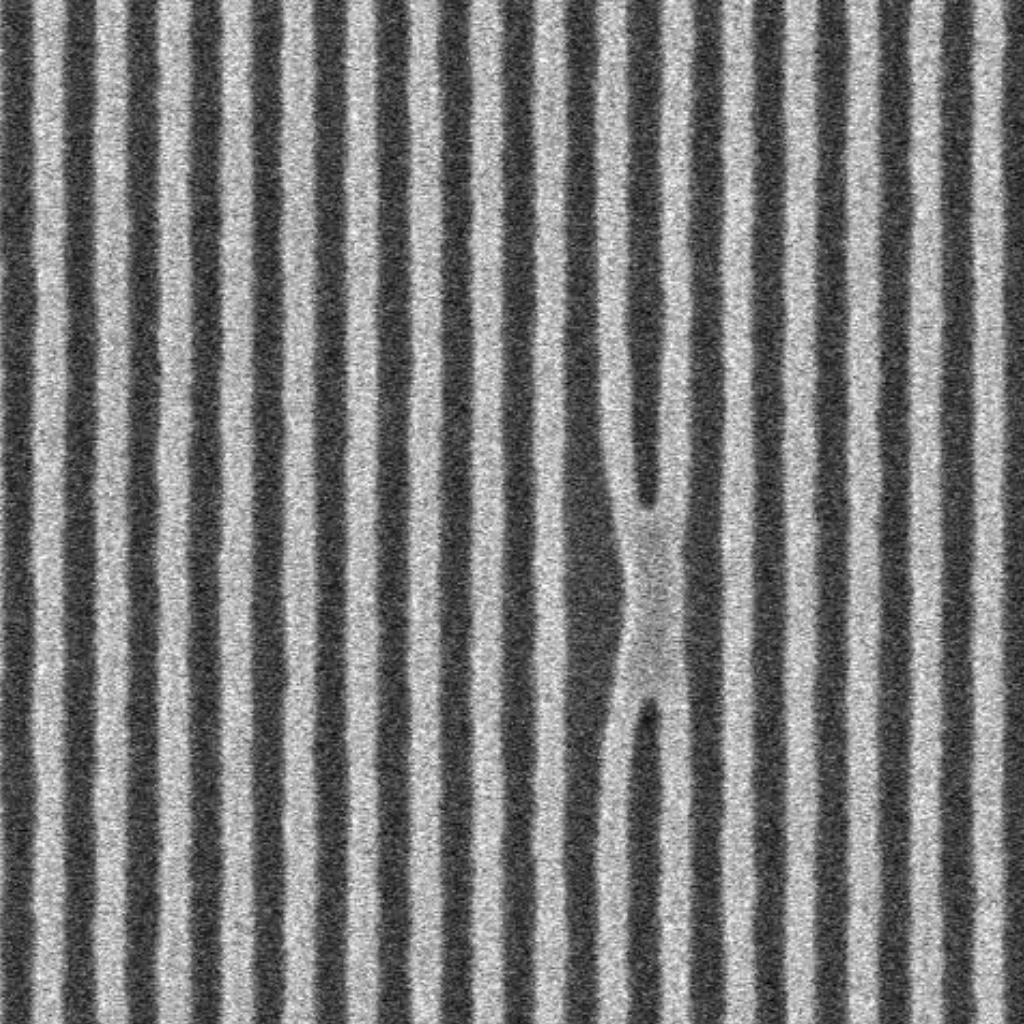
(c) Scale (+0.15)

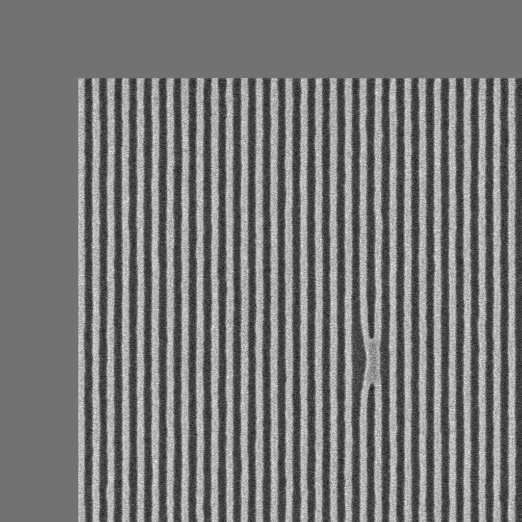
(d) Translation (+0.15)

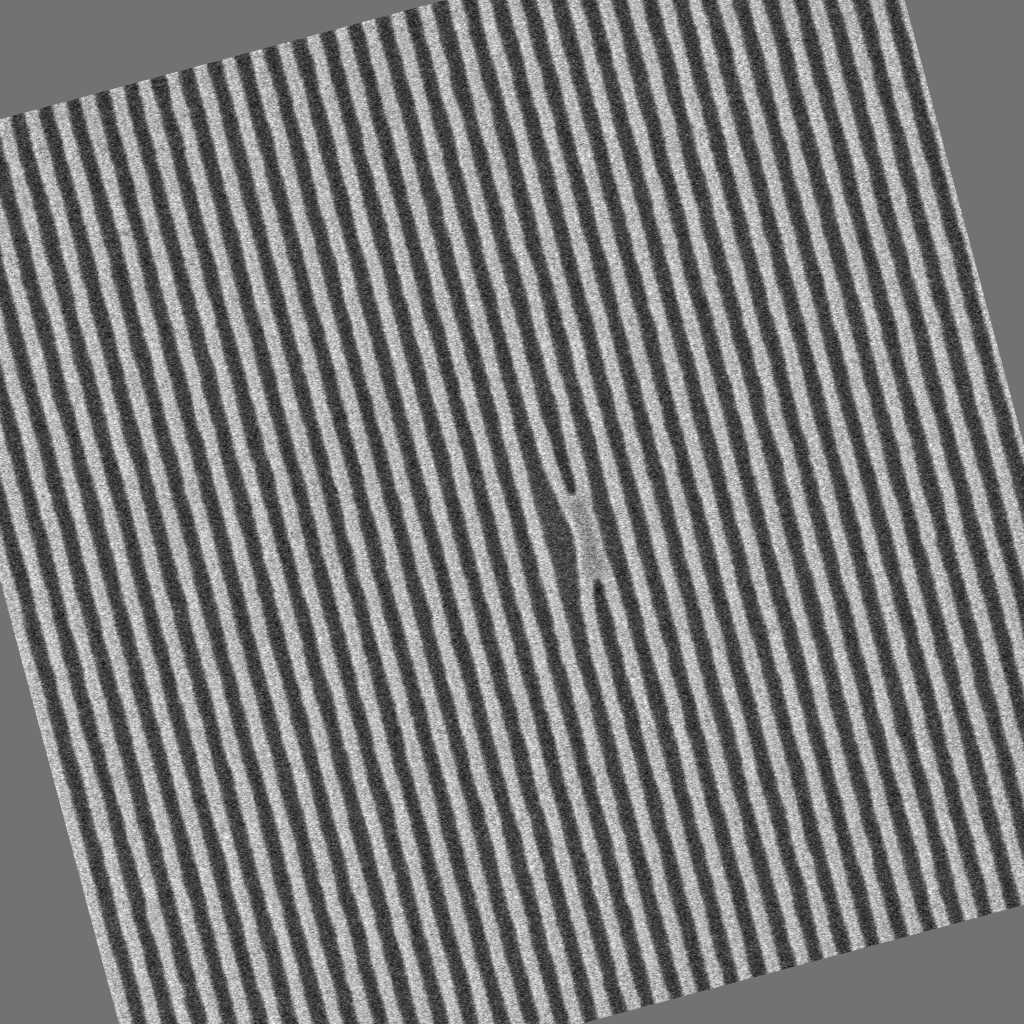
(e) Angle (15 degrees)

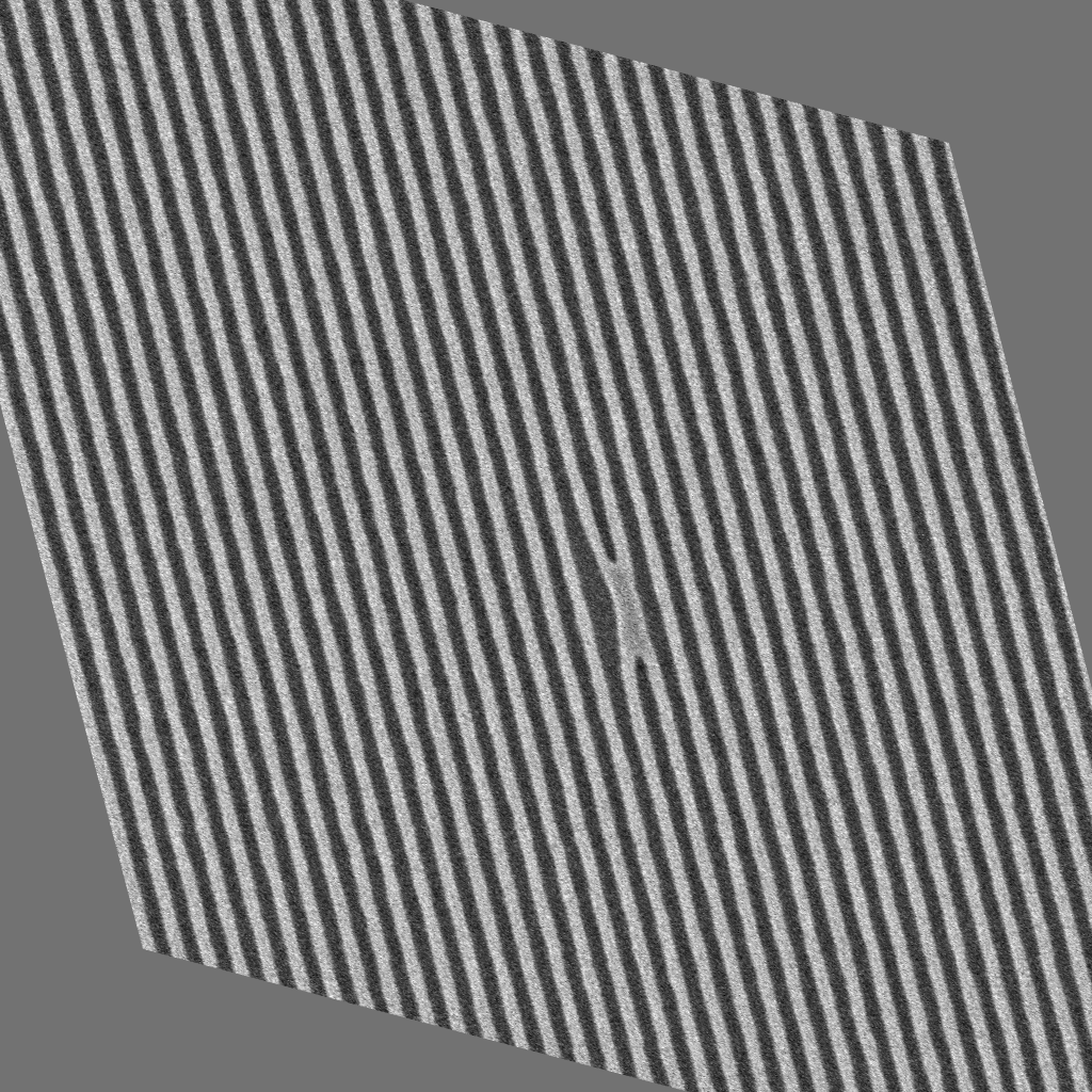
(f) Shear (+15 degrees)

(g) Hue (+0.5)

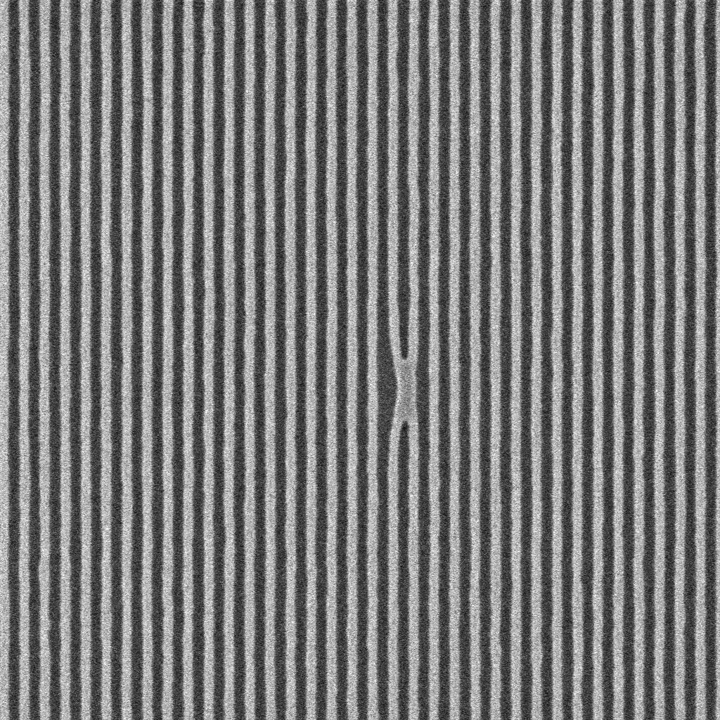
(h) Saturation (+0.5)

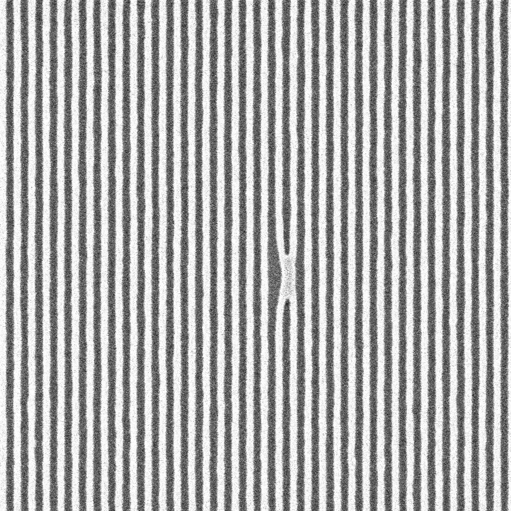
(i) Value (+0.5)

Figure 2: Data augmentation examples.

Detection models like YOLOv7 often predict multiple bounding boxes for the same instance. Therefore, combining these predicted boxes into a single final prediction is considered to be an important step for object detection. The most common prediction combination method of accomplishing is NMS. NMS groups predicted boxes for a class together when their intersection-over-unions are above a given threshold and removes all boxes except for the one with the highest confidence score. A more advanced method is WBF [10] which takes a weighted average of each box in a group to create the final prediction box. Figure 3, shows example predictions on a defect and how the NMS and WBF methods would combine the predictions. NMS is used by default for all models trained. We experiment with using WBF for the default model as well as ensemble models.

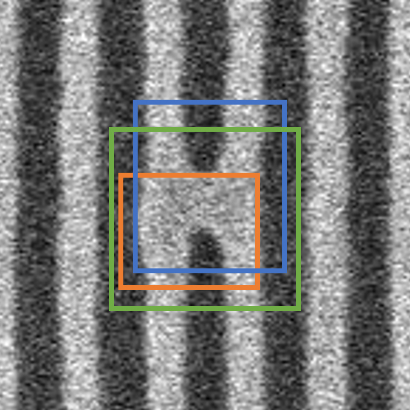
(a) Predictions before combination

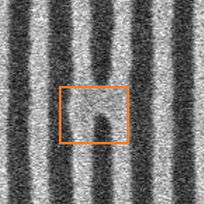
(b) NMS result

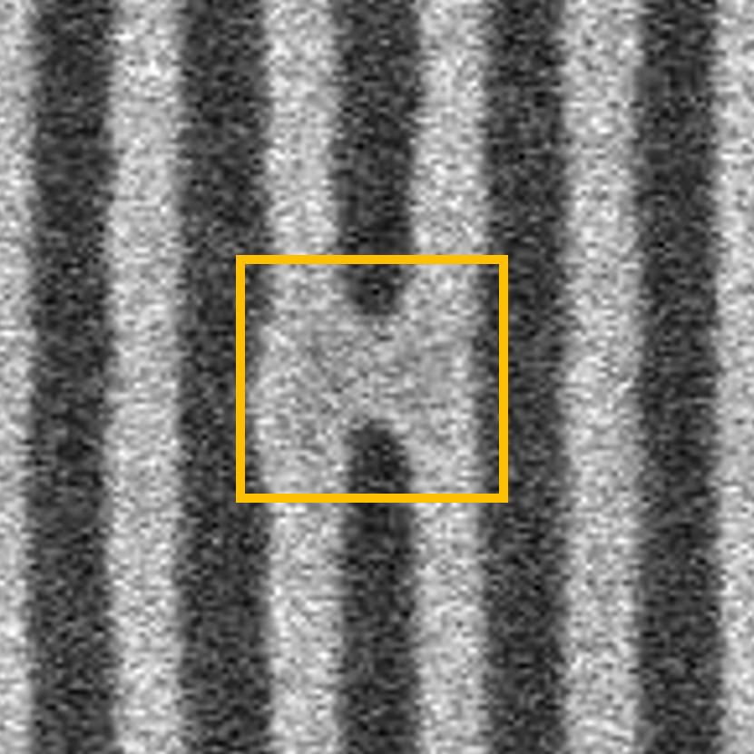
(c) WBF result

Figure 3: Example predictions for a bridge defect (3(a)) and corresponding final prediction examples after applying NMS (3(b)) and WBF (3(c)) combination algorithms. In this example, the orange prediction has the largest confidence score.

The best mean Average Precision (mAP) in the study by Dey et al. was achieved by an ensemble model consisting of three RetinaNet models with ResNet backbones of different sizes[1]. In addition to an ensemble model of YOLOv7 models of different sizes (Tiny, Base, and Base-X), we also ensembled models trained with different hyperparameters that achieve the best AP for different defect classes. Figure 4 depicts how ensemble models work on a conceptual level.

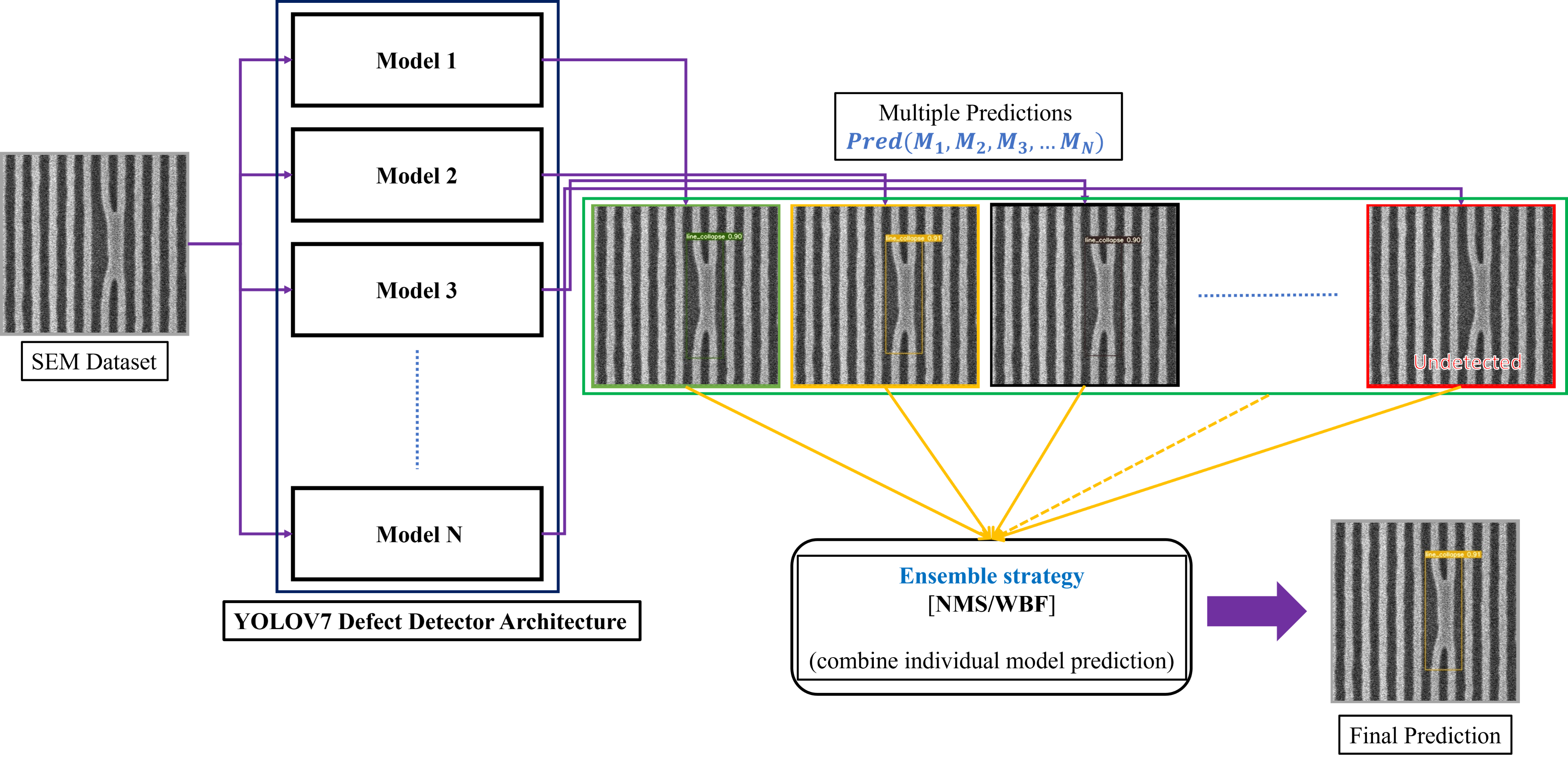
Figure 4: The ensemble framework generalized to N models. The final prediction of the ensemble model reflects the detection with the highest confidence score (NMS).

4 Experimental Setup

Code from the official YOLOv7 and WBF GitHub repositories were used to implement the experiments. All models were trained with a batch size of 2 for 200 epochs. At each epoch, evaluation was performed on the validation split. For each model, the trained checkpoint that achieved the best mAP at an IOU threshold of 0.5 was chosen for evaluation on the test split. All experiments were run on a Lambda Vector workstation with an NVIDIA GeForce RTX 3070 GPU.

5 Results & Discussion

The base YOLOv7 model with default hyperparameters achieves an mAP score of 0.790. This outperforms the best RetinaNet[11] models from Dey et al.[1] (0.787/0.775/0.788 for ResNet50/101/152 backbones[12], respectively). As will be shown in the rest of this section, the default YOLOv7, with hyperparameters optimized for natural image object detection, achieves a better mAP score than all but one of the models trained with different hyperparameters.

Table 3 shows the per-class AP and overall mAP on the test images for models with different “weights & learning” hyperparameter values. All models trained with a modified hyperparameter achieve lower mAPs than the default model. This shows that manually tuning hyperparameters for a certain dataset is difficult. Future work should instead employ hyperparameter optimization algorithms such as genetic algorithms, grid search, or bayesian optimization[13, 6]. Certain models do achieve better APs for the bridge and p-gap classes. Most notably, the Tiny model achieves a 36% better bridge AP than the default model.

Table 3: Per-class AP and overall mAP on the test images for all YOLOv7 base models with different “weights & learning” hyperparameter values. Bold values indicate that the default model’s value is the best or if the value is better than the default model’s results.

Hyperparameter	Value	AP (@0.5 IOU)
		microbridge	gap	bridge	line collapse	p-gap	All (mAP)
Default		0.873	0.967	0.602	1.000	0.508	0.790
Anchor threshold	9	0.806	0.950	0.639	1.000	0.529	0.785
	13	0.792	0.958	0.537	1.000	0.238	0.705
Anchors	9	0.726	0.948	0.587	1.000	0.167	0.686
	13	0.766	0.948	0.477	0.000	0.103	0.574
IOU threshold	0.1	0.737	0.950	0.590	1.000	0.150	0.685
	0.75	0.807	0.959	0.609	1.000	0.163	0.708
Object loss gain	0.25	0.754	0.949	0.581	1.000	0.274	0.712
	0.5	0.800	0.959	0.750	1.000	0.275	0.757
Class loss gain	0.1	0.737	0.950	0.590	1.000	0.150	0.685
	0.5	0.803	0.958	0.583	1.000	0.457	0.760
Box loss gain	0.1	0.762	0.959	0.562	1.000	0.106	0.678
	0.5	0.800	0.959	0.750	1.000	0.275	0.757
Focal-loss gamma	1.0	0.635	0.890	0.652	0.980	0.000	0.631
	1.5	0.581	0.851	0.505	1.000	0.000	0.587
Freeze layers	25	0.712	0.919	0.584	1.000	0.247	0.693
	50	0.745	0.949	0.579	1.000	0.139	0.682
Model size	Tiny	0.746	0.960	0.819	1.000	0.281	0.761
	Base-X	0.821	0.960	0.515	1.000	0.191	0.697

Table 4: Per-class AP and overall mean AP on the test images for all YOLOv7 base models with different “data augmentation” hyperparameter values. Bold values indicate that the default model’s value is the best or if the value is better than the default model’s results.

Hyperparameter	Value	AP (@0.5 IOU)
		microbridge	gap	bridge	line collapse	p-gap	All (mAP)
Default		0.873	0.967	0.602	1.000	0.508	0.790
Vertical Flipping	0.5	0.709	0.960	0.790	1.000	0.604	0.812
Horizontal Flipping	0.0	0.722	0.959	0.718	1.000	0.507	0.781
Mosaic[9]	0.0	0.647	0.952	0.581	1.000	0.030	0.642
	0.5	0.780	0.949	0.589	1.000	0.277	0.719
Scale	0.25	0.822	0.949	0.437	1.000	0.288	0.699
	0.75	0.758	0.939	0.634	1.000	0.133	0.693
Translation	0.0	0.784	0.968	0.540	1.000	0.107	0.680
	0.5	0.808	0.940	0.457	1.000	0.195	0.680
Angle	45	0.633	0.959	0.912	1.000	0.268	0.754
	90	0.597	0.899	0.745	1.000	0.055	0.659
Shear	15	0.779	0.967	0.548	1.000	0.277	0.714
	30	0.785	0.968	0.575	1.000	0.346	0.735
HSV	0.0	0.781	0.949	0.586	1.000	0.326	0.729
	1.0	0.677	0.949	0.584	1.000	0.197	0.681

Table 4 shows the AP results for models with different “data augmentation” hyperparameter values. We find that vertically flipping images randomly during training yields a 19% improvement in the AP for the most difficult defect class, probable gap, and a 3% improvement in the mean AP of all defect classes. This makes sense since a semiconductor SEM image flipped vertically shares the same characteristics as an image the model might encounter at inference time. Other hyperparameters don’t achieve a better mAP score than the default model. However, just like the “ weights & learning” hyperparameters, some other data augmentations hyperparameters do improve on AP for certain classes. Notably, tilting images randomly at an angle no greater than 45 degrees achieves the best bridge AP, 0.912, of all models tested.

Table 5 shows the AP results for different ensembles of models with either NMS or WBF prediction combination methods. The most impressive improvements come from ensembling models and applying WBF. All ensemble models achieve better per-class AP results for all classes and better mAP results than the default model alone. Applying WBF to the default model and to ensembles also improved mAP. Combining predictions from different models of different sizes using NMS and WBF improves mAP by 4% and 7%, respectively. The default, vertical flipping, and 45-degree angle models were chosen for the ensemble of models of different hyperparameter values that achieve best per-class performances. These models achieved the best microbridge, probable gap, and bridge results, respectively. This ensemble achieved the best mAP. Combining predictions from these models combined using WBF improved the mAP of the default model by 10% and the mAP of the size ensemble using WBF by 3%. The tradeoff here is reduced per-class APs for stand-out individual class results like for bridge defects where the AP of the model with 45-degree angle data augmentation is 7% better than the ensemble’s bridge AP.

Table 5: Per-class AP and overall mean AP on the test images for all YOLOv7 ensembles with either NMS or WBF prediction combination methods. Bold values indicate that the default model’s value is the best or if the value is better than the default model’s results. Blue values indicate the best value.

Models	Prediction	AP (@0.5 IOU)
	combination	microbridge	gap	bridge	line collapse	p-gap	mAP
Default	NMS	0.873	0.967	0.602	1.000	0.508	0.790
	WBF	0.709	0.960	0.790	1.000	0.604	0.812
Default, Tiny, Base-X	NMS	0.849	0.968	0.760	1.000	0.546	0.825
	WBF	0.852	0.968	0.823	1.000	0.565	0.842
Default, Vertical Flipping, Angle	NMS	0.877	0.969	0.809	1.000	0.634	0.858
	WBF	0.878	0.969	0.850	1.000	0.642	0.868

6 Conclusion

In this paper, we optimized the YOLOv7 model architecture for semiconductor defect detection by manually modifying hyperparameters and combining predictions from different models. Flipping images vertically during training was the only hyperparameter shown to improve mean Average Precision (mAP) compared to a model trained with default hyperparameters. However, modifying some other hyperparameters resulted in better AP scores for particular defect classes. Combining predictions from models trained with different hyperparameter values that achieved the best APs for different classes significantly improved mAP. Using the Weighted Box Fusion (WBF) method for combining predictions was shown to improve the results. Ultimately, the best per-class AP ensembling strategy with WBF achieves an mAP that is 10% better than using a single YOLOv7 model with default hyperparameters. Future work could improve on the results found in this study by using advanced hyperparameter optimization techniques.

References

- [1] Dey, B., Goswami, D., Halder, S., Khalil, K., Leray, P., and Bayoumi, M. A., “Deep learning-based defect classification and detection in SEM images,” in [Metrology, Inspection, and Process Control XXXVI ], Robinson, J. C. and Sendelbach, M. J., eds., SPIE (June 2022).
- [2] Imoto, K., Nakai, T., Ike, T., Haruki, K., and Sato, Y., “A cnn-based transfer learning method for defect classification in semiconductor manufacturing,” in [2018 International Symposium on Semiconductor Manufacturing (ISSM) ], 1–3 (2018).
- [3] Cheon, S., Lee, H., Kim, C. O., and Lee, S. H., “Convolutional neural network for wafer surface defect classification and the detection of unknown defect class,” IEEE Transactions on Semiconductor Manufacturing 32(2), 163–170 (2019).
- [4] Wang, Z., Yu, L., and Pu, L., “Defect simulation in SEM images using generative adversarial networks,” in [Metrology, Inspection, and Process Control for Semiconductor Manufacturing XXXV ], Adan, O. and Robinson, J. C., eds., 11611, 116110P, International Society for Optics and Photonics, SPIE (2021).
- [5] Dehaerne, E., Dey, B., and Halder, S., “A comparative study of deep-learning object detectors for semiconductor defect detection,” in [2022 29th IEEE International Conference on Electronics, Circuits and Systems (ICECS) ], 1–2 (2022).
- [6] Dey, B., Dehaerne, E., and Halder, S., “Towards improving challenging stochastic defect detection in SEM images based on improved YOLOv5,” in [Photomask Technology 2022 ], Kasprowicz, B. S., ed., 12293, 1229305, International Society for Optics and Photonics, SPIE (2022).
- [7] Wang, C.-Y., Bochkovskiy, A., and Liao, H.-Y. M., “YOLOv7: Trainable bag-of-freebies sets new state-of-the-art for real-time object detectors,” arXiv preprint arXiv:2207.02696 (2022).
- [8] Redmon, J., Divvala, S., Girshick, R., and Farhadi, A., “You only look once: Unified, real-time object detection,” (2015).
- [9] Bochkovskiy, A., Wang, C.-Y., and Liao, H.-Y. M., “Yolov4: Optimal speed and accuracy of object detection,” (2020).
- [10] Solovyev, R., Wang, W., and Gabruseva, T., “Weighted boxes fusion: Ensembling boxes from different object detection models,” Image and Vision Computing , 1–6 (2021).
- [11] Lin, T.-Y., Goyal, P., Girshick, R., He, K., and Dollár, P., “Focal loss for dense object detection,” in [2017 IEEE International Conference on Computer Vision (ICCV) ], 2999–3007 (2017).
- [12] He, K., Zhang, X., Ren, S., and Sun, J., “Deep residual learning for image recognition,” (2015).
- [13] Yang, L. and Shami, A., “On hyperparameter optimization of machine learning algorithms: Theory and practice,” Neurocomputing 415, 295–316 (2020).