newfloatplacementnewfloatnamenewfloatfileextnewfloatwithin

Partial differential equation-based inference of migration and proliferation mechanisms in cancer cell populations

Abstract

Targeting signaling pathways that drive cancer cell migration or proliferation is a common therapeutic approach. A popular experimental technique, the scratch assay, measures the migration and proliferation–driven cell monolayer formation. Scratch assay analyses do not differentiate between migration and proliferation effects and do not attempt to measure dynamic effects. To improve upon these methods, we combine high-throughput scratch assays, continuous video microscopy, and variational system identification (VSI) to infer partial differential equation (PDE) models of cell migration and proliferation. We capture the evolution of cell density fields over time using live cell microscopy and automated image processing. We employ VSI techniques to identify cell density dynamics modeled with first-order kinetics of advection-diffusion-reaction systems. We present a comparison of our methods to results obtained using traditional inference approaches on previously analyzed 1-dimensional scratch assay data. We demonstrate the application of this pipeline on high throughput 2-dimensional scratch assays and find that decreasing serum levels can decrease random cell migration by approximately $20\%$. Our integrated experimental and computational pipeline can be adapted for automatically quantifying the effect of biological perturbations on cell migration and proliferation in various cell lines.

Appendix A Introduction

Cell migration is a complex, multiscale phenomenon that integrates many different inputs and cell behaviors, including directed motion and random motion, that are differentially regulated by signaling kinases, cell density, and other factors^{1, 2}. Cell migration helps maintain or form tissues or monolayers both in vivo and in vitro^{3, 4}; cell division also contributes to the development or maintenance of these multicellular structures. Further, cell migration is associated with cancer metastasis, and thus is commonly studied in the context of oncogenic mutations or cancer treatments. Because cell migration integrates so many different parts of the cell, inferring relationships between perturbations and migratory outputs is challenging. Drugs could affect one or more different drivers of cell migration, potentially in different ways, with unpredictable overall effects on cell migration. Cell migration is commonly measured using scratch assays, where a monolayer of cells is scratched to physically remove cells in a localized region⁵. Subsequently, migration into the newly emptied space is measured over time. These measurements are commonplace in biological research, and have for instance been used to identify novel inhibitors of cell migration or genes responsible for regulating migration^{6, 7}. However, typically the complexity of cell migration is reduced to a single number, which represents the amount of space filled in a given time or the distance traveled by the leading edge of cells. This singular number obscures the behavioral changes that cause changes in migration and could for instance fail to identify differences between drugs which inhibit migration to the same degree, but through the modulation of either directed migration or cell proliferation. Thus, the utility of scratch assays could be improved by identifying relationships between perturbations and specific biological effects.

Computational and mathematical modeling of cell migration has been used to extract granular, quantitative information from scratch assays. First-principles modeling has established a variety of partial differential equation (PDE) models that accurately represent the behavior of scratch assays in a variety of conditions^{8, 9}. These models commonly include reaction terms, which represent cell growth or death, and diffusion terms, which represent random cell motion, with various functional forms. For example, some models use a reaction equation corresponding to cells growing with a constant growth rate, affected by a maximum carrying capacity. Other terms, including advection (directed cell migration), could also be included in cases such as chemotaxis or migration to regions of lower cell density where cells have a directional movement stimulus. By estimating parameters for these models, past work has helped identify quantitative effects of biological perturbations in scratch assays^{8, 10, 11}. However, any individual model may not be flexible enough to account for behaviors observed in novel experimental conditions.

Recent work has also established the use of physics-informed neural networks to model cell migration in scratch assays¹⁰. In this approach, a neural network is trained to predict the progression of cell concentrations over time. During training, the neural network optimizes a loss function which penalizes both inaccurate predictions and deviations from a pre-defined reaction-diffusion model. In this way, the neural network learns density-dependent growth and diffusion terms which best fit the data. However, neural networks can learn arbitrary relationships to make predictions, and there is no guarantee that the growth or diffusivities learned are physically realizable.

Another method for learning governing PDEs from experimental data and known physical constraints is variational system identification (VSI)^{12, 13, 14}. VSI enables modelers to identify a family of potential basis operators (e.g, polynomials, trigonometric functions, exponential functions, and differential terms) which make up the PDE. VSI then identifies parsimonious models incorporating subsets of basis operators by iteratively dropping bases. A key advantage of VSI is that it does not require forward evaluations of the model while dropping bases, which substantially reduces computational cost. VSI has been applied to identify governing equations for the evolution of materials as well as the spatiotemporal spread of COVID-19^{12, 13, 14}. After identifying a sparse basis for the governing PDEs for a given set of data, the sparse model can be fine-tuned using adjoint optimization and the learned model can be validated against experimental data. Finally, the model bases and parameters can be compared among models learned from different datasets in different conditions in order to extract quantitative insights from data.

We hypothesized that VSI could be used to quickly and quantitatively model wound healing data, providing quantitative comparisons between different conditions. To test this hypothesis, we first applied VSI to previously published wound healing data. VSI was able to rapidly identify an accurate model describing the evolution of cell concentration over time for a variety of initial seeding densities. VSI identified reaction and diffusion terms underlying the observed behavior, consistent with previous results. We next applied VSI to our own data. We performed scratch assays on MDA-MB-231 breast cancer cells under a variety of conditions and used automated image processing to extract cell concentration fields over time. We found that VSI could successfully model 2-D scratch assays, and we further quantified the effect of serum concentration on cell diffusion and reaction. VSI represents a useful modeling approach to rapidly identify plausible models for cell migration and quantify model effects in different experimental conditions.

Appendix B Methods

Cell Culture

We cultured MDA-MB-231 breast cancer cells in Dulbecco’s Modified Eagle Medium (DMEM) with $10\%$ fetal bovine serum (FBS). We passaged cells at a 1 to 10 ratio when they were approximately $90\%$ confluent. For imaging experiments, we cultured cells in imaging media, consisting of fluorobrite phenol red-free medium supplemented variable FBS (depending on desired experimental conditions), 1X penicillin/streptomycin, 1X GlutaMAX, and 1X sodium pyruvate. Sodium pyruvate was added as an antioxidant to reduce imaging-induced stress.

Stable Cell Line Generation

We engineered the MDA-MB-231 cells used in this work to stably express 3 fluorescent proteins: kinase translocation reporters (KTRs) for kinases Akt (mAquamarine) and ERK (mCitrine), and a stable histone-2B (H2B) nuclear marker (mCherry), as described previously^{15, 16}. MDA-MB-231 cells also expressed a puromycin selection marker. The plasmid containing H2B-mCherry, AktKTR-mAqua, ERKKTR-mCitrine, and puromycin selection is referred to as pHAEP. Expression was achieved using a PiggyBac transposon vector. Cells were then selected using puromycin.

Scratch Assay and continuous fluorescence imaging

For scratch assay experiments, we seeded 50,000 MDA-MB-231 pHAEP cells in 1 ml imaging media in a 24-well glass-bottom imaging plate. We grew cells to full confluency (approximately 36 hours) before starting the scratch assay. For the scratch assay, we manually scratched each cell monolayer using a p200 pipette tip. Immediately after scratching, we washed the cells with 1 ml warm phosphate buffered saline (PBS) and then added 1 ml of warm imaging media containing experimental treatments. We imaged cells using an EVOS M7000 fluorescent microscope with on-stage incubator. After scratching each well, we placed the well plate into the prepared EVOS incubator. The incubator was maintained at 37°C, $5\%$ CO2, and $>80\%$ humidity. For continuous imaging, we captured continuous fields centered on the scratch near the center of each well. We imaged three channels with 10x magnification, corresponding to mCherry, mAqua, and mCitrine fluorescent proteins. We acquired images every 20 minutes over 24-48 hours in all wells in the well plate. We imaged one region of the scratch per well.

Automated image processing

We processed fluorescent images as described previously¹⁷. Image processing was performed using MATLAB. Briefly, we first threshold the nuclear images using an adaptive thresholding method. After identifying nuclear pixels, we extract the centroid pixel of each distinct nuclear object. To quantify KTR activity, we next identify cytoplasmic pixels by expanding the nuclear mask by 10 pixels. We calculate cytoplasmic and nuclear intensities using the average intensity in each KTR channel in the cytoplasmic ring and nucleus, respectively. In contrast to previous work, we do not track cells between frames. The output of image processing for one well is a set of quantified cell data including nuclear location and KTR quantification at each time point. We apply this to each well in the dataset. After automated image processing, we extract cell density fields c(x, y, t) from each well in the experiment. To do so, we apply spatial binning to the cell positions. Bin sizes between 50 and 100 microns were used. We smooth it in both space and time. We applied a rolling mean with a window of 3 to spatial data and a window of 11 to temporal data. Smoothing the data reduces numerical instabilities in the calculation of derivatives. We calculate spatial and temporal derivatives at this step.

Wound healing quantification

We quantified wound closure by identifying the distance between wound edges at the first (dstart) and last (dend) timepoints in the experiment. We estimated the position of the front of each wound as a line and calculated the distance in the x direction (perpendicular to the wound) between each wound front. Then, we calculated wound closure as:

$$\text{Wound closure}=\frac{d_{\text{start}}-d_{\text{end}}}{d_{\text{start}}}$$ (1)

Appendix C Continuum-scale data-driven modeling for cell migration

The density of cells is defined as a spatiotemporal field, $C(\mbox{\boldmath$x$},t)$ with $(\mbox{\boldmath$x$},t)\in\Omega\times[0,T]$ where $\Omega$ and $[0,T]$ are the spatial domain and time period of interest. The evolution of this field is described using the following first-order kinetics:

$$\frac{\partial C}{\partial t}=L[C;\boldsymbol{\theta}]$$ (2)

where, $L$ is a differential operator parameterized by $\boldsymbol{\theta}$. Numerical solutions of the PDEs are typically estimated as a finite dimensional expansion of $C$ (in appropriate functional spaces) that drives a residual to vanish:

$$R(C^{\ast};\boldsymbol{\theta})=0;\qquad R=\frac{\partial C}{\partial t}-L[C;\boldsymbol{\theta}]$$ (3)

where $C^{\ast}$ is the approximate solution in the functional space, $\mathcal{F}$ for fixed choice of parameters, $\boldsymbol{\theta}$. The residual, $R$ can be thought of as an error in the sense that it quantifies the extent to which the PDE fails to be satisfied for a given function, $C^{\ast}$. System identification methods, on the other hand, follow an optimization approach where the parameters are estimated based on the observed data. This minimization problem can be posed as follows:

$$\boldsymbol{\theta}^{*}=\operatorname*{arg\,min}_{\boldsymbol{\theta}\in\boldsymbol{\Theta}}\left|\left|\mbox{\boldmath$R$}(\boldsymbol{\theta}|C^{d})\right|\right|$$ (4)

where $\boldsymbol{\theta}^{*}$ denotes the optimal parameters chosen from the set of admissible parameters, $\boldsymbol{\Theta}$. The observed (data) density field from experiments is denoted as $C^{d}$. It should be noted that this method doesn’t require solving a PDE, making it amenable to estimating parameters even in nonlinear PDEs. This approach reduces the problem of parameter estimation to a regression problem that is fairly inexpensive to solve computationally. This allows us to start with a large possible basis of terms for $L$ and subsequently drop the insignificant ones using approaches like regularization and stepwise regression. Here we have intentionally omitted certain details like the choice of norm, $||.||$ and functional space, $\mathcal{F}$, in favor of presenting the basic idea of system identification. In finite element methods for solving PDEs, the residual of the problem is formulated using the weak form of the PDE, instead of the strong form as in (3). We will adopt the residual written in terms of the weak form in our PDE inference, and thus refer to it as Variational System, Identification^{12, 13, 14}. It is described next.

Variational formulation for Advection Diffusion Reaction system

The advection-diffusion-reaction equation is employed to represent transport of cell density, and is encoded in the operator, $L$. Mechanistically, the advection represents the directed motion of the cells, diffusion represents their random motion and reaction models cell death or proliferation. The advection-diffusion-reaction equation is given as follows:

$$\frac{\partial C}{\partial t}=\nabla\cdot\left(D\nabla C\right)-\nabla\cdot(Cv_{f}\mbox{\boldmath$v$}_{\text{unit}})+r$$ (5)

where $D$ is diffusivity, $v_{f}$ is advective speed, $\mbox{\boldmath$v$}_{unit}$ is a unit vector perpendicular to wound, and $r$ is the cell reaction rate. Here, we consider functions of cell density, $D(C)$, $v_{f}(C)$, and $r(C)$. There exist models that have considered density-dependent effects on migration, for instance due to cells interacting with each other, and on cell proliferation, for instance, due to inhibition at high cell density.. ^{8, 18} We solve the weak form of Eq. 5:

$$\int_{\Omega}\frac{\partial C}{\partial t}wd\Omega =\int_{\Omega}\left(-D\nabla w\cdot\nabla C+Cv_{f}\mbox{\boldmath$v$}_{\text{unit}}\cdot\nabla w+r\right)wd\Omega+\int_{\partial\Omega}w\left(D\nabla C-Cv_{f}\mbox{\boldmath$v$}_{\text{unit}}\right).\mbox{\boldmath$n$}ds$$ (6)

where $w$ is the weighting function commonly used in variational calculus. The weak form leads to the following residual:

$$R =\int_{\Omega}\left(\frac{\partial C}{\partial t}Nd\Omega+D\nabla N\cdot\nabla C-Cv_{f}\mbox{\boldmath$v$}_{\text{unit}}\cdot\nabla N-rN\right)d\Omega-\int_{\partial\Omega}N\left(D\nabla C-Cv_{f}\mbox{\boldmath$v$}_{\text{unit}}\right).\mbox{\boldmath$n$}ds$$ (7)

where $N$ is the vector of finite elements and $n$ is the unit normal vector for the boundary $\partial\Omega$. We can rewrite this equation as a matrix-vector problem with the following form, with $A_{e}$ representing the finite element assembly operator.

The discretization-based numerical solition of this PDE is known to have spatial instabilities for highly advective flows. These instabilities are mitigated by adopting streamline-upwind/Petrov-Galerkin (SUPG) stabilization. This is achieved by augmenting the residual as follows:

$$\widetilde{R}=R+\tau h\int_{\Omega}\left(\frac{dC}{dt}-\nabla\cdot\left(D\nabla C\right)+\nabla\cdot\left(C\mbox{\boldmath$v$}\right)-f\right)\left(\mbox{\boldmath$v$}\cdot\nabla w\right)d\Omega$$ (8)

This system of equation is solved using the Newton-Raphson method.

VSI for the Advection Diffusion Reaction system

We start with the following ansatz for the $D$, $v_{f}$ and $r$ parameters:

$$D =\boldsymbol{\theta}_{(0-2)}\cdot[1,C,C^{2}]$$ (9)

$$v_{f} =\boldsymbol{\theta}_{(3-5)}\cdot[1,C,C^{2}]$$ (10)

$$r =\boldsymbol{\theta}_{(6-7)}\cdot[C,C^{2}]$$ (11)

Note that the constant reaction term was omitted, since it could imply that cells either grow ($r>0$) or die ($r<0$) in a region with zero cell density.

$$\mbox{\boldmath$R$}(D,v_{f},r) =\mbox{\boldmath$y$}-\boldsymbol{\Xi}\cdot\boldsymbol{\theta}$$ (12)

$$y =-\mbox{\boldmath$A$}_{e}\left[\int_{\Omega_{e}}\frac{\partial C}{\partial t}\mbox{\boldmath$N$}d\Omega\right]$$ (13)

$$\boldsymbol{\Xi} \equiv\left[\boldsymbol{\Xi}_{0},\cdots,\boldsymbol{\Xi}_{7}\right].\$$ (14)

Now, $R$ is the residual vector, indexed and $y$ is a vector of time derivatives. $\boldsymbol{\Xi}$ is a matrix of spatial derivatives calculated at each time and point in the spatial domain. $\boldsymbol{\Xi}$ will be a matrix with $(N_{\text{points}}*(N_{\text{times}}-1))$ rows and $N_{\text{basis}}$ columns. $\boldsymbol{\Xi}$ is evaluated as:

$$\boldsymbol{\Xi}_{0,1,2} =\mbox{\boldmath$A$}_{e}\left[\int_{\Omega_{e}}\left[1,C,C^{2}\right]\nabla\mbox{\boldmath$N$}\cdot\nabla Cd\Omega-\int_{\partial\Omega_{e}}\left[1,C,C^{2}\right]\mbox{\boldmath$N$}\nabla C\cdot\mbox{\boldmath$n$}ds\right]$$ (15)

$$\boldsymbol{\Xi}_{3,4,5} =\mbox{\boldmath$A$}_{e}\left[-\int_{\Omega_{e}}\left[1,C,C^{2}\right]Cv_{f}\mbox{\boldmath$v$}_{\text{unit}}\cdot\nabla\mbox{\boldmath$N$}d\Omega+\int_{\partial\Omega_{e}}\left[1,C,C^{2}\right]NCv_{f}\mbox{\boldmath$v$}_{\text{unit}}\cdot\mbox{\boldmath$n$}ds\right]$$ (16)

$$\boldsymbol{\Xi}_{6,7} =\mbox{\boldmath$A$}_{e}\left[\int_{\Omega_{e}}\left[C,C^{2}\right]Nd\Omega\right]$$ (17)

The vector $\boldsymbol{R}$ holds the coefficients corresponding to the bases selected. $R$ and $y$ will both be column vectors with the number of rows equal to $(N_{\text{points}}*(N_{\text{times}}-1))$, since we can calculate time derivatives at each spatial point at every time except the first. The column vector $\boldsymbol{\theta}$ has $N_{\text{basis}}$ rows. We finally state the minimization problem solved by VSI to find the optimal bases:

$$\boldsymbol{\theta}^{*}=\operatorname*{arg\,min}_{\theta}||\mbox{\boldmath$R$}(\boldsymbol{C^{\text{d}};\theta})||_{2}^{2}$$ (18)

Stepwise regression for identification of parsimonious models

In favor of parsimony of the model, which can be quantified as the sparsity of bases terms, we intent to estimate the most significant terms in the prescribed ansatz for the parameters and drop all the insignificant ones. We perform stepwise regression to determine these significant terms^{12, 13, 14}. In this approach, we iteratively identify a term, that when eliminated from the basis, causes minimal change in the loss of the reduced optimization problem from Eq. 18.

$$\text{Loss}_{\text{VSI}}=||\boldsymbol{\Xi}\cdot\boldsymbol{\theta}-\boldsymbol{y}||_{2}^{2}$$ (19)

To avoid dropping more than the necessary terms, we perform the statistical F-test that signifies the relative change in loss with respect to change in number of terms. Therefore, we use a threshold for the F-value as a stopping criterion for stepwise regression. More details on this approach are provided in the previous works mentioned above. It should be noted that we do not allow elimination of the term with constant diffusivity, since a constant positive diffusivity confers spatial stability on admissible solutions.

PDE Constrained Optimization for model refinement

After using VSI to identify a parsimonious model that fits the data, adjoint-based PDE constrained optimization is applied to improve the fit. The procedure minimizes the following loss

$$\text{Loss}_{\text{Adj}}=||C(t)-C^{\text{d}}(t)||_{L_{2}(\Omega\times[0,T])}^{2}$$ (20)

Adjoint optimization requires running the forward model, which can be computationally expensive and require exploring regions of parameter space which are numerically unstable, making it unsuitable for large models. However, it can be applied to simpler models after VSI has identified a parsimonious model. To apply adjoint optimization, we start from the inferred VSI parameters. We solve the forward model based on experimentally observed initial conditions, generating a predicted cell density field and an associated loss. We use BFGS optimization to further minimize the loss. Adjoint optimization generates a new set of basis values which should fit the data better than the VSI-inferred model.

Appendix D Result

VSI learns dynamics of 1-D wound healing data

We first tested VSI on a previously reported scratch assay dataset. The dataset, collected by Jin et al.,⁴ consists of scratch assays performed on PC-3 prostate cancer cells with varying initial confluence prior to the scratch. Confluency was varied by varying the initial cell seeding density from 10,000 to 20,000 initial cells seeded. Cell density along the axis perpendicular to the scratch was measured in triplicate and averaged across replicates. Finally, 2-D cell density was averaged along the dimension perpendicular to the scratch, yielding one 1-D concentration field $C(x,t)$ for each initial density. To infer systems of governing equations, we first preprocessed and smoothed the data. The smoothed cell density profiles for initial seeding of 20,000 and 12,000 cells over time are shown in Fig. 1(A), and the rest are included in the appendix (see Fig. A.5). The scratch, which is approximately $800\mu m$, is clear in the initial density profiles. For initial seeding densities 14000 and higher, the center of the scratch (around $x=900\mu m$) is occupied by cells after 48 hours. Furthermore, there is an increase in cell density at the scratch edge (near $x=0\mu m\text{ or }1800\mu m$) over time for all initial seeding densities, indicating that the cells continue growing during the experiment.

As a proof of concept, we applied VSI to each of the 6 scratch assay data sets. We preprocessed the data generated bases for diffusivity, rate of advection, and reaction rate corresponding to polynomial functions of concentration up to order 2 (Fig. 1(C)).

Figure 1: VSI applied to previously analyzed 2D data A) Raw data for two scratch assay datasets analyzed here. Data was collected by Jin et al.⁴ and replotted. B) Basis selection corresponds to diffusion, advection, and reaction terms. C) VSI loss calculated as the mean squared error between the calculated time derivatives and predicted derivatives from each VSI step.D) The model fit to initial seeding of 20,000 cells contains 3 terms, corresponding to constant diffusivity (independent of concentration), diffusivity with quadratic dependence on concentration, and linear reactivity. E) Comparison between model fits (dashed lines) and smoothed experimental wound healing data (solid lines) over time for the Adjoint-optimized model fit to data from initial seeding of 20,000 cells.

We next use VSI to identify how many terms are necessary to fit the data. Fig. 1(D) shows that for all initial seeding densities, the loss (mean squared error between calculated and predicted time derivatives) does not decrease after more than 3 terms are included in the model. Thus, we infer that a smaller, three-term model could be used to fit the data. For all models, the three-term model excluded advection terms. We next performed adjoint optimization on the 3-term model for each initial seeding density. The adjoint optimized model for initial seeding density of 20,000 included linear and quadratic dependence of diffusivity on concentration and reaction that is linear with respect to concentration. After obtaining an optimized adjoint model, we used the identified coefficients to run a forward model from the initial conditions of the dataset seeded with 20,000 cells. The model predictions and experimental observations are shown in (Fig. 1(E)). The adjoint solution qualitatively fits the observed dynamics, and at later times fits quantitatively.

We compared the quantitative values we derived for diffusivity for each initial seeding density with previously derived reaction-diffusion models that assumed constant diffusivity and growth affected by a carrying capacity (Tab. 1).⁸ We use the constant diffusivity inferred, since for all systems the concentration dependence of diffusivity was weak. Our results substantially differ for all initial seeding densities except an initial density of 20,000 cells. However, the analysis by Jin et. al reveals that their model fits are very insensitive to exact diffusivity values. Furthermore, past applications of VSI and adjoint optimization have shown that inference of diffusivity is challenging. We compared the forward model predictions for cell concentration over time using our inferred parameters and the fit parameters from Jin et. al. We found that for 5 of the 6 initial seeding densities, our models have lower root mean squared error (RMSE), indicating better fits to experimental data, and the $6^{\text{th}}$ dataset is competitive (Fig. 2). These results suggest that our VSI-adjoint modeling approach can be used to infer models for cell migration dynamics that are competitive with more traditional methods.

	Diffusivity $(\mu m^{2}/hr)$
Initial Seeding density	Reaction Diffusion model 8	VSI+Adjoint
10,000	310	4.78
12,000	250	11.0
14,000	720	12.1
16,000	570	13.1
18,000	760	13.4
20,000	1030	697

Table 1: Comparison of diffusivity values learned from previous work⁸ and our VSI and adjoint method (constant with respect to concentration).

Figure 2: Root mean squared error (RMSE) calculated between experimental data and reaction-diffusion models from Jin et. al (blue) or adjoint optimization of a VSI model (red) for each initial seeding density.

VSI quantifies the effect of different conditions on migration dynamics in high-throughput, 2-dimensional scratch assays

After demonstrating that VSI could be used to learn parsimonious reaction-diffusion models for cell migration data in the literature, we used system identification on our cell density data gathered from high-throughput fluorescent microscopy experiments. We performed scratch assays using MDA-MB-231 breast cancer cells stably expressing a fluorescent nuclear marker and kinase translocation reporters for the Akt and ERK pathways. We used these cells to perform scratch assays in 24-well plates and tracked scratch closure over time using live-cell fluorescence microscopy.

Figure 3: Fractional wound closure calculated for two different conditions. For $10\%$ serum, $N=2$ wells, and for $3\%$ serum, $N=3$ wells

We first used this assay to compare how fetal bovine serum (FBS) affects cell migration. FBS is a cocktail of growth factors and compounds that can drive cell migration, and therefore lower FBS concentration should slow wound healing due to slower cell division and migration. We captured wound-closure dynamics for cells cultured in $10\%$ FBS and $3\%$ FBS over 24 hours. We observed that $3\%$ serum decreased the average wound closure from $38\%$ to $29\%$, although the difference was not statistically significant (Fig. 3).

We next applied our VSI pipeline to infer models for the observed wound closure dynamics. We used the same set of basis functions, including constant, linear, and quadratic terms for diffusion and advection and linear and quadratic terms for reaction. We fit a model to the replicate conditions simultaneously, generating a single model for each condition. Finally, we ran learned the adjoint model for both conditions starting from experimental initial conditions (Fig. 4(A)). We again observed that the VSI loss function is essentially constant for models including diffusive and reaction terms, and only starts to increase for models that lack reaction terms (Fig. 4(A)). Based on the VSI results, we utilized a 3 term model. For both $10\%$ and $3\%$ serum, these terms corresponded to constant diffusivity and linear and quadratic reaction. We compared the terms identified for each model, and find that according to our adjoint model, diffusivity decreases by approximately $20\%$, from $202\mu m^{2}/hr$ to $166\mu m^{2}/hr$, in $3\%$ serum compared to $10\%$ serum (Fig. 4(C)). VSI infers a non-linear relationship between reaction (cell proliferation) rate and cell density, suggesting that the reaction/proliferation rate is positive at low concentrations and then becomes negative above a critical concentration (Fig. 4(D)). The models inferred for $10\%$ and $3\%$ serum conditions suggest that decreasing serum causes a decrease in random cell migration but does not substantially affect cell proliferation.

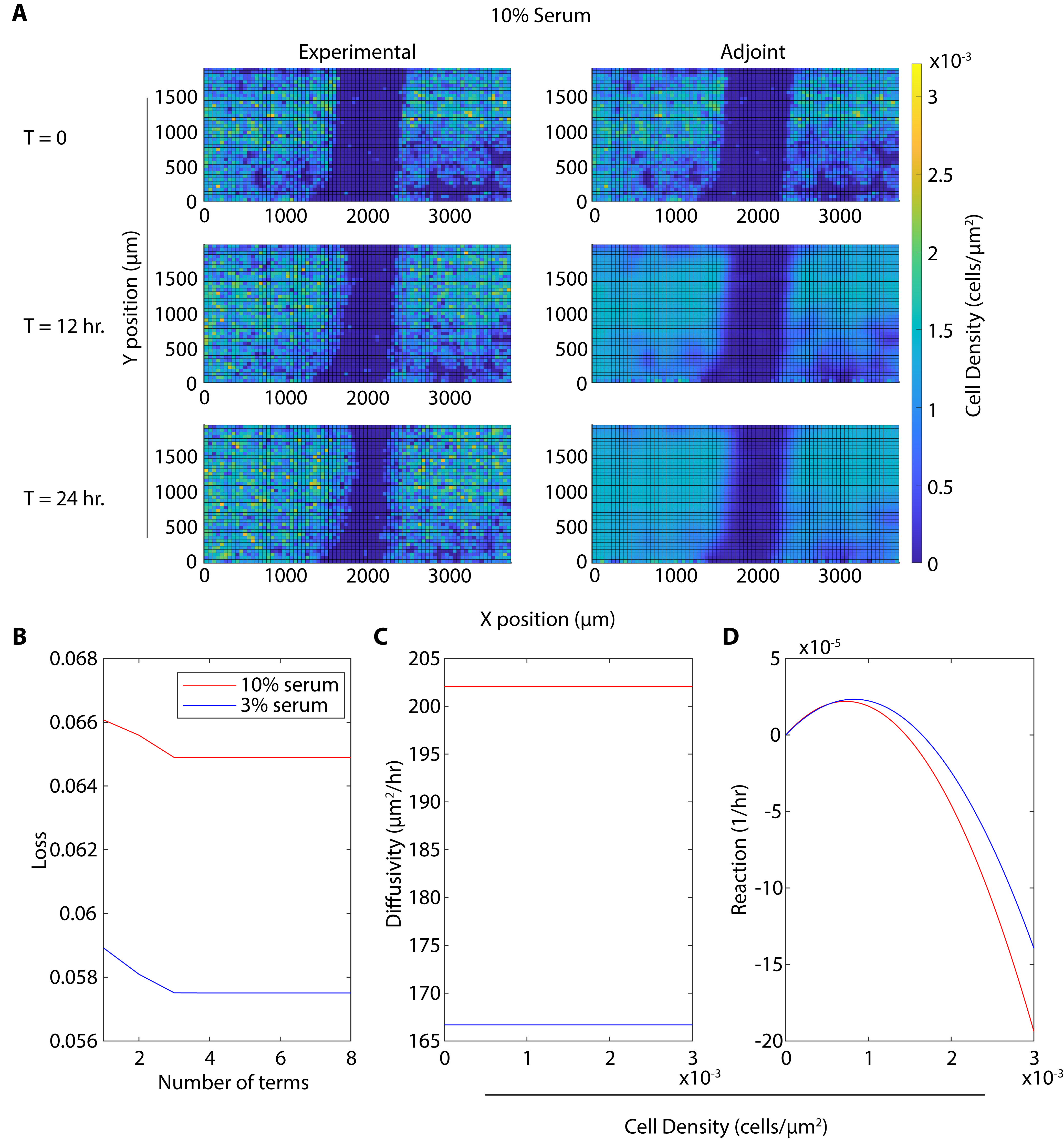
Figure 4: A) Comparison of experimental data and adjoint model predictions from same initial conditions. B) VSI loss as a function of VSI bases selected. C-D) Adjoint optimized diffusivity (C) and reaction (cell proliferation) (D) terms as functions of concentration. Diffusivity is constant, while reaction/proliferation is a combination of linear and quadratic bases. The $x$-axis ranegs were chosen to represent the concentrations present in the experimental data.

Appendix E Discussion

Here, we demonstrate that VSI can infer parsimonious, quantitative and physics-based models for collective cell migration. In a 1D setting, we infer models with accuracies that are competitive to other methods. Notably, there are substantial differences between our inferred diffusivity and previous work. We also apply our method to 2D wound healing experiments. Relative to the 1D data, our 2D wound healing experiments were sampled more frequently (every 20 minutes compared to every 12 hours) with similar spatial resolution. In this setting, we estimate diffusivity values for breast cancer cells between 165 and 205 $\mu m^{2}/hr$. Previous computational analyses of cell migration have identified a wide range of diffusivity values, from approximately 50 to 3000 $\mu m^{2}/hr$^{9, 19, 20}. Thus, our estimates of diffusivity in the 1D and 2D settings are consistent with prior literature.

There are several advantages and disadvantages to PDE inference by VSI compared to other approaches such as traditional model inference or physically informed neural networks (PINNs). Traditionally, building models of cell migration has utilized iterative cycles of model conceptualization, based on known cell biology, that include increasingly complex models for cell division or diffusion. These models are informative and have made substantial progress towards a general theory of collective cell migration. However, model development can require a substantial amount of expertise or trial and error. Furthermore, this approach does not scale well if new sources of data are acquired, which could cause exponential increases in the number of potential model terms based on the interaction of a new data source with all other types of data previously considered in the model. For example, data about cell state (e.g. signaling activity, cell-cycle status, metabolic activity) gathered from fluorescent reporters or cell morphology could require updating a model to consider diffusivity as a function of both cell state and local cell density^{3, 21, 22, 23}. Hence, we envision that VSI can improve traditional modeling in at least two ways. First, it could serve as a hypothesis testing tool. Faced with a large set of potential models incorporating various sources of data, modelers could use VSI to identify data sources (in the form of bases) that are relatively uninformative for the desired modeling task, enabling them to rapidly focus on the bases, and therefore data sources, that are most helpful. Then, they could develop mechanistic models that focus on those data sources. Second, VSI could enable rapid prototyping of models, where data is quickly interpreted using identified models and used to generate new experimental conditions. Traditional modeling can be time consuming, and a more rapid, semi-automated modeling approach such as VSI could lead to more tightly coupled model-driven experimentation.

Other modeling approaches have used neural networks to perform data-driven inference on reaction and diffusion equations governing cell migration. In VSI, the equations learned are confined to the bases used, while neural networks can learn arbitrary relationships for equation parameters to best fit the data. Lagergren et al. demonstrated the power of this approach on the Jin et al. dataset (also analyzed in ⁸), when they inferred density-dependent reaction-diffusion equations for cell migration¹⁰. They identified non-linear functions of concentration for diffusivity and reaction terms, and found that these functions vary with initial seeding concentration, consistent with our findings. There is one noteworthy difference between neural network-based approaches and VSI. In the case of cell migration, the neural networks can learn arbitrary relationships between cell density and diffusivity or reaction. Thus, there is no guarantee that the neural network learns physically realizable diffusivity or reaction relationships. VSI, on the other hand, enables the modeler to explore various bases and consider how each might be captured by a physical relationship. PINNs can discover relationships that maximize the fit to data, while VSI sacrifices fitting to data because it is constrained to selected bases which the modeler can ensure are physically meaningful.

We envision two key applications of VSI furthering our understanding of biology. First, VSI can be used to quantify the effects of drugs in high-throughput screens. Scratch assays have been miniaturized and mechanized, making them compatible with high-throughput screening^{24, 25}. Thus, VSI could be combined with high-throughput drug screens and the specific effects of drugs on cell migration and division could be determined. Second, VSI could be used to rapidly infer models based on new streams of data gathered from scratch assays. Cell morphology²¹ and fluorescent reporters²³ have been used to measure or infer cell states in migrating cells. Thus, VSI could be used to capture diffusivity or reaction terms as functions of not only cell density but also local measures of cell state.

Appendix F Conclusion

In summary, we demonstrate that variational system identification can be used to rapidly infer partial differential equation models that model collective cell migration in a wound healing assay. We benchmark this method by comparing inferred models with previous reaction-diffusion models applied to 1-D wound healing data, finding that our models are comparable or slightly superior in accuracy to the previously published, traditionally derived models. We next capture cell migration in 2-D wound healing assays using video microscopy, measuring the effect of serum on cell migration as a test case. We further find that VSI can be applied to 2-D wound healing data to quantify the effect of serum deprivation on cell migration. Our work demonstrates that our VSI pipeline can be used to rapidly identify parsimonious models for cell migration measurements from scratch assays.

Appendix A Benchmarking 1d data for migration

Figure A.5: Experimental data from Jin et al.⁸

References

- 1 Mayor, R. & Etienne-Manneville, S. The front and rear of collective cell migration. Nature Reviews Molecular Cell Biology 17, 97–109 (2016). URL http://www.nature.com/articles/nrm.2015.14.
- 2 SenGupta, S., Parent, C. A. & Bear, J. E. The principles of directed cell migration. Nature Reviews Molecular Cell Biology 22, 529–547 (2021). URL http://www.nature.com/articles/s41580-021-00366-6.
- 3 Hiratsuka, T. et al. Intercellular propagation of extracellular signal-regulated kinase activation revealed by in vivo imaging of mouse skin. Elife 4, e05178 (2015).
- 4 Scarpa, E. & Mayor, R. Collective cell migration in development. Journal of Cell Biology 212, 143–155 (2016).
- 5 Liang, C.-C., Park, A. Y. & Guan, J.-L. In vitro scratch assay: a convenient and inexpensive method for analysis of cell migration in vitro. Nature Protocols 2, 329–333 (2007). URL http://www.nature.com/articles/nprot.2007.30.
- 6 Simpson, K. J. et al. Identification of genes that regulate epithelial cell migration using an sirna screening approach. Nature cell biology 10, 1027–1038 (2008).
- 7 Yarrow, J. C., Totsukawa, G., Charras, G. T. & Mitchison, T. J. Screening for cell migration inhibitors via automated microscopy reveals a rho-kinase inhibitor. Chemistry & biology 12, 385–395 (2005).
- 8 Jin, W. et al. Reproducibility of scratch assays is affected by the initial degree of confluence: Experiments, modelling and model selection. Journal of Theoretical Biology 390, 136–145 (2016). URL https://linkinghub.elsevier.com/retrieve/pii/S0022519315005676.
- 9 Maini, P. K., McElwain, D. S. & Leavesley, D. I. Traveling Wave Model to Interpret a Wound-Healing Cell Migration Assay for Human Peritoneal Mesothelial Cells. Tissue Engineering 10, 475–482 (2004). URL https://www.liebertpub.com/doi/10.1089/107632704323061834.
- 10 Lagergren, J. H., Nardini, J. T., Baker, R. E., Simpson, M. J. & Flores, K. B. Biologically-informed neural networks guide mechanistic modeling from sparse experimental data. PLOS Computational Biology 16, e1008462 (2020). URL https://dx.plos.org/10.1371/journal.pcbi.1008462.
- 11 Gnerucci, A., Faraoni, P., Sereni, E. & Ranaldi, F. Scratch assay microscopy: A reaction–diffusion equation approach for common instruments and data. Mathematical Biosciences 330, 108482 (2020).
- 12 Wang, Z., Huan, X. & Garikipati, K. Variational system identification of the partial differential equations governing the physics of pattern-formation: Inference under varying fidelity and noise. Computer Methods in Applied Mechanics and Engineering 356, 44–74 (2019). URL https://linkinghub.elsevier.com/retrieve/pii/S0045782519304037.
- 13 Wang, Z., Carrasco-Teja, M., Zhang, X., Teichert, G. H. & Garikipati, K. System Inference Via Field Inversion for the Spatio-Temporal Progression of Infectious Diseases: Studies of COVID-19 in Michigan and Mexico. Archives of Computational Methods in Engineering 28, 4283–4295 (2021). URL https://link.springer.com/10.1007/s11831-021-09643-1.
- 14 Wang, Z., Huan, X. & Garikipati, K. Variational system identification of the partial differential equations governing microstructure evolution in materials: Inference over sparse and spatially unrelated data. Computer Methods in Applied Mechanics and Engineering 377, 113706 (2021).
- 15 Spinosa, P. C. et al. Pre-existing cell states control heterogeneity of both egfr and cxcr4 signaling. Cellular and Molecular Bioengineering 14, 49–64 (2021).
- 16 Spinosa, P. C. et al. Short-term cellular memory tunes the signaling responses of the chemokine receptor cxcr4. Science signaling 12, eaaw4204 (2019).
- 17 Kinnunen, P. C., Luker, G. D., Luker, K. E. & Linderman, J. J. Computational modeling implicates protein scaffolding in p38 regulation of akt. Journal of Theoretical Biology 555, 111294 (2022).
- 18 Vittadello, S. T., McCue, S. W., Gunasingh, G., Haass, N. K. & Simpson, M. J. Mathematical models incorporating a multi-stage cell cycle replicate normally-hidden inherent synchronization in cell proliferation. Journal of the Royal Society Interface 16, 20190382 (2019).
- 19 Sengers, B. G., Please, C. P. & Oreffo, R. O. Experimental characterization and computational modelling of two-dimensional cell spreading for skeletal regeneration. Journal of the Royal Society Interface 4, 1107–1117 (2007).
- 20 Cai, A. Q., Landman, K. A. & Hughes, B. D. Multi-scale modeling of a wound-healing cell migration assay. Journal of Theoretical Biology 245, 576–594 (2007).
- 21 Gordonov, S. et al. Time series modeling of live-cell shape dynamics for image-based phenotypic profiling. Integrative Biology 8, 73–90 (2016).
- 22 Vittadello, S. T., McCue, S. W., Gunasingh, G., Haass, N. K. & Simpson, M. J. Examining go-or-grow using fluorescent cell-cycle indicators and cell-cycle-inhibiting drugs. Biophysical Journal 118, 1243–1247 (2020).
- 23 Aoki, K. et al. Propagating wave of erk activation orients collective cell migration. Developmental cell 43, 305–317 (2017).
- 24 Poon, P. Y., Yue, P. Y. K. & Wong, R. N. S. A device for performing cell migration/wound healing in a 96-well plate. JoVE (Journal of Visualized Experiments) e55411 (2017).
- 25 Yue, P. Y., Leung, E. P., Mak, N. & Wong, R. N. A simplified method for quantifying cell migration/wound healing in 96-well plates. Journal of biomolecular screening 15, 427–433 (2010).