Does Machine Learning Amplify Pricing Errors in the Housing Market? — The Economics of Machine Learning Feedback Loops

Nikhil Malik^∗ and Emaad Manzoor^{† ‡}USC Marshall School of Business, maliknik@usc.edu
^†Cornell SC Johnson College of Business, emaadmanzoor@cornell.edu

Abstract

Machine learning algorithms are increasingly employed to price or value homes for sale, properties for rent, rides for hire, and various other goods and services. Machine learning-based prices are typically generated by complex algorithms trained on historical sales data. However, displaying these prices to consumers anchors the realized sales prices, which will in turn become training samples for future iterations of the algorithms. The economic implications of this machine learning “feedback loop” — an indirect human-algorithm interaction — remain relatively unexplored. In this work, we develop an analytical model of machine learning feedback loops in the context of the housing market. We show that feedback loops lead machine learning algorithms to become overconfident in their own accuracy (by underestimating its error), and leads home sellers to over-rely on possibly erroneous algorithmic prices. As a consequence at the feedback loop equilibrium, sale prices can become entirely erratic (relative to true consumer preferences in absence of ML price interference). We then identify conditions (choice of ML models, seller characteristics and market characteristics) where the economic payoffs for home sellers at the feedback loop equilibrium is worse off than no machine learning. We also empirically validate primitive building blocks of our analytical model using housing market data from Zillow. We conclude by prescribing algorithmic corrective strategies to mitigate the effects of machine learning feedback loops, discuss the incentives for platforms to adopt these strategies, and discuss the role of policymakers in regulating the same. Algorithmic Price, Economics of AI, Bias-Variance, Housing Market, Zillow, Zestimate.

1 Introduction

Machine learning-based algorithmic pricing (“ML pricing” henceforth) is increasingly used to facilitate transactions in markets for housing (zillow2022zestimate; realtor2022realestimate), property rentals (redfin2022rent; airbnb2022smart), peer-to-peer loans (lendingclub2022modelrank), and fine art (liveart2022estimate), among others (pandey2021disparate). By providing consumers accurate and on-demand estimates of product values without a labor-intensive appraisal process, ML prices efficiently reduce pricing uncertainty and friction for all buyers and sellers (forbes2021price) and democratize access to information for those who lack pricing experience (huang2021seller; kehoe2018dynamic). For example, a rideshare driver and rider avoid the friction of negotiating the price for every trip because the price is set by an algorithm. An investor with optimism about the art market but no artistic expertise can purchase art pieces for an ML price, benefiting both the investor and the artist (Bailey 2020).

ML prices are typically generated by algorithms that capture high-dimensional product characteristics (bertini2021pitfalls) and dynamically adapt to evolving market conditions (brown2021competition). These algorithms are trained (and periodically re-trained) to maximize the accuracy of estimated prices by uncovering patterns in historical realized prices in the market.

ML prices are widely believed to anchor realized sales prices (era2019zestimate; oxford2021avm; agentfire2022zestimate), which are in turn used to train future iterations of the ML pricing algorithms. This creates a feedback loop between the ML pricing algorithm and its own training data; the figure above illustrates a feedback loop in the context of the housing market and Zillow’s ML price. Such feedback loops have been reported to limit the ability of machine learning algorithms to learn from their errors, among other undesirable outcomes (chaney2018algorithmic; jiang2019degenerate). However, the economic effects of ML pricing on consumers in the presence of such feedback loops remain unexplored.

In this work, we analytically characterize how markets are affected by machine learning-based pricing algorithms when the algorithms influence and learn from consumer behaviors in a feedback loop. The key novelty is how we model the interplay between the algorithm’s self-reported confidence (displayed as a confidence interval, for example) and the consumers reliance (sensitivity of consumers’ beliefs or actions to the ML price) in the algorithm. We show that these reinforce each other other due to the feedback loop resulting in over-confidence and over-reliance. Extensive prior research has modeled the dynamics of consumer behavior (under a static algorithm) or of algorithms (under static consumer behavior) separately, we model and identify a joint equilibrium.

Our analytical model is grounded in institutional details of one specific context: the housing market and the ML prices (called Zestimates) on Zillow, which is currently the dominant platform for listing and discovering homes for sale. It consists of two components. In the first component, we model how sellers’ beliefs drive realized sales prices and their economic payoffs. In the second component, we model how the algorithm learns from historical sales. These components are fused with sellers’ beliefs dependent on ML prices and algorithm trained on realized sale prices. It is important to note that any significant mistakes in the ML price of a home is propagated to sale prices but gets slowly attenuated over the feedback loop because seller also rely on external signals. Further, any temporary price mistakes are uncorrelated across homes, this there are no price bubbles. The innovation in this paper is to reveal the reinforcing feedback between aggregate quantities (instead of individual prices) - how seller reliance on ML prices increases with algorithms’ reported confidence and the confidence calculation improves with reliance. At equilibrium — attained after the algorithm and the market evolve simultaneously until convergence — we characterize sellers’ private valuations, and economic payoffs, sales prices, the algorithm’s accuracy and self-reported confidence, and sellers’ reliance on the algorithm.

Our model reveals three key findings. First, presence of ML prices can increase the deviation (in both positive and negative directions) of realized sales prices from the “true” home value (grounded in true underlying consumer preferences for home features without interference from ML pricing). Second, we show conditions where this adversely effect the economic payoffs for sellers. If left unchecked, this deviation amplifies until realized sales prices and ML prices are entirely random (and uncorrelated with the “true” home value) at equilibrium. At this equilibrium : (i) the buyers and sellers fully rely on the ML price, (ii) the ML price are identical to the eventual realized sales price (akin to a self fulfilling prophecy), (iii) the algorithm’s self-reported confidence is maximal, and (iv) sellers’ may be worse off than in the absence of ML algorithm. These findings are counter to conventional wisdom that ML prices (by crunching large amounts of revealed preference data) are useful in inferring underlying preferences. Third, we identify seller characteristics (impatience or cost, risk aversion, ability to price home in absence of ML prices) where this equilibrium and its adverse economic implications are worse. We also discuss role of the exogenous factors such as level of ML adoption, the ML algorithm capacity and other market characteristics.

In our model, buyers and sellers’ do not correct over-reliance and the platform does not correct algorithms’ over-confidence. Buyers and sellers do not correct because they trust the algorithms’ confidence calculation. Our findings are moderated but not eliminated if buyers and sellers are fully rational about the presence of the feedback loop phenomenon and (correctly) calibrate their reliance of ML prices. The overconfidence of ML algorithm and increased deviation of realized sales prices from the “true” home value are not eliminated. We do not model platform as a strategic agent to correct the over-confidence or benefit from it. We identify various strategies that platforms could employ to correct the over-confidence. But all strategies effectively limit the visibility of ML prices to buyers and sellers. Our model enables analyzing the trade-off between direct positive impact of making ML prices visible to a single home and indirect negative impact of pervasive influence of ML prices (via adverse feedback loop). We qualitatively discuss why these corrective strategies may not be in line with platforms typical revenue streams from ad sales and iBuying.

Our model is built on two primitive assumptions: (i) that buyers and sellers indeed rely on the ML price, and (ii) that the machine learning algorithm is periodically re-trained with data from recent sales. We provide empirical evidence to support these assumptions using real-world housing market transactions from Zillow. To support the first assumption, we collect data from Zillow (Appendix A.1) and use updates to the Zestimate algorithm by Zillow as an instrument to quantify the reliance on Zestimate (Appendix A.2). Reliance is defined as the sensitivity of the sale price (or sellers’ list price) to change in Zestimate visible to buyers and sellers. We find an average reliance of 15%; for example, if the Zestimate visible to a home was increased by $10,000 the expected sale price would increase by $1,500 (+15% $\times$ $10,000). We further find that the reliance on the Zestimate varies with the width of the displayed Zestimate range (a confidence interval which quantifies the algorithm’s self-reported confidence). To support the second assumption, we measure empirical correlations between changes in the Zestimate for a home and new sales in that home’s neighborhood (Appendix A.3). We find that if the sale price of a home were $10,000 higher, the Zestimate of (approximately) 25 peer homes (that are similar in characteristics) increases by $2,000 or more. Thus, empirical evidence supports the analytical model assumptions.

A key intermediate finding of our model is the over-confidence of machine learning-based pricing algorithms in their ML prices. This over-confidence is also evident anecdotally, as illustrated in Figure 1. Figure 1 (bottom) shows that the Zestimate is increasingly more accurate over time, likely driven by continuous improvements to the underlying algorithm by Zillow. However, the algorithm’s confidence (as measured by the width of the Zestimate range or confidence interval) does not show a similar trend. In fact, the algorithm’s confidence has a discontinuous reduction in June 2021, when Zillow announced a major update to the algorithm. A plausible explanation for this discontinuous reduction is that the reported Zestimates were overly-confident before being fixed in June 2021. Until the eventual fix by Zillow, the overly-confident algorithm was active in production, without any oversight to limit its potentially adverse effects.

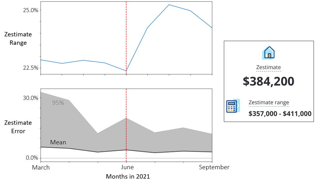
Figure 1: Zillow announced a major update to its Zestimate algorithm on June 15, 2021 (red line). (Top Left) Zillow’s self-reported confidence in its Zestimate (as quantified by the width of the displayed Zestimate range) increased discontinuously from 22.69% (3 months before June 2021) to 24.66% (3 months after June 2021). (Bottom Left) In the same time period (3 months before and after June 2021), empirical average error in the Zestimate (relative to the realized sales price) decreased from 4.36% to 3.41%, and the 95% error in the Zestimate (relative to the realized sales price) decreased from 23.41% to 16.37%. (Right) A snapshot of Zestimate range of 14% ($384,000 $\pm$ 7%) for a home on Zillow.

ML prices that both influences and learn from consumer behaviors are increasingly being used to democratize access to information in a variety of markets (zillow2022zestimate; realtor2022realestimate; forbes2021price; airbnb2022smart; lendingclub2022modelrank; liveart2022estimate). To the best of our knowledge, our work is the first to jointly model the interdependent dynamics of machine learning based-algorithms and consumer behavior. As such, we contribute to the literature on machine learning feedback loops (bottou2013counterfactual; perdomo2020performative; wager2014feedback; sinha2016deconvolving), which does not consider consumer behavior and economic outcomes, and to the literature on dynamic consumer behavior, which does not consider the dynamics of machine learning algorithms. This paper is one of the first (i) to empirically measure the impact of ML pricing on home sale prices (in the context of Zillow and the Zestimate) and (ii) to begin to disentangle Zillow’s proprietary Zestimate algorithm. These two smaller contributions should spark more academic research on and policymaker scrutiny of the dominant role of Zillow’s ML pricing algorithm in the housing market.

More broadly, our work showcases the perils of deploying algorithms that are myopically optimized for statistical objectives such as accuracy, at the expense of long run economic objectives. Such algorithms, as a consequence of feedback loops, could reinforce non-diverse and self-fulfilling preferences (such as recommending fashion content to women and sports content to men, or recommending higher interest rates for loan applications from historically under-served groups due to higher predicted risks). If left unchecked, in the long run, these reinforced preferences could fully diverge from the “ground truth” i.e., preferences in absence of algorithmic interference. We unpack how this divergence from the “ground truth” can make consumers worse off. As such, our work suggests that policymakers monitor and regulate ML pricing. Our work also suggests that intermediary platforms consider the long-term implications of their deployed pricing algorithms when subject to feedback loops. The eventual divergence from ground-truth predicted by our analytical model poses risks to platforms’ reputation and brand perception, which partly depends on the accuracy of their deployed pricing algorithms.

2 Related Literature

A stream of literature has looked at pricing in the housing market before introduction of ML. linneman1986empirical showed a large variance buyers and sellers home value estimates, which is unsurprising given that most buyers and sellers transact infrequently (say, once in 10 years), and, unlike some other assets, houses have a large diversity of features. Field surveys and experimental research tried to estimate valuation errors before the advent of pricing algorithms; error estimates include 14% (goodman1992accuracy), 5.3% (kiel1999accuracy), and 16% (ihlanfeldt1986alternative). One would expect that agents, brokers, and other market experts could correct valuation errors (han2015microstructure), but sellers and expert agents’ contract under information asymmetry. The seller’s inability to observe his agent’s efforts creates a moral hazard in the principal (seller) – agent contract anglin1991residential. When searching (for buyers) is costly, the agent has an incentive to undervalue the home and save on search costs; when the market is competitive, the agent has an incentive to overvalue the home to outbid competing agents. Further, the adverse selection problem prevents the seller from accurately judging whether the agent is knowledgeable about the state of the market. The challenges faced by buyers and sellers in pricing homes is further supported by WakeField research survey (Melcher 2021) which finds that the average US home-buyer tours 15 homes and makes offers on 10 homes, spending a cumulative $845 million of work time on home search and pricing. 85% of first-time buyers say that it is challenging to make offers and stressful to be rejected or outbid.

In this context it is not surprising that ML prices have influence. Participants are likely to find ML pricing attractive because (i) it is free and thus highly accessible, unlike an appraiser; (ii) it seems impartial, unlike agents; and (iii) the platforms (e.g., Zillow and RedFin) report low error rates between ML price and eventual sale price to convey accuracy. Some experts have been highly critical of Zillow’s Zestimate (or Redfins’ Estimate) for being inaccurate, using outdated data, missing local non digitized information and even altogether unusable (houwzer2020zillow). Zillow’s received customer ratings of 3.8, 2.8 and 1.6 on consumeraffairs.com, sitejabber.com and trustpilot.com. Given these concerns we empirically validate that buyers and sellers are in-fact sensitive to changes in Zestimate.

Another stream of literature has looked at feedback loops in a wide range of online learning settings where an ML algorithm learns by making mistakes (barocas2017fairness). Such feedback designs are innocuous in settings where the ML predictions do not contaminate the ground truth label, but elsewhere, the feedback design can slowly accrue a technical debt (sculley2015hidden) that eventually has profound effects (amodei2016concrete). perdomo2020performative identify conditions under which a feedback loop will converge to a stable point. Our analytical framework roughly concurs, but we are less concerned with statistical properties and more concerned with the payoffs at the equilibrium. We discern how much of the covariate distribution shift comes from the evolution of intrinsic housing preferences versus from the ML feedback itself. If the latter dominates, the social surplus may be lost even as the ML algorithm reaches optimal accuracy.

ML feedback loops have been documented in settings such as - ad placement (bottou2013counterfactual), search engine rankings (wager2014feedback) and recommender systems (chaney2018algorithmic; sinha2016deconvolving). Our model of sellers has similarities with the model of (schmit2018human), who assume that users are naïve in believing that ML recommendations are unbiased, and users are myopic and honest about their current action without regard to its impact on future states via the feedback loop. Importantly, in all these examples, individuals interact with ML predictions without an outside option. For example, a user who is seeking relevant search results does not have an alternative mechanism besides the ML algorithm; she cannot realistically achieve the same outcome by interacting with a crowd of her peers. In the housing market, however, buyers and sellers can interact to determine prices in the absence of ML pricing. This interaction may happen indirectly, for example when a seller observes lack of visits or offers from buyers. Thus, the introduction of ML pricing to the housing market is unique in that it replaces the wisdom of the crowd with a single correlated signal. To our knowledge, we are one of the first to evaluate the impacts of ML feedback loops on a market as a whole.

The business literature has identified consequences of ML algorithmic pricing besides the feedback loop. For example, bias propagated by the algorithmic pricing of hotels, car insurance, loans (israeli2020algorithmic), and ride-hailing (pandey2021disparate). (bertini2021pitfalls) find that customers misperceive the motives of firms that offer algorithmic pricing. (assad2020algorithmic) and (brown2021competition) study whether algorithms provide competitive advantages or lead to collusive outcomes. (huang2021seller) identifies settings in which algorithmic pricing may increase market friction. (yu2020algorithmic) argue that algorithmic price might mitigate racial disparities in the housing market. The present paper is unique in this literature because it does not model ML pricing or its statistical properties as static. Instead, we model ML algorithm’s learning in conjunction with the evolving market as both move toward equilibrium.

3 Model

In this section, we model the interdependent evolution of consumer behavior and a machine learning-based pricing algorithm in the context of a housing market. We decompose our model into two components. In the first component, we model how a seller determines the price at which to list their home, buyer offers, the realized sale prices and we define true value of a home (Section 3.1). In the second component, we model how a machine learning-based pricing algorithm estimates home values (Section 3.2). In Section 4, we allow both model components to evolve simultaneously and interdependently, and characterize the equilibrium of the feedback loop between the market and the pricing algorithm.

3.1 First Component: Market Participants

Modeling home-buyers. Consider a home for sale on the market in time period $\tau$. We focus on modeling an “exemplar buyer” of this home: the buyer who has the highest willingness to offer among all buyers interested in this home. Let the willingness to offer of the exemplar buyer be a random variable $y_{\tau}$ drawn from a distribution with mean $\mu$ (assume to be unique for each home) and variance $\sigma_{b}^{2}$ (assumed to be identical across homes), where the variance captures the heterogeneity in buyers’ preferences. Since the seller (the current homeowner) only entertains the highest offer in each time period, it is sufficient to model the exemplar buyer instead of all prospective buyers.

Let the home be listed at price $l_{\tau}$. The exemplar buyer will then offer $\min(y_{\tau},l_{\tau})$, without revealing their willingness to offer $y_{\tau}$. The home sells to the exemplar buyer at the end of time period $\tau$ for $\min(y_{\tau},l_{\tau})=l_{\tau}$ if $y_{\tau}\geq l_{\tau}$, and remains unsold otherwise. We denote by $P(\textrm{sale}|l_{\tau})=P(y_{\tau}\geq l_{\tau};\mu,\sigma_{b}^{2})$ the probability that the home sells in time period $\tau$. While individual buyers can update their valuations during their home search, their aggregate offer distribution $(\mu,\sigma_{b}^{2})$ is assumed to be static.

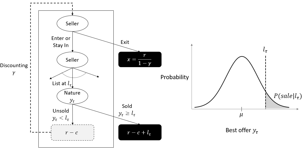
Figure 2: (Left) The home sale process as a single-period game with the seller as the focal agent. The game repeats until the home is sold or the seller decides to exit the market. (Right) A hypothetical distribution of the list price, best offer distribution, and probability of sale.

Modeling home-sellers. Our model of a home-seller is illustrated in Figure 2. At the start of each time period $\tau$, the seller decides whether to list her home for sale, and determines the list price $l_{\tau}$. At the end of the time period, the home (if listed) sells at the list price $l_{\tau}$ with probability $P(\textrm{sale}|l_{\tau})$, based on our model of home-buyers. If the home does not sell at the list price, the seller returns to the decision of whether to continue listing her home for sale. In each time period, the seller earns a flow payoff (regardless of whether or not her home sells) from retaining ownership of the home (such as rental income $r$) less market participation costs $c$ (such as maintaining the home for open-houses). If the seller decides to exit the the market, she receives a lifetime payoff $x$ from retaining ownership of the home (such as via rental income $r$ at discount $\gamma$). We treat this as a terminal state: the seller cannot change her decision to exit the market.

As an example, consider a seller who stays in the market for time periods $1,\dots,T$ and lists her home at a sequence of prices ${l_{1},...,l_{\tau},...,l_{T}}$, until her home sells in period $T$. Her payoff $\pi$ and the outside option value $x$ (had she not entered the market at all) are given by,

$$\pi=\frac{1-\gamma^{T}}{1-\gamma}\times(r-c)+\gamma^{T}\times l_{T}\text{ \quad; \quad}x=\frac{r}{1-\gamma}$$ (1)

The seller enters the market if her estimate of the expected payoff $\tilde{\mathbb{E}}[\pi]$ is greater then the outside option value $x$. The expectation $\tilde{\mathbb{E}}[\pi]$ is over all possible realizations of sale prices, on-market durations, and whether or not the home sells. The seller lists her home at the optimal price $l_{\tau}^{*}$ at the beginning of every period $\tau$ to maximize her expected payoff $\tilde{\mathbb{E}}[\pi|l_{\tau}]$ from period $\tau$ onwards.

We use the notation $\tilde{\mathbb{E}}[\cdot]$ to distinguish between the seller’s estimate of the expected payoff and the actual expected payoff $\mathbb{E}[\cdot]$. The seller’s estimate of the expected payoff depends on her estimate of the sale probability $\tilde{\mathbb{P}}(\textrm{sale}|l_{\tau})$, which in turn depends on her estimate of the offer distribution parameter $\tilde{\mu}_{\tau}$ in period $\tau$. The seller also has some uncertainty (variance) about her estimate, which we denote by $\sigma^{2}_{s,\tau}$. The seller’s uncertainty and the estimation errors arising from $\tilde{\mu}_{\tau}\neq\mu$, $\tilde{\mathbb{P}}(\textrm{sale}|l_{\tau})\neq\mathbb{P}(\textrm{sale}|l_{\tau})$, and $\tilde{E}[\pi|l_{\tau}]\neq E[\pi|l_{\tau}]$) will lower payoffs, which platforms like Zillow attempt to alleviate with their machine learning-based pricing algorithms.

We denote the seller’s initial estimates as $\tilde{\mu}=\tilde{\mu}_{\tau=0}$ and $\sigma_{s}^{2}=\sigma^{2}_{s,\tau=0}$. In each subsequent time period $\tau$, the seller learns and updates her initial estimates and uncertainty ($\tilde{\mu}_{\tau},\sigma^{2}_{s,\tau}$). We model these updates as a Bayesian learning process in which the seller combines her current estimate $(\tilde{\mu}_{\tau},\sigma^{2}_{s,\tau})$ with the observable market signal $(\mu,\sigma^{2}_{\textrm{signal}})$ to develop an updated estimate $(\tilde{\mu}_{\tau+1},\sigma^{2}_{s,\tau+1})$. The market signal is observed when the seller interacts with prospective buyers, some of whom implicitly of explicitly reveal the price they are willing to offer for the seller’s home. We assume that the market signal is noisy, but unbiased with respect to the buyer’s offer distribution parameter $\mu$. With time on the market, we assume that the seller’s estimate of $\mu$ improves and her uncertainty reduces: $\tilde{\mu}_{\tau}\rightarrow\mu,\sigma^{2}_{s,\tau}\rightarrow 0$ as $\tau\rightarrow\infty$.

Home values. Intuitively, a home’s value $v$ is its market clearing price. This is easy to formalize for, say, a single IBM stock, with millions of identical units transacted among thousands of buyers and sellers every day. In contrast, a single home is bought and sold only a few times in many years. Hence, we consider a thought experiment where the same home is sold thousands of times. The value of the home $v$ in this thought experiment is its sale price $p$ (which depends on the buyer offer distribution and the seller’s estimate of this parameter) averaged over all the times it is sold:

$$v=\mathbb{E}[\mathbb{E}[p|\mu,\tilde{\mu},\sigma_{b},\sigma_{s},\sigma_{signal}]]$$ (2)

Next we will consider machine learning based estimation of this home value. Note that the machine learning algorithm does not model the market structure (offers $(\mu,\sigma_{b})$, beliefs $(\tilde{\mu},\sigma_{s}$, and signals $\sigma_{signal}$).

3.2 Second Component: Machine Learning-Based Pricing Algorithm

We assume that the home value $v_{k,t}=G_{t}(\mathbf{X}_{k})$ of a home $k$ at time $t$ is a time-evolving function of the home’s characteristics $\mathbf{X}_{k}$. This can be interpreted as home buyers’ preferences for the home’s characteristics evolving over time, while the home’s characteristics remain unchanged. We further assume that the resulting home value evolves as a random walk:

$$v_{k,t}=v_{k,t-1}+e^{\textrm{rw}}_{k,t},\qquad v_{k,t}=G_{t}(\mathbf{X}_{k}),~{}e^{\textrm{rw}}_{k,t}\sim N(0,\sigma^{2}_{\textrm{rw}})$$ (3)

In this section, we propose a general machine learning framework for home value estimation. For analytical simplification we assume that the machine learning model parameters $\theta_{t}$ are retrained every period $t$ to approximate the underlying true home preferences $G_{t}(\mathbf{X}_{k})$. Finally we derive analytical expressions for the machine learning-based prices as a function of observed sale prices.

General machine learning framework. Our framework assumes that the machine learning model of home values is trained to (i) accurately estimate the value of each home in the training data, and (ii) estimate similar home values for homes with similar features. Satisfying objective (i) increases in-sample accuracy, but decreases out-of-sample accuracy due to over-fitting. Essentially, the inclusion of objective (ii) regularizes the model to increase its generalization power. Our framework is a generalization of the network lasso framework (hallac2015network) to non-convex optimization objectives.

Formally, let $\mathcal{H}_{t}$ be a set of $N$ homes used to train the machine learning model at time $t$. For each home $k\in\mathcal{H}_{t}$, let $v_{k,t}$ be the true value of the home at time $t$, and $\mathbf{X}_{k}\in\mathbb{R}^{\bar{Q}}$ be a $\bar{Q}$-dimensional vector of the home’s characteristics (such as its number of bedrooms and year of construction). We assume that the machine learning model parameters $\theta_{t}$ are given by:

$$\theta_{t}=\textrm{argmin}_{\theta}~{}\left[~{}\underbrace{\sum_{k\in\mathcal{H}_{t}}f_{k}(\mathbf{X}_{k}|\theta)}_{\textrm{objective (i)}}\quad+\quad\underbrace{\sum_{m,n\in\mathcal{H}_{t}}g_{mn}(\mathbf{X}_{m},\mathbf{X}_{n}|\theta)}_{\textrm{objective (ii)}}~{}\right]~{}$$ (4)

Here, $f_{k}(\mathbf{X_{k}}|\theta)$ is a loss function capturing the first objective of accurate in-sample estimation for each home $k\in\mathcal{H}_{t}$ in the training data, and $g_{mn}(\mathbf{X_{m}},\mathbf{X_{n}}|\theta)$ is a loss function capturing the second objective of making similar estimations for similar homes. Note that we make no assumptions about the functional form of either loss function, or about the architecture of the machine learning model. As such, our framework generalizes a variety of common machine learning models, including deep neural networks.

Example. As a specific example of our framework, let $\hat{v}_{k}=F(\mathbf{X}_{k},\Theta_{k})$ be the estimated price of each home $k$ derived using a neural network $F(\cdot)$ with weights $\Theta_{k}$. While the weights are different for each home $k$, a single neural network $F(\cdot)$ is trained to learn the weights $\Theta_{1},\dots,\Theta_{N}$ of all $N$ homes in the training data $\mathcal{H}_{\tau}$; these weights can be viewed as homes’ embeddings. To maximize in-sample accuracy, we minimize the mean squared error by setting $f_{k}(\mathbf{X_{k}}|\theta)=[\hat{v}_{k}-v_{k,t}]^{2}=[F(\mathbf{X}_{k},\Theta_{k})-v_{k,t}]^{2}$. To improve out-of-sample accuracy, we penalize differences between the learned weights for pairs of similar homes. Specifically, we set $g_{mn}(\mathbf{X}_{m},\mathbf{X}_{n}|\theta)=\lambda\|\mathbf{X}_{m}-\mathbf{X}_{n}\|_{2}\|\Theta_{m}-\Theta_{n}\|_{2}$, where $\|\cdot\|$ is the Euclidean distance or $L_{2}$ norm, and $\lambda$ is a regularization hyperparameter. Note that the parameters $\theta=\{F(\cdot),\lambda\}\cup\{\Theta_{k}\}_{k\in\mathcal{H}_{t}}$ include the neural network architecture $F(\cdot)$, the regularization hyperparameter $\lambda$, and the weights $\Theta_{k}$ for each home $k\in\mathcal{H}_{t}$.

Regularization and home clustering. Solving for $\theta_{\tau}$ in Eq. 4 essentially performs joint home value estimation and home clustering, where a pair of homes $i,j$ with similar learned weights $\Theta_{i},\Theta_{j}$ can be assigned to the same cluster by discretizing the weight values (by rounding them to the nearest integer, for example). After discretization, $Q$ homes in a cluster $\mathcal{C}_{i}$ for $i=1,\dots,Q$ have the same learned weights $\Theta_{k}$ and similar characteristics $\mathbf{X}_{k}$ (and hence, similar estimated home values). The regularization parameter $\lambda$ controls the clustering granularity: $\lambda=0$ permits each home to form its own cluster, while $\lambda\rightarrow\infty$ leads to a single cluster containing all homes in the training data. We denote by $Q$ the number of clusters, and assume (for analytical simplification) that each cluster contains exactly $N/Q$ homes.

Generating algorithmic prices. The clustering of homes facilitates making out-of-sample predictions. Let $\bar{\mathbf{X}}_{\mathcal{C}}$ denote the centroid of cluster $\mathcal{C}$ (the average of $\mathbf{X}_{k}$ over all homes $k\in\mathcal{C}$), and let $\bar{v}_{\mathcal{C},t}$ be the average value of all homes $k\in\mathcal{C}$ at time $t$. We assign each out-of-sample home $q$ with characteristics $\mathbf{X}_{q}$ to its nearest cluster $\mathcal{C}(q)\in\{\mathcal{C}_{1},\dots,\mathcal{C}_{J}\}$ with the smallest Euclidean distance $\|\mathbf{X}_{q}-\bar{\mathbf{X}}_{\mathcal{C}}\|_{2}$, and could subsequently use $\bar{v}_{\mathcal{C}(q),t}$ as its predicted home value. However, true home values are unobservable in practice. Hence, a common proxy for home values is their sales price, which are observable in the past. Using this proxy plays an important role in the machine learning errors that we discuss later in this section. Let $p_{k,t}$ be the sale price of home $k$ at time $t$, and let $\bar{p}_{\mathcal{C},t}$ be the average sale price of all homes in cluster $\mathcal{C}$. Then the predicted price of an out-of-sample home $q$ assigned to cluster $\mathcal{C}(q)$ (as described above) at time $t+1$ is given by:

$$z_{q,t+1}=\bar{p}_{\mathcal{C}(q),t}=\frac{Q}{N}\times\sum_{k\in\mathcal{C}(q)}p_{k,t}$$ (5)

Table 1: Assumptions about the distributions in our simple and full models.

	Simple Model	Full Model
Buyer Offer Distribution $P(y_{\tau})$	$U[\mu-\sigma,\mu+\sigma]$	$N(\mu,\sigma_{b}^{2})$
Seller Estimate $P(\tilde{\mu})$	$P(\tilde{\mu}=\mu-2\sigma)=P(\tilde{\mu}=\mu)=P(\tilde{\mu}=\mu+2\sigma)=1/3$	$N(\mu,\sigma_{s}^{2})$
Seller Learning $\sigma_{\textrm{signal}}^{2}$	0	$\kappa\sigma_{b}^{2}$

Table 2: Table of notation and definitions

Exogenous Variables

Notation	Description
$v_{t}$	True value (market clearing price) of home at time $t$
$\sigma_{rw}^{2}=Var_{t}[v_{t+1}-v_{t}]$	Variance of true value changes of a home over time.
$\sigma_{v}^{2}=Var_{k}[v_{t}]$	Variance of true value across all homes in one period.
$\sigma_{e}^{2}=Var_{i}[\tilde{v}_{i,t}-v_{t}]$	Variance of participant $i$ valuations (before introducing ML)
$N$	Total number of homes sold in one period.

Key Endogenous Variables

Notation	Description
${l_{\tau}}_{t}$	Sequence of list prices set by seller for home at time $t$
$p_{t}$	Realized sale price
$\tilde{v}_{i,t}$	Participant $i$ valuation of home at time $t$
$z_{t}$	ML (Machine Learning) price of home at time $t$
$Q$	ML model hyperparameter controlling number of clusters

Outcomes Variables (as function of reliance $\alpha$)

Notation	Description
$\alpha(\hat{\sigma}^{2}_{z})$	Participant reliance on ML price
$\sigma^{2}_{z}(\alpha)$	True ML price error ($\sigma^{2}_{z}(\alpha=0)$ denoted by $\sigma^{2}_{z}$)
$\hat{\sigma}^{2}_{z}(\alpha)$	Estimated ML price error ($\hat{\sigma}^{2}_{z}(\alpha=0)$ denoted by $\hat{\sigma}^{2}_{z}$)
$\pi,\Pi(\alpha)$	Realized payoff and expected risk averse payoff

4 Results

In Section 3.1, we described our model of buyer-seller interactions grounded in the structure of the housing market — the offer distribution parameters ($\mu,\sigma_{b}^{2}$), the seller’s estimate of the offer distribution mean $\tilde{\mu}$, her uncertainty $\sigma^{2}_{s}$, the seller’s learning aided by a market signal $(\mu,\sigma^{2}_{\textrm{signal}})$, and the seller’s outside option value $x$ and market participation costs $c$. We further formalized the sellers’ optimal listing price choice $l_{\tau}$ in terms of these parameters. However, a signal such as the ML price $z$ does not convey information about the offer distribution $\mu$ or the list price $l_{\tau}$, nor is it tailored to an individual sellers characteristics. Instead, the ML price $z$ is an estimate of a home’s value $v$ (equation 2) summarized over these market structure details and individual heterogeneity.

In section 4.1, we derive the home value $v$ and distribution of sale prices ($E[p],Var[p]$). We consider two sets of assumptions (listed in Table 1) about the distributions of offers $y_{\tau}$, the seller’s estimate $\tilde{\mu}_{\tau}$, and the market signal $\sigma_{\textrm{signal}}^{2}$. In our results described in Section 4, we use the “simple” model for analytical closed-form solutions. In Appendix B.2, we employ numerical simulations under the “full” model to verify that our findings are consistent with the “simple” model. In section 4.2, we will derive machine learning pricing errors (true $\sigma_{z}^{2}=Var[v-z]$ and estimate $\hat{\sigma}_{z}^{2}=Var[p-z]$). In section 4.3, we will identify equilibrium of the feedback loop between the machine learning pricing error estimate $\hat{\sigma}_{z}^{2}(\alpha)$ and reliance on machine learning prices $\alpha(\hat{\sigma}_{z}^{2})$ which depend on each other. Finally, in section 4.4, we will use these equilibrium expressions to formulate payoffs for sellers at the equilibrium. Table 2 and 3 summarize the notation and key results.

4.1 Home Value and Sale Prices

Consider an oracle who knows a home’s true offer distribution ($\mu,\sigma_{b}^{2}$), and knows that the sellers have potentially erroneous estimates. The oracle could calculate the home’s value $v(\mu)$ by integrating over the sellers’ estimates of the buyer offer distribution $\tilde{\mu}$, and over the stochasticity in buyers’ offers (embedded in $\mathbb{E}[p|\mu,\tilde{\mu}]$), as follows:

$$v(\mu)=\mathbb{E}[\mathbb{E}[p|\mu,\tilde{\mu}]]=\int_{\tilde{\mu}}P(\tilde{\mu}|\mu,\sigma)\times\mathbb{E}[p|\mu,\tilde{\mu}]$$ (6)

Similarly, we can formalize the seller’s estimate $\tilde{v}$ of her home’s value in time period $\tau$ (where we drop the subscript $\tau$). The seller does not know her home’s true offer distribution ($\mu,\sigma_{b}^{2}$), However, the seller knows that her estimate $\tilde{\mu}$ is drawn from a distribution with mean $\mu$ and variance $\sigma^{2}_{s}$. The seller’s valuation of her home $\tilde{v}$ is then given by $\tilde{v}=\tilde{\mathbb{E}}[v(\mu)]$, where the expectation is over all possible estimates of $\mu$ by the seller. Now consider an external signal from an ML price $z$ that also claims to estimate the home’s value: $z=\hat{E}[p]=\hat{v}$, where we use $\hat{E}[\cdot]$ to differentiate between the algorithm’s estimate and the seller’s estimate (denoted by $\tilde{\mathbb{E}}[\cdot]$). After observing this signal, the seller updates their valuation $\tilde{v}$ by combining their prior valuation (before observing and independent of the ML price) and the ML price $z$ as follows:

$$\tilde{v}=(1-\alpha)\times\tilde{\mathbb{E}}[v(\mu)]+\alpha\times z\quad;\quad\textrm{Var}[\tilde{v}]:=(1-\alpha)^{2}\textrm{Var}[\tilde{v}]$$ (7)

This formulation for impact of ML price $z$ condenses complex details on how sellers absorb the ML price $z$. The seller (jointly with their agent) receives informative signals from a lot of sources (agent, appraisers, neighbors and market experts) all embedded into their private valuation $\tilde{\mathbb{E}}[v]$. The ML price $z$ is yet another informative signal, specially treated in our model because we want to isolate its impact, to construct a final valuation $\tilde{v}$. The seller uses the valuation ($\tilde{v}$ e.g., $520k) to infer likely offers ($\tilde{\mu}\pm\sigma_{b}$ e.g., $500k to $550k) and a corresponding good list price ($l^{*}$ e.g., $540k). A similar influence occurs for buyers. Individual buyers (jointly with any buyer agent) incorporate ML price $z$ as yet another informative signal into constructing a valuation $\tilde{v}$. This in turn updates individual buyers’ willingness to offer and consequently the offer distribution from the exemplar buyer every period $\mu$. We do not explicitly model the estimation and willingness to offer for individual buyer. But implicitly the ML price $z$ impacts valuations of both buyers and sellers, and thereby impacts the realized sale price $p$. Going forward we will use the phrase buyer-seller when discussing impact of ML price.

Using the definitions above, we can derive expressions for home value $v$, buyer-seller valuation $\tilde{v}$ and the sale price $p$ .

Lemma 1

The true home value $v$ is given by,

$$v=(\mu+2\sigma/3-\sqrt{2c\sigma})$$ (8)

Each seller’s valuation (and the variance of this valuation) is given by,

$$\tilde{v}(\alpha=0)=\tilde{\mathbb{E}}[p|z]=\tilde{\mu}+2\sigma/3-\sqrt{2c\sigma}\text{ ; \quad}\sigma_{e}^{2}(\alpha=0)=\sigma_{e}^{2}=Var[\tilde{v}]=8\sigma^{2}/3$$

$$\tilde{v}(\alpha)=(1-\alpha)\times\Big{(}\tilde{\mu}+2\sigma/3-\sqrt{2c\sigma}\Big{)}+\alpha\times z\text{ ; \quad}\sigma_{e}^{2}(\alpha)=(1-\alpha)^{2}\sigma_{e}^{2}$$ (9)

The distribution of sale price is given by,

$$\mathbb{E}[p|z]=(1-\alpha)\times\Big{(}\mu+2\sigma/3-\sqrt{2c\sigma}\Big{)}+\alpha\times z\text{ ; \quad}\sigma_{\epsilon}^{2}(\alpha)=Var[p]=\delta\sigma_{e}^{2}(\alpha)\text{ ; \quad}\delta=(1/6)$$ (10)

Reliance on ML price ($\alpha>0$) adds bias in valuations and sale prices i.e., $v\neq\mathbb{E}[p]=\mathbb{E}[\tilde{v}]$ if $z\neq p$. It also reduces variance in valuations and sale prices i.e., $Var[p]$ and $Var[\tilde{v}]$ are decreasing in $\alpha$.

Let the subscript $i$ index each seller. We can express each seller’s valuation as $\tilde{v}=\mathbb{E}[\tilde{v}_{i}]+e_{i}$ where $e_{i}=(1-\alpha)(\tilde{\mu}-\mu)$ is the noise in valuation across individual sellers with $E[e_{i}]=0$. We can also express the realized sale price as $p=\mathbb{E}[p]+\epsilon$ where $\epsilon$ is the noise in realized sale prices (across multiple hypothetical sale instances) with $E[\epsilon]=0$. There are two intermediate results worth highlighting here. First, the true expected sale price is equal to the expected seller valuation: $\mathbb{E}[p]=\mathbb{E}[\tilde{v}_{i}]$. At $\alpha=0$ we have $v=\mathbb{E}[p]=\mathbb{E}[\tilde{v}_{i}]$ i.e., prior valuations (before observing ML price) are unbiased with respect to the true value $v$. At $\alpha>0$, the valuation are not unbiased anymore i.e., $\mathbb{E}[\tilde{v}_{i}]\neq v$ if $z\neq p$. Second, the variance in sale prices $Var[p]$ is proportional to variance (disagreement) of seller’s valuation $Var[\tilde{v}]$. The constant $\delta$ can be interpreted as the degree to which disagreement in private valuations is reduced by participating in the market (buyers and sellers learning and attaining consensus). The variance in valuations $Var[\tilde{v}]$, and consequently variance in sale prices $Var[p]$ are diminished by a fraction $(1-\alpha)^{2}$. So overall, ML price is adding some bias but removing some variance from valuations and sale prices. The payoff implications of this will be expressed in Lemma 2 and Lemma 3 in section 4.4.

4.2 Machine Learning Pricing Errors

We can use equations 5 (ML price $z$ as function of sale prices $p$), and Lemma 1 (sale prices $p$ as function of ML price $z$) to formulate the feedback loop. Figure 3 visually illustrates this loop. In this section, we will start by calculate the true Machine Learning pricing errors $\sigma_{z}^{2}=Var[v-z]$ and its empirical estimate $\hat{\sigma}_{z}^{2}=Var[p-z]$ (because true value $v$ is not observed, only sale prices $p$ are observed).

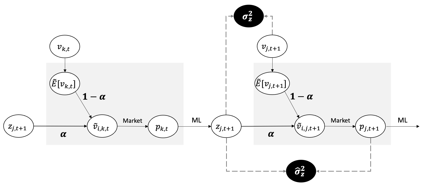
Figure 3: Buyer-seller $i$ of home $k$ construct home valuation $\tilde{v}_{i,k,t}$ using ML price $z_{k,t}$ and private estimation with weights $\alpha$ and $1-\alpha$ respectively. The market interaction among buyer-sellers with similarly constructed valuations produces a sale prices $p_{k,t}$. $N$ home sales similar to home $k$ form training sample for Machine Learning model. In the next period, a home $j$ is influenced by ML price $z_{j,t+1}$. The machine learning error can be estimated $\hat{\sigma}_{z}^{2}$ using ML price $z_{j,t+1}$ and realized sale price $p_{j,t+1}$. This is an approximation since the true home value $v_{j,t+1}$ is not observed.

Table 3: At a glance view of Lemma and Propositions

Lemma 1	Expression for home value and sale price distribution
Lemma 2	Expression for expected payoff
Lemma 3	Expression for variance of payoffs
Proposition 1	Confounded ML error is inflated i.e., $\sigma^{2}_{z}(\alpha)\geq\sigma^{2}_{z}(\alpha=0)$
Proposition 2	Confounded ML error estimate is deflated i.e., $\hat{\sigma}^{2}_{z}(\alpha)\leq\sigma^{2}_{z}(\alpha)$ if $\alpha$ large enough
Proposition 3	Confounded ML error estimate $\hat{\sigma}^{2}_{z}(\alpha)$ is decreasing in $\alpha$ if $\alpha$ large enough
Proposition 4	Proposition 2 and 3 always true at equilibrium $\alpha^{*}$
Proposition 5	$\alpha^{*}=1$ always an equilibrium and only equilibrium if $\sigma_{z}^{2}/\sigma_{e}^{2}$ is small enough
Proposition 6	Variance in payoff $Var[\pi]$ increasing in $\alpha$ if $\alpha$ is large enough
Proposition 7	Risk averse payoff $\Pi(\alpha^{*}=1)<\Pi(\alpha=0)$ if $\sigma_{z}^{2}/\sigma_{e}^{2}$ is large enough

The ML price $z_{k,t+1}$ for a focal home $k$ is given by $z_{k,t+1}=\bar{p}_{K,t}$ from equation 5, where $K=\mathcal{C}(k)$ is the focal home’s peer cluster at time $t$. We now focus on the focal home $k$ and drop the subscript $k$. The error in ML price is the difference between the actual realized home value $v_{t+1}$ and ML price $z_{t}$. This error can be decomposed into three components as,

$$v_{t+1}-z_{t+1}=\underbrace{v_{t+1}-v_{t}}_{\text{Random Walk}}+\underbrace{v_{t}-v_{K,t}}_{\text{Unpriced Features}}+\underbrace{v_{K,t}-\bar{p}_{K,t}}_{\text{Finite Sample Error}}$$ (11)

Home values in the current period $v_{t}$ can not forecast the random walk of preferences and values into the next period $v_{t+1}$. We denote variance of random walk error as an exogenous and constant quantity $Var[v_{t+1}-v_{t}]=\sigma^{2}_{rw}$.

We can interpret the clustering of homes into $Q$ clusters (described in Section 3.2) in terms of matching on homes’ features (home characteristics such as its age and size). Specifically, given a total number of features $\bar{Q}$, we can view the homes within a cluster as being identical or matching on $Q$ features. In using the peer cluster’s mean sale price, $\bar{Q}-Q$ unique features of the focal home are left unpriced i.e., an error $v_{t}-v_{K,t}$. Intuitively, the variance of unpriced features should depend on variance of all features and the number of priced features $Q$. The variance of all features, also the heterogeneity in housing stock, $\sigma^{2}_{v}$ is treated as an exogenous constant. The choice of priced features $Q$ explains increasingly greater proportion of the total variance. This is captured by monotonically decreasing function $h(Q)$ (possibly with positive second derivative because of diminishing returns). Thus we have $Var[v_{t}-v_{K,t}]=h(Q)\times\sigma^{2}_{v}$. Intuitively, as the number of “clustering features” (features used to place homes in the same cluster) increases, clusters will have fewer, very similar homes. Hence, the variance of home values in a cluster will be low. Similarly, as the number of “clustering features” decreases, clusters will have more, dissimilar homes. Hence, the variance of home values in a cluster will be high.

The ML price is effectively the sample mean of cluster sale prices. The finite sample error is the difference between the mean of cluster sale prices and the true cluster value i.e., $v_{K,t}-\bar{p}_{K,t}$. Since there are $N/Q$ home sales in the cluster, we can express $\bar{p}_{K,t}$ as,

$$\bar{p}_{K,t}=(Q/N)\times\sum_{k}\Big{[}p_{k,t}\Big{]}$$

$$=(Q/N)\times\sum_{k}\Big{[}\mathbb{E}[v_{i,k,t}]+\epsilon_{k,t}\Big{]}$$

$$=(Q/N)\times\sum_{k}\Big{[}\mathbb{E}[(1-\alpha)\times\tilde{v}_{i,k,t}+\alpha\times z_{k,t}]+\epsilon_{t}\Big{]}$$

$$=(Q/N)\times\sum_{k}\Big{[}(1-\alpha)\times v_{k,t}+\alpha\times(v_{k,t}+e^{z}_{k,t})+\epsilon_{k,t}\Big{]}$$

$$=(Q/N)\times\sum_{k}\Big{[}v_{k,t}+\alpha e^{z}_{k,t}+\epsilon_{k,t}\Big{]}$$

$$=v_{K,k,t}+\alpha(Q/N)\times\sum_{k}e^{z}_{k,t}+(Q/N)\times\sum_{k}\epsilon_{k,t}$$ (12)

Note that under $\alpha=0$, the second components disappears. Under $\alpha>0$, this additional component captures the confounding of the sale price from the ML price.

We can now express the variance of the finite sample error as,

$$Var[v_{K,t}-\bar{p}_{K,t}]=Var\Big{[}(Q/N)\times\sum_{k}(\alpha\mathbb{E}[e^{z}_{k,t}]+\epsilon_{k,t})\Big{]}$$

$$=\alpha^{2}Var[(Q/N)\times\sum_{k}e^{z}_{k,t}]+Var[(Q/N)\sum_{k}\epsilon_{k,t}]$$

$$=\alpha^{2}Q\sigma_{z}^{2}/N+\delta Q(1-\alpha)^{2}\sigma^{2}_{e}/N$$ (13)

We can now write the full ML price error variance as,

$$\sigma_{z}^{2}(\alpha)=Var\Big{[}(v_{t+1}-v_{t})+(v_{t}-v_{K,t})+(v_{K,t}-\bar{p}_{K,t})\Big{]}$$

$$=\sigma^{2}_{rw}+h(Q)\times\sigma^{2}_{v}+\alpha^{2}Q\sigma_{z}^{2}(\alpha)/N+(1-\alpha)^{2}\delta Q\sigma^{2}_{e}/N$$

$$=\Big{(}\frac{1}{1-Q\alpha^{2}/N}\Big{)}\times(\sigma^{2}_{rw}+h(Q)\times\sigma^{2}_{v}+(1-\alpha)^{2}\delta Q\sigma^{2}_{e}/N)$$

$$=\sigma^{2}_{rw}+h(Q)\times\sigma^{2}_{v}+(1-\alpha)^{2}\delta Q\sigma^{2}_{e}/N$$ (14)

The denominator $(1-Q\alpha^{2}/N)$ is very close to 1 since $Q<<N<<\infty$ and set to 1 going forward as a conservative assumption for analytical simplification. The ML error is increasing in random walk of home preferences $\sigma^{2}_{rw}$, heterogeneity in housing stock $\sigma^{2}_{v}$ and error in private valuations $\sigma^{2}_{e}$. The ML error sensitivity to $Q$ is mixed - the unpriced feature error component $h(Q)\times\sigma^{2}_{v}$ is decreasing in $Q$ while the finite sample error component $(1-\alpha)^{2}\delta Q\sigma^{2}_{e}/N$ is increasing. We will discuss endogenization of $Q$ later in this section. The ML error is increasing in $\alpha$. In fact, we can express the ML error in terms of the un-confounded ML error $\sigma_{z}^{2}=\sigma_{z}^{2}(\alpha=0)$ as,

$$\sigma_{z}^{2}(\alpha)=\sigma_{z}^{2}+\alpha(2-\alpha)\delta Q\sigma^{2}_{e}/N$$

$$\text{where \quad}\sigma_{z}^{2}=\sigma_{z}^{2}(\alpha=0)=\sigma^{2}_{rw}+h(Q)\times\sigma^{2}_{v}+\delta Q\sigma^{2}_{e}/N$$ (15)

The un-confounded ML error $\sigma_{z}^{2}$ are valid in a limited setting where the platform does not reveal the ML price or the buyers-sellers do not use the ML price at all. In the rest of the paper, we will continue to compare confounded results at $\alpha>0$ with unconfounded results at $\alpha=0$ to highlight impact of the confounding over the feedback loop. In comparing expressions for confounded ($\sigma_{z}^{2}(\alpha>0)$) and unconfounded ($\sigma_{z}^{2}=\sigma_{z}^{2}(\alpha=0)$) ML errors, the additive term $\alpha(2-\alpha)\delta Q\sigma^{2}_{e}/N$ captures the amplification in ML error because of the confounding.