tcb@breakable

Pulse in collapse: a game dynamics experiment

Abstract

The collapse process is a constitutional sub-process in the full finding Nash equilibrium process. We conducted laboratory game experiments with human subjects to study this process. We observed significant pulse signals in the collapse process. The observations from the data support the completeness and the consistency of the game dynamics paradigm.

Contents

1. 1 Introduction
   1. 1.1 Collapse
   2. 1.2 Research questions
   3. 1.3 Outline
2. 2 Game and the prediction
   1. 2.1 Game design
   2. 2.2 Classical game theory predictions
   3. 2.3 Game dynamics theory prediction
   4. 2.4 Game experiment
3. 3 Results
   1. 3.1 Distribution
   2. 3.2 Eigencycle
   3. 3.3 Collapse
   4. 3.4 Model comparison
4. 4 Discussion and conclusions
   1. 4.1 Implications
   2. 4.2 Related works
   3. 4.3 Conclusion
5. A
   1. A.1 Abbreviations
   2. A.2 Distribution
   3. A.3 Cycle
      1. A.3.1 Verify the statics
      2. A.3.2 Verification of the dynamics theory
   4. A.4 Collapse
      1. A.4.1 Measurement definition
      2. A.4.2 Data
   5. A.5 The game dynamics paradigm and its workflow

1 Introduction

Game equilibrium finding is a process [18, 25, 8, 13]. This process is also referred to as evolution, or adjustment process, or deviation from equilibrium process, or the convergence process in game theory and experiment. It is a non-linear spontaneous evolution process driven by game participates’ strategic interactions.

In the study of game theory, terms such as adjustment dynamics [18], learning theory [12], population game dynamics, evolutionary game theory [10, 26] or market dynamics [23], are related to this the process. These terms are included in the game dynamics paradigm.

As a scientific paradigm that moves beyond equilibrium theory (classical game theory, or game statics theory), the game dynamics paradigm is expected to be able to describe the regularity of the game dynamic process in terms of completeness and consistency, as well as reality and accuracy [25, 8, 13].

Instead of using the statics theory to study the predictable equilibrium (stable statistical relationships among strategy), game dynamics theory studies the predictable motion (temporary deviations from equilibrium). For example, in the rock-paper-scissors game [33, 6, 39, 38], the persistent cycle is a style motion pattern of predictable temporary deviation from equilibrium (PTDE). Such a pattern can be exploited [11]. In real life, most high-frequency trading strategies which are not fraudulent, but instead exploit the PTDE [36].

Following this paradigm, we investigate an unignorable sub-process of the full finding Nash equilibrium process. In this section, we introduce the sub-process, namely collapse process; then, we introduce the research questions and offer a summary of the contents of this paper.

1.1 Collapse

A real game system can involve a large number of strategies, most of which would be dominated during the process of finding Nash equilibrium [3, 22]. As illustrated in Figure 1(a), the full equilibrium finding process can be classified into three stages:

1. In the initial stages, having no information about the game, agents randomly choose a strategy vector from the strategy space for optimal payoff. During this period, the game’s social evolution trajectory is highly stochastic, smoothly distributed throughout the full game space.

2. Later, in the period of infancy, each agent may start to identify their own nonprofit strategy by learning from strategy interactions. As a result, the dimensions of the game strategy space may collapse. In theory, ‘a dominated strategy can dominate a domination before being dominated’, meaning that a phenomenon known as a pulse could exist. A conceptual rendering of a pulse in the collapse process is shown in Figure 1(b).

3. Finally, when there is no dominant strategy, the evolution trajectory will converge to a fixed pattern (a persistent cycle or fixed equilibrium point) of the game. When rendered as an image, the pattern is the same as a condensed structures in astrophysics.

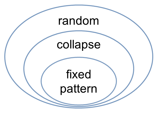
(a)

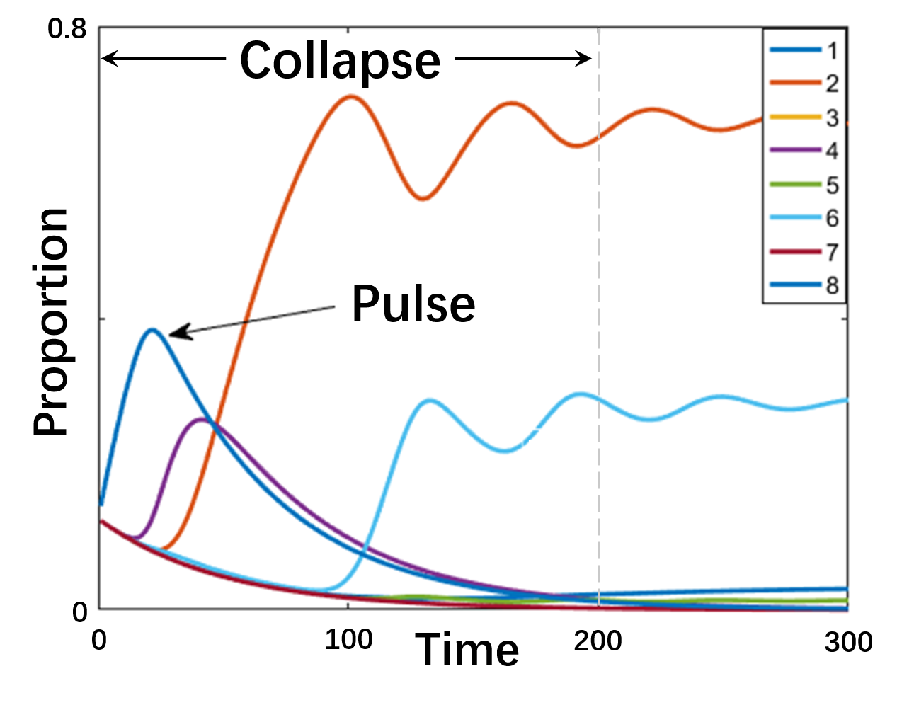
(b)

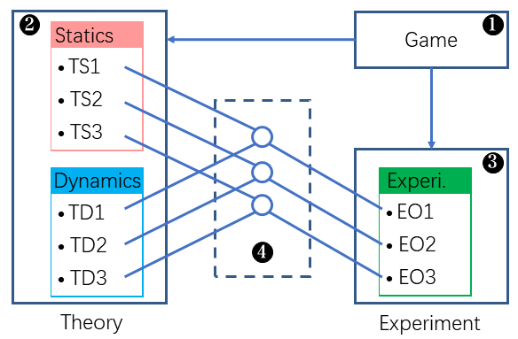
(c)

Figure 1: Conceptual figure. (a) The three periods in the full Nash-equilibrium-finding process, moving from random to collapse to fixed pattern. This study focus on the collapse process. (b) An illustration of a pulse in a collapse.(c) The workflow of this report: The Game, Theory (Static and Dynamic) vs. Experiment by Observations (1-distribution; 2-cycle; 3-collapse). For the abbreviations, see Table A1.

The collapse appears in the second stage. The term ‘collapse’, introduced to game dynamics here, is borrowed from the concept of ‘gravitational collapse’ in astrophysics [35] which is a fundamental mechanism and a legitimate constituent part of the formation of structures in the universe. This study benefits from the physical pictures in astrophysics.

1.2 Research questions

We investigate the collapse process by asking the following two questions:

• In controlled laboratory game experiments with human subjects, can significant new observations be obtained during a collapse process?

• Can the existing game theory paradigm consistently and completely capture the collapse process?

Answering these questions is not trivial, for the following reasons:

• From a scientific perspective, without evidence from the collapse process, our knowledge of the full equilibrium-finding process is obviously incomplete.

• Within a scientific paradigm, without conducting experiments on collapses, there is no basis for the reality of the theory [16, 15, 21].

These issues relate to reality and accuracy, as well as to the completeness and consistency of the game dynamics paradigm, and are therefore not trivial.

1.3 Outline

To answer our research questions, following the experimental game theory paradigm [23, 4, 6, 39, 29, 2], we carried out the workflow shown in Figure 1(c):

• We designed a parameterised three card poker game for use in a laboratory study of the the statics theory and the dynamics theory (see section 2.1).

• We derived the predictions for three variables (distribution, cycle, and pulse) by the statics theory and the dynamics theory (see sections 2.2 and 2.3).

• We conducted laboratory experiments which include 3-treatments with 72 human subjects, fixed-paired, and 1000 repeated games (see section 2.4).

• We outlined the experimental observations and their theoretical verification of the three variables (distribution, cycle, and pulse in sections 3.1, 3.2 and 3.3, respectively). Additionally, we we report the results of comparing the models (see section 3.4).

In the discussion section, we offer a summary, discuss the related literature, address the implications and applications, and introduce questions for future research.

2 Game and the prediction

This section explains the design of the game and the experiment, as well as the predictions made using the statics theory and the dynamics theory. A summary is shown in Table 1.

2.1 Game design

The original game is a simplified 3-card porker game. The game is introduced by Binmore, by replacing Von Neumann’s numerical cards by a deck with only the 1, 2, 3 (page 93 in [3]). This game is a dynamic game with incomplete information. We generalised this game to study the dynamics process.

The extensive form of the generalised $(m,n)$ game is shown in Figure 2. When ($m,n$) = (2,1), the game is exactly the same as the original game (page 93 [3]). Following [3], the normal form could be represented as the $8\times 8$ bi-matrix shown in Figure 2(b). That is, each player (X or Y) has eight strategies. This study mainly makes use of the bi-matrix form.

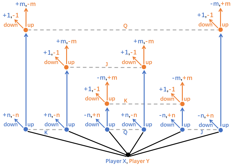
(a) The $(m,n)$-game

(b) The payoff matrix of the (2,1)-game: Treatment A

$(\textbf{m,n})\!=\!(2,1)$	$Y_{1}$	$Y_{2}$	$Y_{3}$	$Y_{4}$	$Y_{5}$	$Y_{6}$	$Y_{7}$	$Y_{8}$
$X_{1}$	0,  0	0,  0	0,  0	0,  0	0,  0	0,  0	0,  0	0,  0
$X_{2}$	0,  0	0,  0	1,  -1	1,  -1	1,  -1	1,  -1	2,  -2	2,  -2
$X_{3}$	2,  -2	-1,  1	2,  -2	-1,  1	3,  -3	0,  0	3,  -3	0,  0
$X_{4}$	2,  -2	-1,  1	3,  -3	0,  0	4,  -4	1,  -1	5,  -5	2,  -2
$X_{5}$	4,  -4	1,  -1	1,  -1	-2,  2	4,  -4	1,  -1	1,  -1	-2,  2
$X_{6}$	4,  -4	1,  -1	2,  -2	-1,  1	5,  -5	2,  -2	3,  -3	0,  0
$X_{7}$	6,  -6	0,  0	3,  -3	-3,  3	7,  -7	1,  -1	4,  -4	-2,  2
$X_{8}$	6,  -6	0,  0	4,  -4	-2,  2	8,  -8	2,  -2	6,  -6	0,  0

(c) The payoff matrix of the (3,2)-game: Treatment B

$(\textbf{m,n})\!=\!(3,2)$	$Y_{1}$	$Y_{2}$	$Y_{3}$	$Y_{4}$	$Y_{5}$	$Y_{6}$	$Y_{7}$	$Y_{8}$
$X_{1}$	0,  0	0,  0	0,  0	0,  0	0,  0	0,  0	0,  0	0,  0
$X_{2}$	-2,  2	-2,  2	0,  0	0,  0	0,  0	0,  0	2,  -2	2,  -2
$X_{3}$	2,  -2	-2,  2	2,  -2	-2,  2	4,  -4	0,  0	4,  -4	0,  0
$X_{4}$	0,  0	-4,  4	2,  -2	-2,  2	4,  -4	0,  0	6,  -6	2,  -2
$X_{5}$	6,  -6	2,  -2	2,  -2	-2,  2	6,  -6	2,  -2	2,  -2	-2,  2
$X_{6}$	4,  -4	0,  0	2,  -2	-2,  2	6,  -6	2,  -2	4,  -4	0,  0
$X_{7}$	8,  -8	0,  0	4,  -4	-4,  4	10,  -10	2,  -2	6,  -6	-2,  2
$X_{8}$	6,  -6	-2,  2	4,  -4	-4,  4	10,  -10	2,  -2	8,  -8	0,  0

(d) The payoff matrix of the (4,2)-game: Treatment C

$(\textbf{m,n})\!=\!(4,2)$	$Y_{1}$	$Y_{2}$	$Y_{3}$	$Y_{4}$	$Y_{5}$	$Y_{6}$	$Y_{7}$	$Y_{8}$
$X_{1}$	0,  0	*0,  0	0,  0	*0,  0	0,  0	0,  0	0,  0	0,  0
$X_{2}$	-2,  2	*-2,  2	1,  -1	1,  -1	1,  -1	1,  -1	4,  -4	4,  -4
$X_{3}$	2,  -2	-3,  3	2,  -2	-3,  3	5,  -5	0,  0	5,  -5	0,  0
$X_{4}$	0,  0	-5,  5	3,  -3	-2,  2	6,  -6	1,  -1	9,  -9	4,  -4
$X_{5}$	6,  -6	*1,  -1	1,  -1	-4,  4	6,  -6	1,  -1	1,  -1	-4,  4
$X_{6}$	4,  -4	-1,  1	2,  -2	-3,  3	7,  -7	2,  -2	5,  -5	0,  0
$X_{7}$	8,  -8	-2,  2	3,  -3	-7,  7	11,  -11	1,  -1	6,  -6	-4,  4
$X_{8}$	6,  -6	-4,  4	4,  -4	-6,  6	12,  -12	2,  -2	10, -10	0,  0

Figure 2: The parameterized (m,n) game. (a) The extensive form [3]. (b,c,d) The normal form of the game (the matrix elements are multiplied by 6).

The parameters are assigned as $(m,n)$ = (2, 1), (3, 2) and (4, 2), which are referred to as treatment A, B, and C, respectively. Details on the game design and the motivations are provided in SI – Game.

2.2 Classical game theory predictions

Method:

The concepts of static equilibrium and the iterated eliminating dominated strategy (IEDS) are useful when describing the full Nash-equilibrium-finding process, according to the classical game theory paradigm. For details of the method, see SI – Statics.

• For the three treatments, to solve the Nash equilibrium of the three bimatrix zero sum two person game, we can use quadratic programming method [20].

• For the three treatments, the order of the eliminating dominated strategies, as well as the surviving strategies, can be obtained by IEDS method.

Predictions:

The predictions and their verification methods are as follows:

• Distribution. The equilibrium distribution results are shown in figure 2a. Following the methods of conventional experimental research [4, 28, 6], the predictions can be verified using the data, denoted as $\rho^{E}$ and shown in Table A2.

• Cycle. IEDS provides the surviving strategy for a game, which is shown in Figure 3 and in the row titled ‘Surviving Strategy’ in Table 1. According to best-response analysis, the cycle’s existence and relative strength in each treatment (A, B, and C) can be predicted as (Yes, No, Yes), referring to Figure 3. These points can be verified using the experimental cycle ($\vartheta^{E}$) in section 3.2.

• Collapse. IEDS provides the eliminating order of a game. The results is shown in the row ’IEDS round’ in Table 1. Mathematical analysis of the best response analysis show that, among the dominated strategies, the strategy that is eliminated last could provide the pulse signal during the collapse. These points can be verified by the pulse ($\psi^{E}$) and the crossover points ($\chi^{E}$) using the experimental observations in section 3.3.

In additions, these three predictions can be applied to compare with those from dynamics theory. The results will be reported in section 3.4.

(a)

A	$Y_{2}$	$Y_{4}$
$X_{2}$	0,  0	1,  -1
$X_{6}$	1,  -1	-1,  1

(b)

B	$Y_{4}$
$X_{1}$	0,  0

(c)

C	$Y_{2}$	$Y_{4}$
$X_{1}$	0,  0	0,  0
$X_{2}$	-2,  2	1,  -1
$X_{5}$	1,  -1	-4,  4

Figure 3: The surviving strategy of the (A, B, C) game. The expected fixed patterns of the (A, B, C) game are a fixed orbital cycle, pure Nash equilibrium (a fixed point or signal star), and a mixed pattern, respectively.

Table 1: Equilibrium theory predictions and experiment protocol.

ID	Treatment ID	A		B		C
	Game-$(m,n)$	(2,1)		(3,2)		(4,2)
	Player ID	X	Y	X	Y	X	Y
Equili- brium Theory	IEDS Round 1	1,3,5,7	$\alpha^{*}$	3	$\alpha$	3	$\alpha$
	IEDS Round 2	4,8	-	2,4,6,7,8	-	4,6,7,8	-
	IEDS Round 3			-	2
	IEDS Round 4			5	-
	Survive	2,6	2,4	1	4	1,2,5	2,4
	strategy
Experi- ment Protocal	Session number	12		12		12
	Player in session	2		2		2
	Repeated round	1000		1000		1000
	Matching	Fix paired		Fix paired		Fix paired

${}^{*}\alpha$=1,3,5,6,7,8 means the strategies are eliminated simultaneously.

2.3 Game dynamics theory prediction

The game dynamics paradigm provides a set of concepts and methods on game evolution process [10, 8, 30, 17, 33]; This study adheres to this paradigm.

Method:

We utilize the logic dynamics equations system [26]; At the same time, referring to [6, 39, 17, 10], this study makes use of the noise parameter ($\lambda$ = 50) and the adjustment time step ($\triangle t$ = 0.02). Then, with random initial conditions, we can generate the time series of 1000 rounds data as long as the 1000 round experiment conducted in this research. Then, using the generated time series, we can calculate the predictions of the observations (distribution, cycle and collapse) simultaneously.

It is worth noting that, based on the experiences of previous studies [6, 39], we take the two parameters $(\lambda,\triangle t)$ simply by scanning two-dimensional parametric space, aiming for $\rho^{T}_{\textbf{Dyn}(\lambda,\triangle t)}$ to be approximately close to $\rho^{T}_{\textbf{QP}}$. We do not fix the two parameters by the experiment data.

Predictions:

Following the methods, the results are predictions that can be experimentally verified. These results are as follows:

• Distribution. The distribution of the treatments is shown in Figure 4(a) and Table A2 as $\rho^{T}_{\text{Dyn}}$, which is verifiable by the experiment.

• Cycle. The eigencycle spectra of the treatments are shown in Figure 4(b) as $\vartheta^{T}$. For further details about eigencycle spectra see Appendix A.3. The refined predictions are that, for treatments (A,B,C), there exist (strong, no, weak) cycles, respectively.

• Collapse. The theoretical accumulated curves ($\varrho^{T}$) are shown in Figure 4(c)-4(h). The numerical result of the crossover points are shown in Table A8. The statistically significant theoretical pulse signals are shown in Table A6. These predictions can be applied as the criterion to evaluate the consistency between the theory and the experiment.

  The crossover points ($\chi_{-}$) with crossover time $\tau>100$ are labelled with red arrows. According to the numerical results shown in Table A8, there are (4,0,2) $\chi_{-}$ red arrows in treatments (A,B,C).

2.4 Game experiment

The experiment was performed at Zhejiang University between August and September 2018. A total of 72 undergraduate students from Zhejiang University volunteered to serve as the human subjects of this experiment.

The main parameters and protocol are shown in the ’Experiment’ rows in Table 1. There were three treatments, and each was assigned 24 human subjects. The 24 subjects were divided into 12 sessions of 2 participants. The two players played a game with 1000 repeated in this fixed pairing. The reasoning behind the protocol design are explained in the Appendix—Experiment: Section 3.3.1 Design consideration).

In a session, a player can see observe sides strategy id ($X_{1},X_{2},...,X_{8}$) for player $X$ or ($Y_{1},Y_{2},...,Y_{8}$) for player $Y$. But a player can only observe her/his own realised payoffs and the strategy used of its own opponent. We do not provide the subject the payoff matrix, and no discussion allowed.

The experimental sessions lasted for an average of two hours. The payment of a subject, including CNY 20 for attending the session, as well as a payment based on the player’s rank, averaged CNY 120. The rank fee was determined by the rank of a participant’s total earning score in the 1000-round game, based on a comparison of players in the same role (player X or player Y) in the same experimental session. For details on the design, procedures and data, see SI—Experiment.

3 Results

In this section, we report the results of the experiment and the theoretical verification of the observations (distribution, cycle, and pulse), as well as the results of the model comparison.

3.1 Distribution

In order to illustrate the completeness and consistency, we report the distribution in brief. For the method and details relating to the data, see Appendix—A.3.

Measurement.

The strategy distribution and its convergence are reported. The convergence is measured according to the Euclidean distance $\delta$ from the experimental distribution $\rho^{E}$ in respect to two theoretical predictions (1) the static (Nash) equilibrium $\rho^{T}_{\text{S}}$, and (2) the time series produced by the dynamics model $\rho^{T}_{\text{D}}$.

Results.

For the experimental distribution ($\rho^{E}$) and its evolution, which is determined by the distribution values at various time intervals, as shown in Table A2, the main results are as follows:

1. As expected, for all (A,B,C) treatments, over time, the observed distribution ($\rho^{E}$) moves closer to the static equilibrium ($\rho^{T}_{\text{S}}$) and to the dynamics prediction ($\rho^{T}_{\text{D}}$). This is because the Euclidean distances decrease along time ($\triangle\delta_{\text{S}}<0$ and $\delta_{\text{D}}<0$) for all of the treatments, as shown in Table A3.

2. In all (A,B,C) treatments, the dynamics prediction $\rho^{T}_{\text{D}}$ performs better than the statics prediction $\rho^{T}_{\text{S}}$. This finding is supported by comparing the Euclidean distance during the last rounds, $\triangle\delta<0$, for all of the treatments, as shown in Table A3.

To summarize, for the distributions, the experimental observations are consistent with the theoretical predictions and with the existing literature [4, 23, 6, 5, 28, 17]. In other words, the full process shown in Figure 1(a) can be observed in our 1000 rounds of data.

3.2 Eigencycle

In order to illustrate illustrate the completeness and consistency, we report the cycle in brief.

Measurement

Referring to [34, 41, 40], we used the eigencycle spectrum $\vartheta^{E}$ to present the cycle in the experiments. We measured the eigencycle value of the 120 subspace of the game state space for each treatment, respectively; then normalise $\vartheta^{E}_{A},\vartheta^{E}_{B},\vartheta^{E}_{C}$ for treatments (A,B,C) to attain the maximum $|\vartheta^{E}|=1$. For more details on the measurements and the methods used for data presentation, see SI – Cycle.

Results

The experimental eigencycle spectrum $\vartheta^{E}$ is shown in Figure 5(b). The main results are as follows:

1. Observations on the (A,B,C) treatments, $\vartheta^{E}_{A},\vartheta^{E}_{B},\vartheta^{E}_{C}$ are consistent with the predictions made based on dynamics theory, $\vartheta^{T}_{A},\vartheta^{T}_{B},\vartheta^{T}_{C}$, respectively, as shown in Figure 4(b) and Figure 5(b). This is because the linear regression between $\vartheta^{E}$ and $\vartheta^{T}$ has $p<0.000$ for each treatment.

2. Our observations were consistent with the predictions made based on the statics theory. According to the eigencycle spectra for the three treatments, the cycle $(X_{2},X_{6})\times(Y_{2},Y_{4})$ in treatment A is the strongest. This consists the result of the best-response analysis, as shown in Figure 3. These finding are supported by the numerical analysis, as shown in Appendix A.3.1

In summary, the cycles observed in the experiment are consistent with the theoretical predictions. The consistency of the results is in keeping with the existing literature on cycles [34, 6, 31, 40, 41].

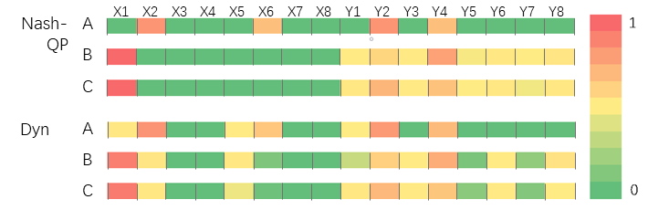
(a) Theoretical distributions ($\rho^{T}$)

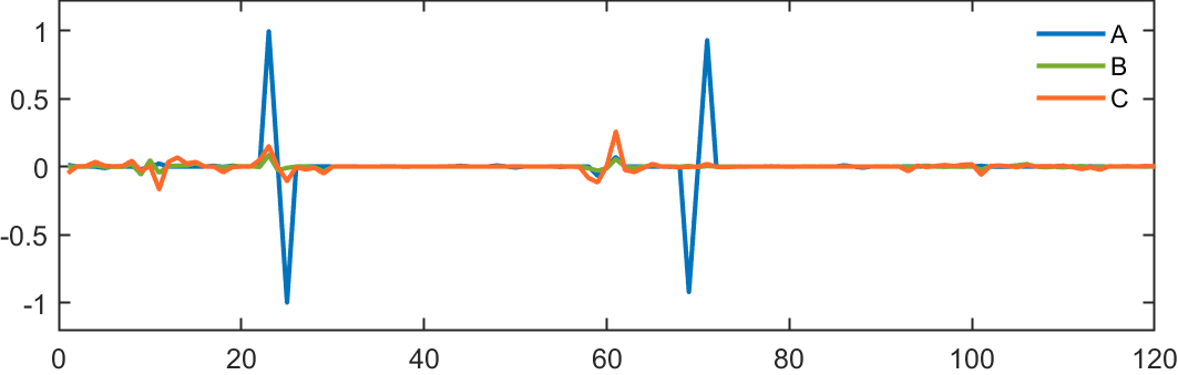
(b) Theoretical eigencycle spectrum ($\vartheta^{T}$)

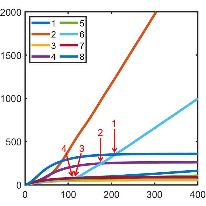
(c) $\varrho^{T}_{\text{(X-A)}}$

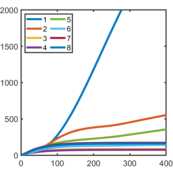
(d) $\varrho^{T}_{\text{(X-B)}}$

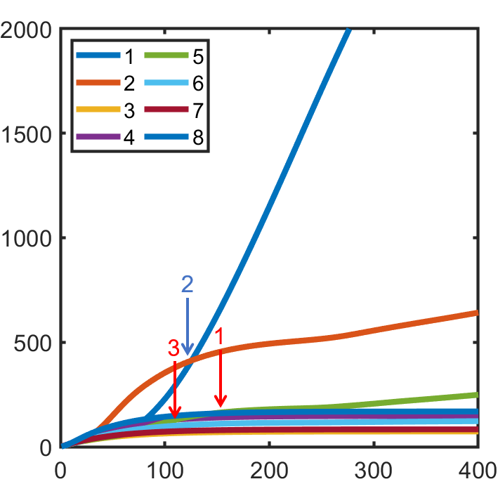
(e) $\varrho^{T}_{\text{(X-C)}}$

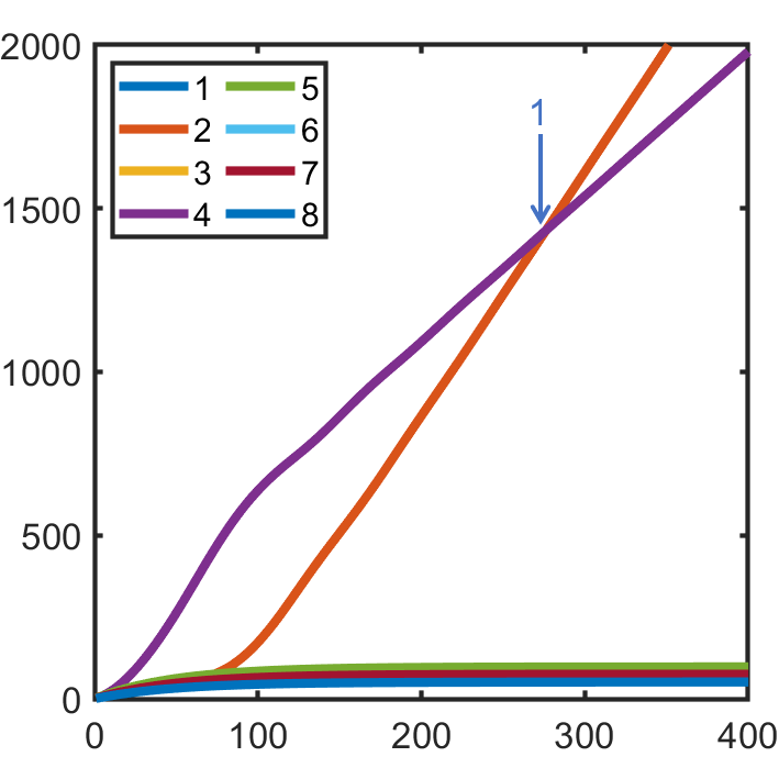
(f) $\varrho^{T}_{\text{(Y-A)}}$

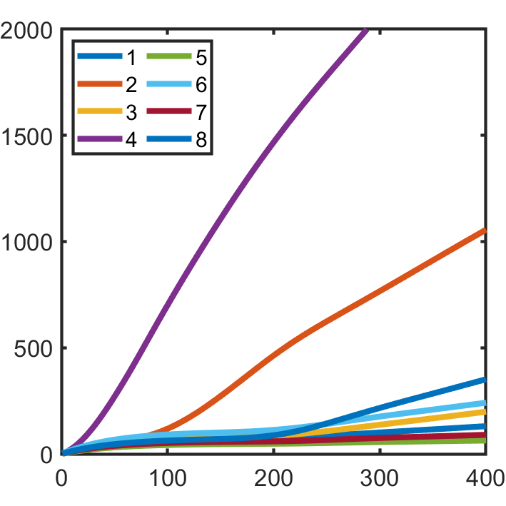
(g) $\varrho^{T}_{\text{(Y-B)}}$

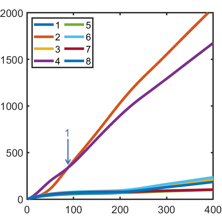
(h) $\varrho^{T}_{\text{(Y-C)}}$

Figure 4: Theoretical results of treatments A, B, and C. (a) Distributions $\rho^{T}$ from the two models; (b) eigencycle spectrum $\vartheta^{T}$; (c-h) accumulated curve ($\varrho^{T}$) of the player (X or Y). The crossover points ($\chi$) are labelled with arrows referring to the data in Table A8.

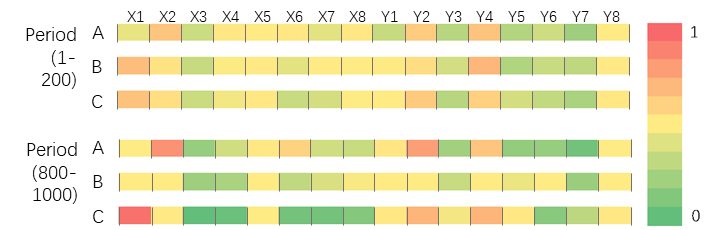
(a) Experimental distributions ($\rho^{E}$)

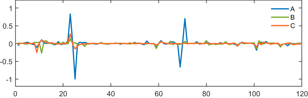
(b) Experimental eigencycle spectrum($\vartheta^{E}$)

(c) $\varrho^{E}_{\text{(X-A)}}$

(d) $\varrho^{E}_{\text{(X-B)}}$

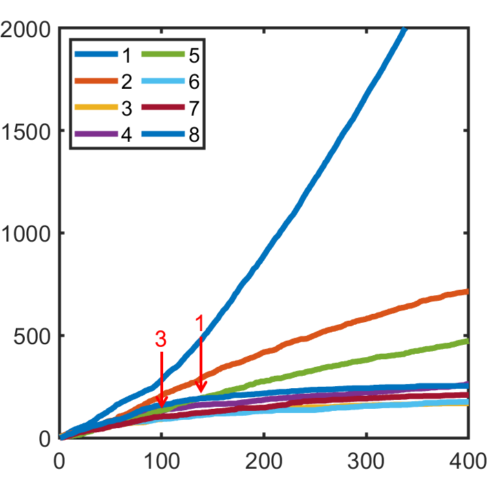
(e) $\varrho^{E}_{\text{(X-C)}}$

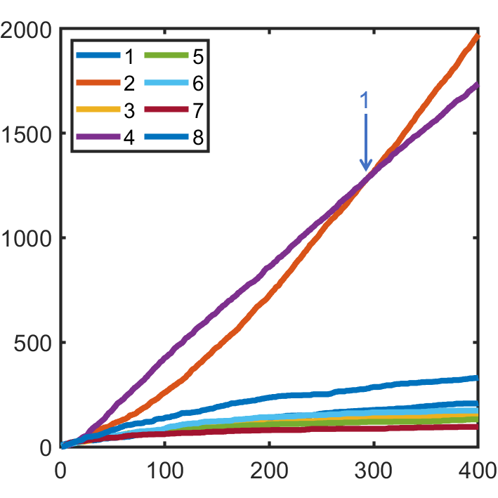
(f) $\varrho^{E}_{\text{(Y-A)}}$

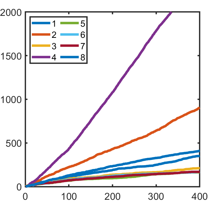
(g) $\varrho^{E}_{\text{(Y-B)}}$

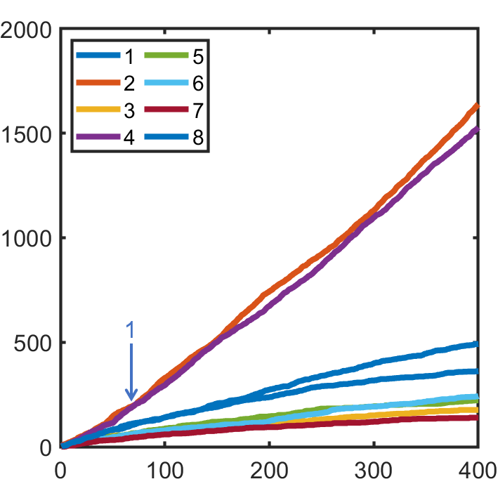
(h) $\varrho^{E}_{\text{(Y-C)}}$

Figure 5: Experiment results of treatments A, B, and C. (a)Average time of distribution for the 1-200 period and the 800-1000 period; (b) eigencycle spectrum $\vartheta^{E}$; (c-h) accumulated curve ($\varrho^{E}$) of the (X,Y) player over time. The crossover points ($\chi$) are labelled with arrows referring to the data in Table A7.

3.3 Collapse

The first research question requires us to identify the pulse in the collapse. To evaluate the consistency is to validate the dynamics paradigm during the collapse. Here, we offer the main results obtained regarding the collapse.

Measurement.

For the collapse, there are three relevant measurements – the accumulated curve ($\varrho$), the pulse signal ($\psi$) and the crossover points ($\chi$). For the definition of the measurements, see Appendix—A.4.1.

Results and explanation.

The main experimental results are as follows:

1. Accumulated curves ($\varrho^{E}$): The experimental accumulated curves $\varrho^{E}_{\text{j - i}}$ indicates the $i\in$(A,B,C) treatment and $j\in$ (X,Y) player, respectively, and there are six conditions. These are shown in Figure 5(c) - 5(h), which can be individually compared to the dynamics predictions $\varrho^{T}_{\text{j-i}}$, as shown in Figure 4(c) - 4(h). The results of the visual comparison support the consistency between the dynamics theory and the experimental results.

2. Crossover point ($\chi^{E}$): Following the dynamics prediction $\chi^{T}$ in Table A8, in the accumulated curve ($\varrho^{E}$), the $\chi^{E}_{-}$ are labelled using red arrows between $\textbf{D}^{-}/\textbf{D}^{+}$; meanwhile the $\chi^{E}_{+}$ are labelled using blue arrows between the $\textbf{D}^{+}/\textbf{D}^{+}$. These are shown in figure 5(c)-5(h). The consistency between theory and experiment is in visible.

3. The numerical results in Table A7 and Table A8 support the consistency between the theory and the experiment. For the dynamics predictions shown in Table A8, if $\tau^{T}\geq 89$ of $\psi([Y_{2},Y_{4}],\tau)$ is taken as the benchmark, there are have nine predicted samples. The experiment showed that, following the nine that were theoretically predicted, all eight of the $\chi^{E}$ labelled arrows in experiment have the largest $\tau$ values in terms of the related role (X,Y) and the treatment (A,B,C).

4. The crossover point is a consequence of the pulse in collapse. Referring to the relation between the pulse and the crossover time shown in section A.4.1, the observed crossover points are used to support the existence of pulse in [EO3.3.6] and [EO3.3.7].

5. Pulse signals ($\psi^{E}$): A pulse is a distinct observation made during the collapse. For the definition of a pulse, see Equation A13 in Appendix A.4.1. By examining the data, we observed pulses in significant. The main results regarding the pulses are as follows:

   • Existence of the pulse:

   • There are a total of nine pulses in significant ($p<0.05$), as shown in Table A5.

   • Among these nine pulses, three pulses are of the strongest statistical significance ($p<0.010$), as shown in Table 2.

   • The pattern of the pulses’ existence is consistent with the theoretical pattern:

   • The number of pulses in the treatments does not deviate the expectation by dynamics theory (see Table A6). More pulses are observed in treatment A than in B, and in B than in C.

   • All three of the pulses with the strongest significance ($p<0.010$) are included in category of the most expected pulses, according to dynamics theory (for details, see Table A6).

   • All four pulses with the strongest significance ($p\leq 0.011$) have the maximum surplus $\psi$ value among the nine pulse signals shown in Table A5.

   • The pattern of the pulses’ existence is consistent with the pattern of the crossover points.

   • Of the nine significant pulses ($p<0.05$), six are from treatment A and three are from C. More pluses are observed in treatment A than in C, as shown in Table A5. This is consistent with the $\chi^{E}$, in that there more significant crossover points observed in treatment A than in C, according to the $\chi^{E}_{-}$ with the red arrow in Table A7.

   • As predicted in Table A8, there are (4,0,2) red arrows in treatment (A,B,C), respectively. This is supported by the number of pulses and their significance in the experiment, as shown in Table A5.

   • On the other hand, there is no significant pulse signal ($p<0.05$) from the Y player in treatment A, B, or C. This is consistent with the dynamics predictions for pulses, as shown in Table A6.

   According to the pulse measurements, all of the significant results for pulses are consistent with the predictions made based on dynamics. No statistically significant evidence against the dynamics model was obtained.

   Treat-	Domin-	Domin-	Time	paired-	Surplus	Sample
   ments	ated	ation	block	ttest ($p$)		size
   	$s_{j}$	$s_{i}$	$[t_{0},t_{1}]$		$\psi$	N
   A	$X_{8}$	$X_{2}$	11-20	0.007	17	120
   A	$X_{8}$	$X_{6}$	11-20	0.002	19	120
   A	$X_{4}$	$X_{6}$	81-90	0.007	15	120

   Table 2: All of the observed pulses $\psi^{E}$ were highly significant ($p<0.010$). The symbols are explained in Equation A13 in Appendix A.4.1

The main result from the collapse in experiment is that, the significant pulse signals are observed, which supported by the observed crossover points. In addition to existed literature [33, 6, 5, 37, 17, 29, 2], in the collapse process, the consistency between the theory and the experiment empower by new empirical evidence.

3.4 Model comparison

Comparing the performances of the two theories under consideration is a key component of experiment research. Our main results are as follows:

1. In terms of distribution, the dynamics prediction ($\rho^{T}_{D}$) outperformed statics prediction ($\rho^{T}_{S}$). This is supported by data ($\rho^{E}$) in section 3.1.

2. For the cycle, the dynamics prediction outperformed the statics prediction. This is supported by comparing the results shown in EO2.1 and EO2.2 in section 3.2. Further analysis on cycle spectra can provide additional evidence to enhance the results, see section A.3.

3. For the collapse, dynamics theory can quantitatively predict the pulse ($\psi$) as well as the crossover point ($\chi^{E}$). The predictions made using IEDS, a component of statics theory in statics theory (TS3 in section 2.2), offer only limited explanation of the pulsing signals and the crossover point in terms of quantity. As a result, the dynamics model outperforms the statics.

In summary, game dynamics theory performs better than the static equilibrium theory, according to our data. This finding is consistent with the existed literature [6, 5, 17, 37, 33, 29, 2]. The summary of this section, see the first paragraph of the Discussion.

4 Discussion and conclusions

The main results of this study are the answers to the two key research questions posed above.

1. Regarding the first question, we observed that the pulse signal, which is a distinct observation of the collapse predicted using the dynamic model, is significant.

2. Regarding the second question, in the full process of finding equilibrium, we showed that all of the significant observations were those most clearly predicted by the dynamic model. The completeness and the consistency of the dynamics paradigm are supported by our data.

We posit that these results will assist the development of the game dynamics paradigm.

4.1 Implications

To explain the implications of our results, we can refer to the scientific paradigm of game dynamics theory [8, 9, 25, 18, 10, 26]. This paradigm has a self-reinforcing closed feedback workflow loop (for a brief introduction, see section A.5), which enhances its distinct set of concepts (e.g., natural selection, the evolutionary stable strategy, and, potentially, cycle [25, 10, 17, 6, 38, 37, 33, 29, 2]).

Since 1990 [8, 25],it has been expected that this paradigm would establish its own narrative of the game dynamics process, bringing about a paradigm shift with regard to the classical statics (Nash equilibrium) theory. However, the paradigm shift has not come to fruition. Those who are skeptical about using dynamics research to solve social and economic problems mainly focus on empirical observations [18, 25, 4].

Since 2010, the convenience of this method has been improved by empirical observations. The cycle is one example of this [7, 6, 40, 37, 39, 38, 32, 29, 2], and it may become a constitute element in the paradigm’s distinct set of concepts. Because a cycle generally exists in mixed-strategy Nash equilibrium behaviours, it is a consequence of the engagement of strategy interactions; moreover, it demonstrates game evolution, and is an exploitable PTDE.

We posit that the pulse in collapse can be constantly developed, similarly to the cycle, because of the following:

1. The pulse fulfils the experimental observation gap in the collapse, which is a legitimate constituent part of the full equilibrium-finding process (as shown in Figure 1).

2. The study on the pulse in collapse process can be helpful to the completeness and consistency of the game dynamics paradigm.

4.2 Related works

On the elimination of a dominated strategy

This study is not the unique to note the behaviours of the dominated strategy. For examples:

• Theoretically speaking, ‘A dominated strategy can dominate a domination before being dominated’; this phenomenon, namely, a pulse, is evident (e.g., in Gintis’ book [14], Figure 5.3, in section 5.8, the red mark during the infancy stage is the pulse signal). In finding the full Nash equilibrium process, the dominated strategies that are eliminated or survive have been extensively studied [16, 15, 21], but research on the pulse phenomenon is rare.

• In experimental terms, research into dominated strategies is not uncommon [24, 30, 27]. But these reports mainly focus on whether the dominated strategies are eliminated or attain equilibrium, but do not address what can be observed during the collapse.

The unique of this study in existed literature is that, it firstly provides the quantitative observation, in terms of the pulse, of the collapse process. By examining the collapse process, which has not been investigated before, the consistency and the completeness of the game dynamics paradigm are demonstrated.

Further research

Further research on the collapse and the pulse is needed. Although the existence of the pulse in the collapse has been explored and pulse experiment is consistent with the theory, it is far from being considered a legitimate constituent part of the paradigm.

The open question on how to select a dynamics model and its parameters when facing a real-life system is remained. In this study, following [1, 6, 39], we utilised logit dynamics, and fix its parameter grossly by the distribution closing to the equilibrium distribution by QR. Although we can capture all of the various observations in various treatments without changing the parameters, admittedly, this work can not answer the open question.

The collapse stage in games does not only move beyond the stationary concept of static equilibrium [28, 37],but also departs from the concept of non-equilibrium stationary states (e.g., cycle) [19, 39, 37]. By developing a better understanding of collapse, and of how to obtain the hierarchy of condensed structures or various dynamic equilibrium structures from a primordial soup or an existing state, we can expect solutions to appear in the coming decades.

Potential applications

Exploiting the PTDE can be profitable, e.g., in the arbitrage by high frequency trading (HFT) [36]. The arbitrage of HFT comes from predictable non-equilibrium in the short-term, rather than equilibrium in the long-term. The collapse is part of a process that is distant from equilibrium. It could therefore provide a helpful framework for understanding sudden shocks in a social system. During such periods, many unconventional strategy behaviors might appear to dominate. The findings related to the pulse support the statement: ’A dominated can dominate a domination before dominated’. This means that non-equilibrium behaviors can be profitable in the short term.

This study has real life applications in fields including artificial intelligence [22] and and the social systems addressed in [9, 25]. the collapse is a legitimate constituent part of the process of game evolution. The Nash equilibrium is not necessarily the best strategy during the infancy period when playing a complex game, e.g., Stratego [22].

Regarding general decision making in real-life social systems, philosophically, linear thinking may be harmful. In periods of turmoil, the power of myopia, or the power of the best response, must be properly acknowledged.

4.3 Conclusion

Based on a dynamic game with incomplete information, this investigation illustrates the full equilibrium finding process shown in figure 1, from random play to collapse to a fixed pattern (cycling and equilibrium). As a PTDE, the collapse constitutes fertile ground for the science of game dynamics, especially as it relates to the system of human social interactions.

Appendix A

A.1 Abbreviations

The abbreviations and mathematical symbols, shown in Table A1, are used in the main text, this appendix and the supplementary information.

PTDE		Predictable temporary deviation from equilibrium
N		Sample size for statistical analysis
$\text{Dyn}(\lambda,\Delta)$		Logit Dynamics with noise $\lambda$ and time step $\Delta$,
		a model in game dynamics theory
IEDS		Iterated eliminating dominated strategy,
		a method to find the Nash equilibrium
QP		Quadratic programming, an algorithm
		for Nash equilibrium distribution
$\textbf{D}^{\pm}$		$+$, domination strategy, survival strategy;
EO		Experimental observation
TS		Predictions from static equilibrium theory
TD		Predictions from dynamics theory
ET		Experiment data, used to compare the models’
Obs.		observations
SI		Supplementary information
$s_{i}$		The $i$-th optional strategy for a player
$\rho$		The proportion vector of strategies used
	$\rho(s_{i})$	The $i$-th component of $\rho$,
	$\rho(s_{i},t)$	The $\rho(s_{i})$ at time (round) $t$
	$\rho_{([t_{1},t_{2}])}$	The time average of $\rho$ between $[t_{1},t_{2}]$
	$\rho^{+}_{*}([s_{i},s_{j}])$	A surplus sample set
$\delta$		The Euclidean distance between two distribution
		vectors,used to evaluate their difference
$o$		A fixed point, rest point, or zero velocity point, equilibrium
$\lambda$		Eigenvalue
$\xi$		Eigenvector
$\eta_{i}$		The $i$-th component of a given eigenvector $\xi$
$\vartheta$		The eigencycle set in the 2D subspace set of a game
		space, describing the cyclic motion strength
	$\vartheta(m,n)$	The $\vartheta$ at dimension (1,2):=($\eta_{m},\eta_{n}$)
	$\vartheta(x)$	Eigencycle spectrum, where $x$ is a natural number
$\varrho$		Time-accumulated value curve of $\rho(t)$
	$\varrho(s_{i})$	the $\varrho$ of the $s_{i}$ strategy
$\psi$		A pulse signal
	$\psi([s_{i},s_{j}],[t_{1},t_{2}])$	A pulse signal of strategy $j$ over $i$
		during time interval $[t_{1},t_{2}]$
$\chi$		A crossover point, having two results $t$ and $\varrho$
	$\chi([s_{i},s_{j}],\tau)$	A crossover point of $\varrho(s_{i})$ and $\varrho(s_{j})$ at time
		$\tau$, and when $t=\tau-0^{+}$, $s_{j}>s_{i}$
	$\chi_{+}(s_{i},s_{j})$	$\chi$ if $s_{i}\in\textbf{D}^{+}\cap s_{j}\in\textbf{D}^{+}$
	$\chi_{-}(s_{i},s_{j})$	$\chi$ if $s_{i}\in\textbf{D}^{+}\cap s_{j}\in\textbf{D}^{-}$

Table A1: Abbreviations and mathematical symbols.

A.2 Distribution

This section reports the results on the distribution and its evolution, including the following elements:

• Theoretical and experimental numerical results of the average time distribution are shown Table A2.

• Numerical results relating to Euclidean distance, illustrating the evolution of the distribution, are shown in A3.

For more details of the measurements and data, see SI – Distribution.

Explanation of support [EO1] and [EO2].

In Table A3, the numerical Euclidean distance and its evolution are reported as follow:

1. The (1,2,4,5)-th row is the Euclidean distance of the given time interval.

2. The (3, 6)-th row is the difference in the Euclidean distance

   $$\triangle\delta_{\textbf{QP}}=\delta_{\textbf{QP[801,1000]}}-\delta_{\textbf{QP[1,200]}}<0$$ (A1)

   $$\triangle\delta_{\textbf{Dyn}}=\delta_{\textbf{Dyn[801,1000]}}-\delta_{\textbf{Dyn[1,200]}}<0$$ (A2)

   This means that $\rho^{E}$ is close to the predictions during the 1000 round game in all of the treatments (A,B,C).

3. The (7)-th row is the difference between the two models.

   $$\triangle\delta=\delta_{\textbf{Dyn[801,1000]}}-\delta_{\textbf{QP[801,1000]}}<0$$ (A3)

   This means that the $\rho^{E}_{800,1000}$ is closer to the expectation of the dynamics model than the Nash equilibrium according to the QP algorithm in all of the treatments (A,B,C).

[.5]0 Treatment	Period	id	$\rho^{E}_{(1,1000)}$		$\rho^{E}_{(1,500)}$		$\rho^{E}_{(500,1000)}$		$\rho^{E}_{(800,1000)}$		$\rho^{T}_{QP}$		$\rho^{T}_{Dyn(0.02,50)}$
[.5]0	Game		X	Y	X	Y	X	Y	X	Y	X	Y	X	Y
A	(2,1)	1	0.040	0.050	0.055	0.042	0.025	0.058	0.021	0.057	0.000	0.000	0.034	0.001
A	(2,1)	2	0.580	0.497	0.486	0.431	0.673	0.563	0.691	0.595	0.667	0.667	0.670	0.629
A	(2,1)	3	0.019	0.017	0.029	0.028	0.009	0.007	0.005	0.007	0.000	0.000	0.000	0.000
A	(2,1)	4	0.045	0.346	0.076	0.367	0.014	0.324	0.011	0.307	0.000	0.333	0.000	0.370
A	(2,1)	5	0.066	0.015	0.087	0.023	0.045	0.006	0.045	0.005	0.000	0.000	0.014	0.000
A	(2,1)	6	0.185	0.019	0.163	0.030	0.207	0.007	0.205	0.005	0.333	0.000	0.280	0.000
A	(2,1)	7	0.026	0.011	0.038	0.018	0.014	0.005	0.011	0.002	0.000	0.000	0.000	0.000
A	(2,1)	8	0.039	0.045	0.066	0.061	0.012	0.029	0.010	0.022	0.000	0.000	0.000	0.000
B	(3,2)	1	0.624	0.061	0.540	0.071	0.707	0.051	0.712	0.044	1.00	0.033	0.842	0.025
B	(3,2)	2	0.165	0.188	0.160	0.189	0.170	0.186	0.167	0.186	0.000	0.186	0.087	0.239
B	(3,2)	3	0.019	0.030	0.026	0.040	0.012	0.020	0.010	0.017	0.000	0.041	0.000	0.053
B	(3,2)	4	0.029	0.579	0.046	0.521	0.011	0.636	0.012	0.650	0.000	0.573	0.000	0.501
B	(3,2)	5	0.058	0.030	0.077	0.034	0.039	0.026	0.040	0.022	0.000	0.021	0.063	0.006
B	(3,2)	6	0.029	0.029	0.041	0.034	0.016	0.025	0.015	0.027	0.000	0.049	0.007	0.053
B	(3,2)	7	0.043	0.020	0.062	0.030	0.025	0.011	0.020	0.009	0.000	0.023	0.000	0.012
B	(3,2)	8	0.033	0.063	0.047	0.081	0.019	0.045	0.025	0.045	0.000	0.074	0.000	0.111
C	(4,2)	1	0.750	0.051	0.588	0.064	0.912	0.039	0.943	0.038	1.000	0.058	0.882	0.078
C	(4,2)	2	0.092	0.386	0.135	0.362	0.049	0.411	0.034	0.426	0.000	0.422	0.077	0.413
C	(4,2)	3	0.015	0.027	0.029	0.033	0.000	0.022	0.000	0.014	0.000	0.043	0.000	0.061
C	(4,2)	4	0.024	0.363	0.046	0.325	0.002	0.400	0.001	0.425	0.000	0.330	0.000	0.321
C	(4,2)	5	0.061	0.043	0.092	0.044	0.031	0.042	0.016	0.040	0.000	0.025	0.038	0.011
C	(4,2)	6	0.016	0.040	0.030	0.051	0.001	0.030	0.002	0.004	0.000	0.055	0.003	0.061
C	(4,2)	7	0.019	0.018	0.036	0.025	0.001	0.010	0.002	0.009	0.000	0.021	0.000	0.009
C	(4,2)	8	0.024	0.071	0.044	0.096	0.004	0.047	0.003	0.044	0.000	0.046	0.000	0.047

Table A2: Distribution. Columns 1-3 show the treatment, game parameter, and strategy, respectively. The blocks $\rho^{E}(t_{0},t_{1})$ are the experimental (X,Y) player’s time average of $\rho$ between $(t_{0},t_{1})$. $\rho^{T}_{QP}$ and $\rho^{T}_{Dyn(0.02,50)}$ are the prediction from statics and dynamics theory, respectively.

	Treatment
	A	B	C
$\delta_{\textbf{QP[1,200]}}$	0.4298	0.5551	0.5745
$\delta_{\textbf{QP[801,1000]}}$	0.3766	0.4047	0.4436
$\triangle\delta_{\textbf{QP}}$	$-$0.0532	$-$0.1504	$-$0.1309
$\delta_{\textbf{Dyn[1-200]}}$	0.0781	0.2088	0.1442
$\delta_{\textbf{Dyn[801-1000]}}$	0.0059	0.0097	0.0072
$\triangle\delta_{\textbf{Dyn}}$	$-$0.0722	$-$0.1991	$-$0.1370
$\triangle\delta$	$-$0.3707	$-$0.3950	$-$0.4364

Table A3: The Euclidean distance and its evolution. For details, ^′Explanation of support [EO1] and [EO2]^′.

A.3 Cycle

As the main focus of this study is the collapse, we report the cycle only briefly. The definition of the eigencycle spectrum, as well as the details of the numerical results of the eigencycle spectrum, are shown in SI – Cycle. This section includes the following contents:

1. Results on the maximum eigencycles in the eigencycle spectrum, in the experiment and in theory, respectively, are shown in Table A4.

2. The verification of the theories by experiment.

$$\begin{array}[]{|c|c|cc|r|}\hline\cr\addstackgap[.5]{\vphantom{0}}\text{Treatment}&x&m&n&\vartheta^{E}{}{}{}\\ \hline\cr\text{A}&25&2&12&-1.000\\ \text{A}&23&2&10&0.830\\ \text{A}&71&6&12&0.700\\ \text{A}&69&6&10&-0.660\\ \text{A}&101&10&12&-0.189\\ \text{A}&59&5&10&-0.110\\ \text{A}&9&1&10&-0.104\\ \text{A}&11&1&12&0.104\\ \text{A}&61&5&12&0.081\\ \text{A}&22&2&9&0.078\\ \text{A}&55&5&6&0.070\\ \text{A}&93&9&10&-0.067\\ \hline\cr\text{B}&11&1&12&-0.269\\ \text{B}&101&10&12&-0.148\\ \text{B}&59&5&10&-0.143\\ \text{B}&23&2&10&0.126\\ \text{B}&111&12&13&-0.098\\ \text{B}&80&7&12&0.081\\ \text{B}&29&2&16&-0.081\\ \text{B}&102&10&13&0.075\\ \text{B}&13&1&14&0.074\\ \text{B}&65&5&16&0.067\\ \text{B}&12&1&13&0.063\\ \text{B}&71&6&12&0.061\\ \hline\cr\text{C}&23&2&10&0.272\\ \text{C}&9&1&10&-0.257\\ \text{C}&25&2&12&-0.153\\ \text{C}&101&10&12&-0.094\\ \text{C}&11&1&12&0.086\\ \text{C}&93&9&10&-0.077\\ \text{C}&26&2&13&-0.066\\ \text{C}&12&1&13&0.066\\ \text{C}&61&5&12&0.056\\ \text{C}&111&12&13&-0.051\\ \text{C}&59&5&10&-0.045\\ \text{C}&104&10&15&0.044\\ \hline\cr\end{array}~{}~{}~{}~{}\begin{array}[]{|c|c|cc|r|}\hline\cr\addstackgap[.5]{\vphantom{0}}\text{Treatment}&x&m&n&\vartheta^{T}{}{}{}\\ \hline\cr\text{A}&25&2&12&-1.000\\ \text{A}&23&2&10&0.995\\ \text{A}&71&6&12&0.928\\ \text{A}&69&6&10&-0.923\\ \text{A}&61&5&12&0.068\\ \text{A}&59&5&10&-0.068\\ \text{A}&9&1&10&-0.021\\ \text{A}&11&1&12&0.021\\ \text{A}&1&1&2&0.011\\ \text{A}&5&1&6&-0.011\\ \text{A}&86&8&10&0.008\\ \text{A}&88&8&12&-0.008\\ \hline\cr\text{B}&23&2&10&0.084\\ \text{B}&9&1&10&-0.058\\ \text{B}&61&5&12&0.056\\ \text{B}&11&1&12&-0.046\\ \text{B}&10&1&11&0.044\\ \text{B}&29&2&16&-0.037\\ \text{B}&59&5&10&-0.030\\ \text{B}&24&2&11&-0.028\\ \text{B}&15&1&16&0.025\\ \text{B}&101&10&12&-0.024\\ \text{B}&106&11&12&0.018\\ \text{B}&8&1&9&0.017\\ \hline\cr\text{C}&61&5&12&0.256\\ \text{C}&11&1&12&-0.168\\ \text{C}&23&2&10&0.150\\ \text{C}&59&5&10&-0.117\\ \text{C}&25&2&12&-0.107\\ \text{C}&58&5&9&-0.084\\ \text{C}&13&1&14&0.067\\ \text{C}&101&10&12&-0.060\\ \text{C}&29&2&16&-0.051\\ \text{C}&1&1&2&-0.049\\ \text{C}&22&2&9&0.048\\ \text{C}&8&1&9&0.042\\ \hline\cr\end{array}$$

Table A4: Experimental cycle $\vartheta^{E}$ and the theoretical cycle $\vartheta^{T}$. The top 12 maximum strengths in the eigencycles of the spectrum from treatments (A,B,C). $x$ is the $x$-axis value in the eigencycle spectrum, and ($m,n$) are the strategy IDs in the unified dimension of the game, which are defined in SI—Cycle.

A.3.1 Verify the statics

In the main text section 2.2 [TS2], we state that the cycle’s existence in treatment-(A, B, C) can be predicted as (Yes, No, Yes), respectively. This prediction is based on the IEDS approach in the static equilibrium theory.

From Table A4, we obtain the following results.

• In treatment A, the closed loops are

  $$2\rightarrow 10\rightarrow 6\rightarrow 12\rightarrow 2$$ (A4)

• In treatment C, the closed loops are

  $$2\rightarrow 10\rightarrow 5\rightarrow 12\rightarrow 2$$ (A5)

  $$2\rightarrow 10\rightarrow 1\rightarrow 12\rightarrow 2$$ (A6)

the IEDS predictions for the cycle are supported. We observed a weak cycle in treatment B, which is not regarded as evidence against IDES because of its weakness, referring to equation A7.

A.3.2 Verification of the dynamics theory

The predictions given in the main text section 2.3 [TD2] are verified here. In treatments A and C, the predictions match the experimental data:

• In the cycle loop, there exist cycles for equation A4 in treatment A, and for equation A5 and A6 in treatment C;

• For the strength of the cycle loop, referring to Table A4, comparing the average of the strength of $\vartheta^{E}_{\text{Treatment}}$ in the loops, the result is

  $$\vartheta^{E}_{\text{A}}>\vartheta^{E}_{\text{C}}>\vartheta^{E}_{\text{B}.}$$ (A7)

For treatment B, the dynamics predicts little cycle. Considering equation A7, we do not regard the loop of $\vartheta_{B}^{E}$ as significant evidence against the prediction. As result, the consistency between the dynamics and the experiment is supported.

A.4 Collapse

This section includes the measurement definition for collapse, as well as the experimental data. For more details on this subsection, see SI – Collapse.

A.4.1 Measurement definition

Conceptual Example

Figure A1 offers an example of the pulse signal, accumulated curve and the crossover points. It is derived from the theoretical results of the strategy evolution over time of the X population in treatment A.

Figure A1: Conceptual figure for the pulse signal and the crossover point during a space collapse process. (a) Illustrates a pulse of strategy 8 in the strategy proportion time series $\rho(x_{8},t)$, which dominates when $t\in[0,30]$ and is eliminated (at $t\approx 130$). (b) Illustrates a crossover point $\chi([x_{2},x_{8}],70)$ (see the red arrows) in the accumulated curves $\varrho(x_{2},t)$ and $\varrho(x_{8},t)$.

Accumulated curve ($\varrho$)

We denote the accumulated $s_{k}$ strategy used in the time interval $[t_{0},t_{1}]$, which is: $\varrho(x_{k},t)$, which is

$$\varrho(s_{k},t_{0},t_{1})=\int_{t_{0}}^{t_{1}}\rho(s_{k},t)dt,$$ (A8)

where $\rho(x_{k},t)$ is the proportion of the observed $s_{k}$ at time $t$. In this study, we ake use of discrete time version and set $dt=1$. Without additional specification, in this study we set $t_{0}=0$, and the discrete version of the Equation A8 can be rewrites as

$$\varrho(s_{k},t)=\sum_{t^{\prime}=0}^{t}\rho(s_{k},t^{\prime}),$$ (A9)

which is the accumulated curve in this study.

Pulse signal

A pulse signal, or pulse, can be defined following these steps:

1. A sample of surplus in time series, denoted as $\rho^{+}\big{(}[s_{i},s_{j}],t\big{)}$, is the proportion difference between two strategies $[s_{i},s_{j}]$ at $t$,

   $$\rho^{+}\big{(}[s_{i},s_{j}],t\big{)}=\rho(s_{j},t)-\rho(s_{i},t).$$ (A10)

2. A surplus sample set $\rho^{+}_{*}$ refers to the surplus samples from a given successive time interval $[t_{0},t_{1}]$ (time block),

   $$\rho^{+}_{*}\big{(}[s_{i},s_{j}],[t_{0},t_{1}]\big{)}=\{\rho^{+}\big{(}[s_{i},s_{j}],t_{k}\big{)},~{}\forall t_{k}\in[t_{0}\!\!+\!\!1,t_{0}\!\!+\!\!2,...,t_{1}]\}.$$ (A11)

3. Sample size N. For statics analysis, the sample set size is

   $$\textbf{N}=(t_{1}-t_{0})\times\text{Number of experiment session}$$ (A12)

   For example, assuming that a time block is set as 10 rounds, from the 81${}^{s}t$ round to 90${}^{t}h$ round in a 1000 round repeated game session, the element of the set is 10. We have 12 sessions for a given treatment, so the sample size N is 120.

4. Pulse ($\psi$) is the total surplus of $s_{j}$ over $s_{i}$ in a time block $[t_{0},t_{1}]$:

   $$\psi\big{(}[s_{i},s_{j}],[t_{0},t_{1}]\big{)}=\sum_{t_{k}=t_{0}+1}^{t_{1}}\rho^{+}\big{(}[s_{i},s_{j}],t_{k}\big{)};$$ (A13)

   For example, in the top line in Table A5, the $\psi=17$. The explanation for this is that:

   • $X_{8}\in\textbf{D}^{-}$ is a dominated, and $X_{2}\in\textbf{D}^{+}$ is a domination.

   • There are 120 samples from the X population of treatment A and in the $t\in[11-20]$ rounds of the $\text{ses}\in[1,12]$ sessions.

   • The surplus observed is the sum over the sample set shown in equation A11. That is

     $$\sum_{\text{ses}=1}^{12}\sum_{t=11}^{20}\big{(}\rho(X_{8},t,\text{ses})-\rho(X_{2},t,\text{ses})\big{)}=17$$ (A14)

5. The statistical significance of a pulse $\psi$ is reported by the ttest over the surplus sample set $\rho^{+}_{*}$ shown in Equation A11. On the sample size N for ttest, see the example following the Equation A12.

6. Strong significant When $p<0.010$, the statistic result is reported to be ‘in strongly significant’. When $0.010\leq p<0.050$, the statistic result is reported as ‘in significant‘ but not as ‘in strongly significant‘.

Crossover point: $\chi(x_{i},x_{j},\tau)$

The definition of the crossover point depends on the accumulated curve ($\varrho$) shown in Equation A9. Assuming that:

$$\varrho(s_{i},t)-\varrho(s_{j},t)=0$$ (A15)

the crossover point is defined as $\chi(s_{i},s_{j},\tau)$ in which

• $\tau$ is the solution of the $t$

• $\chi(s_{i},s_{j},\tau)$ := $\varrho(s_{i},t)=\varrho(s_{j},t)$

The two classes of crossover points

• $\chi_{+}$ — when the paired comparison is between two ($\textbf{D}^{+}$), for example, the blue arrows in Figure 5(c) - 5(h) are the crossover points $\chi_{+}$.

• $\chi_{-}$ — when the paired comparison is between the ($\textbf{D}^{-}$) and ($\textbf{D}^{+}$), for example, the red arrows in Figure 5(c) - 5(h) are the crossover points $\chi_{-}$.

The relation between the pulse and the crossover time.

Based on the results reported in [E32.6] in section 3.3, we hypothesize that, if a crossover $\chi_{-}([x_{i},x_{j}],\tau)$ ( $s_{j}\in\textbf{D}^{-}$ and $s_{i}\in\textbf{D}^{+}$) has larger $\tau$, $s_{j}$ is more strongly expected to provide the pulse signal.

Assuming that $\rho(s_{i})$ and $\rho(s_{j})$ are equal at $t=0$, if a long run dominated ($s_{j}\in\textbf{D}^{-}$) has a pulse signal referring to a long run domination ($s_{i}\in\textbf{D}^{+}$), that is

$$\rho(x_{j},t)>\rho(x_{i},t)~{}~{}~{}~{}~{}~{}\forall t\in[0,T],$$ (A16)

As a mathematical result, there must be a crossover point in its accumulated curve $\varrho(x_{j},\tau)$ referring to $\varrho(x_{i},\tau)$ in which $\tau>T$. This is one explanation for the hypothesis.

For example, in experimental pulse $\psi^{E}$ (Table 2), all the strongest significant pulses belong to the largest $\tau$ in $\chi^{E}$ (Table A7). The result reported in [E32.6] refers to this mathematical property.

A.4.2 Data

Here, we present the data that support the results shown in section 3.3 in main text.

1. 1. The experimental pulse signal observed is statistically significant (p¡0.05): see Table A5

2. The theoretical pulse signal in statistical significant; Listed are the top 10 samples ordered by the time block surplus values of treatments (A,B,C): see Table A6. Note: the time series from the dynamics model are smooth, meaning that more significant pulse signals can be obtained from this model, when compared with those from the highly stochastic human subject experimental time series..

3. Experimental crossover point: see Table A7

4. Theoretical crossover point: see Table A8

Treat-	Domin-	Domin-	time	paired-	Surplus	Sample
ments	ated	ation	block	ttest($p$)		size
	$s_{j}$	$s_{i}$	$[t_{0},t_{1}]$		$\psi^{E}$	N
A	$X_{8}$	$X_{2}$	11-20	0.007	17	120
A	$X_{8}$	$X_{6}$	11-20	0.002	19	120
A	$X_{8}$	$X_{2}$	21-30	0.011	15	120
A	$X_{4}$	$X_{6}$	41-50	0.027	13	120
A	$X_{1}$	$X_{6}$	81-90	0.023	12	120
A	$X_{4}$	$X_{6}$	81-90	0.007	15	120
C	$X_{8}$	$X_{5}$	1-10	0.027	11	120
C	$X_{7}$	$X_{5}$	11-20	0.049	10	120
C	$X_{8}$	$X_{5}$	11-20	0.049	10	120

Table A5: Statistically significant experimental pulses ($\psi^{E}$) ($p$¡0.05).

Treat-	Domin-	Domin-	time	paired-	Surplus	Sample
ments	ated	ation	block	ttest($p$)		size
	$s_{j}$	$s_{i}$	$[t_{0},t_{1}]$		$\psi^{T}$	N
A	$X_{8}$	$X_{6}$	21-31	0.000	35.04	120
A	$X_{8}$	$X_{2}$	21-31	0.000	34.75	120
A	$X_{8}$	$X_{6}$	31-41	0.000	29.97	120
A	$X_{8}$	$X_{2}$	11-21	0.000	29.20	120
A	$X_{8}$	$X_{6}$	11-21	0.000	29.08	120
A	$X_{8}$	$X_{6}$	41-51	0.000	24.47	120
A	$X_{4}$	$X_{6}$	41-51	0.000	23.87	120
A	$X_{8}$	$X_{2}$	31-41	0.000	23.84	120
A	$X_{4}$	$X_{6}$	51-61	0.000	22.01	120
A	$X_{4}$	$X_{6}$	31-41	0.000	20.47	120
A	$X_{8}$	$X_{6}$	51-61	0.000	19.98	120
A	$X_{4}$	$X_{6}$	61-71	0.000	18.84	120
B	$X_{7}$	$X_{1}$	21-31	0.000	18.05	120
C	$X_{8}$	$X_{5}$	11-21	0.000	21.64	120
C	$X_{8}$	$X_{1}$	11-21	0.000	21.64	120
C	$X_{8}$	$X_{2}$	11-21	0.000	18.75	120
C	$X_{8}$	$X_{5}$	21-31	0.000	18.39	120
C	$X_{8}$	$X_{1}$	21-31	0.000	18.39	120

Table A6: Theoretical pulse ($\psi^{T}$). The most strongly expected top 18 samples (twice the $\psi^{E}$ is significant) ordered by the $\psi^{T}$ values of all the treatments (A,B,C). Note: the time series from the dynamics model are smooth, meaning that more significant pulse signals can be obtained from this model, when compared with those from the highly stochastic experimental time series.

Treat-	Domin-	Domin-	Crossover	Arrow
[.5]0 ment	ation	ated	Time ($\tau$)	Color	ID	Fig ID
$A$	$X_{2}$	$X_{1}$	47	-	-	Fig 5(c)
$A$	$X_{2}$	$X_{6}$	47	-	-
$A$	$X_{2}$	$X_{7}$	52	-	-
$A$	$X_{2}$	$X_{3}$	55	-	-
$A$	$X_{2}$	$X_{4}$	58	-	-
$A$	$X_{2}$	$X_{5}$	58	-	-
$A$	$X_{2}$	$X_{8}$	67	-	-
$A$	$X_{6}$	$X_{1}$	44	-	-
$A$	$X_{6}$	$X_{3}$	74	-	-
$A$	$X_{6}$	$X_{3}$	79	-	-
$A$	$X_{6}$	$X_{7}$	92	red	4
$A$	$X_{6}$	$X_{1}$	106	red	3
$A$	$X_{6}$	$X_{5}$	139	-	-
$A$	$X_{6}$	$X_{4}$	169	red	2
$A$	$X_{6}$	$X_{8}$	186	red	1
$A$	$Y_{2}$	$Y_{4}$	297	blue	1	Fig 5(f)
$C$	$X_{2}$	$X_{8}$	45	-	-	Fig 5(e)
$C$	$X_{5}$	$X_{6}$	49	-	-
$C$	$X_{5}$	$X_{6}$	54	-	-
$C$	$X_{5}$	$X_{3}$	56	-	-
$C$	$X_{5}$	$X_{4}$	100	red	3
$C$	$X_{5}$	$X_{8}$	138	red	1
$C$	$Y_{2}$	$Y_{4}$	74	blue	1	Fig 5(h)

Table A7: Experimental crossover point $\chi^{E}$ at $\tau^{E}>40$. The arrow columns refer to the arrows in Figure 5(c)-5(h), based on the theoretical arrows in Table A8. For the definition of $\tau$, see Equation A15.

Treat-	Domin-	Domin-	Crossover	Arrow
[.5]0 ment	ation	ated	Time ($\tau$)	Color	ID	Fig ID
$A$	$X_{2}$	$X_{4}$	62	-	-	Fig 4(c)
$A$	$X_{2}$	$X_{8}$	86	-	-
$A$	$X_{6}$	$X_{5}$	65	-	-
$A$	$X_{6}$	$X_{7}$	116	red	4
$A$	$X_{6}$	$X_{1}$	117	red	3
$A$	$X_{6}$	$X_{4}$	177	red	2
$A$	$X_{6}$	$X_{8}$	209	red	1
$A$	$Y_{2}$	$Y_{1}$	71	-	-	Fig 4(f)
$A$	$Y_{2}$	$Y_{5}$	74	-	-
$A$	$Y_{2}$	$Y_{4}$	277	blue	1
$B$	$X_{1}$	$X_{3}$	42	-	-
$B$	$X_{1}$	$X_{6}$	56	-	-
$B$	$X_{1}$	$X_{8}$	69	-	-
$B$	$X_{1}$	$X_{7}$	72	-	-
$B$	$X_{1}$	$X_{5}$	75	-	-
$B$	$X_{1}$	$X_{2}$	84	-	-
$C$	$X_{1}$	$X_{7}$	52	-	-	Fig 4(e)
$C$	$X_{1}$	$X_{6}$	66	-	-
$C$	$X_{1}$	$X_{4}$	77	-	-
$C$	$X_{1}$	$X_{8}$	82	-	-
$C$	$X_{1}$	$X_{2}$	126	blue	2
$C$	$X_{5}$	$X_{7}$	61	-	-
$C$	$X_{5}$	$X_{6}$	82	-	-
$C$	$X_{5}$	$X_{4}$	112	red	3
$C$	$X_{5}$	$X_{8}$	144	red	1
$C$	$Y_{2}$	$Y_{4}$	89	blue	1	Fig 4(h)

Table A8: Theoretical crossover point $\chi^{T}$ at $\tau^{T}>40$. The arrow columns relate to the arrows ($\tau>89$) in Figure 4(c)-4(h). For the definition of $\tau$, see Equation A15.

A.5 The game dynamics paradigm and its workflow

Similarly to the paradigms found in natural science, the game dynamics paradigm is also a distinct set of concepts, including theories, research methods, postulates, and standards for what constitutes legitimate contributions to a field. The reality and accuracy, as well as the completeness and consistency, of this distinct set of concepts must be proven. Key to developing a paradigm is a closed-loop of workflow. The workflow includes the following steps:

1. Describe a game (G) and its playing protocol (P);

2. Take a proper dynamics equation system T (e.g., replicator dynamics or logit dynamics) and specify the parameters of T by (G,P). Then, derive the theoretical observation O^T(G,P) by solving T(G,P), e.g., the reset point, the eigen system, or by time series analysis among others technologies;

3. Conduct experiments or collect empirical data to measure the observation O^E(G,P)

4. Evaluate the O^T(G,P) by empirical observation O^E(G,P).

5. Iterate Step 1 to Step 4 and feedback to step 1 as a loop, by trial and error, to find the best fit between the theory and the empirical system in general.

This iterated closed-loop workflow is widely applied in various scientific fields, and can constantly improve the establishment of a paradigm. In addition to the reality and the accuracy, the paradigm is endorsed by the completeness and the consistency between:

$$O^{T}(P,G)~{}~{}\text{vs}~{}~{}O^{E}(P,G)$$

endorse the paradigm. Social science follows this workflow, as does natural science[10, 4, 23].

References

- [1] Raymond Battalio, Larry Samuelson, and John Van Huyck. Optimization incentives and coordination failure in laboratory stag hunt games. Econometrica, 69(3):749–764, 2001.
- [2] Volker Benndorf, Ismael Martínez-Martínez, and Hans-Theo Normann. Games with coupled populations: An experiment in continuous time. Journal of Economic Theory, 195:105281, 2021.
- [3] Ken Binmore. Game theory: a very short introduction, volume 173. Oxford University Press, 2007.
- [4] Colin F Camerer. Behavioral game theory: Experiments in strategic interaction. Princeton University Press, 2003.
- [5] Timothy N Cason, Daniel Friedman, and Ed Hopkins. Testing the TASP: An experimental investigation of learning in games with unstable equilibria. Journal of Economic Theory, 145(6):2309–2331, 2010.
- [6] Timothy N Cason, Daniel Friedman, and Ed Hopkins. Cycles and instability in a rock–paper–scissors population game: a continuous time experiment. Review of Economic Studies, 81(1):112–136, 2014.
- [7] Timothy N Cason, Daniel Friedman, and Ed Hopkins. An experimental investigation of price dispersion and cycles. Journal of Political Economy, 129(3):789–841, 2021.
- [8] Daniel Friedman. Evolutionary games in economics. Econometrica: Journal of the Econometric Society, pages 637–666, 1991.
- [9] Daniel Friedman. Evolutionary economics goes mainstream: A review of the theory of learning in games. Journal of Evolutionary Economics, 8(4):423–432, 1998.
- [10] Daniel Friedman and Barry Sinervo. Evolutionary games in natural, social, and virtual worlds. Oxford University Press, 2016.
- [11] Emerging Technology from the arXiv. Best of 2014: How to win at rock-paper-scissors — MIT technology review, 2014. [Online; accessed 07-January-2023].
- [12] Drew Fudenberg and David K Levine. The theory of learning in games, volume 2. MIT press, 1998.
- [13] Drew Fudenberg and David K Levine. Whither game theory? towards a theory of learning in games. Journal of Economic Perspectives, 30(4):151–70, 2016.
- [14] Herbert Gintis et al. Game theory evolving: A problem-centered introduction to modeling strategic behavior. Princeton university press, 2000.
- [15] Josef Hofbauer and William H. Sandholm. Survival of dominated strategies under evolutionary dynamics. Theoretical Economics, 6(3):341–377, 2011.
- [16] Josef Hofbauer and Jörgen W. Weibull. Evolutionary selection against dominated strategies. JEL, 71(2):558–573, 1996.
- [17] Moshe Hoffman, Sigrid Suetens, Uri Gneezy, and Martin A Nowak. An experimental investigation of evolutionary dynamics in the rock-paper-scissors game. Scientific reports, 5(1):1–7, 2015.
- [18] Michihiro Kandori. Adjustment dynamics for human players. Nobel Symposium on One Hundred Years of Game Theory, December 17–19, 2021.
- [19] Melvin Lax. Fluctuations from the nonequilibrium steady state. Reviews of modern physics, 32(1):25, 1960.
- [20] Olvi L Mangasarian and H Stone. Two-person nonzero-sum games and quadratic programming. Journal of Mathematical Analysis and applications, 9(3):348–355, 1964.
- [21] Panayotis Mertikopoulos and William H Sandholm. Learning in games via reinforcement and regularization. Mathematics of Operations Research, 41(4):1297–1324, 2016.
- [22] Julien Perolat et al. Mastering the game of stratego with model-free multiagent reinforcement learning. Science, 378(6623):990–996, 2022.
- [23] Charles R Plott and Vernon L Smith. Handbook of experimental economics results, volume 1. Elsevier, 2008.
- [24] Amnon Rapoport and Wilfred Amaldoss. Mixed strategies and iterative elimination of strongly dominated strategies: An experimental investigation of states of knowledge. Journal of Economic Behavior & Organization, 42(4):483–521, 2000.
- [25] Larry Samuelson. Game theory in economics and beyond. Journal of Economic Perspectives, 30(4):107–30, 2016.
- [26] William H Sandholm. Population games and evolutionary dynamics. MIT press, 2010.
- [27] Rene Saran. Bounded depths of rationality and implementation with complete information. Journal of Economic Theory, 165:517–564, 2016.
- [28] Reinhard Selten and Thorsten Chmura. Stationary concepts for experimental 2x2-games. American Economic Review, 98(3):938–66, 2008.
- [29] Daniel Stephenson. Coordination and evolutionary dynamics: When are evolutionary models reliable? Games and Economic Behavior, 113:381–395, 2019.
- [30] John Van Huyck, Frederick Rankin, and Raymond Battalio. What does it take to eliminate the use of a strategy strictly dominated by a mixture? Experimental economics, 2(2):129–150, 1999.
- [31] Yijia Wang, Xiaojie Chen, and Zhijian Wang. Testability of evolutionary game dynamics based on experimental economics data. Physica A: Statistical Mechanics and its Applications, 486:455–464, 2017.
- [32] Zhijian Wang and Bin Xu. Evolutionary rotation in switching incentive zero-sum games. arXiv:1203.2591, 2012.
- [33] Zhijian Wang, Bin Xu, and Hai-Jun Zhou. Social cycling and conditional responses in the rock-paper-scissors game. Scientific reports, 4:5830, 2014.
- [34] Zhijian Wang, Shujie Zhou, Qinmei Yao, and Yijia Wang. Dynamic structure in four-strategy game: Theory and experiment. Contributions to Game Theory and Management, page accepted, 2022.
- [35] Wikipedia. Gravitational collapse — Wikipedia, the free encyclopedia, 2023. [Online; accessed 07-January-2023].
- [36] Wikipedia. High frequency trading — Wikipedia, the free encyclopedia, 2023. [Online; accessed 07-January-2023].
- [37] Bin Xu, Shuang Wang, and Zhijian Wang. Periodic frequencies of the cycles in 2 2 games: evidence from experimental economics. The European Physical Journal B, 87(2):46, 2014.
- [38] Bin Xu and Zhijian Wang. Evolutionary dynamical pattern of ’coyness and philandering’: Evidence from experimental economics. Unifying Themes in Complex Systems, 8, 2011.
- [39] Bin Xu, Hai-Jun Zhou, and Zhijian Wang. Cycle frequency in standard rock–paper–scissors games: evidence from experimental economics. Physica A: Statistical Mechanics and its Applications, 392(20):4997–5005, 2013.
- [40] Qinmei Yao. Theoretical analysis and experiment of dynamic structure of high dimensional game. https://cdmd.cnki.com.cn/Article/CDMD-10335-1021626407.htm,doi=10.27461/d.cnki.gzjdx.2021.000847, 2021.
- [41] Wang Zhijian and Yao Qingmei. Human social cycling spectrum. arXiv preprint arXiv:2012.03315, 2020.