Differential Aggregation against General Colluding Attackers

Abstract

Local Differential Privacy (LDP) is now widely adopted in large-scale systems to collect and analyze sensitive data while preserving users’ privacy. However, almost all LDP protocols rely on a semi-trust model where users are curious-but-honest, which rarely holds in real-world scenarios. Recent works  [65, 12, 7] show poor estimation accuracy of many LDP protocols under malicious threat models. Although a few works have proposed some countermeasures to address these attacks, they all require prior knowledge of either the attacking pattern or the poison value distribution, which is impractical as they can be easily evaded by the attackers.

In this paper, we adopt a general opportunistic-and-colluding threat model and propose a multi-group Differential Aggregation Protocol (DAP) to improve the accuracy of mean estimation under LDP. Different from all existing works that detect poison values on individual basis, DAP mitigates the overall impact of poison values on the estimated mean. It relies on a new probing mechanism EMF (i.e., Expectation-Maximization Filter) to estimate features of the attackers. In addition to EMF, DAP also consists of two EMF post-processing procedures (EMF* and CEMF*), and a group-wise mean aggregation scheme to optimize the final estimated mean to achieve the smallest variance. Extensive experimental results on both synthetic and real-world datasets demonstrate the superior performance of DAP over state-of-the-art solutions.

I Introduction

In the era of big data, privacy-preserving technologies are essential to collect sensitive data and analyse their statistical features (e.g., frequency and mean) while preserving individual’s data privacy. Among them, local differential privacy (LDP) is widely deployed for distributed data collection in large-scale systems (e.g., Chrome and iOS). In an LDP protocol, users only provide perturbed data to collectors, who then estimate some statistics, e.g., mean and frequency estimation, the two most fundamental ones  [1, 4, 14, 64, 39, 20, 62, 66, 47], from these data. A fundamental assumption of LDP, however, is that users are semi-honest, that is, they honestly perturb and send data to the collector according to the protocol. Unfortunately, this assumption rarely holds in real-world scenarios — any large-scale data collection system cannot rule out the existence of Byzantine users [3, 51, 50, 52], who are malicious users that collude among themselves to send fake values and influence the estimated statistics in their favor. In particular, the estimated mean has become a popular target in such attacks. For instance, Byzantine users have engaged in product rating fraud for e-commerce sellers to boost their sales [43, 58, 44, 30]. The New York Times reported businesses hiring workers on Mechanical Turk, an Amazon-owned crowdsourcing marketplace, to post fake 5-star Yelp reviews on their businesses [43].

A recent work shows how poor the performance of an LDP protocol can be under a malicious model [12]. Although a few works have proposed some countermeasures to address these Byzantine attacks in LDP [7, 65], they all require prior knowledge of either the attacking pattern or the poison value distribution, which is impractical as they can be easily evaded by the attackers.

In this paper, we study mean estimation under LDP model against a general malicious threat model where attackers are opportunistic and colluding. “Opportunistic” means such attackers, whose objective is to make the estimated statistical mean deviate as much as possible from the true mean, can manipulate their poison values in their best interests. “Colluding”, also known as Sybil attacks, means the attackers can share their strategy and orchestrate their poison values. This is practical as these attackers can arise from a single Botnet launched by a single attacker. This threat model is more generic than any existing threat model in that it does not limit the attacking strategy, nor does it assume the collector know about the attacking strategy or probabilistic distribution of poison values.

There are three major challenges to address. First, it is difficult to distinguish Byzantine users from normal users, because both poison values and perturbed values appear as noisy data to the collector. Second, in some LDP protocols the perturbed value domain is also enlarged from the original one, which helps Byzantine users to introduce even larger errors. Third, as the LDP perturbation gets stronger (i.e., $\epsilon$ becomes smaller), the value domain can get even larger. The latter two challenges imply that a single Byzantine user can have significant impact on the mean estimation error, also known as the long-tail attack [29, 57]. In robust statistics [16, 9, 48], trimming has been applied to address long-tail attacks by removing the tail values, i.e., those before and after a certain percentile in the data distribution. While trimming is simple and effective in many application scenarios, it has several severe limitations in the context of LDP:

• It can only be applied to known long-tail distributions. In our problem, however, the distribution, including those from Byzantine users, is unknown to the data collector.

• The trimming threshold is essential to the effectiveness, but it is hard to determine. Further, if leaked to Byzantine users, this threshold can become a single point of vulnerability, as they can circumvent the trimming by manipulating their values close to but within this threshold.

• The trimming also removes perturbed values at the tail from normal users, causing non-negligible bias on the estimated mean.

For the first time in the literature, our core idea is to avoid distinguishing a poison value from a normal one, as trimming or most existing works do. Instead, for mean estimation we just need to estimate and filter out the collective impact of poison values. This is through an Expectation-Maximum Filter (EMF) mechanism, which statistically estimates three Byzantine features, namely, the Byzantine user population, head/tail (i.e., attack direction), and poison value distribution of Byzantine users. Since EMF only performs well for a small privacy budget, we design a protocol where each user perturbs her numerical value twice with $\epsilon_{\alpha}$ and $\epsilon_{\beta}$ budgets respectively (where $\epsilon_{\alpha}+\epsilon_{\beta}=\epsilon$, the total privacy budget). The data collector first uses EMF to estimate these Byzantine features from all users with a small $\epsilon_{\alpha}$, which are then used to estimate and filter out the collective impact of poison values on perturbed values with $\epsilon_{\beta}$. Compared to trimming, this approach does not prune any value on an individual basis, so it does not rely on a hard setting of trimming threshold.

The above protocol has one security flaw. Since the protocol must be publicly known, the attackers can behave like normal users upon $\epsilon_{\alpha}$ to avoid exposing the true Byzantine features, while sending poison values upon $\epsilon_{\beta}$. To address this issue, the final protocol, namely Differential Aggregation Protocol, assigns a single but random $\epsilon$ on each user. The idea is to divide users into multiple groups, and each group is assigned a different $\epsilon$. Users report perturbed values according to the $\epsilon$ assigned to their group. The collector then estimates both Byzantine features and the mean in each group, and finally aggregates these estimated means to derive the optimal mean with the smallest variance.

The contributions of this paper are summarized as follows.

• We formulate a general threat model for poisoning attacks in LDP. As far as we know, this is the first model in LDP literature that does not impose specific attacking pattern or strategy on the attackers.

• We present an information probing mechanism EMF, which can estimate statistical information about the Byzantine users, including population, attacking direction and poison value distribution.

• Based on EMF, we design a multi-group differential aggregation protocol for mean estimation. This protocol consists of EMF, two post-processing schemes of EMF (EMF* and CEMF*), and a group-wise mean aggregation scheme to optimize the final estimated mean with the smallest variance.

The rest of the paper is organized as follows. Section II provides preliminaries of LDP, mean estimation under LDP and EM algorithm. Section III presents the problem definition and formally defines the threat model. Section IV presents the baseline protocol that adopts EMF to estimate the features of Byzantine users, and Section V introduces the Differential Aggregation Protocol as a more secure and effective protocol. Section VI shows our experimental results and Section VII reviews the related work. Finally, Section VIII concludes this paper and discusses some future work.

II Preliminaries

II-A Local Differential Privacy

LDP [11, 19, 34], a variant of DP, is a state-of-the-art privacy protection technology [21, 22, 45]. Different from centralized DP, the data collector is untrusted in an LDP protocol, so she should not know the true information of any individual users. As such, instead of sending original data, users perturb their data using a randomized perturbation mechanism, from which the data collector can estimate certain statistics, e.g., mean and frequency. In essence, LDP ensures that, upon receiving an output $y$, the data collector cannot distinguish with high confidence whether the input is $x$ or $x^{\prime}$, any two input values. A formal definition of LDP is as follows:

Definition 1.

A local algorithm $R$ satisfies $\epsilon$-LDP if for any two inputs $x$ and $x^{\prime}$ and for any output $y$,

$$e^{-\epsilon}\leq\frac{Pr(R(x)=y)}{Pr(R(x^{\prime})=y)}\leq e^{\epsilon}$$

always holds.

The level of privacy protection is determined by $\epsilon$. The smaller $\epsilon$ is, the stronger the privacy is protected.

II-B Piecewise Mechanism

LDP has been widely adopted to estimate statistics from a large population of users. In this paper, we mainly focus on state-of-the-art Piecewise Mechanism (PM) [62] on mean estimation of numerical values. As shown in Algorithm 1, given input value $v$ $\in$ $[-1,1]$, the probability density function (PDF) of output $v^{\prime}$ $\in$ $[-C,C]$ has two parts: domain $[l(v),r(v)]$ and domain $[-C,l(v))\cup(r(v),C]$, where $C=\frac{e^{\epsilon/2}+1}{e^{\epsilon/2}-1}$, $l(v)=\frac{C+1}{2}v-\frac{C-1}{2}$ and $r(v)=l(v)+C-1$. Given input $v$, the perturbed value is in range $[l(v),r(v)]$ with high probability and in range $[-C,l(v))\cup(r(v),C]$ with low probability. Because value $v^{\prime}$ is an unbiased estimator of input value $v$, the data collector can use the mean of collected values as an unbiased estimator of the mean of input values.

Algorithm 1 Piecewise Mechanism

Input: Original value $v$ and privacy budget $\epsilon$

Output: Perturbed value $v^{\prime}$

1:Sample $x$ uniformly at random from [0,1];

2:if  $x<\frac{e^{\epsilon/2}}{e^{\epsilon/2}+1}$ then

3:    Sample $v^{\prime}$ uniformly at random from $[l(v),r(v)]$

4:else

5:    Sample $v^{\prime}$ uniformly at random from $[-C,l(v))\cup(r(v),C]$

6:return $v^{\prime}$

II-C Expectation Maximization

Given a set of observed values $X$ in a statistical model, a straightforward approach to estimate an unknown parameters $\theta$ of it is to find the maximum likelihood estimation (MLE). Generally, we can get $\theta$ by setting all first-order partial derivatives of the likelihood function $l$ to zero and solve them. However, it is impossible to attain $\theta$ in this way where latent variables $Z$ exist — the result will be a set of interlocking equations where the solution of $\theta$ needs the values of $Z$ and vice versa. When one set of equations is substituted for the other, the result is an unsolvable equation. The expectation-maximization (EM) algorithm [2] can effectively find the MLE by performing expectation (E) steps and maximization (M) steps iteratively when there are latent variables.

E step produces a function $Q(\theta|\theta^{t})$ that evaluates the log-likelihood expectation of $\theta$ given the current estimated parameters $\theta^{t}$:

$$Q(\theta|\theta^{t})=\mathbb{E}_{Z|X,\theta^{t}}[logl(\theta;X,Z)].$$

M step calculates parameters that maximize the expected log-likelihood obtained in the E step:

$$\theta^{t+1}=\mathop{\arg\max}\limits_{\theta}Q(\theta|\theta^{t}).$$

III Problem Definition and Framework Overview

An essential assumption of most existing LDP works is that users will report their values honestly, which is impractical in real-world applications. Some recent studies show that LDP protocols are vulnerable to Byzantine attacks [12, 7] and the situation becomes even worse when the perturbation is more substantial, that is, with a smaller privacy budget $\epsilon$. In this section, we first define our threat model, and then present a framework for LDP mean estimation under this model.

III-A Threat Model

In this paper, we assume an unknown number of colluding Byzantine users know the LDP perturbation mechanism and the privacy budget $\epsilon$, so they can send arbitrary values in the perturbation output domain $[D_{L},D_{R}]$ to the data collector to deviate from the true mean. We formalize this attack as the threat model below.

Definition 2.

General Byzantine Attack (GBA). Given a normalized perturbation value domain $[D_{L},D_{R}]$ and $m$ colluding Byzantine users $U_{B}$ with original values $V_{B}=\{v_{1},...,v_{m}\}$, a general Byzantine attack from $U_{B}$, denoted by $GBA(U_{B})$, reports arbitrary poison values $V^{\prime}_{B}=GBA(V_{B},D_{L},D_{R})$ to the collector, where $V^{\prime}_{B}\in[D_{L},D_{R}]^{m}$.

This $GBA$ model also covers those cases when Byzantine users further perturb poison values with the same LDP protocol as normal users, because the perturbed poison values still fall in $[D_{L},D_{R}]$. Two GBAs can be equivalent in terms of the degree they influence the true mean $O$, which is formalized as below.

Definition 3.

Equivalent GBAs. Let $GBA(U_{B1})$ and $GBA(U_{B2})$ be two General Byzantine Attacks defined on the same perturbation value domain $[D_{L},D_{R}]$ from two sets of Byzantine users $U_{B1}$ and $U_{B2}$. We say they are equivalent, or alternatively, $GBA(U_{B1})$ can be reduced to $GBA(U_{B2})$, if and only if the following equation on their reporting poison values $V^{\prime}_{B1}$ and $V^{\prime}_{B2}$ holds:

$$\sum\limits_{v^{\prime}_{B1}\in V^{\prime}_{B1}}{(v^{\prime}_{B1}-O)}=\sum_{v^{\prime}_{B2}\in V^{\prime}_{B2}}{(v^{\prime}_{B2}-O)}.$$

Among all GBAs, we are particularly interested in those whose poison values are coordinated to bias towards one side, a.k.a., the poisoned side. We call them Biased Byzantine Attacks, which are formally defined below.

Definition 4.

Biased Byzantine Attack (BBA). Given a normalized perturbation value domain $[D_{L},D_{R}]$ and $m$ colluding Byzantine users $U_{B}$ with original values $V_{B}=\{v_{1},...,v_{m}\}$, a biased Byzantine attack from $U_{B}$, denoted by $BBA(U_{B})$, reports poison values $V^{\prime}_{B}=BBA(V_{B},D_{L},D_{R})$, where either $V^{\prime}_{B}\in[D_{L},O]^{m}$ or $V^{\prime}_{B}\in[O,D_{R}]^{m}$.

Note that while $GBA$ is our threat model, $BBA$ is not. But the latter is a handy logical model in the estimation of Byzantine user features, which will be elaborated in the next section. On the other hand, since mean only involves additive operations, Theorem 1 below shows that in mean estimation, any $GBA$ can be reduced to a $BBA$:

Theorem 1.

For any $GBA(U_{B1})$ reporting poison values $V^{\prime}_{B1}$, there exists a $BBA(U_{B2})$ reporting poison values $V^{\prime}_{B2}$, such that

$$\sum\limits_{v^{\prime}_{B1}\in V^{\prime}_{B1}}{(v^{\prime}_{B1}-O)}=\sum\limits_{v^{\prime}_{B2}\in V^{\prime}_{B2}}{(v^{\prime}_{B2}-O)}.$$

Proof.

Now we consider a $GBA(U_{B1})$ where poison values exist on both sides. Let $V_{B1}^{L}$ denote the set of poison values on $[D_{L},O]$, and $V_{B1}^{R}$ denote those on $[O,D_{R}]$.

Without loss of generality, consider the case where the mean of the left side is larger. Let

$$C_{0}=\Sigma(V_{B1}^{L}-O)+\Sigma(V_{B1}^{R}-O)<0.$$ (1)

Let us choose the largest poison value $\mathbf{y_{r}}$ in $V_{B1}^{R}$, and an arbitrary subset of poison values $\mathcal{Y_{L}}$ from $V_{B1}^{L}$, such that the following two formulas are satisfied concurrently:

$$\Sigma(\mathcal{Y_{L}}-O)+\mathbf{y_{r}}-O\leq 0,$$ (2)

and for any $\mathbf{y_{l}}\in\mathcal{Y_{L}}$,

$$\Sigma(\mathcal{Y^{\prime}_{L}}-O)+\mathbf{y_{r}}-O>0,$$ (3)

where $\mathcal{Y^{\prime}_{L}}$ is the set of elements in $\mathcal{Y_{L}}$ excluding $\mathbf{y_{l}}$.

This is always available, because

$$\Sigma(O-V_{B1}^{L})>\Sigma(V_{B1}^{R}-O)\geq\mathbf{y_{r}}-O.$$

Add $\mathbf{y_{l}}-O$ on both sides of Equ. 3, we then have

$$\begin{split}\Sigma(\mathcal{Y^{\prime}_{L}}-O)+\mathbf{y_{l}}-O+\mathbf{y_{r}}-O&\ >\mathbf{y_{l}}-O\\ \Sigma(\mathcal{Y_{L}}-O)+\mathbf{y_{r}}-O&>\mathbf{y_{l}}-O\end{split}$$ (4)

Let

$$\mathbf{y^{\prime}_{l}}-O=\Sigma(\mathcal{Y_{L}}-O)+\mathbf{y_{r}}-O$$ (5)

According to Equ. 2 and Equ. 4, we have

$$\mathbf{y_{l}}-O<\mathbf{y^{\prime}_{l}}-O\leq 0$$

Apparently, $\mathbf{y^{\prime}_{l}}\in[D_{L},O]$. Let us remove $\mathbf{y_{r}}$ from $V_{B1}^{R}$, $\mathcal{Y_{L}}$ from $Y_{L}$, and add $\mathbf{y^{\prime}_{l}}$ into $V_{B1}^{L}$. Such an operation eliminates a poison value on the right hand without changing $C_{0}$ according to Equ. 1 and Equ. 5. Hence, the generated distribution can be reduced to the initial one.

Repeating the same operation until $V_{B1}^{R}$ is empty, we finally obtain a $V_{B2}^{\prime}=V_{B1}^{L}$. This is achievable, as both $V_{B1}^{L}$ and $V_{B1}^{R}$ are finite, and $C_{0}<0$. We finally obtain a $BBA(U_{B2})$ reporting $V_{B2}^{\prime}$ where poison values are on the left hand. ∎

As a final note, our GBA threat model essentially follows the general manipulation attack of [12], in which Byzantine users can freely choose to report any poison values in the domain, without following a distribution imposed by the LDP perturbation. A special general manipulation attack is the input manipulation attack, in which Byzantine users perturb (or partially perturb) poison values with the same LDP protocol as normal users. Intuitively, this latter attack is far less effective than the former attack but is harder to detect due to the disguise from the perturbation. While this work focuses on the defense against general manipulation attacks, we will show in the experiment that it can also work with existing detection techniques, such as k-means-based defense [38] (designed for input manipulation attacks), outlier detection by boxplot [56], and isolation forests [41, 15].

III-B System Model and Framework

Fig. 1 shows the system model and our aggregation framework. There are $N$ users, among which $n$ are normal users (green) and $m$ are Byzantine users (red). Normal users perturb and normalize their values $v_{i}$ into $v_{i}^{\prime}\in[D_{L},D_{R}]$ according to the LDP perturbation mechanism, and send them to the data collector. Byzantine users choose and send poison values to the data collector (step ①). The goal of the data collector is to estimate the mean of normal users. In contrast to existing detection-based methods [40, 36, 55], in our framework the data collector first has an initial guess on the true mean $O$, and then probes collected values (step ②) to estimate three features of Byzantine users, namely, the proportion of Byzantine users, the poisoned side, and the frequency histogram of poison values. Based on them, the data collector estimates the aggregated mean (step ③).

In the rest of this paper, we will illustrate how this framework can be used for mean aggregation under LDP privacy model where Byzantine users exist. In Section IV, we present a baseline protocol, followed by a security-enhanced protocol in Section V.

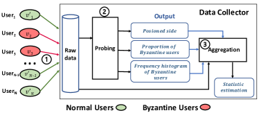
Figure 1: System model and aggregation framework

IV A Baseline Protocol for Mean Estimation

This section proposes a baseline protocol for numerical mean aggregation against Biased Byzantine Attacks (and thus General Byzantine Attacks). For the collector to probe and aggregate the mean, each user perturbs her numerical value twice with $\epsilon_{\alpha}$ and $\epsilon_{\beta}$ budgets respectively by an LDP perturbation mechanism. Here $\epsilon_{\alpha}+\epsilon_{\beta}=\epsilon$, the overall privacy budget, and $\epsilon_{\alpha}\ll\epsilon_{\beta}$. Upon receiving the two perturbed data sets $V^{\prime}({\alpha})$ and $V^{\prime}({\beta})$, the collector first probes on $V^{\prime}({\alpha})$ for the three features of Byzantine users using Expectation-Maximization Filter (EMF), which will be elaborated in Section IV-B. Based on these features, the collector then estimates the mean from $V^{\prime}({\beta})$. In addition, since EMF can only probe on Biased Byzantine Attacks, we also need to have an initial guess on the true mean $O$. In the rest of this section, we first describe how to initialize $O$, and then present the EMF algorithm and mean estimation. In what follows we illustrate our algorithms using Piecewise Mechanism (PM) as the perturbation mechanism, and thus the perturbed value domain $[D_{L},D_{R}]$ becomes $[-C,C]$.

IV-A Initializing True Mean $O$

According to Definition 4, an initial true mean $O$ is needed to define a Biased Byzantine Attack. In essence, $O$ narrows down the poison values as in BBA they can only appear on one side of $O$. In order not to exclude potential poison values from our analysis, we should have a pessimistic initialization of $O$ as $O^{\prime}$ so that $O^{\prime}\leq O$ if the poisoned side is on the right and vice versa. As such, the poison values’ range of the true general Byzantine attack is a subset of that of the BBA in our analysis. The following theorem provides such a pessimistic initialization $O^{\prime}$.

Theorem 2.

Given a collected value set $V^{\prime}$ and an upper bound of Byzantine user proportion $\gamma_{sup}$, let $V^{\prime}_{B}$ denote the set of poison values, and $T$ denote the set of the largest $\lceil\gamma_{sup}\cdot N\rceil$ values in $V^{\prime}$. The following $O^{\prime}$ is a pessimistic initialization of $O$, i.e., $O^{\prime}\leq O$ if the poisoned side is on the right and vice versa.

$$\begin{split}O^{\prime}=\frac{1}{1-\gamma_{sup}}(\sum\limits_{v^{\prime}_{i}\in V^{\prime}}v^{\prime}_{i}-\sum\limits_{v^{\prime}_{j}\in T}v^{\prime}_{j})\end{split}$$

Proof.

The true mean $O$ can be obtained by removing the effect of $Y$ from $V^{\prime}$:

$$O=\frac{\sum\limits_{v^{\prime}_{i}\in V^{\prime}}v^{\prime}_{i}-\sum\limits_{v^{\prime}_{j}\in V^{\prime}_{B}}v^{\prime}_{j}}{1-\gamma}.$$ (6)

Likewise, we can obtain $O^{\prime}$ from removing the effect of $T$:

$$O^{\prime}=\frac{\sum\limits_{v^{\prime}_{i}\in V^{\prime}}v^{\prime}_{i}-\sum\limits_{v^{\prime}_{j}\in T}v^{\prime}_{j}}{1-\gamma_{sup}}.$$ (7)

Since the values in $T$ are the largest $\gamma_{sup}$ in $Y$, so we have

$$\sum\limits_{v^{\prime}_{i}\in T}v^{\prime}_{i}\geq\sum\limits_{v^{\prime}_{j}\in V^{\prime}_{B}}v^{\prime}_{j}$$

Compare Equ. 6 and Equ. 7, we have $O^{\prime}\leq O$. ∎

According to our threat model, $\gamma_{sup}=0.5$ by default, and can be further reduced with prior knowledge. For ease of presentation, in the rest of this paper we simply set $O^{\prime}=0$ unless otherwise stated and use the right hand side as the poisoned side.

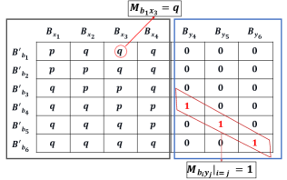
Figure 2: Transform matrix M

IV-B Expectation-Maximization Filter

Recall that normal users perturb their values by using Piecewise Mechanism in Algorithm 1, whereas a biased Byzantine attacker chooses and sends a poison value directly. Such difference inspires us to reconstruct the original distribution and then probe some features of Byzantine users. Hereafter, we present a novel algorithm, namely the Expectation-Maximization Filter (EMF), to estimate such information by Maximum Likelihood Estimation (MLE) [39].

Let $V=\{v_{1},v_{2},...,v_{N}\}$ denote the original values of users, and $V^{\prime}=\{v_{1}^{{}^{\prime}},v_{2}^{{}^{\prime}},...,v_{N}^{{}^{\prime}}\}$ denote the collected ones. Since the probing only needs coarse precision, we discretise the original value domain $[-1,1]$ and perturbed value domain $[-C,C]$, respectively. Specifically, the former is discretised into $d$ buckets, and $d^{\prime}$ for the latter, so let $\textbf{x}=\{x_{1},...,x_{d}\}$ denote the frequency histogram of normal users in buckets $B_{x}=\{B_{x_{1}},...,B_{x_{d}}\}$, and $\{b_{1},...,b_{d^{\prime}}\}$ denote those in buckets $B^{\prime}=\{B^{\prime}_{b_{1}},...,B^{\prime}_{b_{d}}\}$, respectively. Recall that $O^{\prime}=0$, so the poison values will only appear in the right half of the perturbed domain $[0,C]$ with $d^{\prime}/2$ buckets. Let $\textbf{y}=\{y_{d^{\prime}/2+1},...,y_{d^{\prime}}\}$ denote the frequency histogram of Byzantine users in buckets $B_{y}=\{B_{y_{d^{\prime}/2}},...,B_{y_{d^{\prime}}}\}$.

With that said, the objective of EMF is to reconstruct the frequency histogram $F$, which comprises of the frequency counts of both normal users x and poison values y in the original value domain. That is, $F=\{\textbf{x,\ y}\}=\{x_{1},...,x_{k},...,x_{d},y_{d^{\prime}/2+1},...,y_{j},...,y_{d^{\prime}}\}$. To adopt MLE, we obtain the log-likelihood function of $F$ as follows:

$$\begin{split}&l(F)=lnPr[V^{{}^{\prime}}|F]=ln\prod_{i=1}^{N}Pr[v_{i}^{\prime}|F]=\\ &\sum_{i=1}^{N}ln(\sum_{k=1}^{d}x_{k}Pr[v^{\prime}_{i}|v_{i}\in B_{x_{k}}]+\!\sum_{j=d^{\prime}/2+1}^{d^{\prime}}\!y_{j}Pr[v^{\prime}_{i}|v_{i}\in B_{y_{j}}])\end{split}$$ (8)

where $Pr[v^{\prime}_{i}|v_{i}\in B_{x_{k}}]$ and $Pr[v^{\prime}_{i}|v_{i}\in B_{y_{j}}]$ are constants, thus $l(F)$ is a concave function and EM algorithm can converge to the maximum likelihood estimator [6].

To facilitate the derivation, we use a transform matrix M to capture the transformation probabilities $Pr[v^{\prime}_{i}|v_{i}]$ for users. As shown in Fig. 2, M is a $d^{\prime}\times(d+d^{\prime}/2)$ matrix with all elements values in $[0,1]$. It consists of two parts. The left-hand side is a $d^{\prime}\times d$ matrix for normal users, where $M_{b_{i}x_{k}}=Pr[v^{\prime}_{i}\in B_{b_{i}}|v_{i}\in B_{x_{k}}]$. Given the original value $v$ of a normal user and a privacy budget $\epsilon$, let $p$ denote the probability that the perturbed value $v^{\prime}$ falls in a bucket of $[l(v),r(v)]$ in Algorithm 1, and $q$ otherwise. For example, in Fig. 2, given an original value in bucket $B_{x_{3}}$, $M_{b_{1}x_{3}}=q$ denotes the conditional probability that the output falls into bucket $B^{\prime}_{b_{1}}$ is $q$. The right-hand side of M is a $d^{\prime}\times(d^{\prime}/2)$ matrix for poison values, and likewise, $M_{b_{i}y_{j}}=Pr[v^{\prime}_{i}\in B_{b_{i}}|v_{i}\in B_{y_{j}}]$. Since Byzantine users send poison values directly to the data collector, $M_{b_{i}y_{j}}=1$ when $i=j$, and $M_{b_{i}y_{j}}=0$ when $i\neq j$.

Now that the transform matrix M is derived, the EMF algorithm reconstructs the frequency histogram ($\hat{x}$ for normal values and $\hat{y}$ for poison values) as illustrated in Algorithm 2, which can be derived using the methodology described in the literature [39]. Note that $c_{i}$ in $E$-step denotes the count of perturbed values from $V^{\prime}$ in bucket $B^{\prime}_{b_{i}}$. First, the algorithm assigns some non-zero initial values to $\hat{x}$ and $\hat{y}$, subject to $\hat{x}+\hat{y}=1$ (line 1). Next, it executes the EM algorithm, alternating the $E$-step and the $M$-step. The $E$-step evaluates the log-likelihood expectation by the observed counts $c_{i}$ and the current $\hat{x}$ and $\hat{y}$ (lines 3-9), and the $M$-step calculates $\hat{x}$ and $\hat{y}$ that maximize the expected likelihood (lines 10-15) as inputs for the next round $E$-step. Finally, the algorithm returns the estimated frequency histogram $\hat{x}$ and $\hat{y}$ when the convergence condition is met (line 16).

Algorithm 2 Expectation-Maximization Filter (EMF)

Input: Transform matrix M and collected values $V^{\prime}$

Output: $\hat{x}$, $\hat{y}$

1:Initialization: $\hat{x_{k}}=\hat{y_{j}}=\frac{1}{d+d^{\prime}/2}$

2:while not converge do

3:    E-step: $\forall\ k\in\{1,...,d/2\}$

4:    $P_{x_{k}}=\hat{x_{k}}\sum_{i=1}^{d^{\prime}}c_{i}\frac{M_{b_{i}x_{k}}}{\sum_{t=1}^{d}M_{b_{i}x_{t}}\hat{x_{t}}}$

5:    $\forall\ k\in\{d/2+1,...,d\}$

6:    $P_{x_{k}}=\hat{x_{k}}\sum_{i=1}^{d^{\prime}}c_{i}\frac{M_{b_{i}x_{k}}}{\sum_{t=1}^{d}M_{b_{i}x_{t}}\hat{x_{t}}+M_{b_{i}y_{i}}\hat{y_{i}}}$

7:    $\forall\ j\in\{d^{\prime}/2+1,...,d^{\prime}\}$

8:    $P_{y_{j}}=\hat{y_{j}}\sum_{i=1}^{d^{\prime}}c_{i}\frac{M_{b_{i}y_{j}}}{\sum_{t=1}^{d}M_{b_{i}x_{t}}\hat{x_{t}}+M_{b_{i}y_{i}}\hat{y_{i}}}$

9:    M-step: $\forall\ k\in\{1,...,d\}$

10:    $\hat{x_{k}}=\frac{P_{x_{k}}}{\sum_{i=1}^{d}P_{x_{i}}+\sum_{j=d^{\prime}/2+1}^{d^{\prime}}P_{y_{j}}}$

11:    $\forall\ j\in\{d^{\prime}/2+1,...,d^{\prime}\}$

12:    $\hat{y_{j}}=\frac{P_{y_{j}}}{\sum_{k=1}^{d}P_{x_{k}}+\sum_{i=d^{\prime}/2+1}^{d^{\prime}}P_{y_{i}}}$

13:return $\hat{x}$, $\hat{y}$

IV-C Byzantine Feature Estimation

The outputs of EMF $\hat{x}$ and $\hat{y}$ on the collected value set $V^{\prime}$ is used to probe Byzantine users’ features. The first feature is the poisoned side $\mathcal{S}$, and the pseudo-code is shown in Algorithm 3. First, it applies EMF separately to the transform matrices $\textbf{M}_{R}$ and $\textbf{M}_{L}$ (lines 1-2). If the probing range is $[0,C]$, $\textbf{M}_{R}$ is used with buckets $\{B_{y_{d^{\prime}/2+1}},...,B_{y_{d^{\prime}}}\}$ in the right-hand matrix of M for poison values; otherwise $\textbf{M}_{L}$ is used with buckets $\{B_{y_{1}},...,B_{y_{d^{\prime}/2}}\}$. Then, to determine which side is more probable, it calculates the variance of $\hat{x_{L}}$ and $\hat{x_{R}}$ (lines 3-4), where $\hat{x_{L}}$ (resp. $\hat{x_{R}}$) denotes the frequency histogram for normal users when the input matrix is $\textbf{M}_{L}$ (resp. $\textbf{M}_{R}$). Finally, it chooses the poisoned side with a lower variance (lines 5-8).

Algorithm 3 Poisoned Side Probing

Input: Transform matrix $\textbf{M}_{L}$, transform matrix $\textbf{M}_{R}$ and collected values $V^{\prime}$

Output: Poisoned side $\mathcal{S}$

1:$(\hat{x_{L}},\hat{y_{L}})=EMF(\textbf{M}_{L},V^{\prime})$;

2:$(\hat{x_{R}},\hat{y_{R}})=EMF(\textbf{M}_{R},V^{\prime})$;

3:$Var_{L}=Variance(\hat{x_{L}})$;

4:$Var_{R}=Variance(\hat{x_{R}})$;

5:if $Var_{L}<Var_{R}$ then return $Left\ side$

6:else return $Right\ side$

Upon knowing the poisoned side, we can now determine the remaining two features. The second one of Byzantine users is the frequency histogram $\hat{y}$ of poison values which can be chosen from $\hat{y_{L}}$ or $\hat{y_{R}}$ in Algorithm 3 accordingly. The third one is the proportion of Byzantine users $\hat{\gamma}$, which can be derived from $\hat{y}$, the estimated frequency histogram of poison values by EMF:

$$\hat{\gamma}=\sum_{j=d^{\prime}/2+1}^{d^{\prime}}{\hat{y_{j}}}=\frac{\hat{m}}{N}\approx\frac{m}{N}=\gamma,$$ (9)

where $\hat{m}$ denotes the estimated number of Byzantine users, and $\gamma$ denotes the true proportion of Byzantine users.

When $\epsilon\rightarrow 0$, the estimated frequency histogram $\hat{x}$ of normal users converges to a uniform distribution, whereas that of Byzantine users $\hat{y}$ converges to the true distribution of poison values. This, along with the correctness of Algorithm 3 and Equ. 9, can be proved by the following theorem.

Theorem 3.

Let $a=\{a_{d^{\prime}/2+1},...,a_{d^{\prime}}\}$ denote the count of poison values in buckets $\{B_{d^{\prime}/2+1},...,B_{d^{\prime}}\}$. When $\epsilon\rightarrow 0$, the convergence results are $\hat{x_{k}}=\frac{n}{Nd}(k\in\{1,...,d^{\prime}\})$ and $\hat{y_{j}}=\frac{a_{j}}{N}(j\in\{d^{\prime}/2+1,...,d^{\prime}\})$.

Proof.

When $\epsilon\rightarrow 0$, all inputs from normal users are equally perturbed into $d^{\prime}$ buckets with probability $\frac{1}{d^{\prime}}$, which leads to a uniform distribution. Let $a=\{a_{d^{\prime}/2+1},...,a_{t},...,a_{d^{\prime}}\}$ denote the count of poison values in corresponding buckets $B^{\prime}_{b_{i}}$, and we have $c_{t}\rightarrow\frac{n}{d^{\prime}},t\in\{1,...,d^{\prime}/2\}$ and $c_{t}\rightarrow\frac{n}{d^{\prime}}+a_{t},t\in\{d^{\prime}/2+1,...,d^{\prime}\}$.

Note that $\sum_{k=1}^{d}\hat{x_{k}}+\sum_{j=d^{\prime}/2+1}^{d^{\prime}}\hat{y_{j}}=1$, the Lagrangian function of Equ. 8 can be written as:

$$L(F)=l(F)+\omega(\sum_{k=1}^{d}\hat{x_{k}}+\sum_{j={d^{\prime}/2+1}}^{d^{\prime}}\hat{y_{j}}-1).$$

Let all first-order partial derivatives of L w.r.t. $\hat{x_{k}}$ and $\hat{y_{j}}$ equal zero

$$\begin{split}&\frac{\partial L(F)}{\partial\hat{x_{k}}}=\sum_{t=1}^{d^{\prime}}c_{t}\frac{\frac{1}{d^{\prime}}}{\sum_{k=1}^{d}\hat{x_{k}}\frac{1}{d^{\prime}}}+\omega,\ k\in\{1,...,\frac{d}{2}\}\\ &\frac{\partial L(F)}{\partial\hat{x_{k}}}=\sum_{t=1}^{d^{\prime}}c_{t}\frac{\frac{1}{d^{\prime}}}{\sum_{k=1}^{d}\hat{x_{k}}\frac{1}{d^{\prime}}+\hat{y_{t}}}+\omega,\ k\in\{\frac{d}{2}+1,...,d\}\\ &\frac{\partial L(F)}{\partial\hat{y_{j}}}=c_{j}\frac{1}{\sum_{k=1}^{d}\hat{x_{k}}\frac{1}{d^{\prime}}+\hat{y_{j}}}+\omega,\ j\in\{\frac{d^{\prime}}{2}+1,...,d^{\prime}\}\end{split}$$

we have:

$$\hat{x_{k}}\rightarrow\frac{n}{Nd},\ \ \hat{y_{j}}\rightarrow\frac{a_{j}}{N},j\in\{d^{\prime}/2+1,...,d^{\prime}\},\ \omega\rightarrow-N.$$ (10)

According to Equ. 10, the frequency histogram $\hat{x}$ of normal users converges to a uniform distribution, whereas that of Byzantine users $\hat{y}$ converges to the true distribution of poison values. ∎

When $\epsilon\rightarrow 0$, $\hat{y}$ converges to the true distribution of poison values, so Equ. 9 can well estimate the proportion of Byzantine users. The fact that $\hat{x}$ converges to a uniform distribution explains the correctness of Algorithm 3 — if we choose the correct side (say, the right side), the distribution of $\hat{x}$ should be a uniform distribution with a very small variance; If we select the left side and use $M_{L}$ as the EMF input, only collected values from $[-C,0]$ can converge into $B_{y_{i}}$. Therefore, poison values in $[0,C]$ can only converge to $B_{x_{i}}$, which are regarded as normal values. The convergence result $\hat{x_{L}}$ will be biased towards $[0,C]$, which is far from a uniform distribution. In this case, the variance of $\hat{x}$ appears to be far greater than selecting the reverse side.

Since $\epsilon_{\alpha}\ll\epsilon_{\beta}$, we choose $V^{\prime}(\alpha)$ over $V^{\prime}(\beta)$ to probe Byzantine features, which is more accurate than using the latter according to Theorem 3.

IV-D Mean Estimation

Now that we have probed the features of Byzantine users from $V^{\prime}(\alpha)$, we can leverage them to estimate the mean in $V^{\prime}(\beta)$. Since the poison values in $V^{\prime}(\alpha)$ and $V^{\prime}(\beta)$ form a unified attack, their deviation $D$ from the true mean $O$ is assumed the same. Therefore, we have:

$$\begin{split}D=\frac{m(\mathbb{M}_{\alpha}-O)}{N}=\frac{m(\mathbb{M}_{\beta}-O)}{N},\end{split}$$

where $\mathbb{M}_{\alpha}$ denotes the mean of poison values in $V^{\prime}(\alpha)$, and $\mathbb{M}_{\beta}$ for $V^{\prime}(\beta)$. Thus, $\mathbb{M}_{\alpha}=\mathbb{M}_{\beta}$.

$\mathbb{M}_{\alpha}$ can be obtained from the frequency histogram estimation $\widehat{y(\alpha)}$, i.e., the convergence result for poison values of $V^{\prime}(\alpha)$:

$$\begin{split}\mathbb{M}_{\alpha}=\frac{\sum\widehat{y_{j}({\alpha})}\nu_{j}}{\sum\widehat{y_{j}({\alpha})}},\ j\in\{d^{\prime}/2+1,...,d^{\prime}\},\end{split}$$ (11)

where $\nu_{j}$ denotes the median value of $B_{y_{j}}$.

Because the perturbed mean gained from PM is an unbiased estimation of the original one, the mean $\widetilde{M}$ of normal users with $\epsilon_{\beta}$ can be derived as:

$$\widetilde{M}=\frac{\sum\limits_{v^{\prime}({\beta)}\in V^{\prime}({\beta})}{v^{\prime}({\beta})}-\hat{m}\mathbb{M}_{\beta}}{N-\hat{m}}.$$ (12)

Substitute Equ. 11 into Equ. 12. Notice that $\mathbb{M}_{\alpha}=\mathbb{M}_{\beta}$, $\widetilde{M}$ can be written as:

$$\begin{split}\widetilde{M}=\frac{\sum\limits_{v^{\prime}({\beta)}\in V^{\prime}({\beta})}{v^{\prime}({\beta})}-\hat{m}\frac{\sum\widehat{y_{j}({\alpha})}\nu_{j}}{\sum\widehat{y_{j}({\alpha})}}}{N-\hat{m}},\ j\in\{d^{\prime}/2+1,...,d^{\prime}\}.\end{split}$$

V Differential Aggregation Protocol

The baseline protocol has one flaw as they may choose to send some normal values at $\epsilon_{\alpha}$ to hide their attacking intention, and send poison values at $\epsilon_{\beta}$. Since the probed Byzantine features become less accurate, the accuracy of the mean estimation is degraded significantly. In essence, this flaw is caused by two separate and fixed $\epsilon$’s in the baseline protocol, so Byzantine users can easily tell the smaller one is $\epsilon_{\alpha}$ and serves for probing Byzantine features, whereas the larger one serves for statistics estimation.

This motivates us to enhance the baseline protocol with a single but random $\epsilon$. In this section, we present a multi-group collection mechanism, namely Differential Aggregation Protocol (DAP). Our idea is to randomly assign users into $h$ groups, each with its own $\epsilon$ setting. The collector performs EMF in each group to probe Byzantine users’ features, as in the baseline protocol. And then the collector estimates a mean from each group, based on which an inter-group mean is aggregated. There are a few advantages. First, Byzantine users cannot differentiate if their values are used for probing or estimation and thus take the above strategy. Second, there is no need to split privacy budgets for users, which can improve the estimation accuracy. Third, this protocol can naturally handle users with different privacy budgets.

As illustrated in Fig. 3, the workflow of the DAP protocol has five stages:

1. Grouping. The data collector allocates users into groups and assigns each group with a dedicated privacy budget.

2. Perturbation. Users in each group perturb their values according to their assigned privacy budgets and send them to the data collector.

3. Probing. The data collector executes the EMF algorithm for each group to probe the Byzantine features.

4. Intra-group Estimation. The data collector attains a mean from each group from the output of EMF.

5. Inter-group Aggregation. The data collector combines estimated means from all groups into one.

Figure 3: Differential Aggregation Protocol

V-A Grouping

First of all, the data collector determines a minimal acceptable privacy budget $\epsilon_{0}$ to bound the perturbation noise of normal values according to the privacy budget $\epsilon$ for users. Then data collector creates $h=\lceil log_{2}(\epsilon/\epsilon_{0})\rceil+1$ equal-sized groups, denoted by $\{G_{1},...,G_{t},...,G_{h}\}$, with decreasing budgets $\{\epsilon,\frac{1}{2}\epsilon,\frac{1}{4}\epsilon,...,\epsilon_{t},...,\epsilon_{0}\}$. Users are randomly assigned to the groups by the collector and perturb their values according to the $\epsilon_{t}$ of the groups they belong to. To guarantee all users have the same privacy budget, those assigned with smaller $\epsilon_{t}$ perturb and report multiple times until the overall privacy budget is depleted. Let $V^{\prime}_{t}$ denote the collected values from group $G_{t}$ and $N_{t}=\frac{\epsilon N}{\epsilon_{t}h}$ denote the number of collected values from group $G_{t}$.

V-B Intra-group Mean Estimation

Upon collecting all perturbed values, we carry out EMF in each group to probe the Byzantine users’ features from the frequency histogram, as described in Section IV. Specifically, we can obtain the poisoned side, the proportion of Byzantine users and the frequency histogram of poison values $\widehat{y(t)}$ in $G_{t}$. As such, the mean $M_{t}$ of group $G_{t}$ with privacy budget $\epsilon_{t}$, can be estimated by removing poison values:

$$M_{t}=\frac{\sum\limits_{v^{\prime}_{t}\in V^{\prime}_{t}}{v^{\prime}_{t}}-\hat{m_{t}}\sum_{j=d^{\prime}/2+1}^{d^{\prime}}(\widehat{y_{j}(t)}\nu_{j})}{N_{t}-\hat{m_{t}}},$$ (13)

where $\widehat{y_{j}(t)}\in\widehat{y(t)}$, $\hat{m_{t}}=N_{t}\sum{\widehat{y(t)}}$ and $\nu_{j}$ denotes the median value of $B_{y_{j}}$.

However, according to Theorem 3, both $\hat{y_{t}}$ and $\hat{m_{t}}$ become less accurate as the user population is diluted by grouping, especially when the $\epsilon_{t}$ of a group is large. Hereafter, we propose two post-processing schemes, namely, EMF* and CEMF*, to further enhance the accuracy of convergence results and mean estimation in Equ. 13 in each group.

EMF*. It utilizes the proportion of Byzantine users $\hat{\gamma}$ (with small $\epsilon_{t}$) probed from EMF to improve the convergence process, by imposing $\sum\hat{y}=\hat{\gamma}$, $\sum\hat{x}=1-\hat{\gamma}$ as two additional conditions to satisfy in EMF. Accordingly, the maximization problem in M steps of EMF becomes:

$$\begin{split}&\mathop{\arg\max}\limits_{\hat{x},\hat{y}}\ \sum_{k=1}^{d}P_{x_{k}}ln\hat{x_{k}}+\sum_{j=d^{\prime}/2+1}^{d^{\prime}}P_{y_{j}}ln\hat{y_{j}},\\ &subject\ to\ \sum_{k=1}^{d}\hat{x_{k}}=1-\hat{\gamma},\ \sum_{j=d^{\prime}/2+1}^{d^{\prime}}\hat{y_{j}}=\hat{\gamma}\end{split}$$ (14)

EMF* can improve EMF in terms of the accuracy of converged poison value histogram because the additional restrictions eliminate those infeasible poison values. To resolve Equ. 14, we have the following theorem.

Theorem 4.

The maximum in Equ. 14 is reached when the output frequency histograms are

$$\hat{x_{k}}=(1-\hat{\gamma})\frac{Px_{k}}{\sum_{k=1}^{d}{Px_{k}}},\ \hat{y_{j}}=\hat{\gamma}\frac{Py_{j}}{\sum_{j=d^{\prime}/2+1}^{d^{\prime}}{Py_{j}}}.$$

Algorithm 4 EMF with Restrictions (EMF*)

Input: Transform matrix M, collected values $V^{\prime}$, the estimated proportion of Byzantine users $\hat{\gamma}$

Output: $\hat{x},\hat{y}$

1:Initialization: $\hat{x_{k}}=\hat{y_{j}}=\frac{1}{d+d^{\prime}/2}$

2:while not converge do

3:    E-step:

4:     Same as the E-step in EMF in Algorithm 2

5:    M-step:

6:    $\forall\ k\in\{1,...,d\}$

7:    $\hat{x_{k}}=(1-\hat{\gamma})\frac{P_{x_{k}}}{\sum_{i=1}^{d}P_{x_{i}}}$

8:    $\forall\ j\in\{d^{\prime}/2+1,...,d^{\prime}\}$

9:    $\hat{y_{j}}=\hat{\gamma}\frac{P_{y_{j}}}{\sum_{i=d^{\prime}/2+1}^{d^{\prime}}P_{y_{i}}}$

10:return $\hat{x},\hat{y}$

Proof.

We apply Lagrangian multiplier method to derive maximal value of Euq. 14. Let

$$\begin{split}\mathcal{L}&=\sum_{k=1}^{d}P_{x_{k}}ln\hat{x_{k}}+\sum_{j=d^{\prime}/2+1}^{d^{\prime}}P_{y_{j}}ln\hat{y_{j}}\\ &+\lambda_{1}(\sum_{k=1}^{d}\hat{x_{k}}-1+\hat{\gamma})+\lambda_{2}(\sum_{j=d^{\prime}/2+1}^{d^{\prime}}\hat{y_{j}}-\hat{\gamma}),\end{split}$$

where $\lambda_{1}$ and $\lambda_{2}$ are two constants and the first-order partial derivatives of $\mathcal{L}$ w.r.t. $\hat{x_{k}}$ and $\hat{y_{j}}$ are

$$\frac{\partial\mathcal{L}}{\partial\hat{x_{k}}}=\frac{P_{x_{k}}}{\hat{x_{k}}}+\lambda_{1},\ \frac{\partial\mathcal{L}}{\partial\hat{y_{j}}}=\frac{P_{y_{j}}}{\hat{y_{j}}}+\lambda_{2}.$$

Let $\frac{\partial l}{\partial\hat{x_{k}}}$ and $\frac{\partial l}{\partial\hat{y_{j}}}$ be zero, and we have

$$P_{x_{k}}+\lambda_{1}\hat{x_{k}}=0,\ P_{y_{j}}+\lambda_{2}\hat{y_{j}}=0.$$ (15)

From the restrictions in Equ. 14, we can deduce that

$$\lambda_{1}=\frac{\sum_{i=1}^{d}P_{x_{i}}}{\hat{\gamma}-1},\ \lambda_{2}=\frac{\sum_{i=d^{\prime}/2+1}^{d^{\prime}}P_{y_{i}}}{-\hat{\gamma}}.$$

Replacing them in Equ. 15, we can reach that

$$\hat{x_{k}}=(1-\hat{\gamma})\frac{Px_{k}}{\sum_{i=1}^{d}P_{x_{i}}},\ \hat{y_{j}}=\hat{\gamma}\frac{Py_{j}}{\sum_{i=d^{\prime}/2+1}^{d^{\prime}}P_{y_{i}}}.$$

∎

Algorithm 4 shows the pseudo-code of EMF*, where the M-step from EMF has been modified with the results of Theorem 4. Note that instead of replacing EMF, EMF* is a post-processing of EMF, as the former needs the $\hat{\gamma}$ of latter as input.

CEMF*. This post-processing further considers a common scenario where Byzantine users inject poison values into a small domain only. In such cases, the mean estimation from EMF and EMF* is relatively poor since the frequency counts of some buckets in the histogram can be extremely high, which cannot be restored very accurately by EMF/EMF*. As such, we propose an alternative post-processing, namely EMF* with concentration (CEMF*) by suppressing those buckets $B_{y_{j}}$ with small frequency counts $\hat{y_{j}}$ in EMF’s output. That is, we treat these buckets as if no poison values are there. Let $\mathcal{B}$ denote the set of buckets for poison values that are chosen by Byzantine users, and $\overline{\mathcal{B}}$ denote the set of remaining buckets. Here we suppress all buckets in $\overline{\mathcal{B}}$ first, which will be proved to achieve the optimal performance later in Theorem 5. The log-likelihood function then becomes:

$$\begin{split}&l(F)=lnPr[V^{{}^{\prime}}|F]=ln\prod_{i=1}^{N}Pr[v_{i}^{\prime}|F]=\\ &\sum_{i=1}^{N}ln(\sum_{k=1}^{d}\hat{x_{k}}Pr[v^{\prime}_{i}|v_{i}\in B_{x_{k}}]+\sum_{B_{y_{j}}\in\mathcal{B}}\hat{y_{j}}Pr[v^{\prime}_{i}|v_{i}\in B_{y_{j}}]).\\ \end{split}$$

Our objective is to maximize $l(F)$, subject to $\sum_{k=1}^{d}\hat{x_{k}}=1-\hat{\gamma}$ and $\sum_{B_{y_{j}}\in\mathcal{B}}\hat{y_{j}}=\hat{\gamma}$. The maximization can be obtained following Algorithm 4, by initially setting $\hat{y_{i}}=0$ (i.e., those buckets in $\overline{\mathcal{B}}$).

The following theorem shows CEMF* can improve the estimation accuracy if we have the knowledge about $\overline{\mathcal{B}}$ and suppress some buckets inside. Specifically, CEMF* achieves its optimal performance when all buckets in $\overline{\mathcal{B}}$ are suppressed:

Theorem 5.

The converged frequency histograms monotonically approach the actual ones with respect to $||\overline{\mathcal{B}}||$, the number of suppressed buckets.

Proof.

Let $\mathcal{B}=\{B_{y_{1}},...,B_{y_{t}}\}$, and $\overline{\mathcal{B}}=\{B_{y_{t+1}},...,B_{y_{d^{\prime}}}\}$. We start from the state where all buckets hold non-zero values, i.e., $B_{y_{i}}\neq 0,i\in\{1,...,d^{\prime}\}$, and reconstruct the frequency histogram for poison values in $[-C,C]$. The likelihood estimator in Equ. 8 becomes

$$\begin{split}l(F)&=\sum_{i=1}^{N}ln(\sum_{k=1}^{d}\hat{x_{k}}Pr[v_{i}^{\prime}|v_{i}\in B_{x_{k}}]\\ &+\sum_{j=1}^{d^{\prime}}\hat{y_{j}}Pr[v_{i}^{\prime}|v_{i}\in B_{y_{j}}])\\ &=\sum_{t=1}^{d^{\prime}}c_{t}ln(\sum_{k=1}^{d}\hat{x_{k}}M_{b_{t}x_{k}}+\sum_{j=1}^{d^{\prime}}\hat{y_{j}}M_{b_{t}y_{j}}).\end{split}$$

Note that $\sum_{k=1}^{d}\hat{x_{k}}+\sum_{j=1}^{d^{\prime}}\hat{y_{j}}=1$, we employ the Lagrangian multiplier method to derive the extremum. The Lagrangian function can be written as:

$$L(F)=l(F)+\lambda(\sum_{k=1}^{d}\hat{x_{k}}+\sum_{j=1}^{d^{\prime}}\hat{y_{j}}-1).$$

Let all first-order partial derivatives of L w.r.t. $\hat{x_{k}}$ and $\hat{y_{j}}$ equal zero

$$\begin{split}&\frac{\partial L(F)}{\partial\hat{x_{k}}}=\sum_{t=1}^{d^{\prime}}\frac{c_{t}M_{b_{t}x_{k}}}{\sum_{k=1}^{d}\hat{x_{k}}M_{b_{t}x_{k}}+\hat{y_{t}}}+\lambda=0,\ k\in\{1,...,d\}\\ &\frac{\partial L(F)}{\partial\hat{y_{j}}}=\sum_{t=1}^{d^{\prime}}\frac{c_{t}M_{b_{t}y_{j}}}{\sum_{k=1}^{d}\hat{x_{k}}M_{b_{t}x_{k}}+\hat{y_{t}}}+\lambda=0,\ j\in\{1,...,d^{\prime}\}\end{split}$$

we have:

$$\hat{x_{k}}=0,\ k\in\{1,...,d\},\ \ \hat{y_{j}}=\frac{c_{j}}{N},\ j\in\{1,...,d^{\prime}\},\ \lambda=-N.$$

This result shows all collected values converge to poison values if no bucket is suppressed, and we can obtain:

$$(\sum_{k=1}^{d}\hat{x_{k}}+\sum_{j=1}^{t}\hat{y_{j}})\bigg{|}_{y_{i}\neq 0,i\in\{1,...,d^{\prime}\}}=\sum_{j=1}^{t}\frac{c_{j}}{N}.$$

When we suppress the bucket $B_{y_{d^{\prime}}}$ (by setting $\hat{y_{d^{\prime}}}=0$) and carry out EMF, the collected values in $B^{\prime}_{b_{d^{\prime}}}$ can only converge to $B_{x_{k}}(k\in\{1,...,d\})$, but not $B_{y_{j}}(j\in\{1,...,d^{\prime}\})$. Hence, every $\hat{x_{k}}$ will increase. Therefore, suppressing $B_{y_{d^{\prime}}}$ leads to the increase of all $\hat{x_{k}}$, which in turn results in the decrease of all $\hat{y_{j}}$. However, since the decrease of $\hat{y_{j}}(j\in\{1,...,t\})$ is a part of increment of $\hat{x}$, we can figure out $(\sum_{k=1}^{d}\hat{x_{k}}+\sum_{j=1}^{t}\hat{y_{j}})\bigg{|}_{y_{i}\neq 0,i\in\{1,...,d^{\prime}\}}\leq(\sum_{k=1}^{d}\hat{x_{k}}+\sum_{j=1}^{t}\hat{y_{j}})\bigg{|}_{y_{d^{\prime}}=0}$. Suppress all buckets one by one in $\overline{\mathcal{B}}$ similarly, we have:
$(\sum_{k=1}^{d}\hat{x_{k}}+\sum_{j=1}^{t}\hat{y_{j}})\bigg{|}_{y_{i}\neq 0,i\in\{1,...,d^{\prime}\}}\leq(\sum_{k=1}^{d}\hat{x_{k}}+\sum_{j=1}^{t}\hat{y_{j}})\bigg{|}_{y_{d^{\prime}}=0}\\ \leq...\leq(\sum_{k=1}^{d}\hat{x_{k}}+\sum_{j=1}^{t}\hat{y_{j}})\bigg{|}_{y_{d^{\prime}}=0,...,y_{t+1}=0}.$

When the number of suppressed buckets in $\overline{\mathcal{B}}$ increases, the corresponding interference of $\overline{\mathcal{B}}$ decreases. Therefore, the collected values more accurately converge to the buckets that they should belong to, and thus achieve a better convergence result.

After suppressing all buckets in $\overline{\mathcal{B}}$, all collected values will convergence to normal values and poison values in $B_{y_{j}}(j\in{1,...,t})$ and we can infer that$(\sum_{k=1}^{d}\hat{x_{k}}+\sum_{j=1}^{t}\hat{y_{j}})\bigg{|}_{y_{d^{\prime}}=0,...,y_{t+1}=0}=1,$ which is the optimal case where none of the collected values will converge to buckets in $\overline{\mathcal{B}}$. ∎

V-C Aggregating Inter-group Estimations

After intra-group mean estimations, we finally combine all these estimated means into a single mean. However, the naive method of averaging all of them in equal weights does not provide the optimal data utility — values perturbed with larger $\epsilon_{t}$ have higher accuracy. Hence, the group they belong to deserves higher weight. At the end of this section, inspired by [72], we propose an aggregation strategy that can linearly combine all estimated intra-group mean values $\{M_{1},...,M_{t},...,M_{h}\}$ into $\tilde{M}$, while achieving minimal overall variance. Since the variance is related to the true value that we don’t know, we thus only consider the minimal variance under the worst-case, i.e., when all the original values are either -1 or 1.

Algorithm 5 Mean Aggregation

Input: Mean values $\{M_{1},...,M_{t},...,M_{h}\}$, privacy budgets $\{\epsilon_{1},...,\epsilon_{t},...,\epsilon_{h}$} and the estimated numbers of normal users $\{\hat{n_{1}},...,\hat{n_{t}},...,\hat{n_{h}}$}

Output: The aggregated mean $\tilde{M}$

1:Initialization: $w_{t}=0,\ t=\{1,2,...,h\}$

2:for $t=1\ to\ h$ do

3:    $w_{t}=[B_{t}\sum_{i=1}^{h}\frac{1}{B_{i}}]^{-1}$, $B_{t}=\hat{n_{t}}(\frac{1}{e^{\epsilon_{t}/2}-1}+\frac{e^{\epsilon_{t}/2}+3}{3(e^{\epsilon_{t}/2}-1)^{2}})$

4:end for

5:$\tilde{M}=\sum_{t=1}^{h}w_{t}M_{t}$

6:return $\tilde{M}$

Algorithm 5 shows the detailed optimization procedure of such aggregation. Specifically, the estimated numbers of normal users in $G_{t}$ can be obtained from $\hat{n_{t}}=(N_{t}-\hat{m_{t}})\frac{\epsilon_{t}}{\epsilon}$. All weights $w_{t}$ of group $G_{t}$ are initially set to 0 (line 1). Then they are assigned by the formula in line 3, based on which all mean values are combined in line 4. This aggregation satisfies $\epsilon$-LDP according to the parallel composition theorem of LDP [37]. The following theorem guarantees the weight assignment in line 3 is optimal:

Theorem 6.

The variance of $\tilde{M}$ reaches the minimum, if the following formula holds:

$$w_{t}=\frac{1}{B_{t}\sum_{i=1}^{h}\frac{1}{B_{i}}},$$

where $B_{t}=\hat{n_{t}}(\frac{1}{e^{\epsilon_{t}/2}-1}+\frac{e^{\epsilon_{t}/2}+3}{3(e^{\epsilon_{t}/2}-1)^{2}})$.

The minimal variance is:

$$Var(\tilde{M})_{min}=[\sum_{t=1}^{h}\frac{\hat{n_{t}}^{2}}{B_{t}}]^{-1}.$$

Proof.

Let $v_{tj}$ denote the $j$-th value in group $G_{t}$, $v^{\prime}_{tj}$ denote the perturbed $v_{tj}$, and $M_{t}$ denote the mean value of $v^{\prime}_{tj}$. The variance of $\tilde{M}$, which is a linear combination of $M_{t}$, can be written as:

$$\begin{split}Var(\tilde{M})&=Var(\sum_{t=1}^{h}w_{t}M_{t})=\sum_{t=1}^{h}w_{t}^{2}Var(M_{t})\\ &=\sum_{t=1}^{h}w_{t}^{2}Var(\frac{\sum_{j=1}^{\hat{n_{t}}}v^{\prime}_{tj}}{\hat{n_{t}}})=\sum_{t=1}^{h}\frac{w_{t}^{2}}{\hat{n_{t}}^{2}}\sum_{j=1}^{\hat{n_{t}}}Var(v^{\prime}_{tj})\end{split}$$ (16)

where $\sum{w_{t}}=1$.

Since $Var(v^{\prime}_{tj})$ in Equ. 16 relies on the input of each user, we consider the worst-case at the maximum variance, i.e., all inputs $v_{tj}$ are either 1 or -1. The worst-case variance $Var_{worst}(v^{\prime}_{tj})$ can be expressed as:

$$\begin{split}Var_{worst}(v^{\prime}_{tj})&=\frac{v^{2}_{tj}}{e^{\epsilon_{t}/2}-1}+\frac{e^{\epsilon_{t}/2}+3}{3(e^{\epsilon_{t}/2}-1)^{2}}\bigg{|}_{v_{tj}=\pm 1}\\ &=\frac{1}{e^{\epsilon_{t}/2}-1}+\frac{e^{\epsilon_{t}/2}+3}{3(e^{\epsilon_{t}/2}-1)^{2}}.\end{split}$$

Let $B_{t}=\hat{n_{t}}Var_{worst}(v^{\prime}_{tj})$. Equ. 16 can be rewritten as:

$$\begin{split}Var(\tilde{M})=\sum_{t=1}^{h}\frac{w_{i}^{2}}{\hat{n_{t}}^{2}}B_{t}.\end{split}$$ (17)

We regard the variance as a function of $w_{t}$, and the minimal variance is the extreme point of Equ. 17. By the Lagrangian method, we have:

$$\mathcal{L}=\sum_{t=1}^{h}\frac{w_{t}^{2}}{\hat{n_{t}}^{2}}B_{t}+C_{0}(1-\sum_{t=1}^{h}w_{t}).$$

The first partial derivatives of $\mathcal{L}$ w.r.t. $w_{t}$ is $\frac{\partial\mathcal{L}}{\partial w_{t}}=\frac{2w_{t}}{\hat{n_{t}}^{2}}B_{t}-C_{0}.$ Let $\frac{\partial\mathcal{L}}{\partial w_{t}}=0$, then we have $wt=\frac{C_{0}\hat{n_{t}}^{2}}{2B_{t}}$. Through the restriction $\sum_{t=1}^{h}w_{t}=1$, we figure out

$$C_{0}=\frac{2}{\hat{n_{t}}^{2}\sum_{t=1}^{h}\frac{1}{B_{t}}},\ w_{t}=\frac{1}{B_{t}\sum_{i=1}^{h}\frac{1}{B_{i}}}.$$

And the final minimal variance of $\tilde{M}$ is:

$${Var(\tilde{M})}_{min}=[\sum_{t=1}^{h}\frac{\hat{n_{t}}^{2}}{B_{t}}]^{-1}.$$

∎

V-D Discussion

Extension to Other Perturbation Mechanisms and Statistics. DAP can also work with other LDP perturbation mechanisms such as Square Wave (SW) [39]. SW can estimate the distribution and thus the mean by the Expectation Maximization with Smoothing (EMS) protocol. The original value range of SW is $[0,1]$, and the perturbed data range is $[-b,1+b]$. To incorporate SW into DAP, we can design the matrix $M$ for SW similarly to that for PM in Section IV, where the key is to change the size and the transformation probability in $M$ according to the SW mechanism. In addition, similar to Theorem 2, $O^{\prime}$ for SW can be obtained by estimating the mean with EMS upon the removal of 50% values from $V^{\prime}$. Then we can estimate the poison value distribution with EMF (resp. EMF*, CEMF*), remove these poison values, and estimate the mean of the rest with EMS. Finally, the same mean aggregation algorithm (Algorithm 5) can still be applied for mean aggregation from different groups.

Furthermore, DAP is not limited to mean estimation and can be generalized to other statistics estimation, e.g., frequency estimation. This is because $\hat{x}$ derived in Algorithms 2 and 4 is essentially the frequency histogram of numerical/categorical data. To exemplify how to use DAP to estimate frequency of categorical data, let us consider k-RR [33, 63], a common LDP mechanism for categorical data where $O^{\prime}$ is not well-defined. We can still divide the categorical values into two “sides” to determine which categorical value is poisoned, whose approach is similar to probing the poisoned side on numerical data by running Algorithm 3. If more than one categorical value is poisoned, we just need to further divide sides and run Algorithm 3 recursively and locate those categorical values which result in smaller variance of $\hat{x}$ than others. Once the poisoned categorical value is determined, the remaining steps for frequency estimation in DAP is the same as mean estimation on numerical data.

Robustness of Evasion. Let us assume that Byzantine users are aware of our proposed DAP technique and try to evade it by injecting a fraction of poison values onto the opposite side of the poisoned side. Without loss of generality, a total of $m$ Byzantine users inject $(1-a)m$ true poison values on $[O^{\prime},C]$ and $am$ evasive poison values on $[-C,O^{\prime}]$, where $a$ is the percentage of evasive poison values. When $a$ is small, we can expect DAP to ignore the evasive poison values by choosing the correct poisoned side. When $a$ becomes large, DAP may be affected by these evasive poison values by choosing the wrong side, but such strong evasion also weakens the utility of poison values. Formally, the utility lower bound of poison values $U_{max}$ is given by the case where all true poison values are at $C$ and $a=0$, but none of them is removed:

$$U_{max}=\frac{mC+nO}{m+n}-O$$ (18)

On the other hand, the utility lower bound is also given by the case when all evasive values are slightly less than $O^{\prime}$:

$$U_{eva}=\frac{m(aO^{\prime}+(1-a)C)+nO}{m+n}-O$$ (19)

Since both cases must be satisfied simultaneously, the lowest utility loss for Byzantine users is

$$U_{max}-U_{eva}=\frac{ma(C-O^{\prime})}{m+n}$$ (20)

From Equ. 20, while there is a minimum $a$ to satisfy for evasive poison values to make DAP choose the wrong poisoned side, increasing $a$ only weakens the utility of poison values. We also conduct some experiments that coincide with this analysis in our Section VI.

VI Experimental Results

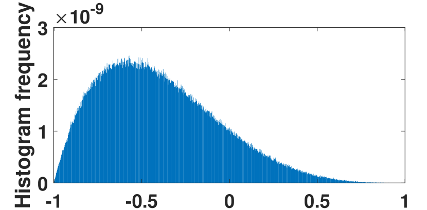
(a) Beta(2,5), O=-0.3994.

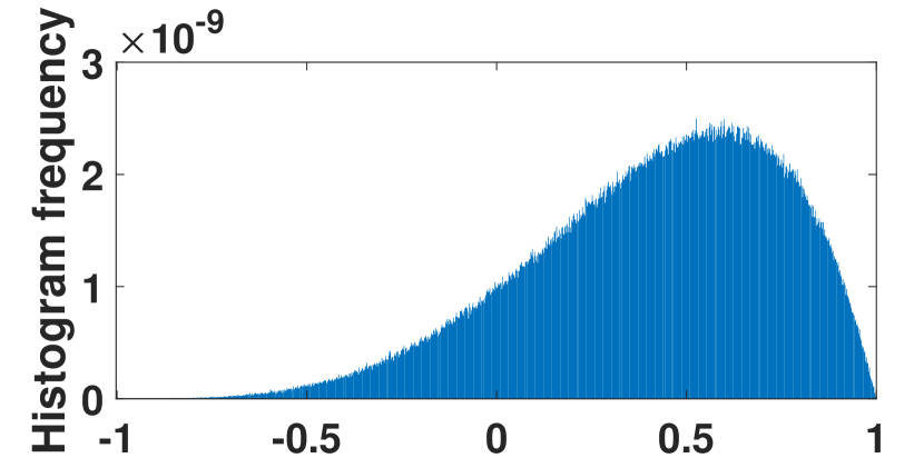
(b) Beta(5,2), O=0.4136.

(c) Taxi, O=0.1190.

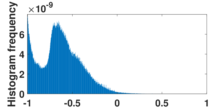
(d) Retirement, O=-0.6240.

Figure 4: Normalized frequencies of datasets

In this section, we evaluate the performance of both EMF and DAP, on both real-world and synthetic datasets. The source code and datasets are available in [17].

VI-A Experiment Setup

Datasets. We adopt two synthetic and two real-world numerical datasets. Beta(2,5) and Beta(5,2) are two synthetic datasets drawn from Beta distribution [32], each with 1,000,000 samples in the interval $[0,1]$. Taxi [49] is the pick-up time in a day extracted from 2018 January New York Taxi data, which contains 1,048,575 integers from 0 to 86,340 (the number of seconds in 24 hours). Retirement [23] is extracted from the San Francisco employee retirement plans, which contains the salary and benefits paid to city employees since fiscal year 2013. We employ the total compensation, which comprises a subset of 606,507 items in the interval $[10000,60000]$. All these datasets are then normalized into interval $[-1,1]$. The normalized frequency histograms of all datasets are plotted in Fig. 4.

Parameters Setting. We use PM as our default perturbation mechanism, and set the right side as the default poisoned side. Therefore, the poison values are injected into poison values’ range $[r_{l},r_{r}]\subset[O,C]$, denoted by $Poi_{[r,l]}$ in the figures. To evaluate the scalability of our protocol, we apply our schemes with different parameters, including poison values’ ranges and poison value distributions. We set a series of $r_{l}<r_{r}$ for different poison values’ ranges. When the poisoned side is estimated as the right-hand one by Algorithm 3, we set the probing range to $[O^{\prime},C]$ (resp. $[-C,O^{\prime}]$ if the side is to the left). The proportion of Byzantine users is set to 25% and the poison values are uniformly distributed in $[r_{l},r_{r}]$ by default. The termination condition for EMF/EMF*/CEMF* is $|l(F)^{t}-l(F)^{t+1}|<\tau$, where $\tau$ is set to $0.01e^{\epsilon}$. We choose $d^{\prime}=\lfloor\sqrt{N}\rfloor$ and $d=\lfloor\frac{d^{\prime}(e^{\epsilon/2}-1)}{e^{\epsilon/2}+1}\rfloor$.

VI-B Effectiveness of EMF

TABLE I: Variance of reconstructed normal data

$Poi_{[l,r]}$	Side	Privacy budget $\epsilon$
		2	0.5	0.25	0.125	0.0625
$[\frac{3}{4}C,C]$	L	3.8E-03	1.4E-03	2.7E-03	2.7E-03	1.5E-03
	R	2.0E-07	4.9E-06	1.1E-05	1.6E-05	1.9E-05
$[\frac{1}{2}C,C]$	L	1.4E-04	5.7E-04	1.1E-03	1.0E-03	7.0E-04
	R	4.1E-07	4.2E-06	9.0E-06	1.3E-05	1.4E-05
$[O,\frac{1}{2}C]$	L	7.6E-06	1.7E-05	3.4E-05	4.3E-05	4.1E-05
	R	3.0E-07	3.9E-06	8.4E-06	1.2E-05	1.3E-05
$[O,C]$	L	1.3E-05	1.8E-04	4.3E-04	5.0E-04	4.4E-04
	R	2.7E-07	3.1E-06	5.8E-06	7.4E-06	7.9E-06

Poisoned Side Estimation. We conduct experiments on both sides to evaluate the effectiveness of Algorithm 3 that determines the poisoned side. We can see from results on Taxi shown in Table I that EMF on the right side always has a smaller variance under different privacy budgets and poison values’ ranges. Based on this, Algorithm 3 can determine the correct poisoned side, which is the right side with smaller variance. The correct estimation is attributed to two reasons. On one hand, $\hat{x}$ of the correct side can have a lower variance than the incorrect side, which is proved in Theorem 3. On the other hand, even if the wrong side is initially chosen, all poison values will be assigned to the non-poisoned side and cause a surge in the right of the distribution for normal users, which will also lead to a larger variance.

Proportion of Byzantine Users. In the first set of experiments, we verify the accuracy of the proportion of Byzantine users obtained by EMF w.r.t. $\epsilon$ in Fig. 5.

Given a fixed privacy budget, we compare the four poison values’ ranges $[3C/4,C],[C/2,C],[O,C/2]$ and $[O,C]$ in Fig. 5 (a) (b). When $\epsilon$ is large, the estimated proportion deviates from the real proportion of Byzantine users $\gamma$. As $\epsilon$ decreases, the result becomes more accurate. The reason is that according to Theorem 3, when $\epsilon$ becomes smaller, EMF distinguishes normal and poison values better. In these figures, regardless of poison values’ ranges, datasets and $\gamma$, $|\hat{\gamma}-\gamma|$ converges to 0 as $\epsilon\rightarrow 0$. This shows the robustness of EMF even under adverse conditions where many normal values are mistreated as poison values.

Fig. 5 (c) evaluates $\hat{\gamma}$ when there is no poison value in the system, and the proportion of Byzantine users estimated by EMF is equivalent to the false positive rate ($fpr$). When $\epsilon_{0}$ gets smaller, $fpr$ becomes less relevant to normal users’ distribution. According to Theorem 3, the smaller $\epsilon_{0}$ is, the more accurate the estimated proportion of Byzantine users becomes. We observe for all 4 datasets and $\epsilon_{0}=\frac{1}{16}$, and the false positives range from 0.02 to 0.04, which are quite small. In Fig. 5 (d), we evaluate $\hat{\gamma}$ when Byzantine users inject their poison values as 1 and then perturb as normal users, which is also known as an input manipulation attack (IMA) [38]. We observe that $\hat{\gamma}$ is between $0.03\sim 0.04$, which means EMF cannot filter out these Byzantine users due to the perturbation. Nonetheless, we can further enhance the utility with existing detection techniques (such as k-means clustering [38]), which will be shown in Fig.9 (b).

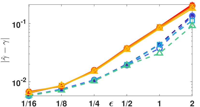
(a) $\gamma=0.1$.

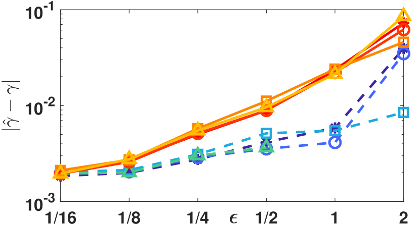
(b) $\gamma=0.4$.

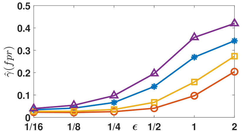
(c) $\gamma=0$.

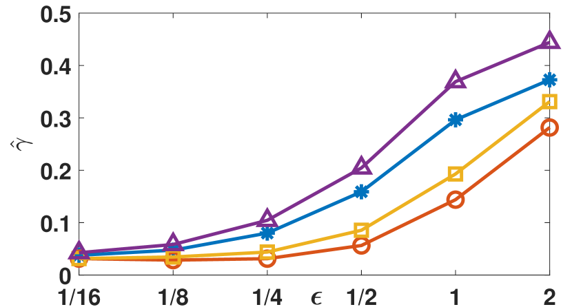
(d) IMA, $\gamma=0.25$.

Figure 5: The proportion of Byzantine users estimated by EMF w.r.t. $\epsilon$

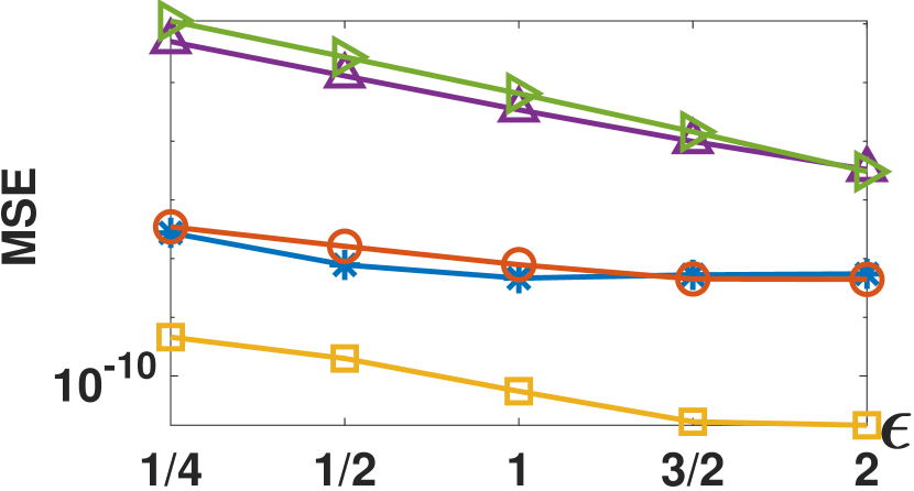
(a) Beta(2,5), $Poi_{[3C/4,C]}$.

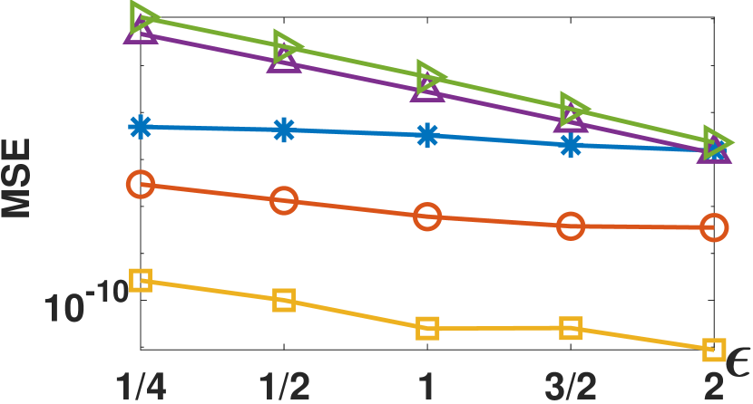
(b) Beta(5,2), $Poi_{[3C/4,C]}$.

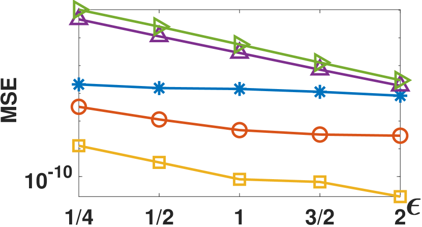
(c) Taxi, $Poi_{[3C/4,C]}$.

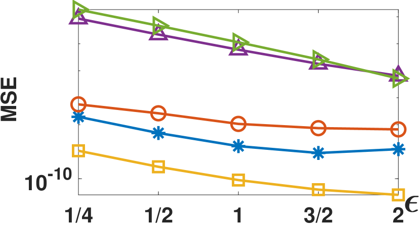
(d) Retirement, $Poi_{[3C/4,C]}$.

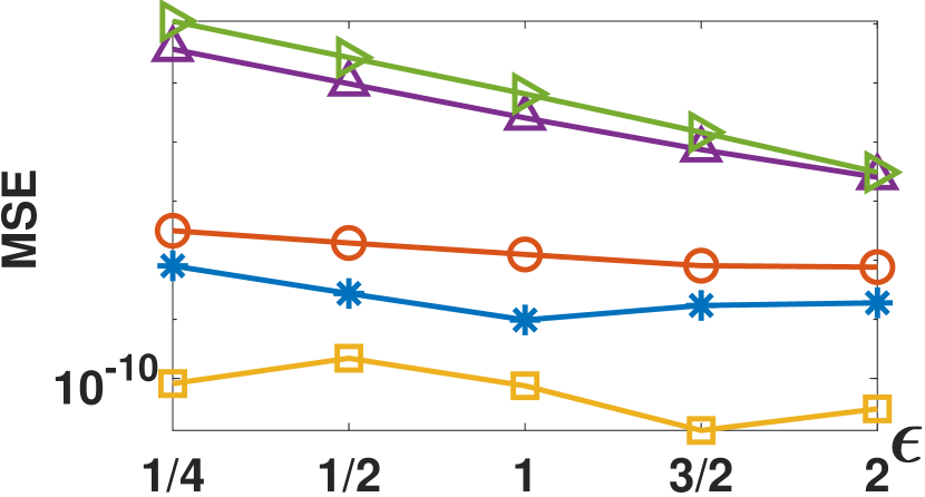
(e) Beta(2,5), $Poi_{[1C/2,C]}$.

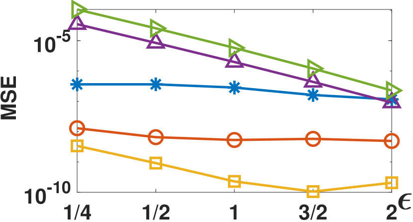
(f) Beta(5,2), $Poi_{[1C/2,C]}$.

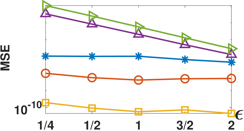
(g) Taxi, $Poi_{[1C/2,C]}$.

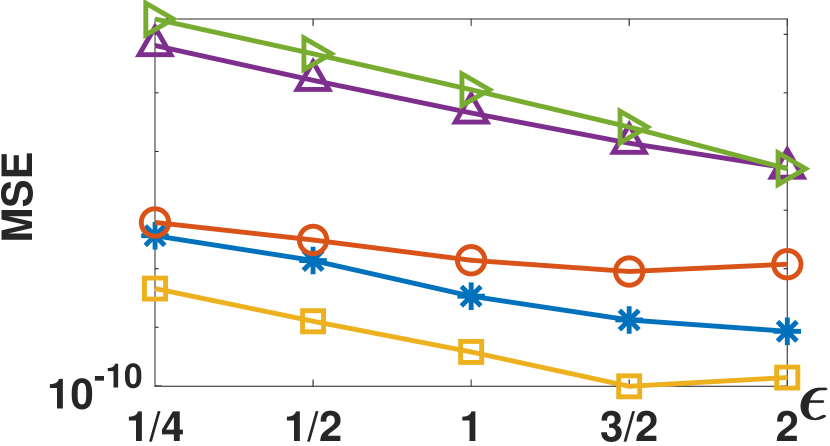
(h) Retirement, $Poi_{[1C/2,C]}$.

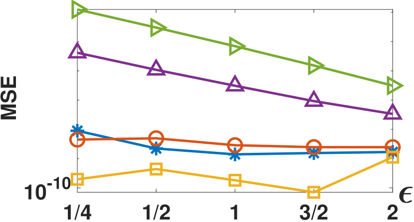
(i) Beta(2,5), $Poi_{[O,1C/2]}$.

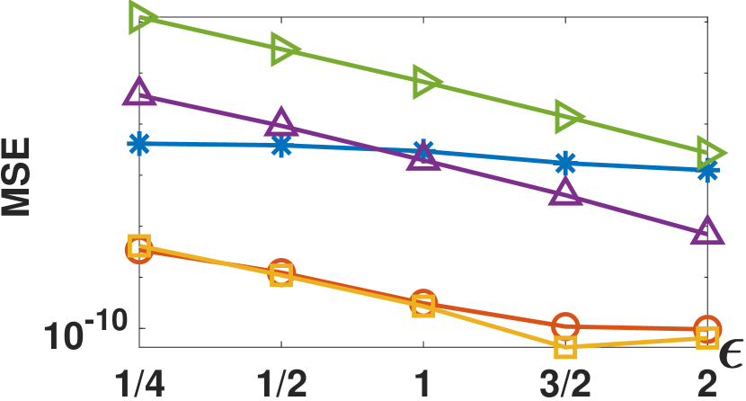
(j) Beta(5,2), $Poi_{[O,1C/2]}$.

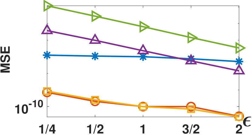
(k) Taxi, $Poi_{[O,1C/2]}$.

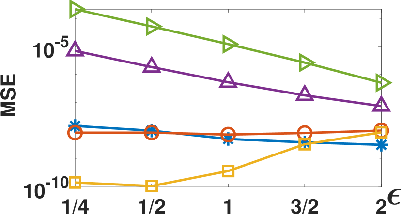
(l) Retirement, $Poi_{[O,1C/2]}$.

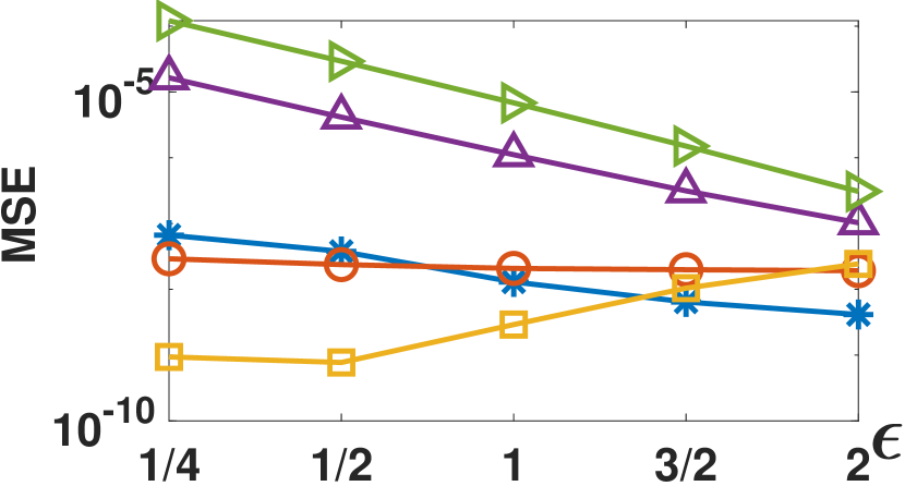
(m) Beta(2,5), $Poi_{[O,C]}$.

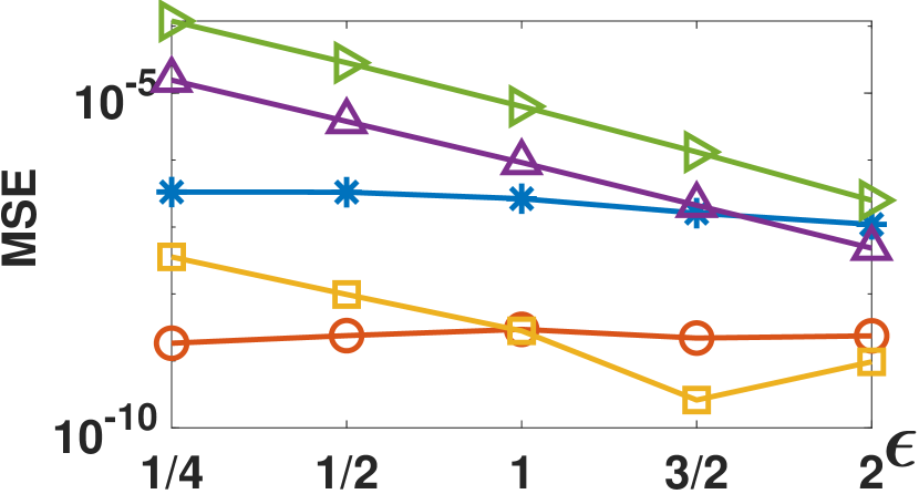
(n) Beta(5,2), $Poi_{[O,C]}$.

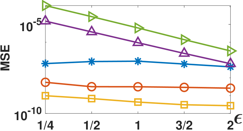
(o) Taxi, $Poi_{[O,C]}$.

(p) Retirement, $Poi_{[O,C]}$.

Figure 6: MSE on mean estimation w.r.t. $\epsilon$

VI-C Performance of DAP

Mean Estimation. Fig. 6 compares the MSE [46] of mean estimation among five schemes, including $DAP_{EMF}$, $DAP_{EMF^{*}}$, $DAP_{CEMF^{*}}$, Ostrich, and Trimming. Ostrich is the baseline method where all values are directly averaged and the existence of Byzantine users is ignored. For Trimming, the data collector simply removes the largest (or smallest if the poison side is to the left) 50% values in $V^{\prime}$ and averages the remaining values.

EMF, EMF*, and CEMF* estimations are used in three DAP schemes, known as $DAP_{EMF}$, $DAP_{EMF^{*}}$, and $DAP_{CEMF^{*}}$, respectively. Note that the latter two are post-processing of EMF, so essentially they mean EMF+EMF* and EMF+CEMF*. In the DAP protocol, the minimum privacy budget $\epsilon_{0}$ in all groups is set to 1/16, and $\epsilon$ is set to $\{1/4,1/2,1,3/2,2\}$. The lower threshold of $DAP_{CEMF^{*}}$ to suppress buckets is set to $0.5\hat{\gamma}/(d^{\prime}/2)$.

In Fig. 6, in most cases Trimming underperforms others as it overkills many normal values. Furthermore, all proposed schemes outperform Ostrich and Trimming, as they more or less manage to probe some poison values. Among the three schemes we propose, $DAP_{EMF^{*}}$ performs better than $DAP_{EMF}$ in most cases because $DAP_{EMF}$ may remove an inappropriate number of values, which is resolved by $DAP_{EMF^{*}}$. In most cases, $DAP_{CEMF^{*}}$ behaves better than $DAP_{EMF^{*}}$, as the former further suppresses some buckets unchosen by Byzantine users and therefore has a smaller error on the convergence result. In Figs. 6 (j) (k) (n), we observe that EMF performs worse than the Ostrich scheme when $\epsilon$ is large in Beta(5,2) and Taxi. This is because the poison values are coincidentally close to the true mean value $O$, while EMF probes too many poison values and incorrectly removes some normal values.

In Figs. 6 (l) (m) (p), we observe that the MSE of $DAP_{CEMF^{*}}$ decreases with increasing $\epsilon$, because EMF tends to overestimate poison values when $\epsilon$ and the poison values’ range are large. Therefore, CEMF* is less likely to suppress buckets without poison values, which degrades the utility. Nonetheless, $DAP_{CEMF^{*}}$ is still better than most other schemes. As a final note, since empirically EMF* probes poison values better than EMF, $DAP_{EMF*}$ is expected to outperform $DAP_{EMF}$. However, it contradicts with the results in Fig. 6 (d) (e) (h). We attribute this phenomenon to false positives, which are misjudge values that should have contributed to mean estimation as normal users. Nonetheless, the performance gap between $DAP_{EMF*}$ and $DAP_{EMF}$ is not significant.

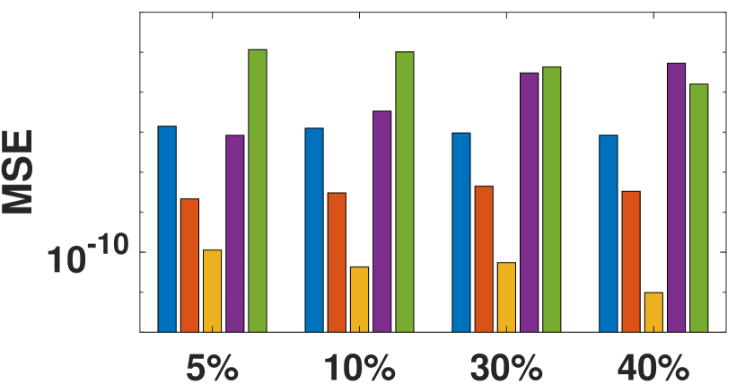
(a) Taxi, $Poi_{[O,C/2]}$.

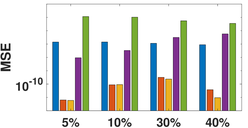
(b) Taxi, $Poi_{[C/2,C]}$.

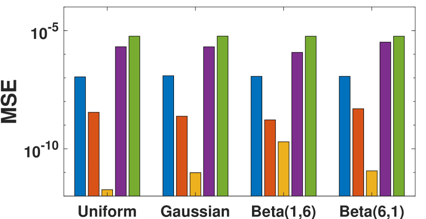
(c) Taxi, $Poi_{[O,C/2]}$.

(d) Taxi, $Poi_{[C/2,C]}$.

Figure 7: The results of MSE w.r.t. $\gamma$ for (a) (b) and w.r.t. the distribution of Byzantine users for (c) (d)

Robustness of Poison Values. Fig. 7 shows the robustness of MSE according to different proportions of Byzantine users and distributions of poison values in Taxi at $\epsilon=1$. Fig. 7 (a) (b) show that, even with increasing Byzantine users ($\gamma$ reaches 40%), our proposed schemes can still achieve very low MSE. Fig. 7 (c) (d) show the MSE varies w.r.t. different distributions of poison values. We can find the performance varies according to what the distribution of poison values is, and the proposed schemes always outperform others. In Figs. 7 (a) (b) (d), Ostrcih behaves better than $DAP_{EMF}$ in some cases, when the proportion of Byzantine users is small and the poison values are close to $O$. In Fig. 7 (d), when the poison values follows Gaussian distribution, $DAP_{EMF^{*}}$ outperforms $DAP_{CEMF^{*}}$, because the latter may wrongly suppress some buckets and introduce more errors. To sum up, the proposed schemes consistently outperform others under various proportions of Byzantine users or the distributions of poison values.

VI-D Generalizability Analysis

Extension to Distribution Estimation and SW Mechanism. Fig. 8 (a) evaluates the distribution estimation accuracy by using the Wasserstein distance[39]. The results demonstrate that our schemes achieve at least 10% higher utility than Ostrich, which ignores the presence of poison values, whereas our schemes can still refine the distribution by removing them. Figs. 8(b)-(d) evaluate the DAP performance on SW. Fig. 8 (b) shows that the estimated proportion of Byzantine users becomes more accurate as $\epsilon$ decreases. In Figs. 8 (c) (d), we compare the MSE of different schemes with poison values’ range $[1+b/2,1+b]$, and observe that our proposed schemes outperform the others in most cases. Specifically, Trimming and Ostrich only perform well for small $\epsilon$ on Beta(2,5) and Beta(5,2), respectively. This is because when $\epsilon$ is small, the perturbed values are close to a uniform distribution, so the estimated mean tends to be 0.5. But Trimming will estimate a smaller mean as it removes large values, while Ostrich may accidentally admit some large values, making the estimated mean closer to the ground truth.

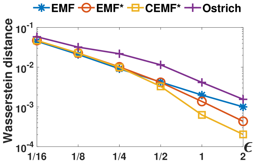
(a) Beta(2,5), O=0.3003.

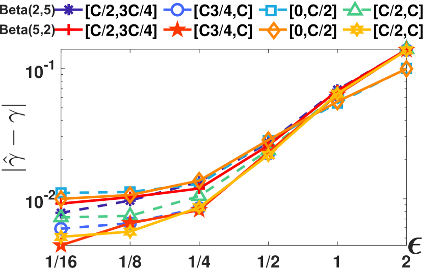
(b) Beta(5,2), O=0.7068.

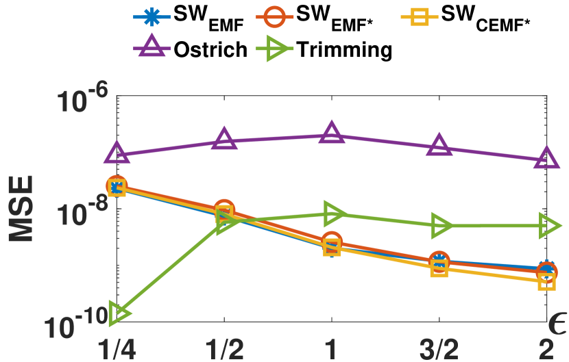
(c) Beta(2,5), O=0.3003.

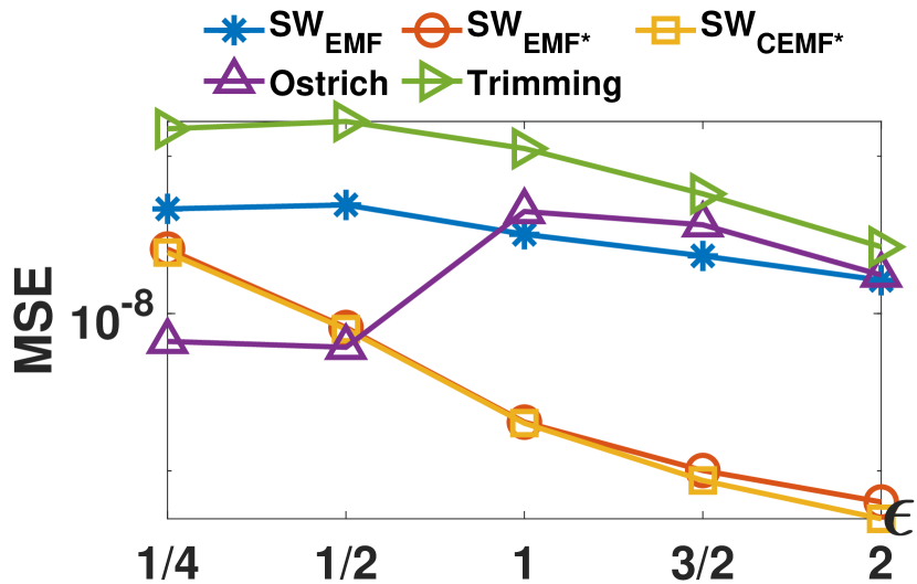
(d) Beta(5,2), O=0.7068.

Figure 8: The results of distribution estimation for (a), SW w.r.t. $\epsilon$, $|\hat{\gamma}-\gamma|$ for (b) and MSE for (c) (d)

Comparison with k-means-based Defense. We compare our solution with the k-means-based defense [38] against both BBA and input manipulation attacks on Taxi. K-means-based defense samples multiple subsets of users and then clusters them into two clusters. The one with more subsets is treated as normal users and used for estimation, while the other is discarded. Let $\beta$ be the sampling rate, and $\beta N$ users are sampled randomly in each subset, with one million subsets in each attack.

In Fig. 9 (a), the poison values are distributed on $[C/2,C]$ uniformly, and our scheme outperforms the k-means-based defense under BBA attack. The MSE of the k-means family is between $10^{-7}\sim 10^{-5}$, whereas the MSE of $DAP_{EMF}$ is about $10^{-7}$ and that of $DAP_{EMF^{*}}$ and $DAP_{CEMF^{*}}$ is about $10^{-10}$. Fig. 9 (b) evaluates the input manipulation attack [12] based on PM, i.e., Byzantine users generating an input poison value $g$ and then strictly following PM to make it less detectable. To integrate EMF and EMF* with existing k-means-based defense, we first use EMF to determine whether $\hat{\gamma}$ is relatively small (i.e., evading) as shown in Fig. 5 (d), and then we use EMF* to estimate the distribution of inputs by setting $\hat{\gamma}=0$ in Equ. 6, and finally we evaluate the mean using k-means. Fig. 9 (b) demonstrates that by such integration (denoted by EMF-based), we can further improve the estimation accuracy under input manipulation attacks. When $g=-1$, the MSE of EMF-based is between $1.40\sim 1.44\times 10^{-7}$ while that of k-means alone is between $1.77\sim 1.88\times 10^{-7}$, resulted in 28% improvement. Likewise, we have about 30% improvement for $g=1$ and $g=0$ cases.

Frequency Estimation on Categorical Data. We evaluate our schemes under frequency estimation on categorical data using dataset COVID-19, which records the number of coronavirus disease 2019 deaths for females in California as of December 14, 2022, by age [61]. All death records are divided into $15$ age groups, and every record is perturbed locally by k-RR [33, 63]. In Fig. 9 (c), Byzantine users are injected into the 10th group only, and we observe that the MSE of Ostrich is about 0.1 and keeps steady regardless of $\epsilon$, while that of our schemes is lower than 0.01 and decreases significantly with respect to $\epsilon$. When Byzantine users uniformly inject poison values into the 10th, 11th, and 12th groups, as shown in Fig. 9 (d), the MSE of Ostrich still significantly underperforms our schemes. This experiment shows that our DAP schemes can also work well in other statistics and data types than mean estimation on numerical data.

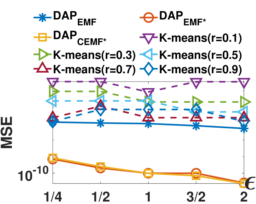
(a) Taxi, $Poi_{[C/2,C]}$, $\gamma=0.25$.

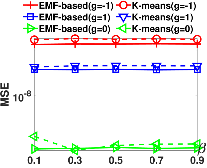
(b) Taxi, IMA, $\gamma=0.25$.

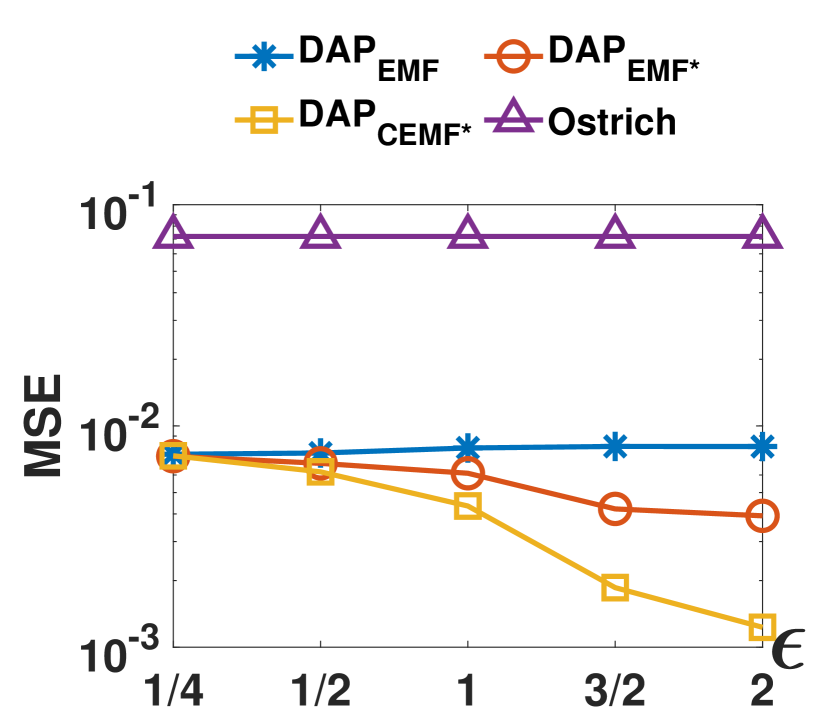
(c) COVID-19, $Poi_{10}$.

(d) COVID-19, $Poi_{10,11,12}$.

Figure 9: Comparison with k-means-based defense for (a) (b) and extension to frequency estimation for (c) (d)

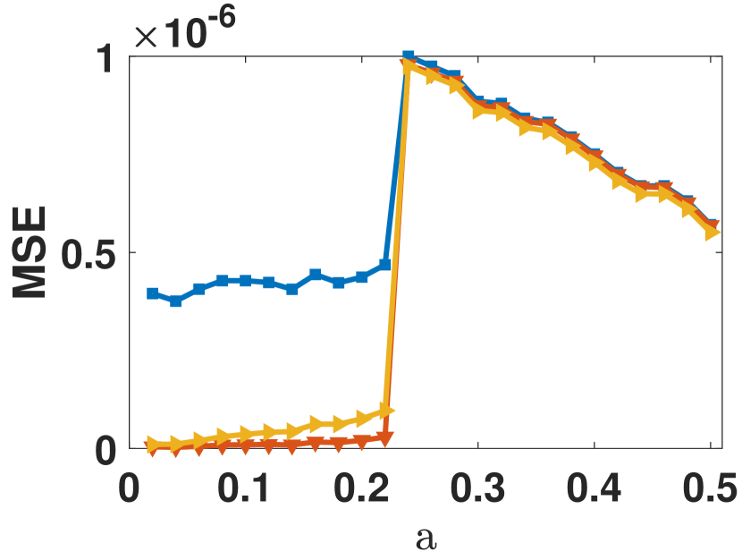
(a) Beta(2,5), $O=0.4136$.

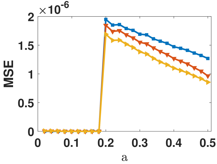
(b) Beta(5,2), $O=-0.3994$.

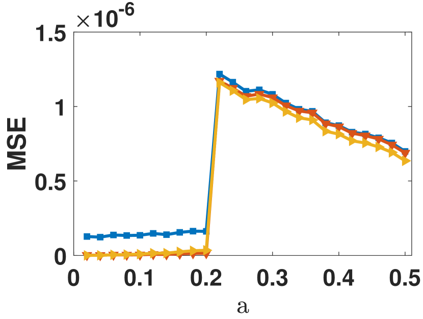
(c) Taxi, $O=0.1190$.

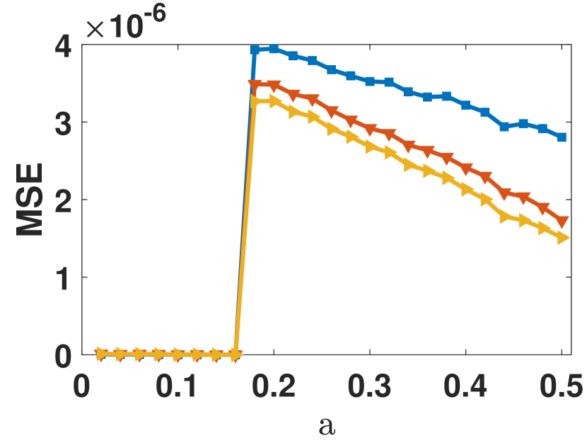
(d) Taxi, $O=-0.6240$.

Figure 10: The results of MSE w.r.t. $a$

Robustness of Evasion. We test the evasion effect on four datasets where $\epsilon=1/2$ and $\gamma=0.25$. A total of $m$ Byzantine users inject $am$ evasive poison values at $-C/2$ (where $-C/2<O^{\prime}$) and $(1-a)m$ true poison values uniformly on $[C/2,C]$, where $a$ is the percentage of evasive poison values. In Fig. 10, we plot the MSE of mean estimation, which essentially measures the utility of poison values. We observe that when $a$ is small, all DAPs still work well and ignore the evasive poison values. When $a$ is larger than a threshold (around 20%–30%), the MSE suddenly goes up high, because these evasive poison values finally become effective, and our schemes begin to misjudge the poisoned side. After that, the MSE starts to drop, which means such evasion will lose effectiveness as there are fewer true poison values.

VII Related Work

Local differential privacy (LDP) [11, 19, 34], a variant of DP [21, 22, 45], is proposed to protect the data privacy of users in an untrusted environment. RAPPOR [24], an extension deployed within Chrome by Google, was the first client-based practical privacy solution. After that, the LDP technique has been widely applied in the industry to protect their users’ privacy, like iOS for Apple [60] Win 10 for Microsoft [14], and Samsung [47]. Since the concept of LDP was proposed, it has been widely applied in multiple fields, including multi-attribute values estimation [53, 18] marginal release [13, 73], time series data release [69], graph data collection [59, 68, 67], key-value data collection [70, 28, 71] and private learning [74, 75].

Mean and frequency estimations are commonly seen in LDP scenarios. Several mechanisms [1, 4, 5, 14, 24, 64, 39] are proposed for frequency estimation under LDP. Among them, the most relevant work to estimate numerical data by using EM algorithm in LDP is the SW mechanism  [39]. However, the SW mechanism is not designed for combating Byzantine attacks, and is therefore unable to eliminate the impact of poison values. For mean estimation, Duchi et. al propose a 1-bit mechanism [20] and Wang et. al [62] propose the Piecewise Mechanism are the state of the art methods for mean estimation.

The problems of the Byzantine attacks, that is, data poisoning attacks have recently been studied in many fields, such as crowdsourcing and crowdsensing scenarios [10, 27], applications of Internet of Things [31, 54], electric power grids [42] and machine learning algorithms [8, 25, 26]. However, combating Byzantine attacks in LDP protocols is a relatively new topic that has few state-of-the-art papers. Literature [12] figures out that LDP is vulnerable to manipulation attacks. With a small privacy budget or a large input domain, a few poisoned values can completely ruin the real distribution. To combat this kind of attack, sampling is an easy but effective approach. Literature [7] formulates the data poisoning attack as an optimization problem and proposes three attacking patterns to maximize their attacking effectiveness, and design some countermeasures accordingly. Literature [65] is the first attempt at poisoning attacks for key-value data in LDP protocols. They formulate an attack with two objectives, which are to simultaneously maximize the frequencies and mean values and to design two countermeasures against this attack. Literature [35] proposes a novel verifiable LDP protocol based on Multi-Party Computation (MPC) techniques. They propose a verifiable randomization mechanism in which the data collector can verify the completeness of executing an agreed randomization mechanism for every data provider. However, this method is only proposed for the categorical frequency oracles, such as kRR [33], OUE [64] and OLH [64] instead of mean and distribution estimation on numerical values.

VIII Conclusion

This paper address the general Byzantine attacks in LDP mechanisms, which advances state-of-the-art works by eliminating prior knowledge of either the attacking pattern or the poison value distribution. We present EMF, a novel algorithm to estimate key Byzantine users’ features, including the proportion of Byzantine users and the poisoned side, which are then utilized to improve the mean estimation accuracy. To further enhance the utility and security of our scheme, we propose a group-wise protocol DAP and two post-processing schemes (EMF* and CEMF*) of EMF that collectively achieves the optimized mean value in terms of variance. Extensive empirical studies verify the correctness and effectiveness of the DAP protocol.

References

- [1] Jayadev Acharya, Ziteng Sun, and Huanyu Zhang. Hadamard response: Estimating distributions privately, efficiently, and with little communication. In The 22nd International Conference on Artificial Intelligence and Statistics, pages 1120–1129. PMLR, 2019.
- [2] P Arthur. Maximum likelihood from incomplete data via the em algorithm. Journal of The Royal Statistical Society Series B, 39(1):1–38, 1977.
- [3] Baruch Awerbuch, Reza Curtmola, David Holmer, Cristina Nita-Rotaru, and Herbert Rubens. Mitigating byzantine attacks in ad hoc wireless networks. Department of Computer Science, Johns Hopkins University, Tech. Rep. Version, 1:16, 2004.
- [4] Raef Bassily, Kobbi Nissim, Uri Stemmer, and Abhradeep Guha Thakurta. Practical locally private heavy hitters. In Advances in Neural Information Processing Systems, pages 2288–2296, 2017.
- [5] Raef Bassily and Adam Smith. Local, private, efficient protocols for succinct histograms. In Proceedings of the forty-seventh annual ACM symposium on Theory of computing, pages 127–135, 2015.
- [6] Jeff A Bilmes et al. A gentle tutorial of the em algorithm and its application to parameter estimation for gaussian mixture and hidden markov models. International Computer Science Institute, 4(510):126, 1998.
- [7] Xiaoyu Cao, Jinyuan Jia, and Neil Zhenqiang Gong. Data poisoning attacks to local differential privacy protocols. In 30th USENIX Security Symposium (USENIX Security 21), 2021.
- [8] Nicholas Carlini. Poisoning the unlabeled dataset of Semi-Supervised learning. In 30th USENIX Security Symposium (USENIX Security 21), pages 1577–1592, 2021.
- [9] Andrea Cerioli, Alessio Farcomeni, and Marco Riani. Wild adaptive trimming for robust estimation and cluster analysis. Scandinavian Journal of Statistics, 46(1):235–256, 2019.
- [10] Shih-Hao Chang and Zhi-Rong Chen. Protecting mobile crowd sensing against sybil attacks using cloud based trust management system. Mobile Information Systems, 2016, 2016.
- [11] Rui Chen, Haoran Li, A Kai Qin, Shiva Prasad Kasiviswanathan, and Hongxia Jin. Private spatial data aggregation in the local setting. In 2016 IEEE 32nd International Conference on Data Engineering (ICDE), pages 289–300. IEEE, 2016.
- [12] Albert Cheu, Adam Smith, and Jonathan Ullman. Manipulation attacks in local differential privacy. In 2021 IEEE Symposium on Security and Privacy (SP), pages 883–900. IEEE, 2021.
- [13] G. Cormode, T. Kulkarni, and D. Srivastava. Marginal release under local differential privacy. In SIGMOD, pages 131–146. ACM, 2018.
- [14] Bolin Ding, Janardhan Kulkarni, and Sergey Yekhanin. Collecting telemetry data privately. arXiv preprint arXiv:1712.01524, 2017.
- [15] Zhiguo Ding and Minrui Fei. An anomaly detection approach based on isolation forest algorithm for streaming data using sliding window. IFAC Proceedings Volumes, 46(20):12–17, 2013.
- [16] Wilfrid J Dixon and Kareb K Yuen. Trimming and winsorization: A review. Statistische Hefte, 15(2):157–170, 1974.
- [17] Rong Du. The source code for differential aggregation protocol. https://github.com/RONGDUGithub/DAP, 2023.
- [18] Rong Du, Qingqing Ye, Yue Fu, and Haibo Hu. Collecting high-dimensional and correlation-constrained data with local differential privacy. In 2021 18th Annual IEEE International Conference on Sensing, Communication, and Networking (SECON), pages 1–9. IEEE, 2021.
- [19] John C Duchi, Michael I Jordan, and Martin J Wainwright. Local privacy and statistical minimax rates. In 2013 IEEE 54th Annual Symposium on Foundations of Computer Science, pages 429–438. IEEE, 2013.
- [20] John C Duchi, Michael I Jordan, and Martin J Wainwright. Minimax optimal procedures for locally private estimation. Journal of the American Statistical Association, 113(521):182–201, 2018.
- [21] Cynthia Dwork. Differential privacy: A survey of results. In International conference on theory and applications of models of computation, pages 1–19. Springer, 2008.
- [22] Cynthia Dwork, Frank McSherry, Kobbi Nissim, and Adam Smith. Calibrating noise to sensitivity in private data analysis. In Theory of cryptography conference, pages 265–284. Springer, 2006.
- [23] The San Francisco employee retirement plans in 2013. Retirement dataset. https://www.kaggle.com/datasets/san-francisco/sf-employee-compensation, 2013.
- [24] Úlfar Erlingsson, Vasyl Pihur, and Aleksandra Korolova. Rappor: Randomized aggregatable privacy-preserving ordinal response. In Proceedings of the 2014 ACM SIGSAC conference on computer and communications security, pages 1054–1067, 2014.
- [25] Minghong Fang, Xiaoyu Cao, Jinyuan Jia, and Neil Gong. Local model poisoning attacks to Byzantine-Robust federated learning. In 29th USENIX Security Symposium (USENIX Security 20), pages 1605–1622, 2020.
- [26] Minghong Fang, Neil Zhenqiang Gong, and Jia Liu. Influence function based data poisoning attacks to top-n recommender systems. In Proceedings of The Web Conference 2020, pages 3019–3025, 2020.
- [27] Ujwal Gadiraju, Ricardo Kawase, Stefan Dietze, and Gianluca Demartini. Understanding malicious behavior in crowdsourcing platforms: The case of online surveys. In Proceedings of the 33rd Annual ACM Conference on Human Factors in Computing Systems, pages 1631–1640, 2015.
- [28] Xiaolan Gu, Ming Li, Yueqiang Cheng, Li Xiong, and Yang Cao. PCKV: locally differentially private correlated key-value data collection with optimized utility. In USENIX Security Symposium, 2020.
- [29] Liang Hu, Longbing Cao, Jian Cao, Zhiping Gu, Guandong Xu, and Jie Wang. Improving the quality of recommendations for users and items in the tail of distribution. ACM Transactions on Information Systems (TOIS), 35(3):1–37, 2017.
- [30] Nan Hu, Ling Liu, and Vallabh Sambamurthy. Fraud detection in online consumer reviews. Decision Support Systems, 50(3):614–626, 2011.
- [31] Vittorio P Illiano and Emil C Lupu. Detecting malicious data injections in wireless sensor networks: A survey. ACM Computing Surveys (CSUR), 48(2):1–33, 2015.
- [32] Norman L Johnson, Samuel Kotz, and Narayanaswamy Balakrishnan. Continuous univariate distributions, volume 2, volume 289. John wiley & sons, 1995.
- [33] Peter Kairouz, Sewoong Oh, and Pramod Viswanath. Extremal mechanisms for local differential privacy. In Advances in neural information processing systems, pages 2879–2887, 2014.
- [34] Shiva Prasad Kasiviswanathan, Homin K Lee, Kobbi Nissim, Sofya Raskhodnikova, and Adam Smith. What can we learn privately? SIAM Journal on Computing, 40(3):793–826, 2011.
- [35] Fumiyuki Kato, Yang Cao, and Masatoshi Yoshikawa. Preventing manipulation attack in local differential privacy using verifiable randomization mechanism. arXiv preprint arXiv:2104.06569, 2021.
- [36] Husheng Li and Zhu Han. Catching attacker (s) for collaborative spectrum sensing in cognitive radio systems: An abnormality detection approach. In 2010 IEEE Symposium on New Frontiers in Dynamic Spectrum (DySPAN), pages 1–12. IEEE, 2010.
- [37] Ninghui Li, Min Lyu, Dong Su, and Weining Yang. Differential privacy: From theory to practice. Synthesis Lectures on Information Security, Privacy, & Trust, 8(4):1–138, 2016.
- [38] Xiaoguang Li, Neil Zhenqiang Gong, Ninghui Li, Wenhai Sun, and Hui Li. Fine-grained poisoning attacks to local differential privacy protocols for mean and variance estimation. arXiv preprint arXiv:2205.11782, 2022.
- [39] Zitao Li, Tianhao Wang, Milan Lopuhaä-Zwakenberg, Ninghui Li, and Boris Škoric. Estimating numerical distributions under local differential privacy. In Proceedings of the 2020 ACM SIGMOD International Conference on Management of Data, pages 621–635, 2020.
- [40] Fang Liu, Xiuzhen Cheng, and Dechang Chen. Insider attacker detection in wireless sensor networks. In IEEE INFOCOM 2007-26th IEEE International Conference on Computer Communications, pages 1937–1945. IEEE, 2007.
- [41] Fei Tony Liu, Kai Ming Ting, and Zhi-Hua Zhou. Isolation forest. In 2008 eighth ieee international conference on data mining, pages 413–422. IEEE, 2008.
- [42] Yao Liu, Peng Ning, and Michael K Reiter. False data injection attacks against state estimation in electric power grids. ACM Transactions on Information and System Security (TISSEC), 14(1):1–33, 2011.
- [43] Michael Luca and Georgios Zervas. Fake it till you make it: Reputation, competition, and yelp review fraud. Management Science, 62(12):3412–3427, 2016.
- [44] Dina Mayzlin, Yaniv Dover, and Judith Chevalier. Promotional reviews: An empirical investigation of online review manipulation. American Economic Review, 104(8):2421–55, 2014.
- [45] Frank McSherry and Kunal Talwar. Mechanism design via differential privacy. In 48th Annual IEEE Symposium on Foundations of Computer Science (FOCS’07), pages 94–103. IEEE, 2007.
- [46] Mc Farlane Mood. Introduction to the theory of statistics. McGraw-Hill, 1963.
- [47] Thông T Nguyên, Xiaokui Xiao, Yin Yang, Siu Cheung Hui, Hyejin Shin, and Junbum Shin. Collecting and analyzing data from smart device users with local differential privacy. arXiv preprint arXiv:1606.05053, 2016.
- [48] David J Olive. Applied robust statistics. Preprint M-02-006, 2008.
- [49] The pick-up time in a day extracted from 2018 January New York Taxi data. Taxi dataset. https://www.kaggle.com/code/wti200/exploratory-analysis-nyc-taxi-trip, 2018.
- [50] Saurav Prakash and Amir Salman Avestimehr. Mitigating byzantine attacks in federated learning. arXiv preprint arXiv:2010.07541, 2020.
- [51] Ankit Singh Rawat, Priyank Anand, Hao Chen, and Pramod K Varshney. Collaborative spectrum sensing in the presence of byzantine attacks in cognitive radio networks. IEEE Transactions on Signal Processing, 59(2):774–786, 2010.
- [52] Ankit Singh Rawat, Priyank Anand, Hao Chen, and Pramod K Varshney. Countering byzantine attacks in cognitive radio networks. In 2010 IEEE International Conference on Acoustics, Speech and Signal Processing, pages 3098–3101. IEEE, 2010.
- [53] Xuebin Ren, Chia-Mu Yu, Weiren Yu, Shusen Yang, Xinyu Yang, Julie A McCann, and S Yu Philip. Lopub: High-dimensional crowdsourced data publication with local differential privacy. IEEE Transactions on Information Forensics and Security, 13(9):2151–2166, 2018.
- [54] Mohsen Rezvani, Aleksandar Ignjatovic, Elisa Bertino, and Sanjay Jha. Secure data aggregation technique for wireless sensor networks in the presence of collusion attacks. IEEE transactions on Dependable and Secure Computing, 12(1):98–110, 2014.
- [55] Dwijen Rudrapal, Smita Das, Nikhil Debbarma, and Swapan Debbarma. Internal attacker detection by analyzing user keystroke credential. Lecture Notes on Software Engineering, 1(1):49, 2013.
- [56] Neil C Schwertman, Margaret Ann Owens, and Robiah Adnan. A simple more general boxplot method for identifying outliers. Computational statistics & data analysis, 47(1):165–174, 2004.
- [57] Huasong Shan, Qingyang Wang, and Calton Pu. Tail attacks on web applications. In Proceedings of the 2017 ACM SIGSAC Conference on Computer and Communications Security, pages 1725–1739, 2017.
- [58] P Street, N Haven, and D Mayzlin. Promotional chat on the internet. 25 (2), 155-163, 2006.
- [59] Haipei Sun, Xiaokui Xiao, Issa Khalil, Yin Yang, Zhan Qin, Hui Wendy Wang, and Ting Yu. Analyzing subgraph statistics from extended local views with decentralized differential privacy. In CCS, pages 703–717. ACM, 2019.
- [60] ADP Team et al. Learning with privacy at scale. Apple Mach. Learn. J, 1(8):1–25, 2017.
- [61] 2022 The number of coronavirus disease 2019 deaths for females in California as of December 14. Covid-19 dataset. https://data.cdc.gov/NCHS/Provisional-COVID-19-Deaths-by-Sex-and-Age/9bhg-hcku/data, 2022.
- [62] Ning Wang, Xiaokui Xiao, Yin Yang, Jun Zhao, Siu Cheung Hui, Hyejin Shin, Junbum Shin, and Ge Yu. Collecting and analyzing multidimensional data with local differential privacy. In 2019 IEEE 35th International Conference on Data Engineering (ICDE), pages 638–649. IEEE, 2019.
- [63] Shaowei Wang, Liusheng Huang, Pengzhan Wang, Hou Deng, Hongli Xu, and Wei Yang. Private weighted histogram aggregation in crowdsourcing. In International Conference on Wireless Algorithms, Systems, and Applications, pages 250–261. Springer, 2016.
- [64] Tianhao Wang, Jeremiah Blocki, Ninghui Li, and Somesh Jha. Locally differentially private protocols for frequency estimation. In 26th USENIX Security Symposium (USENIX Security 17), pages 729–745, 2017.
- [65] Yongji Wu, Xiaoyu Cao, Jinyuan Jia, and Neil Zhenqiang Gong. Poisoning attacks to local differential privacy protocols for key-value data. arXiv preprint arXiv:2111.11534, 2021.
- [66] Q. Ye, H. Hu, X. Meng, and H. Zheng. Privkv: Key-value data collection with local differential privacy. In 2019 IEEE Symposium on Security and Privacy (SP), 2019.
- [67] Qingqing Ye, Haibo Hu, Man Ho Au, Xiaofeng Meng, and Xiaokui Xiao. Lf-gdpr: A framework for estimating graph metrics with local differential privacy. IEEE Transactions on Knowledge and Data Engineering, pages 1–1, 2020.
- [68] Qingqing Ye, Haibo Hu, Man Ho Au, Xiaofeng Meng, and Xiaokui Xiao. Towards locally differentially private generic graph metric estimation. In ICDE, pages 1922–1925. IEEE, 2020.
- [69] Qingqing Ye, Haibo Hu, Ninghui Li, Xiaofeng Meng, Huadi Zheng, and Haotian Yan. Beyond value perturbation: Local differential privacy in the temporal setting. In INFOCOM, pages 1–10. IEEE, 2021.
- [70] Qingqing Ye, Haibo Hu, Xiaofeng Meng, and Huadi Zheng. PrivKV: Key-value data collection with local differential privacy. In S&P, pages 317–331. IEEE, 2019.
- [71] Qingqing Ye, Haibo Hu, Xiaofeng Meng, Huadi Zheng, Kai Huang, Chengfang Fang, and Jie Shi. PrivKVM*: Revisiting key-value statistics estimation with local differential privacy. IEEE Transactions on Dependable and Secure Computing, 2021.
- [72] NIE Yiwen, Wei Yang, Liusheng Huang, Xike Xie, Zhenhua Zhao, and Shaowei Wang. A utility-optimized framework for personalized private histogram estimation. IEEE Transactions on Knowledge and Data Engineering, 31(4):655–669, 2018.
- [73] Zhikun Zhang, Tianhao Wang, Ninghui Li, Shibo He, and Jiming Chen. CALM: Consistent adaptive local marginal for marginal release under local differential privacy. In CCS, pages 212–229. ACM, 2018.
- [74] Huadi Zheng, Qingqing Ye, Haibo Hu, Chengfang Fang, and Jie Shi. BDPL: A boundary differentially private layer against machine learning model extraction attacks. In ESORICS, pages 66–83. Springer, 2019.
- [75] Huadi Zheng, Qingqing Ye, Haibo Hu, Chengfang Fang, and Jie Shi. Protecting decision boundary of machine learning model with differentially private perturbation. IEEE Transactions on Dependable and Secure Computing, 2020.