A splitting algorithm for constrained optimization problems with parabolic equations

Abstract

In this paper, an efficient parallel splitting method is proposed for the optimal control problem with parabolic equation constraints. The linear finite element is used to approximate the state variable and the control variable in spatial direction. And the Crank-Nicolson scheme is applied to discretize the constraint equation in temporal direction. For consistency, the trapezoidal rule and midpoint rule are used to approximate the integrals with respect to the state variable and the control variable of the objective function in temporal direction, respectively. Based on the separable structure of the resulting coupled discretized optimization system, a full Jacobian decomposition method with correction is adopted to solve the decoupled subsystems in parallel, which improves the computational efficiency significantly. Moreover, the global convergence estimate is established using the discretization error by the finite element and the iteration error by the full Jacobian decomposition method with correction. Finally, numerical simulations are carried out to verify the efficiency of the proposed method.

90C30, 90C33, 65K10, 65M60

1 Introduction

Because of its widespread applications in engineering, mathematical finance, physics, and life sciences fields, the optimal control problem with partial differential equation (PDE) constraints has always been the focus of the scientific computing communities. Therefore, there exist fruitful research results on this topic theoretically and numerically [4, 34], especially for the elliptic optimal control problem [15, 16, 32]. Because of the large scale of discrete system and the limitation of computational resources, the design of the high accuracy mathematical scheme for parabolic optimal control problem is difficult, and we refer the readers to [1, 18, 19, 20, 21, 22, 23] and references therein. Based on the finite element approximation, the Crank-Nicolson scheme, the numerical integration formula, and the full Jacobian decomposition method with correction [1, 17], an efficient numerical algorithm is proposed for the parabolic optimal control problem in this paper.

Let $y$ and $u$ be the state variable and the control variable, respectively. Assume $\Omega\subset\mathbb{R}^{2}$ is a bounded polygonal domain with Lipschitz boundary and $Q_{T}=\Omega\times(0,T]$. Consider the following parabolic optimal control problem

(1) $$\min_{y,u}\mathcal{J}(y,u)=\frac{1}{2}\int_{0}^{T}\|y-y_{d}\|_{L^{2}(\Omega)}^{2}dt+\frac{\alpha}{2}\int_{0}^{T}\|u\|_{L^{2}(\Omega)}^{2}dt$$

with the parabolic equation constraint

(2) $$\begin{aligned} y_{t}-\Delta y=&~{}f+u,~{}~{}\mbox{in}~{}Q_{T}=\Omega\times(0,T],\\ \mathcal{K}y=&~{}0,~{}~{}\mbox{on}~{}\partial\Omega,\\ y=&~{}y_{0},~{}~{}\mbox{at}~{}t=0,\end{aligned}$$

where $y_{d}$ is the desired state and $\alpha>0$ is a given regularization parameter that also be called the proportionality factor. $y_{0}$ is the initial condition, $f$ is the given source function, and $\mathcal{K}$ is an operator such that

(3) $$\begin{aligned} \mathcal{K}y=&~{}y,~{}~{}~{}~{}~{}\mbox{Dirichlet boundary condition},\\ \mathcal{K}y=&~{}\frac{\partial y}{\partial n},~{}~{}\mbox{Neumann boundary condition}.\end{aligned}$$

The existence and uniqueness of the solution to the unconstrained distribution control problem (1)-(2) have already been proved in [31] under some moderate assumptions. The major contributions of this paper are an efficient method for solving this problem and the corresponding convergence analysis. The proposed strategy also could be extended to problems with observations on part of the domain $\Omega$, or with boundary controls.

Similar to the traditional optimal control problem constrained with elliptic equation, there are two major numerical approaches for solving the parabolic optimal control problems, optimize-then-discretize and discretize-then-optimize algorithms. The former approach mainly starts with the continuous Lagrangian function ([1, 22])

$$\mathcal{L}(y,u,p)=\mathcal{J}(y,u)+\int_{0}^{T}\big{(}(y_{t}-f-u,p)+(\nabla y,\nabla p)\big{)}dt+\big{(}y(\cdot,0)-y_{0},p(\cdot,0)\big{)},$$

which implies the first order optimality condition

(4) $$\begin{aligned} y_{t}-\Delta y=&~{}f+u,&\mbox{in}~{}\Omega\times(0,T],\quad\mathcal{K}y=&~{}0,&\mbox{on}~{}\partial\Omega,\quad y=&~{}y_{0},&\mbox{at}~{}t=0,\\ p_{t}+\Delta p=&~{}y-y_{d},&\mbox{in}~{}\Omega\times[0,T),\quad\mathcal{K}p=&~{}0,&\mbox{on}~{}\partial\Omega,\quad p=&~{}0,&\mbox{at}~{}t=T,\\ \alpha u-p=&~{}0,&\mbox{in}~{}\Omega\times[0,T],\quad~{}\quad\quad&&\end{aligned}$$

where $p$ is the dual state variable (also called Lagrangian multiplier). Then discretize the first order optimality condition (4) to get the approximations of the state variable $y$ and the control variable $u$. The existing discretization methods in spatial direction for dealing with the optimality condition (4) include such methods as the conforming finite element method ([7, 12, 24, 25]), the nonconforming finite element method ([11]), and the finite volume method [21]. For the temporal discretization, the key tools are the finite difference method ([11, 21]) and the discontinuous Galerkin method ([12, 24, 25]). The best error estimates for these methods are of order $O(h^{2}+\tau^{2})$, where $h$ and $\tau$ stand for the step size in spatial direction and temporal direction, respectively. Although the convergence analysis for the direct discretization methods above has been established, they are not efficient enough to be practical. The reason is that the first order optimality condition (4) is a forward-backward coupled system, which leads to a large-scale system and has to be solved simultaneously. Especially, when the high accuracy or a long time period $T$ is required, the discretized system is too large to be solved directly. To surmount this computational challenge, the researchers have developed techniques such as the multigrid method ([2, 3, 22]) and the adaptive method ([9, 18, 23]) for solving the parabolic optimal control problems. Although these methods perform efficiently under some moderate assumptions, the design of the multigrid and the estimation of the posteriori error are still not easy jobs ([2, 22, 23]).

On the other hand, the latter approach discretize the original parabolic optimal control problem (1)-(2) directly, and then solve the first order optimality condition of the discretized optimization problem to obtain the approximations of the state and control variables. This approach also needs to overcome the bottle neck issue from the large-scale discretized system. Based on the traditional preconditioning techniques for saddle-point systems that arise from static PDE constrained optimal control problems ([26, 27, 29, 33]), some preconditioning methods are proposed for the time evolution problems, we refer to [5, 10, 19, 30] and references therein for the rich literature. Moreover, there also exist some parallel algorithms for solving the optimal control problem (1)-(2) based on above two approaches, such as the time domain decomposition methods [20, 28], and the non-intrusive parallel-in-time approach [14]. The efficiency of these parallel methods have been proved, but the implements are complicated. The purpose of this paper is to design a simple and feasible parallel algorithm.

The optimize-then-discretize and discretize-then-optimize approaches for solving the parabolic optimal control problems (1)-(2) are not consistent. As a result, the two different approaches could lead to two different first order optimality discretized systems. The advantages and disadvantages of both approaches have been summarized systematically by Apel et. al. ([1]) and Gunzburger ([13]). With the former approach, one can choose a good approximation of the adjoint equation but the solution operator may not be symmetric and positive definite. On the other hand, the discretized gradient is the right direction of descent, but it is not clear whether the discretized adjoint equation is an appropriate discretization of the continuous adjoint equation. Therefore, a consistent scheme which combines the advantages of both approaches is needed sorely. In [1], Apel et. al. proposed a consistent Crank-Nicolson finite element method (CN-FEM), whose convergence rate are of order two in both spatial and temporal directions, for optimal control problems with evolution equation constraints. Following this idea, we adopt the CN-FEM to discretize the parabolic optimal control problem (1)-(2).

The proposed algorithm in this paper is mainly based on the discretize-then-optimize approach, which is equivalent to the optimize-then-discretize approach because of the consistency. The design of this algorithm is simpler than the existing methods based on the first order optimality conditions for the original problem or its discretization form. In fact, we solve the original discretized optimization problem directly, rather than the first order optimality condition corresponding to the discretized optimization problem. After discretization with CN-FEM, the original problem (1)-(2) can be rewritten as a discretized optimization problem with separable unknown vectors. Based on the separable structures of the objective functional and the constraint equations, a full Jacobian decomposition method with correction ([17]) is proposed to solve the discretized subsystems in parallel, which improves the computational efficiency significantly. Moreover, the global convergence analysis is established, which includes the discretization error by the CN-FEM and the iteration error by the full Jacobian decomposition method with correction.

The rest of this paper is organized as follows. In section 2, the parabolic optimal control problem (1)-(2) is discretized by using the finite element approximation, the Crank-Nicolson scheme and the numerical integration formula, and we present the error estimates between the continuous solutions and their discretized forms. The full Jacobian decomposition method with correction for the discretized optimization system, and the corresponding global error analysis are introduced in section 3. In section 4, we describe the implementation of the parallel algorithm in details. In section 5, numerical simulations are presented to test the performance of the proposed method. The last section is devoted to some concluding remarks.

2 Finite element method and Crank-Nicolson scheme

In this section, the linear finite element is applied to approximate the state variable and the control variable in spatial direction. Moreover, in temporal direction, the constraint equation (2) is discretized by the Crank-Nicolson scheme, and the integrals with respect to the state variable and the control variable in the objective function (1) are approximated by the trapezoidal rule and midpoint rule, respectively. Now, some notations are introduced which shall be used in the sequel. Define the spaces

$$H^{1}(\Omega) := \{v\in L^{2}(\Omega)~{}\big{|}~{}\frac{\partial v}{\partial x_{j}}\in L^{2}(\Omega),j=1,2\},$$

$$H^{1}_{0}(\Omega) := \{v\in H^{1}(\Omega)~{}\big{|}~{}v=0~{}on~{}\partial\Omega\}.$$

We denote $V=H_{0}^{1}(\Omega)$ and $V=H^{1}(\Omega)$ for Dirichlet boundary condition and Neumann boundary condition, respectively, whenever there is no ambiguity. Denote by $V^{*}$ the dual space of $V$. Let $X$ be a Banach space with norm $\|\cdot\|_{X}$. For each $T>0$, we denote by $L^{2}(0,T;X)$ the $X$-valued $L^{2}$ space consisting of strongly measurable functions $v:(0,T]\rightarrow X$ such that

$$\|v\|_{L^{2}(0,T;X)}:=\left(\int_{0}^{T}\|v(\cdot,t)\|^{2}_{X}dt\right)^{\frac{1}{2}}<\infty.$$

Firstly, we disrectize the parabolic equation constraint based on the variational formulation. For any $u\in L^{2}(0,T;V)$, the variational formulation of (2) is given by: Find $y\in L^{2}(0,T;V)$, such that $y(x,0)=y_{0}$ and

(5) $$(\mbox{{VF}})\qquad(y_{t},v)+(\nabla y,\nabla v)=(f+u,v),~{}~{}\forall~{}v\in V,0<t\leq T.$$

Secondly, we present the semi-discrete approximation of the variational formulation (5). Let $\mathcal{J}_{t}:0=t_{0}<t_{1}<\dots<t_{M}=T$ be an equidistant partition on $[0,T]$ with $\tau=\frac{T}{M}$ standing for the temporal step size. Assume that $\mathcal{T}_{h}$ is a shape regular triangulation on $\Omega$ consisting of polygons. For any $K\in\mathcal{T}_{h}$, $h_{K}$ stands for the diameter of the polygon $K$ and $h=\max\limits_{K\in\mathcal{T}_{h}}h_{K}$. Assume that $P_{T_{b}}$ and $P_{T_{i}}$ are the sets of the grid points on the boundary and in the interior, respectively. Let $N_{b}=\sharp\{P_{T_{b}}\}$, $N_{i}=\sharp\{P_{T_{i}}\}$, and $N=N_{b}+N_{i}$. Define the piecewise linear element space

$$S^{1}(\Omega): = \{v~{}\big{|}~{}v\in H^{1}(\Omega),~{}v|_{K}\in\mathcal{P}_{1},\forall~{}K\in\mathcal{T}_{h}\},$$

$$S^{1}_{0}(\Omega): = \{v~{}\big{|}~{}v\in H^{1}_{0}(\Omega),~{}v|_{K}\in\mathcal{P}_{1},\forall~{}K\in\mathcal{T}_{h}\},$$

where $\mathcal{P}_{1}$ stands for the set of polynomials with degree less than or equal to one. Similarly, we denote $V_{h}=S^{1}_{0}(\Omega)$ and $V_{h}=S^{1}(\Omega)$ for Dirichlet boundary condition and Neumann boundary condition, respectively, whenever there is no ambiguity. Then for any $u_{h}\in L^{2}(0,T;V_{h})$, the semi-discrete approximation of the variational formulation (5) is: Find $y_{h}\in L^{2}(0,T;V_{h})$, such that $y_{h}(x,0)=Q_{h}y_{0}$ and

(6) $$(y_{ht},v_{h})+(\nabla y_{h},\nabla v_{h})=(u_{h},v_{h}),~{}~{}\forall~{}v_{h}\in V_{h},0<t\leq T,$$

where $Q_{h}$ is the finite element interpolation operator.

Let $S^{1}_{0}(\Omega)=\mbox{span}\{\varphi_{i_{j}},j=1,\cdots,N_{i}\}$ and $S^{1}(\Omega)=\mbox{span}\{\varphi_{i_{j}},j=1,\cdots,N_{i};$ $\varphi_{b_{j}},j=1,\cdots,N_{b}\}$, where $\varphi_{i_{j}}$ and $\varphi_{b_{j}}$ are the basis functions corresponding to the grid points $g_{i_{j}}\in P_{T_{i}}$ and $g_{b_{j}}\in P_{T_{b}}$, respectively. At each point $t=t_{m}(m=1,\dots,M)$, the finite element approximation of the functions $y(x,t_{m})$ and $u(x,t_{m})$ are given by

$$\begin{aligned} y^{m}_{h}&=\sum\limits_{j=1}^{N_{i}}y^{m}_{i_{j}}\varphi_{i_{j}}(x),&&u^{m}_{h}=\sum\limits_{j=1}^{N_{i}}u^{m}_{i_{j}}\varphi_{i_{j}}(x),&&\mbox{Dirichlet case},\\ y^{m}_{h}&=\sum\limits_{j=1}^{N_{i}}y^{m}_{i_{j}}\varphi_{i_{j}}(x)+\sum\limits_{j=1}^{N_{b}}y^{m}_{b_{j}}\varphi_{b_{j}}(x),&&u^{m}_{h}=\sum\limits_{j=1}^{N_{i}}u^{m}_{i_{j}}\varphi_{i_{j}}(x)+\sum\limits_{j=1}^{N_{b}}u^{m}_{b_{j}}\varphi_{b_{j}}(x),&&\mbox{Neumann case}.\end{aligned}$$

Thirdly, the fully discretized approximation based on the Crank-Nicolson scheme is given by

(7) $$(\frac{y^{m+1}_{h}-y^{m}_{h}}{\tau},v_{h})+(\frac{\nabla y^{m+1}_{h}+\nabla y^{m}_{h}}{2},\nabla v_{h})=(f^{m+\frac{1}{2}}+u^{m+\frac{1}{2}}_{h},v_{h}),~{}\forall~{}v_{h}\in V_{h},m=1,\dots,M,$$

where $f^{m+\frac{1}{2}}=f(x,\frac{t_{m}+t_{m-1}}{2})$ and $u^{m+\frac{1}{2}}_{h}$ is the finite element approximation of the function $u(x,\frac{t_{m}+t_{m-1}}{2})$. The corresponding matrix-vector form of the Crank-Nicolson scheme (7) is

(8) $$(A+\frac{\tau}{2}B)Y_{m+1}-(A-\frac{\tau}{2}B)Y_{m}-\tau AU_{m+\frac{1}{2}}=F_{m+\frac{1}{2}},\qquad m=1,\cdots,M,$$

where

$$\begin{aligned} &A_{k,j}=(\varphi_{i_{j}}(x),\varphi_{i_{k}}(x)),~{}~{}B_{k,j}=(\nabla\varphi_{i_{j}}(x),\nabla\varphi_{i_{k}}(x)),~{}~{}j,k=1,2\cdots,N_{i},\\ &Y_{m}=(y^{m}_{i_{1}},y^{m}_{i_{2}},\cdots,y^{m}_{i_{N_{i}}})^{T},~{}~{}U_{m+\frac{1}{2}}=(u^{m+\frac{1}{2}}_{i_{1}},u^{m+\frac{1}{2}}_{i_{2}},\cdots,u^{m+\frac{1}{2}}_{i_{N_{i}}})^{T},\\ &(F_{m+\frac{1}{2}})_{k}=\tau(f^{m+\frac{1}{2}},\varphi_{i_{k}}(x)),~{}~{}k=1,2\cdots,N_{i},\end{aligned}$$

in case of Dirichlet boundary condition, and

$$\begin{aligned} &A=\left[\begin{array}[]{cc}A^{ii}&A^{bi}\\[11.38092pt] A^{ib}&A^{bb}\end{array}\right],\qquad B=\left[\begin{array}[]{cc}B^{ii}&B^{bi}\\[11.38092pt] B^{ib}&B^{bb}\end{array}\right],\\ \end{aligned}$$

$$\begin{aligned} &A^{ii}_{k,j}=(\varphi_{i_{j}}(x),\varphi_{i_{k}}(x)),~{}~{}B^{ii}_{k,j}=(\nabla\varphi_{i_{j}}(x),\nabla\varphi_{i_{k}}(x)),~{}~{}k=1,2\cdots,N_{i},~{}~{}j=1,2\cdots,N_{i},\\ &A^{ib}_{k,j}=(\varphi_{i_{j}}(x),\varphi_{b_{k}}(x)),~{}~{}B^{ib}_{k,j}=(\nabla\varphi_{i_{j}}(x),\nabla\varphi_{b_{k}}(x)),~{}~{}k=1,2\cdots,N_{b},~{}~{}j=1,2\cdots,N_{i},\\ &A^{bi}_{k,j}=(\varphi_{b_{j}}(x),\varphi_{i_{k}}(x)),~{}~{}B^{bi}_{k,j}=(\nabla\varphi_{i_{j}}(x),\nabla\varphi_{i_{k}}(x)),~{}~{}k=1,2\cdots,N_{i},~{}~{}j=1,2\cdots,N_{b},\\ &A^{bb}_{k,j}=(\varphi_{b_{j}}(x),\varphi_{b_{k}}(x)),~{}~{}B^{bb}_{k,j}=(\nabla\varphi_{i_{j}}(x),\nabla\varphi_{b_{k}}(x)),~{}~{}k=1,2\cdots,N_{b},~{}~{}j=1,2\cdots,N_{b},\\ &Y_{m}=(y^{m}_{i_{1}},\cdots,y^{m}_{i_{N_{i}}},y^{m}_{b_{1}},\cdots,y^{m}_{b_{N_{b}}})^{T},\quad U_{m+\frac{1}{2}}=(u^{m+\frac{1}{2}}_{i_{1}},\cdots,u^{m+\frac{1}{2}}_{i_{N_{i}}},u^{m+\frac{1}{2}}_{b_{1}},\cdots,u^{m+\frac{1}{2}}_{b_{N_{b}}})^{T},\\ &(F_{m+\frac{1}{2}})_{k}=\tau(f^{m+\frac{1}{2}},\varphi_{i_{k}}(x)),k=1,2\cdots,N_{i},~{}~{}(F_{m+\frac{1}{2}})_{N_{i}+j}=\tau(f^{m+\frac{1}{2}},\varphi_{b_{j}}(x)),~{}j=1,2\cdots,N_{b},\end{aligned}$$

in case of Neumann boundary condition. Furthermore, the Crank-Nicolson discretization of the parabolic equation (2) can be rewritten as

(9) $$\mathcal{A}Y+\mathcal{B}U=\mathcal{F},$$

where

$$\mathcal{A}=\left[\begin{array}[]{ccccc}A+\frac{\tau}{2}B&0&0&\cdots&0\\ -A+\frac{\tau}{2}B&A+\frac{\tau}{2}B&0&\cdots&0\\ 0&-A+\frac{\tau}{2}B&\ddots&\ddots&\vdots\\ \vdots&\ddots&\ddots&A+\frac{\tau}{2}B&0\\ 0&\cdots&0&-A+\frac{\tau}{2}B&A+\frac{\tau}{2}B\end{array}\right],\quad Y=\left[\begin{array}[]{c}Y_{1}\\ Y_{2}\\ \vdots\\ Y_{M-1}\\ Y_{M}\end{array}\right],$$

$$\mathcal{B}=\left[\begin{array}[]{ccccc}-\tau A&0&0&\cdots&0\\ 0&-\tau A&0&\cdots&0\\ 0&0&\ddots&\ddots&\vdots\\ \vdots&\ddots&\ddots&-\tau A&0\\ 0&\cdots&0&0&-\tau A\end{array}\right],\quad U=\left[\begin{array}[]{c}U_{\frac{1}{2}}\\ U_{\frac{3}{2}}\\ \vdots\\ U_{M-\frac{3}{2}}\\ U_{M-\frac{1}{2}}\end{array}\right],\quad\mathcal{F}=\left[\begin{array}[]{c}F_{\frac{1}{2}}+(A-\frac{\tau}{2}B)Y_{0}\\ F_{\frac{3}{2}}\\ F_{\frac{5}{2}}\\ \vdots\\ F_{M-\frac{1}{2}}\end{array}\right].$$

Let $\mathcal{A}_{m}$ and $\mathcal{B}_{m}$ be the block columns, corresponding to $t_{m}$, of $\mathcal{A}$ and $\mathcal{B}$, respectively, then the Crank-Nicolson discretization (9) is equivalent to the following formulation with separable structures

(12) $$\sum_{m=1}^{M}\mathcal{A}_{m}Y_{m}+\sum_{m=1}^{M}\mathcal{B}_{m}U_{m-\frac{1}{2}}=\mathcal{F}.$$

Next, we discretize the objective functional (1). In the temporal direction, the integrations with respect to the state variable $y$ and control variable $u$ are discretized by the trapezoidal rule and midpoint rule, respectively, which are consistent with the Crank-Nicolson scheme (7). Meanwhile, we still use finite element approximation in the spatial direction. This discretion approach guarantees the consistency of the discretization and the optimization [2]. Therefore, the discretization formulation of objective functional (1) is given by

(13) $$\begin{aligned} \mathcal{J}(y_{h},u_{h})=&\,\frac{1}{2}\left(\frac{\tau}{2}\|y_{h}^{0}-y_{d}^{0}\|_{L^{2}(\Omega)}^{2}+\tau\sum_{m=1}^{M-1}\|y_{h}^{m}-y_{d}^{m}\|_{L^{2}(\Omega)}^{2}+\frac{\tau}{2}\|y_{h}^{M}-y_{d}^{M}\|_{L^{2}(\Omega)}^{2}\right)\\ &\,+\frac{\alpha\tau}{2}\sum_{m=0}^{M-1}\|u_{h}^{m+\frac{1}{2}}\|_{L^{2}(\Omega)}^{2},\end{aligned}$$

which can be rewritten as the following vector form

(14) $$\begin{aligned} \mathcal{J}_{h}(Y,U)=\frac{\tau}{2}\sum\limits_{m=1}^{M-1}\left(Y_{m}^{T}AY_{m}-2d_{m}^{T}Y^{m}\right)+\frac{\tau}{4}\left(Y_{M}^{T}AY_{M}-2d_{M}^{T}Y_{M}\right)+\frac{\alpha\tau}{2}\sum\limits_{m=0}^{M-1}U_{m+\frac{1}{2}}^{T}AU_{m+\frac{1}{2}},\end{aligned}$$

where $d_{j}^{m}=(\varphi_{i_{j}}(x),y_{d}(\cdot,t_{m}))$, $j=1,\dots,N_{i}$ in case of Dirichlet boundary condition, and $d_{j}^{m}=(\varphi_{i_{j}}(x),$ $y_{d}(\cdot,t_{m})),j=1,\dots,N_{i},d_{N_{i}+j}^{m}=(\varphi_{b_{j}}(x),y_{d}(\cdot,t_{m})),j=1,\dots,N_{b}$ in case of Neumann boundary condition.

Finally, the optimal control problem (1)-(2) can be approximated by the discretized system (13) and (7), or their vector forms (14) and (12), which is a large-scale quadratic optimization problem with linear constraint.

Let $\|\cdot\|_{L^{2}(Q_{T})}=\left(\displaystyle\int_{0}^{T}\|\cdot\|_{L^{2}(\Omega)}^{2}dt\right)^{\frac{1}{2}}$ and $\mathbf{\Pi_{t}}$ be the piecewise linear interpolation operator in temporal direction. Under some moderate assumptions, Apel and Flaig have obtained the following convergence estimates for discretized system (13) and (7).

Lemma 1.

(cf. [1]) Let $(y^{*},~{}p^{*},~{}u^{*})$ be the exact solution of the first order optimality condition (4), and $\{y_{h}^{m},~{}u_{h}^{m-\frac{1}{2}}\}_{m=1}^{M}$ be the optimal solution of the discretized optimization problem (13) and (7). Assume $y^{*}$, $p^{*}$, $u^{*}$, $f\in H^{3}(0,T;L^{2}(\Omega))\cap H^{2}(0,T;H^{2}(\Omega))$ and $y_{0}\in H^{2}(\Omega)$, then

(15) $$\begin{aligned} \|y_{h}^{m}-y^{*}(\cdot,t_{m})\|_{L^{2}(\Omega)}\leq&~{}C_{1}h^{2}+C_{2}\tau^{2},\qquad m=1,\cdots,M,\\ \|\mathbf{\Pi_{t}}u_{h}-u^{*}\|_{L^{2}(Q_{T})}\leq&~{}C_{1}h^{2}+C_{2}\tau^{2},\end{aligned}$$

where $C_{1}$ and $C_{2}$ are constants independent of $h$ and $\tau$.

3 Full Jacobian decomposition algorithm with correction

In this section, the full Jacobian decomposition method with correction is applied to solve the optimization problem (14) with the constraint (12). Different from the existing discretize-then-optimize methods that are used to deal with the first order optimality condition of the optimization problem (cf. [27]), we solve the original optimization problem by the full Jacobian iteration with correction directly, which could avoid solving the large-scale coupled system, by parallel computing.

For the convenience of the expression, we first reformulate the optimization problem (14) with the linear constraint (12) as follows

(18) $$\begin{array}[]{rl}\min\limits_{z_{l}\in\mathcal{Z}_{l}}&\sum\limits_{l=1}^{2M}\theta_{l}(z_{l})\\[5.69046pt] s.t.{}&\sum\limits_{l=1}^{2M}\mathcal{M}_{l}z_{l}=\mathcal{F},\end{array}$$

where $\mathcal{Z}_{l}=\mathbb{R}^{N_{i}}$ for Dirichlet case, $\mathcal{Z}_{l}=\mathbb{R}^{N}$ for Neumann case, and

$$\begin{aligned} z_{2l-1}=&~{}U_{l-\frac{1}{2}},~{}~{}z_{2l}=Y_{l},~{}~{}l=1,\cdots,M,\\ \theta_{2l-1}(z_{2l-1})=&~{}\frac{\alpha\tau}{2}U_{l-\frac{1}{2}}^{T}AU_{l-\frac{1}{2}},~{}~{}l=1,\cdots,M,\\ \theta_{2l}(z_{2l})=&~{}\frac{\tau}{2}(Y_{l}^{T}AY_{l}-2d_{l}^{T}Y_{l}),~{}~{}l=1,\cdots,M-1,\\ \theta_{2M}(z_{2M})=&~{}\frac{\tau}{4}(Y_{M}^{T}AY_{M}-2d_{M}^{T}Y_{M}),\\ \mathcal{M}_{2l-1}=&~{}\mathcal{B}_{l},~{}~{}\mathcal{M}_{2l}=\mathcal{A}_{l},~{}~{}l=1,\cdots,M.\end{aligned}$$

The augmented Lagrangian method (ALM) is an efficient and robust algorithm for solving the above optimization problem (cf. [17]). Let the Lagrangian function of the optimization problem (18) be

(19) $$L(z_{1},\ldots,z_{2M},\lambda)=\sum_{l=1}^{2M}\theta_{l}(z_{l})-\lambda^{T}\bigl{(}\sum_{l=1}^{2M}\mathcal{M}_{l}z_{l}-\mathcal{F}\bigr{)},$$

and the corresponding augmented Lagrangian function be

(20) $$L_{A}(z_{1},\ldots,z_{2M},\lambda)=L(z_{1},\ldots,z_{2M},\lambda)+\frac{\beta}{2}\Big{\|}\sum_{l=1}^{2M}\mathcal{M}_{l}z_{l}-\mathcal{F}\Big{\|}^{2},$$

where the Lagrange multiplier $\lambda\in\mathbb{R}^{MN_{i}}$ for Dirichilet case (or $\mathbb{R}^{MN}$ for Neumann case) and the positive penalty parameter $\beta\in\mathbb{R}$. Here and hereafter, $\|\cdot\|$ stands for the $l_{2}$ norm of the vectors. Applying the ALM scheme directly to the well-structured form (18), we obtain the following the iterative scheme

(23) $$\left\{\begin{array}[]{rcl}(z_{1}^{k+1},\ldots,z_{2M}^{k+1})&=&\arg\min\bigl{\{}L_{A}(z_{1},\ldots,z_{2M},\lambda^{k})\,\big{|}\,z_{l}\in\mathcal{Z}_{l},\;l=1,\cdots,2M\bigr{\}},\\[5.69046pt] \lambda^{k+1}&=&\lambda^{k}-\beta(\sum\limits_{l=1}^{2M}\mathcal{M}_{l}z_{l}^{k+1}-\mathcal{F}).\end{array}\right.$$

The convergence of the sequence generated by (23) is well-known. But there is a huge challenge in implementation when the number of the vectors is greater than $2$. It is because that all the subvectors $z_{l}$ are required to be solved simultaneously and all $\theta_{l}$ have to be considered aggregately. Taking advantage of the separable structure of objective function and constraints, we decouple the variable $z$ into $2M$ components. Meanwhile the objective function is decomposed into $2M$ components, where the $l$-th component only involves $\theta_{l}(z_{l})$ and certain quadratic polynomials in $z_{l}$, which leads to $2M$ subproblems. Furthermore, one can easily deduce the closed-form solution for each subproblem. This kind of splitting techniques are widely used in many applications arising from diverse areas such as image processing, statistical learning, and compressive sensing. One of the important versions is the ALM with full Jacobian decomposition, the corresponding subproblems for solving (23) by this splitting method are given by:

(31) $$\hskip 22.76219pt\left\{\!\begin{array}[]{l}z_{1}^{k+1}=\arg\min\bigl{\{}\theta_{1}(z_{1})-z_{1}^{T}\mathcal{M}_{1}^{T}\lambda^{k}+{\textstyle{\frac{\beta}{2}}}\|\mathcal{M}_{1}z_{1}+\sum\limits_{j=2}^{2M}\mathcal{M}_{j}z_{j}^{k}-\mathcal{F}\|^{2}\;\big{|}\;z_{1}\in\mathcal{Z}_{1}\bigr{\}};\\[5.69046pt] z_{2}^{k+1}=\arg\min\bigl{\{}\theta_{2}(z_{2})-z_{2}^{T}\mathcal{M}_{2}^{T}\lambda^{k}+{\textstyle{\frac{\beta}{2}}}\|\mathcal{M}_{1}z^{k}_{1}+\mathcal{M}_{2}z_{2}+\sum\limits_{j=3}^{2M}\mathcal{M}_{j}z_{j}^{k}-\mathcal{F}\|^{2}\;\big{|}\;z_{2}\in\mathcal{Z}_{2}\bigr{\}};\\ \cdots\cdots\\ z_{l}^{k+1}=\arg\min\bigl{\{}\theta_{l}(z_{l})\!-\!z_{l}^{T}\mathcal{M}_{l}^{T}\lambda^{k}\!+\!{\textstyle{\frac{\beta}{2}}}\|\sum\limits_{j=1}^{l-1}\!\mathcal{M}_{j}z_{j}^{k}\!+\!\mathcal{M}_{l}z_{l}\!+\!\sum\limits_{j=l+1}^{2M}\!\mathcal{M}_{j}z_{j}^{k}-\mathcal{F}\|^{2}\;\big{|}\;z_{l}\in\mathcal{Z}_{l}\bigr{\}};\\ \cdots\cdots\\ z_{2M}^{k+1}=\!\arg\min\bigl{\{}\theta_{2M}(z_{2M})-z_{2M}^{T}\mathcal{M}_{2M}^{T}\lambda^{k}+{\textstyle{\frac{\beta}{2}}}\|\sum\limits_{j=1}^{2M}\mathcal{M}_{j}z_{j}^{k}+\mathcal{M}_{2M}z_{2M}-\mathcal{F}\|^{2}\;\big{|}\;z_{2M}\in\mathcal{Z}_{2M}\bigr{\}};\\[14.22636pt] {\lambda}^{k+1}=\lambda^{k}-\beta(\sum\limits_{j=1}^{2M}\mathcal{M}_{j}z_{j}^{k+1}-\mathcal{F}).\end{array}\right.$$

The splitting version of ALM with full Jacobian decomposition (31) allows all the $z_{l}$-subproblems being solved in parallel, and this is an extremely important feature when large or huge scale data are considered with parallel computing infrastructures being available. But the Jacobian splitting scheme (31) is not convergent [8]. Fortunately, based on it, Yuan et. al. [17] proposed a full Jacobian decomposition method with correction, which is convergent, and the similar idea also be introduced in [6]. They use the output of (31), denoted by ${\widetilde{w}}^{k}:=({\widetilde{z}}_{1}^{k},{\widetilde{z}}_{2}^{k},\cdots,{\widetilde{z}}_{2M}^{k},{\widetilde{\lambda}^{k}})$, as a predictor, and added a correct step to update the iteration solution $w^{k+1}$. We use the same notations in our paper as well. The splitting version of ALM with full Jacobian decomposition and a corrector with constant step size can be described as

Splitting Algorithm 1 Step 1: Generate $\widetilde{w}^{k}$ via (31). Step 2: Generate the new iterate $w^{k+1}$ via (32) $$w^{k+1}=w^{k}-\nu(w^{k}-\widetilde{w}^{k}),$$ where $$\nu=\gamma\bigl{(}1-\sqrt{\textstyle\frac{2M}{2M+1}}\,\bigr{)}\qquad\hbox{and}\qquad\gamma\in(0,2).$$

Yuan et. al. showed the contraction property of the above splitting algorithm, and obtained the convergence of the iterations under some moderate assumptions [17].

Lemma 2.

Let $\{w^{k}\}$ be the sequence generated by the splitting algorithm 1 with an arbitrary initial iterate $w^{0}$, and $w^{*}$ be the saddle point of the Lagrange function (19). Then,

(33) $$\begin{aligned} \|w^{k+1}-w^{*}\|_{H}^{2}\leq&~{}\|w^{k}-w^{*}\|_{H}^{2}-\frac{2-\gamma}{\gamma}\|w^{k}-w^{k+1}\|_{H}^{2},\\ \|w^{k}-w^{k+1}\|_{H}^{2}\leq&~{}\frac{4}{\gamma(2-\gamma)(k+1)}\|w^{0}-w^{*}\|_{H}^{2},\end{aligned}$$

where

$$H=\beta\left(\begin{array}[]{ccccc}2\mathcal{M}_{1}^{T}\mathcal{M}_{1}&\mathcal{M}_{1}^{T}\mathcal{M}_{2}&\cdots&\mathcal{M}_{1}^{T}\mathcal{M}_{2M}&0\\[11.38092pt] \mathcal{M}_{2}^{T}\mathcal{M}_{1}&\ddots&\ddots&\vdots&\vdots\\[11.38092pt] \vdots&\ddots&\ddots&\mathcal{M}_{2M}^{T}\mathcal{M}_{2M}&\vdots\\[11.38092pt] \mathcal{M}_{2M}^{T}\mathcal{M}_{1}&\cdots&\!\!\mathcal{M}_{2M}^{T}\mathcal{M}_{2M}&2\mathcal{M}_{2M}^{T}\mathcal{M}_{2M}&0\\[11.38092pt] 0&\cdots&\cdots&0&\dfrac{1}{\beta^{2}}\end{array}\right).$$

Lemma 3.

Under the conditions in Lemma 2, if the columns $\mathcal{M}_{l}\,(l=1,\dots,2M)$ in (18) are all of full column rank, then $\{w^{k}\}$ converges to the saddle point $w^{*}$ of the Lagrange function (19).

Theorem 4.

The sequence $\{w^{k}\}$ generated by the splitting algorithm 1 converges to the saddle point $w^{*}$ of the Lagrange function (19).

Proof. By Lemma 3, we only need to prove that $\mathcal{M}_{l}$ ($l=1,\cdots,2M$) in (18) are all of full column rank, which is equivalent to proving that $\mathcal{A}_{m}$ and $\mathcal{B}_{m}$ ($m=1,\cdots,M$) in (12) are of full column rank.

From the approximation (8), we know that the mass matrix $A$ and stiffness matrix $B$ formed by the linear elements are all positive definite, which means $A$ and $A+\frac{\tau}{2}B$ have full column rank. This, together with the definitions of $\mathcal{A}$ and $\mathcal{B}$ in (9) implies the conclusion. $\hfill{}\Box$

Let $\mathbf{R_{x}}$ and $\mathbf{\Pi_{t}}$ be the linear interpolation operators in spatial direction and temporal direction, respectively. Based on Lemma 1, Theorem 4, and the fact that $w^{*}$ is the saddle point of the Lagrange function (19) if and only if $(U_{\frac{1}{2}}^{*},Y_{1}^{*}\cdots,U_{M-\frac{1}{2}}^{*},Y_{M}^{*})$ is the optimal solution of the optimization problem (18), we obtain the following convergence result.

Theorem 5.

Let $\{u^{*}$, $y^{*}\}$ be the optimal solution of the optimal control problem (1)-(2) and $w^{k}=(U_{\frac{1}{2}}^{k},Y_{1}^{k}\cdots,U_{M-\frac{1}{2}}^{k},Y_{M}^{k},\lambda^{k})$ be the sequence generated by the splitting algorithm 1. Then, $\mathbf{R_{x}}Y_{m}^{k}$ converges to the optimal state $y^{*}(x,t_{m})$, and $\mathbf{\Pi_{t}}\mathbf{R_{x}}\{U_{m-\frac{1}{2}}^{k}\}$ converges to the optimal control $u^{*}(x,t)$ as $(h,\tau,\frac{1}{k})\rightarrow(0,0,0)$.

Proof. Using the identity $y_{h}^{m}=\mathbf{R_{x}}Y_{m}^{*}$ and triangle inequality, we obtain

(34) $$\begin{aligned} \|\mathbf{R_{x}}Y_{m}^{k}-y^{*}(x,t_{m})\|_{L^{2}(\Omega)}\leq&~{}\|\mathbf{R_{x}}Y_{m}^{k}-\mathbf{R_{x}}Y_{m}^{*}\|_{L^{2}(\Omega)}+\|\mathbf{R_{x}}Y_{m}^{*}-y^{*}(x,t_{m})\|_{L^{2}(\Omega)},\\ \leq&~{}C_{0}h\|Y_{m}^{k}-Y_{m}^{*}\|+\|y_{h}^{m}-y^{*}(x,t_{m})\|_{L^{2}(\Omega)},\\ \leq&~{}C_{0}h\|w^{k}-w^{*}\|+C_{1}h^{2}+C_{2}\tau^{2}.\\ \end{aligned}$$

Similarly, using the identity $\mathbf{\Pi_{t}}u_{h}=\mathbf{\Pi_{t}}\mathbf{R_{x}}\{U_{m-\frac{1}{2}}^{*}\}$ and triangle inequality, we obtain

(35) $$\begin{aligned} &~{}\|\mathbf{\Pi_{t}}\mathbf{R_{x}}\{U_{m-\frac{1}{2}}^{k}\}-u^{*}(x,t)\|_{L^{2}(Q_{T})}\\ \leq&~{}\left\|\mathbf{\Pi_{t}}\mathbf{R_{x}}\{U_{m-\frac{1}{2}}^{k}\}-\mathbf{\Pi_{t}}\mathbf{R_{x}}\{U_{m-\frac{1}{2}}^{*}\}\right\|_{L^{2}(Q_{T})}+\|\mathbf{\Pi_{t}}\mathbf{R_{x}}\{U_{m-\frac{1}{2}}^{*}\}-u^{*}(x,t)\|_{L^{2}(Q_{T})},\\ \leq&~{}C_{0}h\sqrt{\tau}\|U^{k}-U\|+\|\mathbf{\Pi_{t}}u_{h}-u^{*}(x,t)\|_{L^{2}(Q_{T})},\\ \leq&~{}C_{0}h\sqrt{\tau}\|w^{k}-w^{*}\|+C_{1}h^{2}+C_{2}\tau^{2},\end{aligned}$$

where $Q_{T}=\Omega\times(0,T)$. The overall convergent results follows from inequality (34), (35), Lemma 1, Theorem 4, and the equivalence of norm $\|\cdot\|$ and $\|\cdot\|_{H}$ directly. $\hfill{}\Box$

Remark 6.

The estimates (33) is regarded as a testimony of the theoretical convergence rate $O(\frac{1}{k})$ for the splitting algorithm 1, which implies $\|w^{k}-w^{*}\|^{2}_{H}=O(\frac{1}{k})$ in general case [17]. The computational results always show faster convergent rates than $O(\frac{1}{k})$ (see numerical simulations in section 5). If we set $\tau=h$, based on the definition of $H$, It has $\|w^{k}-w^{*}\|_{H}=O(h)\|w^{k}-w^{*}\|$. Using similar arguments as in the proof of Theorem 5, we can obtain the following results

(36) $$\begin{aligned} \|\mathbf{R_{x}}Y_{m}^{k}-y^{*}(x,t_{m})\|_{L^{2}(\Omega)}=&~{}O(\frac{1}{\sqrt{k}})+O(h^{2}),\\ \|\mathbf{\Pi_{t}}\mathbf{R_{x}}\{U_{m-\frac{1}{2}}^{k}\}-u^{*}(x,t)\|_{L^{2}(Q_{T})}=&~{}O(\sqrt{\frac{h}{k}})+O(h^{2}).\\ \end{aligned}$$

4 Parallel implementation of our algorithm

In this section, we present the parallel implementation of the proposed method in details. Observing the $l$-th subproblem at the stage of the splitting step (31), we can find that this subproblem is an unconditional extremum problem only related to $z_{l}$. Therefore, the first-order optimality conditions of the subproblems are given by

(37) $$\theta^{\prime}_{l}(\widetilde{z}_{l}^{k})-\mathcal{M}_{l}^{T}\lambda^{k}+\beta\mathcal{M}_{l}^{T}\bigl{(}\mathcal{M}_{l}\widetilde{z}_{l}^{k}+\sum_{j=1,\,j\neq l}^{2M}\mathcal{M}_{j}z_{j}^{k}-\mathcal{F}\bigr{)}=0,~{}~{}l=1,2,\cdots,2M.$$

Now, we consider the iterations on the control variables firstly. Letting $q^{k}=\sum\limits_{l=1}^{2M}\mathcal{M}_{l}z_{l}^{k}-\mathcal{F}-\dfrac{\lambda^{k}}{\beta}$ yields

$$(\alpha\tau A+\beta\tau^{2}A^{T}A)\widetilde{z}_{l}^{k}+\beta\mathcal{M}_{l}^{T}\bigl{(}q^{k}-\mathcal{M}_{l}z_{l}^{k}\bigr{)}=0,~{}~{}l=1,3\cdots,2M-1.$$

Let $q^{k}=(q_{1}^{k},q_{2}^{k},\dots,q_{M}^{k})^{T}$, we have

$$\begin{aligned} &(\alpha\tau A+\beta\tau^{2}A^{T}A)\widetilde{z}_{l}^{k}+\beta\tau A^{T}\bigl{(}q_{\frac{l+1}{2}}^{k}-\tau Az_{l}^{k}\bigr{)}=0,~{}~{}l=1,3\cdots,2M-1.\end{aligned}$$

For simplification, we set $D_{u,z}=\tau^{2}A^{T}A$ and $D_{u,q}=\tau A$. Then the first-order optimality conditions of the subproblems for the control variables are given by

(38) $$\begin{aligned} &(\alpha D_{u,q}+\beta D_{u,z})(\widetilde{z}_{1}^{k},\widetilde{z}_{3}^{k},\cdots,\widetilde{z}_{2M-1}^{k})\\ =&\beta\left(D_{u,z}(z_{1}^{k},z_{3}^{k},\cdots,z_{2M-1}^{k})-D_{u,q}(q_{1}^{k},q_{2}^{k},\cdots,q_{M}^{k})\right).\end{aligned}$$

Next, we discuss the state variables. Similar to the control variables, it follows from (37) that

$$\begin{aligned} &(\tau A+\beta\mathcal{M}_{l}^{T}\mathcal{M}_{l})\widetilde{z}_{l}^{k}+\beta\mathcal{M}_{l}^{T}\bigl{(}q^{k}-\mathcal{M}_{l}z_{l}^{k}\bigr{)}-\tau d_{\frac{l}{2}}=0,~{}~{}l=2,4\cdots,2M-2,\\ &(\frac{\tau}{2}A+\beta\mathcal{M}_{l}^{T}\mathcal{M}_{l})\widetilde{z}_{l}^{k}+\beta\mathcal{M}_{l}^{T}\bigl{(}q^{k}-\mathcal{M}_{l}z_{l}^{k}\bigr{)}-\frac{\tau}{2}d_{\frac{l}{2}}=0,~{}~{}l=2M.\end{aligned}$$

By the definitions of $\mathcal{M}_{l}$ in (18), we can derive

$$\begin{aligned} &\left(\tau A+\beta\big{(}(A+\frac{\tau}{2}B)^{T}(A+\frac{\tau}{2}B)+(A-\frac{\tau}{2}B)^{T}(A-\frac{\tau}{2}B)\big{)}\right)(\widetilde{z}_{2}^{k},\widetilde{z}_{4}^{k},\cdots,\widetilde{z}_{2M-2}^{k})\\ =&\tau(d_{1},d_{2},\cdots,d_{M-1})-\beta\left((A+\frac{\tau}{2}B)^{T}(q_{1}^{k},q_{2}^{k},\cdots,q_{M-1}^{k})+(-A+\frac{\tau}{2}B)^{T}(q_{2}^{k},q_{3}^{k},\cdots,q_{M}^{k})\right)\\ &+\beta\left((A+\frac{\tau}{2}B)^{T}(A+\frac{\tau}{2}B)+(A-\frac{\tau}{2}B)^{T}(A-\frac{\tau}{2}B)\right)(z_{2}^{k},z_{4}^{k},\cdots,z_{2M-2}^{k}),\\ &\left(\frac{\tau}{2}A+\beta(A+\frac{\tau}{2}B)^{T}(A+\frac{\tau}{2}B)\right)\widetilde{z}_{2M}^{k}\\ =&\frac{\tau}{2}d_{M}-\beta(A+\frac{\tau}{2}B)^{T}q_{M}^{k}+\beta(A+\frac{\tau}{2}B)^{T}(A+\frac{\tau}{2}B)z_{2M}^{k}.\end{aligned}$$

Let $D_{y,z}=2A^{T}A+\dfrac{\tau^{2}}{2}B^{T}B$, $D_{q,1}=(A+\dfrac{\tau}{2}B)^{T}$, $D_{q,2}=(-A+\dfrac{\tau}{2}B)^{T}$, and $D_{y,M}=A^{T}A+\tau A^{T}B+\dfrac{\tau^{2}}{4}B^{T}B$, we obtain

$$\begin{aligned} &(\tau A+\beta D_{y,z})(\widetilde{z}_{2}^{k},\widetilde{z}_{4}^{k},\cdots,\widetilde{z}_{2M-2}^{k})\\ =&\tau(d_{1},d_{2},\cdots,d_{M-1})-\beta[D_{q,1}(q_{1}^{k},q_{2}^{k},\cdots,q_{M-1}^{k})+D_{q,2}(q_{2}^{k},q_{3}^{k},\cdots,q_{M}^{k})]\\ &+\beta D_{y,z}(z_{2}^{k},z_{4}^{k},\cdots,z_{2M-2}^{k}),\\ &(\frac{\tau}{2}A+\beta D_{y,M})\widetilde{z}_{2M}^{k}=\frac{\tau}{2}d_{M}-\beta D_{q,1}q_{M}^{k}+\beta D_{y,M}z_{2M}^{k}.\end{aligned}$$

Further more, let $q_{M+1}^{k}=\mathbf{0}$, and

$$\kappa=\left\{\begin{array}[]{rcl}&1,&m=2,\cdots 2M-2,\\[5.69046pt] &\frac{1}{2},&m=2M,\end{array}\right.\qquad D_{y}=\left\{\begin{array}[]{rcl}&D_{y,z},&m=2,\cdots 2M-2,\\[5.69046pt] &D_{y,M},&m=2M,\end{array}\right.$$

the first-order optimality conditions for the subproblems for the state variable can be rewritten as

(40) $$\begin{aligned} &(\kappa\tau A+\beta D_{y})(\widetilde{z}_{2}^{k},\widetilde{z}_{4}^{k},\cdots,\widetilde{z}_{2M}^{k})\\ =&\kappa\tau(d_{1},d_{2},\cdots,d_{M})-\beta[D_{q,1}(q_{1}^{k},q_{2}^{k},\cdots,q_{M}^{k})+D_{q,2}(q_{2}^{k},q_{3}^{k},\cdots,q_{M+1}^{k})]\\ &+\beta D_{y}(z_{2}^{k},z_{4}^{k},\cdots,z_{2M}^{k}).\end{aligned}$$

It is not difficult to find that the left matrices in (38) and (40) are symmetric positive definite, and the right hands are given matrices. For the column $i$ of the right hand matrix in (38) or (40), we could obtain $\widetilde{z}_{2i-1}^{k}$ or $\widetilde{z}_{2i}^{k}$ directly. Therefore, the equations (38) and (40) could be solved in parallel.

Now, we are at the stage to establish the explicit parallel implementation of the splitting algorithm 1 as follows.

Parallel implementation of splitting algorithm 1

Input: $\mathcal{A}_{m}$, $\mathcal{B}_{m}$, $d_{m}$, $(m=1,\cdots,M)$ $\mathcal{F}$, $A$, $D_{u,q}$, $D_{u,z}$, $D_{y}$, $D_{q,1}$, $D_{q,2}$, $H$,

$\alpha$, $\beta$, $\gamma$, $\nu$, $\tau$, $\varepsilon$, and initial data $w^{1}=(U_{\frac{1}{2}}^{1},Y_{1}^{1},U_{\frac{3}{2}}^{1},\cdots,Y_{M-1}^{1},U_{M-\frac{1}{2}}^{1},Y_{M}^{1},\lambda^{1})$.

• For $k=1,2,\cdots$

  Let $q^{k}=\sum\limits_{m=1}^{M}\mathcal{A}_{m}Y_{m}^{k}+\sum\limits_{m=1}^{M}\mathcal{B}_{m}U_{m-\frac{1}{2}}^{k}-\mathcal{F}-\frac{\lambda^{k}}{\beta}$.

  I₁  Compute $\widetilde{U}^{k}$ by the equation (38) in parallel;

  I₂  Compute $\widetilde{Y}^{k}$ by the equation (40) in parallel;

  I₃  Compute $\widetilde{\lambda}^{k}$ by the last equation of (31).

  II₁ $w^{k+1}=w^{k}-\nu(w^{k}-\widetilde{w}^{k})$;

  II₂ If $\|w^{k}-w^{k+1}\|_{H}^{2}\leq\varepsilon$, let $w^{*}=w^{k+1}$, break.

• end

Remark 7.

In general, the optimal control problems (1)-(2) always have other limitations on control variable $u$ or state variable $y$ for the application purpose. For example, if the state variable has the box constraints $y_{a}\leq y\leq y_{b}$, then the subproblem of (31) in $y$ does not have a closed form solution. Fortunately, if we reformulate it in the following form, our algorithm still works well.

$$\begin{array}[]{rl}\min\limits_{Y,U,P}&\left\{\mathcal{J}_{h}(Y,U)+\sum\limits_{m=1}^{M}\chi_{m}(P_{m})\right\}\\[5.69046pt] s.t.{}&\left[\begin{array}[]{ccc}\mathcal{A}&~{}\mathcal{B}&\mathbf{0}\\ \mathbf{I}&~{}\mathbf{0}&-\mathbf{I}\end{array}\right]\left[\begin{array}[]{c}Y\\ U\\ P\end{array}\right]=\left[\begin{array}[]{c}\mathcal{F}\\ \mathbf{0}\end{array}\right],\quad Y,U,P\in\mathbb{R}^{MN_{i}}~{}\mbox{or}~{}\mathbb{R}^{MN},\quad y_{a}\leq P\leq y_{b},\end{array}$$

where $\chi_{m}$ stands for the indicative function on $[y_{a},y_{b}]$, that is,

$$\chi_{m}(y)=\left\{\begin{aligned} &0,\quad~{}~{}~{}y\in[y_{a},y_{b}],\\ &+\infty,~{}\mbox{else}.\end{aligned}\right.$$

Now, the above problem could be solved by the splitting algorithm 1 explicitly. Let $(\widetilde{\lambda}^{k},\widetilde{\mu}^{k})$ be the lagrangian multipliers at the $k$-th step. By direct calculations, at the $k$-th step, we obtain

(43) $$\begin{aligned} (\widetilde{U}_{\frac{1}{2}}^{k},\widetilde{U}_{\frac{3}{2}}^{k},\cdots,\widetilde{U}_{M-\frac{1}{2}}^{k})=~{}&\beta(\alpha D_{u,q}+\beta D_{u,z})^{-1}\left(D_{u,z}(U_{\frac{1}{2}}^{k},U_{\frac{3}{2}}^{k},\cdots,U_{M-\frac{1}{2}}^{k})-D_{u,q}(q_{1}^{k},q_{2}^{k},\cdots,q_{M}^{k})\right),\\ (\widetilde{P}_{1}^{k},\widetilde{P}_{2}^{k},\cdots,\widetilde{P}_{M}^{k})=~{}&\mathscr{P}_{[y_{a},y_{b}]}\left((Y_{1}^{k},Y_{2}^{k},\cdots,Y_{M}^{k})-\frac{1}{\beta}(\mu_{1}^{k},\mu_{2}^{k},\cdots,\mu_{M}^{k})\right),\\ (\widetilde{Y}_{1}^{k},\widetilde{Y}_{2}^{k},\cdots,\widetilde{Y}_{M}^{k})=~{}&(\kappa\tau A+\beta D_{y}+\beta I)^{-1}\left(\beta(D_{y}(Y_{1}^{k},Y_{2}^{k},\cdots,Y_{M}^{k})+(P_{1}^{k},P_{2}^{k},\cdots,P_{M}^{k})\right.\\ &-D_{q,1}(q_{1}^{k},q_{2}^{k},\cdots,q_{M}^{k})-D_{q,2}(q_{2}^{k},q_{3}^{k},\cdots,q_{M+1}^{k}))\\ &\left.+(\mu_{1}^{k},\mu_{2}^{k},\cdots,\mu_{M}^{k})+\kappa\tau(d_{1},d_{2},\cdots,d_{M})\right),\\ (\widetilde{\lambda}^{k},~{}\widetilde{\mu}^{k})=~{}&\left({\lambda}^{k}-\beta(\mathcal{A}\widetilde{Y}^{k}+\mathcal{B}\widetilde{U}^{k}-\mathcal{F}),~{}{\mu}^{k}-\beta(\widetilde{Y}^{k}-\widetilde{P}^{k})\right).\end{aligned}$$

where $\mathscr{P}_{[y_{a},y_{b}]}$ denotes the projection operator from $\mathbb{R}^{MN_{i}}$ for Dirichlet case(or $\mathbb{R}^{MN}$ for Neumann case) to $[y_{a},y_{b}]$.

5 Numerical experiments

In this section, we present some numerical examples to verify our theoretical results in section 3. Let $\Omega=[0,1]\times[0,1]\subset\mathbb{R}^{2}$, and consider the parabolic optimal control problem (1)-(2) with Dirichlet boundary condition or Neumann boundary condition.

In order to verify the convergence results in Theorem 5, we need to check the convergence order by the finite element method (FEM) in Lemma 1 and the iteration error of full Jacobian decomposition method with correction in Lemma 2, separately. Since the convergence rate with respect to the grid size $h$ and the time step size $\tau$ are all of order two theoretically, we can choose $M=\frac{T}{h}$, which allows us to use $\tau=h$. Therefore, we only need to verify the convergence order with respect to $h$, which is the same as $\frac{1}{\sqrt{N_{f}}}$, where $N_{f}$ is the degree of freedom in spatial direction. We adopt two strategies to test the convergence of our proposed method: (1) choose the number of iteration $k$ large enough (e.g. $k=10^{4}$) and compute the errors of FEM on nested triangulations with refined mesh size to see the convergence order of FEM. (2) choose $h$ small enough (e.g. $h=1/64$) and compute the iteration errors by the full Jacobian decomposition method with correction to see the convergence rate of Algorithm 1. The FEM discretization error and the correction full Jacobian decomposition method iteration error are measured by the $L^{2}$-norm and $H$-norm, respectively.

For illustrating the efficiency of the proposed parallel algorithm, we introduce the concept of the parallel speedup factor(PSF). Let $T_{c}$ and $T_{g}$ be the total temporal costs of the algorithm on Central Processing Unit(CPU) with serial execution and Graphics Processing Unit(GPU) running in parallel, then the PSF can be defined as

(44) $$\mbox{PSF}=\frac{T_{c}}{T_{g}}.$$

At the $I_{1}$ and $I_{2}$ steps of the $k-$th iteration in “Parallel implementation of splitting algorithm 1”, we need to solve a large number of linear systems such as $\mathcal{D}\mathcal{X}_{k}=\mathcal{R}_{k}$. Here $\mathcal{D}$ is the coefficient matrix independent of $k$. $\mathcal{X}_{k}$ and $\mathcal{R}_{k}$ are the solution matrix and right-hand matrix respectively, which are all dependent on $k$. Instead of using the formula $\mathcal{X}_{k}=\mathcal{D}\setminus\mathcal{R}_{k}$ to solve the systems of linear equations on CPU called CPU-algorithm, we will use $\mathcal{X}_{k}=\mathcal{D}^{-1}\mathcal{R}_{k}$ to solve it on GPU called GPU-algorithm. One reason is that we only need to compute the inverse of $\mathcal{D}$ once. Moreover, with the help of large scale parallel operation, GPU has obvious advantages in dealing with matrix multiplication compared with CPU. In fact, the following examples all could show GPU-algorithm is much faster than CPU-algorithm.

The initial values in all examples are set to be zeros. And all these simulations are implemented on a computer with a 2.9GHz CPU named ”Intel(R) Xeon(R) Platinum 8268” and a GPU named ”TITAN V” with ”ComputeCapabiliy=7.0, MaxThreadsPerBlock=1024” by Matlab.

Example 5.1. (Dirichlet boundary condition) Assume $T=2$ in (1)-(2). Let the state function and source function be

$$y_{d} = (\cos(\pi t)-\alpha\pi\cos(\pi t)+2\alpha\pi^{2}\sin(\pi t))\sin(\pi x_{1})\sin(\pi x_{2}),$$

$$f = (2\pi^{2}\cos(\pi t)-\pi\sin(\pi t)-\sin(\pi t)),$$

respectively. Set the homogeneous Dirichlet boundary condition as (3). This example is taken from [22] and the exact solution of (1)-(2) is

$$y^{*}=\cos(\pi t)\sin(\pi x_{1})\sin(\pi x_{2}),\quad u^{*}=\sin(\pi t)\sin(\pi x_{1})\sin(\pi x_{2}).$$

Now, we shall test the conclusion in Theorem 5 by this example with $(\alpha,\beta)=(10^{-2},10)$. Figure 1(left) shows the convergence results of the FEM as functions of the mesh size $h$ when the iterative number $k=10^{4}$ is fixed. We can find that the convergence rates of the state variable $y$ at $t=T$ with norm $\|\cdot\|_{L^{2}(\Omega)}$ and the control variable $u$ with norm $\|\cdot\|_{L^{2}(Q_{T})}$ are both of order two, which are consistent with the theoretical results in Theorem 5. Next, we set the mesh size $h=1/32$ as the finest mesh. Figure 1(right) shows the errors of the correction full Jacobian decomposition method ($\|w^{k}-w^{*}\|_{H}$) with respect to the $k$-iteration in log-scale. It is easy to see that the full Jacobian decomposition method with correction is faster than $O(\frac{1}{\sqrt{k}})$ as shown in Lemma 2.

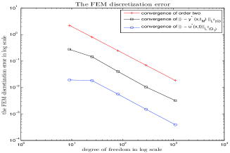
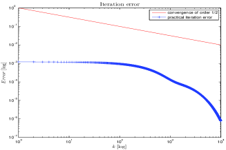
Figure 1: Example 5.1, $(\alpha,\beta)=(10^{-2},10)$. The left figure shows the FEM discretization errors with respect to d.o.f.. The right figure shows the iterative errors of correction full Jacobin decomposition method with respect to the $k$-iteration ($\|w^{k}-w^{*}\|_{H}$) in log-scale.

Further, in order to illustrate the parallel efficiency, we shall consider two cases for Example 5.1: (I) $h=1/32$ and $k=50,~{}100,~{}500,~{}1000,~{}5000,~{}10000$; (II) $k=10^{4}$ and $h=1/10,~{}1/20,~{}1/30,~{}1/40,~{}1/50,~{}1/60$. The time costs spent by using CPU-algorithm and GPU-algorithm, and the PSF are recorded in Table 1. For the sake of intuition, we also present the time costs of Table 1 in Figure 2. From the results in Table 1 and Figure 2, we can conclude that the growth rate of time cost of GPU-algorithm with the number of iterations is much smaller than that of CPU-algorithm in the case of $h=1/32$. For the fixed iteration number $k=10000$, the time cost of GPU-algorithm changes little with the change of mesh size, while the time cost of CPU-algorithm changes greatly. Specially, GPU-algorithm reduces the computation time sharply and PSF reaches $51.12$ when the mesh size $h=1/60$.

$h=1/32,k=$	50	100	500	1000	5000	10000
CPU(s)	3.60	9.95	108.04	223.92	1108.62	2192.23
GPU(s)	2.33	2.52	7.19	12.91	54.48	111.69
PSF	1.55	3.95	15.03	17.34	20.35	19.63
$k=10^{4},h=$	1/10	1/20	1/30	1/40	1/50	1/60
CPU(s)	7.74	35.41	1732.33	3867.60	5061.27	10525.36
GPU(s)	106.18	107.33	111.12	126.65	158.90	205.91
PSF	0.07	0.33	15.59	30.54	31.85	51.12

Table 1. Example 5.1, Comparison of CPU-algorithm and GPU-algorithm in computing time (s) and PSF.

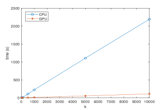
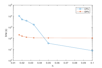
Figure 2: Example 5.1, $(\alpha,\beta)=(10^{-2},10)$. The time costs of CPU-algorithm and GPU-algorithm with respect to number of iterations with $h=1/32$ (left) and mesh size with $k=10^{4}$ (right).

For giving the interested readers a visual understanding, we present the numerical solutions $\mathbf{R_{x}}\{Y_{M}^{k}\}$ and $\mathbf{R_{x}}\{U_{M-\frac{1}{2}}^{k}\}$ with $h=1/32$ and $k=10^{4}$ in Figure 3. The results illustrate that the numerical solutions are coincided with the theoretical solutions $y^{*}$ and $u^{*}$, which verified the validity of the proposed method intuitively.

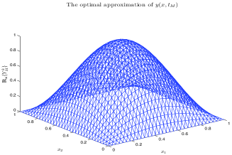
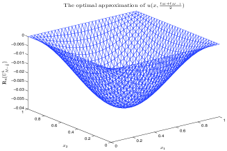
Figure 3: Example 5.1, $(\alpha,\beta)=(10^{-2},10)$. The numerical solutions $\mathbf{R_{x}}\{Y_{M}^{k}\}$ and $\mathbf{R_{x}}\{U_{M-\frac{1}{2}}^{k}\}$ with $h=1/32$ and $k=10^{4}$.

At the end of this example, we carry out the numerical experiment with the box constraint case $y\in[0,0.8]$. From the results exhibited in Figure  4, we can see that the numerical solution is reasonable.

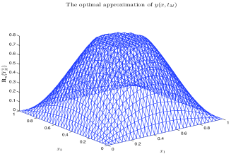
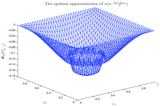
Figure 4: Example 5.1, $(\alpha,\beta)=(10^{-2},10)$. The numerical solutions $\mathbf{R_{x}}\{Y_{M}^{k}\}$ and $\mathbf{R_{x}}\{U_{M-\frac{1}{2}}^{k}\}$ with $h=1/32$ and $k=10^{4}$ under the box constraint case.

Example 5.2. (Neumann boundary condition) This example is taken from [1]. Assume $T=1$ in (1)-(2). Let the expected state function in the objective function be

$$y_{d}=c_{7}\omega_{a}(x,t)+c_{8}\omega_{b}(x,t)+c_{9}\omega_{a}(x,0)+c_{10}\omega_{b}(x,0)+c_{11}\omega_{a}(x,T)+c_{12}\omega_{b}(x,T)$$

with

$$\omega_{a}(x,t)=e^{\frac{1}{3}\pi^{2}t}\cos(\pi x_{1})\cos(\pi x_{2}),\quad\omega_{b}(x,t)=e^{-\frac{1}{3}\pi^{2}t}\cos(\pi x_{1})\cos(\pi x_{2}).$$

Set the source function $f=0$ and the homogeneous Neumann boundary condition as (3). It follows from the first order optimality condition (4) that the exact solution of (1)-(2) is

$$\begin{aligned} y^{*}=&~{}c_{1}\omega_{a}(x,t)+c_{2}\omega_{b}(x,t)+c_{3}\omega_{a}(x,0)+c_{4}\omega_{b}(x,0)+c_{5}\omega_{a}(x,T)+c_{6}\omega_{b}(x,T),\\ u^{*}=&~{}\frac{1}{3}\pi^{2}(c_{1}\omega_{a}(x,t)-c_{2}\omega_{b}(x,t))+y^{*}.\end{aligned}$$

Here the coefficients $\{c_{i}\}_{i=1}^{12}$ are specified in Table 2.

$c_{1}$	$c_{2}$	$c_{3}$	$c_{4}=c_{5}=c_{6}$
$\frac{-5\left(5e^{-\frac{1}{3}\pi^{2}}-6\right)}{-6+7e^{\frac{1}{3}\pi^{2}}}$	$5$	$\frac{7+141e^{\frac{1}{3}\pi^{2}}+7\left(e^{\frac{1}{3}\pi^{2}}\right)^{2}-6-106e^{-\frac{1}{3}\pi^{2}}}{4\left(6-7e^{\frac{1}{3}\pi^{2}}\right)}$	$\frac{1}{4}$
$c_{7}$	$c_{8}$	$c_{9}$	$c_{10}=c_{11}=c_{12}$
$\frac{5(9+35\alpha\pi^{4})\left(5e^{-\frac{1}{3}\pi^{2}}-6\right)}{9\left(6-7e^{\frac{1}{3}\pi^{2}}\right)}$	$5+\frac{175}{9}\alpha\pi^{4}$	$4\cdot c_{3}\cdot c_{10}$	$\frac{1}{4}+\alpha\pi^{4}$

Table 2. The coefficients $\{c_{i}\}_{i=1}^{12}$ of $y^{*}$, $u^{*}$, and $y_{d}$.

Now, we verify the convergence result in Theorem 5 by Example 5.2 with the parameters $(\alpha,\beta)=(10^{-3},10^{2})$. Figure 5(left) shows the convergence results of the FEM as functions of the mesh size $h$ when the iterative number $k=2\times 10^{4}$ is fixed. We can find that the convergence rates of the state variable $y$ at $t=T$ with norm $\|\cdot\|_{L^{2}(\Omega)}$ and the control variable $u$ with norm $\|\cdot\|_{L^{2}(Q_{T})}$ are both of order two, which are consistent with the theoretical results in Theorem 5. Next, we set the mesh size $h=1/64$ as the finest mesh. Figure 5(right) shows the errors of correction full Jacobin decomposition method ($\|w^{k}-w^{*}\|_{H}$) with respect to the $k$-iteration in log-scale. It is easy to see that the full Jacobin decomposition method with correction is faster than $O(\frac{1}{\sqrt{k}})$ as shown in Lemma 2.

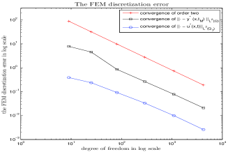
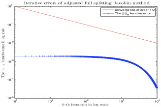
Figure 5: Example 5.2, $(\alpha,\beta)=(10^{-3},10^{2})$. The left figure shows the FEM discretization errors with respect to d.o.f.. The right figure shows the iterative errors of correction full Jacobin decomposition method with respect to the $k$-iteration ($\|w^{k}-w^{*}\|_{H}$) in log-scale.

Further, the computing times and PSF of Example 5.2 by using CPU-algorithm and GPU-algorithm are listed in Table 3 and Figure 6 with (I) $h=1/64$, $k=50,~{}100,~{}500,~{}1000,~{}5000,~{}10000$; (II) $k=10^{4}$ and $h=1/10,~{}1/20,~{}1/30,~{}1/40,~{}1/50,~{}1/60$. Compared with Example 5.1, the problem scale of Example 5.2 is larger, so the GPU-algorithm is more advantageous and the PSF could reach $76.17$.

$h=1/64,k=$	50	100	500	1000	5000	10000
CPU(s)	73.04	169.18	781.94	1625.20	8702.32	16380.33
GPU(s)	8.45	9.97	18.91	30.74	127.73	248.44
PSF	8.64	16.97	41.35	52.86	68.13	65.93
$k=10^{4},h=$	1/10	1/20	1/30	1/40	1/50	1/60
CPU(s)	13.13	50.71	3240.58	5087.63	10769.31	16001.93
GPU(s)	96.95	99.12	99.31	112.09	148.35	210.08
PSF	0.13	0.51	32.63	45.39	72.59	76.17

Table 3. Example 5.2, Comparsion of CPU-algorithm and GPU-algorithm in computing time (s) and PSF.

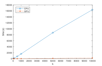
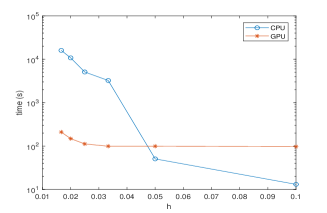
Figure 6: Example 5.2, $(\alpha,\beta)=(10^{-3},10^{2})$. The time costs of CPU-algorithm and GPU-algorithm with respect to number of iterations with $h=1/64$ (left) and mesh size with $k=10^{4}$ (right).

For giving the interested reader a visual understanding, we present the numerical solutions $\mathbf{R_{x}}\{Y_{M}^{k}\}$ and $\mathbf{R_{x}}\{U_{M-\frac{1}{2}}^{k}\}$ with $h=1/64$ and $k=2\times 10^{4}$ in Figure 7. The results could illustrate that the numerical solutions approximate the theoretical solutions $y^{*}$ and $u^{*}$ very well, which verified the validity of the proposed method intuitively.

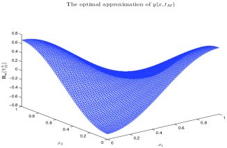
Figure 7: Example 5.2, $(\alpha,\beta)=(10^{-3},10^{2})$. The numerical solutions $\mathbf{R_{x}}\{Y_{M}^{k}\}$ and $\mathbf{R_{x}}\{U_{M-\frac{1}{2}}^{k}\}$ with $h=1/64$ and $k=2\times 10^{4}$.

Similar to Example 5.1, we present the numerical solutions of Example 5.2 with the box constraint case $y\in[-0.4,0.4]$ in Figure 8 at the end of this subsection.

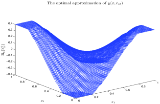
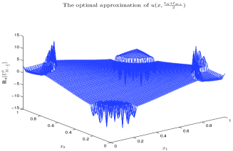
Figure 8: Example 5.2, $(\alpha,\beta)=(10^{-3},10^{2})$. The numerical solutions $\mathbf{R_{x}}\{Y_{M}^{k}\}$ and $\mathbf{R_{x}}\{U_{M-\frac{1}{2}}^{k}\}$ with $h=1/64$ and $k=2\times 10^{4}$ under the box constraint case.

6 Conclusions

In this paper, we propose an efficient parallel splitting method for the parabolic optimal control problems. The model problem is discretized by the Crank-Nicolson scheme and the numerical integration formula in temporal direction, and the linear finite element method in spatial direction. Based on the separable structure of the resulting large-scale optimization system, a full Jacobian decomposition method with correction is proposed, which improve the computational efficiency significantly. The global convergence estimation is established based on the FEM discretization error and the iteration error. Finally, numerical simulations are presented to verify the efficiency of the proposed algorithm.

References

- [1] T. Apel, T. G. Flaig. Crank-Nicolson schemes for optimal control problems with evolution equations. SIAM J. Numer. Anal., 50 (2012), 1484–1512.
- [2] D. Abbeloos, M. Diehl, M. Hinze, S. Vandewalle. Nested multigrid methods for time-periodic, parabolic optimal control problems. Comput. Vis. Sci., 14 (2011), 27–38.
- [3] A. Borz, G. von Winckel. Multigrid methods and sparse-grid collocation techniques for parabolic optimal control problems with random coefficients. SIAM J. Sci. Comput., 31 (2009), 2172–2192.
- [4] M. M. Butt and Y. Yuan. A full multigrid method for distributed control problems constrained by stokes equations. Numer. Math. Theor. Meth. Appl., 10 (2017), 639–655.
- [5] A. T. Barker, M. Stoll. Domain decomposition in time for PDE-constrained optimization. Comput. Phys. Commun., 197 (2015), 136–143.
- [6] E. Borgens, C. Kanzow. Regularized Jacobi-type ADMM-methods for a class of separable convex optimization problems in Hilbert spaces. Comput. Optim. Appl., 73 (2019), 755–790.
- [7] T. Carraro, M. Geiger, R. Rannacher. Indirect multiple shooting for nonlinear parabolic optimal control problems with control constraints. SIAM J. Sci. Comput., 36 (2014), A452–A481.
- [8] C. Chen, B. He, Y. Ye, X. Yuan. The direct extension of ADMM for multi-block convex minimization problems is not necessarily convergent. Math. Program., Ser. A, 155 (2016), 57–79.
- [9] Y. Chen, Y. Huang, N. Yi. A posteriori error estimates of spectral method for optimal control problems governed by parabolic equations. Sci. China Ser. A, 51 (2008), 1376–1390.
- [10] X. Du, M. Sarkis, C. Schaerer, D. Szyld. Inexact and truncated parareal-in-time Krylov subspace methods for parabolic optimal control problems. Electron. Trans. Numer. Anal., 40 (2013), 36–57.
- [11] H. Guan, D. Shi. A nonconforming finite element method for constrained optimal control problems governed by parabolic equations. Taiwanese J. Math., 21 (2017), 1193–1211.
- [12] W. Gong, N. Yan. Finite element approximations of parabolic optimal control problems with controls acting on a lower dimensional manifold. SIAM J. Numer. Anal., 54 (2016), 1229–1262.
- [13] M. Gunzburger. Perspectives in flow control and optimization. SIAM, 1987.
- [14] S. Gnther, N. R. Gauger, J. B. Schroder. A non-intrusive parallel-in-time approach for simultaneous optimization with unsteady PDEs. Optim. Methods Softw., 34 (2019), 1306–1321.
- [15] W. Gong, H. Xie, N. Yan. Adaptive multilevel correction method for finite element approximations of elliptic optimal control problems. J. Sci. Comput., 72 (2017), 820–841.
- [16] M. Hinze, R. Pinnau, M. Ulbrich, S. Ulbrich. Optimization with PDE Constraints. Mathematical Modelling: Theory and Applications. Springer, New York, 2009.
- [17] B. He, L. Hou, X. Yuan. On full Jacobian decomposition of the augmented Lagrangian method for separable convex programming. SIAM J. Optim., 25 (2015), 2274–2312.
- [18] T. Hou, Y. Chen, Y. Huang. A posteriori error estimates of mixed methods for quadratic optimal control problems governed by parabolic equations. Numer. Math. Theor. Meth. Appl., 4 (2011), 439–458.
- [19] F. Kwok. On the time-domain decomposition of parabolic optimal control problems. Domain decomposition methods in science and engineering XXIII, 55–67. Lect. Notes Comput. Sci. Eng., 116, Springer, Cham, 2017.
- [20] J. Liu, Z. Wang. Efficient time domain decomposition algorithms for parabolic PDE-constrained optimization problems. Comput. Math. Appl., 75 (2018), 2115–2133.
- [21] X. Luo, Y. Chen, Y. Huang, T. Hou. Some error estimates of finite volume element method for parabolic optimal control problems. Optimal Control Appl. Methods, 35 (2014), 145–165.
- [22] B. Li, J. Liu, M. Xiao. A new multigrid method for unconstrained parabolic optimal control problems. J. Comput. Appl. Math., 326 (2017), 358–373.
- [23] W. Liu, H. Ma, T. Tang, N. Yan. A posteriori error estimates for discontinuous Galerkin time-stepping method for optimal control problems governed by parabolic equations. SIAM J. Numer. Anal., 42 (2004), 1032–1061.
- [24] D. Meidner, B. Vexler. A priori error estimates for space-time finite element discretization of parabolic optimal control problems. I. Problems without control constraints. SIAM J. Control Optim., 47 (2008), 1150–1177.
- [25] D. Meidner, B. Vexler. A priori error estimates for space-time finite element discretization of parabolic optimal control problems. II. Problems with control constraints. SIAM J. Control Optim., 47 (2008), 1301–1329.
- [26] J. W. Pearson, A. J. Wathen. A new approximation of the Schur complement in preconditioners for PDE-constrained optimization. Numer. Linear Algebra Appl., 19 (2012), 816–829.
- [27] J. W. Pearson, M. Stoll, A. J. Wathen. Regularization-robust preconditioners for time-dependent PDE-constrained optimization problems. SIAM J. Matrix Anal. Appl., 33 (2012), 1126–1152.
- [28] M. K. Riahi. A new approach to improve ill-conditioned parabolic optimal control problem via time domain decomposition. Numer. Algorithms, 72 (2016), 635–666.
- [29] Anton. Schiela, S. Ulbrich. Operator preconditioning for a class of inequality constrained optimal control problems. SIAM J. Optim., 24 (2014), 435–466.
- [30] M. Stoll, T. Breiten. A low-rank in time approach to PDE-constrained optimization. SIAM J. Sci. Comput., 37 (2015), B1–B29.
- [31] F. Trltzsch. Optimal control of partial differential equations. AMS, Providence, RI, 2010.
- [32] M. Wu, W. Ai, J. Yuan, H. Tian. A symmetric inertial alternating direction method of multipliers for elliptic equation constrained optimization problem, Adv. Appl. Math. Mech., (2021), doi:10.4208/aamm.OA-2020-0400.
- [33] H. Yang, F. Hwang, X. Cai. Nonlinear preconditioning techniques for full-space Lagrange-Newton solution of PDE-constrained optimization problems. SIAM J. Sci. Comput., 38 (2016), A2756–A2778.
- [34] C. Yang, T. Wang, X. Xie, An interface-unfitted finite element method for elliptic interface optimal control problems. Numer. Math. Theor. Meth. Appl., 12 (2019), 727–749.