Low-Complexity Pareto-Optimal 3D Beamforming for the Full-Dimensional Multi-User Massive MIMO Downlink

Abstract

Full-dimensional (FD) multi-user massive multiple-input multiple output (m-MIMO) systems employ large two-dimensional (2D) rectangular antenna arrays to control both the azimuth and elevation angles of signal transmission. We introduce the sum of two outer products of the azimuth and elevation beamforming vectors having moderate dimensions as a new class of FD beamforming. We show that this low-complexity class is capable of outperforming 2D beamforming relying on the single outer product of the azimuth and elevation beamforming vectors. It is also capable of performing close to its FD counterpart of massive dimensions in terms of either the users’ minimum rate or their geometric mean rate (GM-rate), or sum rate (SR). Furthermore, we also show that even FD beamforming may be outperformed by our outer product-based improper Gaussian signaling solution. Explicitly, our design is based on low-complexity algorithms relying on convex problems of moderate dimensions for max-min rate optimization or on closed-form expressions for GM-rate and SR maximization.

I Introduction

Full-dimensional (FD) massive multi-input multi-output (m-MIMO) schemes [1, 2, 3, 4] relying on a large two-dimensional (2D) uniformly spaced rectangular antenna array (URA) have emerged as a practical m-MIMO implementation. The design of FD m-MIMO systems in terms of antenna tilts has been considered e.g. in [5, 6, 7, 8, 9] and in the references therein.

As the degree of freedom in FD m-MIMO systems is reduced by the channels’ spatial correlations, it is more practical to serve a large number of single-antenna users than a small number of multiple-antenna users. The beamforming design of optimizing the users’ rate in m-MIMO systems is computationally complex even for the popular zero-forcing (ZF) or regularized zero-forcing (RZF) or conjugate beamforming (CB) scenarios, since it must rely on iteratively solving convex problems of high dimensions [10, 11, 12]. For FD systems, the most popular 2D beamformer relies on beamforming matrices (BMs) represented by the single outer product of the azimuth beamformer (AB) and elevation beamformer [13, 14, 15, 16, 17]. These ABs and EBs have been separately designed in [13] for the specific scenario of a single user, and in [17] for multiple users. Their joint design has been considered in [15] with the objective of maximizing the sum rate using semi-definite relaxation, which imposed an extremely high computational complexity. All these contributions considered FD of moderate dimensions, rather than of massive dimensions, as in m-MIMO schemes. Hence it is of substantial interest in practice to investigate particular classes of FD beamforming capable of mitigating the design complexity of FD m-MIMO systems.

Subject to the sum transmit power constraint, the beamforming design aims for maximizing either the sum rate (SR) or the users’ minimum rate (MR). The SR problem has been widely studied thanks to its tractable formulation, which is based on iterating upon evaluating low-complexity closed-form expressions. However, it leads to assigning a large fraction of the total SR to a few privileged users having the best channel conditions, leaving only low rates for all other users and thus having a potentially zero MR. Maximizing the MR may only be achieved at the cost of degrading the total SR, and it is also computationally challenging, since its computation must be based on iterating by evaluating large-scale convex problems [18, 19, 20] to handle the non-differentiable objective function and thus it is not practical for m-MIMO systems. One can potentially balance the SR and MR by maximizing the SR subject to a constraint on MR, but this is computationally challenging. Our previous papers [21, 22, 23, 24] have shown that the geometric mean of the users’ rates (GM-rate) is a beneficial objective function, since its maximization leads to a similar rate for all users without having to impose MR constraints, while still maintaining a good SR. Hence the solution becomes reminiscent of a Pareto optimal solution constructed for optimizing the twice-objective SR and MR problem. As strong duality holds under very mild conditions for single-constrained optimization [25], [26, Chaper 10.2], the GM-rate problem considered leads itself to convenient tractable computation, despite the fact that the GM-rate objective function is nonconcave (but differentiable).

Recent studies such as [27, 28, 29, 30, 31, 20, 21] and the references therein have shown that improper Gaussian signaling (IGS) – which transmits improper Gaussian signals instead of the conventional proper Gaussian signals – is capable of increasing the users’ rate. However, the beamforming design problem of IGS is much more complex than that under conventional proper Guassian signaling, because each information source intended for each user is beamformed by relying on a pair of vectors – rather than on a single one – for which the user rate is defined by a log-determinant function.

Against the above background, this paper is the first one to consider the multi-user beamforming design of FD m-MIMO systems. The contributions of this paper are three-fold:

• We define the sum of a few outer products of the ABs and EBs having moderate dimensions as a new FD beamforming structure, which includes both the 2D and FD beamforming classes as a particular case. More importantly, it is shown that the sum of two outer products is capable of outperforming 2D beamforming. It also performs similarly to the FD class in terms of the users’ MR, or GM-rate, or SR, despite its lower design complexity. Therefore, the sum-of-two-outer-product may be deemed to be the optimal structure of FD beamforming;

• We develop a new class of improper Gaussian signaling, which is based on sum-pairs of the outer products, which is shown to outperform the FD class;

• We develop low-complexity algorithms for designing all the beamformers, which are based on convex problems of moderate dimension for iteratively improving the MR in MR maximization. However, MR maximization results in low SR.

• Furthermore, we develop closed-form expressions for iteratively improving the GM-rate and SR. However, SR maximization results in zero rates for the users having low channel quality and thus it is not suitable for providing a fair service for all users. Our simulations reveal that GM-rate maximization is computationally attractive and it strikes a compelling trade-off between conflicted MR and SR for Pareto optimization.

The contributions of this work are boldly and explicitly contrasted to the literature in Table I.

TABLE I: Boldly contrasting our novel contributions to the related literature.

	This work	[5, 9]	[7, 8]	[15]	[16]	[6, 17]
FD m-MIMO	$\surd$				$\surd$
FD beamforming	$\surd$	$\surd$
2D beamforming	$\surd$		$\surd$	$\surd$	$\surd$	$\surd$
New low-complex beamforming	$\surd$
Heuristic methods		$\surd$	$\surd$	$\surd$	$\surd$	$\surd$
Low computational complexity	$\surd$	$\surd$				$\surd$
High computational complexity			$\surd$	$\surd$	$\surd$
Pareto optimization	$\surd$

The paper is organized as follows. Section II proposes a new class of FD beamforming, whose computational solution is developed in Section III. Section IV introduces a new class of improper Gaussian signaling, which uses pairs of the sums of outer products, together with a supporting computational solution. Our numerical examples are given in Section V, while Section VI concludes the paper.

Notation. Only the vector/matrix variables are printed in boldface; $I_{N}$ is the identity matrix of size $N\times N$. $[X]^{2}$ is $XX^{H}$, $\langle X,Y\rangle=\mbox{trace}(X^{H}Y)$, which is the dot product of the matrices $X$ and $Y$. We also write $\langle X\rangle=\mbox{trace}(X)$ for notational simplicity. Accordingly, the Frobenius norm of $X$ is defined by $||X||=\sqrt{\langle[X]^{2}\rangle}$. Furthermore, $X\succeq 0$ means that the matrix $X$ is positive semi-definite. ${\sf vect}(.)$ arranges the matrix into a vector by stacking its columns, while ${\sf Col}(x_{k})_{k\in{\cal K}}$ arranges the columns $x_{k}$, $k\in{\cal K}\triangleq\{1,\dots,K\}$ in the single column $\begin{bmatrix}x_{1}^{T}&\dots&x_{K}^{T}\end{bmatrix}^{T}$, and ${\sf Row}(x_{k})_{k\in{\cal K}}$ arranges the rows $x_{k}$, $k\in{\cal K}$, in the single row $\begin{bmatrix}x_{1}&\dots&x_{K}\end{bmatrix}^{T}$. Lastly, let us denote the set of circular Gaussian random variables having zero means and variance $a$ by ${\cal C}(0,a)$.

The following inequalities, which were derived in [18], are frequently used in our theoretical development:

$$\ln\left(1+\frac{|v|^{2}}{y+\sigma}\right)\geq\alpha(\bar{v},\bar{y})+2\frac{\Re\{\bar{v}^{*}v\}}{\bar{y}+\sigma}-\psi(\bar{v},\bar{y})(|v|^{2}+y),$$ (1)

with

$$\begin{array}[]{c}\alpha(\bar{v},\bar{y})\triangleq\ln\left(1+\frac{|\bar{v}|^{2}}{\bar{y}}\right)-\frac{|\bar{v}|^{2}}{\bar{y}}-\sigma\psi(\bar{v},\bar{y}),\\ 0<\psi(\bar{v},\bar{y})\triangleq\frac{|\bar{v}|^{2}}{(\bar{y}+\sigma)(|\bar{v}|^{2}+\bar{y}+\sigma)}\end{array}$$ (2)

for all $v\in\mathbb{C}$, $y\geq 0$, $\sigma>0$, and $\bar{v}\in\mathbb{C}$, $\bar{y}\geq 0$, and

$$\ln\left|I_{2}+[V]^{2}(Y+\sigma I_{2})^{-1}\right|\geq\alpha(\bar{V},\bar{Y})$$

$$+2\Re\{\langle(\bar{Y}+\sigma I_{2})^{-1}\bar{V},V\rangle\}-\langle\Psi(\bar{V},\bar{Y}),[V]^{2}+Y\rangle,$$ (3)

with

$$\begin{array}[]{c}\alpha(\bar{V},\bar{Y})\triangleq\ln\left|I_{2}+[\bar{V}]^{2}(\bar{Y}+\sigma I_{2})^{-1}\right|\\ -\langle(\bar{Y}+\sigma I_{2})^{-1},[\bar{V}]^{2}\rangle-\sigma\langle\Psi(\bar{V},\bar{Y})\rangle,\\ 0\preceq\Psi(\bar{V},\bar{Y})\triangleq(\bar{Y}+\sigma I_{2})^{-1}-([\bar{V}]^{2}+\bar{Y}+\sigma I_{2})^{-1}\end{array}$$ (4)

for all matrices $V$, $Y\succ 0$, $\bar{V}$, and $\bar{Y}\succ 0$ of size $2\times 2$, and $\sigma>0$. Considering both sides of (1) and (I) as functions of $(v,y)$ and $(V,Y)$, which match each other at $(\bar{v},\bar{y})$ and $(\bar{V},\bar{Y})$, the functions in the right hand side (RHS) provide tight minorants of their counterparts in the left hand side (LHS) [26].

II Low-complexity structured beamforming

We consider a network of a base station (BS) equipped with a $M\times M$-URA to serve $K$ single-antenna downlink users (UEs), which are indexed by $k\in{\cal K}\triangleq\{1,\dots,K\}$. Let $H_{k}\in\mathbb{C}^{M\times M}$ represent the channel matrix spanning from the BS’ URA to UE $k$, i.e. each of its entry $H_{k}(m,n)$ characterizes the link spanning from the $(m,n)$-th antenna to UE $k$.

Let $s_{k}\in{\cal C}(0,1)$ be the information symbol intended for UE $k\in{\cal K}$, which is beamformed by the matrix $\mathbf{W}_{k}\in\mathbb{C}^{M\times M}$ for the BS’s downlink (DL) transmission, i.e. the $(m,n)$-th antenna transmits the signal $\sum_{k=1}^{K}\mathbf{W}_{k}(m,n)s_{k}$. The DL signal received at UE $k$ is given by

$$y_{k} = \sum_{k^{\prime}=1}^{K}\langle H_{k}^{T}\mathbf{W}_{k^{\prime}}\rangle s_{k^{\prime}}+n_{k},$$ (5)

where $n_{k}\in{\cal C}(0,\sigma)$ is the noise, which incorporates both the background noise and other uncertainties, such as the channel estimation error [32]. The robust design relying on imperfect channel state information, which explicitly incorporates the channel estimation error into the optimization formulation is beyond the scope of this paper. Based on the following simplified rank-one model of $H_{k}$:

$$H_{k}=h_{k}^{e}(h_{k}^{a})^{T},$$ (6)

with $h_{k}^{a}\in\mathbb{C}^{M}$ representing azimuth span while $h_{k}^{e}\in\mathbb{C}^{M}$ representing the elevation span, the following $2$D beamformer of rank one has been proposed in [13, 14, 15, 16, 17]:

$$\mathbf{W}_{k}=\mathbf{w}^{e}_{1,k}(\mathbf{w}^{a}_{1,k})^{T},$$ (7)

where $\mathbf{w}^{a}_{1,k}\in\mathbb{C}^{M}$ and $\mathbf{w}^{e}_{1,k}\in\mathbb{C}^{M}$ are termed as the AB and EB, respectively. In this paper, we propose the following new structure of $\mathbf{W}_{k}\in\mathbb{C}^{M\times M}$ of rank $Q$

$$\mathbf{W}_{k}=\sum_{q=1}^{Q}\mathbf{w}^{e}_{q,k}(\mathbf{w}^{a}_{q,k})^{T},$$ (8)

with

$$\mathbf{w}^{\chi}_{q,k}\in\mathbb{C}^{M},\chi\in\{a,e\},q\in\mathcal{Q}\triangleq\{1,\dots,Q\}.$$ (9)

In other words, each beamforming matrix (BM) $\mathbf{W}_{k}\in\mathbb{C}^{M\times M}$ is a sum of $Q$ outer products $\mathbf{w}^{e}_{q,k}(\mathbf{w}^{a}_{q,k})^{T}$, $q\in\mathcal{Q}$, each of which is termed as a 2D BM. As expected, the $2D$ beamformer (7) is a particular case of (8) for $Q=1$, while the unstructured FD $\mathbf{W}_{k}\in\mathbb{C}^{M\times M}$ is also a particular case of (8) for $Q=M$. Note that each BM $\mathbf{W}_{k}$ in (8) is characterized by $2QM$ decision variables, while each $2D$ BM in (7) is characterized by $2M$ decision variables. Looking ahead, in the simulations we will show that the BM $\mathbf{W}_{k}$ defined by (8) for $Q=2$ already performs similarly well to the FD ones, even though the latter are characterized by $M^{2}$ decision variables.

With $\mathbf{W}_{k}$ defined by (8), equation (5) of the DL signal received at UE $k$ becomes

$$y_{k}=\sum_{k^{\prime}=1}^{K}\left(\sum_{q=1}^{Q}(\mathbf{w}^{e}_{q,k^{\prime}})^{T}H_{k}\mathbf{w}^{a}_{q,k^{\prime}}\right)s_{k^{\prime}}+n_{k}.$$ (10)

In what follows, we will use the notations

$$\mathbf{w}^{\chi}_{k}\triangleq{\sf Col}(\mathbf{w}^{\chi}_{q,k})_{q\in\mathcal{Q}}\in\mathbb{C}^{QM},\chi\in\{a,e\},$$ (11)

and then $\mathbf{w}^{a}\triangleq\{\mathbf{w}^{a}_{k},k\in{\cal K}\}$, and $\mathbf{w}^{e}\triangleq\{\mathbf{w}^{e}_{k},k\in{\cal K}\}$, and $\mathbf{w}\triangleq\{\mathbf{w}^{a},\mathbf{w}^{e}\}$. The rate at UE $k$ is

$$r_{k}(\mathbf{w}^{a},\mathbf{w}^{e})\triangleq\ln\left[1+g_{k}(\mathbf{w}^{a},\mathbf{w}^{e})\right],$$ (12)

where we have

$$g_{k}(\mathbf{w}^{a},\mathbf{w}^{e})\triangleq\frac{|\sum_{q=1}^{Q}(\mathbf{w}_{q,k}^{e})^{T}H_{k}\mathbf{w}^{a}_{q,k}|^{2}}{\sum_{k^{\prime}\in{\cal K}\setminus\{k\}}|\sum_{q=1}^{Q}(\mathbf{w}_{q,k^{\prime}}^{e})^{T}H_{k}\mathbf{w}^{a}_{q,k^{\prime}}|^{2}+\sigma}.$$ (13)

Given the power budget $P$, we are interested in the following three problems of sum-power constrained Pareto beamforming optimization:

$$\max_{\mathbf{w}=(\mathbf{w}^{a},\mathbf{w}^{e})}\ \varphi_{SR}(\mathbf{w}^{a},\mathbf{w}^{e})\triangleq\sum_{k=1}^{K}r_{k}(\mathbf{w}^{a},\mathbf{w}^{e})$$ (14a)

$$\mbox{s.t.}\quad\sum_{k=1}^{K}||\sum_{q=1}^{Q}\mathbf{w}^{a}_{q,k}(\mathbf{w}^{e}_{q,k})^{T}||^{2}\leq P,$$ (14b)

for maximizing the SR as well as

$$\max_{\mathbf{w}=(\mathbf{w}^{a},\mathbf{w}^{e})}\ \varphi_{MR}(\mathbf{w}^{a},\mathbf{w}^{e})\triangleq\min_{k=1,\dots,K}r_{k}(\mathbf{w}^{a},\mathbf{w}^{e})$$

$$\mbox{s.t.}\quad(\ref{tra4b}),$$ (15)

for maximizing the MR, and

$$\max_{\mathbf{w}=(\mathbf{w}^{a},\mathbf{w}^{e})}\ \varphi_{GM}(\mathbf{w}^{a},\mathbf{w}^{e})\triangleq\left(\prod_{k=1}^{K}r_{k}(\mathbf{w}^{a},\mathbf{w}^{e})\right)^{1/K}$$

$$\mbox{s.t.}\quad(\ref{tra4b}),$$ (16)

for maximizing the GM-rate. We will compare the SR, MR, and GM-rate performances attained by the beamforming class (8) to that by their FD counterparts $\mathbf{W}\triangleq\{\mathbf{W}_{k}\in\mathbb{C}^{M\times M},k\in{\cal K}\}$:

$$\max_{\mathbf{W}}\ f_{SR}(\mathbf{W})\triangleq\sum_{k=1}^{K}r_{k}(\mathbf{W})$$ (17a)

$$\mbox{s.t.}\quad\sum_{k=1}^{K}||\mathbf{W}_{k}||^{2}\leq P,$$ (17b)

and

$$\max_{\mathbf{W}}\ f_{MR}(\mathbf{W})\triangleq\min_{k=1,\dots,K}r_{k}(\mathbf{W})\quad\mbox{s.t.}\quad(\ref{sfdb3b}),$$ (18)

and

$$\max_{\mathbf{W}}\ f_{GM}(\mathbf{W})\triangleq\left(\prod_{k=1}^{K}r_{k}(\mathbf{W})\right)^{1/K}\quad\mbox{s.t.}\quad(\ref{sfdb3b}),$$ (19)

where

$$r_{k}(\mathbf{W})=\ln\left(1+\frac{|\langle H_{k},\mathbf{W}_{k}\rangle|^{2}}{\sum_{k^{\prime}\in{\cal K}\setminus\{k\}}|\langle H_{k},\mathbf{W}_{k^{\prime}}\rangle|^{2}+\sigma}\right).$$ (20)

As aforementioned, the SR problem (17) is computationally tractable but it leads to very low rates for users having less favorable channel conditions and thus zero MR. The MR problem (18) is computationally difficult, since its computation must be based on iterating large-scale convex problems having the computational complexity order of ${\cal O}(K^{3}M^{6})$ [18, 19, 20] and thus it is not practical for FD m-MIMO systems. One can overcome the zero-rate issue of the SR problem (17) by enforcing the additional MR constraint $f_{MR}(\mathbf{W})\geq r_{\min}$ for a given $r_{\min}$ to solve the problem

$$\max_{\mathbf{W}}f_{SR}(\mathbf{W})\quad\mbox{s.t.}\quad(\ref{sfdb3b}),f_{MR}(\mathbf{W})\geq r_{\min},$$ (21)

which is however even more computationally intractable than the MR problem (18). This is because the MR constraint in the former is nonconvex and thus computationally intractable, while the single sum-power constraint in the latter is convex and thus it is computationally tractable. It has been shown in our previous papers [21, 22, 23, 24] that maximizing the GM-rate objective function $f_{GM}(\mathbf{W})$ leads to similar rates for all users without enforcing the MR constraint $f_{MR}(\mathbf{W})\geq r_{\min}$, while still maintaining a good SR. Hence again, the resultant solution is reminiscent of a Pareto optimal solution constructed for optimizing the twice-objective SR and MR problem. Importantly, we will show that the computational complexity of maximizing the GM-rate objective function is appealingly low, because it is based on iterating by evaluating closed-form expressions. Another distinct hallmark of maximizing the GM-rate objective in (19) that will be highlighted by simulations is the resultant similar transmit powers at the antennas. This allows us to circumvent the per-antenna transmit power constraints that were deemed important in the m-MIMO implementation of [33]. In other words, problem (II) of maximizing the GM-rate subject to a single sum-power constraint (14b) provides a refreshingly new approach to m-MIMO designs capable of maintaining similar user rates, despite using similar DL transmit powers at each antenna.

The next section is devoted to the computational solution of the problems (14)-(II) and their FD counterparts (17)-(19).

III Optimization algorithms

The first two subsections propose algorithms for computing (14)-(II), while the last subsection proposes algorithms for computing (17)-(19).

In what follows, we use a feasible initialization of $(w^{a,(0)},w^{e,(0)})$ for (14b) and then $w^{(\kappa)}\triangleq(w^{a,(\kappa)},w^{e,(\kappa)})$ denotes a feasible point of (14b) that is found from the $(\kappa-1)$-st iteration for $\kappa=1,2,\dots$. The $\kappa$-th iteration is used for generating $w^{(\kappa+1)}=(w^{a,(\kappa+1)},w^{e,(\kappa+1)})$ as follows.

III-A MR optimization algorithm

III-A1 AB alternating optimization

With $\mathbf{w}^{e}$ held fixed at $w^{e,(\kappa)}$, the constraint (14b) becomes

$$\sum_{k=1}^{K}\langle\mathcal{Q}^{e,(\kappa)}_{k},[\mathbf{w}^{a}_{k}]^{2}\rangle\leq P,$$ (22)

where

$$0\!\preceq\!\mathcal{Q}^{e,(\kappa)}_{k}\!\triangleq\!\begin{bmatrix}\langle w^{e,(\kappa)}_{q,k},w^{e,(\kappa)}_{q^{\prime},k}\rangle I_{M}\end{bmatrix}_{(q,q^{\prime})\in\mathcal{Q}\times\mathcal{Q}}\in\mathbb{C}^{(QM)\times(QM)}.$$ (23)

For $(k^{\prime},k)\in{\cal K}\times{\cal K}$, we define

$$h^{e,(\kappa)}_{k^{\prime},k}\triangleq{\sf Row}((w^{e,(\kappa)}_{q,k^{\prime}})^{T}H_{k})_{q\in\mathcal{Q}}\in\mathbb{C}^{1\times(QM)},$$ (24)

to write

$$r_{k}(\mathbf{w}^{a},w^{e,(\kappa)}) =r^{a}_{k}(\mathbf{w}^{a})$$

$$\triangleq\ln\left(1+\frac{|h^{e,(\kappa)}_{k,k}\mathbf{w}^{a}_{k}|^{2}}{\sum_{k^{\prime}\in{\cal K}\setminus\{k\}}|h^{e,(\kappa)}_{k^{\prime},k}\mathbf{w}^{a}_{k^{\prime}}|^{2}+\sigma}\right).$$ (25)

To seek an AB $w^{a,(\kappa+1)}$ so that

$$\varphi_{MR}(w^{a,(\kappa)},w^{e,(\kappa)})<\varphi_{MR}(w^{a,(\kappa+1)},w^{e,(\kappa)}),$$ (26)

we consider the following problem:

$$\max_{\mathbf{w}^{a}}\min_{k=1,\dots,K}r^{a}_{k}(\mathbf{w}^{a})\quad\mbox{s.t.}\quad(\ref{taa5b}).$$ (27)

For $(\bar{v}_{k},\bar{y}_{k})\triangleq(h^{e,(\kappa)}_{k,k}w^{a,(\kappa)}_{k},\sum_{k^{\prime}\in{\cal K}\setminus\{k\}}|h^{e,(\kappa)}_{k^{\prime},k}w^{a,(\kappa)}_{k^{\prime}}|^{2})$, and accordingly $\alpha(\bar{v}_{k},\bar{y}_{k})$ and $\psi(\bar{v}_{k},\bar{y}_{k})$ defined by (2), applying the inequality (1) yields the following tight minorant of $r^{a}_{k}(\mathbf{w}^{a})$ at $w^{a,(\kappa)}$:

$$r^{a,(\kappa)}_{k}(\mathbf{w}^{a})\triangleq a^{a,(\kappa)}_{k}+2\Re\{b^{a,(\kappa)}_{k}\mathbf{w}^{a}_{k}\}-c^{a,(\kappa)}_{k}\sum_{k^{\prime}=1}^{K}|h^{e,(\kappa)}_{k^{\prime},k}\mathbf{w}^{a}_{k^{\prime}}|^{2},$$ (28)

for

$$a^{a,(\kappa)}_{k}\triangleq\alpha(\bar{v}_{k},\bar{y}_{k}),b^{a,(\kappa)}_{k}\triangleq\frac{\bar{v}^{*}_{k}}{\bar{y}_{k}+\sigma}h^{e,(\kappa)}_{k,k},c^{a,(\kappa)}_{k}\triangleq\psi(\bar{v}_{k},\bar{y}_{k}).$$ (29)

Thus, we generate $w^{a,(\kappa+1)}$ as the optimal solution of the following convex quadratic problem of tight minorant maximization:

$$\max_{\mathbf{w}^{a}}\min_{k=1,\dots,K}r^{a,(\kappa)}_{k}(\mathbf{w}^{a})\quad\mbox{s.t.}\quad(\ref{taa5b}).$$ (30)

As $w^{a,(\kappa)}$ and $w^{a,(\kappa+1)}$ constitute a feasible point and the optimal solution of (30), we have (26) as long as $\varphi_{MR}(w^{a,(\kappa+1)},w^{e,(\kappa)})\neq\varphi_{MR}(w^{a,(\kappa)},w^{e,(\kappa)})$.

III-A2 EB alternating optimization

With $\mathbf{w}^{a}$ held fixed at $w^{a,(\kappa+1)}$, the constraint (14b) becomes

$$\sum_{k=1}^{K}\langle\mathcal{Q}^{a,(\kappa)}_{k},[\mathbf{w}^{e}_{k}]^{2}\rangle\leq P,$$ (31)

with

$$0\preceq\mathcal{Q}^{a,(\kappa)}_{k}\triangleq\begin{bmatrix}\langle w^{a,(\kappa+1)}_{q,k},w^{a,(\kappa+1)}_{q^{\prime},k}\rangle I_{M}\end{bmatrix}_{(q,q^{\prime})\in\mathcal{Q}\times\mathcal{Q}}$$

$$\in\mathbb{C}^{(QM)\times(QM)}.$$ (32)

Upon defining

$$h^{a,(\kappa)}_{k^{\prime},k}\triangleq{\sf Row}((w^{a,(\kappa+1)}_{q,k^{\prime}})^{T}H_{k}^{T})_{q\in\mathcal{Q}}\in\mathbb{C}^{1\times(QM)},$$ (33)

we may write

$$r_{k}(w^{a,(\kappa+1)},\mathbf{w}^{e}) =r^{e}_{k}(\mathbf{w}^{a})$$

$$\triangleq\ln\left(1+\frac{|h^{a,(\kappa)}_{k,k}\mathbf{w}^{e}_{k}|^{2}}{\sum_{k^{\prime}\in{\cal K}\setminus\{k\}}|h^{a,(\kappa)}_{k^{\prime},k}\mathbf{w}^{e}_{k^{\prime}}|^{2}+\sigma}\right).$$ (34)

Thus, to seek an EB $w^{e,(\kappa+1)}$ so that

$$\varphi_{MR}(w^{a,(\kappa+1)},w^{e,(\kappa)})<\varphi_{MR}(w^{a,(\kappa+1)},w^{e,(\kappa+1)}),$$ (35)

we consider the following problem:

$$\max_{\mathbf{w}^{e}}\min_{k=1,\dots,K}r^{e}_{k}(\mathbf{w}^{e})\quad\mbox{s.t.}\quad(\ref{tea5b}).$$ (36)

For $(\bar{v}_{k},\bar{y}_{k})\triangleq(h^{a,(\kappa)}_{k,k}w^{e,(\kappa)}_{k},\sum_{k^{\prime}\in{\cal K}\setminus\{k\}}|h^{a,(\kappa)}_{k^{\prime},k}w^{e,(\kappa)}_{k^{\prime}}|^{2})$ and according to $\alpha(\bar{v}_{k},\bar{y}_{k})$ and $\psi(\bar{v}_{k},\bar{y}_{k})$ defined by (2), applying the inequality (1) yields the following tight concave quadratic minorant of the function $r^{e}_{k}(\mathbf{w}^{e})$ at $w^{e,(\kappa)}$:

$$r^{e,(\kappa)}_{k}(\mathbf{w}^{e})\triangleq a^{e,(\kappa)}_{k}+2\Re\{b^{e,(\kappa)}_{k}\mathbf{w}^{e}_{k}\}-c^{e,(\kappa)}_{k}\sum_{k^{\prime}=1}^{K}|h^{a,(\kappa)}_{k^{\prime},k}\mathbf{w}^{e}_{k^{\prime}}|^{2},$$ (37)

for

$$a^{e,(\kappa)}_{k}\triangleq\alpha(\bar{v}_{k},\bar{y}_{k}),b^{e,(\kappa)}_{k}\triangleq\displaystyle\frac{\bar{v}^{*}_{k}}{\bar{y}_{k}+\sigma}h^{a,(\kappa)}_{k,k},c^{e,(\kappa)}_{k}\triangleq\psi(\bar{v}_{k},\bar{y}_{k}).$$ (38)

Thus, we generate $w^{e,(\kappa+1)}$ as the optimal solution of the following convex quadratic problem of tight minorant maximization of (36):

$$\max_{\mathbf{w}^{e}}\min_{k=1,\dots,K}r^{e,(\kappa)}_{k}(\mathbf{w}^{e})\quad\mbox{s.t.}\quad(\ref{tea5b}).$$ (39)

Similar to (26), we have (35) as far as $\varphi_{MR}(w^{a,(\kappa+1)},w^{e,(\kappa+1)})\neq\varphi_{MR}(w^{a,(\kappa+1)},w^{e,(\kappa)})$.

III-A3 The algorithm and its computational complexity

Algorithm 1 provides the pseudo-code for the proposed computational procedure. The sequence $\{(w^{a,(\kappa)},w^{e,(\kappa)})\}$ is composed of improved feasible points of problem (II) and thus it converges to a point $(\bar{w}^{a},\bar{w}^{e})$ according to Cauchy’s theorem, which satisfies the first-order optimality condition with $\mathbf{w}^{e}$ ($\mathbf{w}^{a}$, resp.) held fixed at $\bar{w}^{e}$ ($\bar{w}^{a}$, resp.). The computational complexity of each of its iteration is on the order of

$$\mathcal{O}(K^{3}Q^{3}M^{3}),$$ (40)

which is the computational complexity of (30) and (39) [34]. Clearly, this involves $KQM$ decision variables.

III-B SR and GM-rate maximization algorithms

With the concave functions $r^{a,(\kappa)}_{k}$ and $r^{e,(\kappa)}_{k}$ defined from (28) and (37), their GMs $(\prod_{k=1}^{K}r^{a,(\kappa)}_{k})^{1/K}$ and $(\prod_{k=1}^{K}r^{e,(\kappa)}_{k})^{1/K}$ are still concave functions [26, Prop. 2.7]. Therefore, like Algorithm 1, the following Algorithm 2 generates a sequence of $\{(w^{a,(\kappa)},w^{e,(\kappa)})\}$ such that

$$\varphi_{GM}(w^{a,(\kappa)},w^{e,(\kappa)}) <\varphi_{GM}(w^{a,(\kappa+1)},w^{e,(\kappa)})$$

$$<\varphi_{GM}(w^{a,(\kappa+1)},w^{e,(\kappa+1)}),$$ (41)

which converges to a point $(\bar{w}^{a},\bar{w}^{e})$ that satisfies the first-order optimality condition with $\mathbf{w}^{e}$ ($\mathbf{w}^{a}$, resp.) held fixed at $\bar{w}^{e}$ ($\bar{w}^{a}$, resp.). However, the computational complexity of each of its iteration is given by (40).

Now, following [21, 22, 23, 24] we develop another algorithm for computing (II), which is based on iterating by evaluating closed-form expressions and thus it is much more computationally efficient than Algorithm 2. More importantly, our simulations will show that both Algorithms 2 and 3 below perform similarly, so the advantage of the latter is plausible.

Upon defining $\varphi_{GM}(\mathbf{w}^{a},\mathbf{w}^{e})=\Phi_{GM}[r_{1}(\mathbf{w}^{a},\mathbf{w}^{e}),\dots,r_{K}(\mathbf{w}^{a},\mathbf{w}^{e})]$ in conjunction with

$$\Phi_{GM}(r_{1},\dots,r_{K})\triangleq\left(\prod_{k=1}^{K}r_{k}(\mathbf{w}^{a},\mathbf{w}^{e})\right)^{1/K},$$

it is readily seen that $\varphi_{GM}(\mathbf{w}^{a},\mathbf{w}^{e})$ is composed of the function $\Phi_{GM}(r)$ and of the mapping $r(\mathbf{w}^{a},\mathbf{w}^{e})\triangleq(r_{1}(\mathbf{w}^{a},\mathbf{w}^{e}),\dots,r_{K}(\mathbf{w}^{a},\mathbf{w}^{e}))$. Then the linearized function of $\Phi_{GM}$ at $r(w^{a,(\kappa)},w^{e,(\kappa)})$ becomes

$$\mathcal{L}^{(\kappa)}[r(\mathbf{w}^{a},\mathbf{w}^{e})]=\displaystyle\frac{\Phi_{GM}[r(w^{a,(\kappa)},w^{e,(\kappa)})]}{K}\sum_{k=1}^{K}\frac{r_{k}(\mathbf{w}^{a},\mathbf{w}^{e})}{r_{k}(w^{a,(\kappa)},w^{e,(\kappa)})}.$$

Thus, at the $\kappa$-th iteration we aim for solving the following problem:

$$\max_{\mathbf{w}=(\mathbf{w}^{a},\mathbf{w}^{e})}\ \mathcal{L}^{(\kappa)}[r(\mathbf{w}^{a},\mathbf{w}^{e})]\quad\mbox{s.t.}\quad(\ref{tra4b}).$$

As $\Phi_{GM}[r(w^{a,(\kappa)},w^{e,(\kappa)})]/K>0$, this problem is equivalent to the following problem of weighted sum rate maximization:

$$\max_{\mathbf{w}}\varphi^{(\kappa)}(\mathbf{w}^{a},\mathbf{w}^{e})\triangleq\sum_{k^{\prime}=1}^{K}\gamma^{(\kappa)}_{k}r_{k}(\mathbf{w}^{a},\mathbf{w}^{e})\quad\mbox{s.t.}\quad(\ref{tra4b}),$$ (42)

with the weights $\gamma^{(\kappa)}_{k}$ updated at the $\kappa$-th iteration according to

$$\gamma^{(\kappa)}_{k}\triangleq\frac{\max_{k^{\prime}\in{\cal K}}r_{k^{\prime}}(w^{a,(\kappa)},w^{e,(\kappa)})}{r_{k}(w^{a,(\kappa)},w^{e,(\kappa)})}.$$ (43)

III-B1 AB alternating optimization

To seek an AB $w^{a,(\kappa+1)}$ so that

$$\varphi^{(\kappa)}(w^{a,(\kappa+1)},w^{e,(\kappa)})>\varphi^{(\kappa)}(w^{a,(\kappa)},w^{e,(\kappa)}).$$ (44)

we consider the following problem:

$$\max_{\mathbf{w}^{a}}\varphi^{(\kappa)}_{a}(\mathbf{w}^{a})\triangleq\sum_{k^{\prime}=1}^{K}\gamma^{(\kappa)}_{k}r^{a}_{k}(\mathbf{w}^{a})\quad\mbox{s.t.}\quad(\ref{taa5b}).$$ (45)

Let $r^{a,(\kappa)}_{k}(\mathbf{w}^{a})$ be defined from (28). A tight concave quadratic minorant of the function $\varphi^{(\kappa)}_{a}(\mathbf{w}^{a})$ at $w^{a,(\kappa)}$ is

$$\tilde{\varphi}^{(\kappa)}_{a}(\mathbf{w}^{a})\triangleq \sum_{k=1}^{K}\gamma^{(\kappa)}_{k}r^{a,(\kappa)}_{k}(\mathbf{w}^{a})$$ (46)

$$= a^{a,(\kappa)}+2\sum_{k=1}^{K}\Re\{\gamma^{(\kappa)}_{k}b^{a,(\kappa)}_{k}\mathbf{w}^{a}_{k}\}$$

$$-\sum_{k=1}^{K}(\mathbf{w}^{a}_{k})^{H}C^{a,(\kappa)}_{k}\mathbf{w}^{a}_{k},$$ (47)

for

$$\begin{array}[]{c}a^{a,(\kappa)}\triangleq\sum_{k=1}^{K}\gamma^{(\kappa)}_{k}a^{a,(\kappa)}_{k},\\ C^{a,(\kappa)}_{k}\triangleq\sum_{k^{\prime}=1}^{K}\gamma^{(\kappa)}_{k^{\prime}}c^{a,(\kappa)}_{k^{\prime}}(h^{e,(\kappa)}_{k,k^{\prime}})^{H}h^{e,(\kappa)}_{k,k^{\prime}}.\end{array}$$ (48)

Thus, we generate $w^{a,(\kappa+1)}$ as the optimal solution of the following problem of concave quadratic minorant maximization:

$$\max_{\mathbf{w}^{a}}\tilde{\varphi}^{(\kappa)}_{a}(\mathbf{w}^{a})\quad\mbox{s.t.}\quad(\ref{taa5b}),$$ (49)

which admits the following closed-form solution

$$w^{a,(\kappa+1)}_{k}=\begin{cases}\begin{array}[]{l}(C^{a,(\kappa)}_{k})^{-1}\gamma^{(\kappa)}_{k}(b^{a,(\kappa)}_{k})^{H}\\ \mbox{if}\quad\displaystyle\sum_{k=1}^{K}\langle\mathcal{Q}^{e,(\kappa)}_{k},[(C^{a,(\kappa)}_{k})^{-1}\gamma^{(\kappa)}_{k}(b^{a,(\kappa)}_{k})^{H}]^{2}\rangle\\ \quad\quad\leq P,\cr(C^{a,(\kappa)}_{k}+\lambda\mathcal{Q}^{e,(\kappa)}_{k})^{-1}\gamma^{(\kappa)}_{k}(b^{a,(\kappa)}_{k})^{H}\\ \mbox{otherwise},\end{array}\end{cases}$$ (50)

where $\lambda>0$ is found by bisection so that

$$\sum_{k=1}^{K}\langle\mathcal{Q}^{e,(\kappa)}_{k},[(C^{a,(\kappa)}_{k}+\lambda\mathcal{Q}^{e,(\kappa)}_{k})^{-1}\gamma^{(\kappa)}_{k}(b^{a,(\kappa)}_{k})^{H}]^{2}\rangle=P.$$ (51)

As $w^{a,(\kappa)}$ and $w^{a,(\kappa+1)}$ constitute a feasible point and the optimal solution of (49), we have (44) as far as $\varphi^{(\kappa)}(w^{a,(\kappa+1)},w^{e,(\kappa)})\neq\varphi^{(\kappa)}(w^{a,(\kappa)},w^{e,(\kappa)})$.

III-B2 EB alternating optimization

To seek an EB $w^{e,(\kappa+1)}$ so that

$$\varphi^{(\kappa)}(w^{a,(\kappa+1)},w^{e,(\kappa+1)})>\varphi^{(\kappa)}(w^{a,(\kappa+1)},w^{e,(\kappa)}).$$ (52)

we consider the following problem:

$$\max_{\mathbf{w}^{e}}\varphi^{(\kappa)}_{e}(\mathbf{w}^{e})\triangleq\sum_{k^{\prime}=1}^{K}\gamma^{(\kappa)}_{k}r^{e}_{k}(\mathbf{w}^{e})\quad\mbox{s.t.}\quad(\ref{tea5b}).$$ (53)

For $r^{e,(\kappa)}_{k}(\mathbf{w}^{e})$ defined from (37), we obtain the following tight concave quadratic minorant of the function $\varphi^{(\kappa)}_{e}(\mathbf{w}^{e})$:

$$\tilde{\varphi}^{(\kappa)}_{e}(\mathbf{w}^{e})\triangleq \sum_{k=1}^{K}\gamma^{(\kappa)}_{k}r^{e,(\kappa)}_{k}(\mathbf{w}^{e})$$ (54)

$$= a^{e,(\kappa)}+2\sum_{k=1}^{K}\Re\{\gamma^{(\kappa)}_{k}b^{e,(\kappa)}_{k}\mathbf{w}^{e}_{k}\}$$

$$-\sum_{k=1}^{K}(\mathbf{w}^{e}_{k})^{H}C^{e,(\kappa)}_{k}\mathbf{w}^{e}_{k},$$ (55)

for

$$\begin{array}[]{c}a^{e,(\kappa)}\triangleq\sum_{k=1}^{K}\gamma^{(\kappa)}_{k}a^{e,(\kappa)}_{k},\\ C^{e,(\kappa)}_{k}\triangleq\sum_{k^{\prime}=1}^{K}\gamma^{(\kappa)}_{k,k^{\prime}}c^{e,(\kappa)}_{k^{\prime}}(h^{a,(\kappa)}_{k,k^{\prime}})^{H}h^{a,(\kappa)}_{k,k^{\prime}}.\end{array}$$ (56)

Thus, we generate $w^{e,(\kappa+1)}$ as the optimal solution of the problem

$$\max_{\mathbf{w}^{e}}\tilde{\varphi}^{(\kappa)}_{e}(\mathbf{w}^{e})\quad\mbox{s.t.}\quad(\ref{tea5b}),$$ (57)

which admits the closed-form solution of

$$w^{e,(\kappa+1)}_{k}=\begin{cases}\begin{array}[]{l}(C^{e,(\kappa)}_{k})^{-1}\gamma^{(\kappa)}_{k}(b^{e,(\kappa)}_{k})^{H}\\ \mbox{if}\quad\displaystyle\sum_{k=1}^{K}\langle\mathcal{Q}^{a,(\kappa)}_{k},[(C^{e,(\kappa)}_{k})^{-1}\gamma^{(\kappa)}_{k}(b^{e,(\kappa)}_{k})^{H}]^{2}\rangle\\ \quad\quad\leq P,\cr(C^{e,(\kappa)}_{k}+\lambda\mathcal{Q}^{a,(\kappa)}_{k})^{-1}\gamma^{(\kappa)}_{k}(b^{e,(\kappa)}_{k})^{H}\\ \mbox{otherwise},\end{array}\end{cases}$$ (58)

where $\lambda>0$ is found by bisection so that

$$\sum_{k=1}^{K}\langle\mathcal{Q}^{a,(\kappa)}_{k},[(C^{e,(\kappa)}_{k}+\lambda\mathcal{Q}^{a,(\kappa)}_{k})^{-1}\gamma^{(\kappa)}_{k}(b^{e,(\kappa)}_{k})^{H}]^{2}\rangle=P.$$ (59)

Similar to (44), we have (52) as far as $\varphi^{(\kappa)}(w^{a,(\kappa+1)},w^{e,(\kappa+1)})\neq\varphi^{(\kappa)}(w^{a,(\kappa+1)},w^{e,(\kappa)})$.

III-B3 The algorithm and its computational complexity

Algorithm 1 MR algorithm

1:Initialization: Randomly generate initial $(w^{a,(0)},w^{e,(0)})$ feasible for (14b).

2:Repeat until convergence of the objective function in (II): Generate AB $w^{a,(\kappa+1)}$ by solving the convex quadratic problem (30) and EB $w^{e,(\kappa+1)}$ by solving the convex quadratic problem (39). Reset $\kappa\leftarrow\kappa+1$.

3:Output $(w^{a,(\kappa)},w^{e,(\kappa)})$.

Algorithm 2 Convex-solver based GM-rate algorithm

1:Initialization: Randomly generate initial $(w^{a,(0)},w^{e,(0)})$ feasible for (14b).

2:Repeat until convergence of the objective function in (II): With $r^{a,(\kappa)}_{k}$ (28), generate AB $w^{a,(\kappa+1)}$ by solving the convex problem $\max_{\mathbf{w}^{a}}(\prod_{k=1}^{K}r^{a,(\kappa)}_{k}(\mathbf{w}^{a}))^{1/K}\quad\mbox{s.t.}\quad(\ref{taa5b})$. With $r^{e,(\kappa)}_{k}$ defined from (37), generate EB $w^{e,(\kappa+1)}$ by solving the convex problem $\max_{\mathbf{w}^{e}}(\prod_{k=1}^{K}r^{e,(\kappa)}_{k}(\mathbf{w}^{e}))^{1/K}\quad\mbox{s.t.}\quad(\ref{tea5b})$. Reset $\kappa\leftarrow\kappa+1$.

3:Output $(w^{a,(\kappa)},w^{e,(\kappa)})$.

Algorithm 3 Closed-form expression based GM-rate algorithm

1:Initialization: Randomly generate initial $(w^{a,(0)},w^{e,(0)})$ feasible for (II).

2:Repeat until convergence of the objective function in (II): Generate AB $w^{a,(\kappa+1)}$ by (50) and EB $w^{e,(\kappa+1)}$ by (58). Reset $\kappa\leftarrow\kappa+1$.

3:Output $(w^{a,(\kappa)},w^{e,(\kappa)})$.

Algorithm 3 provides the pseudo-code for the proposed computational procedure based on generating AB $w^{a,(\kappa+1)}$ and EB $w^{e,(\kappa+1)}$ by (50) and (58), respectively. Note that there is no need to employ a line search for locating the step size $\lambda^{a}\in[0,1]$ and $\lambda^{e}\in[0,1]$ so that $\varphi(w^{a,(\kappa)}+\lambda^{a}(w^{a,(\kappa+1)}-w^{a,(\kappa)}),w^{e,(\kappa)})>\varphi(w^{a,(\kappa)},w^{e,(\kappa)})$ for updating $w^{a,(\kappa+1)}\leftarrow w^{a,(\kappa)}+\lambda^{a}(w^{a,(\kappa+1)}-w^{a,(\kappa)})$ and $\varphi(w^{a,(\kappa+1)},w^{e,(\kappa)}+\lambda^{e}(w^{e,(\kappa+1)}-w^{e,(\kappa)}))>\varphi(w^{a,(\kappa+1)},w^{e,(\kappa)})$ for updating $w^{e,(\kappa+1)}\leftarrow w^{e,(\kappa)}+\lambda^{e}(w^{e,(\kappa+1)}-w^{e,(\kappa)})$. This is because as it will be shown by our simulations, we always have the full step size of length one ($\lambda^{a}=\lambda^{e}=1$) to confirm (III-B), i.e. the sequence $\{(w^{a,(\kappa)},w^{e,(\kappa)})\}$ is composed of improved feasible points of problem (II) and thus it converges to a point $(\bar{w}^{a},\bar{w}^{e})$ according to Cauchy’s theorem. As (II) and (45) ((36), resp.) share the same first order optimality condition, the point $\bar{w}^{a}$ ($\bar{w}^{e}$, resp.) satisfies the first-order optimality condition with $\mathbf{w}^{e}$ ($\mathbf{w}^{a}$, resp.) held fixed at $\bar{w}^{e}$ ($\bar{w}^{a}$, resp.). Note that the computational complexity of each of its iteration is linear in $KQM$.

Finally, is is plausible that the SR problem (14) is computed by implementing Algorithm 3 for $\gamma^{(\kappa)}_{k}\equiv 1$.

III-C Baseline FD beamforming

For $(\bar{v}_{k},\bar{y}_{k})\triangleq(\langle H^{T}_{k}W^{(\kappa)}_{k}\rangle,\sum_{k^{\prime}\in{\cal K}\setminus\{k\}}|\langle H^{T}_{k}W^{(\kappa)}_{k^{\prime}}\rangle|^{2})$ and accordingly $\alpha(\bar{v}_{k},\bar{y}_{k})$ and $\psi(\bar{v}_{k},\bar{y}_{k})$ defined by (2), we define $a^{(\kappa)}_{k}\triangleq\alpha(\bar{v}_{k},\bar{y}_{k})$, $B^{(\kappa)}_{k}\triangleq\displaystyle\frac{\bar{v}^{*}_{k}}{\bar{y}_{k}+\sigma}H_{k}$, and $c^{(\kappa)}_{k}\triangleq\psi(\bar{v}_{k},\bar{y}_{k})$. Following the lines of generating $w^{a,(\kappa+1)}$ by (50), we can derive Algorithms 4 and 5 of computing (18) and (19), which converge to a point satisfying the first-order optimality condition. The computational complexity of each iteration of Algorithm 4 is $\mathcal{O}(K^{3}M^{6})$, which is extremely high, while that of its counterpart, namely Algorithm 5 is linear in $KM^{2}$.

Algorithm 4 Convex solver based FD MR/GM-rate algorithm

1:Initialization: Take an initial $W^{(0)}_{k}$ feasible for (17b). Set $\kappa=0$.

2:Repeat until convergence of the objective function in (18)/(19): For (18), solve the following convex problem to generate $W^{(\kappa+1)}$: $\displaystyle\max_{\mathbf{W}}\min_{k=1,\dots,K}[a^{(\kappa)}_{k}+2\Re\{\langle(B^{(\kappa)}_{k})^{T}\mathbf{W}_{k}\rangle\}-c^{(\kappa)}_{k}\sum_{k=1}^{K}|\langle H_{k}^{T}\mathbf{W}_{k^{\prime}}\rangle|^{2}]\quad\mbox{s.t.}\quad(\ref{sfdb3b})$. For (19), solve the following convex problem to generate $W^{(\kappa+1)}$:

$$\displaystyle\max_{\mathbf{W}}\left(\prod_{k=1}^{K}[a^{(\kappa)}_{k}+2\Re\{\langle(B^{(\kappa)}_{k})^{T}\mathbf{W}_{k}\rangle\}\right.$$

$$\left.-c^{(\kappa)}_{k}\sum_{k=1}^{K}|\langle H_{k}^{T}\mathbf{W}_{k^{\prime}}\rangle|^{2}]\right)^{1/K}\quad\mbox{s.t.}\quad(\ref{sfdb3b}).$$

Reset $\kappa\leftarrow\kappa+1$.

3:Output $W^{(\kappa)}$.

Algorithm 5 Closed-form based FD GM-rate/SR algorithm

1:Initialization: Take an initial $W^{(0)}_{k}$ feasible for (17b). Set $\kappa=0$.

2:Repeat until convergence of the objective function in (19)/(17): For $k\in{\cal K}$ define $\gamma^{(\kappa)}_{k}\triangleq\max_{k^{\prime}\in{\cal K}}r_{k^{\prime}}(W^{(\kappa)})/r_{k}(W^{(\kappa)})$, $a^{(\kappa)}\triangleq\sum_{k=1}^{K}\gamma^{(\kappa)}_{k}a^{(\kappa)}_{k}$ in the case of (19), or $\gamma^{(\kappa)}_{k}\equiv 1$ in the case of (17), and $C^{(\kappa)}\triangleq\sum_{k=1}^{K}\gamma^{(\kappa)}_{k}c^{(\kappa)}_{k}({\sf vect}(H_{k}))^{*}{\sf vect}^{T}(H_{k})$. Generate ${\sf vect}(W^{(\kappa+1)})$ by $(C^{(\kappa)})^{-1}\gamma_{k}({\sf vect}(B^{(\kappa)}_{k}))^{*}$ if $\displaystyle\sum_{k=1}^{K}||(C^{(\kappa)})^{-1}\gamma^{(\kappa)}_{k}({\sf vect}(B^{(\kappa)}_{k}))^{*}||^{2}\leq P$. Otherwise, generate it by $(C^{(\kappa)}+\lambda I_{M^{2}})^{-1}\gamma_{k}({\sf vect}(B^{(\kappa)}_{k}))^{*}$, where $\lambda>0$ is found by bisection so that $\sum_{k=1}^{K}||(C^{(\kappa)}+\lambda I_{M^{2}})^{-1}\gamma^{(\kappa)}_{k}({\sf vect}(B^{(\kappa)}_{k}))^{*}||^{2}=P$. Reset $\kappa\leftarrow\kappa+1$.

3:Output $W^{(\kappa)}$.

IV Outer product-based improper Gaussian signaling

In this section, each $s_{k}\in{\cal C}(0,1)$ is beamformed using $\mathbf{W}_{k}$ defined from (8), while each $s_{k}^{*}$ is beamformed by harnessing

$$\tilde{\mathbf{W}}_{k}\triangleq\sum_{q=1}^{Q}\tilde{\mathbf{w}}^{e}_{q,k}(\tilde{\mathbf{w}}^{a}_{q,k})^{T},\tilde{\mathbf{w}}^{\chi}_{q,k}\in\mathbb{C}^{M},\chi\in\{a,e\},q\in\mathcal{Q},$$ (60)

to create the transmit signal

$$X=\sum_{k=1}^{K}(\mathbf{W}_{k}s_{k}+\tilde{\mathbf{W}}_{k}s^{*}_{k}).$$ (61)

In contrast to the transmit signal $X=\sum_{k=1}^{K}\mathbf{W}_{k}s_{k}$ in (5), which is still proper Gaussian ($\mathbb{E}({\sf vect}(X){\sf vect}^{T}(X))=0$), the transmit signal $X$ defined by (61) is improper Gaussian associated with $\mathbb{E}({\sf vect}(X){\sf vect}^{T}(X))\neq 0$. Recent studies such as [27, 28, 29, 30, 31, 20, 21] and the references therein have shown that such improper Gaussian signaling (IGS) can manage the multi-user interference more effectively to enhance the users’ rate performance. However, the design complexity of IGS of each pair $(\mathbf{W}_{k},\tilde{\mathbf{W}}_{k})$ is characterized by $4QM$ decision variables.

In what follows, together with $\mathbf{w}^{a}_{k}$ and $\mathbf{w}^{e}_{k}$ defined in (11), we also define

$$\tilde{\mathbf{w}}^{\chi}_{k} \triangleq{\sf Col}(\tilde{\mathbf{w}}^{\chi}_{q,k})_{q\in\mathcal{Q}}\in\mathbb{C}^{QM},$$

$$\mathbf{v}^{\chi}_{k} \triangleq\begin{bmatrix}\Re\{\mathbf{w}^{\chi}_{k}\}\cr\Im\{\mathbf{w}^{\chi}_{k}\}\cr\Re\{\tilde{\mathbf{w}}^{\chi}_{k}\}\cr\Im\{\tilde{\mathbf{w}}^{\chi}_{k}\}\end{bmatrix}\in\mathbb{R}^{4QM},\chi\in\{a,e\}$$ (62)

so $\mathbf{v}^{\chi}_{k}$ is the composite real form of $\mathbf{w}^{\chi}_{k}$, and then

$$\begin{array}[]{c}\tilde{\mathbf{w}}^{\chi}\triangleq\{\tilde{\mathbf{w}}^{\chi}_{k},k\in{\cal K}\},\hat{\mathbf{w}}^{\chi}_{k}\triangleq\{\mathbf{w}^{\chi}_{k},\tilde{\mathbf{w}}^{\chi}_{k}\},\\ \hat{\mathbf{w}}^{\chi}\triangleq\{\hat{\mathbf{w}}^{\chi}_{k},k\in{\cal K}\},\chi\in\{a,e\},\hat{\mathbf{w}}\triangleq\{\hat{\mathbf{w}}^{a},\hat{\mathbf{w}}^{e}\},\\ \mathbf{v}^{a}\triangleq\{\mathbf{v}^{a}_{k},k\in{\cal K}\},\mathbf{v}^{e}\triangleq\{\mathbf{v}^{e}_{k},k\in{\cal K}\}.\end{array}$$ (63)

Instead of (10), the signal received at UE $k$ is now formulated as

$$y_{k}= \sum_{k^{\prime}=1}^{K}\left[\left(\sum_{q=1}^{Q}(\mathbf{w}^{e}_{q,k^{\prime}})^{T}H_{k}\mathbf{w}^{a}_{q,k^{\prime}}\right)s_{k^{\prime}}+\right.$$

$$\left.\left(\sum_{q=1}^{Q}(\tilde{\mathbf{w}}^{e}_{q,k^{\prime}})^{T}H_{k}\tilde{\mathbf{w}}^{a}_{q,k^{\prime}}\right)s^{*}_{k^{\prime}}\right]+n_{k}$$ (64)

$$= \sum_{k^{\prime}=1}^{K}\left[h^{e}_{k^{\prime},k}(\mathbf{w}^{e}_{k^{\prime}})\mathbf{w}^{a}_{k^{\prime}}s_{k^{\prime}}+\tilde{h}^{e}_{k^{\prime},k}(\tilde{\mathbf{w}}^{e}_{k^{\prime}})\tilde{\mathbf{w}}^{a}_{k^{\prime}}s^{*}_{k^{\prime}}\right]+n_{k},$$ (65)

with

$$\begin{array}[]{c}h^{e}_{k^{\prime},k}(\mathbf{w}^{e}_{k^{\prime}})\triangleq{\sf Row}((\mathbf{w}^{e}_{q,k^{\prime}})^{T}H_{k})_{q\in\mathcal{Q}}\in\mathbb{C}^{1\times(QM)},\\ \tilde{h}^{e}_{k^{\prime},k}(\tilde{\mathbf{w}}^{e}_{k^{\prime}})\triangleq{\sf Row}((\tilde{\mathbf{w}}^{e}_{q,k^{\prime}})^{T}H_{k})_{q\in\mathcal{Q}}\in\mathbb{C}^{1\times(QM)}.\end{array}$$ (66)

The equivalent composite real form of (65) is given by (67)-(70).

$$\begin{bmatrix}\Re\{y_{k}\}\cr\Im\{y_{k}\}\end{bmatrix} = \sum_{k^{\prime}=1}^{K}\left[\begin{bmatrix}\Re\{h^{e}_{k^{\prime},k}(\mathbf{w}^{e}_{k^{\prime}})\}&-\Im\{h^{e}_{k^{\prime},k}(\mathbf{w}^{e}_{k^{\prime}})\}\cr\Im\{h^{e}_{k^{\prime},k}(\mathbf{w}^{e}_{k^{\prime}})\}&\Re\{h^{e}_{k^{\prime},k}(\mathbf{w}^{e}_{k^{\prime}})\}\end{bmatrix}\begin{bmatrix}\Re\{\mathbf{w}^{a}_{k^{\prime}}\}&-\Im\{\mathbf{w}^{a}_{k^{\prime}}\}\cr\Im\{\mathbf{w}^{a}_{k^{\prime}}\}&\Re\{\mathbf{w}^{a}_{k^{\prime}}\}\end{bmatrix}\right.$$ (67)

$$\left.+\begin{bmatrix}\Re\{\tilde{h}^{e}_{k^{\prime},k}(\tilde{\mathbf{w}}^{e}_{k^{\prime}})\}&-\Im\{\tilde{h}^{e}_{k^{\prime},k}(\tilde{\mathbf{w}}^{e}_{k^{\prime}})\}\cr\Im\{\tilde{h}^{e}_{k^{\prime},k}(\tilde{\mathbf{w}}^{e}_{k^{\prime}})\}&\Re\{\tilde{h}^{e}_{k^{\prime},k}(\tilde{\mathbf{w}}^{e}_{k^{\prime}})\}\end{bmatrix}\begin{bmatrix}\Re\{\tilde{\mathbf{w}}^{a}_{k^{\prime}}\}&\Im\{\tilde{\mathbf{w}}^{a}_{k^{\prime}}\}\cr\Im\{\tilde{\mathbf{w}}^{a}_{k^{\prime}}\}&-\Re\{\tilde{\mathbf{w}}^{a}_{k^{\prime}}\}\end{bmatrix}\right]\begin{bmatrix}\Re\{s_{k^{\prime}}\}\cr\Im\{s_{k^{\prime}}\}\end{bmatrix}+\begin{bmatrix}\Re\{n_{k}\}\cr\Im\{n_{k}\}\end{bmatrix}$$

$$= \sum_{k^{\prime}=1}^{K}{\cal H}^{e}_{k^{\prime},k}(\mathbf{v}^{a}_{k^{\prime}},\hat{\mathbf{w}}^{e}_{k^{\prime}})\begin{bmatrix}\Re\{s_{k^{\prime}}\}\cr\Im\{s_{k^{\prime}}\}\end{bmatrix}+\begin{bmatrix}\Re\{n_{k}\}\cr\Im\{n_{k}\}\end{bmatrix},$$ (68)

where

$${\cal H}^{e}_{k^{\prime},k}(\mathbf{v}^{a}_{k^{\prime}},\hat{\mathbf{w}}^{e}_{k^{\prime}})\triangleq\begin{bmatrix}\hat{h}^{e}_{1,k^{\prime},k}(\hat{\mathbf{w}}^{e}_{k^{\prime}})\mathbf{v}^{a}_{k^{\prime}}&\hat{h}^{e}_{2,k^{\prime},k}(\hat{\mathbf{w}}^{e}_{k^{\prime}})\mathbf{v}^{a}_{k^{\prime}}\cr\hat{h}^{e}_{3,k^{\prime},k}(\hat{\mathbf{w}}^{e}_{k^{\prime}})\mathbf{v}^{a}_{k^{\prime}}&\hat{h}^{e}_{4,k^{\prime},k}(\hat{\mathbf{w}}^{e}_{k^{\prime}})\mathbf{v}^{a}_{k^{\prime}}\end{bmatrix}$$ (69)

and

$$\begin{array}[]{c}\hat{h}^{e}_{1,k^{\prime},k}(\hat{\mathbf{w}}^{e}_{k^{\prime}})\triangleq\begin{bmatrix}\Re\{h^{e}_{k^{\prime},k}(\mathbf{w}^{e}_{k^{\prime}})\}&-\Im\{h^{e}_{k^{\prime},k}(\mathbf{w}^{e}_{k^{\prime}})\}&\Re\{\tilde{h}^{e}_{k^{\prime},k}(\tilde{\mathbf{w}}^{e}_{k^{\prime}})\}&-\Im\{\tilde{h}^{e}_{k^{\prime},k}(\tilde{\mathbf{w}}^{e}_{k^{\prime}})\}\end{bmatrix}\\ \hat{h}^{e}_{2,k^{\prime},k}(\hat{\mathbf{w}}^{e}_{k^{\prime}})\triangleq\begin{bmatrix}-\Im\{h^{e}_{k^{\prime},k}(\mathbf{w}^{e}_{k^{\prime}})\}&-\Re\{h^{e}_{k^{\prime},k}(\mathbf{w}^{e}_{k^{\prime}})\}&\Im\{\tilde{h}^{e}_{k^{\prime},k}(\tilde{\mathbf{w}}^{e}_{k^{\prime}})\}&\Re\{\tilde{h}^{e}_{k^{\prime},k}(\tilde{\mathbf{w}}^{e}_{k^{\prime}})\}\end{bmatrix}\\ \hat{h}^{e}_{3,k^{\prime},k}(\hat{\mathbf{w}}^{e}_{k^{\prime}})\triangleq\begin{bmatrix}\Im\{h^{e}_{k^{\prime},k}(\mathbf{w}^{e}_{k^{\prime}})\}&\Re\{h^{e}_{k^{\prime},k}(\mathbf{w}^{e}_{k^{\prime}})\}&\Im\{\tilde{h}^{e}_{k^{\prime},k}(\tilde{\mathbf{w}}^{e}_{k^{\prime}})\}&\Re\{\tilde{h}^{e}_{k^{\prime},k}(\tilde{\mathbf{w}}^{e}_{k^{\prime}})\}\end{bmatrix}\\ \hat{h}^{e}_{4,k^{\prime},k}(\hat{\mathbf{w}}^{e}_{k^{\prime}})\triangleq\begin{bmatrix}\Re\{h^{e}_{k^{\prime},k}(\mathbf{w}^{e}_{k^{\prime}})\}&-\Im\{h^{e}_{k^{\prime},k}(\mathbf{w}^{e}_{k^{\prime}})\}&-\Re\{\tilde{h}^{e}_{k^{\prime},k}(\tilde{\mathbf{w}}^{e}_{k^{\prime}})\}&\Im\{\tilde{h}^{e}_{k^{\prime},k}(\tilde{\mathbf{w}}^{e}_{k^{\prime}})\}\end{bmatrix}.\end{array}$$ (70)

Thus, the rate $\hat{r}_{k}(\hat{\mathbf{w}}^{a},\hat{\mathbf{w}}^{e})$ at UE $k$ is given by $(1/2)\hat{r}^{a}_{k}(\mathbf{v}^{a},\hat{\mathbf{w}}^{e})$ [35] with

$$\hat{r}^{a}_{k}(\mathbf{v}^{a},\hat{\mathbf{w}}^{e})\triangleq \ln\left|I_{2}+[{\cal H}^{e}_{k,k}(\hat{\mathbf{w}}^{e}_{k},\mathbf{v}^{a}_{k})]^{2}\right.$$

$$\left.\left(\sum_{k^{\prime}\in{\cal K}\setminus\{k\}}[{\cal H}^{e}_{k^{\prime},k}(\hat{\mathbf{w}}^{e}_{k^{\prime}},\mathbf{v}^{a}_{k^{\prime}})]^{2}+\sigma I_{2}\right)^{-1}\right|.$$ (71)

Analogously, we rewrite the signal received at UE $k$ in (64) as

$$y_{k}=\sum_{k^{\prime}=1}^{K}\left[h^{a}_{k^{\prime},k}(\mathbf{w}^{a}_{k^{\prime}})\mathbf{w}^{e}_{k^{\prime}}s_{k^{\prime}}+\tilde{h}^{a}_{k^{\prime},k}(\tilde{\mathbf{w}}^{a}_{k^{\prime}})\tilde{\mathbf{w}}^{e}_{k^{\prime}}s^{*}_{k^{\prime}}\right]+n_{k},$$ (72)

with

$$\begin{array}[]{c}h^{a}_{k^{\prime},k}(\mathbf{w}^{a}_{k^{\prime}})\triangleq{\sf Col}((\mathbf{w}^{a}_{q,k^{\prime}})^{T}H_{k}^{T})_{q\in\mathcal{Q}}\in\mathbb{C}^{1\times(QM)},\\ \tilde{h}^{a}_{k^{\prime},k}(\tilde{\mathbf{w}}^{a}_{k^{\prime}})\triangleq{\sf Col}((\tilde{\mathbf{w}}^{a}_{q,k^{\prime}})^{T}H_{k}^{T})_{q\in\mathcal{Q}}\in\mathbb{C}^{1\times(QM)}.\end{array}$$ (73)

The equivalent composite real form of (72) is

$$\begin{bmatrix}\Re\{y_{k}\}\cr\Im\{y_{k}\}\end{bmatrix}=\sum_{k^{\prime}=1}^{K}{\cal H}^{a}_{k^{\prime},k}(\hat{\mathbf{w}}^{a}_{k^{\prime}},\mathbf{v}^{e}_{k^{\prime}})\begin{bmatrix}\Re\{s_{k^{\prime}}\}\cr\Im\{s_{k^{\prime}}\}\end{bmatrix}+\begin{bmatrix}\Re\{n_{k}\}\cr\Im\{n_{k}\}\end{bmatrix},$$ (74)

where we have

$${\cal H}^{a}_{k^{\prime},k}(\hat{\mathbf{w}}^{a}_{k^{\prime}},\mathbf{v}^{e}_{k^{\prime}})\triangleq\begin{bmatrix}\hat{h}^{a}_{1,k^{\prime},k}(\hat{\mathbf{w}}^{a}_{k^{\prime}})\mathbf{v}^{e}_{k^{\prime}}&\hat{h}^{a}_{2,k^{\prime},k}(\hat{\mathbf{w}}^{a}_{k^{\prime}})\mathbf{v}^{e}_{k^{\prime}}\cr\hat{h}^{a}_{3,k^{\prime},k}(\hat{\mathbf{w}}^{a}_{k^{\prime}})\mathbf{v}^{e}_{k^{\prime}}&\hat{h}^{a}_{4,k^{\prime},k}(\hat{\mathbf{w}}^{a}_{k^{\prime}})\mathbf{v}^{e}_{k^{\prime}}\end{bmatrix}$$ (75)

and (76).

$$\begin{array}[]{c}\hat{h}^{a}_{1,k^{\prime},k}(\hat{\mathbf{w}}^{a}_{k^{\prime}})\triangleq\begin{bmatrix}\Re\{h^{a}_{k^{\prime},k}(\mathbf{w}^{a}_{k^{\prime}})\}&-\Im\{h^{a}_{k^{\prime},k}(\mathbf{w}^{a}_{k^{\prime}})\}&\Re\{\tilde{h}^{a}_{k^{\prime},k}(\tilde{\mathbf{w}}^{a}_{k^{\prime}})\}&-\Im\{\tilde{h}^{a}_{k^{\prime},k}(\tilde{\mathbf{w}}^{a}_{k^{\prime}})\}\end{bmatrix}\\ \hat{h}^{a}_{2,k^{\prime},k}(\hat{\mathbf{w}}^{a}_{k^{\prime}})\triangleq\begin{bmatrix}-\Im\{h^{a}_{k^{\prime},k}(\mathbf{w}^{a}_{k^{\prime}})\}&-\Re\{h^{a}_{k^{\prime},k}(\mathbf{w}^{a}_{k^{\prime}})\}&\Im\{\tilde{h}^{a}_{k^{\prime},k}(\tilde{\mathbf{w}}^{a}_{k^{\prime}})\}&\Re\{\tilde{h}^{a}_{k^{\prime},k}(\tilde{\mathbf{w}}^{a}_{k^{\prime}})\}\end{bmatrix}\\ \hat{h}^{a}_{3,k^{\prime},k}(\hat{\mathbf{w}}^{a}_{k^{\prime}})\triangleq\begin{bmatrix}\Im\{h^{a}_{k^{\prime},k}(\mathbf{w}^{a}_{k^{\prime}})\}&\Re\{h^{a}_{k^{\prime},k}(\mathbf{w}^{a}_{k^{\prime}})\}&\Im\{\tilde{h}^{a}_{k^{\prime},k}(\tilde{\mathbf{w}}^{a}_{k^{\prime}})\}&\Re\{\tilde{h}^{a}_{k^{\prime},k}(\tilde{\mathbf{w}}^{a}_{k^{\prime}})\}\end{bmatrix}\\ \hat{h}^{a}_{4,k^{\prime},k}(\hat{\mathbf{w}}^{a}_{k^{\prime}})\triangleq\begin{bmatrix}\Re\{h^{a}_{k^{\prime},k}(\mathbf{w}^{a}_{k^{\prime}})\}&-\Im\{h^{a}_{k^{\prime},k}(\mathbf{w}^{a}_{k^{\prime}})\}&-\Re\{\tilde{h}^{a}_{k^{\prime},k}(\tilde{\mathbf{w}}^{a}_{k^{\prime}})\}&\Im\{\tilde{h}^{a}_{k^{\prime},k}(\tilde{\mathbf{w}}^{a}_{k^{\prime}})\}\end{bmatrix}.\end{array}$$ (76)

The rate $\hat{r}_{k}(\hat{\mathbf{w}}^{a},\hat{\mathbf{w}}^{e})$ at UE $k$ is also $(1/2)\hat{r}^{e}_{k}(\hat{\mathbf{w}}^{a},\mathbf{v}^{e})$ with

$$\hat{r}^{e}_{k}(\hat{\mathbf{w}}^{a},\mathbf{v}^{e})\triangleq \ln\left|I_{2}+[{\cal H}^{a}_{k,k}(\hat{\mathbf{w}}^{a}_{k},\mathbf{v}^{e}_{k})]^{2}\right.$$

$$\left.\left(\sum_{k^{\prime}\in{\cal K}\setminus\{k\}}[{\cal H}^{a}_{k^{\prime},k}(\hat{\mathbf{w}}^{e}_{k^{\prime}},\mathbf{v}^{a}_{k^{\prime}})]^{2}+\sigma I_{2}\right)^{-1}\right|.$$ (77)

Thus, we have the three problems corresponding to (14), (II), and (II):

$$\max_{\hat{\mathbf{w}}^{a},\hat{\mathbf{w}}^{e}}\ \hat{\varphi}_{SR}(\hat{\mathbf{w}}^{a},\hat{\mathbf{w}}^{e})\triangleq\sum_{k=1}^{K}\hat{r}_{k}(\hat{\mathbf{w}}^{a},\hat{\mathbf{w}}^{e})$$ (78a)

$$\mbox{s.t.}\ \sum_{k=1}^{K} \left[||\sum_{q=1}^{Q}\mathbf{w}^{e}_{q,k}(\mathbf{w}^{a}_{q,k})^{T}||^{2}+||\sum_{q=1}^{Q}\tilde{\mathbf{w}}^{e}_{q,k}(\tilde{\mathbf{w}}^{a}_{q,k})^{2}||^{2}\right]\leq P,$$ (78b)

and

$$\max_{\hat{\mathbf{w}}^{a},\hat{\mathbf{w}}^{e}}\ \hat{\varphi}_{MR}(\hat{\mathbf{w}}^{a},\hat{\mathbf{w}}^{e})\triangleq\min_{k=1,\dots,K}\hat{r}_{k}(\hat{\mathbf{w}}^{a},\hat{\mathbf{w}}^{e})\quad\mbox{s.t.}\quad(\ref{itra4b}),$$ (79)

and

$$\max_{\hat{\mathbf{w}}^{a},\hat{\mathbf{w}}^{e}}\ \hat{\varphi}_{GM}(\hat{\mathbf{w}}^{a},\hat{\mathbf{w}}^{e})\triangleq\left(\prod_{k=1}^{K}\hat{r}_{k}(\hat{\mathbf{w}}^{a},\hat{\mathbf{w}}^{e})\right)^{1/K}\ \mbox{s.t.}\quad(\ref{itra4b}).$$ (80)

The first subsection is devoted to computing the MR problem (79), while the second subsection is dedicated to computing the SR problem (78) and the GM-rate problem (80). In what follows we used a feasible initialization of $\hat{w}^{(0)}\triangleq(\hat{w}^{a,(0)},\hat{w}^{e,(0)})$ for (78b) and then $\hat{w}^{(\kappa)}\triangleq(\hat{w}^{a,(\kappa)},\hat{w}^{e,(\kappa)})$ denotes a feasible point of (78b) that is found from the $(\kappa-1)$-st iteration. The $\kappa$-th iteration is used for generating $\hat{w}^{(\kappa+1)}\triangleq(\hat{w}^{a,(\kappa+1)},\hat{w}^{e,(\kappa+1)})$ as follows.

IV-A MR maximization algorithm

IV-A1 AB alternating optimization

We seek an $\hat{w}^{a,(\kappa+1)}$ so that

$$\hat{\varphi}_{MR}(\hat{w}^{a,(\kappa+1)},\hat{w}^{e,(\kappa)})>\hat{\varphi}_{MR}(\hat{w}^{a,(\kappa)},\hat{w}^{e,(\kappa)}).$$ (81)

Note that we have $\hat{r}_{k}(\hat{\mathbf{w}}^{a},\hat{w}^{e,(\kappa)})=\hat{r}^{a,(\kappa)}_{k}(\mathbf{v}^{a})$, with

$$\hat{r}^{a,(\kappa)}_{k}(\mathbf{v}^{a})\triangleq \hat{r}^{a}_{k}(\mathbf{v}^{a},\hat{w}^{e,(\kappa)})$$

$$= \ln\left|I_{2}+[{\cal H}^{e,(\kappa)}_{k,k}(\mathbf{v}^{a}_{k})]^{2}\right.$$

$$\left.\left(\sum_{k^{\prime}\in{\cal K}\setminus\{k\}}[{\cal H}^{e,(\kappa)}_{k^{\prime},k}(\mathbf{v}^{a}_{k^{\prime}})]^{2}+\sigma I_{2}\right)^{-1}\right|,$$ (82)

where

$${\cal H}^{e,(\kappa)}_{k^{\prime},k}(\mathbf{v}^{a}_{k^{\prime}})\triangleq\begin{bmatrix}\hat{h}^{e,(\kappa)}_{1,k^{\prime},k}\mathbf{v}^{a}_{k^{\prime}}&\hat{h}^{e,(\kappa)}_{2,k^{\prime},k}\mathbf{v}^{a}_{k^{\prime}}\cr\hat{h}^{e,(\kappa)}_{3,k^{\prime},k}\mathbf{v}^{a}_{k^{\prime}}&\hat{h}^{e,(\kappa)}_{4,k^{\prime},k}\mathbf{v}^{a}_{k^{\prime}}\end{bmatrix}$$ (83)

with

$$\hat{h}^{e,(\kappa)}_{\ell,k^{\prime},k}\triangleq\hat{h}^{e}_{\ell,k^{\prime},k}(\hat{w}^{e,(\kappa)}_{k^{\prime}}),\ell=1,2,3,4$$ (84)

according to (69)-(70). Here and after, we use the notation $v^{a,(\kappa)}_{k}$ and $v^{a,(\kappa+1)}_{k}$ for the composite real form of $\hat{w}^{a,(\kappa)}_{k}$ as well as $\hat{w}^{a,(\kappa+1)}_{k}$, and accordingly $v^{a,(\kappa)}\triangleq\{v^{a,(\kappa)}_{k},k\in{\cal K}\}$ and $v^{a,(\kappa+1)}\triangleq\{v^{a,(\kappa+1)}_{k},k\in{\cal K}\}$. With $\hat{\mathbf{w}}^{e}$ held fixed at $\hat{w}^{e,(\kappa)}$, the power constraint (78b) becomes:

$$\langle\mathcal{Q}^{e,(\kappa)}_{k},[\mathbf{w}^{a}_{k}]^{2}\rangle+\langle\tilde{\mathcal{Q}}^{e,(\kappa)}_{k},[\tilde{\mathbf{w}}^{a}_{k}]^{2}\rangle\leq P$$ (85)

$$\Leftrightarrow \langle\hat{\mathcal{Q}}^{e,(\kappa)},[\mathbf{v}^{a}_{k}]^{2}\rangle\leq P,$$ (86)

where $\mathcal{Q}^{e,(\kappa)}_{k}$ is defined from (23), while

$$0\!\preceq\!\tilde{\mathcal{Q}}^{e,(\kappa)}_{k}\!\triangleq\!\begin{bmatrix}\langle\tilde{w}^{e,(\kappa)}_{q,k},\tilde{w}^{e,(\kappa)}_{q^{\prime},k}\rangle I_{M}\end{bmatrix}_{(q,q^{\prime})\in\mathcal{Q}\times\mathcal{Q}}\in\mathbb{C}^{(QM)\times(QM)},$$ (87)

and (88).

$$\hat{\mathcal{Q}}^{e,(\kappa)}_{k}\triangleq\begin{bmatrix}\Re\{\mathcal{Q}^{e,(\kappa)}_{k}\}&(\Im\{\mathcal{Q}^{e,(\kappa)}_{k}\})^{T}&0_{(QM)\times(QM)}&0_{(QM)\times(QM)}\cr\Im\{\mathcal{Q}^{e,(\kappa)}_{k}\}&\Re\{\mathcal{Q}^{e,(\kappa)}_{k}\}&0_{(QM)\times(QM)}&0_{(QM)\times(QM)}\cr 0_{(QM)\times(QM)}&0_{(QM)\times(QM)}&\Re\{\tilde{\mathcal{Q}}^{e,(\kappa)}_{k}\}&(\Im\{\tilde{\mathcal{Q}}^{e,(\kappa)}_{k}\})^{T}\cr 0_{(QM)\times(QM)}&0_{(QM)\times(QM)}&\Im\{\tilde{\mathcal{Q}}^{e,(\kappa)}_{k}\}&\Re\{\tilde{\mathcal{Q}}^{e,(\kappa)}_{k}\}\end{bmatrix}.$$ (88)

Let $(\bar{V},\bar{Y})\triangleq({\cal H}^{e,(\kappa)}_{k,k}(v^{a,(\kappa)}_{k}),\sum_{k^{\prime}\neq k}^{K}{\cal H}^{e,(\kappa)}_{k^{\prime},k}[v^{a,(\kappa)}_{k^{\prime}}]^{2})$ and accordingly $\alpha(\bar{X},\bar{Y})$ and $\Psi(\bar{X},\bar{Y})$ defined by (4). Applying the inequality (I) yields the following tight minorant of $\hat{r}^{a,(\kappa)}_{k}(\mathbf{v}^{a})$ given by (91)-(95).

$$\hat{\rho}^{a,(\kappa)}_{k}(\mathbf{v}^{a}) \triangleq a^{a,(\kappa)}_{k}+2\langle B^{a,(\kappa)}_{k}{\cal H}^{e,(\kappa)}_{k,k}(\mathbf{v}^{a}_{k})\rangle-\langle C^{a,(\kappa)}_{k}\sum_{k^{\prime}=1}^{K}[{\cal H}^{e,(\kappa)}_{k^{\prime},k}(\mathbf{v}^{a}_{k^{\prime}})]^{2}\rangle$$ (91)

$$= a^{a,(\kappa)}_{k}+2B^{a,(\kappa)}_{k}(1,1)\hat{h}^{e,(\kappa)}_{1,k,k}\mathbf{v}^{a}_{k}+2B^{a,(\kappa)}_{k}(1,2)\hat{h}^{e,(\kappa)}_{3,k,k}\mathbf{v}^{a}_{k}+2B^{a,(\kappa)}_{k}(2,1)\hat{h}^{e,(\kappa)}_{2,k,k}\mathbf{v}^{a}_{k}$$

$$+2B^{a,(\kappa)}_{k}(2,2)\hat{h}^{e,(\kappa)}_{4,k,k}\mathbf{v}^{a}_{k}-\sum_{k^{\prime}=1}^{K}\left|\left|\sqrt{C^{a,(\kappa)}_{k}}{\cal H}^{e,(\kappa)}_{k^{\prime},k}(\mathbf{v}^{a}_{k^{\prime}})\right|\right|^{2}$$

$$= a^{a,(\kappa)}_{k}+2b^{a,(\kappa)}_{k}\mathbf{v}^{a}_{k}-\sum_{k^{\prime}=1}^{K}\left[||(c^{a,(\kappa)}_{k,1}\hat{h}^{e,(\kappa)}_{1,k^{\prime},k}+c^{a,(\kappa)}_{k,2}\hat{h}^{e,(\kappa)}_{3,k^{\prime},k})\mathbf{v}^{a}_{k^{\prime}}||^{2}\right.$$

$$+||(c^{a,(\kappa)}_{k,1}\hat{h}^{e,(\kappa)}_{2,k^{\prime},k}+c^{a,(\kappa)}_{k,2}\hat{h}^{e,(\kappa)}_{4,k^{\prime},k})\mathbf{v}^{a}_{k^{\prime}}||^{2}+||(c^{a,(\kappa)}_{k,2}\hat{h}^{e,(\kappa)}_{1,k^{\prime},k}+c^{a,(\kappa)}_{k,3}\hat{h}^{e,(\kappa)}_{3,k^{\prime},k})\mathbf{v}^{a}_{k^{\prime}}||^{2}$$

$$\left.+||(c^{a,(\kappa)}_{k,2}\hat{h}^{e,(\kappa)}_{2,k^{\prime},k}+c^{a,(\kappa)}_{k,3}\hat{h}^{e,(\kappa)}_{4,k^{\prime},k})\mathbf{v}^{a}_{k^{\prime}}||^{2}\right]$$

$$= a^{a,(\kappa)}_{k}+2\hat{b}^{a,(\kappa)}_{k}\mathbf{v}^{a}_{k}-\sum_{k^{\prime}=1}^{K}\langle\Psi^{a}_{k^{\prime},k},[\mathbf{v}^{a}_{k^{\prime}}]^{2}\rangle,$$ (92)

for

$$\begin{array}[]{c}a^{a,(\kappa)}_{k}\triangleq\alpha(\bar{X},\bar{Y}),0\preceq C^{a,(\kappa)}_{k}\triangleq\Psi(\bar{V},\bar{Y})\in\mathbb{R}^{2\times 2},\\ B^{a,(\kappa)}_{k}=\begin{bmatrix}B^{a,(\kappa)}_{k}(1,1)&B^{a,(\kappa)}_{k}(1,2)\cr B^{a,(\kappa)}_{k}(2,1)&B^{a,(\kappa)}_{k}(2,2)\end{bmatrix}\triangleq\displaystyle(\bar{V}_{k})^{T}(\bar{Y}_{k}+\sigma I_{2})^{-1}\in\mathbb{R}^{2\times 2},\end{array}$$ (93)

and

$$\begin{array}[]{c}\hat{b}^{a,(\kappa)}_{k}\triangleq B^{a,(\kappa)}_{k}(1,1)\hat{h}^{e,(\kappa)}_{1,k,k}+B^{a,(\kappa)}_{k}(1,2)\hat{h}^{e,(\kappa)}_{3,k,k}+B^{a,(\kappa)}_{k}(2,1)\hat{h}^{e,(\kappa)}_{2,k,k}+B^{a,(\kappa)}_{k}(2,2)\hat{h}^{e,(\kappa)}_{4,k,k},\\ \begin{bmatrix}c^{a,(\kappa)}_{k,1}&c^{a,(\kappa)}_{k,2}\cr c^{a,(\kappa)}_{k,2}&c^{a,(\kappa)}_{k,3}\end{bmatrix}\triangleq\sqrt{C^{a,(\kappa)}_{k}},\end{array}$$ (94)

and

$$\Psi^{a}_{k^{\prime},k} \triangleq [(c^{a,(\kappa)}_{k,1}\hat{h}^{e,(\kappa)}_{1,k^{\prime},k}+c^{a,(\kappa)}_{k,2}\hat{h}^{e,(\kappa)}_{3,k^{\prime},k})^{T}]^{2}+[(c^{a,(\kappa)}_{k,1}\hat{h}^{e,(\kappa)}_{2,k^{\prime},k}+c^{a,(\kappa)}_{k,2}\hat{h}^{e,(\kappa)}_{4,k^{\prime},k})^{T}]^{2}$$ (95)

$$+[(c^{a,(\kappa)}_{k,2}\hat{h}^{e,(\kappa)}_{1,k^{\prime},k}+c^{a,(\kappa)}_{k,3}\hat{h}^{e,(\kappa)}_{3,k^{\prime},k})^{T}]^{2}+[(c^{a,(\kappa)}_{k,2}\hat{h}^{e,(\kappa)}_{2,k^{\prime},k}+c^{a,(\kappa)}_{k,3}\hat{h}^{e,(\kappa)}_{4,k^{\prime},k})^{T}]^{2}.$$

We thus solve the following quadratic convex problem of tight minorant maximization of the max-min optimization problem (79) with $\hat{\mathbf{w}}^{e}$ held fixed at $\hat{w}^{e,(\kappa)}$:

$$\max_{\mathbf{v}^{a}}\min_{k=1,\dots,K}\hat{\rho}^{a,(\kappa)}_{k}(\mathbf{v}^{a})\quad\mbox{s.t.}\quad(\ref{rc7}),$$ (96)

whose optimal solution $\hat{w}^{a,(\kappa+1)}$ verifies (81).

IV-A2 EB alternating optimization

We seek an EB $\hat{w}^{e,(\kappa+1)}$ so that

$$\hat{\varphi}_{MR}(\hat{w}^{a,(\kappa+1)},\hat{w}^{e,(\kappa+1)})>\hat{\varphi}_{MR}(\hat{w}^{a,(\kappa+1)},\hat{w}^{e,(\kappa)}).$$ (97)

Note that $\hat{r}_{k}(\hat{w}^{a,(\kappa+1)},\hat{\mathbf{w}}^{e})=\hat{r}^{e,(\kappa)}_{k}(\mathbf{v}^{e})$ with

$$\hat{r}^{e,(\kappa)}_{k}(\mathbf{v}^{e})\triangleq \hat{r}^{e}_{k}(\hat{w}^{a,(\kappa+1)},\mathbf{v}^{e})$$

$$= \ln\left|I_{2}+[{\cal H}^{a,(\kappa)}_{k,k}(\mathbf{v}^{e}_{k})]^{2}\right.$$

$$\left.\left(\sum_{k^{\prime}in{\cal K}\setminus\{k\}}^{K}[{\cal H}^{a,(\kappa)}_{k^{\prime},k}(\mathbf{v}^{e}_{k^{\prime}})]^{2}+\sigma I_{2}\right)^{-1}\right|,$$ (98)

where

$${\cal H}^{a,(\kappa)}_{k^{\prime},k}(\mathbf{v}^{e}_{k^{\prime}})\triangleq\begin{bmatrix}\hat{h}^{a,(\kappa)}_{1,k^{\prime},k}\mathbf{v}^{e}_{k^{\prime}}&\hat{h}^{a,(\kappa)}_{2,k^{\prime},k}\mathbf{v}^{e}_{k^{\prime}}\cr\hat{h}^{a,(\kappa)}_{3,k^{\prime},k}\mathbf{v}^{e}_{k^{\prime}}&\hat{h}^{a,(\kappa)}_{4,k^{\prime},k}\mathbf{v}^{e}_{k^{\prime}}\end{bmatrix}$$ (99)

with

$$\hat{h}^{a,(\kappa)}_{\ell,k^{\prime},k}\triangleq\hat{h}^{a}_{\ell,k^{\prime},k}(\hat{w}^{a,(\kappa+1)}_{k^{\prime}}),\ell=1,2,3,4$$ (100)

according to (75)-(76). Here and after, we use the notation $v^{e,(\kappa)}_{k}$ and $v^{e,(\kappa+1)}_{k}$ for the composite real form of $\hat{w}^{e,(\kappa)}_{k}$ and $\hat{w}^{e,(\kappa+1)}_{k}$, and accordingly $v^{e,(\kappa)}\triangleq\{v^{e,(\kappa)}_{k},k\in{\cal K}\}$ and $v^{e,(\kappa+1)}\triangleq\{v^{e,(\kappa+1)}_{k},k\in{\cal K}\}$. With $\hat{\mathbf{w}}^{a}$ held fixed at $\hat{w}^{a,(\kappa+1)}$, the power constraint (78b) becomes:

$$\langle\mathcal{Q}^{a,(\kappa)}_{k},[\mathbf{w}^{e}_{k}]^{2}\rangle+\langle\tilde{\mathcal{Q}}^{a,(\kappa)}_{k},[\tilde{\mathbf{w}}^{4}_{k}]^{2}\rangle\leq P$$ (101)

$$\Leftrightarrow \langle\hat{\mathcal{Q}}^{a,(\kappa)},[\mathbf{v}^{e}_{k}]^{2}\rangle\leq P,$$ (102)

where $\mathcal{Q}^{a,(\kappa)}_{k}$ is defined in (III-A2), while

$$0\preceq\tilde{\mathcal{Q}}^{a,(\kappa)}_{k}\triangleq\begin{bmatrix}\langle\tilde{w}^{a,(\kappa+1)}_{q,k},\tilde{w}^{a,(\kappa+1)}_{q^{\prime},k}\rangle I_{M}\end{bmatrix}_{(q,q^{\prime})\in\mathcal{Q}\times\mathcal{Q}}$$

$$\in\mathbb{C}^{(QM)\times(QM)},$$ (103)

and (104).

$$\hat{\mathcal{Q}}^{a,(\kappa)}_{k}\triangleq\begin{bmatrix}\Re\{\mathcal{Q}^{a,(\kappa)}_{k}\}&(\Im\{\mathcal{Q}^{a,(\kappa)}_{k}\})^{T}&0_{(QM)\times(QM)}&0_{(QM)\times(QM)}\cr\Im\{\mathcal{Q}^{a,(\kappa)}_{k}\}&\Re\{\mathcal{Q}^{a,(\kappa)}_{k}\}&0_{(QM)\times(QM)}&0_{(QM)\times(QM)}\cr 0_{(QM)\times(QM)}&0_{(QM)\times(QM)}&\Re\{\tilde{\mathcal{Q}}^{a,(\kappa)}_{k}\}&(\Im\{\tilde{\mathcal{Q}}^{a,(\kappa)}_{k}\})^{T}\cr 0_{(QM)\times(QM)}&0_{(QM)\times(QM)}&\Im\{\tilde{\mathcal{Q}}^{a,(\kappa)}_{k}\}&\Re\{\tilde{\mathcal{Q}}^{a,(\kappa)}_{k}\}\end{bmatrix}.$$ (104)

Let $(\bar{V},\bar{Y})\triangleq({\cal H}^{a,(\kappa)}_{k,k}(v^{e,(\kappa)}_{k}),\sum_{k^{\prime}\neq k}^{K}{\cal H}^{a,(\kappa)}_{k^{\prime},k}[v^{e,(\kappa)}_{k^{\prime}}]^{2})$, and accordingly $\alpha(\bar{V},\bar{Y})$ defined by (4). Like (92), applying the inequality (I) yields the following tight minorant of $\hat{r}^{e,(\kappa)}_{k}(\mathbf{v}^{e})$ given by (105)-(108).

$$\hat{\rho}^{e,(\kappa)}_{k}(\mathbf{v}^{e})\triangleq a^{e,(\kappa)}_{k}+2\hat{b}^{e,(\kappa)}_{k}\mathbf{v}^{e}_{k}-\sum_{k^{\prime}=1}^{K}\langle\Psi^{e}_{k^{\prime},k},[\mathbf{v}^{e}_{k^{\prime}}]^{2}\rangle,$$ (105)

for

$$\begin{array}[]{c}a^{e,(\kappa)}_{k}\triangleq\alpha(\bar{V},\bar{Y}),0\preceq C^{e,(\kappa)}_{k}\triangleq\Psi(\bar{V},\bar{Y}),\\ B^{e,(\kappa)}_{k}=\begin{bmatrix}B^{e,(\kappa)}_{k}(1,1)&B^{e,(\kappa)}_{k}(1,2)\cr B^{e,(\kappa)}_{k}(2,1)&B^{e,(\kappa)}_{k}(2,2)\end{bmatrix}\triangleq\displaystyle(\bar{V}_{k})^{T}(\bar{Y}_{k}+\sigma I_{2})^{-1}\in\mathbb{R}^{2\times 2},\end{array}$$ (106)

and

$$\begin{array}[]{c}\hat{b}^{e,(\kappa)}_{k}\triangleq B^{e,(\kappa)}_{k}(1,1)\hat{h}^{a,(\kappa)}_{1,k,k}+B^{e,(\kappa)}_{k}(1,2)\hat{h}^{a,(\kappa)}_{3,k,k}+B^{e,(\kappa)}_{k}(2,1)\hat{h}^{a,(\kappa)}_{2,k,k}+B^{e,(\kappa)}_{k}(2,2)\hat{h}^{a,(\kappa)}_{4,k,k},\\ \begin{bmatrix}c^{e,(\kappa)}_{k,1}&c^{e,(\kappa)}_{k,2}\cr c^{e,(\kappa)}_{k,2}&c^{e,(\kappa)}_{k,3}\end{bmatrix}\triangleq\sqrt{C^{e,(\kappa)}_{k}},\end{array}$$ (107)

and

$$\Psi^{e}_{k^{\prime},k} \triangleq [(c^{e,(\kappa)}_{k,1}\hat{h}^{a,(\kappa)}_{1,k^{\prime},k}+c^{e,(\kappa)}_{k,2}\hat{h}^{a,(\kappa)}_{3,k^{\prime},k})^{T}]^{2}+[(c^{e,(\kappa)}_{k,1}\hat{h}^{a,(\kappa)}_{2,k^{\prime},k}+c^{e,(\kappa)}_{k,2}\hat{h}^{a,(\kappa)}_{4,k^{\prime},k})^{T}]^{2}$$ (108)

$$+[(c^{e,(\kappa)}_{k,2}\hat{h}^{a,(\kappa)}_{1,k^{\prime},k}+c^{e,(\kappa)}_{k,3}\hat{h}^{a,(\kappa)}_{3,k^{\prime},k})^{T}]^{2}+[(c^{e,(\kappa)}_{k,2}\hat{h}^{a,(\kappa)}_{2,k^{\prime},k}+c^{e,(\kappa)}_{k,3}\hat{h}^{a,(\kappa)}_{4,k^{\prime},k})^{T}]^{2}.$$

We thus solve the following quadratic convex problem of tight minorant maximization of the max-min optimization problem (79) with $\hat{\mathbf{w}}^{a}$ held fixed at $\hat{w}^{a,(\kappa+1)}$:

$$\max_{\mathbf{v}^{e}}\min_{k=1,\dots,K}\hat{\rho}^{e,(\kappa)}_{k}(\mathbf{v}^{e})\quad\mbox{s.t.}\quad(\ref{rc7e}),$$ (109)

whose optimal solution $\hat{w}^{e,(\kappa+1)}$ verifies (97).

IV-A3 The algorithm and its computational complexity

Algorithm 6 provides the pseudo-code for the proposed computational procedure based on generating $v^{a,(\kappa+1)}$ and $v^{e,(\kappa+1)}$ by solving (96) and (109) of computational complexity on the order of

$$\mathcal{O}(K^{3}(4QM)^{3}),$$ (110)

which converges like Algorithms 1 and 2.

Algorithm 6 IGS MR algorithm

1:Initialization: Randomly generate initial $\hat{w}^{(0)}\triangleq(\hat{w}^{a,(0)},\hat{w}^{e,(0)})$ feasible for (78b). Set $\kappa=0$.

2:Repeat until convergence of the objective function in (79): Generate the composite real form $v^{a,(\kappa+1)}$ of $\hat{w}^{a,(\kappa+1)}$ by solving the convex problem (96) and the composite real form $v^{e,(\kappa+1)}$ of $\hat{w}^{e,(\kappa+1)}$ by solving the convex problem (109). Reset $\kappa\leftarrow\kappa+1$.

3:Output $\hat{w}^{(\kappa)}\triangleq(\hat{w}^{a,(\kappa)},\hat{w}^{e,(\kappa)})$.

IV-B SR and GM-rate optimization algorithm

Similarly to (43), the $\kappa$-th iteration is based on the following nonconvex problem:

$$\max_{\hat{\mathbf{w}}^{a},\hat{\mathbf{w}}^{e}}\hat{\varphi}^{(\kappa)}(\hat{\mathbf{w}}^{a},\hat{\mathbf{w}}^{e})\triangleq\sum_{k=1}^{K}\hat{\gamma}^{(\kappa)}_{k}\hat{r}_{k}(\hat{\mathbf{w}}^{a},\hat{\mathbf{w}}^{e})\quad\mbox{s.t.}\quad(\ref{itra4b}),$$ (111)

for

$$\hat{\gamma}^{(\kappa)}_{k}\triangleq\frac{\max_{k^{\prime}\in{\cal K}}\hat{r}_{k^{\prime}}(\hat{w}^{e,(\kappa)},\hat{w}^{a,(\kappa)})}{\hat{r}_{k}(\hat{w}^{e,(\kappa)},\hat{w}^{a,(\kappa)})},k\in{\cal K}.$$ (112)

IV-B1 AB alternating optimization

We seek an AB $\hat{w}^{a,(\kappa+1)}$ so that

$$\hat{\varphi}^{(\kappa)}(\hat{w}^{a,(\kappa+1)},\hat{w}^{e,(\kappa)})>\hat{\varphi}^{(\kappa)}(\hat{w}^{a,(\kappa)},\hat{w}^{e,(\kappa)}),$$ (113)

by considering the problem

$$\max_{\mathbf{v}^{a}}\hat{\varphi}^{a,(\kappa)}(\mathbf{v}^{a})\triangleq\sum_{k=1}^{K}\hat{\gamma}^{(\kappa)}_{k}\hat{r}^{a,(\kappa)}_{k}(\mathbf{v}^{a})\quad\mbox{s.t.}\quad(\ref{rc8})$$ (114)

Using $\hat{\rho}^{a,(\kappa)}_{k}(\mathbf{v}^{a})$ defined from (92), which is a tight minorant of $\hat{r}^{a,(\kappa)}_{k}(\mathbf{v}^{a})$, we obtain the following tight minorant of $\hat{\varphi}^{a,(\kappa)}(\mathbf{v}^{a})$:

$$\tilde{\varphi}^{(\kappa)}_{a}(\mathbf{v}^{a})\triangleq \sum_{k=1}^{K}\hat{\gamma}^{(\kappa)}_{k}\hat{\rho}^{a,(\kappa)}_{k}(\mathbf{v}^{a})$$ (115)

$$= a^{a,(\kappa)}+2\sum_{k=1}^{K}\Re\{\gamma^{(\kappa)}_{k}\hat{b}^{a,(\kappa)}_{k}\mathbf{v}^{a}_{k}\}$$

$$-\sum_{k=1}^{K}(\mathbf{v}^{a}_{k})^{T}\Phi^{a}_{k}\mathbf{v}^{a}_{k},$$ (116)

for

$$a^{a,(\kappa)}\triangleq\sum_{k=1}^{K}\hat{\gamma}^{(\kappa)}_{k}a^{a,(\kappa)}_{k},\Phi^{a}_{k}\triangleq\sum_{k^{\prime}=1}^{K}\hat{\gamma}^{(\kappa)}_{k^{\prime}}\Psi^{a}_{k,k^{\prime}}.$$ (117)

Thus, we generate $v^{a,(\kappa+1)}$ as the optimal solution of the problem for verifying (113):

$$\max_{\mathbf{v}^{a}}\tilde{\varphi}^{(\kappa)}_{a}(\mathbf{v}^{a})\triangleq\sum_{k=1}^{K}\hat{\gamma}^{(\kappa)}_{k}\hat{r}^{a,(\kappa)}_{k}(\mathbf{v}^{a})\quad\mbox{s.t.}\quad(\ref{rc8})$$ (118)

which admits the closed-form solution of

$$v^{a,(\kappa+1)}_{k}=\begin{cases}\begin{array}[]{l}(\Phi^{a}_{k})^{-1}\hat{\gamma}^{(\kappa)}_{k}(\hat{b}^{a,(\kappa)}_{k})^{T}\\ \mbox{if}\quad\displaystyle\sum_{k=1}^{K}\langle\hat{\mathcal{Q}}^{e,(\kappa)}_{k},[(\Phi^{a}_{k})^{-1}\hat{\gamma}^{(\kappa)}_{k}(\hat{b}^{a,(\kappa)}_{k})^{T}]^{2}\rangle\leq P,\cr(\Phi^{a}_{k}+\lambda\hat{\mathcal{Q}}^{e,(\kappa)}_{k})^{-1}\hat{\gamma}^{(\kappa)}_{k}(\hat{b}^{a,(\kappa)}_{k})^{T}\\ \mbox{otherwise},\end{array}\end{cases}$$ (119)

where $\lambda>0$ is found by bisection so that

$$\sum_{k=1}^{K}\langle\hat{\mathcal{Q}}^{e,(\kappa)}_{k},[(\Phi^{a}_{k}+\lambda\hat{\mathcal{Q}}^{e,(\kappa)}_{k})^{-1}\hat{\gamma}^{(\kappa)}_{k}(\hat{b}^{a,(\kappa)}_{k})^{T}]^{2}\rangle=P.$$ (120)

We then recover $w^{a,(\kappa+1)}$ by using (IV).

IV-B2 EB alternating optimization

We seek an AB $\hat{w}^{a,(\kappa+1)}$ so that

$$\hat{\varphi}^{(\kappa)}(\hat{w}^{a,(\kappa+1)},\hat{w}^{e,(\kappa+1)})>\hat{\varphi}^{(\kappa)}(\hat{w}^{a,(\kappa+1)},\hat{w}^{e,(\kappa)}),$$ (121)

by considering the problem

$$\max_{\mathbf{v}^{e}}\hat{\varphi}^{e,(\kappa)}(\mathbf{v}^{e})\triangleq\sum_{k=1}^{K}\hat{\gamma}^{(\kappa)}_{k}\hat{r}^{e,(\kappa)}_{k}(\mathbf{v}^{a})\quad\mbox{s.t.}\quad(\ref{rc8e})$$ (122)

Using $\hat{\rho}^{e,(\kappa)}_{k}(\mathbf{v}^{e})$ defined from (105), which is a tight minorant of $\hat{r}^{e,(\kappa)}_{k}(\mathbf{v}^{e})$, we obtain the following tight minorant of $\hat{\varphi}^{e,(\kappa)}(\mathbf{v}^{e})$:

$$\tilde{\varphi}^{(\kappa)}_{e}(\mathbf{v}^{e})\triangleq \sum_{k=1}^{K}\hat{\gamma}^{(\kappa)}_{k}\hat{\rho}^{e,(\kappa)}_{k}(\mathbf{v}^{e})$$ (123)

$$= a^{e,(\kappa)}+2\sum_{k=1}^{K}\Re\{\gamma^{(\kappa)}_{k}\hat{b}^{e,(\kappa)}_{k}\mathbf{v}^{e}_{k}\}$$

$$-\sum_{k=1}^{K}(\mathbf{v}^{e}_{k})^{T}\Phi^{e}_{k}\mathbf{v}^{e}_{k},$$ (124)

for

$$a^{e,(\kappa)}\triangleq\sum_{k=1}^{K}\hat{\gamma}^{(\kappa)}_{k}a^{e,(\kappa)}_{k},\Phi^{e}_{k}\triangleq\sum_{k^{\prime}=1}^{K}\hat{\gamma}^{(\kappa)}_{k^{\prime}}\Psi^{e}_{k,k^{\prime}}.$$ (125)

Thus, we generate $v^{a,(\kappa+1)}$ as the optimal solution of the problem for verifying (121):

$$\max_{\mathbf{v}^{e}}\tilde{\varphi}^{(\kappa)}_{e}(\mathbf{v}^{e})\quad\mbox{s.t.}\quad(\ref{rc8e}),$$ (126)

which admits the following closed-form solution

$$v^{e,(\kappa+1)}_{k}=\begin{cases}\begin{array}[]{l}(\Phi^{e}_{k})^{-1}\hat{\gamma}^{(\kappa)}_{k}(\hat{b}^{e,(\kappa)}_{k})^{T}\\ \mbox{if}\quad\displaystyle\sum_{k=1}^{K}\langle\hat{\mathcal{Q}}^{a,(\kappa)}_{k},[(\Phi^{e}_{k})^{-1}\hat{\gamma}^{(\kappa)}_{k}(\hat{b}^{e,(\kappa)}_{k})^{T}]^{2}\rangle\leq P,\cr(\Phi^{e}_{k}+\lambda\hat{\mathcal{Q}}^{a,(\kappa)}_{k})^{-1}\hat{\gamma}^{(\kappa)}_{k}(\hat{b}^{e,(\kappa)}_{k})^{T}\\ \mbox{otherwise},\end{array}\end{cases}$$ (127)

where $\lambda>0$ is found by bisection so that

$$\sum_{k=1}^{K}\langle\hat{\mathcal{Q}}^{a,(\kappa)}_{k},[(\Phi^{e}_{k}+\lambda\hat{\mathcal{Q}}^{a,(\kappa)}_{k})^{-1}\hat{\gamma}^{(\kappa)}_{k}(\hat{b}^{e,(\kappa)}_{k})^{T}]^{2}\rangle=P.$$ (128)

We then recover $w^{e,(\kappa+1)}$ by using (IV).

IV-B3 The algorithm and its computational complexity

Algorithm 7 provides the pseudo-code for the proposed computational procedure based on generating $v^{a,(\kappa+1)}$ and $v^{e,(\kappa+1)}$ by (119) and (127) of linear computational complexity in $K4QM$, which converges similarly to Algorithm 3.

Algorithm 7 IGS GM-rate/SR algorithm

1:Initialization: Randomly generate initial $\hat{w}^{(0)}\triangleq(\hat{w}^{a,(0)},\hat{w}^{e,(0)})$ feasible for (78b). Set $\kappa=0$.

2:Repeat until convergence of the objective function in (80)/(78): Update $\gamma^{(\kappa)}_{k}$ by (112) for the GM-rate (80) or $\gamma^{(\kappa)}_{k}\equiv 1$ for the SR (78). Generate the composite real form $v^{a,(\kappa+1)}$ of $\hat{w}^{a,(\kappa+1)}$ by (119) and the composite real form $v^{e,(\kappa+1)}$ of $\hat{w}^{e,(\kappa+1)}$ by (127). Reset $\kappa\leftarrow\kappa+1$.

3:Output $\hat{w}^{(\kappa)}\triangleq(\hat{w}^{a,(\kappa)},\hat{w}^{e,(\kappa)})$.

V Simulation Results

The performance of the proposed algorithms along with their convergence is investigated by numerical examples in this section. The $8\times 8$-URA BS is deployed at the center of a cell with a radius of 250 meters, where $K=30$ UEs are randomly placed. The height of BS antennas is $25$ meters, while the height of UEs is $1.5$ meters.

The channel $h_{k}$ spanning from the BS to UE $k$ is represented by the correlated Rayleigh fading model given as [36, 8],

$$h_{k}=\sqrt{10^{-\rho_{k}/10}}\mathrm{R}_{k}^{\frac{1}{2}}\tilde{h}_{k}\in\mathbb{C}^{M^{2}},$$ (129)

where $\rho_{k}$ is the path-loss and shadow-fading coefficient, $\mathrm{R}_{k}\in\mathbb{C}^{M^{2}\times M^{2}}$ is the correlation matrix of channel $h_{k}$, and $\tilde{h}_{k}\in\mathcal{C}(0,I_{M^{2}})$. Following [13], the correlation between the $(m,n)$-th antenna element and the $(p,q)$-th antenna element, with the $(m,n)$-th antenna element indicating the $m$-th in elevation and $n$-th in azimuth of the URA, is given as

$$[\mathrm{R}_{k}]_{(m,n),(p,q)}=\frac{\gamma_{1}}{\sqrt{\gamma_{5}}}e^{-\frac{\gamma_{7}}{2\gamma_{5}}}e^{j\frac{\gamma_{2}\gamma_{6}}{\gamma_{5}}}e^{-\frac{(\gamma_{2}\sigma_{\alpha}\sin\alpha_{k})^{2}}{2\gamma_{5}}},$$ (130)

where $\gamma_{1}=e^{j\pi(p-m)\cos\beta_{k}}e^{-\frac{1}{2}[\sigma_{\beta}\pi(p-m)\sin\beta_{k}]^{2}}$, $\gamma_{2}=\pi(q-n)\sin\beta_{k}$, $\gamma_{3}=\sigma_{\beta}\pi(q-n)\cos\beta_{k}$, $\gamma_{4}=\frac{1}{2}(\sigma_{\beta}\pi)^{2}(p-m)(q-n)\sin 2\beta_{k}$, $\gamma_{5}=\gamma_{3}^{2}\sigma_{\alpha}^{2}\sin^{2}\alpha_{k}+1$, $\gamma_{6}=\gamma_{4}\sigma_{\alpha}^{2}\sin^{2}\alpha_{k}+\cos\alpha_{k}$, and $\gamma_{7}=\gamma_{3}^{2}\cos^{2}\alpha_{k}-\gamma_{4}^{2}\sigma_{\alpha}^{2}\sin^{2}\alpha_{k}-2\gamma_{4}\cos\alpha_{k}$. Furthermore, $\alpha_{k}$ and $\beta_{k}$ are the azimuth and elevation angles of UE $k$ geometrically determined based on the UE’s location relative to the BS, respectively, while $\sigma_{\alpha}$ and $\sigma_{\beta}$ are the angular spreads in the azimuth and elevation domains set to $\sigma_{\alpha}=\sigma_{\beta}=5^{\circ}$, respectively. The path-loss and shadow-fading of UE $k$ at a distance $d_{k}$ from the BS is set to $\rho_{k}=19.56+39.08\log_{10}(d_{k})+\xi_{k}$ (in dB), where $\xi_{k}\sim\mathcal{N}(0,\sigma_{\mathrm{sf}}^{2})$ is the shadow-fading coefficient with $\sigma_{\mathrm{sf}}=6$ [37]. The carrier frequency is set to $2$ GHz, the background noise power density is set to $-174$ dBm/Hz, and the bandwidth is set to $B=10$ MHz. The tolerance introduced for declaring the algorithms’ convergence is $1e-3$. The results are multiplied by $\log_{2}e$ to convert the unit of nats/sec into the unit of bps/Hz.

TABLE II: The average number of near-zero rate UEs at $P=30$ dBm

	2D-Q1	2D-Q2	FD	IGS-2D-Q1	IGS-2D-Q2
The average number of near-zero rate UEs	15	13	13	12	7

TABLE III: The MR and SR achieved by the GM-rate and MR algorithms at $P=30$ dBm

	GM-Q1	GM-Q2	GM-FD	IGS-GM-Q1	IGS-GM-Q2	MR-Q1	MR-Q2	MR-FD	IGS-MR-Q1
MR (bps/Hz)	0.7198	0.8096	0.8987	1.1261	2.4174	1.6682	2.3139	2.8401	2.8471
SR (bps/Hz)	85.2776	126.7677	200.8374	119.2307	154.0296	50.0701	69.4276	85.2564	85.4687

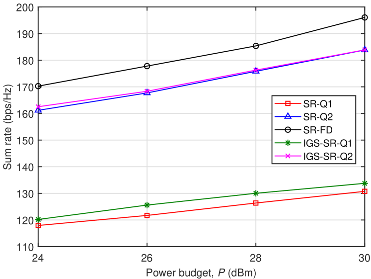
Figure 1: The SR vs. power budget $P$.

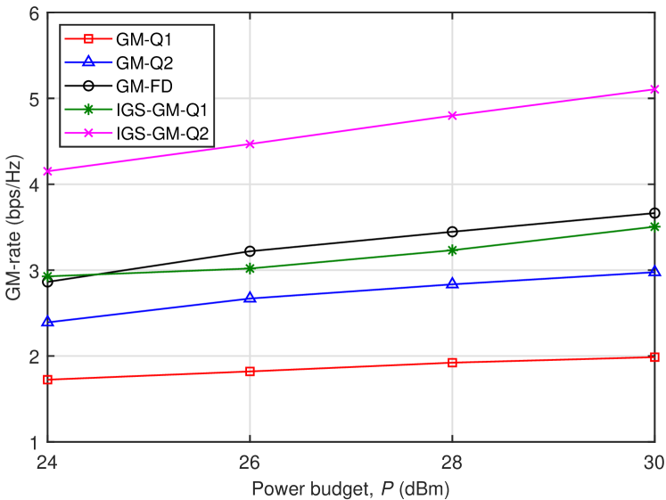
Figure 2: The GM-rate vs. power budget $P$.

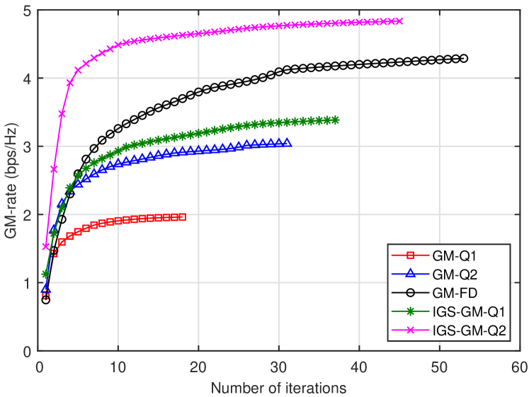
Figure 3: The GM-rate convergence of the GM-rate algorithms at $P=30$ dBm.

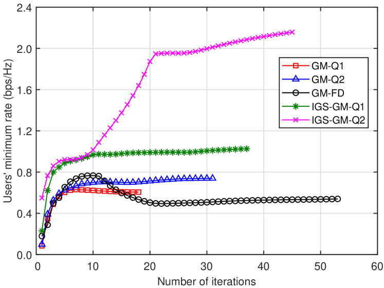
Figure 4: The MR convergence of the GM-rate algorithms at $P=30$ dBm.

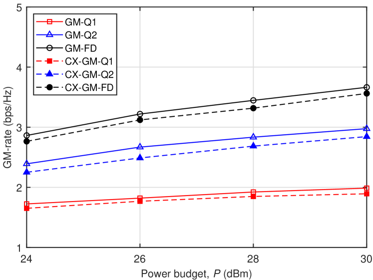
Figure 5: The GM-rate vs. power budget $P$ of the closed-form and convex-solver based algorithms.

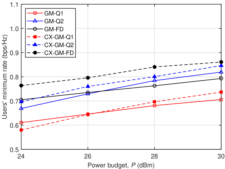
Figure 6: The MR vs. power budget $P$ of the closed-form and convex-solver based algorithms.

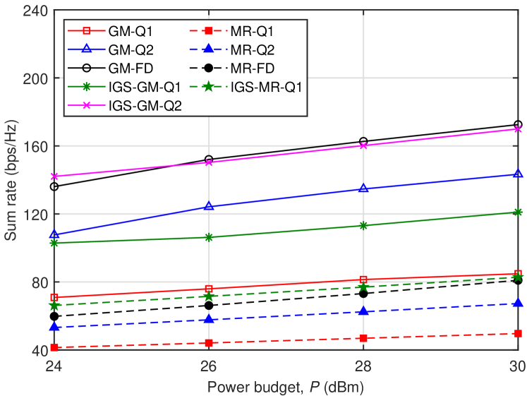
Figure 7: The SR vs. power budget $P$ by the GM-rate and MR algorithms.

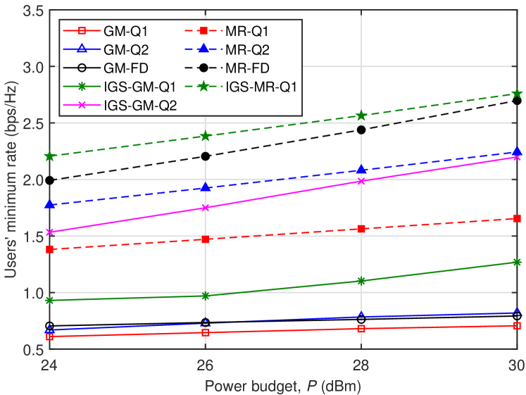
Figure 8: The MR vs. power budget $P$ by the GM-rate and MR algorithms.

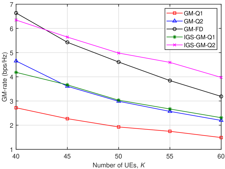
Figure 9: The GM-rate vs. the number $K$ of UEs.

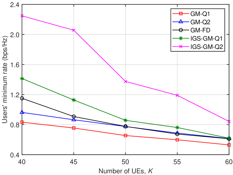
Figure 10: The MR vs. the number $K$ of UEs.

We use the following legends to specify the proposed implementation: MR-Q1/Q2 refer to the convex-solver based Alg. 1 with $Q=1$ (2D beamforming)/$Q=2$, while MR-FD refers to the baseline convex-solver based Alg. 4; SR-Q1/GM-Q1 and SR-Q2/GM-Q2 refer to the closed-form based Alg. 3 for SR/GM-rate maximization associated with $Q=1$ and $Q=2$, while SR/GM-FD refers to the baseline closed-form based Alg. 5 for SR/GM maximization; CX-GM-Q1/Q2 refers to the convex-solver based Alg. 2 for GM-rate maximization with $Q=1/Q=2$; IGS-MR-Q1 refers to the convex-solver based Alg. 6 for $Q=1$. Lastly, IGS-SR/GM-Q1/Q2 refer to the closed-form based IGS Alg. 7 for SR and GM-rate maximization associated with $Q=1/Q=2$.

We start by characterizing the SR maximization. Fig. 2 shows the SR vs. power budget $P$. One can see that the SR-FD achieves the highest SR, followed by SR-Q2 and IGS-SR-Q2. However, Table II shows that SR maximization results in many near-zero rates, and thus effectively disconnects many users. Therefore, the SR maximization is not applicable in multi-user scenarios. Thus, from now we focus our attention on simulating the MR and GM-rate maximization only with the following interesting outcomes: $(i)$ GM-rate maximization indeed achieves both good MR and SR, i.e. it provides an Pareto optimal solution for optimizing multi-objective MR and SR, while MR maximization sacrifices the SR to support the MR; $(ii)$ The closed-form based GM-Q1/Q2 performs similarly well to the convex-solver based CX-GM-Q1/Q2, but the computational complexity of the former is linear; $(iii)$ GM-Q2 already approaches GM-FD, and $(iv)$ IGS-GM-Q2 outperforms GM-FD.

Fig. 2 plots the GM-rate vs. power budget $P$. IGS-GM-Q1 gradually approaches the baseline GM-FD, while IGS-GM-Q2 significantly outperforms GM-FD. Fig. 4 shows the GM-rate convergence at $P=30$ dBm. GM-FD requires almost 50 iterations for convergence, because it has the largest numbers of decision variables. By contrast, GM-Q1 has the smallest number of decision variables, and it requires less than 20 iterations to achieve convergence. Fig. 4 shows the MR behaviour of the closed-form expression based GM-rate algorithms at $P=30$ dBm, where GM-Q1/Q2 tend to slightly sacrifice the MR for the sake of achieving a higher GM-rate, while GM-FD substantially reduces the MR to allow the GM-rate to be increased further. By contrast, IGS-GM-Q1/Q2 improve the MR along with the GM-rate. GM-FD and IGS-GM-Q2 require more iterations for convergence than the others, because the former has a large number of decision variables.

We compare the performances of the closed-form expression based and convex-solver based algorithms. Fig. 6 and Fig. 6 plot the GM-rate and MR achieved, which show that they perform similarly although the computational complexity of the former is very high compared to that of the latter.

Furthermore, we compare the SR and MR achieved by MR and GM-rate maximization. Fig. 8 shows that the GM-rate maximization achieves higher SR than MR maximization. Furthermore, GM-FD and IGS-GM-Q2 achieve the highest SR, followed by GM-Q2 and IGS-GM-Q1. Also IGS-MR-Q1 achives a better SR than MR-Q2. Fig. 8, which plots the MRs achieved, shows that MR maximization indeed achieves better MR than the GM-rate maximization, while IGS-GM-Q2 barely catches up with GM-Q2 at $P=30$ dBm. It is not surprising that IGS-MR-Q1 achieves the best MR and it even performs better than FD-MR does. Fig. 4, Fig. 4, Fig. 8, and Fig. 8 reveal that by iterating upon evaluating the GM-rate maximization, one can satisfy the MR required, while maintaining a good SR. Hence, for obtaining a reasonable MR at a moderate computational overhead, we prefer the closed-form expression based GM-rate algorithms, instead of the convex-solver based MR algorithms.

Table III provides the MR and SR achieved by the proposed algorithms at $P=30$ dBm for a particular channel generation, which confirms that the GM-rate maximization associated with linear computational complexity achieves similar MRs to that of direct MR maximization, but the latter imposes high-order polynomially increasing complexity. While the former succeeds in maintaining a very good SR, the latter has to sacrifice the SR in favor of maximizing the MR.

For more qualitative analysis, Table IV shows the min-rate/max-rate patterns and Jain’s fairness index of the user rate, which is defined as $\frac{(\sum_{k=1}^{K}r_{k})^{2}}{K\sum_{k=1}^{K}r_{k}^{2}}$ [38], at $P=30$ dBm. The IGS beamformers achieve higher min-rate to max-rate ratio and higher Jain’s fairness index, demonstrating that they promise fairer rate distributions among the UEs than others.

To substantiate the superior capability of GM-rate maximization in terms of efficient beamforming at identical transmit powers at the antennas, we provide Table V for the min-power to max-power ratio and for Jain’s fairness index of the antenna transmit power distributions. Observe in Table V that the antenna transmit power distributions achieved by the sum of one or two outer product-based beamformers are similar to that achieved by FD.

TABLE IV: Min-rate/max-rate and Jain’s fairness index of user rate by the GM-rate algorithms at $P=30$ dBm and $K=30$

	GM-Q1	GM-Q2	GM-FD	IGS-GM-Q1	IGS-GM-Q2
Min-rate/max-rate	0.0547	0.0486	0.0459	0.1395	0.1532
Jain’s fairness index	0.4725	0.4944	0.5561	0.7788	0.7923

TABLE V: Min-power/max-power and Jain’s fairness index of antenna power by the GM-rate algorithms at $P=30$ dBm and $K=30$

	GM-Q1	GM-Q2	GM-FD	IGS-GM-Q1	IGS-GM-Q2
Min-power/max-power	0.1922	0.2008	0.1873	0.1512	0.1865
Jain’s fairness index	0.8195	0.8148	0.7949	0.7946	0.7985

TABLE VI: Min-rate/max-rate and Jain’s fairness index of user rate by the GM-rate algorithms at $P=40$ dBm and $K=60$

	GM-Q1	GM-Q2	GM-FD	IGS-GM-Q1	IGS-GM-Q2
Min-rate/max-rate	0.0313	0.0290	0.0291	0.0520	0.0506
Jain’s fairness index	0.3577	0.3768	0.4875	0.5862	0.6992

TABLE VII: Min-power/max-power and Jain’s fairness index of antenna power by the GM-rate algorithms at $P=40$ dBm and $K=60$

	GM-Q1	GM-Q2	GM-FD	IGS-GM-Q1	IGS-GM-Q2
Min-power/max-power	0.1717	0.1883	0.2051	0.1332	0.1915
Jain’s fairness index	0.8019	0.8165	0.8085	0.7989	0.8300

We now further evaluate the performance of the GM-rate algorithms for larger numbers of UEs in the scenario of a $12\times 12$ URA at the BS. In the following simulations, more UEs are randomly placed in a cell with a radius of 500 meters. The transmit power budget is fixed at 40 dBm.

Fig. 10 plots the GM-rate vs. the number $K$ of UEs. IGS-GM-Q2 achieves the highest GM-rate when serving more UEs. Fig. 10, which plots the MR vs. the number $K$ of UEs, shows that IGS-GM-Q2 is also capable of reaching significantly higher MR than the others. Furthermore, IGS-GM-Q1 outperforms FD at smaller number of UEs. When the number of UEs increases to $K=60$, the MR achieved by GM-FD, IGS-GM-Q1, and GM-Q2 are getting close to each other.

The min-rate/max-rate patterns and Jain’s fairness index of the user rate at $K=60$ are also included in Table VI. We can see that the IGS-based algorithms are capable of reaching fairer user rate distributions even when serving a large number of UEs.

According to the min-power to max-power ratio and to Jain’s fairness index provided in Table VII, we observe that the antenna transmit power distributions achieved by the sum of one or two outer product-based beamformers are similar to that attained by FD. Table VII follows a similar trend to Table V provided for an $8\times 8$ URA.

VI Conclusions

A suite of FD m-MIMO systems was conceived for a base station employing $M\times M$-URAs in the downlink to support multiple users. We proposed a low-complexity class of beamformers, which are represented by the sums of outer products of $M$-dimensional azimuth and $M$-dimensional elevation beamformers. We have developed low-complexity algorithms for maximizing the SR, MR and GM-rate and showed that the sums of two outer products associated with the design complexity order of $M$ perform similarly to the baseline FD beamformer having the excessive design complexity order of $M^{2}$. Furthermore, the scheme relying on the sum of two outer products in improper Gaussian signaling succeeds in outperforming the baseline FD beamformer.

References

• [1] Y.-H. Nam et al., “Full-dimension MIMO (FD-MIMO) for next generation cellular technology,” IEEE Commun. Mag., vol. 51, pp. 172–179, Jun. 2013.
• [2] Y. Kim et al., “Full dimension mimo (FD-MIMO): the next evolution of MIMO in LTE systems,” IEEE Wirel. Commun., vol. 21, pp. 26–33, Apr. 2014.
• [3] H. Ji et al., “Overview of full-dimension MIMO in LTE-advanced pro,” IEEE Commun. Mag., vol. 55, pp. 176–184, Feb 2017.
• [4] B. Mondal et al., “3D channel model in 3GPP,” IEEE Commun. Mag., vol. 53, pp. 16–23, Mar. 2015.
• [5] X. Li, S. Jin, X. Gao, and R. W. Heath, “Three-dimensional beamforming for large-scale FD-MIMO systems exploiting statistical channel state information,” IEEE Trans. Vehic. Tech., vol. 65, pp. 8992–9005, Nov. 2016.
• [6] W. Liu, Z. Wang, C. Sun, S. Chen, and L. Hanzo, “Structured non-uniformly spaced rectangular antenna array design for FD-MIMO systems,” IEEE Trans. Wirel. Commun., vol. 16, pp. 3252–3265, May 2017.
• [7] Q.-U.-A. Nadeem, A. Kammoun, M. Debbah, and M.-S. Alouini, “Design of 5G full dimension massive MIMO systems,” IEEE Trans. Commun., vol. 66, pp. 726–740, Feb. 2018.
• [8] Q.-U.-A. Nadeem, A. Kammoun, and M.-S. Alouini, “Elevation beamforming with full dimension MIMO architectures in 5G systems: A tutorial,” IEEE Commun. Surv. Tut., vol. 21, no. 4, pp. 3238–3273, 2019.
• [9] X. Li, Z. Liu, N. Qin, and S. Jin, “FFR based joint 3D beamforming interference coordination for multi-cell FD-MIMO downlink transmission systems”,” IEEE Trans. Vehic. Techn., vol. 69, pp. 3105–3118, Mar. 2020.
• [10] L. D. Nguyen, H. D. Tuan, T. Q. Duong, and H. V. Poor, “Multi-user regularized zero forcing beamforming,” IEEE Trans. Signal Process., vol. 67, pp. 2839–2853, Jun. 2019.
• [11] H. Yu, H. D. Tuan, A. A. Nasir, T. Q. Duong, and L. Hanzo, “Improper Gaussian signaling for computationally tractable energy and information beamforming,” IEEE Trans. Veh. Techn., vol. 69, pp. 13990–13995, Nov. 2020.
• [12] L. D. Nguyen, H. D. Tuan, T. Q. Duong, H. V. Poor, and L. Hanzo, “Energy-efficient multi-cell massive MIMO subject to minimum user-rate constraints,” IEEE Trans. Commun., vol. 69, pp. 914–928, Feb. 2021.
• [13] D. Ying, F. W. Vook, T. A. Thomas, D. J. Love, and A. Ghosh, “Kronecker product correlation model and limited feedback codebook design in a 3D channel model,” in Proc. 2014 IEEE Inter. Conf. Commun. (ICC), pp. 5865–5870, 2014.
• [14] A. Alkhateeb, G. Leus, and R. W. Heath, “Multi-layer precoding: A potential solution for full-dimensional massive MIMO systems,” IEEE Trans. Wirel. Commun., vol. 16, pp. 5810–5824, Mar. 2017.
• [15] J. Kang, O. Simeone, J. Kang, and S. Shamai, “Layered downlink precoding for C-RAN systems with full dimensional MIMO,” IEEE Trans. Vehic. Techn., vol. 66, pp. 2170–2182, Mar. 2017.
• [16] Z. Wang, W. Liu, C. Qian, S. Chen, and L. Hanzo, “Two-dimensional precoding for 3-D massive MIMO,” IEEE Trans. Vehic. Techn., vol. 66, pp. 5488–5493, June 2017.
• [17] Y. Song, C. Liu, W. Wang, N. Cheng, M. Wang, W. Zhuang, and X. Shen, “Domain selective precoding in 3-D massive MIMO systems,” IEEE J. Select. Topics Signal Process., vol. 13, pp. 1103–1117, May 2019.
• [18] H. H. M. Tam, H. D. Tuan, and D. T. Ngo, “Successive convex quadratic programming for quality-of-service management in full-duplex MU-MIMO multicell networks,” IEEE Trans. Commun., vol. 64, pp. 2340–2353, June 2016.
• [19] A. A. Nasir, H. D. Tuan, T. Q. Duong, and H. V. Poor, “Secrecy rate beamforming for multicell networks with information and energy harvesting,” IEEE Trans. Signal Process., vol. 65, no. 3, pp. 677–689, 2017.
• [20] H. Yu, H. D. Tuan, A. A. Nasir, T. Q. Duong, and H. V. Poor, “Joint design of reconfigurable intelligent surfaces and transmit beamforming under proper and improper Gaussian signaling,” IEEE J. Sel. Areas Commun., vol. 38, pp. 2589–2603, Nov. 2020.
• [21] H. Yu, H. D. Tuan, E. Dutkiewicz, H. V. Poor, and L. Hanzo, “Maximizing the geometric mean of user-rates to improve rate-fairness: Proper vs. improper Gaussian signaling,” IEEE Trans. Wirel. Commun., vol. 21, no. 1, pp. 295–309, 2022.
• [22] W. Zhu, H. D. Tuan, E. Dutkiewicz, and L. Hanzo, “Collaborative beamforming aided fog radio access networks,” IEEE Trans. Veh. Techn., vol. 71, pp. 7805–7820, Jul. 2022.
• [23] A. A. Nasir, H. D. Tuan, E. Dutkiewicz, and L. Hanzo, “Finite-resolution digital beamforming for multi-user millimeter-wave networks,” IEEE Trans. Veh. Techn., vol. 71, Sept. 2022.
• [24] A. A. Nasir, H. D. Tuan, E. Dutkiewicz, H. V. Poor, and L. Hanzo, “Low-resolution RIS-aided multi-user MIMO signaling,” IEEE Trans. Commun., vol. 70, pp. 6517–6531, Oct. 2022.
• [25] H. Tuy and H. D. Tuan, “Generalized S-lemma and strong duality in nonconvex quadratic programming,” J. of Global Optimization, vol. 56, pp. 1045–1072, 2013.
• [26] H. Tuy, Convex Analysis and Global Optimization (second edition). Springer International, 2017.
• [27] C. Hellings, M. Joham, and W. Utschick, “QoS feasibility in MIMO broadcast channels with widely linear transceivers,” IEEE Signal Process. Lett., vol. 20, pp. 1134–1137, Nov. 2013.
• [28] Y. Zeng, C. M. Yetis, E. Gunawan, Y. L. Guan, and R. Zhang, “Transmit optimization with improper Gaussian signaling for interference channels,” IEEE Trans. Signal Process., vol. 61, pp. 2899–2913, Jun. 2013.
• [29] S. Lagen, A. Agustin, and J. Vidal, “On the superiority of improper Gaussian signaling in wireless interference MIMO scenarios,” IEEE Trans. Commun., vol. 64, pp. 3350–3368, Aug. 2016.
• [30] A. A. Nasir, H. D. Tuan, T. Q. Duong, and H. V. Poor, “Improper Gaussian signaling for broadcast interference networks,” IEEE Signal Process. Lett., vol. 26, pp. 808–812, Jun. 2019.
• [31] H. D. Tuan, A. A. Nasir, H. H. Nguyen, T. Q. Duong, and H. V. Poor, “Non-orthogonal multiple access with improper Gaussian signaling,” IEEE J. Selec. Topics Signal Process., vol. 13, pp. 496–507, Mar. 2019.
• [32] U. Rashid, H. D. Tuan, and H. H. Nguyen, “Relay beamforming designs in multi-user wireless relay networks based on throughput maximin optimization,” IEEE Trans. Commun., vol. 61, pp. 1739–1749, May 2013.
• [33] T. L. Marzetta, E. G. Larsson, H. Yang, and H. Q. Ngo, Fundmentals of Massive MIMO. UK.: Cambridge Univ. Press, 2016.
• [34] D. Peaucelle, D. Henrion, and Y. Labit, “Users guide for SeDuMi interface 1.03,” 2002.
• [35] T. M. Cover and J. A. Thomas, Elements of Information Theory (second edition). John Wileys & Sons, 2006.
• [36] A. Adhikary, J. Nam, J. Ahn, and G. Caire, “Joint spatial division and multiplexing-the large-scale array regime,” IEEE Trans. Inf. Theory, vol. 59, pp. 6441–6463, Oct. 2013.
• [37] 3GPP, “Study on channel model for frequencies from 0.5 to 100 GHz,” 3rd Generation Partnership Project (3GPP), Sophia Antipolis Cedex, France, Tech. Rep. TR 38.901 (V14.2.0), Sep. 2017. [Online]. Available: http:// www.3gpp.org/.
• [38] R. Jain, D.-M. Chiu, and W. R. Hawe, “A quantitative measure of fairness and discrimination for resource allocation in shared computer systems,” Digital Equipment, Tech. Rep. DEC-TR-301, Sept. 1984.