Distributed Planning with Asynchronous Execution with Local Navigation for Multi-agent Pickup and Delivery Problem

Abstract.

We propose a distributed planning method with asynchronous execution for multi-agent pickup and delivery (MAPD) problems for environments with occasional delays in agents’ activities and flexible endpoints. MAPD is a crucial problem framework with many applications; however, most existing studies assume ideal agent behaviors and environments, such as a fixed speed of agents, synchronized movements, and a well-designed environment with many short detours for multiple agents to perform tasks easily. However, such an environment is often infeasible; for example, the moving speed of agents may be affected by weather and floor conditions and is often prone to delays. The proposed method can relax some infeasible conditions to apply MAPD in more realistic environments by allowing fluctuated speed in agents’ actions and flexible working locations (endpoints). Our experiments showed that our method enables agents to perform MAPD in such an environment efficiently, compared to the baseline methods. We also analyzed the behaviors of agents using our method and discuss the limitations.

1. Introduction

Multi-agent path-finding (MAPF), in which multiple agents move to their destinations by avoiding collisions, is an important abstract problem that arises in many applications, such as robotics and games Salzman and Stern (2020); Jennings et al. (1997); Pěchouček et al. (2006). For example, in an automated warehouse, the robots (carrier agents) move to the pickup locations, load materials, and deliver them to their respective unloading locations, by repeatedly assigning new tasks to agents consecutively. This type of application in which MAPF problems are iteratively solved is formulated as a multi-agent pickup-and-delivery (MAPD) problem Ma et al. (2017). Therefore, the objective of MAPD is that agents repeatedly move to their respective task endpoints, which are pickup and delivery locations Ma et al. (2017), without collisions.

However, complex and restrictive environments may reduce efficiency and hence increase the chances of collisions. Furthermore, uncertainties often exist in practice. For example, The occasional delays in the movements of some agents will affect the plans of others. Consequently, many agents cannot move according to their plans as previously determined. In such a case, these agents have to replan their paths to avoid collisions. However, replanning requires considerable computational cost with an increasing number of agents when using centralized methods or when assuming synchronized movement with decentralized control. Meanwhile, we envisioned an application for robotic material transfer in a construction site and a disaster area and such uncertainty is not preventable. Thus, we focused on a distributed planning-and-executing method wherein agents generate their plans individually and move to their destinations interacting only with the local agents involved to address the negative effects of delays and resource conflicts. Although distributed planning for MAPD has some issues to be addressed, such as completeness and avoidance of live-/dead-lock, we think that a distributed planning method is preferable because of their desirable characteristics, such as robustness, scalability, and reconfigurability Yan et al. (2013).

Although there are several studies on planning and execution in MAPF and MAPD, most studies assumed grid-like environments, such as an automated warehouse wherein (1) there are many endpoints more than agents and (2) the agents move at a constant speed and move synchronously Ma et al. (2017). Moreover, these conventional methods require a well-formed infrastructure conditions (WFI conditions) Čáp et al. (2015). For example, in the holding task endpoint (HTE) Ma et al. (2017), any path connecting a pair of endpoints does not traverse any other endpoints. These types of requirements can be easily satisfied in a simple grid-like environment, but are not feasible in our target applications. For example, at a construction site, heavy-duty robots transport heavy building materials weighing 500 kg and above between storage locations, specific work locations, and/or elevators that carry them to other floors, during the night for the next day’s work; the number of these endpoints (i.e., storage and working locations) is not large. Therefore, several agents are likely to move to a few specific endpoints as their destinations simultaneously, but should not collide with each other. Furthermore, (1) owing to a variety of working locations, the WFI conditions cannot necessarily be met, and (2) agents cannot often move at a constant speed because of various reasons, such as temperature, humidity, wet floor, slopes/small steps, and sensor errors.

Our contribution is twofold. First, we introduced a problem of MAPD with fluctuated movement speed (MAPDFS), which is an abstraction of our target application that involves material transport tasks by multiple robots at a construction site, considering the characteristics discussed above, such as a smaller number of endpoints, and uncertainty in agent’s movement speed.

Second, we presented a novel distributed planning with an asynchronous execution method for MAPD problems. Its features are low-cost planning without considering the plans of other agents and the adjacent movements of multiple agents, based on possible conflict detection in an environment described by the graph consisting of several bi-connected components with small tree-structured areas. We introduced into MAPD two types of agents: carrier agents, simply called agents, that carry materials while planning paths with ignoring other agents, and node agents that manage the corresponding nodes in the graph and detect the possibility of conflicts by communicating only with the neighboring nodes. After a carrier agent plans a path, it communicates with the node agent managing the current node, and then the node agent requests the next node agent to reserve the node. Depending on the response, the current node agent suggests to the carrier agent that it can move to the next node, should move to another node (i.e., taking a detour) or should wait for a while at the current node. Then, it moves/waits asynchronously without considering other agents. Moreover, when it moves to another node that is not in the current plan, it replans another path, ignoring other agents.

The basic idea behind the ignorance of other agents is the fact that detailed planning with rigorous execution will easily become unavailable in a real environment that may have uncertainty. Conversely, to reduce collisions, we introduced the orientation to the environment such that its main area can be observed as a strongly connected graph. Subsequently, the direct edges are used to navigate the agents based on the directions and eliminate head-on collisions and dead-/livelock, such as a roundabout. This may force agents to take detours; however, it simplifies the independent planning process, makes it easier to detect potential collisions, allows agents to delay/stop moving, and relaxes the WFI conditions with a small number of endpoints. These features are indispensable in real-world applications. We then experimentally evaluated the performance of the proposed method by comparing it with two baseline methods, rolling-horizon collision resolution (RHCR) Li et al. (2021) and HTE  Ma et al. (2017). We found that our proposed method outperformed the baseline methods in the environment that meets the conditions they require. We also showed that agents with our method can complete all tasks without collisions, despite occasional delays in agent speed and flexibility in locating the endpoints.

2. Related Work

Although finding collision-free paths is a basic requirement for MAPF/MAPD, it is known as an NP-hard problem Yu and LaValle (2013), which involves high computational costs. Therefore, several studies attempted to find sub-optional solutions by relaxing problems Barer et al. (2014); Boyarski et al. (2015); Felner et al. (2018).

MAPF is often integrated into MAPD by iterating path-finding using centralized planners Nguyen et al. (2017); Cohen et al. (2015); Huang et al. (2021); Liu et al. (2019). For example, Nguyen et al. Nguyen et al. (2017) solved task assignment and path-finding problems using answer set programming. Cohen, Uras, and Koenig Cohen et al. (2015) extended conflict-based search (CBS) Sharon et al. (2015) by adding a set of edges with the user-specified orientation, called highways, that provide collision-avoidance guidance by eliminating agents travel in the opposite direction. The highways also contribute to decreasing the runtimes and solution costs of the MAPF solver for autonomous robots in a warehouse. However, these centralized planners do not scale because of high computational and communication costs with an increasing number of agents. Our method can be considered a combination of highways and the distributed planning and execution because we also oriented edges (algorithmically) in environments to locally navigate agents.

Other sub-optimal centralized planning methods Švancara et al. (2019); Li et al. (2021); Wiktor et al. (2014) decompose iterative MAPFs into sequential path-planning problems in which a solver replans all paths at every timestep. Because these methods have computationally high costs, some studies attempted to improve scalability. Švancara et al. Švancara et al. (2019) considered an online MAPF in which new agent goals may be added dynamically and disappear at their goals. They then proposed the online independence detection algorithm for generating plans to reduce disruptions of existing plans. Li et al. Li et al. (2021) proposed RHCR in which agents find conflicts that occur in the $w$-timestep windows and replan paths every $h$ timesteps. However, if the environment is dense and crowded, many paths for other agents have to be checked to generate a collision-free path, resulting in high computational costs.

The decentralized planning of collision-free paths has also been studied Ma et al. (2017, 2019b); Wiktor et al. (2014); Okumura et al. (2019); Yamauchi et al. (2022). For example, Ma et al. Ma et al. (2017) proposed HTE, which is a prioritized path planning method wherein agents plan their paths consecutively and the new path is required to be collision-free with existing paths of other agents. The priority inheritance with back-tracking (PIBT) Okumura et al. (2019) focuses on the adjacent movements of multiple agents based on prioritized planning in a short time window. These methods require environmental conditions to guarantee the completeness of MAPD instances. HTE requires the WFI condition and PIBT requires that the environment is a bi-connected graph. Although these environmental conditions apply to some applications (e.g., MAPD in an automated warehouse), the environments of other applications (e.g., construction sites and some logistics sorting centers Wan et al. (2018)) cannot satisfy these conditions. Furthermore, agents are forced to synchronize movements in decentralized approaches such as these and thus cannot handle fluctuations in moving speed.

Meanwhile, we assumed that distributed approaches are more suitable in our applications because agents can move asynchronously and improve scalability and robustness. However, the methods from this approach are sometimes incomplete. For example, Wilt and Botea Wilt and Botea (2014) proposed a spatially distributed planner in which each controller agent manages a subarea and communicates with the adjacent controller confirming the transfer of a mobile unit to another subarea. However, this method is partially centralized to make it complete. Thus, its environmental condition is somewhat inflexible, and agents cannot move asynchronously. Miyashita, Yamauchi, and Sugawara Miyashita et al. (2022) proposed a distributed planning that enables agents to move asynchronously. Their method introduces two types of agents such as ours, carrier agents, which carry materials, and node agents, which manage the resource conflicts. However, their method is significantly complicated to implement. Our method takes a similar approach but is much simpler and low-cost, and agents can move effectively even in a crowded area.

3. Problem formulation

3.1. MAPD

In the MAPD problem, carrier agents, or simply agents load materials at specified locations, carry them to specified destinations, and unload them. Let $I=\{1,\cdots,n\}$ be the set of agents and $\mathcal{T}=\{\tau_{1},\cdots,\tau_{{|\mathcal{T}|}}\}$ be a set of tasks that should be completed by the agents. An environment is described by a connected graph $G=(V,E)$ that can be embedded into a two-dimensional space, where $V=\{v_{1},\cdots,v_{{|V|}}\}$ is a set of nodes corresponding to locations and $E$ is a set of edges corresponding to connections between two neighboring nodes. Our graph is constituted at a combination of indirect and direct edges, and hence the edge connecting $v_{j}$ and $v_{k}$ is denoted as either $(v_{j},v_{k})\in E$ for the indirect edge or $(v_{j}\shortrightarrow v_{k})\in E$ for the direct edge. Therefore, $(v_{j}\shortrightarrow v_{k})$ indicates the path through which agents can move only from $v_{j}$ to $v_{k}$, while agents can move to both directions between $v_{j}$ and $v_{k}$ on $(v_{j},v_{k})$. Note that we assume that agent $i$ cannot stop on an edge. Two agents collide only when they exist on a single node or traverse the same edge in opposite directions; this implies that a collision does not occur on the direct edge.

Task $\tau_{k}\in\mathcal{T}$ is specified by a tuple $\tau_{k}=(v_{k}^{l},v_{k}^{u},\mu_{k})$, where $\mu_{k}$ is the material to carry, $v_{k}^{l}$ is the pickup node where to load $\mu_{k}$, and $v_{k}^{u}$ is the destination node where to unload $\mu_{k}$. The nodes where agents load and unload materials are called task endpoints. We introduce discrete time $t\geq 0$, whose unit is timestep. When agent $i\in I$ is allocated task $\tau_{k}\in\mathcal{T}$ at time $t$, it individually plans to generate a path from node $v_{\it c}^{i}(t)$ to $v_{k}^{l}$ to load $\mu_{k}$ and a path from $v_{k}^{l}$ to $v_{k}^{u}$ to unload it, where $v_{\it c}^{i}(t)$ is the node on which $i$ is at $t$. Then, $i$ moves to $v_{k}^{l}$ and $v_{k}^{u}$ along the paths and load/unload $\mu_{k}$. If a collision is possible, $i$ has to modify the path to avoid it.

Initially ($t=0$), agent $i$ starts from its own parking node, $v_{i}^{\it pk}$ ($=v_{\it c}^{i}(0)$), and then begins to execute the given tasks in $\mathcal{T}$ with other agents. An agent can move to one of neighboring nodes in $T_{\it mv}$ timesteps if possible, but may need longer time $T_{\it lu}$ ($\geq T_{\it mv}$) for loading/unloading. It can also wait at a node for any timesteps. We may assume fluctuations in the agent’s speed; that is, it occasionally takes longer than $T_{\it mv}$ to move to a neighboring node. When $i$ has completed the current task, one element in $\mathcal{T}$ is allocated to it. When $\mathcal{T}=\varnothing$, $i$ returns to its parking node. We define that an endpoint is a task endpoint or a parking node.

3.2. Required Environmental Conditions

We assume our environment $G=(V,E)$ consists of some bi-connected components with small trees. We define it more formally. Let $G$ be a undirected graph and $G^{\prime}=(V^{\prime},E^{\prime})$ be a subgraph of $G$ associated with $V^{\prime}\subset V$, that is, $(v_{1},v_{2})\in E^{\prime}$ iff $v_{1},v_{2}\in V^{\prime}$ and $(v_{1},v_{2})\in E$.

Definition .

(Bi-connected component)

• $G^{\prime}$ is a bi-connected subgraph of $G$ iff, for $\forall v_{1},v_{2}\in V^{\prime}$, $G^{\prime}$ contains a cycle connected $v_{1}$ and $v_{2}$.

• Bi-connected subgraph $G^{\prime}$ of $G$ is a maximal if $\not\exists v\in V\setminus V^{\prime}$ s.t. the subgraph of $G$ associated with $V^{\prime}\cup\{v\}$ is the bi-connected subgraph.

• A maximal bi-connected subgraph of $G$ is called a bi-connected component.

Let $G_{1},\dots,G_{K}$ be all bi-connected components of $G$. We denote $G_{k}=(V_{k},E_{k})$. We call $G_{\it main}=G_{1}\cup\dots\cup G_{K}$ the main area of $G$, where we define the union of graphs as $G_{k}\cup G_{k^{\prime}}=(V_{k}\cup V_{k^{\prime}},E_{k}\cup E_{k^{\prime}})$. We assume that our environment $G$ holds the following structural (SC) and agent (AC) conditions:

• $G_{\it main}$ is a connected graph.

• For $\forall v\in V\setminus V_{\it main}$, $v$ is a node in one of $L$ tree-structured subgraphs of $G$, $G_{\it tree}^{1},\dots,G_{\it tree}^{L}$, and for $1\leq k\leq L$, $G_{\it tree}^{k}\cap G_{\it main}$ is a singleton whose element is the root node of $G_{\it tree}^{k}$.

• Parking nodes are end nodes in tree-structured subgraphs that have no task endpoints.

• Agents are at least two fewer than the nodes in the main area, ${|I|}\leq{|G_{\it main}|}-2$, but we suggest that agents be fewer than half of ${|G_{\it main}|}$ for efficiency. This topic will be discussed later.

We denote the set of all root nodes as $G_{\it root}=(G_{\it tree}^{1}\cup\dots\cup G_{\it tree}^{L})\cap G_{\it main}$. By defining marginal zone as $G_{\it mar}=G_{\it tree}^{1}\cup\dots\cup G_{\it tree}^{L}\setminus G_{\it root}$, $G=G_{\it main}\cup G_{\it mar}$ is evidently a disjoint union. Then, the following proposition is true.

Proposition 0.

Suppose that $G_{\it main}=G_{1}\cup\dots\cup G_{K}$ is connected graph and $G_{k}$ is the bi-connected component. If $V_{k}\cap V_{k^{\prime}}\not=\varnothing$, the $V_{k}\cap V_{k^{\prime}}$ is a singleton.

Proof.

If $V_{k}\cap V_{k^{\prime}}$ has two nodes, $V_{k}\cup V_{k^{\prime}}$ is bi-connected; thus, $V_{k}$ and $V_{k^{\prime}}$ are not bi-connected components, and this is a contradiction (the detailed proof is provided in Appendix). ∎

We can set a task endpoint to any nodes in $G$ subject to Condition SC3 If an agent loads/unloads a material on the nodes in the main area, the movement of other agents may temporarily impeded. However, because working places are possible anywhere on a construction site, we believe that it is inevitable and agents should carry the required materials to such places.

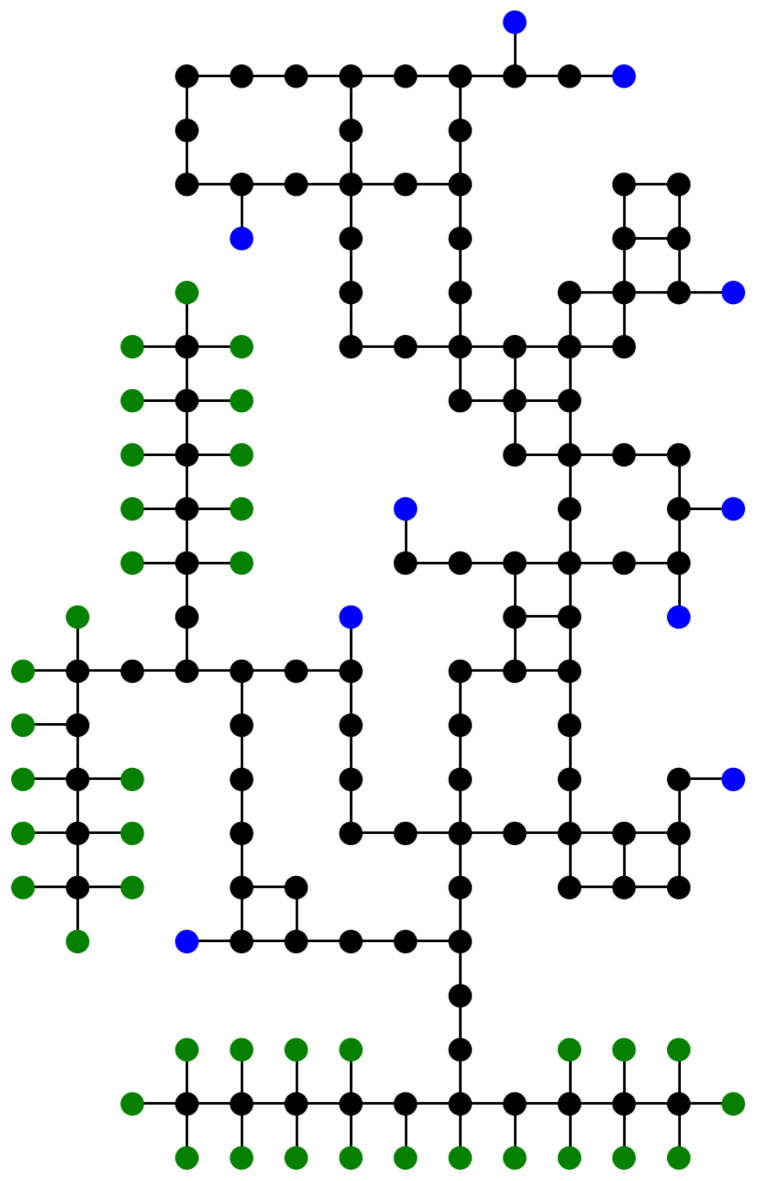
(a) Environment 1 (Env. 1)

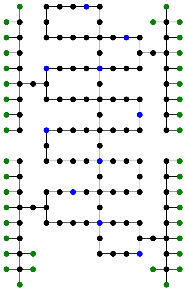
(b) Environment 2 (Env. 2)

Figure 1. Example environments.

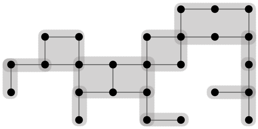
(a) Graph structure.

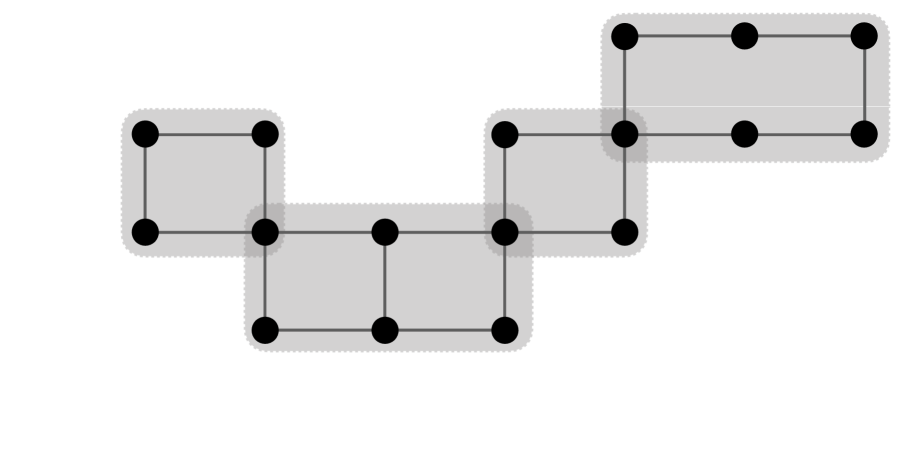
(b) Main area.

Figure 2. Example environment.

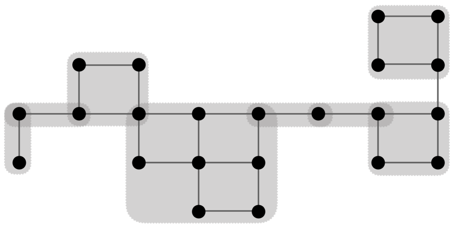
(a) Graph

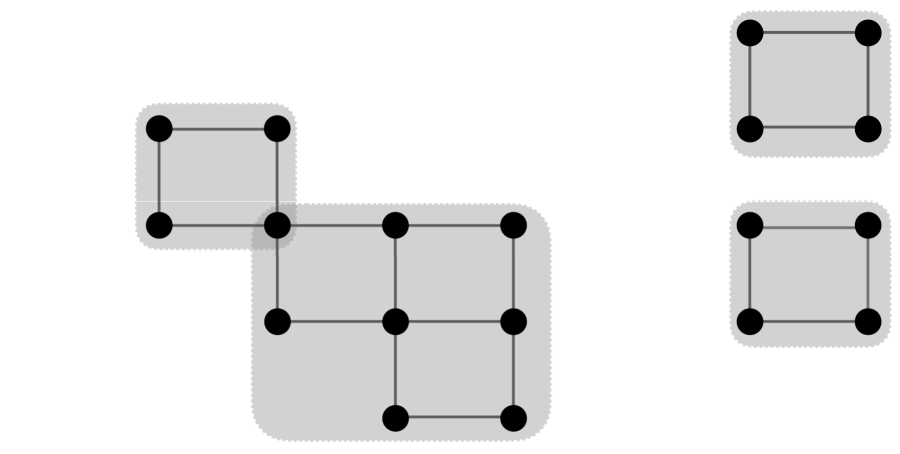
(b) Main area is disconnected.

Figure 3. Graph that does not hold the conditions.

The example of our environment is shown in Fig. 1, where (forty) green dots are parking nodes for individual agents and blue dots are task endpoints (i.e., loading and unloading locations). Another example is shown in Fig. 2; Fig. 2 shows the environment, and Fig. 2 is its main area. Fig. 3 shows the graph that does not meet our conditions: actually, the main area is not connected (Fig. 3), and some nodes in $G_{\it mar}$ are not nodes in trees.

4. Proposed method

One feature of the proposed algorithm is simple planning by ignoring the other agents’ current plans. Instead, for $\forall v\in V_{\it main}$, we introduce the node agent, which manages the resource of $v$ and detects the possibility of conflict, that is, collisions between agents. While a (carrier) agent communicates only with the current node agent that manages the resource of the current node, a node agent communicates with the neighboring node agents and checks the possibility of movement of the agent on itself. The node agent is also represented hereinafter by $v$. A carrier agent generates a path, which is a sequence of nodes to the destination independently and asynchronously, and moves to the next node based on the path while making sure that another agent does not stay at the next node or move toward it by asking the current node agent.

Note that node agents are not necessarily located on the corresponding nodes because they only manage the reservation of the corresponding nodes. Thus, they can run on a single machine, on different servers in a cloud, or on intelligent sensors near the locations. The only requirement is that the node agent should be able to communicate with the node agents that manage the neighboring nodes and with the carrier agent that is currently reserving the node.

4.1. Orienting Graphs with Reachability

Our basic idea is to introduce a strong orientation in the main area to prevent crossing the same edge, particularly moving in opposite directions along a long straight path consisting of multiple edges. This may result in detours, but conversely allows consistent structural direction for the flows of movements. Thus, agents can avoid collisions with only local information and resource allocation, address travel delays, or sudden stops in an opportunistic manner. This also eliminates the need for costly planning considering other agents’ paths and negotiation to avoid collisions.

First, we introduce the basic concepts related to graph theory.

Definition .

A directed graph is a strongly connected iff any pair of nodes has paths in both directions between them.

Definition .

An edge in an undirected connected graph is called a bridge iff the graph is not connected anymore if it is eliminated.

Evidently, our main area $G_{\it main}$, is bridgeless (or 2-edge connected) and connected. Then, the following theorem is known as the one-way street theorem Robbins (1939). A bridgeless connected undirected graph can be made into a strongly connected graph by consistently orienting (and vice versa).

Several efficient algorithms (linear and $\log{|E|}$) to orient a bridgeless connected undirected graph to make it strongly connected have been proposed Atallah (1984); Dijkstra (1976); Tarjan (1972). We orient $G_{\it main}$ using one of these algorithms. Note that edges in $G_{\it mar}$ remain undirected, which means bi-directional edges that an agent travels in both directions. An example of the oriented environment of Fig. 2 is shown in Fig. 4.

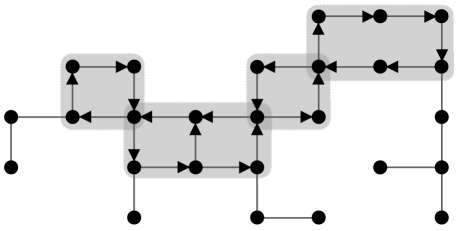
Figure 4. Example of orienting graphs.

4.2. Behavior of Carrier Agents

We assume that the environment $G$ has already been oriented, as described in the previous section. When task $\tau_{k}=(v_{p}^{k},v_{d}^{k},\mu^{k})$, is allocated to carrier agent $i$, $i$ will move to its load location $v_{p}^{k}$, and to its unload location $v_{d}^{k}$. Therefore, $i$ sets the destination node, $v_{\it dst}\in V$, to $v_{p}^{k}$ or $v_{d}^{k}$ in $\tau_{k}$, depending on the phase of the task progress and then generates the shortest path $p_{i}$ (or appropriate path from another perspective) from the current node $v_{\it c}^{i}$, to $v_{\it dst}$, using a conventional method (e.g., $A^{*}$-search) in the (partly) directed graph $G$. Herein, we define a path $p$ from node $v$ to node $v^{\prime}$ as the sequence of nodes $p=(v_{0}^{p},v_{1}^{p},\dots v_{|p|}^{p})$, where $v_{0}^{p}=v$ and $v_{k}^{p}=v^{\prime}$ and $v_{k-1}^{p}$ and $v_{k}^{p}$ are connected by edge $(v_{k-1}^{p},v_{k}^{p})$ or $(v_{k-1}^{p}\shortrightarrow v_{k}^{p})$. Note that, unlike other methods for MAPD, we can generate a path by ignoring time information, that is, when agents arrive and leave nodes. After generating path $p_{i}$, $i$ attempts moving to $v_{\it dst}$ in line with $p_{i}$.

We denote the current node of agent $i$ at $t$ by $v_{\it c}^{i}(t)$. Agent $i$ has the facilitator node agent (or simply, facilitator), $v_{\it Fcl}^{i}(t)\in V_{\it main}$, which is identical to the current node $v_{\it Fcl}^{i}(t)=v_{\it c}^{i}(t)$ if $v_{\it c}^{i}(t)\in V_{\it main}$, and if $i$ is in a tree (i.e., $v_{\it c}^{i}(t){\color[rgb]{0,0.6,0}}\in G_{\it tree}^{k}$), its facilitator node is set to the root node, $v_{\it Fcl}^{i}(t)\in G_{\it tree}^{k}\cap G_{\it main}$. If $v_{\it c}^{i}(t)$ and the next node $v_{\it next}^{i}\in p_{i}$ are not in $V_{\it main}$, $i$ moves to $v_{\it next}^{i}$ without confirmation. Otherwise (i.e., if $v_{\it c}^{i}(t)\in V_{\it main}$ or $v_{\it next}^{i}\in V_{\it main}$), before $i$ at $v_{\it c}^{i}(t)$ moves to next node $v_{\it next}^{i}\in p_{i}$, $i$ sends a request message to node agent $v_{\it Fcl}^{i}$ with $p_{i}$ to reserve $v_{\it next}^{i}$. Then, it will receive its reply from $v_{\it Fcl}^{i}$. If it is an acceptance message, $i$ leaves the current node for $v_{\it next}^{i}$ at $t+1$ and releases the reservation for $v_{\it c}^{i}(t)$. Note that it may take some time $T_{\it mv}\geq 1$ to reach $v_{\it next}^{i}$; however, we assume that $v_{\it c}^{i}(t+1)=v_{\it next}^{i}$ until $i$ leaves there. It also means that their activities are asynchronous if $T_{\it mv}>1$; that is, when an agent starts leaving the current node, other agents may already be in the middle of edges. After $i$ reaches the next node, $i$ attempts to reserve the next node $v_{\it next}^{i}$ based on plan $p_{i}$.

Meanwhile, if $i$ receives a denial message from node agent $v_{\it Fcl}^{i}$ for reserving $v_{\it next}^{i}$, the message contains the suggestion of movement (SOM), wait (i.e., waiting for a while) or detour with another next node in $V_{\it main}$ (i.e., taking a detour) which neighbors $v_{\it c}^{i}(t)$. When the SOM is detour, $i$ leaves for the specified next node and generates another (shortest) path $p_{i}$ from that node to the destination using a conventional algorithm without considering the planned paths of other agents. Note that it is probable that the generated new path contains $v_{\it next}^{i}$ that was denied; however, all edges in $G_{\it main}$ are directed, thus $i$ should take a detour to return to $v_{\it next}^{i}$, therefore, its surrounding situation becomes different.

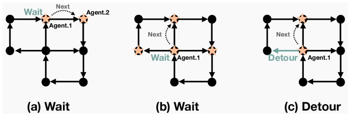
Figure 5. Example of the denial message with SOM.

4.3. Node Agent Behavior for Conflict Detection

Node agent $v\in V_{\it main}$ manages the reservation of the corresponding node $v$ for the staying (carrier) agent $i$ at $v$ as the facilitator. It confirms whether $i$ can move to the next node by communicating with the neighboring node to determine the possibility of a collision. This implies that more than two agents $i,j\in I$ attempt to reserve the same node simultaneously, but we assume that the node agent reads them from its message queue one by one.

When node agent $v$ receives a request message to move to neighboring node $v_{\it next}^{i}\in V_{\it main}$ from agent $i$ on $v=v_{\it c}^{i}(t)$, $v$ asks the vacancy to node agent $v_{\it next}^{i}$ by sending a reservation message. If $v_{\it next}^{i}$ is reserved by no other agent at $t+1$, $v_{\it next}^{i}$ reserves its resource for $i$ and $v_{\it next}^{i}$ sends the acceptance message $v$ and it is forwarded to $i$. If $v_{\it next}^{i}$ is already reserved at $t+1$ or another agent $j$ on $v_{\it next}^{i}$ is not decided to move to $v_{\it next}^{j}$ at $t+1$, facilitator $v$ forwards a denial message from $v_{\it next}^{i}$ to $i$ with the possible action label, which is among the following SOMs:

Wait::

Node agent $v$ suggests for $i$ to extend the current stay until $t+1$ (thus the extension is not necessarily $T_{\it mv}$). This is always possible because $v$ accepts the reservation request from another agent only after $i$ has reserved the next node.

Detour::

Suppose that $v$ has multiple outward-direct edges. $v$ sends the reservation message to the neighboring node, consecutively, except $v_{\it next}^{i}$, and if one of them $\tilde{v}_{\it next}^{i}$ accepts it, $v$ sends the denial message with detour and the reserved node $\tilde{v}_{\it next}^{i}$ for $i$.

Node agent $v$ should select which SOM, wait or detour, depending on the situation. Both SOMs have their pros and cons; the wait SOM may block other agents, whereas the detour SOM may force $i$ to take a detour. However, in our experiments, node agent $v$ attempted to send the detour, and when it was not possible, it sent wait, because ensuring that the agent’s flow is not disrupted is effective in the efficient execution of tasks, particularly in a crowded situation. Examples are shown in Fig. 5; the facilitator of Agent 1 sends a denial message with wait in Figs. 5a and b because all neighboring nodes are already reserved, whereas the facilitator sends the message with detour in Fig. 5c because two neighboring nodes are not reserved and one of them is randomly selected, although the next node planned in Agent 1 has been reserved.

4.4. Collision Detection in the Marginal Zone

First, suppose that tree-structured subgraph (area) $G_{\it tree}^{k}$ does not include parking nodes. If node agent $v\in V_{\it root}$ is the root of $G_{\it tree}^{k}$, $v$ also manages to restrict the number of agents entering $V_{\it tree}^{k}\setminus\{v\}$ to one. Therefore, if agent $i$ on $v$ at time $t$ (i.e., $v=v^{i}_{\it c}(t)=v^{i}_{\it Fcl}$) attempts to move to $v_{\it next}^{i}\in V_{\it tree}^{k}$, $i$ sends a request message to $v$. Then, $v$ sends back an acceptance message to $i$ only when no other agent is currently in $G_{\it tree}^{k}\cup G_{\it mar}$; otherwise, $v$ sends a denial message with detour as a SOM if possible. Moreover, if $v$ cannot find the neighboring node to which $i$ can move, $v$ sends the denial message with wait.

Meanwhile, when $v_{\it next}^{i}=v$ and $v_{\it c}^{i}(t)\in V_{\it tree}^{k}\cap V_{\it mar}$, $i$ sends the request to its facilitator agent $v$ ($=v_{\it Fcl}^{i}=v_{\it next}^{i}$) to reserve $v_{\it next}^{i}$. If $v$ can reserve itself for $i$ at $t+1$, $v$ sends an acceptance message to $i$, otherwise, it sends a denial message with wait. Agent $i$ on $v^{i}_{\it c}\in G_{\it tree}^{i}\cap G_{\it mar}$ does not send a request message if $v_{\it next}^{i}\not\in V_{\it main}$.

When $G_{\it tree}^{k}$ includes several parking nodes, its root node $v\in V_{\it root}$ has two techniques to manage the number of agents entering it. One technique is to make it one-way as the MAPDFS progresses; that is, at the beginning of a MAPDFS instance, $v$ restricts the direction of movement only to the main area and thereafter only to the interior of the tree area. However, once an agent returns to the parking node, it cannot go back to the main area. Another method is by managing agents entering the tree area with endpoints; $v$ restricts the number of agents entering $V_{\it tree}^{k}\setminus\{v\}$ to one; however, when it arrives at the parking node, $v$ ignores it; thus, another agent can enter this area. Meanwhile, when agent $i$ at the parking node attempts to go to the main area, it asks its facilitator $v_{\it Fcl}^{i}=v$ for the possibility of leaving. Then, $v$ accepts it only when there are no other moving agents in $G_{\it tree}^{k}$; otherwise, $v$ sends a denial message with wait as a SOM to $i$. We used the first technique in our experiments below.

4.5. Number of Open Nodes in the Main Area

Finally, we discuss the efficiency and difference between the numbers of agents and nodes in the main area. We call a node that is not reserved by any agent as an open node, and any agents can move to the next nodes only when they are open. Because each agent reserves one different node, if ${|V_{\it main}|}={|I|}$, then all agents cannot move anyhow. If ${|V_{\it main}|}-{|I|}=1$ and all agents are in $G_{\it main}$, agents are confined within the current bi-connected components and cannot move to neighboring bi-connected components. This is because, when agent $i$ in $G_{k}$ successfully reserves the next open node, the current node becomes open in the next time; thus, an open node looks like moving backward. Therefore, for agent $i$ to enter to another neighboring bi-connected component $G_{k^{\prime}}\setminus G_{k}$, an open node should also be in $G_{k^{\prime}}\setminus G_{k}$ and in front of $i$. However, this situation cannot happen if there is only one open node.

When ${|V_{\it main}|}-{|I|}=2$, it is possible that agent $i$ enters to a neighboring bi-connected component $G_{k^{\prime}}\setminus G_{k}$ only when two open nodes are in $G_{k}\setminus G_{k^{\prime}}$ and $G_{k^{\prime}}\setminus G_{k}$. However, such a situation can happen but is mostly coincidental. Therefore, agents can reach their destination but almost randomly; agents can complete all tasks but it will take a long time. Consequently, it is evident that the more open nodes are in the main area, the easier it is for agents to move to the desired neighboring node. Thus, it is recommended that more than half of the main area have open nodes for efficiency.

Table 1. Experimental parameter values.

Parameter description and symbol	Value
Normal required time for neighboring node, $T_{\it mv}$	3
Time to load/unload, $T_{\it lu}$	$3$ or $6$
Moving delay probability, $\nu$	0 to 0.2
Moving delay time, $T_{\it nse}$	1 or 2

Table 2. Completion rate and planning time of MAPDFS instances.

			Number of agents
	Alg.	2	4	6	8	10	12	14	16	18	20	22	24	26	28	30	35	40
completion rate	Proposed $\nu=0$	1.0	1.0	1.0	1.0	1.0	1.0	1.0	1.0	1.0	1.0	1.0	1.0	1.0	1.0	1.0	1.0	1.0
	HTE	1.0	1.0	1.0	1.0	1.0	1.0	1.0	1.0	1.0	1.0	1.0	1.0	1.0	1.0	1.0	1.0	1.0
	RHCR	1.0	0.92	0.86	0.78	0.52	0.28	0.18	0.02	0.0	0.0	0.0	0.0	0.0	0.0	0.0	0.0	0.0
planning time	Proposed $\nu=0$	0.09	0.15	0.22	0.29	0.36	0.46	0.54	0.63	0.71	0.84	0.96	1.09	1.20	1.36	1.56	2.09	2.78
	HTE	11.2	11.6	12.2	13.6	15.0	15.1	14.9	15.0	15.1	15.1	15.1	15.5	15.4	15.1	15.3	15.5	15.5
	RHCR	90.8	128.1	167.5	209.1	270.4	358.7	421.9	640.4	-	-	-	-	-	-	-	-	-

5. Experiments and Discussion

5.1. Experimental Setting

We evaluated the proposed method using MAPDFS instances in two environments that satisfy our required conditions (SC1- SC3) and are likely to appear in our application (Fig. 1). They have a small number of task endpoints (blue dots) that correspond to load and unload nodes for tasks. The first environment (Env. 1) in Fig. 1 has 10 task endpoints which are placed at the ends of tree-structured areas and satisfy the WFI condition for other methods (e.g., HTE). The second environment (Env.2) in Fig. 1 also has 10 task endpoints, but they are placed in the main area; thus, it does not satisfy the WFI condition. When an agent loads or unloads at the task endpoint, it may block other agents for a while until the loading/unloading is completed; however, we think that this is a common practice in construction sites and an inevitable part of the process.

For comparison, we implemented two existing methods as baseline, HTE Ma et al. (2017) and RHCR Li et al. (2021). HTE is a decentralized method in which agents plan their paths consecutively by referring to the synchronized shared memory block that contains information about the task set and all agents’ paths, including visit and leave times. RHCR decomposes a MAPD problem into a sequence of windowed MAPF instances. Then, agents in RHCR find and resolve conflicts that occur within the next $w$ timesteps and replan paths every $h$ timesteps. Although RHCR does not require the WFI condition unlike HTE, the deadlock avoidance in RHCR is incomplete. Note that we used the priority-based search Ma et al. (2019a) for MAPF solver of RHCR, and set $w=60$ and $h=15$ by referencing the original experiments Li et al. (2021), in which $w=20$ and $h=5$; thus, we multiplied them by $T_{\it mv}=3$.

In the first experiment (Exp. 1), we compared the performance of our method with those of the two baseline methods in Env. 1, which satisfied the WFI condition for HTE with constant moving speed, because the baseline methods cannot handle delays. In the second experiment (Exp. 2), we confirmed whether agents in our method could complete all tasks in Env. 2, which did not meet WFI condition and had a small negative swing (i.e., delay). Therefore, we conducted Exp. 2 only using our method. We set $T_{\it lu}=6$ in Exp. 2, whereas $T_{\it lu}=3$ in Exp. 1. Thus, agents blocked other agents longer. We used three evaluation measures: (1) the rate of completion of MAPD instances, (2) makespan (i.e., the time required to complete all tasks), and (3) planning (CPU) time.

All agents started from their parking nodes (green dots in Fig. 1). The loading and unloading nodes for a task were randomly selected from the set of task endpoints (blue dots), and the initial tasks were assigned simultaneously to all agents. An agent was assigned a new task after completing the current task, and this process was repeated until all tasks in $\mathcal{T}$ were completed. If an agent was not assigned a task because all tasks had already been assigned, it returned to its parking node.

To model more realistic robotic movements, we added noise to the moving speed $T_{\it nse}$ at probability $\nu$ ($0\leq\nu\leq 1$) when an agent moved to the next node in Exp. 2. Therefore, for agents to often move to the neighboring node in $T_{\it mv}=3$ timesteps, but with probability $\nu$, it required $T_{\it mv}+T_{\it nse}$ timesteps, where $T_{\it nse}$ was randomly selected by either $1$ or $2$. We set the number of agents from 2 to 40 and the number of tasks to $|\mathcal{T}|=100$. We have listed all other parameter values in Table. 1. All experimental data are as the average of $50$ independent trials using apple M1 Max CPU with 64 GB RAM.

5.2. Performance Comparison

5.2.1. Completion Rate

We investigated the rate of completeness in our 50 runs. Table 2 lists the rate of completed MAPDFS instances with different numbers of agents in Exp. 1. Here, we considered it as a failure if running time exceeded the limit of timestep ($10000$ timestep), the planner could not find a collision-free path, or a collision occurred. Table 2 indicates that agents in our method could complete all instances in Exp.1 without failures and collisions. HTE could also complete all instances in Exp. 1 because Env. 1 meets the WFI condition. However, the completion rate of RHCR rapidly decreased with the increasing number of agents $n$ and became zero eventually when $n\geq 18$. This is because agents often headed for the few same task endpoints as their destinations and the areas near the task endpoints were congested. Thus, the prioritized planning in RHCR seemed difficult to avoid collisions in these situations. Note that the data are not listed here, but we also conducted Exp. 2 using the baseline methods but they failed in all instances, although our method completed all instances.

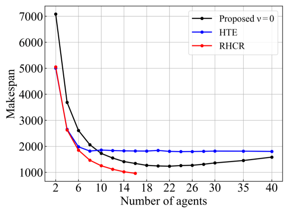
Figure 6. Makespans in Exp. 1.

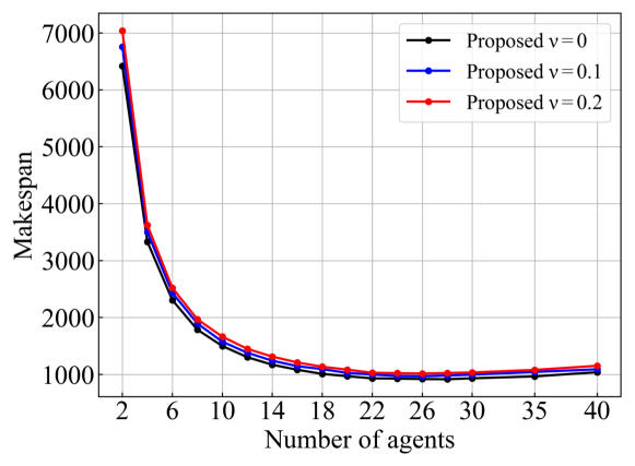
Figure 7. Makespans in Exp. 2.

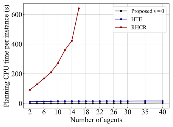
Figure 8. Planning time per instance (s) in Exp. 1.

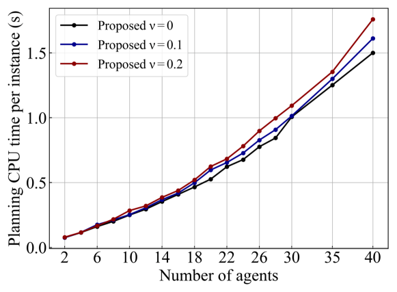
Figure 9. Planning time per instance (s) in Exp. 2.

5.2.2. Makespans

Figure 6 plots the average makespan (in timesteps) with different numbers of agents in Exp. 1. Note that the failure instances were excluded from the average calculation. This figure shows that, even if the number of agents $n$ increased to approximately six, the makespan could be shortened regardless of the methods employed.

However, when $n\geq 8$, we observed performance differences with these methods; agents with the proposed method exhibited the best performance. They could gradually decrease their makespans with an increasing number of agents up to $22$, but the performance slightly degraded when $n\geq 24$. This small degradation was caused by over-crowded areas near task endpoints by increasing the number of agents. Meanwhile, when $2\leq n\leq 6$, the performances of the baseline methods were better than that of the proposed method. Even if the number of task endpoints was not significantly large, the baseline methods enabled the agent to move the environment in parallel. However, agents with the proposed method were sometimes forced to take longer detours by following the directions of edges.

Conversely, the performance of the agents with HTE was almost constant when, $n\geq 8$. Whereas Env. 1 met the WFI conditions, it had a small number of task endpoints that were fewer than the agents. Thus, HTE could assign a limited number of tasks to agents because an agent could not select or be assigned the task whose loading or unloading node was already reserved as the task endpoints of other being executed tasks.

Although RHCR considerably outperformed other methods until $n\leq 16$ in Exp. 1, after the number exceed $16$, we could not calculate the makespan because no instances of the MAPDFS problem could be completed by RHCR owing to the congestion as discussed before. Even when $n=12$, the completion rate by agents with RHCR was $0.28$ from Table 2; it is not realistic to use RHCR in our target applications because of the low completion rate.

We plotted the average makespan for Exp. 2 in Fig. 7 to investigate the effects of the fluctuation on movement speed on the makespan in MAPDFS. This figure shows that the performance gradually decreased with increasing moving delay probability $\nu$. However, their difference is insignificant. Therefore, the result indicates that the proposed methods are robust against the fluctuation in movement speed. We also conducted the experiments by setting $T_{\it lu}=3$; however, the difference was significantly small. We believe that this effect was caused by the orientation in the main area; although an agent had to wait for loading/unloading of other agents, they started to move in the same direction according to the orientation. Thus, agents did not have to worry about head-on collisions and could wait next to where it was loading/unloading.

5.2.3. Planning (CPU) time

Figure 8 shows the averaged planning time for all agents per instance with a different number of agents in Exp. 1. We have also listed the detail of the total planning time in Table 2. Clearly, the planning time with the proposed method is much smaller than those of other methods, regardless of the number of agents. This is because, unlike HTE, agents with the proposed method could generate paths without time information and without considering other agents’ paths.

Clearly from the figure, the planning time with HTE was almost identical when the number of agents was $n\geq 10$ because the number of agents moving in parallel was limited and only the active agents generated plans. Conversely, in the proposed method, the planning time was slightly increased based on the increase in $n$, because all agents move in parallel and require time for their planning. However, even when $n=40$, the total planning time of the proposed method was only 2.78 seconds owing to the simple distributed planning. Meanwhile, RHCR required considerably large planning time (Fig. 8) because all agents are required to replan at least once in $h=15$ timesteps by interleaving planning and execution.

Figure 9 shows the averaged planning time per instance with the moving delay probability $\nu=0,0.1,0.2$ in Exp. 2. Unlike Exp.1, agents often were forced to stay longer at the same nodes in the main area due to delay by other agents and loading/unloading actions of other agents. Thus, agents might receive denial messages more frequently. However, the effect of fluctuation in movement speed on planning time was significantly small from this figure.

5.3. Discussion

The proposed method completed all tasks without collision or entering deadlock states using distributed planning with asynchronous execution in the environments that satisfy our required conditions, such as the robustness to fluctuated speed. This is because node agents prevented carrier agents from moving to the next nodes that are already reserved and/or stayed by other agents, regardless of delay owing to the speed variations, and direct edges prevented agents from crossing the same edge in opposite directions.

Furthermore, our method outperformed the baseline methods (HTE and RHCR) in environments with a small number of endpoints when the number of agents was more than 10. Our experimental results show that the proposed method can increase the concurrency of task execution and mitigate the performance degradation caused by crowded regions. HTE was unable to increase the number of concurrent task executions because the number of task endpoints was smaller than the number of agents. Further, RHCR required to replan repeatedly in all agents with synchronous planning and execution, which increased computational cost and could not complete all tasks within a reasonable time because of many live and deadlock situations caused by congestion.

In the proposed method, after an agent generated a path to the destination, it moved to the next node with local communications to check the availability and modify the path if necessary. Therefore, it was considered similar to the family of local repair algorithms with limited window size, such as traditional local repair A* Zelinsky (1992), its extension algorithms, and RHCR. A drawback of this type of algorithm is that, when many agents gather at a small number of nodes, they may cause a high likelihood of collisions, many livelock states, and many costly repairs/replanning because of congestion. However, as the proposed method introduces an orientation into the graph, it prevents, for example, an agent from being sandwiched between other agents coming from the left and right. Moreover, because agents are navigated in the direction in which they can move, even when agents’ destinations are concentrated and crowded, agents can be moved temporarily to surrounding areas to maintain their mobility.

Finally, we have to discuss more on the number of open nodes in the main area and the number of (carrier) agents. As mentioned in Section 4.5, when $|V_{\it main}|-|I|=2$, only two agents can start moving simultaneously but almost randomly. This restriction is significantly different in decentralized methods assuming synchronous movements Ma et al. (2017, 2019b); Wiktor et al. (2014); Okumura et al. (2019), in which all agents move synchronously; thus, agents can move even when $|V_{\it main}|=|I|$. However, we assumed the asynchronous movements, and such movements are impossible. Furthermore, because of the asynchrony in the distributed environments, how to move is affected by the timing of activities, such as the time/order of message arrivals. Thus, the performance is partially affected by randomness. However, in our extensive experiments using our method, agents completed all tasks.

6. Conclusion

We presented a distributed planning with asynchronous execution methods which is an efficient and robust solution for realistic environments. Our method is simple yet applicable to environments that have a smaller number of task endpoints than agents and include the fluctuated movement speed of agents. From our experiments, the proposed method outperformed baseline methods for MAPD problem and even in the environments to which they are not applicable because of variable speed and flexible endpoint locations. Our method completed all tasks efficiently without collision and deadlock in such environments.

In the future, we plan to extend our method; for example, we will relax environmental graph conditions, propose appropriate graph orienting to improve the effectiveness and efficiency, and address complex tasks (e.g., a task can be executed by multiple agents).

Appendix

Proposition 1 with Detailed Proof

We will provide the detailed proof of Proposition 1, although it is intuitively obvious.

Proposition -1.

Suppose that $G_{\it main}=G_{1}\cup\dots\cup G_{K}$ is connected graph and $G_{k}$ is the bi-connected component. If $V_{k}\cap V_{k^{\prime}}\not=\varnothing$, the $V_{k}\cap V_{k^{\prime}}$ is a singleton.

Proof.

If $V_{k}\cap V_{k^{\prime}}$ contains two nodes, $w$ and $w^{\prime}$, we can show that $V_{k}\cup V_{k^{\prime}}$ is bi-connected. Therefore, we demonstrate that, for any nodes $v\in V_{k}$ and $v^{\prime}\in V_{k^{\prime}}$, there exist two paths in $G_{k}$ between $v$ and $w$ and between $v$ and $w^{\prime}$, whose common nodes are only $v$. Thus, we can also generate two paths in $G_{k^{\prime}}$ between $v^{\prime}$ and $w$ and between $v^{\prime}$ and $w^{\prime}$, whose common nodes are only $v^{\prime}$. Then, by connecting these paths from $v$ to $v^{\prime}$ through $w$ and from $v$ to $v^{\prime}$ through $w^{\prime}$, we can proof that $V_{k}\cup V_{k^{\prime}}$ is bi-connected. First, because $G_{k}$ is bi-connected, we can generate at least two paths in $G_{k}$ connecting between $v$ and $w$ such that these paths do not have the common node, except $v$ and $w$. We denote these paths by sequences of nodes, $p_{v\shortrightarrow w}^{0}=(v_{0}^{0},v_{1}^{0},\dots,v_{h_{1}}^{0})$, and $p_{v\shortrightarrow w}^{1}=(v_{0}^{1},\dots,v_{h_{2}}^{1})$, where $v_{0}^{0}=v_{0}^{1}=v$, $v_{h_{1}}^{0}=v_{h_{2}}^{1}=w$, and $v_{l}^{0}$ and $v_{l^{\prime}}^{1}\in V_{k}$. Similarly, we can generate two paths between $v$ and $w^{\prime}$ whose common nodes are only end nodes. These paths are denoted by $p_{v\shortrightarrow w^{\prime}}^{0}=({v^{\prime}}_{0}^{0},\dots,{v^{\prime}}_{{h^{\prime}}_{1}}^{0})$ and $p_{v\shortrightarrow w^{\prime}}^{1}=({v^{\prime}}_{0}^{1},\dots,{v^{\prime}}_{{h^{\prime}}_{2}}^{1})$, where ${v^{\prime}}_{0}^{0}={v^{\prime}}_{0}^{1}=v$, ${v^{\prime}}_{h_{1}}^{0}={v^{\prime}}_{h_{2}}^{1}=w$, and ${v^{\prime}}_{l}^{0}$ and ${v^{\prime}}_{l^{\prime}}^{1}\in V_{k}$. If $\exists m\in\{0,1\}$ such that $p_{v\shortrightarrow w}^{m}$ that intersects, except at their end nodes, at most one of $p_{v\shortrightarrow w^{\prime}}^{1}$ and $p_{v\shortrightarrow w^{\prime}}^{2}$, we can select $p_{v\shortrightarrow w^{\prime}}^{m^{\prime}}$ that does not intersect $p_{v\shortrightarrow w}^{m}$. If such a path does not exist, $\forall m\in\{0,1\}$ such that $p_{v\shortrightarrow w}^{m}$ that intersects both $p_{v\shortrightarrow w^{\prime}}^{0}$ and $p_{v\shortrightarrow w^{\prime}}^{1}$. Let $v_{l}^{m}$ be the last nodes in $(v_{0}^{m},v_{1}^{m},\dots,v_{h_{m}}^{m})$ at which intersect $p_{v\shortrightarrow w^{\prime}}^{0}$ or $p_{v\shortrightarrow w^{\prime}}^{1}$. Assuming that $v_{l}^{m}$ is selected from $p_{v\shortrightarrow w^{\prime}}^{\widetilde{m}}$ (${\widetilde{m}}\in\{0,1\}$), if we consider paths $p_{v\shortrightarrow w}=({v^{\prime}}_{0}^{\widetilde{m}},\dots,{v^{\prime}}_{l^{\prime}}^{\widetilde{m}}=v_{l}^{m},\dots,v_{h}^{m},v_{h_{m}}^{m})$ and $p_{v\shortrightarrow w^{\prime}}^{1-{\widetilde{m}}}$, these have no intersection except $v$. ∎

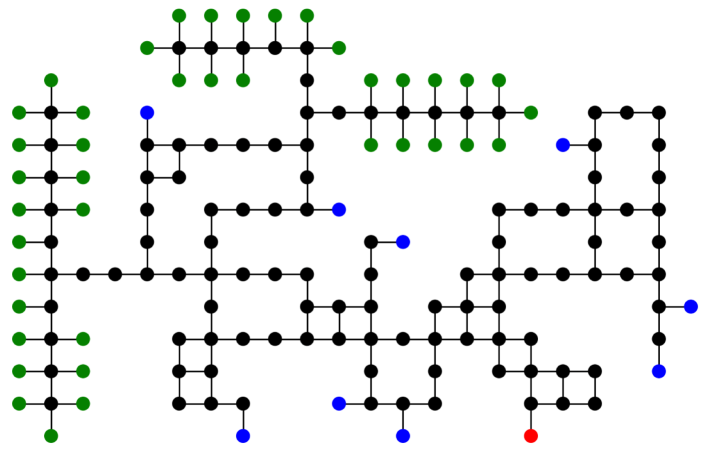
Figure 10. Example environments (Env.3).

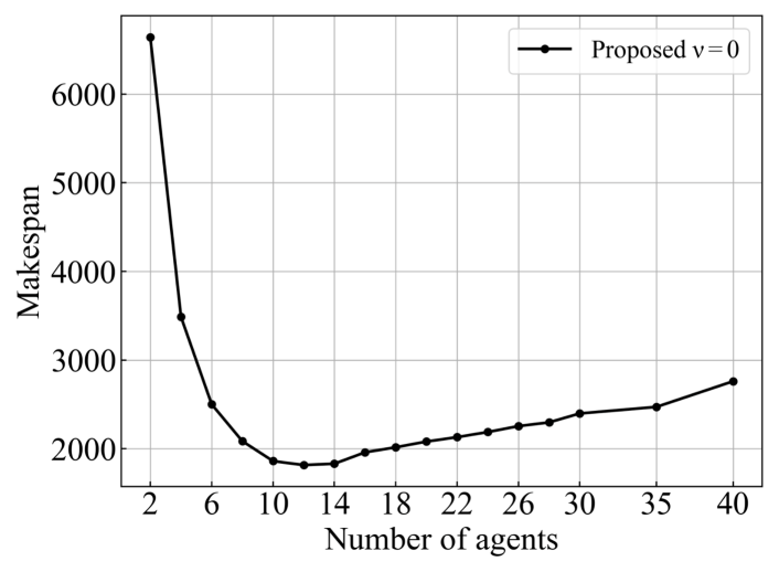
Figure 11. Makespans in Exp. 3.

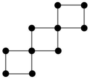
Figure 12. Example environments (Env.4).

Videos of Agents’ Movements in (Additional) Experiments

We have added videos of the agents’ movements in our experiments in this appendix. We also conducted two additional experiments to confirm whether agents using the proposed method can complete all task without collision in rare environments where over-crowded often occur. We briefly describe these experiments below.

In the first additional experiment (Exp.3), the structure of environment was identical to Exp.1, however, the loading node was selected from only red node, and the unloading nodes were selected from blue node as shown in Fig. 10. This assumes that the materials are stored at the specific place (red node) and are carried to various nodes; therefore, over-crowded situations are likely to occur around the red node.

Figure 11 plots the average makespan with different number of agents $n$ in Exp.3. Note that we conducted fifty experimental runs as in other experiments. The experimental result shows that agents using proposed method could also complete all instance in Exp.3 regardless of the number of agents whose max is $40$. The agents with proposed method could reduce the makespan along with the increasing of the number of agents to $n=12$. After that, as the number of agents increased when $n\geq 14$, the performance gradually decreased probably due to over-crowded situations around a single loading node (red node). Furthermore, we can see that makespan was considerably larger in Exp. 3 by comparing Figs. 6, 7 and 11. This is also because there is only one endpoint for loading, and thus, all agents are likely to gather this endpoint. We want to insist that agents with the proposed method still perform MAPD instances without deadlock situations as shown in the following video, indicating that our proposed methods are robust even in such a over-crowded situation.

In the second additional experiment (Exp.4), we tested the relevance between the number of nodes in main area and the number of agents, mentioned in main paper. There are eight agents running the MAPD problem instance in three bi-connected components whose the total number of nodes is ten, as shown in Fig. 12; therefore, $|V_{\it main}|-|I|=2$. We also assume that all nodes are endpoints, so an agent can be load and unload any node. All agents initially placed at the random nodes and began to perform the pickup-and-delivery tasks. We believe that this situation was pathological. However, we confirmed that agents could complete an MAPD instance in Exp.4, although agents could reach their destination almost randomly so required so long time.

The followings are list of the sample videos to show the movements of the agents using proposed method in our four experiments. Note that, due to limit of submission file size, we make the short clip of video. Note that in these videos, the direction of an edge is represented by a long triangle, whereas the undirected edge is represented by a bold line.

Experiment 1 (Exp.1)

Agents used proposed method, the number of agent was 22, the environment is Env. 1, and sample video is available at the url https://youtu.be/l4xnnsy5TJs. We can confirm that all agents were able to move around the area without collisions, although light congestion occasionally occurred in some places because several agents set the same destinations.

Experiment 2 (Exp.2)

Agents used the proposed method, the number of agent was 40, the environment is Env.2. Sample video can be found at the url https://youtu.be/do3pa22yKps. Although Env. 2 which does not meet the WFI condition and has a small negative swing, they could smoothly move around there and complete the MAPD instances.

Experiment 3 (Exp.3)

Forty agents adopting the proposed method performed the MAPD instance in the environment Env. 3. Sample video can be found at https://youtu.be/uXfgFJjgLIA. As we mentioned above, agents using proposed method could complete all instance in such a over-crowded situation.

Experiment 4 (Exp.4)

Eight agents adopting the proposed method performed the MAPD instance in the environment Env. 3 that has only ten nodes. TSample video can be found at https://youtu.be/0ap6Vq9JbBw. As we mentioned above, agents using proposed method could complete all instance when $|V_{\it main}|-|I|=2$.

References

- (1)
- Atallah (1984) Mikhail J. Atallah. 1984. Parallel strong orientation of an undirected graph. Inform. Process. Lett. 18, 1 (1984), 37–39. https://doi.org/10.1016/0020-0190(84)90072-3
- Barer et al. (2014) Max Barer, Guni Sharon, Roni Stern, and Ariel Felner. 2014. Suboptimal variants of the conflict-based search algorithm for the multi-agent pathfinding problem. In Seventh Annual Symposium on Combinatorial Search. Citeseer.
- Boyarski et al. (2015) Eli Boyarski, Ariel Felner, Roni Stern, Guni Sharon, David Tolpin, Oded Betzalel, and Eyal Shimony. 2015. ICBS: Improved Conflict-Based Search Algorithm for Multi-Agent Pathfinding. In Proceedings of the 24th Int. Conference on Artificial Intelligence (Buenos Aires, Argentina) (IJCAI’15). AAAI Press, 740–746.
- Cohen et al. (2015) Liron Cohen, Tansel Uras, and Sven Koenig. 2015. Feasibility study: Using highways for bounded-suboptimal multi-agent path finding. In Eighth Annual Symposium on Combinatorial Search. 2–8.
- Dijkstra (1976) Edsger W. Dijkstra. 1976. A Discipline of Programming. Prentice-Hall. I–XVII, 1–217 pages.
- Felner et al. (2018) Ariel Felner, Jiaoyang Li, Eli Boyarski, Hang Ma, Liron Cohen, T. K. Satish Kumar, and Sven Koenig. 2018. Adding Heuristics to Conflict-Based Search for Multi-Agent Path Finding. Proceedings of the Int. Conference on Automated Planning and Scheduling 28, 1 (Jun. 2018), 83–87.
- Huang et al. (2021) Taoan Huang, Bistra Dilkina, and Sven Koenig. 2021. Learning Node-Selection Strategies in Bounded-Suboptimal Conflict-Based Search for Multi-Agent Path Finding. In Proceedings of the 20th International Conference on Autonomous Agents and MultiAgent Systems. 611–619.
- Jennings et al. (1997) J. S. Jennings, G. Whelan, and W. F. Evans. 1997. Cooperative search and rescue with a team of mobile robots. In 1997 8th International Conference on Advanced Robotics. Proceedings. ICAR’97. 193–200.
- Li et al. (2021) Jiaoyang Li, Andrew Tinka, Scott Kiesel, Joseph W. Durham, T. K. Satish Kumar, and Sven Koenig. 2021. Lifelong Multi-Agent Path Finding in Large-Scale Warehouses. Proceedings of the AAAI Conference on Artificial Intelligence 35, 13 (May 2021), 11272–11281.
- Liu et al. (2019) Minghua Liu, Hang Ma, Jiaoyang Li, and Sven Koenig. 2019. Task and Path Planning for Multi-Agent Pickup and Delivery. In Proceedings of the 18th International Conference on Autonomous Agents and MultiAgent Systems. International Foundation for Autonomous Agents and Multiagent Systems, 1152–1160.
- Ma et al. (2019a) Hang Ma, Daniel Harabor, Peter J. Stuckey, Jiaoyang Li, and Sven Koenig. 2019a. Searching with Consistent Prioritization for Multi-Agent Path Finding. Proceedings of the AAAI Conference on Artificial Intelligence 33, 01 (Jul. 2019), 7643–7650.
- Ma et al. (2019b) Hang Ma, Wolfgang Hönig, TK Satish Kumar, Nora Ayanian, and Sven Koenig. 2019b. Lifelong path planning with kinematic constraints for multi-agent pickup and delivery. In Proceedings of the AAAI Conference on Artificial Intelligence, Vol. 33. 7651–7658.
- Ma et al. (2017) Hang Ma, Jiaoyang Li, T.K. Satish Kumar, and Sven Koenig. 2017. Lifelong Multi-Agent Path Finding for Online Pickup and Delivery Tasks. In Proceedings of the 16th Conference on Autonomous Agents and MultiAgent Systems (São Paulo, Brazil) (AAMAS ’17). International Foundation for Autonomous Agents and Multiagent Systems, Richland, SC, 837–845.
- Miyashita et al. (2022) Yuki Miyashita, Tomoki Yamauchi, and Toshiharu Sugawara. 2022. Distributed and Asynchronous Planning and Execution for Multi-agent Systems through Short-Sighted Conflict Resolution. In 2022 IEEE 46th Annual Computers, Software, and Applications Conference (COMPSAC). 14–23. https://doi.org/10.1109/COMPSAC54236.2022.00012
- Nguyen et al. (2017) Van Nguyen, Philipp Obermeier, Tran Cao Son, Torsten Schaub, and William Yeoh. 2017. Generalized Target Assignment and Path Finding Using Answer Set Programming. In Proceedings of the 26th International Joint Conference on Artificial Intelligence (Melbourne, Australia) (IJCAI’17). AAAI Press, 1216–1223.
- Okumura et al. (2019) Keisuke Okumura, Manao Machida, Xavier Défago, and Yasumasa Tamura. 2019. Priority Inheritance with Backtracking for Iterative Multi-agent Path Finding. In Proceedings of the Twenty-Eighth International Joint Conference on Artificial Intelligence (IJCAI’19). 535–542. https://doi.org/10.24963/ijcai.2019/76
- Pěchouček et al. (2006) Michal Pěchouček, David Šišlák, Dušan Pavlíček, and Miroslav Uller. 2006. Autonomous Agents for Air-Traffic Deconfliction. In Proceedings of the Fifth International Joint Conference on Autonomous Agents and Multiagent Systems (Hakodate, Japan) (AAMAS ’06). Association for Computing Machinery, New York, NY, USA, 1498–1505. https://doi.org/10.1145/1160633.1160925
- Robbins (1939) Herbert E. Robbins. 1939. A Theorem on Graphs, with an Application to a Problem of Traffic Control. Amer. Math. Monthly 46 (1939), 281.
- Salzman and Stern (2020) Oren Salzman and Roni Stern. 2020. Research Challenges and Opportunities in Multi-Agent Path Finding and Multi-Agent Pickup and Delivery Problems. In Proceedings of the 19th International Conference on Autonomous Agents and MultiAgent Systems. 1711–1715.
- Sharon et al. (2015) Guni Sharon, Roni Stern, Ariel Felner, and Nathan R Sturtevant. 2015. Conflict-based search for optimal multi-agent pathfinding. Artificial Intelligence 219 (2015), 40–66.
- Švancara et al. (2019) Jiří Švancara, Marek Vlk, Roni Stern, Dor Atzmon, and Roman Barták. 2019. Online multi-agent pathfinding. In Proceedings of the AAAI Conference on Artificial Intelligence, Vol. 33. 7732–7739.
- Tarjan (1972) Robert Tarjan. 1972. Depth-First Search and Linear Graph Algorithms. SIAM J. Comput. 1, 2 (1972), 146–160. https://doi.org/10.1137/0201010
- Čáp et al. (2015) Michal Čáp, Jiří Vokřínek, and Alexander Kleiner. 2015. Complete Decentralized Method for On-Line Multi-Robot Trajectory Planning in Well-Formed Infrastructures. In Proceedings of the Twenty-Fifth International Conference on International Conference on Automated Planning and Scheduling (Jerusalem, Israel) (ICAPS’15). AAAI Press, 324–332.
- Wan et al. (2018) Qian Wan, Chonglin Gu, Sankui Sun, Mengxia Chen, Hejiao Huang, and Xiaohua Jia. 2018. Lifelong Multi-Agent Path Finding in A Dynamic Environment. In 2018 15th International Conference on Control, Automation, Robotics and Vision (ICARCV). 875–882. https://doi.org/10.1109/ICARCV.2018.8581181
- Wiktor et al. (2014) A. Wiktor, D. Scobee, S. Messenger, and C. Clark. 2014. Decentralized and complete multi-robot motion planning in confined spaces. In 2014 IEEE/RSJ International Conference on Intelligent Robots and Systems. 1168–1175.
- Wilt and Botea (2014) Christopher Wilt and Adi Botea. 2014. Spatially Distributed Multiagent Path Planning. In Proceedings of the Twenty-Fourth International Conferenc on International Conference on Automated Planning and Scheduling (Portsmouth, New Hampshire, USA) (ICAPS’14). AAAI Press, 332–340.
- Yamauchi et al. (2022) Tomoki Yamauchi, Yuki Miyashita, and Toshiharu Sugawara. 2022. Standby-Based Deadlock Avoidance Method for Multi-Agent Pickup and Delivery Tasks. In Proceedings of the 21st International Conference on Autonomous Agents and Multiagent Systems (Virtual Event, New Zealand) (AAMAS ’22). International Foundation for Autonomous Agents and Multiagent Systems, Richland, SC, 1427–1435.
- Yan et al. (2013) Zhi Yan, Nicolas Jouandeau, and Arab Ali Cherif. 2013. A Survey and Analysis of Multi-Robot Coordination. International Journal of Advanced Robotic Systems 10, 12 (2013), 399. https://doi.org/10.5772/57313 arXiv:https://doi.org/10.5772/57313
- Yu and LaValle (2013) Jingjin Yu and Steven M. LaValle. 2013. Structure and Intractability of Optimal Multi-Robot Path Planning on Graphs. In Proceedings of the Twenty-Seventh AAAI Conference on Artificial Intelligence (Bellevue, Washington) (AAAI’13). AAAI Press, 1443–1449.
- Zelinsky (1992) A. Zelinsky. 1992. A mobile robot exploration algorithm. IEEE Transactions on Robotics and Automation 8, 6 (1992), 707–717. https://doi.org/10.1109/70.182671