A Federated Approach for Hate Speech Detection

Abstract

Hate speech detection has been the subject of high research attention, due to the scale of content created on social media. In spite of the attention and the sensitive nature of the task, privacy preservation in hate speech detection has remained under-studied. The majority of research has focused on centralised machine learning infrastructures which risk leaking data. In this paper, we show that using federated machine learning can help address privacy the concerns that are inherent to hate speech detection while obtaining up to $6.81\%$ improvement in terms of F1-score.

1 Introduction

Content moderation is a topic that intersects across multiple fundamental rights, e.g., freedom of expression and the right to privacy; and interest groups, e.g. scholars, legislators, civil society, and commercial entities Kaye (2019). The availability of public datasets has been crucial to the development of computational methods for hate speech detection. However, public data contains risks for those whose content is available. On the other hand, privately held data, e.g., data held by corporate entities, holds risks for those who are reporting content. Such risks may be actualised through information leaks in models Hitaj et al. (2017) or the transmission of data Shokri and Shmatikov (2015), and can impact people’s safety and livelihood.

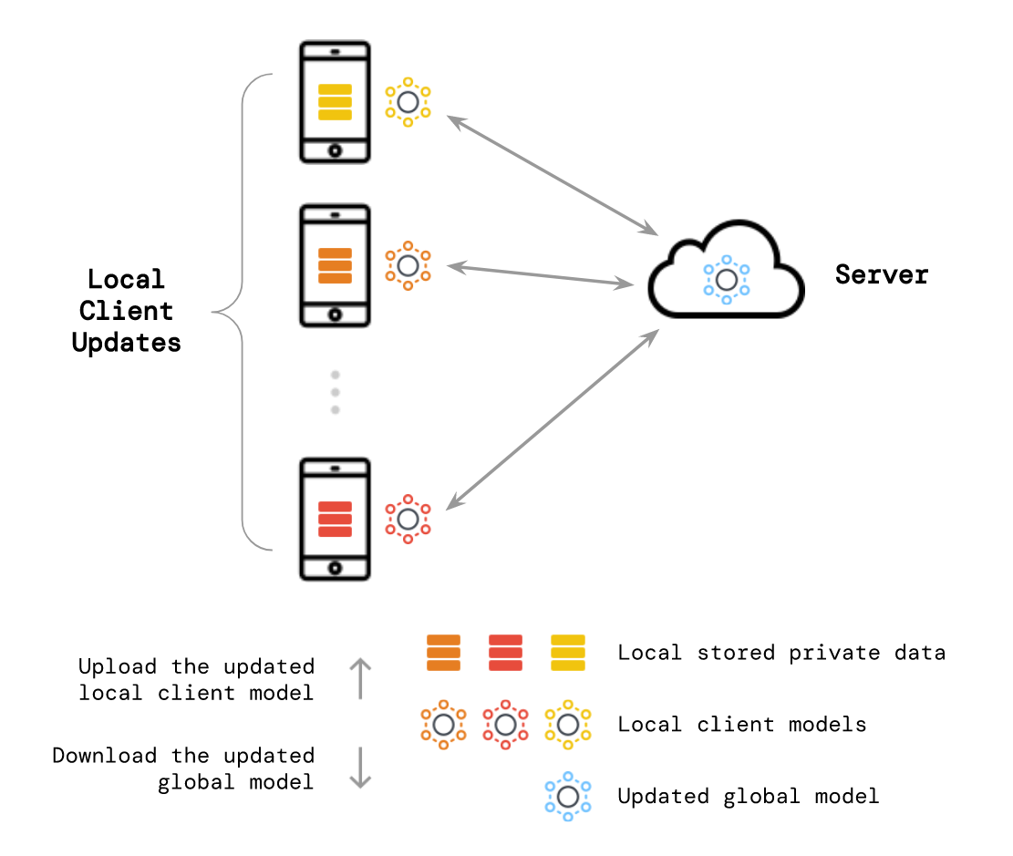
Figure 1: Federated Learning: A centralised model is hosted on a server and is distributed to client devices, these compute weight updates, and transmit the updates for aggregation into the centralised model. The centralised model is then redistributed to client devices.

In this work, we apply Federated Learning (FL, McMahan et al., 2017) to address the lack of privacy in hate speech detection. FL is a privacy-preserving training paradigm for machine learning that jointly optimises for user privacy and model performance. We posit that privacy is necessary for users whose content is flagged and users who are flagging content alike. We thus operationalise privacy, in the context of hate speech detection and federated learning, to mean privacy in terms of the content of reported content, and the report itself. FL is an apt training paradigm for tasks in which training data is highly sensitive, as FL is designed to mitigate risks of information leaks while also dealing with a high number of end-users, information loss, and label imbalances Lin et al. (2022); Priyanshu and Naidu (2021); Gandhi et al. (2022). We apply the FL algorithms FedProx (Li et al., 2020) and Adaptive Federated Optimization (FedOpt, Reddi et al., 2021) to $5$ machine learning algorithms. We evaluate our approach on $8$ previously published datasets for hate speech detection. While using FL often implies a trade-off between privacy and performance, we obtain performance improvements of up to $6.81\%$ in F1-score. We find that that models trained using FL outperform centralised models across multiple tests (e.g., derogatory language, spelling variation, and pronoun reference) in HateCheck Röttger et al. (2021).

2 Prior Work

Although the areas of hate speech detection and FL have each been subject to extensive research, the study of their intersection remains in its infancy.

Federated Learning

Federated Learning is a privacy-preserving machine learning paradigm that aims to reduce privacy risks by decentralising data processing onto client devices (i.e., personal devices), thereby foregoing the need for transmitting “raw” user data, and thus minimising risks of personal data leaks caused by transmission of data. In FL, the machine learning model is located in two places: On a centralised server, and on client devices, which hold instances of the model distributed from the centralised model.Client devices use the model to compute model updates. The model updates are then transmitted to the server and aggregated by the centralised model, which is redistributed to the client devices. However, not all transmitted weight updates are aggregated into the model. FL operates with a notion of data loss in its design, which is emulated by selecting a fraction of clients whose updates are aggregated. Thus, FL paradigm uses less data to train a models.

In our experiments, we apply two FL algorithms: FedProx and FedOpt Reddi et al. (2021). FedProx introduces a proximal term to the Federated Averaging algorithm (FedAvg, McMahan et al., 2017). FedAvg averages the weights computed on participating client devices in a round. FedProx introduces a proximal term that functions as a regulariser to the weight updates transmitted by participating clients, which penalises local weight updates that diverge from the global model. The FedAvg algorithm can thus be understood as a special case of FedProx with the proximal term set to $0.0$.

FedOpt (Reddi et al., 2021) extends the adaptive optimisation strategies from centralised optimisation (e.g., Adam Kingma and Ba (2015) and Adagrad Duchi et al. (2010)) to explicitly account for client and server optimisation. FedOpt handles server optimisation distinctly from client optimisation, by introducing a state to the server-side optimisation routine. . This distinct handling of server-side optimization enables more accurate and heterogeneity-aware FL models, which can speed up convergence.

FL has been applied to a number of tasks, including emoji prediction Ramaswamy et al. (2019); Gandhi et al. (2022), next-word prediction for mobile keyboards Yang et al. (2018), pre-training and fine-tuning large language models Liu and Miller (2020), medical named entity recognition Ge et al. (2020), and text classification Lin et al. (2022). For instance, Lin et al. (2022) used FL to fine-tune a DistilBERT model to perform classification on the 20NewsGroup dataset Lang (1995) using three different FL algorithms: FedAvg (McMahan et al., 2017), FedProx (Li et al., 2020), FedOpt (Reddi et al., 2021)) under non-IID partitioning.

In a closely related study, Basu et al. (2021) apply FL, using the FedAvg algorithm to fine-tune large language models to detect depression and sexual harassment from small Twitter data samples. They find that using large language models such as BERT and RoBERTa outperform distilled language models such as DistilBERT. Our work extends on Basu et al. (2021) by introducing additional FL algorithms and extending to a multi-class setting for hate speech detection.

Thus, our work extends on prior work by i) applying FL to the task of multi-class hate speech detection, a task which has proven difficult in part due to the complex nature of pragmatics Röttger et al. (2021) and hate mongers seeking to evade content moderation infrastructures Crawford and Gillespie (2016); ii) using the FedProx and FedOpt algorithms rather than the FedAvg algorithm, thereby reducing model vulnerability to divergent weight updates; and iii) providing an in-depth analysis of federated model performances.

Hate Speech Detection

Prior work on hate speech detection has primarily focused on privacy-agnostic machine learning paradigms, using centralised models for classification. Such work has investigated a number of machine learning models (e.g. SVMs Karan and Šnajder (2018), CNNs Park and Fung (2017), and fine-tuned language models (Swamy et al., 2019b)) and the development of resources (e.g. Talat and Hovy, 2016). Recently, Fortuna et al. (2021) proposed a standardisation of classes across $9$ publicly available datasets and studied the generalisation capabilities of BERT, fastText, and SVM models. In their work they found limited success in inter-dataset generalization. Our work thus extends on the task of hate speech detection by introducing privacy-preserving methods to multi-class hate speech detection. In doing so, the privacy of those who flag content and those whose content is flagged remain intact.

Category	Merged count	Comb	Change
aggression	$6,950$	$6,950$	-
aggressive hate speech	$1,561$	$1,561$	-
covert aggression	$4,242$	$4,242$	-
hate speech	$13,222$	$13,205$	$-0.13\%$
insult	$7,879$	$7,779$	$-1.27\%$
misogyny sexism	$5,000$	$5,000$	-
none	$189,869$	$188,550$	$-0.69\%$
offensive	$19,192$	$19,192$	-
overt aggression	$2,710$	$2,710$	-
racism	$1,978$	$1,978$	-
severely toxic	$1,597$	$1,527$	$-4.38\%$
threat	$480$	$470$	$-2.08\%$
toxicity	$40,316$	$40,134$	$-0.45\%$

Table 1: Label count of the raw datasets and Comb

		Logistic Regression			Bi-LSTM			FNet			DistilBERT			RoBERTa
		Precision	Recall	F1	Precision	Recall	F1	Precision	Recall	F1	Precision	Recall	F1	Precision	Recall	F1
c = $10\%$	e = 1	$70.22$	$53.15$	$58.47$	$71.04$	$58.19$	$61.28$	$72.61$	$59.20$	$62.20$	$73.98$	$60.75$	$63.79$	$74.76$	$64.43$	$66.16$
	e = 5	$70.83$	$63.31$	$66.35$	$70.84$	$66.51$	$67.72$	$73.52$	$68.33$	70.42	$74.54$	$69.46$	$70.85$	$74.59$	$69.68$	$71.48$
	e = 20	$70.18$	$67.41$	$68.67$	$69.17$	$69.25$	$69.10$	$73.10$	$68.02$	$69.73$	$73.28$	$71.06$	$71.94$	$73.11$	71.48	72.07
c = 30%	e = 1	71.23	$53.50$	$58.89$	$71.58$	$58.82$	$61.72$	$73.62$	$61.13$	$63.97$	$74.84$	$64.03$	$66.14$	$75.02$	$64.33$	$66.41$
	e = 5	$70.82$	$64.44$	$67.01$	$70.65$	$65.90$	$67.27$	$73.35$	$68.30$	$70.36$	$74.82$	$69.44$	$70.68$	$74.41$	$69.98$	$71.81$
	e = 20	$70.30$	68.13	69.09	$69.34$	69.26	69.15	$72.35$	$68.03$	$69.74$	$73.33$	$71.39$	$72.15$	$73.65$	$70.86$	$71.96$
c = 50%	e = 1	$71.11$	$53.12$	$58.58$	71.59	$58.71$	$61.73$	73.93	$61.89$	$64.51$	74.88	$63.58$	$65.85$	$74.42$	$63.57$	$65.87$
	e = 5	$70.89$	$64.26$	$66.80$	$70.70$	$66.16$	$67.54$	$72.90$	$68.27$	$70.18$	$74.44$	$69.68$	$70.88$	74.90	$69.46$	$70.86$
	e = 20	$70.28$	$68.00$	$69.01$	$69.25$	$68.84$	$68.20$	$72.90$	68.42	$70.16$	$73.71$	71.51	72.34	$73.53$	$71.18$	$72.01$

Table 2: Results of FedProx experiments on Comb.

		Logistic Regression			Bi-LSTM			FNet			DistilBERT			RoBERTa
		Precision	Recall	F1	Precision	Recall	F1	Precision	Recall	F1	Precision	Recall	F1	Precision	Recall	F1
c = 10%	e = 1	$68.29$	$52.48$	$58.46$	71.80	$58.34$	$61.70$	$72.64$	$59.78$	$62.49$	$74.51$	$63.87$	$65.03$	$72.02$	$64.21$	$64.57$
	e = 5	$68.20$	$59.38$	$63.14$	$70.63$	$63.73$	$66.10$	$72.39$	$69.11$	$70.51$	$74.33$	$69.61$	$70.48$	75.55	$69.44$	$70.34$
	e = 20	68.30	$59.56$	$63.23$	$69.74$	$65.32$	$67.27$	$71.87$	70.69	71.15	$72.21$	71.34	71.66	$73.17$	72.20	72.61
c = 30%	e = 1	$67.68$	$51.05$	$57.19$	$71.56$	$58.97$	$62.10$	$72.24$	$57.11$	$61.21$	74.90	$64.16$	$66.79$	$73.88$	$66.07$	$65.79$
	e = 5	$66.65$	$60.31$	$63.10$	$69.48$	$62.63$	$65.57$	$72.01$	$69.14$	$70.30$	$72.82$	$69.59$	$70.75$	$74.38$	$71.54$	$71.69$
	e = 20	$67.18$	$62.50$	64.60	$69.74$	$65.69$	$67.49$	$71.91$	$70.02$	$70.79$	$71.55$	$70.33$	$70.86$	$72.97$	$72.10$	$72.05$
c = 50%	e = 1	$67.25$	$54.85$	$59.82$	$71.35$	$59.63$	$62.59$	73.03	$62.28$	$64.64$	$73.31$	$63.98$	$65.64$	$74.85$	$66.80$	$67.75$
	e = 5	$66.63$	$60.21$	$63.04$	$69.56$	$63.02$	$65.58$	$70.63$	$68.06$	$69.21$	$72.53$	$69.66$	$70.80$	$73.78$	$71.27$	$71.18$
	e = 20	$66.70$	62.51	$64.41$	$69.16$	66.16	67.54	$70.98$	$69.74$	$70.21$	$70.65$	$68.99$	$69.69$	$72.67$	$70.51$	$71.51$

Table 3: Results of FedOpt experiments on Comb.

	Centralised			Federated
	Precision	Recall	F1	F1
LogReg	$69.11$	$57.45$	$62.20$	$69.09$
Bi-LSTM	$71.43$	$66.64$	$67.90$	$69.15$
FNet	$71.35$	$64.73$	$66.58$	$71.15$
DistilBERT	$73.99$	$69.01$	$69.39$	$72.34$
RoBERTa	$\mathbf{75.45}$	$\mathbf{70.58}$	$\mathbf{71.03}$	$\mathbf{72.61}$

Table 4: Results for the centralised and best performing FL models. The FL models have been chosen across FedProx and FedOpt based on F1 scores.

3 Data

We combine our dataset using the standardisation schema proposed by Fortuna et al. (2021).

Comb

We reuse $8$ of the $9$ datasets used by Fortuna et al. (2021) to form Comb. Comb then consists of the datasets proposed by Talat and Hovy (2016); Davidson et al. (2017); Fersini et al. (2018); de Gibert et al. (2018); Swamy et al. (2019b); Basile et al. (2019); Zampieri et al. (2019) and the Kaggle toxic comment challenge. We perform a stratified split of all training data into training (70%), validation (10%), and test (20%) sets.

Data Cleaning

We address issues of extreme class imbalance in Comb by removing the “abusive” category as it only contains $2$ documents. Following an in-depth analysis of the Kaggle dataset we find that the maximum length of tokens in the dataset is $4950$ while the median length of tokens in Comb is $26$. Moreover, we find that the longest $1\%$ of documents in the Kaggle dataset do not contain unique tokens. Removing the longest $1\%$ of comments reduces the maximal document length to $727$ tokens (see Section B.3 for further detail). Following our data cleaning processes, Comb comes to consist of $293,300$ documents (see Table 1 for an overview of changes).

4 Experiments

We experiment with $5$ machine learning models in their centralised and federated settings: Logistic Regression Bi-LSTMs (Hochreiter and Schmidhuber, 1997), FNet (Lee-Thorp et al., 2022), DistilBERT (Sanh et al., 2019) and RoBERTa (Liu et al., 2019). We measure their performance using weighted F1 scores. The centralised models form our baselines, while the federated models form our experimental models. For the Logistic Regression and Bi-LSTMs, we perform word-level tokenisation using SpaCy (Honnibal and Montani, 2017). For the FNet, DistilBERT, and RoBERTa, we use the tokenisers provided with each model.

4.1 Federated Training

FL is a machine learning training paradigm that distributes training onto client devices. All client devices are split into overlapping subsets and the training data is partitioned and uniformly distributed to client devices. A random client subset is selected for training in each round, and their locally computed weights are aggregated on the server. We train our models for $300$ rounds for $1$, $5$, or $20$ epochs per round, and set the client fraction to $10\%$, $30\%$, or $50\%$ which are randomly sampled from $100$ client devices. We perform hyper-parameter tuning for the client learning rate, server-side learning rate, and proximal term (see section B.1).

In our work, we conceptualise client devices as users who witness and report hate speech. We simulate the client devices and ensure that data is independently and identically distributed (I.I.D.) on client devices. We use the FedProx and FedOpt algorithms to aggregate client updates on the server. FedProx introduces a regularisation constant to the server-side aggregation step, the proximal term to address issues of divergence in weights and statistical heterogeneity in FedAvg. FedOpt seeks to create more robust models by introducing a separate optimiser for the server-side model to account for data heterogeneity.

5 Analysis

Considering the baseline models in Table 4, we see that the Logistic Regression tends to under-perform, while the RoBERTa model posts the best performances. Although FL-based models often outperform our baselines, we note that when FL models are trained with lower client fractions and epochs, they tend to be outperformed by the baselines. Models trained using FedProx outperform the centralised baselines (see table 2). For instance, we see large improvements for FNet and Logistic Regression ($4.5$ and $6.8$ points in terms of F1- score, respectively). Comparing the performances of models trained using FedOpt (table 3) with those trained using FedProx, we observe that the former (in particular FNet and RoBERTa) tend to outperform the latter for lower client fractions and epochs. In general, we find that the best FL models outperform their centralised counter-parts (see Tables 2 and 3). In fact, the best performing RoBERTa, DistilBERT, and FNet models trained using FL algorithms outperform their centralised baselines, with FNet obtaining a $3$-$4$ point improvement over centralised models in terms of F1 score.

While FL often indicates a trade-off between privacy and performance, we find that the best FL models outperform the centralised baselines. We believe that the improved performance stems from the dataset being split into smaller segments, in congruence with findings from prior work. For instance, Nobata et al. (2016) show that splitting data into smaller temporal segments helped improve classification performance overall. We believe that a similar effect may be evident with FL models that, by design split data into small segments and disregard a fraction of the clients. Further, it may be the case that some data within hate speech datasets hinders generalisation. Only using subsets of the data for training may therefore aid generalisation.

5.1 Hate Check Evaluation

Functionality	Accuracy (%)
	Logistic Regression			Bi-LSTM			FNet			DistilBERT			RoBERTa
	Central	Fprox	FOpt	Central	Fprox	FOpt	Central	Fprox	FOpt	Central	Fprox	FOpt	Central	Fprox	FOpt
F1: Expression of strong negative emotions (explicit)	$96.4$	$\mathbf{100.0}$	$97.1$	$80.7$	$\mathbf{100.0}$	$95.7$	$75.0$	$\mathbf{98.6}$	$97.9$	$90.0$	$\mathbf{99.3}$	$87.9$	$89.3$	$87.9$	$\mathbf{92.9}$
F2: Description using very negative attributes (explicit)	$95.0$	$\mathbf{100.0}$	$97.9$	$65.7$	$99.3$	$99.3$	$87.1$	$\mathbf{100.0}$	$\mathbf{100.0}$	$96.4$	$\mathbf{100.0}$	$97.7$	$92.9$	$93.6$	$\mathbf{95.0}$
F3: Dehumanisation (explicit)	$97.9$	$\mathbf{100.0}$	$94.3$	$77.9$	$\mathbf{100.0}$	$\mathbf{100.0}$	$85.0$	$\mathbf{100.0}$	$\mathbf{100.0}$	$97.1$	$\mathbf{100.0}$	$93.6$	$90.7$	$\mathbf{94.3}$	$\mathbf{94.3}$
F4: Implicit derogation	$87.1$	$\mathbf{95.7}$	$75.7$	$70.7$	$\mathbf{94.3}$	$92.9$	$62.1$	$\mathbf{99.3}$	$96.4$	$72.9$	$\mathbf{82.9}$	$\mathbf{82.9}$	$77.1$	$78.6$	$\mathbf{80.7}$
F5: Direct threat	$90.2$	$\mathbf{99.3}$	$94.0$	$80.0$	$\mathbf{96.2}$	$88.0$	$82.0$	$\mathbf{100.0}$	$98.5$	$88.0$	$\mathbf{98.5}$	$91.7$	$91.0$	$\mathbf{95.5}$	$91.7$
F6: Threat as normative statement	$94.3$	$\mathbf{99.3}$	$96.4$	$80.7$	$\mathbf{99.3}$	$98.6$	$70.0$	$\mathbf{100.0}$	$\mathbf{100.0}$	$90.0$	$\mathbf{100.0}$	$94.3$	$\mathbf{96.4}$	$90.7$	$91.4$
F7: Hate expressed using slur	$87.5$	$\mathbf{99.3}$	$98.6$	$75.7$	$88.2$	$\mathbf{96.5}$	$86.1$	$\mathbf{98.6}$	$96.5$	$91.0$	$\mathbf{94.4}$	$90.0$	$\mathbf{88.2}$	$84.7$	$86.1$
F8: Non-hateful homonyms of slurs	$6.7$	$16.7$	$\mathbf{43.3}$	$10.0$	$\mathbf{43.3}$	$40.0$	$16.7$	$23.3$	$\mathbf{26.7}$	$23.3$	$\mathbf{50.0}$	$33.3$	$26.7$	$\mathbf{40.0}$	$36.7$
F9: Reclaimed slurs	$4.9$	$4.9$	$\mathbf{40.7}$	$2.5$	$\mathbf{42.0}$	$27.2$	$9.9$	$11.1$	$\mathbf{13.6}$	$6.2$	$7.4$	$\mathbf{12.4}$	$4.9$	$16.1$	$\mathbf{17.3}$
F10: Hate expressed using profanity	$\mathbf{100.0}$	$\mathbf{100.0}$	$\mathbf{100.0}$	$93.6$	$\mathbf{96.4}$	$\mathbf{96.4}$	$94.3$	$\mathbf{100.0}$	$\mathbf{100.0}$	$97.9$	$\mathbf{100.0}$	$\mathbf{100.0}$	$\mathbf{100.0}$	$\mathbf{100.0}$	$\mathbf{100.0}$
F11: Non-hateful use of profanity	$2.0$	$13.0$	$\mathbf{38.0}$	$19.0$	$\mathbf{47.0}$	$40.0$	$6.0$	$11.0$	$\mathbf{19.0}$	$15.0$	$13.0$	$\mathbf{16.0}$	$3.0$	$11.0$	$\mathbf{17.0}$
F12: Hate expressed through reference in subsequent clauses	$\mathbf{100.0}$	$\mathbf{100.0}$	$90.0$	$91.4$	$\mathbf{98.6}$	$\mathbf{98.6}$	$86.4$	$\mathbf{100.0}$	$\mathbf{100.0}$	$95.0$	$\mathbf{98.6}$	$96.4$	$90.0$	$\mathbf{92.9}$	$92.1$
F13: Hate expressed through reference in subsequent sentences	$\mathbf{100.0}$	$\mathbf{100.0}$	$96.2$	$85.0$	$\mathbf{96.2}$	$94.7$	$84.2$	$\mathbf{100.0}$	$\mathbf{100.0}$	$95.5$	$\mathbf{99.3}$	$97.0$	$\mathbf{96.2}$	$94.0$	$95.5$
F14: Hate expressed using negated positive statement	$92.9$	$\mathbf{99.3}$	$84.3$	$57.9$	$89.3$	$\mathbf{93.6}$	$52.1$	$\mathbf{100.0}$	$\mathbf{100.0}$	$77.9$	$\mathbf{93.6}$	$76.4$	$61.4$	$81.4$	$\mathbf{90.7}$
F15: Non-hate expressed using negated hateful statement	$6.0$	$30.0$	$\mathbf{58.7}$	$25.6$	$\mathbf{53.4}$	$41.4$	$27.1$	$23.3$	$\mathbf{33.8}$	$17.3$	$27.1$	$\mathbf{43.6}$	$31.6$	$51.1$	$\mathbf{56.4}$
F16: Hate phrased as a question	$95.7$	$\mathbf{100.0}$	$95.0$	$81.4$	$93.6$	$\mathbf{96.4}$	$61.4$	$\mathbf{95.0}$	$\mathbf{95.0}$	$92.1$	$\mathbf{96.4}$	$91.4$	$82.1$	$\mathbf{95.0}$	$87.9$
F17: Hate phrased as an opinion	$99.0$	$\mathbf{100.0}$	$92.5$	$89.5$	$\mathbf{99.0}$	$97.7$	$81.2$	$\mathbf{100.0}$	$94.0$	$91.0$	$\mathbf{98.5}$	$93.2$	$86.5$	$\mathbf{93.2}$	$87.2$
F18: Neutral statements using protected group identifiers	$20.6$	$56.3$	$\mathbf{77.0}$	$42.1$	$\mathbf{75.4}$	$62.7$	$50.0$	$55.6$	$\mathbf{69.0}$	$69.0$	$68.3$	$\mathbf{75.4}$	$69.0$	$\mathbf{92.9}$	$87.3$
F19: Positive statements using protected group identifiers	$18.0$	$42.9$	$\mathbf{80.0}$	$46.0$	$\mathbf{64.6}$	$41.3$	$45.5$	$37.0$	$\mathbf{59.3}$	$38.6$	$49.2$	$\mathbf{73.1}$	$48.1$	$78.8$	$\mathbf{92.1}$
F20: Denouncements of hate that quote it	$1.7$	$19.0$	$\mathbf{55.5}$	$14.5$	$\mathbf{44.5}$	$28.3$	$31.2$	$\mathbf{45.1}$	$33.5$	$16.2$	$\mathbf{48.6}$	$38.7$	$15.6$	$36.4$	$\mathbf{37.0}$
F21: Denouncements of hate that make direct reference to it	$4.2$	$15.6$	$\mathbf{47.5}$	$21.3$	$\mathbf{46.8}$	$36.9$	$27.7$	$22.7$	$\mathbf{34.0}$	$12.1$	$16.3$	$\mathbf{30.5}$	$19.1$	$39.0$	$\mathbf{43.3}$
F22: Abuse targeted at objects	$10.8$	$45.1$	$\mathbf{70.8}$	$46.1$	$\mathbf{70.8}$	$52.3$	$53.8$	$47.7$	$\mathbf{58.5}$	$55.4$	$\mathbf{66.2}$	$\mathbf{66.2}$	$60.0$	$73.8$	$\mathbf{75.4}$
F23: Abuse targeted at individuals (not as member of a prot. group)	$4.6$	$29.2$	$\mathbf{61.5}$	$29.2$	$\mathbf{69.2}$	$52.3$	$20.0$	$24.6$	$\mathbf{38.5}$	$20.0$	$29.2$	$\mathbf{38.5}$	$23.1$	$15.4$	$\mathbf{69.2}$
F24: Abuse targeted at non-protected groups (e.g. professions)	$14.5$	$24.2$	$\mathbf{62.9}$	$27.4$	$\mathbf{74.2}$	$53.2$	$35.5$	$40.3$	$\mathbf{46.8}$	$41.9$	$43.5$	$\mathbf{59.7}$	$29.0$	$45.2$	$\mathbf{66.1}$
F25: Swaps of adjacent characters	$97.7$	$\mathbf{99.2}$	$90.2$	$82.7$	$\mathbf{95.5}$	$\mathbf{95.5}$	$72.2$	$\mathbf{98.5}$	$\mathbf{98.5}$	$78.2$	$\mathbf{97.0}$	$78.9$	$71.4$	$\mathbf{89.5}$	$80.5$
F26: Missing characters	$83.8$	$\mathbf{100.0}$	$81.6$	$72.8$	$97.1$	$\mathbf{98.8}$	$74.6$	$\mathbf{97.7}$	$92.4$	$84.4$	$94.8$	$\mathbf{98.8}$	$89.0$	$90.2$	$\mathbf{92.5}$
F27: Missing word boundaries	$97.9$	$\mathbf{100.0}$	$99.2$	$82.3$	$\mathbf{100.0}$	$\mathbf{100.0}$	$79.4$	$\mathbf{100.0}$	$93.6$	$79.4$	$\mathbf{90.8}$	$86.5$	$\mathbf{93.6}$	$90.8$	$90.8$
F28: Added spaces between chars	$83.8$	$\mathbf{100.0}$	$86.1$	$72.8$	$97.1$	$\mathbf{98.8}$	$74.6$	$\mathbf{97.7}$	$92.5$	$84.4$	$94.8$	$\mathbf{98.8}$	$89.0$	$90.1$	$\mathbf{92.5}$
F29: Leet speak spellings	$99.4$	$\mathbf{100.0}$	$98.8$	$80.9$	$\mathbf{99.4}$	$98.8$	$65.9$	$\mathbf{98.2}$	$93.6$	$75.1$	$\mathbf{84.4}$	$75.1$	$75.1$	$83.8$	$\mathbf{86.7}$

Table 5: Results on the HateCheck test suite.

This section extends the experiments to qualitatively evaluate the effectiveness of federated and centralised models under different axis of hate speech using HateCheck Röttger et al. (2021). HateCheck is a suite of functional tests for hate speech detection models. HateCheck provides an in-depth examination of model performances across different potential challenges for machine learning models trained for hate speech detection.

The HateCheck Röttger et al. (2021) dataset consists of $29$ tests, $18$ of which test for distinct expressions of hate while the remaining $11$ test for non-hateful expressions. The dataset contains $3.728$ labelled samples, $69\%$ of which are ‘Hate‘ and while the remaining $31\%$ are labelled as ‘Not-Hate‘. We evaluate all the models that have been trained for this manuscript, including the model examined in appendix A. We evaluate our trained models HateCheck’s binary form by mapping all classes positive classes to “hate” and the negative class to “not-hate”.

Conducting the HateCheck functional tests for the models trained on the Comb dataset, we see (please refer to table 5) that the federated learning models perform on par or better than the centralised models on a macro scale. The federated Bi-LSTM and FNet models yield strong improvement of 3 - 5%. On the other hand, there is a slight performance dip (0.5 - 1%) for the federated DistilBERT and RoBERTa models. Moreover, through a fine-grained analysis of model performance, we observe that all the models (centralised and federated) perform acceptable performances for different types of derogatory, pronoun reference, phrasing, spelling variations, and threatening language. However, all models perform poorly for the tests for counter speech, indicating that while the models learn to recognise some forms of hate, they cannot accurately recognise responses to it. Furthermore, we see that RoBERTa performs slightly better than all the other model variants on non-hate group identity and abuse against non-protected targets. RoBERTa and DistilBERT achieve the best performances for slurs. Overall, we find that RoBERTa and DistilBERT consistently perform well across many of the functional tests which might be due to having been pre-trained on large amount of language data. However, the pre-training also induces certain biases which limit the models’ performance on profanity. The Bi-LSTMs outperform all the models on non-hateful profanity but simultaneously under-perform on hateful profanity.

6 Conclusion

Private and sensitive data can risk being exposed when developing and deploying models for hate speech detection. We therefore examine the use of Federated Learning, a privacy preserving machine learning paradigm to the task of hate speech detection to emphasise privacy in hate speech detection. We find that using Federated Learning improves on the performance levels achieved using centralised models, thus affording both privacy and performance. In future work, we intend to examine interpretability and explainability for federated learning to gain a better understanding of the causes of such performance increases.

Limitations

While Federated Learning introduces increased privacy in the process of hate speech detection, a real time system may be vulnerable to attacks that can lead to privacy leakages. For instance, the weights being transferred from the clients to the server may reveal information about the local dataset to an adversary (Bhowmick et al., 2018; Melis et al., 2019). However unintended these leakages may be, they still pose a significant threat and might limit the privacy claim.

The Federated Learning models trained in our work rely on $8$ of the $9$ datasets used by Fortuna et al. (2021), as we could not gain access to the final dataset. We do not test the biases introduced in Federated Learning models upon combining and normalising these datasets under the schema proposed by Fortuna et al. (2021, 2020). Additionally, the dataset division for the simulation is done under the assumption of I.I.D. conditions which might not always be true for real-world scenarios.

Ethical Considerations

Although our methods for hate speech detection provide increased privacy to downstream users of content moderation technologies, i.e. users of online platforms, there are significant risks to it. First, our proposed technology has dual use implications, as it can also be applied maliciously, for instance to limit the speech of specific groups. Second, while this work uses publicly available datasets, there is an inherent tension between the public availability of data and privacy risks. Finally, although all model updates occur on local client devices, federated learning is not a silver bullet which addresses issues of systemic violence of content moderation Thylstrup and Talat (2020), or issues of privacy. Rather, federated learning can provide an avenue for engaging in meaningful conversations with people and their experiences and needs for content moderation and privacy.

Appendix A Learning From the Worst

Extending the experiments conducted in section 4, we aim to analyse if our claims are corroborated when we expose the complete setup of federated as well as centralised models to other datasets. We perform this analysis on the “Learning from the Worst” dataset Vidgen et al. (2021).

A.1 Dataset

Binary Dataset

We use the Dynamically Generated Hate Dataset v0.2.2 provided by Vidgen et al. (2021) which contains $41,255$ entries. We use the training, testing, and validation sets provided by Vidgen et al. (2021). This dataset consists of two categories: hate and not-hate. The category distribution is shown in table 6.

Multi-class Dataset

We use the same Dynamically Generated Hate Dataset v0.2.2 provided by Vidgen et al. (2021). However, we make use of the multi-class labels provided in the original dataset. It consists of seven categories: none (i.e. not-hate), derogation, not-given, animosity, dehumanisation, threatening, and support (see table 6 for class distribution).

Binary categories	Multi-class categories	Count
Not-hate	None	$18,993$
Hate	Derogation	$9,907$
	Not Given	$7,197$
	Animosity	$3,439$
	Dehumanisation	$906$
	Threatening	$606$
	Support	$207$

Table 6: Label distribution of Vidgen et al. (2021) v.0.2.2.

Model	Binary Dataset			Multi-class Dataset
	Precision	Recall	F1	Precision	Recall	F1
LogReg	$63.38$	$52.58$	$54.98$	$56.68$	$35.46$	$40.92$
Bi-LSTM	$63.56$	$52.90$	$55.38$	$58.44$	$41.70$	$45.91$
FNet	$27.75$	$48.05$	$33.74$	$53.41$	$23.46$	$27.60$
DistilBERT	$71.56$	$71.72$	$68.63$	$78.25$	$52.96$	$59.27$
RoBERTa	76.18	77.50	74.37	80.26	62.69	67.91

Table 7: Centralised model performances for binary and multi-class datasets

			Binary (FedProx)			Binary (FedOpt)			Multiclass (FedProx)			Multiclass (FedOpt)
			Precision	Recall	F1	Precision	Recall	F1	Precision	Recall	F1	Precision	Recall	F1
		e = 1	59.43	59.52	59.34	57.38	57.44	57.36	45.55	39.62	41.34	45.06	37.56	40.15
	c = 10%	e = 5	60.13	59.99	60.01	55.93	55.79	55.76	47.03	44.71	45.58	44.93	43.91	44.25
		e = 20	60.08	59.94	59.97	56.08	55.98	55.97	47.68	48.01	47.77	46.17	46.39	46.11
Logistic		e = 1	59.78	59.69	59.71	55.88	55.74	55.71	47.28	34.94	38.20	43.26	36.66	39.07
Regression	c = 30%	e = 5	60.79	60.80	60.80	55.11	55.02	55.01	48.12	47.58	47.74	44.77	42.05	43.17
		e = 20	60.76	60.41	60.41	54.93	54.80	54.76	47.27	47.94	47.50	45.26	46.44	45.51
		e = 1	60.60	60.55	60.57	54.46	54.36	54.33	46.92	34.00	37.08	42.78	36.52	38.44
	c = 50%	e = 5	60.76	60.73	60.74	54.58	54.52	54.51	47.54	46.68	46.96	43.60	42.26	42.85
		e = 20	60.79	60.55	60.57	54.85	54.72	54.66	47.55	48.91	48.10	44.28	44.93	44.41
		e = 1	61.15	61.26	61.00	61.05	61.17	60.96	38.54	38.02	35.96	40.16	38.75	38.23
	c = 10%	e = 5	57.63	57.55	57.57	57.93	57.88	57.89	46.09	45.68	45.84	45.88	43.57	44.34
		e = 20	58.15	58.14	58.15	58.70	58.65	58.66	45.24	47.79	45.92	45.49	49.88	45.94
		e = 1	61.72	61.74	61.13	60.26	60.37	60.13	40.23	36.64	34.89	43.64	31.18	32.74
Bi-LSTM	c = 30%	e = 5	58.48	58.48	58.48	59.36	59.42	59.36	45.77	44.33	44.97	46.30	43.19	44.00
		e = 20	57.07	57.06	57.06	59.37	59.35	59.36	45.06	47.07	45.58	46.68	50.00	47.19
		e = 1	60.73	60.84	60.66	60.50	60.58	60.20	45.05	32.61	34.86	43.98	33.39	35.40
	c = 50%	e = 5	57.90	57.93	57.91	59.51	59.55	59.52	45.59	44.88	45.22	46.85	45.15	45.77
		e = 20	57.30	57.28	57.29	59.26	59.25	59.25	45.50	48.40	46.00	46.73	50.02	47.37
		e = 1	72.84	71.99	72.16	73.13	70.57	70.65	38.33	32.35	25.99	39.64	33.78	23.90
	c = 10%	e = 5	69.48	69.58	69.51	69.93	69.10	69.22	54.00	54.95	54.11	40.93	26.84	17.58
		e = 20	69.84	68.99	69.11	70.03	69.97	69.99	50.80	52.13	51.37	49.16	50.48	49.39
		e = 1	72.48	71.76	71.91	72.31	71.53	71.69	53.24	39.65	40.27	51.74	35.40	37.36
FNet	c = 30%	e = 5	70.59	70.29	70.38	71.47	70.72	70.87	53.02	52.47	51.62	43.53	28.59	22.33
		e = 20	69.06	68.93	68.98	69.96	69.93	69.94	51.03	52.98	51.43	49.66	52.62	49.74
		e = 1	72.64	72.47	72.54	72.61	72.47	72.53	58.49	40.30	43.27	49.48	32.74	33.23
	c = 50%	e = 5	69.67	69.28	69.39	70.19	69.92	70.00	54.31	53.25	53.54	50.44	50.07	49.82
		e = 20	67.71	67.62	67.66	68.21	68.14	68.17	51.62	51.75	51.55	48.10	50.00	48.27
		e = 1	74.62	74.76	74.67	74.20	74.43	74.21	58.99	42.73	45.33	63.91	49.15	52.88
	c = 10%	e = 5	73.74	73.05	73.21	72.35	72.17	72.24	60.72	58.22	59.27	60.41	57.57	58.71
		e = 20	72.92	72.39	72.53	70.77	70.43	70.53	59.61	59.14	59.24	58.78	59.38	58.95
		e = 1	74.90	74.77	74.82	73.73	73.84	73.78	58.95	43.48	45.98	54.13	40.11	39.49
DistilBERT	c = 30%	e = 5	73.34	73.14	73.22	70.98	70.89	70.93	60.66	58.46	59.39	60.73	58.97	59.72
		e = 20	73.02	72.82	72.90	70.37	70.17	70.24	58.79	58.85	58.71	58.22	58.80	58.28
		e = 1	74.94	74.88	74.91	73.60	73.72	73.64	59.74	43.91	46.44	55.35	40.25	41.26
	c = 50%	e = 5	73.35	73.02	73.13	70.51	70.23	70.32	60.52	58.39	59.26	60.35	59.26	59.71
		e = 20	73.07	72.67	72.79	70.08	69.84	69.92	58.85	58.39	58.54	58.41	58.60	58.36
		e = 1	80.72	80.90	80.78	80.74	81.01	80.46	62.50	48.67	51.76	66.26	54.58	58.04
	c = 10%	e = 5	80.97	80.94	80.95	80.20	80.38	80.27	65.33	64.86	64.92	63.97	62.20	62.93
		e = 20	81.71	81.82	81.76	80.34	80.40	80.37	63.74	64.28	63.85	63.68	63.80	63.65
		e = 1	81.61	81.76	81.67	80.79	80.98	80.86	64.77	47.26	50.49	65.87	58.10	60.41
RoBERTa	c = 30%	e = 5	81.27	81.33	81.30	79.92	80.10	79.98	65.27	64.31	64.64	63.58	63.19	63.22
		e = 20	81.22	81.37	81.28	79.17	79.32	79.23	64.59	64.82	64.54	63.14	63.16	62.96
		e = 1	80.82	80.81	80.82	80.84	81.09	80.91	64.81	45.97	49.10	66.27	58.58	61.14
	c = 50%	e = 5	81.76	81.86	81.80	79.66	79.75	79.70	65.19	64.50	64.68	64.13	63.77	63.82
		e = 20	81.32	81.41	81.36	79.85	79.94	79.89	64.83	64.62	64.56	63.54	63.19	63.29

Table 8: Results of binary and multi-class classification experiments run on the datasets released by Vidgen et al. (2021) using the Federated Learning setup (FedProx and FedOpt). c is the percentage of clients whose updates are considered. e is the number of local epochs on edge device.

Model	Binary Dataset		Multi-class Dataset
	Server trained	Federated	Server trained	Federated
LogReg	$59.61$	$60.74$	$39.79$	$48.10$
Bi-LSTM	$61.98$	$61.13$	$42.18$	$47.37$
FNet	$35.51$	$72.54$	$45.52$	$54.11$
DistilBERT	$74.95$	$74.91$	$59.76$	$59.72$
RoBERTa	$80.64$	$81.80$	$65.73$	$64.92$

Table 9: Results comparing the F1 scores for server-based approaches and federated approaches for binary and multi-class datasets proposed by Vidgen et al. (2021)

A.2 Analysis

We follow the training procedures outlined in section 4 on the binary and multi-class versions of the Vidgen et al. (2021) dataset and consider the results on the multi-class dataset (see Tables 7 and 8). We observe similar performance trends for the Logistic Regression and Bi-LSTM models in table 9 to those for Comb. This pattern extends to the Transformer-based models with the exception of the RoBERTa model. The federated RoBERTa obtains a slightly lower F1 score than the centralised version in ($64.92$ and $65.73$, respectively).

The pattern of performances for the binary dataset varies from our main dataset. Here, we observe in Table 8 that the FNet model adapts well to the federated setting, with both FedProx and FedOpt algorithms significantly improving on their centralised counter-part ($65.14$ and $35.51$, respectively) (see  Table 9). Moreover, we find that the models optimised using FedProx algorithm outperform those using the FedOpt algorithm for all federated learning settings with the exception of the DistilBERT variant with $c=50\%$ and $e=5$. For the binary dataset, we observe that all federated models except for RoBERTa perform better across client fractions when trained for lower epochs. For the multi-class dataset, however, all federated models have improved performance across client fractions, when the models are trained for a higher number of epochs. We observe from our results that there is a slight performance decrease for the federated versions of the Bi-LSTM, RoBERTa, and DistilBERT, when compared to the centralised models. A small decrease in performance however is expected for federated learning, due to its emphasis on privacy protections. In spite of small differences, the experiments on both the binary and multi-class versions of Vidgen et al. (2021) closely resemble the results obtained on Comb, suggesting that federated learning is applicable across datasets for hate speech and class distributions.

We see a similar trend as Comb while performing the HateCheck functional tests on the binary and multi-class dataset. The Logistic Regression adapts poorly across different types of counter speech, slurs, non-hate group identity, negation, and abuse against non-protected targets. Moreover, we also observe that Bi-LSTM and FNet yield poor performance for different types of negation and non-hate group identity. We find that in most cases, models trained on the binary dataset achieve higher performances than the models trained on its multi-class counterpart.

Appendix B Model Exploration

This section highlights the different model settings and hyper-parameter selection strategies used while training the models on Comb and Vidgen et al. (2021) in appendix A. We also provide a token level analysis conducted by on Comb.

B.1 Hyper-parameter Search

We use Weights and Biases (Biewald, 2020) as our experiment tracking tool for all experiments. We run a Bayesian search for finding the optimal client learning rate, server-side learning rate, and the proximal term. In our hyper-parameter search for the value of proximal term, we conduct a categorical search. Following Li et al. (2020), we set the possible values to $0.001$, $0.01$, $0.1$, and $1$.

B.2 Model Descriptions

We implement all models using PyTorch (Paszke et al., 2019) and Huggingface libraries (Wolf et al., 2020). We train the Logistic Regression and Bi-LSTM models for $300$ rounds, and transformer-based models for $50$ rounds. We implement early stopping based on the weighted validation F1 scores, with the patience set to $10$ rounds. After conducting our hyper-parameter search, we choose our hyper-parameters (see  table 11 and  table 12). The measure the performances of all our models using precision, recall and weighted F1 scores.

B.3 Token Level Analysis

Dataset	Tokenization	Minimum	99%ile	Maximum
Talat and Hovy (2016)	Word-level	$1$	$34$	$54$
	Subword-level	$3$	$60$	$101$
Davidson et al. (2017)	Word-level	$1$	$37$	$94$
	Subword-level	$2$	$83$	$412$
Fersini et al. (2018)	Word-level	$2$	$36$	$47$
	Subword-level	$3$	$64$	$93$
de Gibert et al. (2018)	Word-level	$1$	$67$	$374$
	Subword-level	$1$	$93$	$592$
Swamy et al. (2019a)	Word-level	$1$	$175$	$1481$
	Subword-level	$1$	$233$	$3209$
Basile et al. (2019)	Word-level	$1$	$59$	$74$
	Subword-level	$3$	$105$	$156$
Zampieri et al. (2019)	Word-level	$2$	$69$	$112$
	Subword-level	$4$	$152$	$221$
Kaggle	Word-level	$1$	$727$	$4950$
	Subword-level	$2$	$872$	$4952$

Table 10: Word-level and subword-level (BPE) token sequence length distribution for Comb dataset described in Section 3

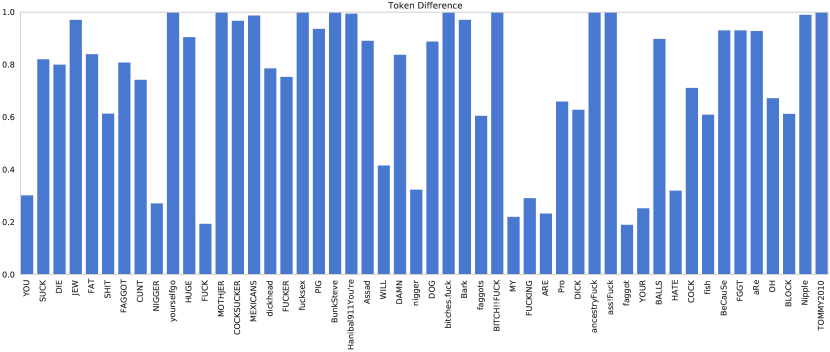
Figure 2: fraction of token occurrences (of 50 most frequent tokens) in the discarded data

Table 10 shows the preliminary explorations of the token-level distributions for the combined dataset (Section 3) with two tokenisation methods: word-level using SpaCy Honnibal and Montani (2017) and subword-level using the BPE algorithm. Based on our analysis, we draw the following conclusions: 1) token length is highly imbalanced for different datasets in Comb, particularly in Kaggle dataset⁴; 2) 99th percentile token length in Kaggle dataset⁴ is reflected in the remaining dataset. Considering this, we remove longest $1\%$ of documents from the Kaggle dataset⁴ to achieve faster computation. Through this exclusion process, the maximal token length of documents is reduced from $4950$ to $727$ tokens, without a substantial loss of information.

Model	Combined Datasets			Binary Dataset			Multi-class Dataset
	bs	client_lr	$\mu$	bs	client_lr	$\mu$	bs	client_lr	$\mu$
LogReg	$128$	$0.01$	$0.01$	$64$	$0.01$	$0.01$	$64$	$0.01$	$0.01$
Bi-LSTM	$128$	$0.001$	$0.01$	$64$	$0.001$	$0.01$	$64$	$0.001$	$0.01$
FNet	$32$	$0.0001$	$0.1$	$32$	$0.0001$	$0.001$	$32$	$0.0001$	$0.001$
DistilBERT	$32$	$0.00004$	$0.01$	$32$	$0.00002$	$0.01$	$32$	$0.00002$	$0.01$
RoBERTa	$16$	$0.00002$	$0.01$	$24$	$0.00002$	$0.01$	$32$	$0.00002$	$0.01$

Table 11: Model hyper-parameters for server-based and federated models for the Vidgen et al. (2021). ‘bs’ represents batch size, ‘client_lr’ represents client learning rate, $\mu$ represents proximal term for FedProx algorithm.

Model	Combined Datasets			Binary Dataset			Multi-class Dataset
	bs	client_lr	server_lr	bs	client_lr	server_lr	bs	client_lr	server_lr
LogReg	$128$	$0.01$	$0.01$	$64$	$0.01$	$0.001$	$64$	$0.01$	$0.01$
Bi-LSTM	$128$	$0.001$	$0.01$	$64$	$0.001$	$0.001$	$64$	$0.001$	$0.001$
FNet	$32$	$0.0001$	$0.001$	$32$	$0.0001$	$0.0001$	$32$	$0.0001$	$0.0001$
DistilBERT	$32$	$0.00004$	$0.001$	$32$	$0.00002$	$0.0001$	$32$	$0.00002$	$0.0001$
RoBERTa	$16$	$0.00002$	$0.001$	$24$	$0.00002$	$0.0001$	$32$	$0.00002$	$0.0001$

Table 12: Model hyper-parameters for server-based and federated models for the Vidgen et al. (2021). ‘bs’ represents batch size, ‘client_lr’ represents client learning rate, ‘server_lr’ represents server learning rate for FedOpt algorithm.

References

- Basile et al. (2019) Valerio Basile, Cristina Bosco, Elisabetta Fersini, Debora Nozza, Viviana Patti, Francisco Manuel Rangel Pardo, Paolo Rosso, and Manuela Sanguinetti. 2019. SemEval-2019 task 5: Multilingual detection of hate speech against immigrants and women in Twitter. In Proceedings of the 13th International Workshop on Semantic Evaluation, pages 54–63, Minneapolis, Minnesota, USA. Association for Computational Linguistics.
- Basu et al. (2021) Priya Basu, Tiasa Singha Roy, Rakshit Naidu, Zumrut Muftuoglu, Sahib Singh, and Fatemehsadat Mireshghallah. 2021. Benchmarking differential privacy and federated learning for bert models. ArXiv, abs/2106.13973.
- Bhowmick et al. (2018) Abhishek Bhowmick, John Duchi, Julien Freudiger, Gaurav Kapoor, and Ryan Rogers. 2018. Protection against reconstruction and its applications in private federated learning. arXiv preprint arXiv:1812.00984.
- Biewald (2020) Lukas Biewald. 2020. Experiment tracking with weights and biases. Software available from wandb.com.
- Crawford and Gillespie (2016) Kate Crawford and Tarleton Gillespie. 2016. What is a flag for? Social media reporting tools and the vocabulary of complaint. New Media & Society, 18(3):410–428.
- Davidson et al. (2017) Thomas Davidson, Dana Warmsley, Michael Macy, and Ingmar Weber. 2017. Automated Hate Speech Detection and the Problem of Offensive Language. In Proceedings of the International AAAI Conference on Web and Social Media. ArXiv: 1703.04009.
- de Gibert et al. (2018) Ona de Gibert, Naiara Perez, Aitor García-Pablos, and Montse Cuadros. 2018. Hate speech dataset from a white supremacy forum. In Proceedings of the 2nd Workshop on Abusive Language Online (ALW2), pages 11–20, Brussels, Belgium. Association for Computational Linguistics.
- Duchi et al. (2010) John C. Duchi, Elad Hazan, and Yoram Singer. 2010. Adaptive subgradient methods for online learning and stochastic optimization. In COLT 2010 - The 23rd Conference on Learning Theory, Haifa, Israel, June 27-29, 2010, pages 257–269. Omnipress.
- Fersini et al. (2018) Elisabetta Fersini, Debora Nozza, and Paolo Rosso. 2018. Overview of the evalita 2018 task on automatic misogyny identification (ami). EVALITA Evaluation of NLP and Speech Tools for Italian, 12:59.
- Fortuna et al. (2020) Paula Fortuna, Juan Soler, and Leo Wanner. 2020. Toxic, hateful, offensive or abusive? what are we really classifying? an empirical analysis of hate speech datasets. In Proceedings of the 12th Language Resources and Evaluation Conference, pages 6786–6794, Marseille, France. European Language Resources Association.
- Fortuna et al. (2021) Paula Fortuna, Juan Soler-Company, and Leo Wanner. 2021. How well do hate speech, toxicity, abusive and offensive language classification models generalize across datasets? Information Processing & Management, 58(3):102524.
- Founta et al. (2018) Antigoni Maria Founta, Constantinos Djouvas, Despoina Chatzakou, Ilias Leontiadis, Jeremy Blackburn, Gianluca Stringhini, Athena Vakali, Michael Sirivianos, and Nicolas Kourtellis. 2018. Large scale crowdsourcing and characterization of twitter abusive behavior. In Twelfth International AAAI Conference on Web and Social Media.
- Gandhi et al. (2022) Deep Gandhi, Jash Mehta, Nirali Parekh, Karan Waghela, Lynette D’Mello, and Zeerak Talat. 2022. A federated approach to predicting emojis in Hindi tweets. In Proceedings of the 2022 Conference on Empirical Methods in Natural Language Processing, pages 11951–11961, Abu Dhabi, United Arab Emirates. Association for Computational Linguistics.
- Ge et al. (2020) Suyu Ge, Fangzhao Wu, Chuhan Wu, Tao Qi, Yongfeng Huang, and Xing Xie. 2020. Fedner: Privacy-preserving medical named entity recognition with federated learning. arXiv preprint arXiv:2003.09288.
- Gitelman (2013) Lisa Gitelman, editor. 2013. "Raw data" is an oxymoron. Infrastructures series. The MIT Press, Cambridge, Massachusetts ; London, England.
- Hitaj et al. (2017) Briland Hitaj, Giuseppe Ateniese, and Fernando Perez-Cruz. 2017. Deep models under the gan: information leakage from collaborative deep learning. In Proceedings of the 2017 ACM SIGSAC conference on computer and communications security, pages 603–618.
- Hochreiter and Schmidhuber (1997) Sepp Hochreiter and Jürgen Schmidhuber. 1997. Long short-term memory. Neural Computation, 9(8):1735–1780.
- Honnibal and Montani (2017) Matthew Honnibal and Ines Montani. 2017. spaCy 2: Natural language understanding with Bloom embeddings, convolutional neural networks and incremental parsing.
- Karan and Šnajder (2018) Mladen Karan and Jan Šnajder. 2018. Cross-Domain Detection of Abusive Language Online. In Proceedings of the 2nd Workshop on Abusive Language Online (ALW2), pages 132–137, Brussels, Belgium. Association for Computational Linguistics.
- Kaye (2019) David Kaye. 2019. Speech police: the global struggle to govern the Internet. Columbia Global Reports.
- Kingma and Ba (2015) Diederik P. Kingma and Jimmy Ba. 2015. Adam: A method for stochastic optimization. In 3rd International Conference on Learning Representations, ICLR 2015, San Diego, CA, USA, May 7-9, 2015, Conference Track Proceedings.
- Lang (1995) Ken Lang. 1995. Newsweeder: Learning to filter netnews. In Proceedings of the Twelfth International Conference on Machine Learning, pages 331–339.
- Lee-Thorp et al. (2022) James Lee-Thorp, Joshua Ainslie, Ilya Eckstein, and Santiago Ontanon. 2022. FNet: Mixing tokens with Fourier transforms. In Proceedings of the 2022 Conference of the North American Chapter of the Association for Computational Linguistics: Human Language Technologies, pages 4296–4313, Seattle, United States. Association for Computational Linguistics.
- Li et al. (2020) Tian Li, Anit Kumar Sahu, Manzil Zaheer, Maziar Sanjabi, Ameet Talwalkar, and Virginia Smith. 2020. Federated optimization in heterogeneous networks. Proceedings of Machine learning and systems, 2:429–450.
- Lin et al. (2022) Bill Yuchen Lin, Chaoyang He, Zihang Ze, Hulin Wang, Yufen Hua, Christophe Dupuy, Rahul Gupta, Mahdi Soltanolkotabi, Xiang Ren, and Salman Avestimehr. 2022. FedNLP: Benchmarking federated learning methods for natural language processing tasks. In Findings of the Association for Computational Linguistics: NAACL 2022, pages 157–175, Seattle, United States. Association for Computational Linguistics.
- Liu and Miller (2020) Dianbo Liu and Tim Miller. 2020. Federated pretraining and fine tuning of bert using clinical notes from multiple silos. arXiv preprint arXiv:2002.08562.
- Liu et al. (2019) Yinhan Liu, Myle Ott, Naman Goyal, Jingfei Du, Mandar Joshi, Danqi Chen, Omer Levy, Mike Lewis, Luke Zettlemoyer, and Veselin Stoyanov. 2019. Roberta: A robustly optimized bert pretraining approach. arXiv preprint arXiv:1907.11692.
- McMahan et al. (2017) Brendan McMahan, Eider Moore, Daniel Ramage, Seth Hampson, and Blaise Aguera y Arcas. 2017. Communication-efficient learning of deep networks from decentralized data. In Artificial intelligence and statistics, pages 1273–1282. PMLR.
- Melis et al. (2019) Luca Melis, Congzheng Song, Emiliano De Cristofaro, and Vitaly Shmatikov. 2019. Exploiting unintended feature leakage in collaborative learning. In 2019 IEEE Symposium on Security and Privacy (SP), pages 691–706. IEEE.
- Nobata et al. (2016) Chikashi Nobata, Joel R. Tetreault, Achint Thomas, Yashar Mehdad, and Yi Chang. 2016. Abusive language detection in online user content. In Proceedings of the 25th International Conference on World Wide Web, WWW 2016, Montreal, Canada, April 11 - 15, 2016, pages 145–153. ACM.
- Park and Fung (2017) Ji Ho Park and Pascale Fung. 2017. One-step and two-step classification for abusive language detection on Twitter. In Proceedings of the First Workshop on Abusive Language Online, pages 41–45, Vancouver, BC, Canada. Association for Computational Linguistics.
- Paszke et al. (2019) Adam Paszke, Sam Gross, Francisco Massa, Adam Lerer, James Bradbury, Gregory Chanan, Trevor Killeen, Zeming Lin, Natalia Gimelshein, Luca Antiga, and et al. 2019. PyTorch: An Imperative Style, High-Performance Deep Learning Library, page 8024–8035. Curran Associates, Inc.
- Pew Research Center (2021) Pew Research Center. 2021. The State of Online Harassment. Technical report.
- Priyanshu and Naidu (2021) Aman Priyanshu and Rakshit Naidu. 2021. Fedpandemic: A cross-device federated learning approach towards elementary prognosis of diseases during a pandemic. arXiv preprint arXiv:2104.01864.
- Ramaswamy et al. (2019) Swaroop Ramaswamy, Rajiv Mathews, Kanishka Rao, and Françoise Beaufays. 2019. Federated learning for emoji prediction in a mobile keyboard. arXiv preprint arXiv:1906.04329.
- Reddi et al. (2021) Sashank J. Reddi, Zachary Charles, Manzil Zaheer, Zachary Garrett, Keith Rush, Jakub Konečný, Sanjiv Kumar, and Hugh Brendan McMahan. 2021. Adaptive federated optimization. In 9th International Conference on Learning Representations, ICLR 2021, Virtual Event, Austria, May 3-7, 2021. OpenReview.net.
- Röttger et al. (2021) Paul Röttger, Bertie Vidgen, Dong Nguyen, Zeerak Waseem, Helen Margetts, and Janet Pierrehumbert. 2021. HateCheck: Functional tests for hate speech detection models. In Proceedings of the 59th Annual Meeting of the Association for Computational Linguistics and the 11th International Joint Conference on Natural Language Processing (Volume 1: Long Papers), pages 41–58, Online. Association for Computational Linguistics.
- Sanh et al. (2019) Victor Sanh, Lysandre Debut, Julien Chaumond, and Thomas Wolf. 2019. Distilbert, a distilled version of bert: smaller, faster, cheaper and lighter. arXiv preprint arXiv:1910.01108.
- Shokri and Shmatikov (2015) Reza Shokri and Vitaly Shmatikov. 2015. Privacy-preserving deep learning. In Proceedings of the 22nd ACM SIGSAC conference on computer and communications security, pages 1310–1321.
- Swamy et al. (2019a) Steve Durairaj Swamy, Anupam Jamatia, and Björn Gambäck. 2019a. Studying generalisability across abusive language detection datasets. In Proceedings of the 23rd Conference on Computational Natural Language Learning (CoNLL), pages 940–950, Hong Kong, China. Association for Computational Linguistics.
- Swamy et al. (2019b) Steve Durairaj Swamy, Anupam Jamatia, and Björn Gambäck. 2019b. Studying Generalisability across Abusive Language Detection Datasets. In Proceedings of the 23rd Conference on Computational Natural Language Learning (CoNLL), pages 940–950, Hong Kong, China. Association for Computational Linguistics.
- Talat and Hovy (2016) Zeerak Talat and Dirk Hovy. 2016. Hateful Symbols or Hateful People? Predictive Features for Hate Speech Detection on Twitter. In Proceedings of the NAACL Student Research Workshop, pages 88–93, San Diego, California. Association for Computational Linguistics.
- Thylstrup and Talat (2020) Nanna Thylstrup and Zeerak Talat. 2020. Detecting ‘Dirt’ and ‘Toxicity’: Rethinking Content Moderation as Pollution Behaviour. SSRN Electronic Journal.
- Vidgen et al. (2021) Bertie Vidgen, Tristan Thrush, Zeerak Waseem, and Douwe Kiela. 2021. Learning from the worst: Dynamically generated datasets to improve online hate detection. In Proceedings of the 59th Annual Meeting of the Association for Computational Linguistics and the 11th International Joint Conference on Natural Language Processing (Volume 1: Long Papers), pages 1667–1682, Online. Association for Computational Linguistics.
- Wolf et al. (2020) Thomas Wolf, Lysandre Debut, Victor Sanh, Julien Chaumond, Clement Delangue, Anthony Moi, Pierric Cistac, Tim Rault, Remi Louf, Morgan Funtowicz, Joe Davison, Sam Shleifer, Patrick von Platen, Clara Ma, Yacine Jernite, Julien Plu, Canwen Xu, Teven Le Scao, Sylvain Gugger, Mariama Drame, Quentin Lhoest, and Alexander Rush. 2020. Transformers: State-of-the-art natural language processing. In Proceedings of the 2020 Conference on Empirical Methods in Natural Language Processing: System Demonstrations, pages 38–45, Online. Association for Computational Linguistics.
- Yang et al. (2018) Timothy Yang, Galen Andrew, Hubert Eichner, Haicheng Sun, Wei Li, Nicholas Kong, Daniel Ramage, and Françoise Beaufays. 2018. Applied federated learning: Improving google keyboard query suggestions. arXiv preprint arXiv:1812.02903.
- Zampieri et al. (2019) Marcos Zampieri, Shervin Malmasi, Preslav Nakov, Sara Rosenthal, Noura Farra, and Ritesh Kumar. 2019. Predicting the type and target of offensive posts in social media. In Proceedings of the 2019 Conference of the North American Chapter of the Association for Computational Linguistics: Human Language Technologies, Volume 1 (Long and Short Papers), pages 1415–1420, Minneapolis, Minnesota. Association for Computational Linguistics.