Collapsars as Sites of r-process Nucleosynthesis: Systematic Photometric Near-Infrared Follow-up of Type Ic-BL Supernovae

Abstract

One of the open questions following the discovery of GW170817 is whether neutron star mergers are the only astrophysical sites capable of producing r-process elements. Simulations have shown that 0.01-0.1M_⊙ of r-process material could be generated in the outflows originating from the accretion disk surrounding the rapidly rotating black hole that forms as a remnant to both neutron star mergers and collapsing massive stars associated with long-duration gamma-ray bursts (collapsars). The hallmark signature of r-process nucleosynthesis in the binary neutron star merger GW170817 was its long-lasting near-infrared emission, thus motivating a systematic photometric study of the light curves of broadlined stripped-envelope (Ic-BL) supernovae (SNe) associated with collapsars. We present the first systematic study of 25 SNe Ic-BL—including 18 observed with the Zwicky Transient Facility and 7 from the literature—in the optical/near-infrared bands to determine what quantity of r-process material, if any, is synthesized in these explosions. Using semi-analytic models designed to account for r-process production in SNe Ic-BL, we perform light curve fitting to derive constraints on the r-process mass for these SNe. We also perform independent light curve fits to models without r-process. We find that the r-process-free models are a better fit to the light curves of the objects in our sample. Thus we find no compelling evidence of r-process enrichment in any of our objects. Further high-cadence infrared photometric studies and nebular spectroscopic analysis would be sensitive to smaller quantities of r-process ejecta mass or indicate whether all collapsars are completely devoid of r-process nucleosynthesis.

1 Introduction

The dominant process responsible for producing elements heavier than iron is the rapid neutron capture process, known as the r-process (Burbidge et al., 1957; Cameron, 1957), which only has a few plausible astrophysical sites. While standard core-collapse supernovae (SNe) were previously considered as candidate sites for r-process nucleosynthesis (Woosley et al., 1994; Takahashi et al., 1994; Qian & Woosley, 1996), they have since been disfavored because simulations of neutrino-driven winds in core-collapse SNe fail to create conducive conditions for r-process production (Thompson et al., 2001; Roberts et al., 2010; Martínez-Pinedo et al., 2012; Hotokezaka et al., 2018). On the other hand, before 2017, many studies (Lattimer & Schramm, 1974, 1976; Symbalisty & Schramm, 1982) predicted that mergers of two neutron stars (NSs) or neutron stars with black holes were capable of generating r-process elements during the decompression of cold, neutron-rich matter ensuing from the tidal disruption of the neutron stars. Li & Paczyński (1998) first suggested that the signature of such r-process nucleosynthesis would be detectable in an ultraviolet, optical and near-infrared (NIR) transient powered by the radioactive decay of neutron-rich nuclei, termed as a “kilonova” for its brightness, which was predicted to be 1000$\times$ that of a classical nova (Metzger et al., 2010). Other studies proposed that r-process elements could be synthesized in a rare SN subtype known as a hypernova (e.g. Fujimoto et al., 2007). In this scenario, the SN explosion produces a rapidly rotating central BH surrounded by an accretion disk. Accretion onto the BH is thought to power a relativistic jet, while material in the disk may neutronize, allowing the r-process to occur when the newly neutron-rich material is unbound as a disk wind.

Galactic archaeological studies (Ji et al., 2016a, b), geochemical studies (Wallner et al., 2021), and studies of the early solar system (Tissot et al., 2016) offer unique insights into which astrophysical sites could plausibly explain observed r-process elemental abundances. A recent study of r-process abundances in the Magellanic Clouds indicate that the astrophysical r-process site has a time-delay longer than for core-collapse SNe (Reggiani et al., 2021). Second- and third-peak abundance patterns inferred from metal-poor Galactic halo stars show consistency with the solar r-process abundance pattern at high atomic number, but scatter at low atomic number that could be attributed to enrichment from multiple sources, including magneto-rotational hypernovae (Yong et al., 2021). Measurements of excess $[\rm Ba/Fe]$ and $[\rm Eu/Fe]$ abundances in the dwarf galaxy Reticulum II argue for not only a rare and prolific event, but one capable of enriching the galaxy early in its history (Ji et al., 2016a; Tarumi et al., 2020), pointing towards a potential rare SN subtype whose r-process production would follow star formation (Côté et al., 2019; Siegel et al., 2019). Further evidence of heavy r-process enrichment in the disrupted dwarf galaxy Gaia Sausage Enceladus ($\sim$3.6 Gyr star formation duration) but not in the disrupted dwarf galaxy Kraken (with $\approx$2 Gyr star formation duration) points towards multiple r-process enrichment sites operating on different timescales (Naidu et al., 2021).

Overall, geological studies and studies of the early solar system and Galactic chemical evolution exemplify the need for rare and prolific astrophysical sites to explain observed abundances, and insinuate that the solar r-process abundance pattern could be universal. While NS mergers are compatible with many facets of the above findings (Hotokezaka et al., 2018; Côté et al., 2018; Metzger, 2019), assuming that mergers are the sole producers of r-process material presents some potential hurdles. For example, the time delay between formation and merger of NS systems must be short enough to enrich old, ultra-faint dwarf galaxies with heavy elements (Roederer et al., 2016; Ji et al., 2016a; Côté et al., 2019). Furthermore, natal merger kicks present a challenge for low-mass galaxies to retain pre-merger compact binaries (Komiya & Shigeyama, 2016). The question of whether NS mergers alone can explain the relative abundances of r-process elements (e.g. $[\rm Eu/Fe]$ vs. $[\rm Fe/H]$) in the solar neighborhood remains unanswered (Beniamini et al., 2016; Bonetti et al., 2019).

The multi-messenger detection of the binary neutron star merger GW170817 (Abbott et al., 2017a), an associated short burst of gamma-rays GRB170817 (Abbott et al., 2017b) and the kilonova AT2017gfo (Andreoni et al., 2017; Chornock et al., 2017a; Coulter et al., 2017; Cowperthwaite et al., 2017; Drout et al., 2017; Evans et al., 2017; Kasliwal et al., 2017, 2022; Kilpatrick et al., 2017; Lipunov et al., 2017; McCully et al., 2017; Nicholl et al., 2017; Shappee et al., 2017; Soares-Santos et al., 2017; Pian et al., 2017; Smartt et al., 2017; Tanvir et al., 2017; Villar et al., 2017; Utsumi et al., 2017) relayed the first direct evidence that NS mergers are an astrophysical site of r-process nucleosynthesis and short GRB progenitors. Multi-band photometry and optical/NIR spectroscopy of AT2017gfo indicated that the KN ejecta was enriched with r-process elements (Drout et al., 2017; Chornock et al., 2017b; Cowperthwaite et al., 2017; Kasliwal et al., 2017; Kilpatrick et al., 2017; Pian et al., 2017; Smartt et al., 2017; Tanvir et al., 2017; Watson et al., 2019) including heavier species occupying the second- and third-peak (Tanvir et al., 2017; Watson et al., 2019; Kasliwal et al., 2022; Gillanders et al., 2021).

Although GW170817 confirmed NS mergers as r-process nucleosynthesis sites, some fundamental open questions on the nature of r-process production still remain. Namely, can the rates of and expected yields from NS mergers explain the total amount of r-process production measured in the Universe? Or, do the direct and indirect clues about r-process production in the Universe point towards an alternative r-process site, such as rare core-collapse SNe?

The discovery of the broadlined Type Ic supernova SN 1998bw at 40 Mpc (Galama et al., 1998), following the long GRB 980425 was a watershed event that provided the first hints that some GRBs were connected to stellar explosions (Kulkarni et al., 1998; Galama et al., 1999). However, due to the anomalous nature of the explosion, it was not until GRB 030329 that a direct long GRB–SN connection was securely established (Fynbo et al., 2004). The spectra of these SNe exhibit broad features due to high photospheric velocities (${\gtrsim}20,000$ km s^-1). They have higher inferred kinetic energies than typical SNe (at $\sim$10⁵² erg), and are stripped of both hydrogen and helium (Modjaz et al., 2016; Gal-Yam, 2017). Since SN 1998bw, several other SNe Ic-BL have been discovered in conjunction with long GRBs (e.g. Kocevski et al. 2007; Olivares E. et al. 2012; Cano et al. 2017b; Corsi & Lazzati 2021), boosting the existing collapsar theory (Woosley, 1993; MacFadyen & Woosley, 1999; MacFadyen et al., 2001) as a mechanism to explain long GRBs and their associated SN counterparts. The term collapsar refers to a rapidly-rotating, massive star that collapses into a black hole, forming an accretion disk around the central black hole. Collapsars are distinct from the magnetar-powered explosions (referred to as “magnetohydrodynamic (MHD) SNe”) also proposed to be related to SNe Ic-BL (Metzger et al., 2011; Kashiyama et al., 2016). However, puzzling discoveries including that of GRB060505 and GRB060614 which lacked a clear SN counterpart to deep limits (Gehrels et al., 2006) and that of GRB211211A, a long-duration GRB associated with a kilonova (Rastinejad et al., 2022) have shifted the paradigm from the traditional conception that all long GRBs have a collapsar or magnetar origin. Thus some fraction of long-duration GRBs may also originate from compact binary mergers.

Several works (Fujimoto et al., 2007; Ono et al., 2012; Nakamura et al., 2015; Soker & Gilkis, 2017) have since hypothesized that the explosions that give rise to SNe Ic-BL and (in some cases) to their accompanying long GRBs (i.e. collapsars) are capable of producing 0.01-0.1M_⊙ of r-process material per event. Simulations suggest that in the case of a NS merger, an accretion disk forms surrounding the merger’s newly-born central black hole (Shibata & Taniguchi, 2006) and r-process elements originate in the associated disk outflows (Metzger et al., 2008, 2009). Such accretion flows are not only central to the short GRBs associated with NS mergers, but also with the long classes of GRBs associated with collapsars. However, predictions about r-process-production in the collapsar context are sensitive to assumptions about the magnetic field, the disk viscosity model, and the treatment of neutrinos, among other factors. Surman et al. (2006) argued that only light r-process elements can be synthesized in collapsar accretion disks due to neutrino-driven winds. More recently, Siegel et al. (2019) conducted 3D general-relativistic, magnetohydrodynamic simulations demonstrating sufficient r-process yields to explain the observed abundances in the Universe. Siegel et al. (2019) found that the disk material becomes neutron-rich through weak interactions, enabling the production of even 2nd and 3rd peak r-process elements in disk-wind outflows. Other works in the literature (Miller et al., 2020; Just et al., 2022; Fujibayashi et al., 2022) have argued that collapsars are inefficient producers of r-process elements based on studies of the full radiation transport and $\alpha$-viscosity in collapsar disks. Whether or not collapsars are sites of r-process nucleosynthesis is still an active area of investigation, motivating detailed studies of the photometric evolution of r-process enriched SNe.

Recently, Barnes & Metzger (2022), motivated by Siegel et al. (2019), created semi-analytic models of the light curves of SNe from collapsars producing r-process elements, yielding concrete predictions for the photometric evolution of r-process-enriched SNe Ic-BL. Our work is focused on observationally testing the models from Barnes & Metzger (2022).

In this work, we report our findings from an extensive observational campaign and compilations from the literature to determine whether collapsars powering SNe Ic-BL are capable of synthesizing r-process elements. We present optical and near-infrared photometric observations and compare both color evolution and absolute light curves against the predictions from Barnes & Metzger (2022). Our paper is structured as follows: First, we detail our sample selection criteria in Sec. 2, then Sec. 3 describes our optical and NIR observations, followed by Sec. 4 which provides the discovery details about each candidate. Sec. 5 introduces the objects from the literature used in our study, and in Sec. 6 we introduce the latest collapsar r-process models. In Sec. 7, we show how we derive explosion properties. The results of our light curve model fits are presented in Sec. 8, and finally we discuss our conclusions and future work in Sec. 9.

2 Sample Selection

To test the hypothesis that SNe Ic-BL generate r-process elements, we require a statistically robust sample size of SNe with contemporaneous NIR and optical light curves. To obtain optical light curves, we use data from the Zwicky Transient Facility (ZTF; Bellm et al. 2019; Masci et al. 2019; Graham et al. 2019), a 47 sq. deg. field-of-view mosaic camera with a pixel scale of 1$\arcsec$/pixel (Dekany et al., 2020) installed on the Palomar 48 in. telescope. ZTF images the entire Northern sky every $\sim$2 nights in g- and $r-$bands, attaining a median 5$\sigma$ detection depth of 20.5 m_AB. Amongst the systematic efforts aimed at SN detection with ZTF, our SNe draw from two surveys in particular: “Bright Transient Survey” (BTS; Fremling et al. 2020) and the ZTF “Census of the Local Universe” survey (CLU; De et al. 2020) which are conducted as a part of ZTF’s nightly operations. BTS is a magnitude-limited survey aimed at spectroscopically classifying all SNe $<18.5$ mag at peak brightness (Perley et al., 2020). CLU, in contrast, is a volume-limited survey aimed at classifying all SNe within 150 Mpc whose hosts belong to the CLU galaxy catalog (Cook et al., 2019). The CLU galaxy catalog is designed to provide spectroscopic redshifts of all galaxies within 200 Mpc, and is 90% complete (for an H$\alpha$ line flux of 4$\times 10^{-14}$ erg cm² s^-1). Hence the two surveys provide complementary methods for SN identification. Our sample consists of 18 spectroscopically-confirmed ZTF SNe Ic-BL within $z\lesssim 0.05$. Due to our low redshift cut, we assume that the photometric K-corrections are negligible (Taddia et al., 2018). The details of the instruments and configurations used to take our classification spectra are described in Sec. 3 (see also Fig. 1). Where available, we use the spectroscopic redshift from the SDSS galaxy host (especially for sources falling in the CLU sample) and otherwise determine the SN redshift from spectral fitting to the narrow galaxy H$\alpha$ feature. For each spectrum, we use the Supernova Identification code (SNID; Blondin & Tonry 2007) to determine the best match template (also plotted in Fig. 1), fixing the redshift to the value determined using the methods described above. We overplot the characteristic spectroscopic lines for SNe Ic-BL including O I, Fe II, and Si II in dashed lines, along with Na I D, an indicator of the amount of supernova host galaxy extinction (Stritzinger et al., 2018a). For all of the ZTF SNe, we assume zero host attenuation; this assumption is backed by the lack of any prominent Na I D absorption features in the spectra (see Fig. 1). Higher host attenuation results in redder observed SN colors.

We impose a redshift cut to eliminate distant SNe that might fade rapidly below ZTF detection limits within 60 days post-peak. ZTF yields an average rate of SNe Ic-BL discovery of $\sim$1/month, but due to visibility and weather losses, we followed-up $\sim$10 SNe per year. As a consequence of our sample selection from ZTF, probing only the local volume, we are biased against GRB-SNe. However, amongst our sample, we include one LLGRB (GRB190829A), SN 2018gep, a published SN with fast and luminous emission (Ho et al., 2019), and another published SN with a mildly-relativistic ejecta, SN 2020bvc (Ho et al., 2020a), which contribute diversity to our ZTF sample. The two SNe exhibited broad features in their spectra and were classified as SNe Ic-BL, while the LLGRB was too faint for spectroscopy, and only had photometric evidence of an associated SN bump.

In the analyses in subsequent sections, we assume the following cosmological parameters: H${}_{0}=63.7\rm km\,s^{-1}\,Mpc^{-1}$, $\Omega_{m}=0.307$.

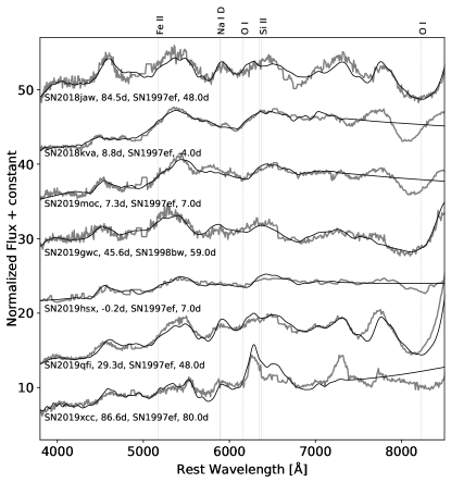
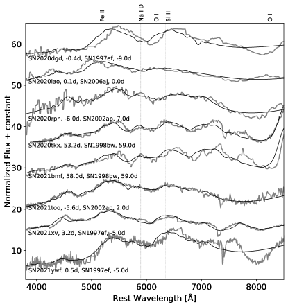
Figure 1: Classification spectra for the SNe Ic-BL in our sample, along with their SNID best-match templates, labeled by name, supernova phase relative to the peak light, and corresponding template name, and template phase from SNID. GRB190829A only has a host spectrum, which we do not display here. The spectra for SN 2018gep and SN 2020bvc are published in Ho et al. (2019) and Ho et al. (2020a) so we do not show them here. The spectra show broad Fe II, Si II and O I lines. The Na I D absorption line, an indicator of host extinction (Stritzinger et al., 2018a), is plotted for reference – none of the SNe appear to have strong Na I D features.

3 Observations

Here we describe the photometric and spectroscopic observations obtained by various facilities in our follow-up campaign.

3.1 Photometry

3.1.1 ZTF

We use the ZTF camera on the Palomar 48-in telescope for supernova discovery and initial follow-up. ZTF’s default observing mode consists of 30 s exposures. Alerts (5$\sigma$ changes in brightness relative to the reference image) are disseminated in avro format (Patterson et al., 2019) and filtered based on machine-learning real-bogus classifiers (Mahabal et al., 2019), star-galaxy classifiers (Tachibana & Miller, 2018), and light curve properties. Cross-matches with solar-system objects serve to reject asteroids. ZTF’s survey observations automatically obtain $r-$, $g-$ and sometimes $i-$ band imaging lasting $\approx$60 days after peak, while the supernova is brighter than 20.5 mag. Masci et al. (2019) provides more information about the data processing and image subtraction pipelines. More details about specific surveys used to obtain these data are provided in Sec 2.

3.1.2 LCOGT

We performed photometric follow-up of our SNe with the Sinistro and Spectral cameras on the Las Cumbres Observatory Global Telescope (LCOGT; Brown et al. 2013) Network’s 1-m and 2-m telescopes respectively. The Sinistro (Spectral) camera has a field of view of 26.5 (10.5)$\arcmin$ x 26.5 (10.5)$\arcmin$ and a pixel scale of 0.389 (0.304)$\arcsec$/pixel. The observations relied on two separate LCO programs: one aimed at supplementing ZTF light curves of Bright Transient Survey objects and the other intending to acquire late-time $r-$ and $i-$ band follow-up of stripped-envelope SNe fainter than 21 mag. The exposure times and number of images requested varied based on filter and desired depth, ranging from 160 s to 300 s and from 1 to 5 images. The data are automatically flat-fielded and bias-subtracted. Though both programs use different data reduction pipelines, the methodology is nearly the same. Both pipelines extract sources using the Source Extractor package (Bertin & Arnouts, 2010) and calibrate magnitudes against Pan-STARRS1 (PS1) (Chambers et al., 2016; Flewelling, 2018) objects in the vicinity. The BTS-targeted program uses the High Order Transform of Psf ANd Template Subtraction code (HOTPANTS; Becker 2015) to subtract a PSF scaled Pan-STARRS1 template previously aligned using SCAMP (Bertin, 2006). For the late-time LCOGT follow-up program, our pipeline performed image subtraction with pyzogy (Guevel & Hosseinzadeh, 2017), based on the ZOGY algorithm (Zackay et al., 2016). Both pipelines stack multiple images to to increase depth.

3.1.3 WASP

We performed deep imaging with the WAfer-scale imager for Prime (WASP), mounted on the Palomar 200-in. prime focus with a 18.5$\arcmin$ x 18.5$\arcmin$ field of view and a plate scale of 0.18$\arcsec$/pixel. We obtained data from WASP for the transients at late times in the $g^{\prime}-$, $r^{\prime}-$ and $i^{\prime}-$ filters. The data were reduced using a python based pipeline that applied standard optical reduction techniques (as described in De et al. 2020), and the photometric calibration was obtained against PS1 sources in the field. Image subtraction was performed with HOTPANTS with references from PS1 and SDSS.

3.1.4 SEDM

We obtained additional photometric follow-up with the Spectral Energy Distribution Machine (SEDM; Blagorodnova et al. 2018; Rigault et al. 2019; Kim et al. 2022) on the Palomar 60-inch (P60) telescope which has a field of view of 13$\arcmin$ x 13$\arcmin$ and a plate scale of 0.378$\arcsec$/pixel. The processing is automated, and can be triggered using the Fritz marshal (Kasliwal et al., 2019; Duev et al., 2019; van der Walt et al., 2019). Standard imaging requests involve $g-$, $r-$, and $i-$ band 300s exposures with the Rainbow Camera on SEDM. The data are later reduced using a python-based pipeline that applies standard reduction techniques and applies a customized version of FPipe (Fremling Automated Pipeline; Fremling et al. 2016) for image subtraction.

3.1.5 Liverpool IO:O

We acquired late-time, multi-band imaging with the Liverpool Telescope (Steele et al., 2004) using the IO:O camera with the Sloan $griz$ filter set. The IO:O camera has a 10$\arcmin$x10$\arcmin$ field of view with a plate scale of 0.15$\arcsec$/pixel. An automatic pipeline reduces the images, performing bias subtraction, trimming of the overscan regions, and flat fielding. Once a PS1 template is aligned, the image subtraction takes place, and the final photometry comes from the analysis of the subtracted image.

3.1.6 GROWTH-India Telescope

We obtained photometric follow-up of our SNe with the 0.7m robotic GROWTH-India Telescope (GIT; Kumar et al. 2022) equipped with a 4096×4108 pixel back-illuminated Andor camera. GIT has a circular field of view of 0.86$\deg$ x 0.86 $\deg$ (corresponding to 51.6$\arcmin$ x 51.6$\arcmin$) and has a pixel scale of 0.676$\arcsec$/pixel. GIT is located at the IAO (Hanle, Ladakh). Targeted observations were conducted in SDSS $r^{\prime},\text{and}\,i^{\prime}$ filters with varying exposure times. All data were downloaded in real time and processed with the automated GIT pipeline. Zero points for photometry were calculated using the PanSTARRS catalogue (Flewelling, 2018), downloaded from Vizier (Ochsenbein et al., 2000). We performed image subtraction with pyzogy and PSF photometry with PSFEx (Bertin, 2011).

3.1.7 WIRC

We obtained near-infrared follow-up imaging of candidates with the Wide-field Infrared Camera (WIRC; Wilson et al. 2003), on the Palomar 200-inch telescope (P200) in $J-$, $H-$ and $K$-short ($Ks-$) bands. WIRC’s field of view is 8.7$\arcmin$ x 8.7$\arcmin$ with a pixel scale of 0.2487$\arcsec$/pixel. The WIRC data was reduced using the same pipeline as described above for WASP, but it was additionally stacked using Swarp (Bertin, 2010) while the calibration was done using the 2MASS point source catalog (Skrutskie et al., 2006). We obtained the WIRC data during classical observing runs on a $\sim$monthly cadence between January 2019 and December 2021. Due to the fact that the 2MASS Catalog is far shallower ($J=15.8,H=15.1,Ks=14.3$ m_AB; Skrutskie et al. 2006) compared to WIRC’s limiting magnitudes ($J=22.6,H=22.0,Ks=21.5$, in AB mag), we obtained reference images with WIRC after the SNe had faded in order to perform reference image subtraction. We perform image subtraction using the HOTPANTS algorithm and obtain aperture photometry using photutils (Bradley et al., 2020).

3.2 Spectroscopy

3.2.1 SEDM

We also used the SEDM’s low-dispersion (R$\sim$100) integral field spectrograph (IFU) to obtain classification spectra for several of our objects. The field of view is 28$\arcsec$ x 28$\arcsec$ with a pixel scale of 0.125$\arcsec$/pixel. The SEDM is fully roboticized from the request submission to data acquisition to image reduction and uploading. The IFU images are reduced using the custom SEDM IFU data reduction pipeline (Blagorodnova et al., 2018; Rigault et al., 2019), which relies on the steps flat-fielding, wavelength calibration, extraction, flux calibration, and telluric correction.

3.2.2 DBSP

We obtained low to medium resolution (R$\sim$1000-10000) classification spectra of many of the SNe in our sample with Double Spectrograph (DBSP; Oke & Gunn 1982) on the Palomar 200-in telescope. Its plate scale is 0.293$\arcsec$/pixel (red side) and 0.389 $\arcsec$/pixel (blue side) and field of view is 120$\arcsec$ x 70$\arcsec$. The setup included a red grating of 316/7500, a blue grating of 600/400, a D55 dichroic, and slitmasks of 1$\arcsec$, 1.5$\arcsec$, and 2$\arcsec$. Some of our data was reduced using a custom PyRAF DBSP reduction pipeline (Bellm & Sesar, 2016) while the rest were reduced using a custom DBSP Data Reduction pipeline relying on Pypeit (Prochaska et al., 2019; Mandigo-Stoba et al., 2022).

3.2.3 LRIS

Some of the SNe in our sample also have spectra from the Low Resolution Imaging Spectrometer (LRIS; Oke et al. 1995) mounted on the 10 m Keck I telescope. LRIS has a 6$\arcmin$ x 7.8$\arcmin$ field of view and a pixel scale of 0.135$\arcsec$/pixel. We used the 400/3400 grism on the blue arm and the 400/8500 grating on the red arm, with a central wavelength of 7830 $\rm\AA$ to cover the bandpass from 3,200-10,000 $\rm\AA$. We used longslit masks of 1.0$\arcsec$ and 1.5$\arcsec$ width. We typically used an exposure time of 600 s to obtain our classification spectra. The spectra were reduced using LPipe (Perley, 2019).

3.2.4 NOT

We obtained low-resolution spectra with the Alhambra Faint Object Spectrograph and Camera (ALFOSC) on the 2.56 m Nordic Optical Telescope (NOT) at the Observatorio del Roque de los Muchachos on La Palma (Spain). The ALFOSC has a field of view of 6.4$\arcmin$ x 6.4$\arcmin$ and a pixel scale of 0.2138$\arcsec$/pixel. The spectra were obtained with a 1$\farcs$0 wide slit and grism #4. The data were reduced with IRAF and PypeIt. The spectra were calibrated with spectrophotometric standard stars observed during the same night and the same instrument setup.

4 Description of ZTF candidates

In the section below we include descriptions of all of the 18 candidates with ZTF data that were analyzed in this paper, including details about its discovery, coincident radio and X-ray data and any other notable characteristics about the objects. Our literature sample is described in Sec. 5. Some of these candidates are part of a companion study (Corsi et al., 2023) focusing on radio properties of SNe Ic-BL; the full ZTF sample of SNe Ic-BL will be presented in Srinivasaragavan et al., in prep. For all Swift XRT fluxes reported from the companion study, we assume a spectral model of a power-law spectrum with photon index $\Gamma=2$ corrected for Galactic absorption only. The 90% flux upper limits for Swift XRT reported below are calculated by converting counts to flux using the same power-law model. All Swift fluxes have an energy range of 0.3-10 keV. For a more thorough discussion of whether the reported X-ray and radio emission correspond to transient or host-only emission, see Sections 3.4 and 3.5 of Corsi et al. (2023).

The objects described here range from M${}_{r}=-16.58$ to M${}_{r}=-20.60$ mag and from $z=0.017$ to $z=0.056$ (excluding the LLGRB, at $z=0.077$). All of the transients included below are ZTF SNe, but we hereafter refer to them by their IAU names. We performed forced photometry (using the MCMC method) for all of the candidates using ForcePhotZTF (Yao et al., 2019).

We found no coincident Fermi, Swift, MAXI, AGILE, or INTEGRAL GRB triggers or serendipitous Chandra or XMM X-ray coverage for these SNe based on their derived explosion dates. Though several candidate counterparts were found in temporal coincidence with KONUS instrument on the Wind satellite, the explosion epoch uncertainties hinder our ability to make any firm association to the KONUS sources. These objects are summarized in Tables 1, and their classification spectra are shown in Figure 1.

4.1 SN 2021ywf

Our first ZTF photometry of SN 2021ywf (ZTF21acbnfos) was obtained on 2021 September 12 ($\mathrm{MJD}=59469.47$) with the P48. This first detection was in the $r-$ band, with a host-subtracted magnitude of $20.03\pm 0.20$, at $\alpha=05^{h}14^{m}11.00^{s}$, $\delta=+01\arcdeg 52\arcmin 52.3\arcsec$ (J2000.0). The discovery was reported to TNS on 2021 September 14 (Nordin et al., 2021), with a note saying that the latest non-detection from ZTF was just 1 day prior to discovery ($r=20.2$ mag). The high cadence around discovery allows for a well constrained explosion date. With power-law fits to the early $g-$ and $r-$ band data, we estimate the explosion date as $\mathrm{MJD_{explosion}^{SN2021ywf}}=59467.70\pm 0.2$ (see below).

We classified the transient as a Type Ic-BL using a spectrum from P200+DBSP obtained on 2021 September 27 (Chu et al., 2021). The first spectrum was actually obtained using the P60+SEDM. However, the quality of that spectrum was not good enough to warrant a classification. SN 2021ywf exploded in the outskirts of the spiral galaxy CGCG 395-022 with a well established redshift of $z=0.028249$, which corresponds to a luminosity distance of 127.85 Mpc and a distance modulus of 35.534. This redshift is confirmed with narrow host lines in our classification spectrum.

On 2021 September 30, SN 2021ywf was detected (3.2$\sigma$ significance) both with the Swift XRT with $5.3_{-3.3}^{+4.9}\times 10^{-14}\rm\,erg\,cm^{-2}\,s^{-1}$ in a 7.2 ks observation, and with the VLA at $83\pm 10\,\mu$Jy at 5.0 GHz (see Corsi et al. 2023 for details).

4.2 SN 2021xv

Our first ZTF photometry of SN 2021xv (ZTF21aadatfg) was obtained on 2021 January 10 ($\mathrm{MJD}=59224.52$) with the P48. The transient was discovered in the public ZTF alert stream and reported by ALeRCE (Forster, 2021). This first detection was in the $r-$ band, with a host-subtracted magnitude of 19.93, at $\alpha=16^{h}07^{m}32.82^{s}$, $\delta=+36\arcdeg 46\arcmin 46.07\arcsec$ (J2000.0). The discovery was reported to TNS (Forster et al., 2021), with a note saying that the last non-detection was 3 days before discovery (on 2021 January 07 at $r=$19.52 mag). We classified the transient as a Type Ic-BL using a spectrum from the NOT+ALFOSC obtained on 2021 Jan 25 (Schulze & Sollerman, 2021). The transient appears to be associated with the galaxy host SDSS J160732.83+364646.1. We measure a redshift of $z=0.041$ from the narrow host lines in the NOT spectrum, corresponding to a luminosity distance of 187.29 Mpc and a distance modulus of 36.363. SN 2021xv was marginally detected with the VLA on 2021 May 19 at F${}_{\nu}=34.3\pm 8.1\,\mu$Jy at 5.2 GHz, but the detection is consistent with host galaxy emission (see Corsi et al. 2023 for details).

4.3 SN 2021too

SN 2021too (ZTF21abmjgwf) was reported first by the PS1 Young Supernova Experiment on 2021 July 17 ($\mathrm{MJD}=59412.60$) with the internal name PS21iap, but the first ZTF alerts are from 2021 July 16. This first detection was in the $i-$ band, with a host-subtracted magnitude of 19.5, at $\alpha=21^{h}40^{m}54.28^{s}$, $\delta=+10\arcdeg 19\arcmin 30.3\arcsec$ (J2000.0). The discovery was reported to TNS (Jones et al., 2021). Our last non-detection with ZTF was on 2021 July 16 at $r=20.4$ mag. The transient was classified as a Type Ic-BL using a spectrum from EFOSC2-NTT obtained on 2021 August 02 by ePESSTO (Pessi et al., 2021). The object was positioned in the starforming galaxy SDSS J214054.29+101930.5. We measure a redshift of 0.035 from the narrow host lines in its P200+DBSP spectrum taken on 2021 Aug 07. This corresponds to a luminosity distance of 159.19 Mpc and a distance modulus of 36.01.

4.4 SN 2021bmf

SN 2021bmf (ZTF21aagtpro) was discovered by ATLAS on 2021 January 30 ($\mathrm{MJD}=59244.0$) with the internal name ATLAS 21djt, and later by ZTF ($\mathrm{MJD}=59248.0$). This first detection was in the $o$ band, with a host-subtracted magnitude of 18.12, at $\alpha=16^{h}33^{m}29.41^{s}$, $\delta=-06\arcdeg 22\arcmin 49.53\arcsec$ (J2000.0). The discovery was reported to TNS (Tonry et al., 2021), with a note saying that the last non-detection was on 2021 January 16 at $c=18.4$ mag. The transient was classified as a Type Ic-BL using a spectrum from ePESSTO obtained on 2021 February 03 (Magee et al., 2021). SN 2021bmf was found in the faint host galaxy SDSS J163329.48-062249.9, which was determined to be at $z=0.0175$ based on narrow host lines in the Keck I LRIS spectrum taken on 2021 July 09, which corresponds to a luminosity distance of 78.57 Mpc and a distance modulus of 34.476.

4.5 SN 2020tkx

Our first ZTF photometry of SN 2020tkx (ZTF20abzoeiw) was obtained on 2020 September 16 ($\mathrm{MJD}=59108.26$) with the P48. This first detection was in the $g-$ band, with a host-subtracted magnitude of $18.09\pm 0.08$, at $\alpha=18^{h}40^{m}09.01^{s}$, $\delta=+34\arcdeg 06\arcmin 59.5\arcsec$ (J2000.0). The discovery was done by Gaia two days earlier (Hodgkin et al., 2020). The last ZTF non-detection is from 2021 September 07, a full week before discovery, and the constraints on the explosion date are therefore imprecise.

The transient was classified as a Type Ic-BL by Srivastav et al. (2020) based on a spectrum from the Spectrograph for the Rapid Acquisition of Transients (SPRAT) on LT, obtained on 2020 September 18. Our sequence of P60 spectra taken in 2020 confirm this classification.

SN 2020tkx exploded in a faint host galaxy without a known redshift. Using the spectral template fitting SNID for our best NOT+ALFOSC spectrum taken on 2020 November 18, the redshift can be constrained to $z\sim 0.02-0.03$, and our adopted redshift of $z=0.027$ is based on a weak, tentative H$\alpha$ line from the host galaxy in the spectrum. The adopted redshift translates to a luminosity distance of 122.09 Mpc and a distance modulus of 35.433.

The object has a upper limit of $<3.3\times 10^{-14}\rm erg\,cm^{-2}\,s^{-1}$ with the Swift XRT (8.1 ks exposure) on 2020 October 03, 8.9 days after peak light. SN 2020tkx was detected with the VLA at $286\pm 15\,\mu$Jy (10 GHz) on 2021 September 25 (see Corsi et al. 2023 for more details).

4.6 SN 2020rph

Our first ZTF photometry of SN 2020rph (ZTF20abswdbg) was obtained on 2020 August 11 ($\mathrm{MJD}=59072.49$) with the P48. The transient was discovered in the public ZTF alert stream and reported by ALeRCE. This first detection was in the r band, with a host-subtracted magnitude of 20.36, at $\alpha=03^{h}15^{m}17.82^{s}$, $\delta=+37\arcdeg 00\arcmin 50.57\arcsec$ (J2000.0). The discovery was reported to TNS (Forster et al., 2020a), with the last non-detection just 1 hour before discovery at $r=$19.88 mag. We classified the transient as a Type Ic-BL using a spectrum from the P60+SEDM obtained on 2020 August 24 (Dahiwale & Fremling, 2020a). The supernova was found offset from the galaxy WISEA J031517.67+370055.3. We measure a redshift of $z=0.042$ based on a Keck I LRIS spectrum taken on 2020 October 19, which corresponds to a luminosity distance of 192.0 Mpc and a distance modulus of 36.42. SN 2020rph has a Swift XRT upper limit of f$<3.6\times 10^{-14}\text{ erg cm}^{-2}\text{ s}^{-1}$ on 2020 August 27, 3.5 days after peak, in a 7.5 ks observation. It is detected with the VLA at $42.7\pm 7.4\mu$Jy (5.5 GHz) one day later, but the detection is consistent with host galaxy emission (see Corsi et al. 2023 for details).

4.7 SN 2020lao

Our first ZTF photometry of SN 2020lao (ZTF20abbplei) was obtained on 2020 May 25 ($\mathrm{MJD}=58994.41$) with the P48. This first detection was in the $g-$ band, with a host-subtracted magnitude of $19.69\pm 0.10$, at $\alpha=17^{h}06^{m}54.61^{s}$, $\delta=+30\arcdeg 16\arcmin 17.3\arcsec$ (J2000.0). The discovery was reported to TNS on the same day (Forster et al., 2020b). The field was well covered both before and after this first detection, and the P60 telescope was immediately triggered to provide $ugr$ photometry 1.4 hours after first detection. The high cadence around discovery allows for a well constrained explosion date. With power-law fits to the early $g-$ and $r-$ data, we estimate the explosion date as $\mathrm{MJD_{explosion}^{SN2020lao}}=58993.07\pm 0.75$.

SN 2020lao was also reported in a paper by the Transient Exoplanet Satellite Survey (TESS; Vallely et al. 2021) with high cadence photometry. The TESS paper finds a slightly different rise time (13.5 $\pm$ 0.22 days) relative to our ZTF observations; however this can be attributed to their broad peak and bandpass that may also contain NIR flux. On the other hand, we find that our narrow $i-$ band peak is consistent with our estimated $r-$band peak.

Our first spectrum of this event was obtained with the P60+SEDM on 2020 May 26. It was mainly blue and featureless and did not warrant any classification. We obtained several more inconclusive spectra the following days, and the transient was finally classified as a Type Ic-BL by the Global SN Project on 2020 June 02 (Burke et al., 2020). Our subsequent P60+SEDM and NOT+ALFOSC spectra taken in 2020 confirmed this classification based on its broad Fe II features.

SN 2020lao exploded in the face on spiral galaxy CGCG 169-041 with a well established redshift of $z=0.030814$, which corresponds to a luminosity distance of 141.3 Mpc and a distance modulus of 35.8. This redshift is confirmed with narrow host lines in our later spectra.

On 2020 June 07. 3.5 days after peak light, we obtained an upper limit on the Swift XRT flux of f$<2.9\times 10^{-14}\text{ erg cm}^{-2}\text{ s}^{-1}$ (14 ks).

4.8 SN 2020dgd

Our first ZTF photometry of SN 2020dgd (ZTF20aapcbmc) was obtained on 2020 February 19 ($\mathrm{MJD}=58898.52$) with the P48. This first detection was in the $r-$ band, with a host-subtracted magnitude of 18.99, at $\alpha=15^{h}45^{m}35.57^{s}$, $\delta=+29\arcdeg 18\arcmin 38.4\arcsec$ (J2000.0). The discovery was reported to TNS (Nordin et al., 2020), with a note saying that the last non-detection was 5 days before discovery (on 2020 February 14 at $r=20.03$ mag). We classified the transient as a Type Ic-BL using a spectrum from the P60 SEDM obtained on 2020 March 05 (Dahiwale & Fremling, 2020b). The transient appears to be separated by 14$\arcsec$ from any visible host galaxy in the vicinity; however with a Keck I LRIS spectrum taken on 2020 June 23 in the nebular phase (not shown in Figure 1), we measure weak host lines at a redshift of $z=0.032$, corresponding to a distance of 145.2 Mpc and a distance modulus of 35.8. In addition, that LRIS spectrum of the SN exhibits strong Ca II emission features.

4.9 SN 2020bvc

Our first ZTF photometry of SN 2020bvc (ZTF20aalxlis) was obtained on 2020 February 04 ($\mathrm{MJD}=58883.0$) with the P48. This first detection was in the $i-$ band, with a host-subtracted magnitude of 17.48, at $\alpha=14^{h}33^{m}57.01^{s}$, $\delta=+40\arcdeg 14\arcmin 37.5\arcsec$ (J2000.0). SN 2020bvc, reported originally in Ho et al. (2020a), shows very similar optical, X-ray and radio properties to SN 2006aj, which was associated with the low-luminosity GRB 060218. See Ho et al. (2020a) for more details about this object.

4.10 SN 2019xcc

Our first ZTF photometry of SN 2019xcc (ZTF19adaiomg) was obtained on 2019 December 19 ($\mathrm{MJD}=58836.48$) with the P48. This first detection was in the $r-$ band, with a host-subtracted magnitude of $19.40\pm 0.13$, at $\alpha=11^{h}01^{m}12.39^{s}$, $\delta=+16\arcdeg 43\arcmin 29.1\arcsec$ (J2000.0). The discovery was reported to TNS on the same day (Forster et al., 2019), with a note saying that the latest non-detection from ZTF was five days prior to discovery ($r=19.3$). This transient has very sparse light curves with only four data points from P48 in the alert stream, all in the $r-$ band, but forced photometry also retrieved detections in the $g-$ band.

The transient was classified as a Type Ic-BL by Prentice et al. (2019), based on a spectrum from SPRAT on the Liverpool Telescope obtained on 2019 December 20. We could confirm this classification with a spectrum from the Keck telescope a few days later, using the LRIS instrument.

SN 2019xcc exploded close to the centre of the face on grand spiral CGCG 095-091 with a well established redshift of $z=0.028738$, which corresponds to a luminosity distance of 129.8 Mpc, and a distance modulus of 35.6. This redshift is confirmed with narrow host H$\alpha$ in our Keck spectrum.

4.11 SN 2019qfi

SN 2019qfi (ZTF19abzwaen) was discovered by ATLAS on 2019 September 07 ($\mathrm{MJD}=58743.29$) with the internal name ATLAS2019vdc, with the first ZTF alerts around the same time. This first detection was in the $o$ band, with a host-subtracted magnitude of 18.81, at $\alpha=21^{h}51^{m}07.90^{s}$, $\delta=+12\arcdeg 25\arcmin 38.5\arcsec$ (J2000.0). The discovery was reported to TNS (Tonry et al., 2019a), with a note saying that the last non-detection was 6 days before the discovery at $o=18.69$ mag. We classified the transient as a Type Ic-BL using a spectrum from the P60+SEDM obtained on 2019 Sep 21 (Fremling et al., 2019a). SN 2019qfi was identified in the starforming galaxy SDSS J215107.99+122542.5 with a known spectroscopic redshift of $z=0.028$. This corresponds to a luminosity distance of 129.0 Mpc and a distance modulus of 35.5.

4.12 SN 2019moc

SN 2019moc (ZTF19ablesob) was first reported by ATLAS on 2019 August 04 ($\mathrm{MJD}=58699.47)$) with the internal name ATLAS2019rgu. This first detection was in the $c$ band, with a host-subtracted magnitude of 18.54, at $\alpha=23^{h}55^{m}45.95^{s}$, $\delta=+21\arcdeg 57\arcmin 19.67\arcsec$ (J2000.0). However, its first ZTF detection preceded that of ATLAS, on 2019 July 31. The discovery was reported to TNS (Tonry et al., 2019b), with a note saying that the last non-detection was 6 days before discovery at $c=19.44$ mag. We classified the transient as a Type Ic-BL using a spectrum from the P200 DBSP obtained on 2019 Aug 10 (Dahiwale et al., 2019). The SN was found in the galaxy SDSS J235545.94+215719.7 with a known spectroscopic redshift of 0.055, corresponding to a luminosity distance of 257.6 Mpc and a distance modulus of 37.1.

4.13 SN 2019gwc

Our first ZTF photometry of SN 2019gwc (ZTF19aaxfcpq) was obtained on 2019 June 04 ($\mathrm{MJD}=58638.28$) with the P48. This first detection was in the $r-$ band, with a host-subtracted magnitude of 19.73, at $\alpha=16^{h}03^{m}26.88^{s}$, $\delta=+38\arcdeg 11\arcmin 02.6\arcsec$ (J2000.0). The discovery was reported to TNS (Nordin et al., 2019), with a note saying that the last non-detection was three days before discovery (2019 Jun 01 at $r=20.98$ mag). We classified the transient as a Type Ic-BL using a spectrum from the P60 SEDM obtained on 2019 Jun 16 (Fremling et al., 2019b). The transient was identified in the starforming host galaxy SDSS J160326.65+381057.1 at a known spectroscopic redshift of $z=0.038$, corresponding to a distance of 173.2 Mpc, and a distance modulus of 36.2.

4.14 SN 2019hsx

Our first ZTF photometry of SN 2019hsx (ZTF19aawqcgy) was obtained on 2019 June 02 ($\mathrm{MJD}=58636.31$) with the P48. This first detection was in the $r-$ band, with a host-subtracted magnitude of $18.62\pm 0.08$, at $\alpha=18^{h}142^{m}56.22^{s}$, $\delta=+68\arcdeg 21\arcmin 45.2\arcsec$ (J2000.0). The discovery was reported to TNS (Fremling, 2019), with a note saying that the latest non-detection from ZTF was 3 days prior to discovery (May 30; $g=20.3$). We classified the transient as a Type Ic-BL using a spectrum from P60+SEDM obtained on June 14 (Fremling et al., 2019c). SN 2019hsx exploded fairly close to the center of NGC 6621 with redshift $z=0.020652$. This corresponds to a distance of 92.9 Mpc and a distance modulus of 34.8. SN 2019hsx was detected with a Swift XRT flux of $6.2_{-1.8}^{+2.3}\times 10^{-14}\rm\,erg\,cm^{-2}\,s^{-1}$ (at $\sim 6\sigma$) in a 15 ks observation on 2019 July 20, 36.7 days after peak.

4.15 SN 2018kva

Our first ZTF photometry of SN 2018kva (ZTF18aczqzrj) was obtained on 2018 December 23 ($\mathrm{MJD}=58475.51$) with the P48. This first detection was in the $r-$ band, with a host-subtracted magnitude of 19.08, at $\alpha=08^{h}35^{m}16.21^{s}$, $\delta=+48\arcdeg 19\arcmin 03.4\arcsec$ (J2000.0). The discovery was reported to TNS (Fremling, 2018), with a note saying that the latest non-detection was 3 days before discovery, at $g=20.33$ mag. We classified the transient as a Type Ic-BL using a spectrum from the P60+SEDM obtained on 2019 Jan 03 (Fremling et al., 2019d). The object was identified in the host galaxy WISEA J083516.34+481901.2 at a known redshift of $z=0.043$, which corresponds to a luminosity distance of 196.2 Mpc and a distance modulus of 36.5.

4.16 SN 2018jaw

Our first ZTF photometry of SN 2018jaw (ZTF18acqphpd) was obtained on 2018 November 20 ($\mathrm{MJD}=58442.51$) with the P48. This first detection was in the $g-$ band, with a host-subtracted magnitude of 18.39, at $\alpha=12^{h}54^{m}04.10^{s}$, $\delta=+13\arcdeg 32\arcmin 47.9\arcsec$ (J2000.0). The discovery was reported to TNS (Nordin et al., 2018), with a note that the object was missing ZTF non-detection limits. We classified the transient as a Type Ic-BL using a spectrum from the P60+SEDM obtained on 2018 Dec 12 (Fremling et al., 2018), and tentatively estimated its redshift to be $z=0.037$. However, the narrow host lines in the Keck I-LRIS spectrum taken on 2019 April 06 indicate that the object is at a redshift of $z=0.047$. This corresponds to a luminosity distance of 168.5 Mpc and a distance modulus of 36.1. SN 2018jaw was identified in the galaxy host WISE J125404.15+133244.9.

4.17 SN 2018gep

Our first ZTF photometry of SN 2018gep (ZTF18abukavn) was obtained on 2018 September 09 ($\mathrm{MJD}=58370.16$) with the P48. This first detection was in the $r-$ band, with a host-subtracted magnitude of 20.5, at $\alpha=16^{h}43^{m}48.22^{s}$, $\delta=+41\arcdeg 02\arcmin 43.4\arcsec$ (J2000.0).

SN 2018gep belongs to the class of Fast Blue Optical Transients (FBOTs) with its rapid rise time, high peak luminosity, and blue colors at peak (Pritchard et al., 2021). It was classified as a Ic-BL supernova whose early multi-wavelength data can be explained by late-stage eruptive mass loss. The transient is detected with the VLA over three epochs (9, 9.7 and 14 GHz), but the emission is likely galaxy-dominated. See Ho et al. (2019) for more details on the discovery of this supernova.

IAU name	ZTF name	type	RA	Dec	z	F${}_{\nu}^{a}$	$\rm F_{0.3-10\rm keV}^{b}$
						($\mu$Jy)	(10-14 erg cm-2 s-1)
2018gep	ZTF18abukavn	FBOT*	16:43:48.21	+41:02:43.29	0.032	$<34\pm 4$ (9.7 GHz)	$<9.9$
2018jaw	ZTF18acqphpd	Ic-BL	12:54:04.10	+13:32:47.9	0.047	-	-
2018kva	ZTF18aczqzrj	Ic/Ic-BL	08:35:16.21	+48:19:03.4	0.043	-	-
2019gwc	ZTF19aaxfcpq	Ic-BL	16:03:26.88	+38:11:02.6	0.038	-	-
2019hsx	ZTF19aawqcgy	Ic-BL	18:12:56.22	+68:21:45.2	0.021	$\lesssim 19$ (6.2 GHz)	6.2${}^{+2.3}_{-1.8}$
2019moc	ZTF19ablesob	Ic-BL	23:55:45.95	+21:57:19.67	0.056	-	-
2019qfi	ZTF19abzwaen	Ic-BL	21:51:07.90	+12:25:38.5	0.029	-	-
2019xcc	ZTF19adaiomg	Ic-BL	11:01:12.39	+16:43:29.30	0.029	$<62.7\pm 8.7$ (6.3 GHz)	-
GRB190829A	-	LLGRB	2:58:10.580	-8:57:29.82	0.077	-	-
2020bvc	ZTF20aalxlis	Ic-BL**	14:33:57.01	+40:14:37.5	0.025	$63\pm 6$ (10 GHz)	9.3${}^{+10.6}_{-6.1}$
2020dgd	ZTF20aapcbmc	Ic-BL	15:45:35.57	+29:18:38.4	0.03	-	-
2020lao	ZTF20abbplei	Ic-BL	17:06:54.61	+30:16:17.3	0.031	$\lesssim 33$ (5.2 GHz)	$<2.9$
2020rph	ZTF20abswdbg	Ic-BL	03:15:17.82	+37:00:50.57	0.042	$<42.7\pm 7.4$ (5.5 GHz)	$<3.6$
2020tkx	ZTF20abzoeiw	Ic-BL	18:40:09.01	+34:06:59.5	0.027	$272\pm 16$ (10 GHz)	$<3.3$
2021bmf	ZTF21aagtpro	Ic-BL	16:33:29.41	-06:22:49.53	0.017	-	-
2021xv	ZTF21aadatfg	Ic-BL	16:07:32.82	+36:46:46.07	0.041	$<34.3\pm 8.1$ (5.2 GHz)	-
2021ywf	ZTF21acbnfos	Ic-BL	05:14:11.00	+01:52:52.28	0.028	$83\pm 10$ (5.0 GHz)	5.3${}^{+4.9}_{-3.3}$
2021too	ZTF21abmjgwf	Ic-BL	21:40:54.28	+10:19:30.33	0.035	-	-

Table 1: Sample summary table of Ic-BL supernova properties, estimated r-process ejecta mass and mixing fraction along with their 1$\sigma$ uncertainties, and first radio/X-ray detection. In the absence of any X-ray/radio detections we quote an upper limit; if the source was not observed we mark the cell with a dash. a) Flux density in $\mu$Jy with the VLA. We list only the first VLA observation at $\lesssim$50 days from the first ZTF detection as reported in Corsi et al. (2023). b) Swift XRT flux in units of $10^{-14}$erg cm^-2 s^-1, taken from Corsi et al. (2023). *This SN Ic-BL is also categorized as a fast blue optical transient (FBOT), and was published in Ho et al. (2019). The quoted radio detection with the VLA could be galaxy-dominated. **This Ic-BL had a double-peaked light curve from shock-cooling; X-ray and radio measurements taken from Ho et al. (2020a).

5 Literature sample

In addition to the ZTF SNe in our sample we examine the Open Supernova Catalog for historical low-redshift SNe Ic-BL with $\gtrsim$3 epochs of multi-band NIR photometry concurrent with the optical coverage. Our requirement for the minimum number of epochs is to probe the color evolution over time, which then can be compared against the r-process models. We exclude those objects with only NIR observations of the afterglow and early ($\lesssim 10$ days from explosion) SN light curve, in the case of a GRB association. We find that SN 1998bw (Patat et al., 2001; Clocchiatti et al., 2011), SN 2002ap (Yoshii et al., 2003; Tomita et al., 2006), SN 2010bh (Olivares E. et al., 2012), and SN 2016coi (Terreran et al., 2019) match our criteria. We also find that SN 2016jca has extensive optical and NIR follow-up (Cano et al., 2017b; Ashall et al., 2019) but exclude it from further study because the reported NIR photometry is neither host- nor afterglow-subtracted.

SN 2016coi uniquely shows a huge 4.5 $\mu$m excess in the mid-infrared with archival WISE coverage in its late-time light curve. This object also has detections in the H-band past 300 days post-peak which coincide with the mid-IR detections. Given that it also has a bright radio counterpart, the mid-IR excess could be attributed to CO formation in the ejecta (Liljegren et al., 2022), or dust formation due to adiabatic cooling (Omand et al., 2019), or metal cooling in highly mixed SN ejecta (Omand & Jerkstrand, 2022). Though we lack model predictions in the mid-IR bands, we test whether the long-lived NIR emission could also be attributed to r-process production.

In addition, Bianco et al. (2014) collected optical and NIR photometry for a set of 61 stripped envelope SNe that also satisfy our low-redshift cut after conducting template-based subtraction in order to subtract host galaxy emission (for most SNe). Amongst the SNe in that sample classified as Type Ic-BL, only two SNe have observations in the $J$, $H$, or $K_{s}$ bands: SN 2007I and SN 2007ce. Similar to the case of our ZTF SNe, during the earlier epochs ($<$ 60 days post-peak) these two SNe have well-sampled optical photometry, while later in time there is only NIR coverage. The second study, Stritzinger et al. (2018b), acquired optical light curves for 34 stripped-envelope SNe, 26 of which have NIR follow-up in the $YJH$ bands as a part of the Carnegie Supernova Project. Explosion and bolometric light curve properties for some of these SNe were released in a companion paper (Taddia et al., 2018). Of the 26 SNe, only one (SN 2009bb) has adequate coverage at late times in the NIR.

Li et al. (2022) perform detailed blackbody fits to several SNe from the Open SN Catalog that have optical and NIR coverage to search for SNe that show NIR excesses in their SEDs that could be attributed to dust formation. Amongst the sample they consider, the authors find SN 2007I and SN 2009bb to be consistent with blackbody emission with a slight NIR excess that evolves from a photospheric temperature of $\sim$5000 ($\sim$7000) to 4300 K over the course of 51 (33) days in the case of SN 2007I (SN 2009bb). The same authors find that the SED of SN 2007ce is inconsistent with a blackbody, though they use only the early-time measurements of the object (at 1.9 days). Furthermore, Li et al. (2022) find no evidence for intrinsic dust formation or significant host extinction in order to explain their SEDs. In contrast to their study, we note that our analysis includes photometry for these SNe over a much longer baseline taken from Bianco et al. (2014) and Stritzinger et al. (2018b).

For each of the above-mentioned SNe, we correct for Galactic extinction where extinction has not been accounted for, and convert from Vega to AB magnitudes. We also correct the light curves for host attenuation for all of these SNe except for SN 1998bw (light curve already corrected for Galactic and host extinction) and SN 2007ce (lacks host galaxy extinction information); the assumed host E(B-V) values are listed in Table 3. We include host extinction here as it is significant for the literature SNe. The measurements of total ejecta mass, kinetic energy, and nickel mass for each object are recorded in Table 3, along with the appropriate reference we took these estimates from. We include the following seven SNe: SN 1998bw, SN 2002ap, SN 2010bh, SN 2016coi, SN 2009bb, SN 2007I and SN 2007ce in our analysis, described in Sec. 8.

6 Collapsar light curve models

We model the evolution of the emission from r-process-enriched collapsars using a semi-analytic model of Barnes & Metzger (2022). While the details of our method are described there, we present an outline here.

The models comprise a series of concentric shells whose densities ($\rho(v)$) follow a broken power law in velocity space:

$$\rho(v)\propto\begin{cases}v^{-n},\>\>v\leq v_{\rm t},\\ v^{-\delta}\>\>v>v_{\rm t},\end{cases}$$ (1)

where we set the power-law index $n$ ($\delta$) equal to 1 (10). Our density profile, varying with velocity, contrasts with that of Arnett (1987), which uses a one-zone formulation. Such a density profile is necessary to enrich SNe with r-process elements out to a particular mixing coordinate, as we describe below. In Eq. 1, $v_{\rm t}$ is a transition velocity chosen to produce the desired total mass $M_{\rm ej}$ and kinetic energy $E_{\rm kin}$, which is parameterized via the average velocity $v_{\rm ej}=\sqrt{2E_{\rm kin}/M_{\rm ej}}$. In addition to $M_{\rm ej}$ and $v_{\rm ej}$, each model is characterized by its mass of ${}^{56}\text{Ni}$, $M_{56}$, which we assume is uniformly distributed throughout the ejecta (Taddia et al., 2018; Yoon et al., 2019; Suzuki & Maeda, 2021). This choice departs from the analytical model of Arnett (1982), which assumes the nickel is centrally located. Furthermore, while the Arnett models do not allow for inefficient deposition of gamma-ray energy, these models calculate gamma-ray deposition based on a gray gamma-ray opacity. Thus these models do not match the Arnett models at maximum light. Different ${}^{56}\text{Ni}$ profiles will also affect the distribution of diffusion times, altering the shape of the bolometric light curve.

We assume that some amount $M_{r\mathrm{p}}$ of the ejecta is composed of pure r-process material, and that this material is mixed evenly into the ejecta interior to a velocity $v_{\rm mix}$, which we define such that

$$\int\limits_{0}^{v_{\rm mix}}\rho(v)\>\mathrm{d}\;V=M_{r\mathrm{p}}M_{\rm ej}{},$$ (2)

with $M_{r\mathrm{p}}$ a parameter of the model, and dV the volume of the ejecta. (In other words, Eq. 2 shows that $M_{r\mathrm{p}}$ is the fraction of the total ejecta mass for which the r-process mass fraction is non-zero.) By distributing the r-process mass within a core of mass ${>}M_{r\mathrm{p}}{}$, we account for hydrodynamic (e.g., Kelvin-Helmholtz) instabilities at the wind-ejecta boundary, which may mix the r-process-rich disk outflow out into the initially r-process-free ejecta.

The r-process elements serve as a source of radioactive energy beyond ${}^{56}\text{Ni/Co}$. More importantly (especially at early times—see Siegel et al. 2019), they impart to the enriched layers the high opacity (Kasen et al., 2013; Tanaka & Hotokezaka, 2013) known to be a unique feature of r-process compositions. This high opacity affects local diffusion times and the evolution of the photosphere, thereby altering SN emission relative to the r-process-free case.

We model the spectral energy distribution (SED) from the photospheric ejecta layers ($r\leq R_{\rm ph}$) as a black body, and integrate it to get the bolometric luminosity, given by

$$L=4\pi R^{2}_{\rm ph}\sigma_{\rm SB}T_{\rm ph}^{4}$$ (3)

with $\sigma_{\rm SB}$ the Stefan-Boltzman constant. The opacity in our model is gray and defined for every zone, allowing a straightforward determination of the photospheric radius $R_{\rm ph}$. The photospheric temperature $T_{\rm ph}$ is then chosen so the RHS of Eq. 3 is equal to the luminosity emerging from behind the photosphere, which is an output of our calculation.

Since we are equally interested in SN signals beyond the photospheric phase, we also track emission from optically thin regions of the ejecta. These are assumed to have an SED determined by their composition. The r-process free layers conform to expectations set by observed SNe (e.g. Hunter et al., 2009). For enriched layers, we rely on theoretical studies of nebular-phase r-process transients (Hotokezaka et al., 2021). The radioactive heating, opacity, and photospheric and nebular SEDs of each model are thus fully determined, allowing us to predict light curves and colors as a function of time.

7 Analysis

In the sections below, for the analysis and fitting of our light curves, we assume the central wavelengths for the optical and NIR bandpasses listed in Table 2, ignoring any small differences due to non-standard filters.

filter	central wavelength ($\mathrm{\AA}$)
$g$	4770
$r$	6231
$i$	7625
$U$	3600
$B$	4380
$V$	5450
$R$	6410
$I$	7980
$J$	12350
$H$	16620
$K_{s}$	21590
$K$	21900

Table 2: Central wavelengths for the optical and NIR filters assumed during the analysis and fitting of our light curves.

7.1 Estimation of explosion properties

The combination of using both a volume-limited and a magnitude-limited survey for SN Ic-BL discovery has yielded SNe with a diverse range of absolute magnitudes. In Table 1 we summarize the SNe in our sample, which have redshifts ranging from 0.01 to 0.05 and peak $r-$band absolute magnitudes from M${}_{\rm r}\sim-17$ mag to M${}_{\rm r}\sim-19$ mag. For the purpose of this analysis, we consider distance uncertainty to have a negligible effect on our estimation of the explosion properties (the SNe we are fitting have a distance uncertainty of $<5$ Mpc). Here we summarize our process for deriving explosion parameters (i.e. total ejecta mass, kinetic energy, and nickel mass) from these SN light curves.

The details of the methodology behind our analysis of the bolometric light curves in this sample are described at length in a companion paper, Corsi et al. (2023), though only a subset of our sample is included in the companion paper. This analysis is done with the open-source code HAFFET (Yang & Sollerman, 2023). First, we correct the light curves for Milky Way extinction, and then derive bolometric light curves from the $g-$ and $r-$ band photometry after calculating bolometric corrections from the empirical relations given in Lyman et al. (2014, 2016). In spite of the diversity in SNe Ic-BL colors and temporal evolution, Lyman et al. (2016) found that the variation in the bolometric magnitude was $<0.1$ mag; thus we consider the Lyman+ relations to be valid for our SN sample. We estimate the explosion epoch with power law fits unless the early-time SN data are limited, in which case the explosion times are set as the midpoint between the last non-detection before discovery and the first ZTF detection. We then fit the bolometric light curves to Arnett models (Arnett, 1982) between $-20$ and 60 days from the peak to obtain the ${}^{56}\text{Ni}$ mass, $M_{\rm 56}$ and the characteristic timescale $\tau_{m}$. $\tau_{m}$ is calculated from $M_{\rm ej}$, the kinetic energy $E_{\rm k}$, and the ejecta opacity $\kappa$, which is assumed to be a constant (0.07$\mathrm{cm}^{2}\mathrm{g}^{-1}$; Chugai 2000; Barbarino et al. 2021; Tartaglia et al. 2021). The uncertainties on our explosion epochs propagate into the uncertainties on $\tau_{m}$, $M_{\rm ej}$, and $M_{\rm 56}$. The early-time optical light curves of typical SNe Ic-BL are well-approximated by the Arnett model which describes the ⁵⁶Ni-powered light curve during the supernova’s photospheric phase.

For each of the SNe we estimate the photospheric velocity ($v_{\rm ph}$) using the earliest high-quality spectrum taken of the object. We use the IDL routine WOMBAT to remove host galaxy lines and tellurics, and then smooth the spectrum using SNspecFFTsmooth (Liu et al., 2016). The broad Fe II feature at 5169 $\rm\AA$ is considered to be a proxy for the photospheric velocity of a Type Ic-BL SN (Modjaz et al., 2016). Thus we use the open source code SESNspectraLib (Liu et al., 2016; Modjaz et al., 2016) to fit for the Fe II velocity by convolving with SN Ic templates. The velocities were measured at different phases for each SN, as shown in Figure 2.

We then estimate the kinetic energy, $E_{\rm k}$, and the total ejecta mass $M_{\rm ej}$ of the explosion using our derived values for $\tau_{\mathrm{m}}$ and $v_{\rm ph}$ and the empirical relations from Lyman et al. (2016). In some cases where $v_{\rm ph}$ was only measured $>$15 days after the peak, we could only quote lower limits on the kinetic energy and ejecta mass of the explosion.

The explosion properties we derive are given in Table 4.

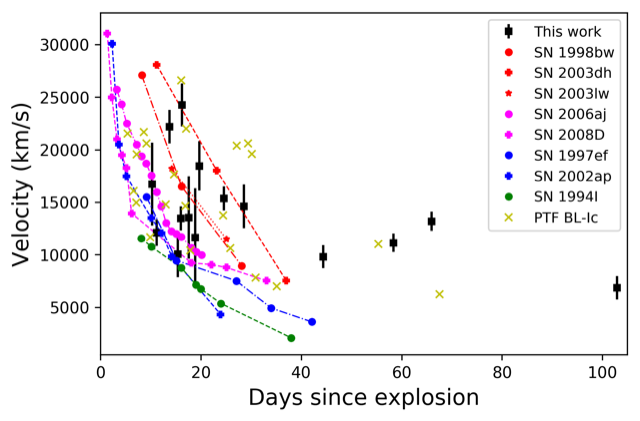
Figure 2: SN velocities measured from the Fe II 5169$\rm\AA$ line as a function of the spectroscopic phase for each supernova in our sample (black points) plotted along with the measured velocities of SNe Ic-BL from the literature and from PTF (Taddia et al., 2018). The velocities we measure here are broadly consistent with both the literature and PTF sample.

7.2 Comparing color-color predictions to observations

Optical-NIR colors are a useful diagnostic to determine whether SNe Ic-BL could be potential sites of r-process production. The high opacity of r-process elements causes emission from the enriched regions to shift to redder wavelengths.

In Figure 3, we plot colors with respect to the $r-$band as $r-X$ ($X=J,H,K_{s}$) for r-process enriched models corresponding to the following parameters: “high mass, high velocity”: $M_{\rm ej}$$=7.93\rm\,M_{\odot}$, $\beta_{\rm ej}$$=0.25c$, $M_{\rm 56}$$=0.85\,\rm M_{\odot}$ (solid line), “medium mass, medium velocity”: $M_{\rm ej}$$=2.62\,\rm M_{\odot}$, $\beta_{\rm ej}$$=0.038c$, $M_{\rm 56}$$=0.39\rm\,M_{\odot}$ (dotted line), and “low mass, low velocity”: $M_{\rm ej}$$=1.00\rm\,M_{\odot}$, $\beta_{\rm ej}$$=0.033c$, $M_{\rm 56}$$=0.07\rm\,M_{\odot}$ (dashed line). This set of models illustrates how different combinations of assumed parameters affect the color curves. These specific model grids were used to fit the light curves of three objects in our sample and represent the broad range of explosion parameters derived for our SNe.

We use these color evolution predictions from the models to compare against the optical-NIR colors of our SNe. Our $r-X$ color measurements rely on two different methods: if there is an optical data point within three days of the NIR data point, we compute the color difference directly (filled circles); otherwise, we estimate the color by subtracting the NIR photometry from a scaled and shifted optical template (open circles). We construct this template from the light curve of SN 2020bvc, one of the SNe with the most well-sampled light curves, and then compute the shift and scale factors needed for the template to fit the data. For the cases in which the optical model does not fit the optical light curve perfectly, there can be a systematic offset between the open and closed circles. For example, the estimated $r-K_{s}$ color of SN 2019xcc (Figure 3, bottom panel) is $>1$ mag, but this is likely attributed to the fact that there is no concurrent optical photometry along with the $Ks-$band data point, and the optical light curve fades much faster than that of SN 2020bvc.

The predicted $r-J$ colors for r-process collapsar light-curve models range from $r-J\sim-$0.5 mag to $r-J\sim$1.5 mag. In the lefthand-side panels of Figure 3, we fix the mixing fraction to a moderate value of $M_{r\mathrm{p}}$$=0.3$ and vary the amount of r-process ejecta mass. On the righthand-side panels, we fix the r-process ejecta mass to 0.01M_⊙ and vary the mixing fraction. The amount of reddening in the model light curves is more strongly affected by the amount of mixing assumed; even for the lowest value of $M_{r\mathrm{p}}$, we find prolific reddening predictions for high mixing fractions relative to models with moderate mixing fractions and high r-process yield.

However, r-process enrichment is not the only factor affecting colors; unenriched SN models also have a range of colors, depending on their masses, velocities, and nickel production. Even amongst different models with identical r-process composition, color evolution can be sensitive to the explosion properties assumed. Here, the “high mass, high velocity” model set also shows the most dramatic reddening predictions for models that have extreme mixing; in general, higher mass models tend to show larger $r-X$ colors.

Late-time interaction with the circumstellar medium is also known to affect the color evolution of SNe (Ben-Ami et al., 2014; Kuncarayakti et al., 2022). While this is a rare phenomenon in SNe Ic-BL, SN 2022xxf showed evidence for a clear double-peaked light curve and narrow emission-line profiles in the later-phase spectra characteristic of interaction with a H/He-poor CSM (Kuncarayakti et al., 2023). SN 2022xxf also exhibited a dramatic red-to-blue color evolution as a result of interaction. We do not observe any of the above evidences for CSM interaction in our Ic-BL SNe, and therefore consider it unlikely that interaction could account for bluer colors at later times.

When comparing our color measurements against r-process models, we find that several of our objects show colors similar to the r-process models with minimal mixing. However, after 50 days post-peak, our detections and upper limits altogether strongly suggest that our SNe are brighter in the optical compared to the NIR. In particular, as many of our SNe are detected in the $J-$band over a wide range of phases, we can constrain the $r-J$ color to $<\,-0.5$ after 50 days post-peak. On the other hand, only one object shows $r-J$/$H$/$K_{s}$ colors $\sim$ 0.5 mag: SN 2007I. In particular, SN 2007I exhibits an increase in its $r-J$ color until about 60 days.

While these empirical color comparisons can be useful for identifying any obvious reddening signature that could be a smoking gun for r-process enrichment, more detailed fitting is required to establish whether or not these SNe are r-process enriched. Hence, in the next section, we describe our detailed model fitting aimed at determining whether there is room for an r-process contribution to their light curves.

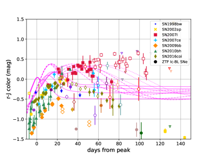
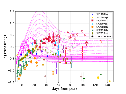
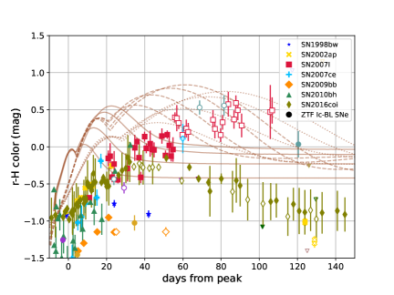
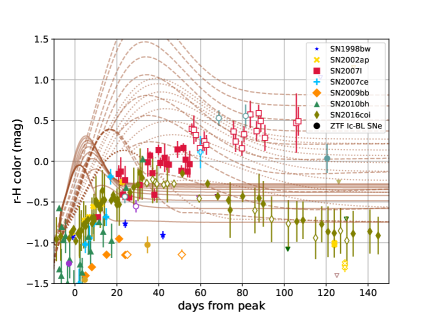
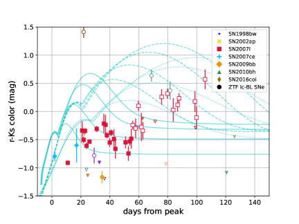
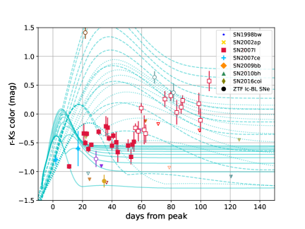
Figure 3: $r-J$, $r-H$, and $r-K_{s}$ color evolution plots for the r-process enriched models for a representative set of model parameters, compared to color measurements for the SNe in our sample. Each model is shown in a separate linestyle: “solid”: $M_{\rm ej}$$=7.93\rm M_{\odot}$, $\beta_{\rm ej}$$=0.25c$, $M_{\rm 56}$$=0.85\rm M_{\odot}$, “dotted”: $M_{\rm ej}$$=2.62\rm M_{\odot}$, $\beta_{\rm ej}$$=0.038c$, $M_{\rm 56}$$=0.39\rm M_{\odot}$, and “dashed”: $M_{\rm ej}$$=1.00\rm M_{\odot}$, $\beta_{\rm ej}$$=0.033c$, $M_{\rm 56}$$=0.07\rm M_{\odot}$. When possible, the $r-X$ color of observed SNe was estimated using either concurrent $r-$band photometry or the closest optical photometry within 3 days of a given NIR datapoint (filled markers). Otherwise, the $r-$band magnitude is extrapolated from a stretched and scaled light curve of SN 2020bvc (unfilled markers). Left: Fixing the mixing fraction to a moderate value of 0.3, we vary r-process ejecta masses [0.01, 0.03, 0.08, 0.13] M_⊙. Right: Fixing the r-process mass to a conservative value of 0.01 M_⊙, we vary the mixing coordinate from 0.1 to 0.9. In general, the objects in our sample appear to have bluer colors relative to the models (with the exception of SN 2007I).

8 Results of light curve Model Fitting

To quantitatively determine whether r-process contribution is required to explain the light curves of SNe Ic-BL, we perform nested sampling fits over multi-dimensional parameter space spanned by the r-process enriched models. However, in order to perform the fitting, we need a distribution over functions with a continuous domain. Since these r-process models are discretely parameterized, we invoke gaussian process regression (GPR) to predict light curves from the training set (which are the r-process enriched models, in this case) for each linear combination over the continuous ranges of parameters.

We first considered the full grid of r-process enriched models from Barnes & Metzger (2022). For objects for which it was possible to estimate the total ejecta mass and kinetic energy, we select grids where the parameters fall within the following bounds: $M_{\rm ej}{}\in(M_{\rm ej,0}-3\sigma,M_{\rm ej,0}+3\sigma)$, $\beta_{\rm ej}{}\in(\beta_{\rm ej,0}-3\sigma,\beta_{\rm ej,0}+3\sigma)$, and $M_{56}\in(M_{56}-3\sigma,M_{56}+10\sigma)$, where $M_{\rm ej,0}$, $\beta_{\rm ej,0}$, and $M_{56}$ are the independently derived explosion properties for the supernovae (see Table 4). We changed the upper bound on $M_{\rm ej}$ ($\beta_{\rm ej}$) to $M_{\rm ej,0}+10\sigma$ ($\beta_{\rm ej,0}+10\sigma$) for those SNe for which only a lower limit on those quantities was derived. We use the entire range of parameters in the grid for $M_{r\mathrm{p}}$ and $M_{r\mathrm{p}}$.

We then perform singular value decomposition on each light curve in the model grid tailored to each supernova and interpolate between model parameters using scikit-learn’s GPR package, sampling between $-5$ and 200 days relative to the supernova peak in a similar fashion to Coughlin et al. (2019) and Pang et al. (2022). We allow GPR to interpolate the range of r-process ejecta masses and mixing fractions between $M_{r\mathrm{p}}$$=$ 0.01 M_⊙, $M_{r\mathrm{p}}$$=$ 0.1 (which are technically the lowest values in the r-process enriched grid) and $M_{r\mathrm{p}}$$=0.00$, $M_{r\mathrm{p}}$$=0.0$, though we do not allow it to exceed the maximum values for these quantities (i.e. $M_{r\mathrm{p}}$$\leq$ 0.15 M_⊙ and $M_{r\mathrm{p}}$$\leq$ 0.9). We limit interpolation of the remaining explosion parameters within the maximum and minimum bounds of the original grid. For a given set of explosion parameters ($M_{\rm ej}$, $\beta_{\rm ej}$, $M_{\rm 56}$), each grid also contains an r-process-free model.

We compute a likelihood function based on the interpolated light curve models and our multi-band ZTF forced photometry, follow-up photometry, and WIRC photometry. Since the errors from GPR are small (i.e. they well-approximate the original model grid), we assume a systematic fitting uncertainty of 0.5 mag in the NIR bands and a fitting uncertainty of 1.0 mag in the optical. We converged upon a 1.0 mag systematic uncertainty in the optical after evaluating how different assumed errors affect the fit quality. The difference in the systematic errors is motivated by the fact that the NIR bands, rather than the optical bands, are a stronger determinant of whether there is evidence for r-process production. Furthermore, these assumptions on the systematic error compensate for the finer sampling in the optical bands relative to the NIR. In the likelihood calculation, we also impose a condition that rejects samples with a linear least squares fitting error worse than 1.0 mag. For the r-process enriched model fits, our prior also restricts the inference of parameters within the ranges of the grid (0.0 $\leq\rm x_{\rm mix}\leq$ 0.90; 0.0 M${}_{\odot}\,\leq\rm M_{r\mathrm{p}}\leq\,0.15\,\rm M_{\odot}$) and within physical constraints (i.e. $M_{r\mathrm{p}}$$<$ $M_{r\mathrm{p}}$($M_{\rm ej}$ - $M_{\rm 56}$)). We impose this upper limit on M_rp to satisfy the requirement that the r-process enriched core also contains ${}^{56}\text{Ni}$ (see Figure 8 of Barnes & Metzger 2022). Finally, we employ PyMultinest’s (Buchner et al., 2014) nested sampling algorithm to maximize the likelihood and converge on the best fit parameters and their uncertainties.

Most of the SNe in our sample show no compelling evidence for r-process production. In our model fits, the general trend we observe is that the best fit consistently under-predicts the peak of the optical light curve, while performing better at predicting the NIR flux. In some cases, the under-prediction is egregious, while in other cases it is more modest. In general under-prediction indicates that the optical-NIR color of the SN is actually bluer than predicted by the models, providing stronger evidence towards favoring r-process-free models over the enriched models. As mentioned earlier, as M_rp increases, the NIR light curve gets brighter; as $M_{r\mathrm{p}}$ increases, the optical light curve peak diminishes and the optical flux is suppressed more at later times.

To quantitatively assess the fit quality, we compute $\chi^{2}$ values between the best-fit model and the data points. We adopt the convention that if $\chi^{2}>\chi^{2}_{crit}$ (at the $>5$% level), we can reject our hypothesis that these SNe are well-described by the best-fit r-process enriched model. Therefore, given that our fits have 4 degrees of freedom, a $\chi^{2}>9.49$ is indicative that the r-process enriched models are poor fits to the data. Applying this criteria suggests that SN 2018gep, SN 2019xcc and SN 2020rph are very unlikely to harbor r-process material in their ejecta.

Similarly, we select the subset of objects for which $\chi^{2}<\chi^{2}_{crit}$ for a p-value of 0.90 ($\chi^{2}_{crit}=1.06$, for 4 degrees of freedom). Based on their $\chi^{2}$ values, SN 1998bw, SN 2007ce, SN 2018kva, SN 2019gwc, SN 2020lao, SN 2020tkx, SN 2021xv and SN 2021bmf show the most convincing fits to the r-process enriched models. Upon visual inspection of the remainder of the light curve fits, we find that none of the other objects are well-described by the r-process model predictions. We display the corner plots showing the posterior probability distributions on the derived parameters in Fig. 4 for the objects passing our $\chi^{2}$ cut, along with the best-fit light curves in Fig. 5.

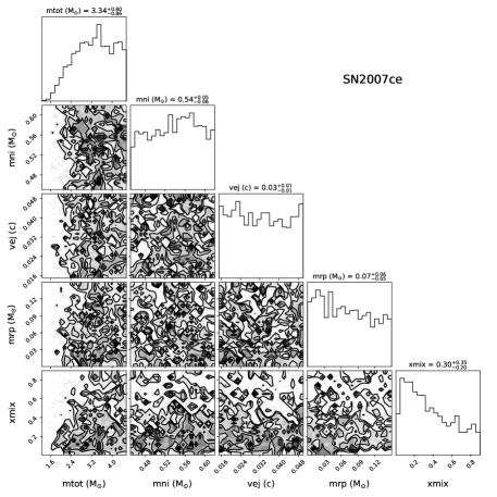
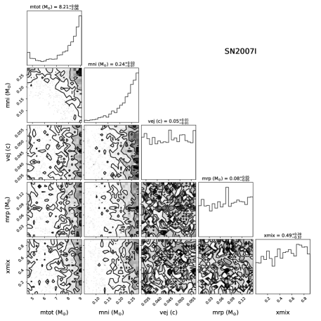
Figure 4: Corner plots showing the posterior probability distributions for each of the parameters in the r-process enriched models for the subset of objects satisfying our $\chi^{2}$ cut, ordered by the amount of r-process mass inferred. The posterior probability plots are more well-constrained for the objects with low inferred $M_{r\mathrm{p}}$; in the remaining cases, the posterior distributions are poorly constrained. $M_{\rm ej}$ and $\beta_{\rm ej}$ inferred here are generally in agreement with HAFFET, but discrepancies exist in the amount of nickel mass inferred.

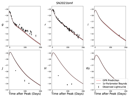
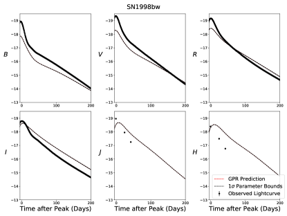
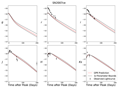
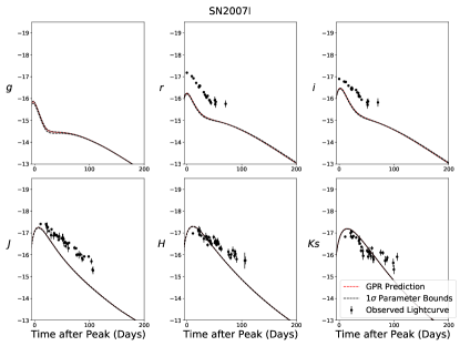
Figure 5: Plots of light curve models from Barnes & Metzger (2022) with best-fit parameters (red dotted line) and corresponding 1$\sigma$ uncertainties (black) with photometric data overplotted, for both ZTF candidates and candidates from the literature shown in Figure 4 which pass our $\chi^{2}$ cut, ordered by inferred $M_{r\mathrm{p}}$. The objects whose optical and NIR photometry are both well-described by the models are consistent with $M_{r\mathrm{p}}$$\lesssim 0.01\rm M_{\odot}$. The remaining objects do not show convincing fits to the r-process enriched models.

8.1 r-process Candidate ZTF SNe

Only two of the SNe in this subset have well-constrained parameters derived from the corner plots: SN 2020lao and SN 2021xv. The remainder of the objects have nearly flat posteriors on $M_{\rm 56}$ and $\beta_{\rm ej}$. For SN 2019gwc the peaks of the posterior probability distributions for both M_rp and $M_{r\mathrm{p}}$ are consistent with zero. This is supported by the fact that while both the $r-$band and $i-$band light curves are slightly under-predicted by the models, the $J-$band flux is also over-predicted; the observed colors are bluer than a best-fit model with negligible r-process. SN 2020lao and SN 2021xv, in turn, have a best fit value of M${}_{r\mathrm{p}}=0.01\,\rm M_{\odot}$ and $M_{r\mathrm{p}}$ $<\,0.1$. In the case of SN 2020lao, the optical flux is under-predicted by the models, and there are no NIR detections. On the other hand, for SN 2021xv, the optical models provide a decent fit to the optical data, but the NIR flux is still slightly over-predicted by the models.

SN 2018kva, SN 2019moc, SN 2020tkx and SN 2021bmf show posterior support for higher r-process enrichment. SN 2020tkx and SN 2018kva have inferred values of $M_{r\mathrm{p}}$$\sim 0.03\,\rm M_{\odot}$ and $M_{r\mathrm{p}}$$\lesssim 0.1$. For these two objects, the model under-predicts the peak of the optical light curve, though for SN 2018kva the $J-$band models fit the corresponding photometry. SN 2020tkx has two NIR detections in each of $J$, $H$, and $K_{s}$ filters which are well below the NIR model prediction, demonstrating that its light curve is inconsistent with the r-process enriched model. Finally, SN 2019moc and SN 2021bmf have parameter fits consistent with M${}_{r\mathrm{p}}\gtrsim 0.03$ and $M_{r\mathrm{p}}$$\gtrsim 0.1$. Similar to other cases, the best fit model for SN 2019moc under-predicts its optical light curve. While the model is consistent with the $K_{s}-$band upper limit, it still over-predicts the $J-$band flux. SN 2021bmf has one of the best-sampled optical light curves in our sample, and the model provides a beautiful fit to the optical bands. However, the NIR photometry is still vastly over-predicted by the same model.

8.2 r-process Candidate Literature SNe

Similarly, the two objects with $\chi^{2}$ fits that pass our criteria are SN 1998bw and SN 2007ce. In this category we also include SN 2007I because it shows more significant photometric reddening relative to the other objects in the sample, even though it does not pass our nominal cuts.

The corner plots for these three objects show posterior distributions that are not well-constrained. However, all three objects have high predicted values for both $M_{r\mathrm{p}}$ as well as $M_{r\mathrm{p}}$. The light curve fits show the same phenomenon that we identify for the ZTF SN light curve fits: the peak of the optical light curve is under-predicted, while the NIR data shows better agreement with the models. In the case of SN 1998bw, the low $\chi^{2}$ is likely attributed to the fact that the optical data are extremely well-sampled, and the model provides a decent fit to its late-time light curve (in the $B$, $V$, and $R-$ bands), but the same model does not describe the decay in the NIR flux accurately. The best-fit model for SN 2007ce matches the NIR bands but again under-predicts the optical. For SN 2007I, the $riJ$-band fluxes are wholly underestimated, and in the $HK$-bands, the light curve appears to be declining much slower than predicted by the models.

As emphasized by Barnes & Metzger (2022), color evolution can be a more powerful metric in comparison to absolute magnitude comparisons between the model light curves and data in determining whether a SN Ic-BL harbors r-process material. We thus plot color evolution ($r-J/H/K_{s}$) as a function of time for our two reddest objects, SN 2007I and SN 2007ce. In Figure 6 we show their photometric colors along with their best fit r-process-free and r-process enriched models. In the shaded regions we include the $\pm 1\sigma$ uncertainty on the model parameters from our fits. SN 2007ce’s colors appear too blue in comparison with its best-fit r-process model. We note that the color measurements for this object are secure because of several contemporaneous optical-NIR epochs. Given that it only attains a maximum $r-X$ color of $\sim$0.1 mag 50 days post-peak, we conclude that SN 2007ce is most likely not an r-process collapsar. SN 2007I is completely inconsistent with the color evolution of its best-fit r-process model, even within the parameter uncertainties. However, one challenge arises from the fact that in the late-time ($\gtrsim$50 days post-peak) SN 2007I lacks any optical photometry. Based on our extrapolation of the $r-$band light curve of SN 2007I we see evidence for further reddening which starts to become consistent with the r-process enriched model predictions in the late-times. Thus, we are unable to rule out the possibility of r-process production in SN 2007I based on the r-process fits and the color evolution comparison alone.

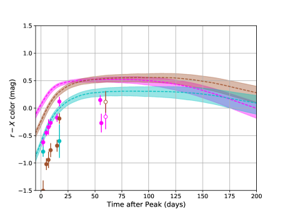
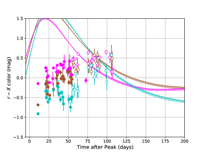
Figure 6: Color evolution as a function of time for both SN 2007ce (left) and SN 2007I (right). Similar to Figure 3, the filled circles with errobars represent the $r-J/H/K_{s}$ color estimated directly from the data, while the unfilled circles correspond to a stretched and scaled $r-$band model of SN 2020bvc used as a proxy to estimate the color at each NIR photometric epoch, in the absence of $r-$band photometry. The dashed line represents the color evolution of the best-fit r-process enriched model, and the shaded regions encompass the $\pm 1\sigma$ uncertainty on the model parameters from our fits. Using the same convention as in Figure 3, magenta is $r-J$, brown is $r-H$ and cyan is $r-K_{s}$. As shown here, the color evolution of both SN 2007I and SN 2007ce appear to be inconsistent with their best-fitting r-process enriched model colors and associated 1$\sigma$ uncertainties.

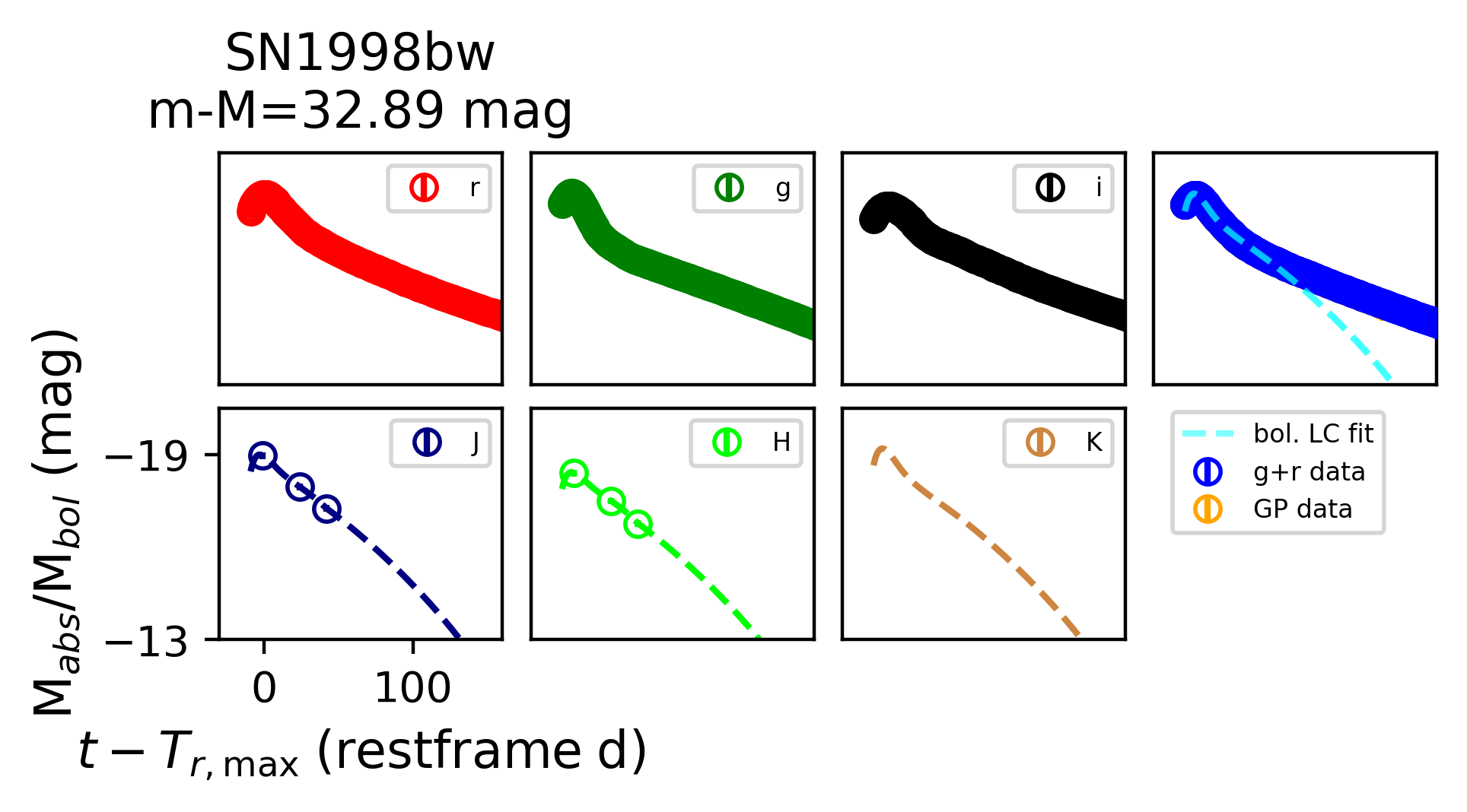
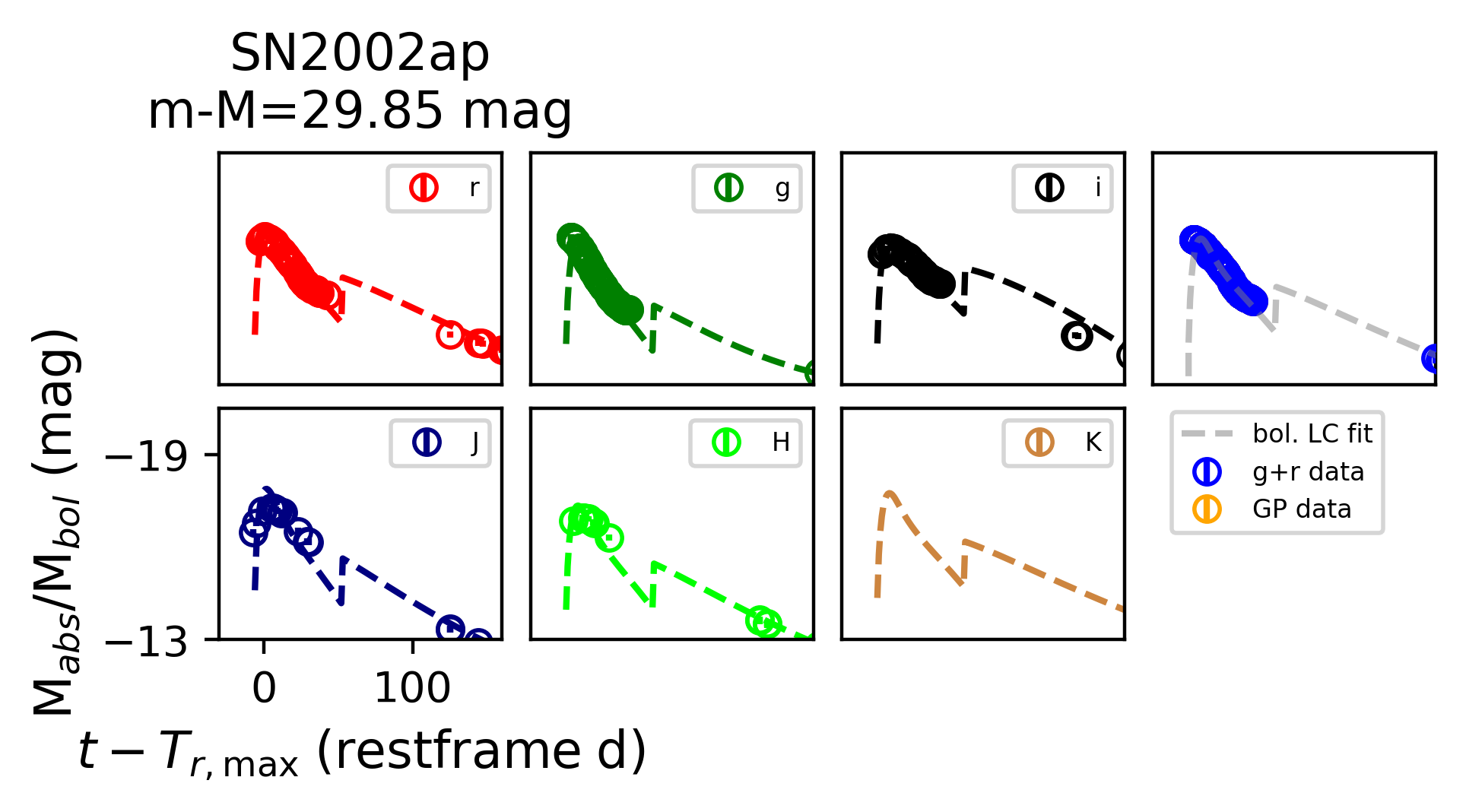
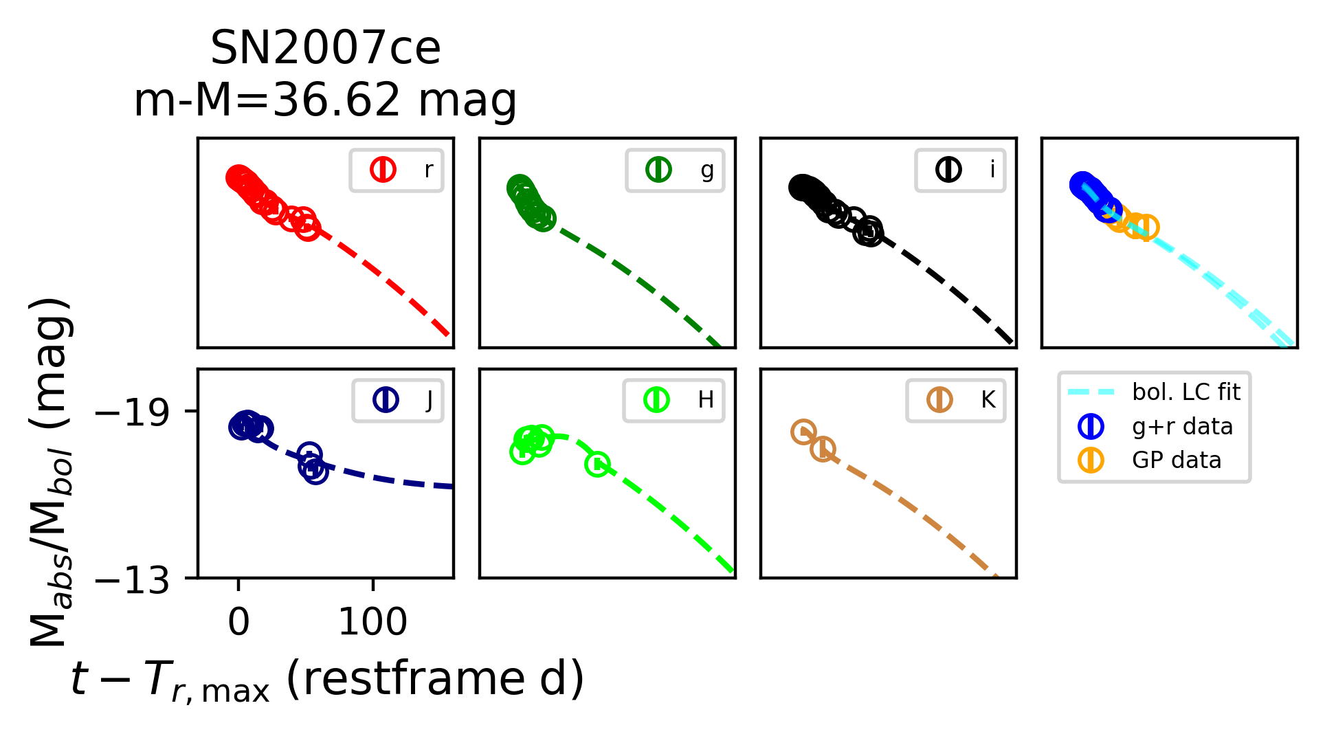
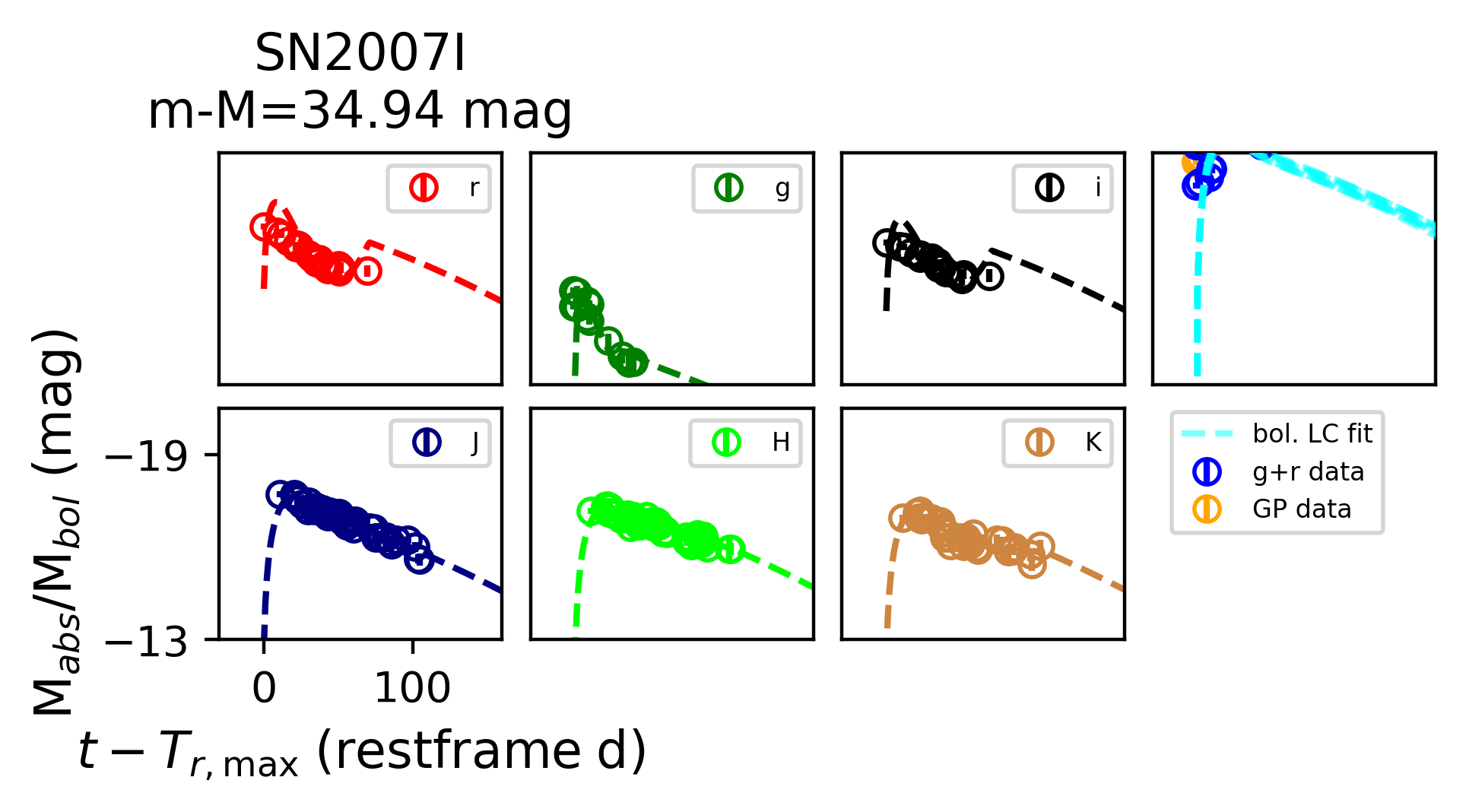
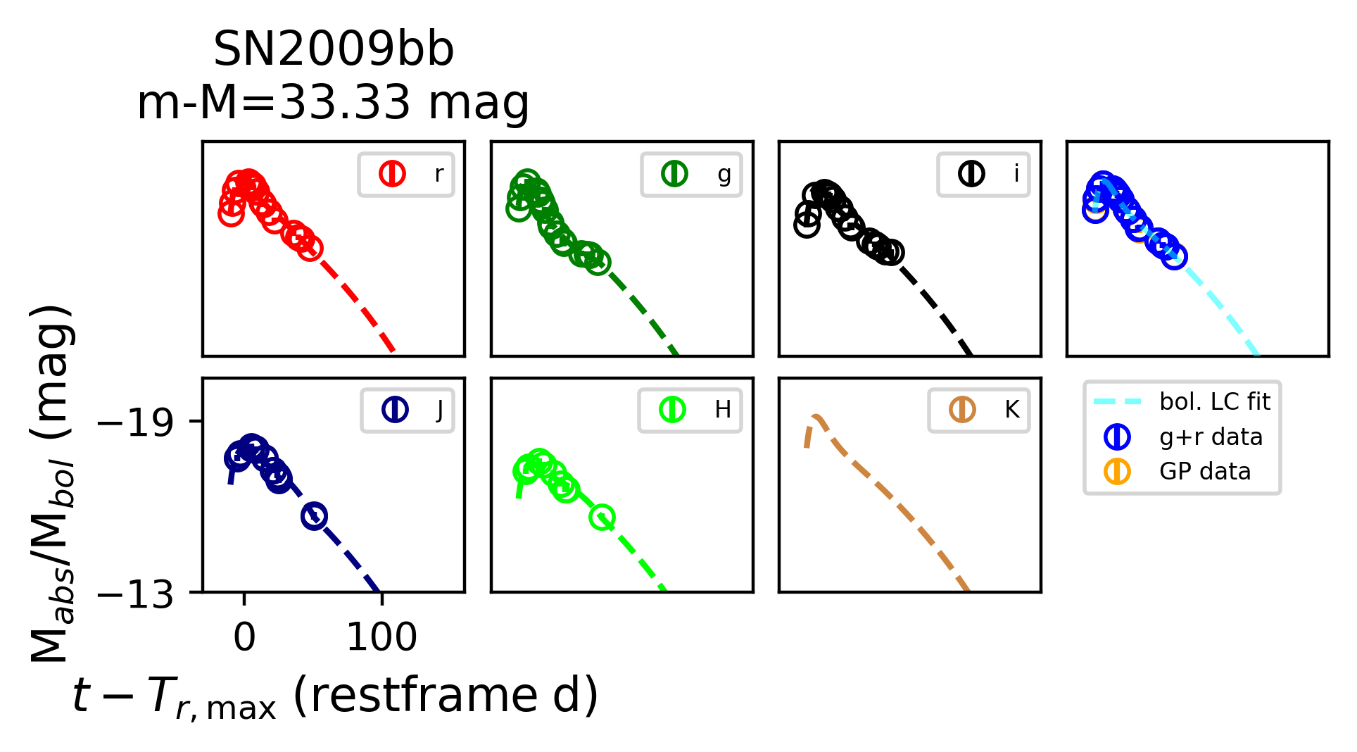
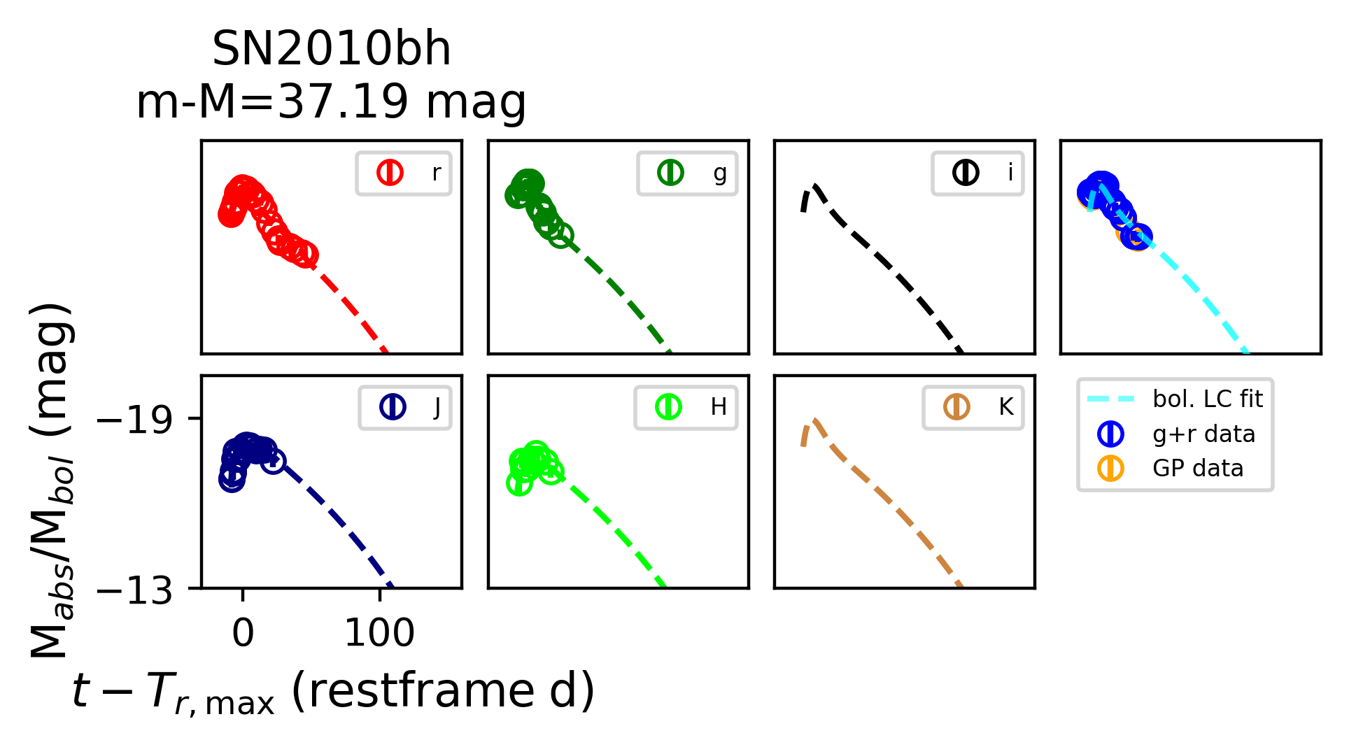
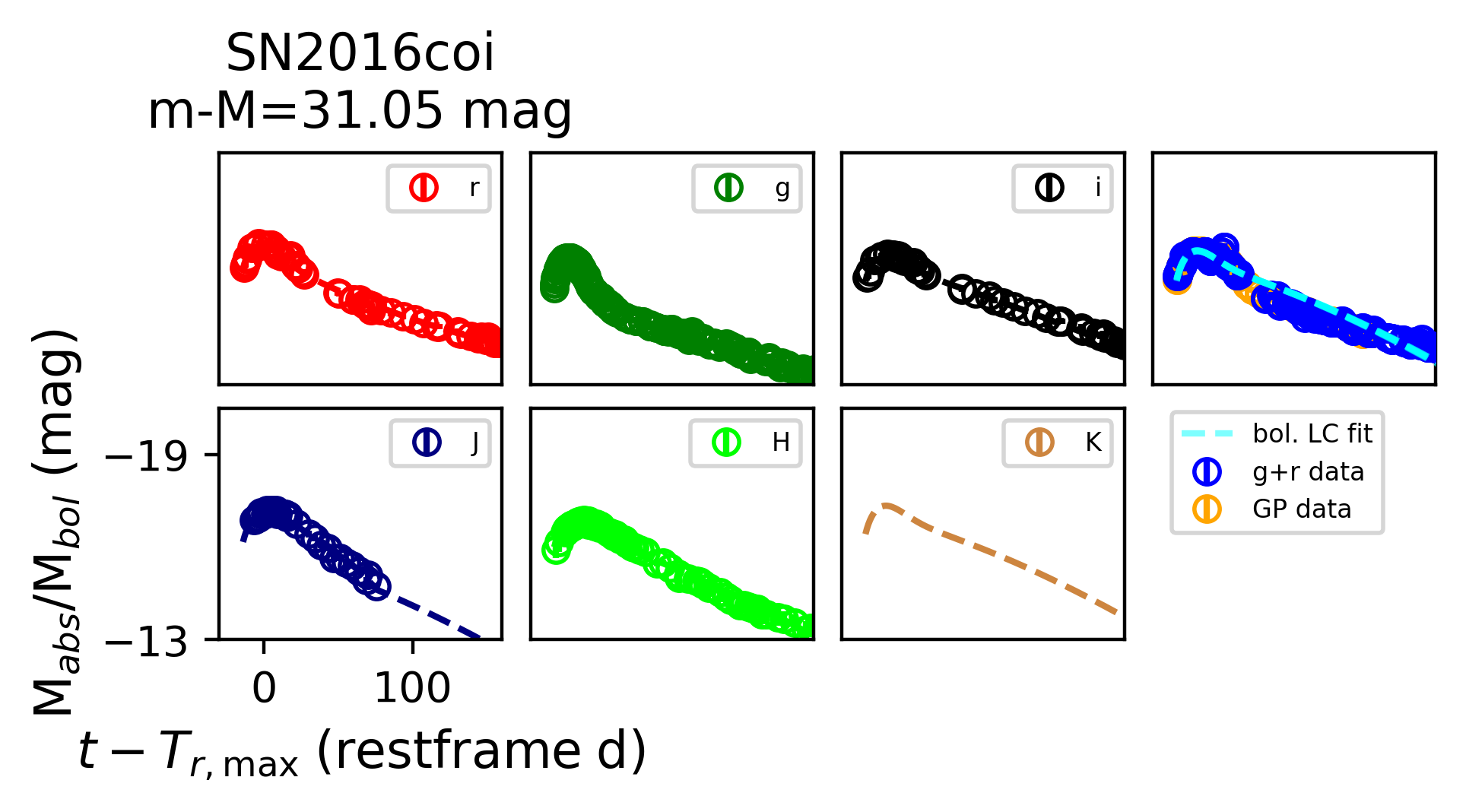
Figure 7: Light curve fits to the literature supernova events from HAFFET. The dashed cyan line is the best fit bolometric light curve, while the remaining dashed lines show the fits to each of the broadband light curves. Broadband light curves are calculated by fitting bolometric corrections in each band, and using these corrections to rescale the Arnett fitted bolometric light curves. The circles are the photometry for each object in $griJHK_{s}$ bands. In the bolometric light curve plot, the points correspond to bolometric luminosity estimated from both $g-$ and $r-$ bands, or from a single band, and using GPR to estimate the flux in the other band. For SNe with photometry in the Johnson filter system, we convert the photometry to SDSS assuming photometric conversions from Jordi et al. (2006). We find that the HAFFET models are good fits to the photometric data from our sample.

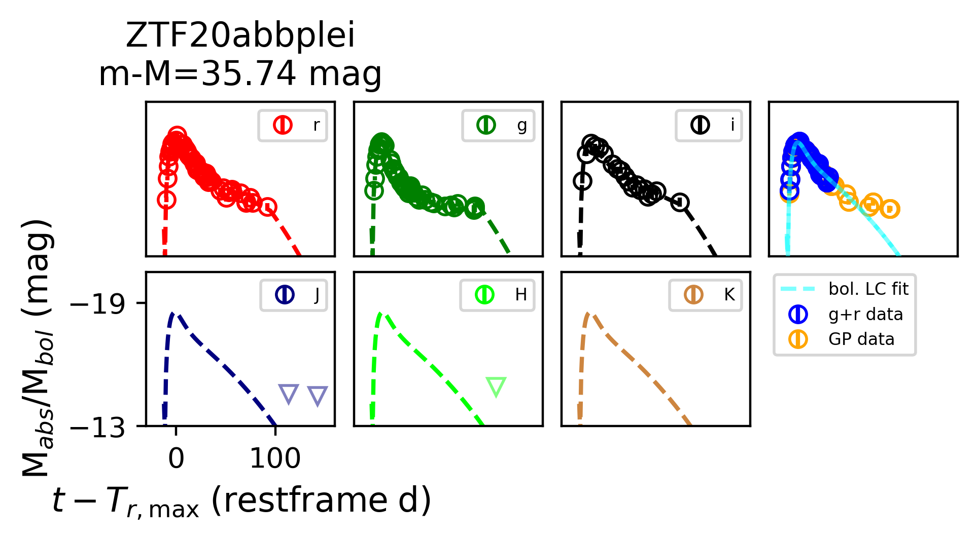
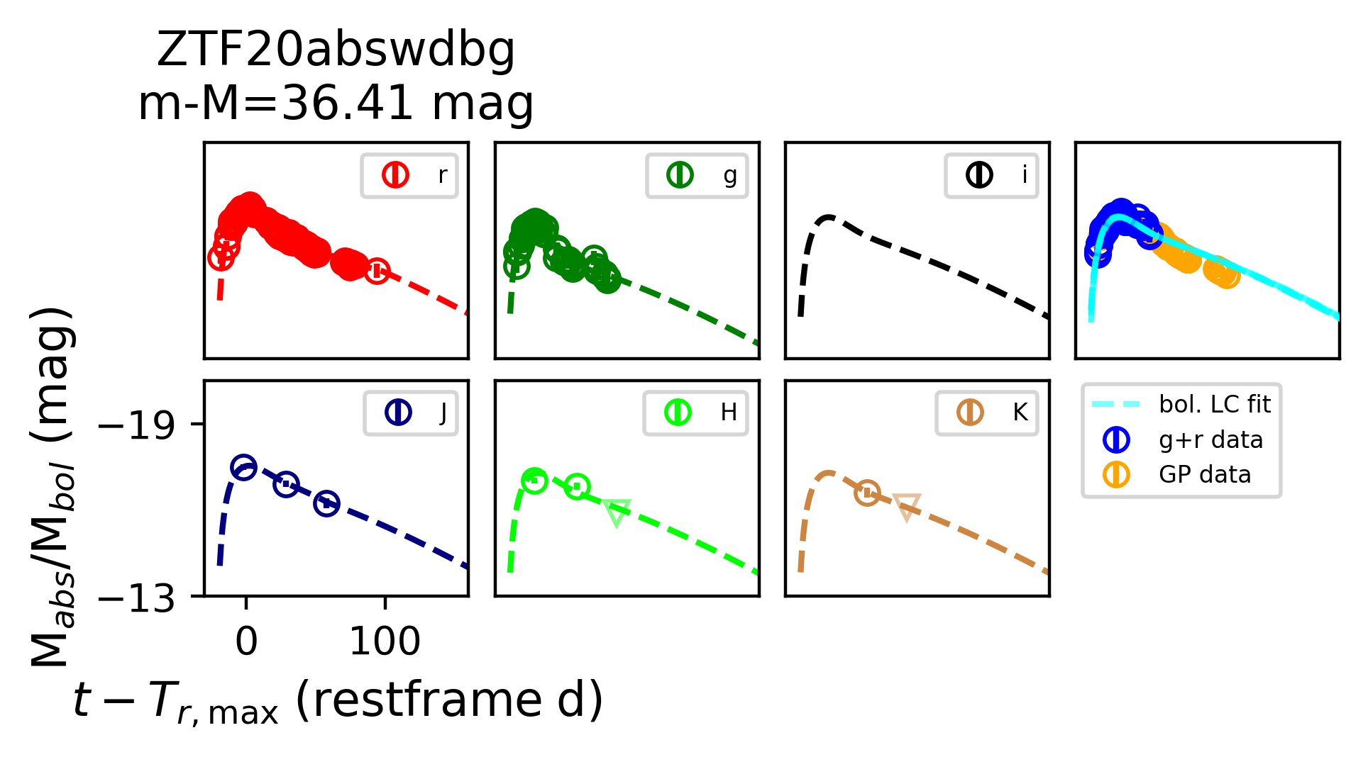
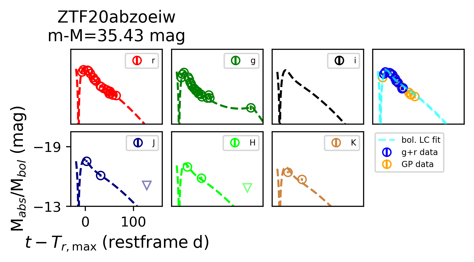
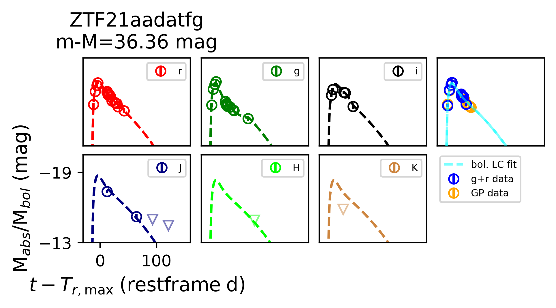
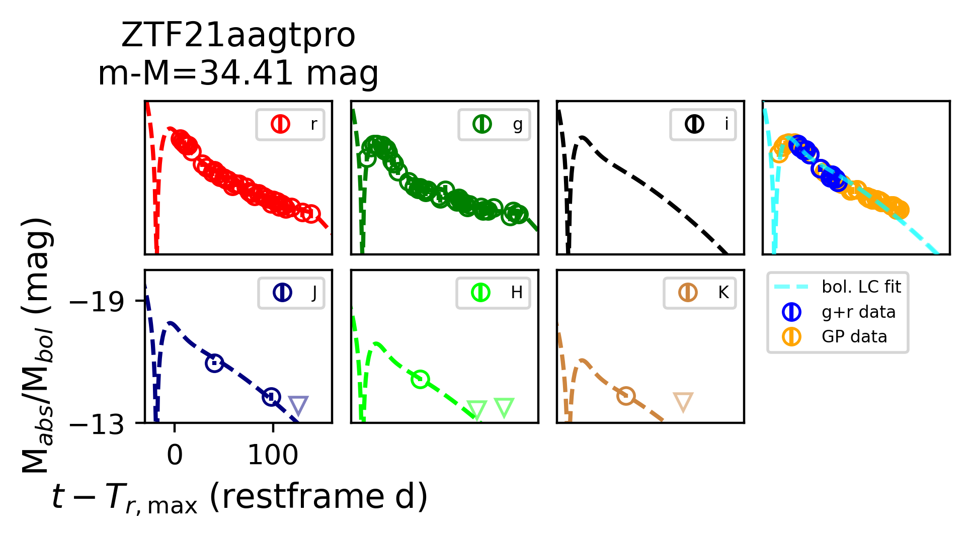
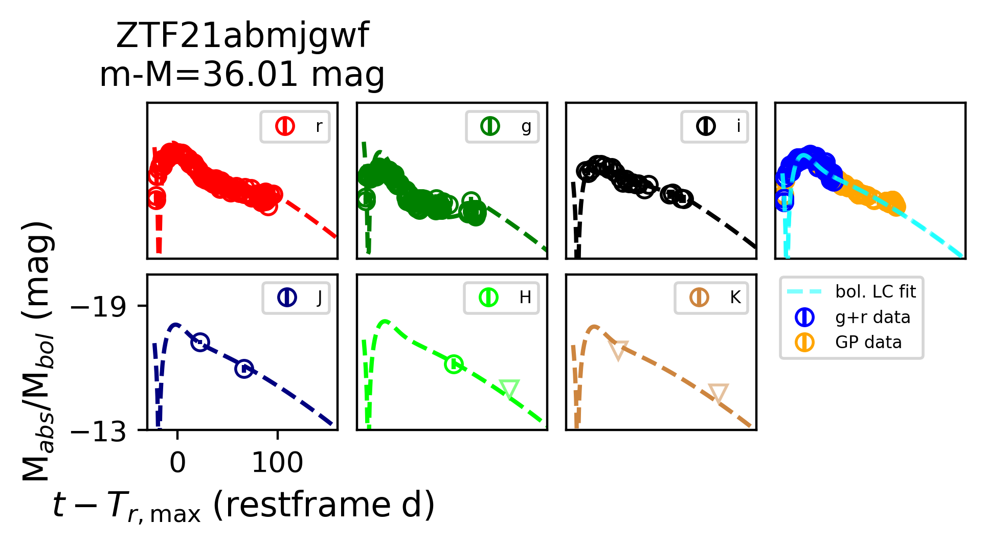
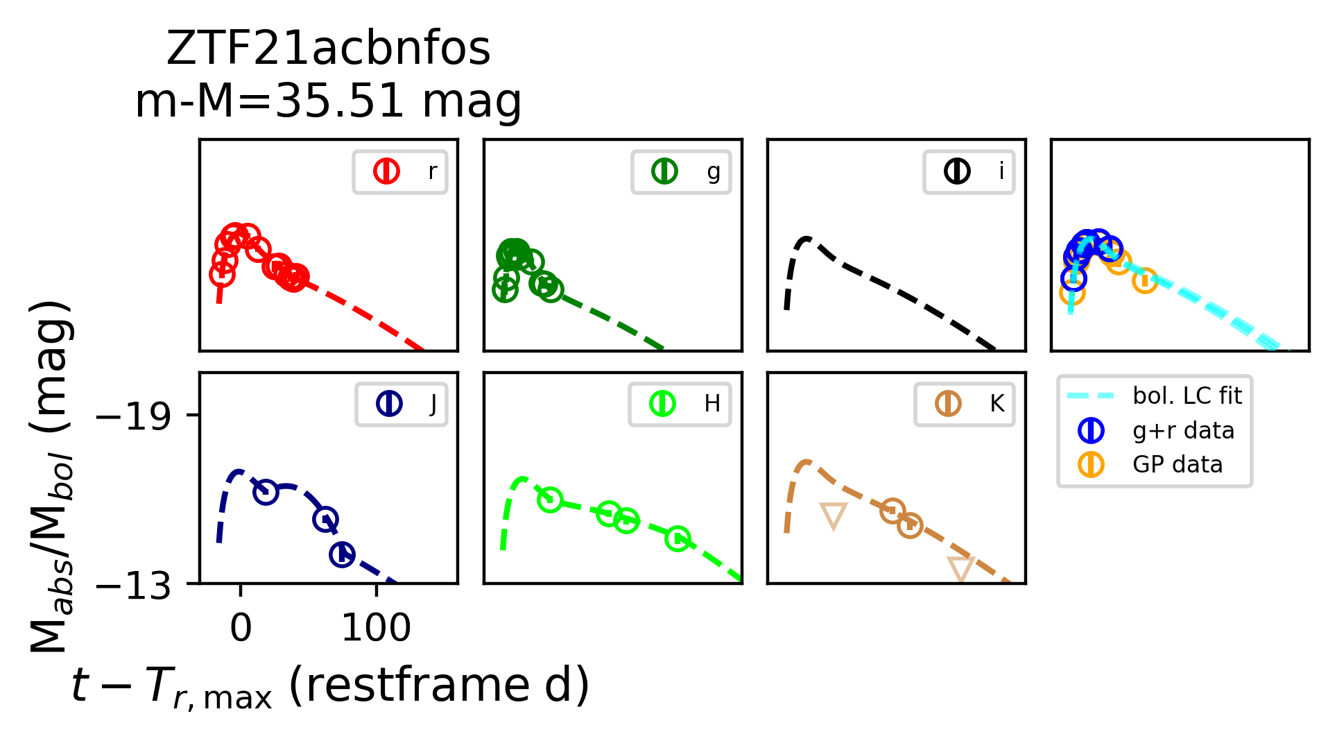
Figure 8: Light curve fits to ZTF SNe from HAFFET, similar to Fig. 7.

8.3 Independent Arnett Fits

To supplement our fits to r-process enriched models we use HAFFET to construct a bolometric light curve from our optical data and fit to the standard Arnett model (as described in more detail in Sec. 7). We then calculate broadband light curve models by fitting bolometric corrections in each band, and using these corrections to rescale the Arnett fitted bolometric light curve models. Our fits are shown in Figures 7 and 8.

In order to compare the two models, we compute $\chi^{2}$ for each of the broadband light curves in the same way as we did using the r-process-enriched models. We find that all of the objects, except for SN 2021xv, have lower $\chi^{2}$ values with the HAFFET fits compared to the r-process model fits, insinuating that the r-process-free models are a better descriptor of these SN light curves. Aside from 3 objects, all other objects pass our criteria of $\chi^{2}<1.06$ (i.e. well-described by the r-process-free models) and none of them have $\chi^{2}>9.49$ (i.e. poorly described by the r-process-free models). Upon visual inspection, we find convincing fits to both the early optical light curves and the NIR light curves of these objects for the r-process-free models. In the case of SN 2021xv, we note that the r-process parameter estimation favors little to no r-process mass and mixing, and the r-process-enriched models overestimate the NIR flux. Thus we consider SN 2021xv to still be consistent with an r-process-free scenario.

Furthermore, we derive blackbody effective temperatures for the closest epoch to 30 days post-peak where both optical and NIR photometry are available. The effective temperatures range from $4000-15000$ K; the SED colors are well-described by a single-component blackbody at this phase. Based on the quality of our Arnett fits, and the fact that the SED for these SNe in the photospheric phase is well-described by a blackbody, we conclude that no r-process contribution is needed to explain the color evolution of the objects in our sample, including SN 2007I.

Thus, we find no compelling evidence of r-process enrichment in any of the SNe in our sample.

9 Discussion and Outlook

From our systematic study in optical and NIR of the SNe Ic-BL associated with collapsars discovered by ZTF and reported in the literature, we do not find any evidence of r-process enrichment based on theoretical models which predict observable NIR excesses in the SN light curves. After constructing GPR models from the r-process-enriched model grid and performing fitting, the SNe that pass our nominal $\chi^{2}$ cuts still do not show convincing fits in both the optical and NIR to the r-process enriched broadband light curve predictions. On the other hand, for the r-process-free models, when computing broadband light curves from the bolometric corrections, we get compelling fits in both optical and NIR for each SN. Our single-component blackbody fits at $\sim$1 month after peak (see Table 4) further suggest that no additional r-process enrichment is required to explain the SN SED colors.

Our use of two models, one for r-process-free SNe and another for r-process enriched cases, complicates our efforts to derive global constraints on r-process production in SNe. To estimate the level of enrichment our analysis is sensitive to, we take the reddest object in our sample that is consistent with the r-process enriched models, and compare the color measurements with the predicted color evolution from the models. To derive these global constraints, we focus on SN 2007ce. Amongst our sample, SN 2007ce has the highest inferred r-process ejecta mass of 0.07M_⊙ while passing the $\chi^{2}$ cut (we ignore SN 1998bw, whose extremely well-sampled light curve could be influencing the final $\chi^{2}$ value). Though SN 2007I is redder than SN 2007ce, it shows color evolution that is completely inconsistent with the models (see Fig. 6) making it unsuitable for deriving r-process constraints. In Fig. 6 we display the predicted color evolution of the best fit model bounded by its 1$\sigma$ uncertainties on the parameters, where the lower bound corresponds to a model with $M_{r\mathrm{p}}$$=0.02\rm M_{\odot}$ and the upper bound corresponds to a model with $M_{r\mathrm{p}}$$=0.12\rm M_{\odot}$. SN 2007ce’s color measurements exhibit a similar shape to the model color evolution, but show a significant offset with bluer colors compared to the best-fit models. As shown in Figure 3, a model with a higher $M_{\rm ej}$ can yield a slightly bluer color evolution for the same r-process mass, so it is difficult to confidently exclude the possibility that $M_{r\mathrm{p}}$$=0.02\rm M_{\odot}$ (the lower bound on the parameter inference) was synthesized in SN 2007ce. In addition, relaxing the assumptions on the SED underlying the models could also alter the color evolution of the model. Thus, based on the the upper bound of these color curves, which corresponds to an r-process mass of 0.12M_⊙, we conservatively argue here that no more than 0.12M_⊙ of r-process material was generated in SN 2007ce (assuming $M_{r\mathrm{p}}$$=0.7$). Furthermore, since SN 2007ce has the highest inferred r-process mass amongst the objects passing our $\chi^{2}$ cut, we suggest that $M_{r\mathrm{p}}$$\lesssim 0.12\rm M_{\odot}$ represents a tentative global r-process constraint on all of the models in our sample, based on the observations. Future improvements in the models as well as more systematic observations will allow for tighter and more robust constraints on the r-process nucleosynthesis in SNe Ic-BL.

We also examine any other associated relativistic outflows to check whether that may introduce a bias. Only three objects in our full sample are counterparts to GRBs: GRB980425 (SN 1998bw), GRB100316D (SN 2010bh) and GRB190829A. Amongst these three, GRB980425 and GRB190829A are considered to be LLGRBs based on their peak $\gamma$-ray luminosities (Galama et al., 1998; Ho et al., 2020b; Dichiara et al., 2019). GRB100316D is a more energetic GRB, but its emission shows a soft spectral peak, similar to other X-ray flashers (Bufano et al., 2012). While none of the other objects in our sample have any coincident $\gamma$-ray emission, some have X-ray and radio detections and upper limits. SN 2018gep, the FBOT/SN Ic-BL, has both X-ray and radio detections that are consistent with the host galaxy emission (Ho et al., 2019). On the other hand, SN 2020bvc has mildly-relativistic X-ray and radio ejecta characteristic of LLGRBs (Ho et al., 2020a). Corsi et al. (2023) also obtained radio and X-ray follow-up for several ZTF SNe, a subset of which are part of the sample discussed in this work. In Table 1 we display radio observations with the Very Large Array (VLA) and X-ray observations with the Swift X-ray Telescope (XRT) for those SNe; the remainder of SNe which lack radio/X-ray coverage have dashes in those respective columns. Only two of the objects in the sample presented here (SN 2020tkx and SN 2021ywf) have a detected point-source-like radio counterpart, but their low velocities suggest that they are not the same as GRB-associated SNe (Corsi et al., 2023).

The fact that none of these SNe are linked to standard, classical long GRBs prevents us from exploring the proposed theoretical connection between the GRB energetics and r-process production. If the GRB jet energy, which scales with the mass accreted by the disk, correlates with the amount of r-process mass produced in the disk winds, then collapsars with no GRBs may not be able to produce detectable r-process signatures. Siegel et al. (2019) find that for black hole accretion rates between 0.003$-$1.0 M_⊙ s^-1 needed to power relativistic outflows, the disk winds are neutron-rich and can synthesize heavy and light r-process elements. The association of a GRB with a SN Ic-BL could point towards a central engine that harbors high enough accretion rates to potentially generate r-process elements. Barnes & Duffell (2023) also find that hydrodynamical mixing between the r-process enriched and r-process-free layers of collapsar increases with wind mass and duration, suggesting that SNe accompanying the longest duration long GRBs may be the most promising sites to search for obvious r-process signatures.

It is yet unclear to what extent the populations of SNe Ic-BL and long GRBs overlap (Woosley & Bloom, 2006; Bissaldi et al., 2007; Cano et al., 2017a; Barnes et al., 2018), as some long GRBs lack SNe (Fynbo et al., 2006; Della Valle et al., 2006; Tanga et al., 2018), and most Ic-BL SNe have no associated gamma-ray emission (Bianco et al., 2014; Corsi et al., 2023). Furthermore, LLGRBs, short-duration GRBs with collapsar progenitors (Ahumada et al., 2021) and long-duration GRBs from compact binaries (Rastinejad et al., 2022) present evidence towards a broad diversity in collapsar central engines, ranging from mildly relativistic to ultra-relativistic explosion energies. One possibility is that a subset of SNe Ic-BL could correspond to failed GRBs with low black hole accretion rates (MacFadyen & Woosley, 1999; Huang et al., 2002; Xu et al., 2023). Multi-wavelength observations of SN 2006aj suggest that another subset may be associated with a progenitor whose jet runs into a cocoon of extended stellar material (Nakar, 2015), even when an LLGRB is not detected, as in the case of SN 2017iuk (Izzo et al., 2019). Yet another subset could be off-axis GRBs.

This diversity of collapsar central engines and jet properties could lend itself naturally to a scenario where some collapsars are capable of producing r-process elements while others are not. However, given that only $\sim$half of the SNe in our sample have X-ray or radio observations, a more systematic NIR follow-up campaign with SNe Ic-BL associated with classical long GRBs, LLGRBs, X-ray/radio counterparts, and lacking any multi-wavelength counterparts is needed to investigate whether only those SNe that produce relativistic ejecta are able to create conditions conducive to r-process nucleosynthesis.

Another possibility we acknowledge is that collapsars could be a very low-yield source of r-process nucleosynthesis. The expected yields from the Siegel et al. 2019 and Barnes & Metzger 2022 models (0.01-0.1M_⊙) are mainly set by the joint constraints from the literature on r-process nucleosynthesis sites (see for e.g. Hotokezaka et al., 2018). However, the discovery of minuscule amounts of Sr and Ba in an extremely metal-poor star (Casey & Schlaufman, 2017) motivates the need for core-collapse supernovae with an extremely low yield of r-process material whose nucleosynthesis is consistent with the Solar r-process abundance pattern. Due to the limitations of these models and the dataset presented here, our study only searches for enrichment levels of $M_{r\mathrm{p}}$$\gtrsim 0.01\rm M_{\odot}$. Detailed analysis of the nebular-phase spectra of SNe Ic-BL would likely be required to probe such low levels of enhancement robustly.

Despite the fact that we find no evidence for r-process enrichment in the SNe Ic-BL in our sample, we must also acknowledge a number of caveats to this work.

First, we note that the r-process enriched and r-process-free models make different predictions about the relationship between nickel mass and SN luminosity. While the inferred central values from the GPR inference of both $\beta_{\rm ej}$ and $M_{\rm ej}$ based on the r-process grid are generally within the 1$\sigma$ errorbar of our explosion property estimates, the nickel mass inferred shows a larger deviation from the Arnett value. Arnett-like models are constructed such that the radioactive energy-generation rate crosses the bolometric light curve precisely at peak luminosity. The r-process enriched models, in which energy diffuses through a series of concentric shells, do not reproduce this behavior; they generally have $L_{\rm bol}(\rm tpk)<Q_{\rm dot}(\rm tpk)$. As a result, the amounts of nickel inferred by each model for a given luminosity are inconsistent, and the Arnett-like models do not match the Barnes & Metzger (2022) models when $M_{r\mathrm{p}}$ is set to zero (see Sec. 6 for other differences between the Barnes & Metzger (2022)-like models and the Arnett-like models). To compensate for these differences, we fit the r-process enriched models over a wide range of nickel masses.

Given the differences between the r-process enriched and r-process-free models we use, a more robust approach would be to conduct an apples-to-apples comparison between r-process-free and r-process enriched models from the same underlying grid. Initially, we performed fitting to both the r-process-free and r-process enriched models from (Barnes & Metzger, 2022), but found that the colors of the r-process-free models were consistently much redder than the observed colors of our objects at all epochs. To construct the r-process-free SED, Barnes & Metzger (2022) uses the light curve of SN 2007gr as it has well-sampled $B$- to $K$-band photometry up to late-times, but the detection of the CO molecule in its nebular phase NIR spectra may affect the $K-$band flux of the object (Hunter et al., 2009). Unfortunately, the semi-empirical approach to converting between bolometric and broadband light curves using HAFFET and the fact that the Arnett models do not allow us to define a spatial or velocity mixing coordinate renders the alternative possibility of enriching the HAFFET models with r-process material infeasible. Our inability to use r-process enriched and r-process-free models from the same grid makes our investigation to search for r-process production less robust. The authors are currently investigating whether varying additional parameters controlling the r-process-free SED may lead to better fits to the data. This will be discussed in a future work.

Furthermore, our understanding of the emission of r-process ejecta in the nebular phase is quite limited. The radiation from r-process-enriched ejecta layers has a strong impact on the predictions of late-time photometry for the r-process grid. Barnes & Metzger (2022) adopts a temperature of 2500 K for the r-process SED because a black-body at this temperature reproduces the optical and NIR photometric colors of the nebular-phase kilonova model spectrum of Hotokezaka et al. (2021). However, kilonova nebular-phase modeling is still a topic of active investigation. Future studies of kilonova nebulae, both observational and theoretical, may refine our understanding of nebular emission from pure r-process outflows. Furthermore, differences between kilonovae and r-process-enriched SN (e.g., in their densities or their compositions) may mean that nebular-phase emission from the former is not a perfect predictor of nebular-phase emission from the latter.

Finally, we acknowledge the limitations of the dataset we present here for testing whether collapsars synthesize r-process elements. Due to the nature of our classical observing runs with WIRC, our NIR light curves are very sparse, and in some cases our upper limits are too shallow to be constraining. In contrast, future wide field of view NIR facilities (i.e. WINTER, DREAMS, PRIME) will enable systematic follow-up of nearby SNe Ic-BL discovered by contemporaneous wide-field optical surveys (i.e. ZTF, Pan-STARRS, ATLAS, Vera Rubin Observatory, etc) as well as counterparts to nearby long GRBs to late-times. The James Webb Space Telescope will grant the unique ability to probe the mid-infrared wavelengths and acquire IR spectroscopy to search for further signatures of r-process production. Higher cadence NIR photometry and nebular spectroscopy to search for the r-process signatures from collapsars would substantiate the results of this paper as well as determine whether the presence of a relativistic jet in the explosion is required for heavy element production. The authors plan to investigate the relative contribution of collapsars, neutron star mergers, and neutron star–black hole mergers towards the r-process abundance in the Universe in a future work. The next generation of optical and IR telescopes will open new windows to discoveries providing valuable insights into the open questions about r-process nucleosynthesis from collapsars.

SN	$M_{\rm ej}$	$E_{\rm K}$	$M_{\rm Ni}$	E(B-V)host	$T_{\rm eff}$ [phase]	Ref.
	(M⊙)	(foe)	(M⊙)		(K [day])
1998bw	10	50	0.4	0.06*	5919 [24.5]	Clocchiatti et al. (2011); Nakamura et al. (2001)
2002ap	2.5-5	4-10	0.07 (0.02)	0.09	5126 [30.5]	Mazzali et al. (2002)
2007ce	2.90 (0.63)	1.85 (0.89)	0.48 (0.01)	0.00	6310 [18.5]	Modjaz et al. (2008)**
2007I	6.87 (0.80)	7.63 (1.99)	0.10 (0.00)	0.34	4064 [33.5]	Modjaz et al. (2008)**
2009bb	3.4 (0.4)	6.2 (0.8)	0.20 (0.02)	0.540	3584 [22.6]	Taddia et al. (2018)
2010bh	2.21 (0.10)	11.34 (0.52)	0.21 (0.03)	0.30	6102 [23.5]	Olivares E. et al. (2012)
2016coi	4-7	7-8	0.15	0.00	4727 [32.1]	Terreran et al. (2019)

Table 3: Explosion properties and inferred r-process ejecta masses and mixing fractions of low-redshift SNe with contemporaneous optical and NIR imaging from our literature search. Where available, we quote the 1$\sigma$ uncertainties on the parameters in brackets. For SN 1998bw and SN 2002ap, we quote the ranges of explosion parameters corresponding to the best-fitting light curve models. *Clocchiatti et al. (2011) already corrected for host extinction; we use the assumed host extinction to correct only the NIR photometry. **For SN 2007I and SN 2007ce, as explosion properties were not estimated in the literature, we conduct light curve analysis to derive the best fit properties as described in Sec. 7.

Table 4: Optical properties of the BL-Ic SNe in our sample.

SN	$t_{\rm peak}$	$M_{\rm peak,r}$	$t_{\rm expl}$	$M_{\rm Ni}$	$\tau_{m}$	$M_{\rm ej}$	$E_{\rm kin}$	$v_{\rm ph}$	$T_{\rm eff}$ [phase]
	(MJD)	(mag)	(day)	(M⊙)	(day)	(M⊙)	($10^{51}$erg)	(c)	(K [day])
2018jaw	58455.70	-18.63 (0.08)	-18.74 ${}_{-0.66}^{+0.66}$	0.33 ${}_{-0.02}^{+0.02}$	13.63 ${}_{-1.38}^{+1.10}$	$>$ 1.41 (0.33)	$>$ 0.40 (0.16)	0.022 (0.004)	–
2018kva	58487.05	-18.70 (0.02)	-15.81 ${}_{-0.60}^{+0.49}$	0.29 ${}_{-0.01}^{+0.01}$	12.13 ${}_{-0.87}^{+1.06}$	2.51 (0.39)	3.53 (0.76)	0.051 (0.004)	5431 [47.2]
2019gwc	58650.58	-18.48 (0.01)	-12.78 ${}_{-0.46}^{+0.46}$	0.22 ${}_{-0.01}^{+0.01}$	6.96 ${}_{-0.15}^{+0.12}$	$>$ 0.60 (0.05)	$>$ 0.44 (0.08)	0.037 (0.003)	5953 [33.6]
2019hsx	58647.07	-17.08 (0.02)	-15.63 ${}_{-0.53}^{+0.38}$	0.07 ${}_{-0.01}^{+0.01}$	12.12 ${}_{-1.26}^{+1.10}$	1.64 (0.43)	0.99 (0.50)	0.033 (0.007)	11002 [36.1]
2019moc	58715.76	-19.16 (0.03)	-20.02 ${}_{-3.23}^{+0.27}$	0.52 ${}_{-0.02}^{+0.01}$	10.60 ${}_{-0.30}^{+0.37}$	2.09 (0.50)	3.48 (1.85)	0.056 (0.013)	8537 [63.0]
2019qfi	58753.56	-18.01 (0.02)	-15.09 ${}_{-1.40}^{+1.40}$	0.13 ${}_{-0.01}^{+0.01}$	10.58 ${}_{-1.71}^{+1.44}$	$>$ 1.22 (0.33)	$>$ 0.70 (0.24)	0.032 (0.004)	5698 [25.0]
2019xcc	58844.59	-16.58 (0.06)	-10.62 ${}_{-2.51}^{+2.51}$	0.04 ${}_{-0.01}^{+0.01}$	5.04 ${}_{-0.95}^{+1.36}$	0.68 (0.30)	2.40 (1.14)	0.081 (0.007)	–
2020dgd	58914.05	-17.74 (0.02)	-18.03 ${}_{-2.50}^{+2.50}$	0.13 ${}_{-0.03}^{+0.03}$	13.68 ${}_{-2.70}^{+3.78}$	2.81 (1.50)	3.07 (2.42)	0.045 (0.013)	–
2020lao	59003.92	-18.66 (0.02)	-10.60 ${}_{-0.99}^{+0.99}$	0.23 ${}_{-0.01}^{+0.01}$	7.71 ${}_{-0.21}^{+0.22}$	1.22 (0.16)	2.48 (0.71)	0.048 (0.005)	–
2020rph	59092.34	-17.48 (0.02)	-19.88 ${}_{-0.02}^{+0.02}$	0.07 ${}_{-0.01}^{+0.01}$	17.23 ${}_{-0.89}^{+1.19}$	3.83 (1.59)	3.08 (2.81)	0.039 (0.016)	5857 [30.5]
2020tkx	59116.50	-18.49 (0.05)	-12.77 ${}_{-4.54}^{+4.54}$	0.22 ${}_{-0.01}^{+0.01}$	10.95 ${}_{-0.77}^{+0.67}$	$>$ 1.75 (0.24)	$>$ 1.82 (0.35)	0.044 (0.003)	7116 [32.8]
2021bmf	59265.12	-20.60 (0.04)	-23.76 ${}_{-5.52}^{+5.68}$	0.98 ${}_{-0.17}^{+0.16}$	18.08 ${}_{-7.94}^{+6.64}$	8.05 (5.37)	23.63 (16.14)	0.073 (0.005)	15618 [41.4]
2021too	59434.09	-19.66 (0.02)	-23.23 ${}_{-0.41}^{+0.41}$	0.92 ${}_{-0.03}^{+0.03}$	17.67 ${}_{-0.66}^{+0.65}$	5.06 (0.78)	6.42 (2.09)	0.048 (0.007)	5363 [23.5]
2021xv	59235.56	-18.92 (0.07)	-12.79 ${}_{-0.33}^{+0.24}$	0.30 ${}_{-0.02}^{+0.01}$	7.72 ${}_{-0.49}^{+0.66}$	0.89 (0.15)	0.96 (0.23)	0.045 (0.004)	5969 [13.5]
2021ywf	59478.64	-17.10 (0.05)	-10.67 ${}_{-0.49}^{+0.49}$	0.06 ${}_{-0.01}^{+0.01}$	8.87 ${}_{-0.81}^{+0.81}$	1.06 (0.19)	0.92 (0.26)	0.040 (0.004)	5238 [19.5]

Note. — Table containing the explosion properties of all of the ZTF-discovered SNe in our sample that have not yet been published. Our methods for deriving the quantities given above are described in Sec. 7. The velocities shown here are measured at various different phases, so do not represent the photospheric velocity of the supernova at peak. We report effective temperatures from blackbody fits around $\sim$30 days post-peak for each of the objects that has one or more NIR detections.

The authors express gratitude towards Ehud Nakar, Daniel Siegel, Leo Singer, Navin Sridhar, and Peter Tsun Ho Pang for helpful discussions in preparing this work. All light curves presented in this work will be made public via WISeREP upon publication. Based on observations obtained with the Samuel Oschin Telescope 48-inch and the 60-inch Telescope at the Palomar Observatory as part of the Zwicky Transient Facility project. ZTF is supported by the National Science Foundation under Grants No. AST-1440341 and AST-2034437 and a collaboration including current partners Caltech, IPAC, the Weizmann Institute of Science, the Oskar Klein Center at Stockholm University, the University of Maryland, Deutsches Elektronen-Synchrotron and Humboldt University, the TANGO Consortium of Taiwan, the University of Wisconsin at Milwaukee, Trinity College Dublin, Lawrence Livermore National Laboratories, IN2P3, University of Warwick, Ruhr University Bochum, Northwestern University and former partners the University of Washington, Los Alamos National Laboratories, and Lawrence Berkeley National Laboratories. Operations are conducted by COO, IPAC, and UW. SED Machine is based upon work supported by the National Science Foundation under Grant No. 1106171. Based on observations made with the Nordic Optical Telescope, owned in collaboration by the University of Turku and Aarhus University, and operated jointly by Aarhus University, the University of Turku and the University of Oslo, representing Denmark, Finland and Norway, the University of Iceland and Stockholm University at the Observatorio del Roque de los Muchachos, La Palma, Spain, of the Instituto de Astrofisica de Canarias. S. Anand acknowledges support from the National Science Foundation GROWTH PIRE grant No. 1545949. J. Barnes is supported by the Gordon and Betty Moore Foundation through Grant GBMF5076. S. Yang is supported by the National Natural Science Foundation of China under Grant No. 12303046 M. W. Coughlin acknowledges support from the National Science Foundation with grant numbers PHY-2010970 and OAC-2117997. S. Schulze acknowledges support from the G.R.E.A.T research environment, funded by Vetenskapsrådet, the Swedish Research Council, project number 2016-06012. L.T. acknowledges support from MIUR . A.C. acknowledges support from the NASA Swift Guest Investigator program (80NSSC22K0203).

References

- Abbott et al. (2017a) Abbott, B. P., Abbott, R., Abbott, T. D., et al. 2017a, Phys. Rev. Lett., 119, 161101. https://link.aps.org/doi/10.1103/PhysRevLett.119.161101
- Abbott et al. (2017b) —. 2017b, The Astrophysical Journal, 848, L13. https://doi.org/10.3847/2041-8213/aa920c
- Ahumada et al. (2021) Ahumada, T., Singer, L. P., Anand, S., et al. 2021, Nature Astronomy, arXiv:2105.05067
- Andreoni et al. (2017) Andreoni, I., Ackley, K., Cooke, J., et al. 2017, PASA, 34, e069
- Arnett (1982) Arnett, W. D. 1982, ApJ, 253, 785
- Arnett (1987) —. 1987, ApJ, 319, 136
- Ashall et al. (2019) Ashall, C., Mazzali, P. A., Pian, E., et al. 2019, MNRAS, 487, 5824
- Barbarino et al. (2021) Barbarino, C., Sollerman, J., Taddia, F., et al. 2021, A&A, 651, A81
- Barnes & Duffell (2023) Barnes, J., & Duffell, P. C. 2023, ApJ, 952, 96
- Barnes et al. (2018) Barnes, J., Duffell, P. C., Liu, Y., et al. 2018, ApJ, 860, 38
- Barnes & Metzger (2022) Barnes, J., & Metzger, B. D. 2022, arXiv e-prints, arXiv:2205.10421
- Becker (2015) Becker, A. 2015, HOTPANTS: High Order Transform of PSF ANd Template Subtraction, , , ascl:1504.004
- Bellm & Sesar (2016) Bellm, E. C., & Sesar, B. 2016, pyraf-dbsp: Reduction pipeline for the Palomar Double Beam Spectrograph, , , ascl:1602.002
- Bellm et al. (2019) Bellm, E. C., Kulkarni, S. R., Graham, M. J., et al. 2019, PASP, 131, 018002
- Ben-Ami et al. (2014) Ben-Ami, S., Gal-Yam, A., Mazzali, P. A., et al. 2014, ApJ, 785, 37
- Beniamini et al. (2016) Beniamini, P., Hotokezaka, K., & Piran, T. 2016, ApJ, 829, L13
- Bertin (2006) Bertin, E. 2006, in Astronomical Society of the Pacific Conference Series, Vol. 351, Astronomical Data Analysis Software and Systems XV, ed. C. Gabriel, C. Arviset, D. Ponz, & S. Enrique, 112
- Bertin (2010) Bertin, E. 2010, SWarp: Resampling and Co-adding FITS Images Together, , , ascl:1010.068
- Bertin (2011) Bertin, E. 2011, in Astronomical Society of the Pacific Conference Series, Vol. 442, Astronomical Data Analysis Software and Systems XX, ed. I. N. Evans, A. Accomazzi, D. J. Mink, & A. H. Rots, 435
- Bertin & Arnouts (2010) Bertin, E., & Arnouts, S. 2010, SExtractor: Source Extractor, , , ascl:1010.064
- Bianco et al. (2014) Bianco, F. B., Modjaz, M., Hicken, M., et al. 2014, ApJS, 213, 19
- Bissaldi et al. (2007) Bissaldi, E., Calura, F., Matteucci, F., Longo, F., & Barbiellini, G. 2007, A&A, 471, 585
- Blagorodnova et al. (2018) Blagorodnova, N., Neill, J. D., Walters, R., et al. 2018, PASP, 130, 035003
- Blondin & Tonry (2007) Blondin, S., & Tonry, J. L. 2007, ApJ, 666, 1024
- Bonetti et al. (2019) Bonetti, M., Perego, A., Dotti, M., & Cescutti, G. 2019, MNRAS, 490, 296
- Bradley et al. (2020) Bradley, L., Sipőcz, B., Robitaille, T., et al. 2020, astropy/photutils: 1.0.0, v1.0.0, Zenodo, doi:10.5281/zenodo.4044744. https://doi.org/10.5281/zenodo.4044744
- Brown et al. (2013) Brown, T. M., Baliber, N., Bianco, F. B., et al. 2013, PASP, 125, 1031
- Buchner et al. (2014) Buchner, J., Georgakakis, A., Nandra, K., et al. 2014, A&A, 564, A125
- Bufano et al. (2012) Bufano, F., Pian, E., Sollerman, J., et al. 2012, ApJ, 753, 67
- Burbidge et al. (1957) Burbidge, E. M., Burbidge, G. R., Fowler, W. A., & Hoyle, F. 1957, Rev. Mod. Phys., 29, 547. https://link.aps.org/doi/10.1103/RevModPhys.29.547
- Burke et al. (2020) Burke, J., Hiramatsu, D., Howell, D. A., et al. 2020, Transient Name Server Classification Report, 2020-1666, 1
- Cameron (1957) Cameron, A. G. 1957, Stellar evolution, nuclear astrophysics, and nucleogenesis. Second edition, ed. A. G. Cameron (Atomic Energy of Canada Limited)
- Cano et al. (2017a) Cano, Z., Wang, S.-Q., Dai, Z.-G., & Wu, X.-F. 2017a, Advances in Astronomy, 2017, 8929054
- Cano et al. (2017b) Cano, Z., Izzo, L., de Ugarte Postigo, A., et al. 2017b, A&A, 605, A107
- Casey & Schlaufman (2017) Casey, A. R., & Schlaufman, K. C. 2017, ApJ, 850, 179
- Chambers et al. (2016) Chambers, K. C., Magnier, E. A., Metcalfe, N., et al. 2016, arXiv e-prints, arXiv:1612.05560
- Chornock et al. (2017a) Chornock, R., Berger, E., Kasen, D., et al. 2017a, The Astrophysical Journal, 848, L19. https://doi.org/10.3847/2041-8213/aa905c
- Chornock et al. (2017b) —. 2017b, The Astrophysical Journal Letters, 848, L19. https://dx.doi.org/10.3847/2041-8213/aa905c
- Chu et al. (2021) Chu, M., Dahiwale, A., & Fremling, C. 2021, Transient Name Server Classification Report, 2021-3339, 1
- Chugai (2000) Chugai, N. N. 2000, Astronomy Letters, 26, 797
- Clocchiatti et al. (2011) Clocchiatti, A., Suntzeff, N. B., Covarrubias, R., & Candia, P. 2011, AJ, 141, 163
- Cook et al. (2019) Cook, D. O., Kasliwal, M. M., Van Sistine, A., et al. 2019, ApJ, 880, 7
- Corsi & Lazzati (2021) Corsi, A., & Lazzati, D. 2021, New A Rev., 92, 101614
- Corsi et al. (2023) Corsi, A., Ho, A. Y. Q., Cenko, S. B., et al. 2023, ApJ, 953, 179
- Côté et al. (2018) Côté, B., Fryer, C. L., Belczynski, K., et al. 2018, The Astrophysical Journal, 855, 99. https://doi.org/10.3847/1538-4357/aaad67
- Côté et al. (2019) Côté, B., Eichler, M., Arcones, A., et al. 2019, ApJ, 875, 106
- Coughlin et al. (2019) Coughlin, M. W., Dietrich, T., Margalit, B., & Metzger, B. D. 2019, MNRAS, 489, L91
- Coulter et al. (2017) Coulter, D. A., Foley, R. J., Kilpatrick, C. D., et al. 2017, Science, 358, 1556
- Cowperthwaite et al. (2017) Cowperthwaite, P. S., Berger, E., Villar, V. A., et al. 2017, ApJ, 848, L17
- Dahiwale et al. (2019) Dahiwale, A., Dugas, A., & Fremling, C. 2019, Transient Name Server Classification Report, 2019-1505, 1
- Dahiwale & Fremling (2020a) Dahiwale, A., & Fremling, C. 2020a, Transient Name Server Classification Report, 2020-2608, 1
- Dahiwale & Fremling (2020b) —. 2020b, Transient Name Server Classification Report, 2020-1935, 1
- De et al. (2020) De, K., Kasliwal, M. M., Tzanidakis, A., et al. 2020, ApJ, 905, 58
- De et al. (2020) De, K., Hankins, M. J., Kasliwal, M. M., et al. 2020, Publications of the Astronomical Society of the Pacific, 132, 025001. https://dx.doi.org/10.1088/1538-3873/ab6069
- Dekany et al. (2020) Dekany, R., Smith, R. M., Riddle, R., et al. 2020, PASP, 132, 038001
- Della Valle et al. (2006) Della Valle, M., Chincarini, G., Panagia, N., et al. 2006, Nature, 444, 1050
- Dichiara et al. (2019) Dichiara, S., Bernadini, M., & Burrows, D. 2019, GRB Coordinates Network, 25552, 1
- Drout et al. (2017) Drout, M. R., Piro, A. L., Shappee, B. J., et al. 2017, Science, 358, 1570
- Duev et al. (2019) Duev, D. A., Mahabal, A., Masci, F. J., et al. 2019, Monthly Notices of the Royal Astronomical Society, 489, 3582. https://ui.adsabs.harvard.edu/abs/2019MNRAS.489.3582D/abstract
- Evans et al. (2017) Evans, P. A., Cenko, S. B., Kennea, J. A., et al. 2017, Science, 358, 1565
- Flewelling (2018) Flewelling, H. 2018, in American Astronomical Society Meeting Abstracts, Vol. 231, American Astronomical Society Meeting Abstracts #231, 102.02
- Forster (2021) Forster, F. 2021, in American Astronomical Society Meeting Abstracts, Vol. 53, American Astronomical Society Meeting Abstracts, 423.03
- Forster et al. (2019) Forster, F., Bauer, F. E., Pignata, G., et al. 2019, Transient Name Server Discovery Report, 2019-2642, 1
- Forster et al. (2020a) Forster, F., Bauer, F. E., Galbany, L., et al. 2020a, Transient Name Server Discovery Report, 2020-2527, 1
- Forster et al. (2020b) —. 2020b, Transient Name Server Discovery Report, 2020-1550, 1
- Forster et al. (2021) Forster, F., Bauer, F. E., Munoz-Arancibia, A., et al. 2021, Transient Name Server Discovery Report, 2021-96, 1
- Fremling (2018) Fremling, C. 2018, Transient Name Server Discovery Report, 2018-1979, 1
- Fremling (2019) —. 2019, Transient Name Server Discovery Report, 2019-1032, 1
- Fremling et al. (2019a) Fremling, C., Dahiwale, A., & Dugas, A. 2019a, Transient Name Server Classification Report, 2019-1923, 1
- Fremling et al. (2018) Fremling, C., Dugas, A., & Sharma, Y. 2018, Transient Name Server Classification Report, 2018-1946, 1
- Fremling et al. (2019b) —. 2019b, Transient Name Server Classification Report, 2019-1029, 1
- Fremling et al. (2019c) —. 2019c, Transient Name Server Classification Report, 2019-1033, 1
- Fremling et al. (2019d) —. 2019d, Transient Name Server Classification Report, 2019-29, 1
- Fremling et al. (2016) Fremling, C., Sollerman, J., Taddia, F., et al. 2016, A&A, 593, A68
- Fremling et al. (2020) Fremling, C., Miller, A. A., Sharma, Y., et al. 2020, ApJ, 895, 32
- Fujibayashi et al. (2022) Fujibayashi, S., Sekiguchi, Y., Shibata, M., & Wanajo, S. 2022, arXiv e-prints, arXiv:2212.03958
- Fujimoto et al. (2007) Fujimoto, S.-i., Hashimoto, M.-a., Kotake, K., & Yamada, S. 2007, ApJ, 656, 382
- Fynbo et al. (2004) Fynbo, J. P. U., Hjorth, J., Sollerman, J., et al. 2004, in American Institute of Physics Conference Series, Vol. 727, Gamma-Ray Bursts: 30 Years of Discovery, ed. E. Fenimore & M. Galassi, 301–306
- Fynbo et al. (2006) Fynbo, J. P. U., Watson, D., Thöne, C. C., et al. 2006, Nature, 444, 1047
- Gal-Yam (2017) Gal-Yam, A. 2017, in Handbook of Supernovae, ed. A. W. Alsabti & P. Murdin, 195
- Galama et al. (1998) Galama, T. J., Vreeswijk, P. M., van Paradijs, J., et al. 1998, Nature, 395, 670
- Galama et al. (1999) —. 1999, A&AS, 138, 465
- Gehrels et al. (2006) Gehrels, N., Norris, J. P., Barthelmy, S. D., et al. 2006, Nature, 444, 1044
- Gillanders et al. (2021) Gillanders, J. H., McCann, M., Sim, S. A., Smartt, S. J., & Ballance, C. P. 2021, MNRAS, 506, 3560
- Graham et al. (2019) Graham, M. J., Kulkarni, S. R., Bellm, E. C., et al. 2019, PASP, 131, 078001
- Guevel & Hosseinzadeh (2017) Guevel, D., & Hosseinzadeh, G. 2017, Dguevel/Pyzogy: Initial Release, vv0.0.1, Zenodo, doi:10.5281/zenodo.1043973
- Ho et al. (2019) Ho, A. Y. Q., Goldstein, D. A., Schulze, S., et al. 2019, ApJ, 887, 169
- Ho et al. (2020a) Ho, A. Y. Q., Kulkarni, S. R., Perley, D. A., et al. 2020a, arXiv e-prints, arXiv:2004.10406
- Ho et al. (2020b) Ho, A. Y. Q., Corsi, A., Cenko, S. B., et al. 2020b, ApJ, 893, 132
- Hodgkin et al. (2020) Hodgkin, S. T., Breedt, E., Delgado, A., et al. 2020, Transient Name Server Discovery Report, 2020-2816, 1
- Hotokezaka et al. (2018) Hotokezaka, K., Beniamini, P., & Piran, T. 2018, International Journal of Modern Physics D, 27, 1842005
- Hotokezaka et al. (2021) Hotokezaka, K., Tanaka, M., Kato, D., & Gaigalas, G. 2021, MNRAS, 506, 5863
- Huang et al. (2002) Huang, Y. F., Dai, Z. G., & Lu, T. 2002, MNRAS, 332, 735
- Hunter et al. (2009) Hunter, D. J., Valenti, S., Kotak, R., et al. 2009, A&A, 508, 371
- Izzo et al. (2019) Izzo, L., de Ugarte Postigo, A., Maeda, K., et al. 2019, Nature, 565, 324
- Ji et al. (2016a) Ji, A. P., Frebel, A., Chiti, A., & Simon, J. D. 2016a, Nature, 531, 610
- Ji et al. (2016b) Ji, A. P., Frebel, A., Simon, J. D., & Chiti, A. 2016b, ApJ, 830, 93
- Jones et al. (2021) Jones, D. O., French, K. D., Agnello, A., et al. 2021, Transient Name Server Discovery Report, 2021-2481, 1
- Jordi et al. (2006) Jordi, K., Grebel, E. K., & Ammon, K. 2006, A&A, 460, 339
- Just et al. (2022) Just, O., Aloy, M. A., Obergaulinger, M., & Nagataki, S. 2022, The Astrophysical Journal Letters, 934, L30. https://doi.org/10.3847/2041-8213/ac83a1
- Kasen et al. (2013) Kasen, D., Badnell, N. R., & Barnes, J. 2013, ApJ, 774, 25
- Kashiyama et al. (2016) Kashiyama, K., Murase, K., Bartos, I., Kiuchi, K., & Margutti, R. 2016, ApJ, 818, 94
- Kasliwal et al. (2017) Kasliwal, M. M., Nakar, E., Singer, L. P., et al. 2017, Science, 358, 1559
- Kasliwal et al. (2019) Kasliwal, M. M., Cannella, C., Bagdasaryan, A., et al. 2019, Publications of the Astronomical Society of the Pacific, 131, 038003. https://doi.org/10.1088%2F1538-3873%2Faafbc2
- Kasliwal et al. (2022) Kasliwal, M. M., Kasen, D., Lau, R. M., et al. 2022, MNRAS, arXiv:1812.08708
- Kilpatrick et al. (2017) Kilpatrick, C. D., Foley, R. J., Kasen, D., et al. 2017, Science, 358, 1583
- Kim et al. (2022) Kim, Y. L., Rigault, M., Neill, J. D., et al. 2022, PASP, 134, 024505
- Kocevski et al. (2007) Kocevski, D., Modjaz, M., Bloom, J. S., et al. 2007, ApJ, 663, 1180
- Komiya & Shigeyama (2016) Komiya, Y., & Shigeyama, T. 2016, ApJ, 830, 76
- Kulkarni et al. (1998) Kulkarni, S. R., Frail, D. A., Wieringa, M. H., et al. 1998, Nature, 395, 663
- Kumar et al. (2022) Kumar, H., Bhalerao, V., Anupama, G. C., et al. 2022, The Astronomical Journal, 164, 90. https://dx.doi.org/10.3847/1538-3881/ac7bea
- Kuncarayakti et al. (2022) Kuncarayakti, H., Maeda, K., Dessart, L., et al. 2022, ApJ, 941, L32
- Kuncarayakti et al. (2023) Kuncarayakti, H., Sollerman, J., Izzo, L., et al. 2023, arXiv e-prints, arXiv:2303.16925
- Lattimer & Schramm (1974) Lattimer, J. M., & Schramm, D. N. 1974, ApJ, 192, L145
- Lattimer & Schramm (1976) Lattimer, J. M., & Schramm, D. N. 1976, Astrophys. J., 210, 549
- Li et al. (2022) Li, J.-Y., Wang, S.-Q., Gan, W.-P., et al. 2022, ApJ, 928, 77
- Li & Paczyński (1998) Li, L.-X., & Paczyński, B. 1998, ApJ, 507, L59
- Liljegren et al. (2022) Liljegren, S., Jerkstrand, A., Barklem, P. S., et al. 2022, arXiv e-prints, arXiv:2203.07021
- Lipunov et al. (2017) Lipunov, V. M., Gorbovskoy, E., Kornilov, V. G., et al. 2017, ApJ, 850, L1
- Liu et al. (2016) Liu, Y.-Q., Modjaz, M., Bianco, F. B., & Graur, O. 2016, ApJ, 827, 90
- Lyman et al. (2014) Lyman, J. D., Bersier, D., & James, P. A. 2014, MNRAS, 437, 3848
- Lyman et al. (2016) Lyman, J. D., Bersier, D., James, P. A., et al. 2016, MNRAS, 457, 328
- MacFadyen & Woosley (1999) MacFadyen, A. I., & Woosley, S. E. 1999, ApJ, 524, 262
- MacFadyen et al. (2001) MacFadyen, A. I., Woosley, S. E., & Heger, A. 2001, ApJ, 550, 410
- Magee et al. (2021) Magee, M., Terwel, J., Prentice, S., Harvey, L., & Strotjohann, N. L. 2021, Transient Name Server Classification Report, 2021-327, 1
- Mahabal et al. (2019) Mahabal, A., Rebbapragada, U., Walters, R., et al. 2019, PASP, 131, 038002
- Mandigo-Stoba et al. (2022) Mandigo-Stoba, M. S., Fremling, C., & Kasliwal, M. 2022, The Journal of Open Source Software, 7, 3612
- Martínez-Pinedo et al. (2012) Martínez-Pinedo, G., Fischer, T., Lohs, A., & Huther, L. 2012, Phys. Rev. Lett., 109, 251104
- Masci et al. (2019) Masci, F. J., Laher, R. R., Rusholme, B., et al. 2019, PASP, 131, 018003
- Mazzali et al. (2002) Mazzali, P. A., Deng, J., Maeda, K., et al. 2002, ApJ, 572, L61
- McCully et al. (2017) McCully, C., Hiramatsu, D., Howell, D. A., et al. 2017, ApJ, 848, L32
- Metzger (2019) Metzger, B. D. 2019, Living Reviews in Relativity, 23, 1
- Metzger et al. (2011) Metzger, B. D., Giannios, D., & Horiuchi, S. 2011, MNRAS, 415, 2495
- Metzger et al. (2008) Metzger, B. D., Piro, A. L., & Quataert, E. 2008, MNRAS, 390, 781
- Metzger et al. (2009) —. 2009, MNRAS, 396, 304
- Metzger et al. (2010) Metzger, B. D., Martínez-Pinedo, G., Darbha, S., et al. 2010, MNRAS, 406, 2650
- Miller et al. (2020) Miller, J. M., Sprouse, T. M., Fryer, C. L., et al. 2020, ApJ, 902, 66
- Modjaz et al. (2016) Modjaz, M., Liu, Y. Q., Bianco, F. B., & Graur, O. 2016, ApJ, 832, 108
- Modjaz et al. (2008) Modjaz, M., Kewley, L., Kirshner, R. P., et al. 2008, AJ, 135, 1136
- Naidu et al. (2021) Naidu, R. P., Ji, A. P., Conroy, C., et al. 2021, arXiv e-prints, arXiv:2110.14652
- Nakamura et al. (2015) Nakamura, K., Kajino, T., Mathews, G. J., Sato, S., & Harikae, S. 2015, A&A, 582, A34
- Nakamura et al. (2001) Nakamura, T., Mazzali, P. A., Nomoto, K., & Iwamoto, K. 2001, The Astrophysical Journal, 550, 991. https://doi.org/10.1086/319784
- Nakar (2015) Nakar, E. 2015, ApJ, 807, 172
- Nicholl et al. (2017) Nicholl, M., Berger, E., Kasen, D., et al. 2017, ApJ, 848, L18
- Nordin et al. (2018) Nordin, J., Brinnel, V., Giomi, M., et al. 2018, Transient Name Server Discovery Report, 2018-1827, 1
- Nordin et al. (2019) —. 2019, Transient Name Server Discovery Report, 2019-930, 1
- Nordin et al. (2020) —. 2020, Transient Name Server Discovery Report, 2020-613, 1
- Nordin et al. (2021) Nordin, J., Brinnel, V., Santen, J. V., et al. 2021, Transient Name Server Discovery Report, 2021-3174, 1
- Ochsenbein et al. (2000) Ochsenbein, F., Bauer, P., & Marcout, J. 2000, A&AS, 143, 23
- Oke & Gunn (1982) Oke, J. B., & Gunn, J. E. 1982, Publications of the Astronomical Society of the Pacific, 94, 586. https://doi.org/10.1086/131027
- Oke et al. (1995) Oke, J. B., Cohen, J. G., Carr, M., et al. 1995, Publications of the Astronomical Society of the Pacific, 107, 375. https://doi.org/10.1086/133562
- Olivares E. et al. (2012) Olivares E., F., Greiner, J., Schady, P., et al. 2012, A&A, 539, A76
- Omand & Jerkstrand (2022) Omand, C. M. B., & Jerkstrand, A. 2022, arXiv e-prints, arXiv:2211.04502
- Omand et al. (2019) Omand, C. M. B., Kashiyama, K., & Murase, K. 2019, MNRAS, 484, 5468
- Ono et al. (2012) Ono, M., Hashimoto, M., Fujimoto, S., Kotake, K., & Yamada, S. 2012, Progress of Theoretical Physics, 128, 741
- Pang et al. (2022) Pang, P. T. H., Dietrich, T., Coughlin, M. W., et al. 2022, arXiv e-prints, arXiv:2205.08513
- Patat et al. (2001) Patat, F., Cappellaro, E., Danziger, J., et al. 2001, ApJ, 555, 900
- Patterson et al. (2019) Patterson, M. T., Bellm, E. C., Rusholme, B., et al. 2019, PASP, 131, 018001
- Perley (2019) Perley, D. A. 2019, PASP, 131, 084503
- Perley et al. (2020) Perley, D. A., Fremling, C., Sollerman, J., et al. 2020, ApJ, 904, 35
- Pessi et al. (2021) Pessi, P. J., Gromadski, M., & Strotjohann, N. L. 2021, Transient Name Server Classification Report, 2021-2659, 1
- Pian et al. (2017) Pian, E., D’Avanzo, P., Benetti, S., et al. 2017, Nature, 551, 67
- Prentice et al. (2019) Prentice, S. J., Maguire, K., Skillen, K., Magee, M. R., & Clark, P. 2019, Transient Name Server Classification Report, 2019-2659, 1
- Pritchard et al. (2021) Pritchard, T. A., Bensch, K., Modjaz, M., et al. 2021, ApJ, 915, 121
- Prochaska et al. (2019) Prochaska, J. X., Hennawi, J., Cooke, R., et al. 2019, PypeIt: Python spectroscopic data reduction pipeline, Astrophysics Source Code Library, record ascl:1911.004, , , ascl:1911.004
- Qian & Woosley (1996) Qian, Y. Z., & Woosley, S. E. 1996, ApJ, 471, 331
- Rastinejad et al. (2022) Rastinejad, J. C., Gompertz, B. P., Levan, A. J., et al. 2022, arXiv e-prints, arXiv:2204.10864
- Reggiani et al. (2021) Reggiani, H., Schlaufman, K. C., Casey, A. R., Simon, J. D., & Ji, A. P. 2021, AJ, 162, 229
- Rigault et al. (2019) Rigault, M., Neill, J. D., Blagorodnova, N., et al. 2019, A&A, 627, A115
- Roberts et al. (2010) Roberts, L. F., Woosley, S. E., & Hoffman, R. D. 2010, ApJ, 722, 954
- Roederer et al. (2016) Roederer, I. U., Mateo, M., Bailey, John I., I., et al. 2016, AJ, 151, 82
- Schulze & Sollerman (2021) Schulze, S., & Sollerman, J. 2021, Transient Name Server Classification Report, 2021-244, 1
- Shappee et al. (2017) Shappee, B. J., Simon, J. D., Drout, M. R., et al. 2017, Science, 358, 1574
- Shibata & Taniguchi (2006) Shibata, M., & Taniguchi, K. 2006, Phys. Rev. D, 73, 064027
- Siegel et al. (2019) Siegel, D. M., Barnes, J., & Metzger, B. D. 2019, Nature, 569, 241
- Skrutskie et al. (2006) Skrutskie, M. F., Cutri, R. M., Stiening, R., et al. 2006, AJ, 131, 1163
- Smartt et al. (2017) Smartt, S. J., Chen, T. W., Jerkstrand, A., et al. 2017, Nature, 551, 75
- Soares-Santos et al. (2017) Soares-Santos, M., Holz, D., Annis, J., Chornock, R., & Herner, K. 2017, Astrophys. J. Lett., 848, L16
- Soker & Gilkis (2017) Soker, N., & Gilkis, A. 2017, ApJ, 851, 95
- Srivastav et al. (2020) Srivastav, S., Smartt, S. J., McBrien, O., et al. 2020, Transient Name Server Classification Report, 2020-2903, 1
- Steele et al. (2004) Steele, I. A., Smith, R. J., Rees, P. C., et al. 2004, in Society of Photo-Optical Instrumentation Engineers (SPIE) Conference Series, Vol. 5489, Ground-based Telescopes, ed. J. Oschmann, Jacobus M., 679–692
- Stritzinger et al. (2018a) Stritzinger, M. D., Taddia, F., Burns, C. R., et al. 2018a, A&A, 609, A135
- Stritzinger et al. (2018b) Stritzinger, M. D., Anderson, J. P., Contreras, C., et al. 2018b, A&A, 609, A134
- Surman et al. (2006) Surman, R., McLaughlin, G. C., & Hix, W. R. 2006, ApJ, 643, 1057
- Suzuki & Maeda (2021) Suzuki, A., & Maeda, K. 2021, ApJ, 908, 217
- Symbalisty & Schramm (1982) Symbalisty, E., & Schramm, D. N. 1982, Astrophys. Lett., 22, 143
- Tachibana & Miller (2018) Tachibana, Y., & Miller, A. A. 2018, PASP, 130, 128001
- Taddia et al. (2018) Taddia, F., Stritzinger, M. D., Bersten, M., et al. 2018, A&A, 609, A136
- Takahashi et al. (1994) Takahashi, K., Witti, J., & Janka, H. T. 1994, A&A, 286, 857
- Tanaka & Hotokezaka (2013) Tanaka, M., & Hotokezaka, K. 2013, ApJ, 775, 113
- Tanga et al. (2018) Tanga, M., Krühler, T., Schady, P., et al. 2018, A&A, 615, A136
- Tanvir et al. (2017) Tanvir, N. R., Levan, A. J., González-Fernández, C., et al. 2017, ApJ, 848, L27
- Tartaglia et al. (2021) Tartaglia, L., Sollerman, J., Barbarino, C., et al. 2021, A&A, 650, A174
- Tarumi et al. (2020) Tarumi, Y., Yoshida, N., & Inoue, S. 2020, MNRAS, 494, 120
- Terreran et al. (2019) Terreran, G., Margutti, R., Bersier, D., et al. 2019, ApJ, 883, 147
- Thompson et al. (2001) Thompson, T. A., Burrows, A., & Meyer, B. S. 2001, ApJ, 562, 887
- Tissot et al. (2016) Tissot, F. L. H., Dauphas, N., & Grossman, L. 2016, Science Advances, 2, e1501400
- Tomita et al. (2006) Tomita, H., Deng, J., Maeda, K., et al. 2006, ApJ, 644, 400
- Tonry et al. (2019a) Tonry, J., Denneau, L., Heinze, A., et al. 2019a, Transient Name Server Discovery Report, 2019-1841, 1
- Tonry et al. (2019b) —. 2019b, Transient Name Server Discovery Report, 2019-1407, 1
- Tonry et al. (2021) —. 2021, Transient Name Server Discovery Report, 2021-312, 1
- Utsumi et al. (2017) Utsumi, Y., Tanaka, M., Tominaga, N., et al. 2017, PASJ, 69, 101
- Vallely et al. (2021) Vallely, P. J., Kochanek, C. S., Stanek, K. Z., Fausnaugh, M., & Shappee, B. J. 2021, MNRAS, 500, 5639
- van der Walt et al. (2019) van der Walt, S. J., Crellin-Quick, A., & Bloom, J. S. 2019, Journal of Open Source Software, 4, doi:10.21105/joss.01247. http://joss.theoj.org/papers/10.21105/joss.01247
- Villar et al. (2017) Villar, V. A., Guillochon, J., Berger, E., et al. 2017, ApJ, 851, L21
- Wallner et al. (2021) Wallner, A., Froehlich, M. B., Hotchkis, M. A. C., et al. 2021, Science, 372, 742. https://science.sciencemag.org/content/372/6543/742
- Watson et al. (2019) Watson, D., Hansen, C. J., Selsing, J., et al. 2019, Nature, 574, 497
- Wilson et al. (2003) Wilson, J. C., Eikenberry, S. S., Henderson, C. P., et al. 2003, in Instrument Design and Performance for Optical/Infrared Ground-based Telescopes, ed. M. Iye & A. F. M. Moorwood, Vol. 4841, International Society for Optics and Photonics (SPIE), 451 – 458. https://doi.org/10.1117/12.460336
- Woosley (1993) Woosley, S. E. 1993, ApJ, 405, 273
- Woosley & Bloom (2006) Woosley, S. E., & Bloom, J. S. 2006, ARA&A, 44, 507
- Woosley et al. (1994) Woosley, S. E., Wilson, J. R., Mathews, G. J., Hoffman, R. D., & Meyer, B. S. 1994, ApJ, 433, 229
- Xu et al. (2023) Xu, F., Huang, Y.-F., & Geng, J.-J. 2023, arXiv e-prints, arXiv:2304.09051
- Yang & Sollerman (2023) Yang, S., & Sollerman, J. 2023, arXiv e-prints, arXiv:2302.02082
- Yao et al. (2019) Yao, Y., Miller, A. A., Kulkarni, S. R., et al. 2019, ApJ, 886, 152
- Yong et al. (2021) Yong, D., Kobayashi, C., Da Costa, D., Bessell, M., & Chiti, A. 2021, Nature, 595, 223
- Yoon et al. (2019) Yoon, S.-C., Chun, W., Tolstov, A., Blinnikov, S., & Dessart, L. 2019, ApJ, 872, 174
- Yoshii et al. (2003) Yoshii, Y., Tomita, H., Kobayashi, Y., et al. 2003, The Astrophysical Journal, 592, 467. https://doi.org/10.1086/375572
- Zackay et al. (2016) Zackay, B., Ofek, E. O., & Gal-Yam, A. 2016, ApJ, 830, 27