Simulating Entanglement beyond Quantum Steering

Abstract

While quantum entanglement is a highly non-classical feature, certain entangled states cannot realize the nonlocal effect of quantum steering. In this work, we quantify the resource content of such states in terms of how much shared randomness is needed to simulate their dynamical behavior. We rigorously show that the shared randomness cost is unbounded even for some two-qubit unsteerable states. Moreover, the simulation cost for entangled states is always strictly greater than that of any separable state. Our work utilizes the equivalence between steering and measurement incompatibility, and it connects both to the zonotope approximation problem of Banach space theory.

In quantum information theory, entanglement is recognized as a resource because it enables certain dynamical processes (i.e. channels) that would otherwise be impossible, or at least more costly, to perform. For instance, shared entanglement can be used in conjunction with some noisy classical channel to increase its zero-error transmission [1, 2]. Another dramatic effect is quantum teleportation, in which a classical channel is combined with shared entanglement to generate a perfect quantum channel [3]. In these examples, entanglement is used for the purpose of channel coding as it helps transform a noisy channel into a noiseless one. The converse task, analogous to the “Reverse Shannon” problem [4, 5], considers how much noiseless resource is needed to simulate a noisy entanglement-enhanced setup. Here the goal is not communication but rather simulation. From this perspective, one can quantify the resource value of an entangled state by how much classical resources are needed to simulate the dynamics that it generates.

Besides the standard entanglement-assisted paradigm, there are a variety of other ways in which a bipartite entangled state can be used to build a channel [6], and each of them will typically have a different simulation cost. In this letter, we focus on the type of channels that emerge in quantum steering setups [7]. These are classical-to-classical-quantum (c-to-cq) channels that are generated when Alice measures her half of the state $\rho_{AB}$ in some chosen manner, thereby collapsing Bob’s system into one of many possible post-measurement states. From a fundamental perspective, these channels are vital to the study of quantum nonlocality [8]. But more practically they have important application in semi-device-independent entanglement witnessing [9] and operational games [10].

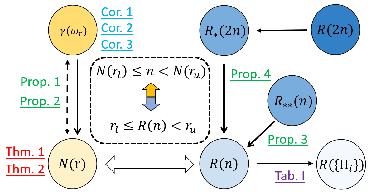
Figure 2: Schematics showing the connections between different quantities in this paper: (a) Left: the relation between simulation cost of Werner states $\gamma(\omega_{r})$ and compatible complexity $N(r)$ for $\mathcal{P}_{r}$; (b) Right: the compatible radius $R(n)$ and its derivatives; (c) The left and right parts are connected by the relation in the middle box; (d) $\rightarrow$(dashed): Upper bound from left to right (in special cases).

As shown in Fig. 2, each input $x$ to the channel corresponds to a local measurement choice for Alice, which we collectively represent by a family of positive operator-measures (POVMs) $\{M_{a|x}\}_{a,x}$. She receives a classical output $a$ while Bob jointly receives the (unnormalized) quantum output

$$\sigma_{a|x}=\textrm{Tr}_{A}[(M_{a|x}\otimes\mathbb{I})\rho_{AB}]$$ (1)

with probability $q(a|x)=\textrm{Tr}[\sigma_{a|x}]$. It is convenient to denote a c-to-cq channel by the set of labeled quantum outputs $\mathcal{A}=\{\sigma_{a|x}\}$, called a state assemblage, and we write $\rho_{AB}\mapsto\mathcal{A}$ when Eq. (1) holds.

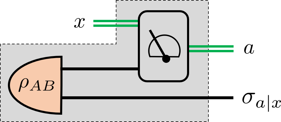
Figure 1: The bipartite state $\rho_{AB}$ is transformed into a c-to-cq channel represented by the assemblage $\mathcal{A}=\{\sigma_{a|x}\}$.

For a given quantum state $\rho_{AB}$, we wish to quantify the amount of classical resources needed to simulate each assemblage $\mathcal{A}$ such that $\rho_{AB}\mapsto\mathcal{A}$. For this simulation task, it is natural to quantify the classical resource in terms of how much shared randomness Alice and Bob need to reproduce $\mathcal{A}$ using a local hidden state (LHS) model. A LHS model for assemblage $\mathcal{A}=\{\sigma_{a|x}\}$, should it exist, is given by a shared random variable $i$ with distribution $p(i)>0$, a family of quantum states $\{\rho_{i}\}$ for Bob, and a classical channel $p(a|x,i)$ for Alice such that

$$\sigma_{a|x}=\sum_{i=1}^{n}p(a|x,i)p(i)\rho_{i}\qquad\forall a,i.$$ (2)

Deploying this model requires Alice and Bob to have shared randomness of size $n\in[1,+\infty]$. For LHS models using a continuous shared variable, the sum in Eq. (2) is replaced with an integral, and an example of this is provided in the Supplemental Material.

If an assemblage $\mathcal{A}$ does not admit a LHS model, then the resource transformation $\rho_{AB}\mapsto\mathcal{A}$ constitutes the celebrated effect of quantum steering [8]. While entanglement is a necessary condition for steering, not all entangled states are steerable. For such states, the next natural question then is to look beyond steering and ask how much shared randomness is needed to simulate all the assemblages that the state can generate. For an unsteerable state $\rho_{AB}$, we define $\gamma(\rho_{AB})\in[1,+\infty]$ as the smallest amount of shared randomness sufficient to simulate any $\mathcal{A}$ such that $\rho_{AB}\mapsto\mathcal{A}$. When Alice holds a qubit, we also define $\gamma^{p}(\rho_{AB})$ as the shared randomness cost for simulating any $\mathcal{A}$ generated by measurements that are confined to the $x-z$ plane.

One important question we consider is whether the simulation cost $\gamma(\rho_{AB})$ satisfies some general dimensionality bound. In fact, we always have $\gamma(\rho_{AB})\leq(\dim(A))^{2}(\dim(B))^{2}$ for every separable state $\rho_{AB}$ due the existence of minimal separable decompositions [11]. However, does this bound also hold for entangled states? This question was first raised and left unanswered by Brunner et al. in a work that explored local models with finite shared randomness [12]. Later, Nguyen et al. proposed a geometric method for characterizing quantum steering that enables a quantification of simulation cost from the other direction, namely by computing states that are unsteerable given a finite amount of shared randomness [13]. These inspirational papers both provide upper bounds on $\gamma(\rho_{AB})$ under projective measurement; however, computable lower bounds have been missing, and thus a resource comparison among separable and entangled-unsteerable states cannot yet be made.

In this work, we resolve the aforementioned question and show that no universal upper bound on simulation costs exists for unsteerable entangled states: i.e., even for two-qubit states $\gamma(\rho_{AB})$ is unbounded. The bulk of our results focus on the two-qubit family of Werner states,

Singlet Weight	SR Cost $\gamma(\omega_{r})$	State Structure
$r=0$	$\gamma=1$	product state
$0<r\leq\frac{1}{3}$	$\gamma=4$	separable
$\frac{1}{3}<r\leq\frac{1}{2}$	$\gamma>4\;$ (Cor. 1);	entangled and
	$\gamma=\Omega\big{(}(\frac{1}{2}-r)^{-\frac{2}{5}}\big{)}\;$ (Prop.1)	unsteerable
$\frac{1}{2}<r<1$	—	steerable

Table 1: Simulation cost of two-qubit Werner-states $\omega_{r}$.

$$\omega_{r}=r|\Psi^{-}\rangle\langle\Psi^{-}|+(1-r)\frac{\mathbb{I}\otimes\mathbb{I}}{4},$$ (3)

where $|\Psi^{-}\rangle=\sqrt{1/2}(|01\rangle-|10\rangle)$ is the singlet state. Our restriction to this simple of family of states may seem like a limitation. However, on the contrary, we show that the many interesting properties simulation cost can already be demonstrated using these states, and they are summarized in Table 1. Furthermore, as we demonstrate in this letter, the lower bounds we prove on $\gamma(\omega_{r})$ translate into lower bounds on $\gamma(\rho_{AB})$ for any unsteerable state $\rho_{AB}$. Finally, the elegant mathematical structure of Werner states allows us to equivalently restate the problem of simulating unsteerable Werner states into the problem of simulating noisy spin measurements; this opens a pathway for using tools in Banach space theory to tackle both problems simultaneously. We proceed now by exploring this equivalence in more detail.

The compatibility of noisy spin measurements – The task of quantum steering is fundamentally related to another quantum phenomenon known as measurement incompatibility [14, 15, 16]. A family of measurements $\{M_{a|x}\}_{a,x}$ is called compatible or jointly measurable if each measurement in the family can be simulated by a single “parent” POVM $\{\Pi_{i}\}_{i=1}^{n}$, in the sense that

$$M_{a|x}=\sum_{i=1}^{n}p(a|x,i)\Pi_{i}\qquad\forall a,i$$ (4)

for some channel $p(a|x,i)$ [17, 18]. In the simple case of quantum observables, compatibility amounts to pairwise commutativity, but the latter is not necessary for general POVMs. For a qubit system, let $\mathcal{P}_{r}$ denote the entire family of “noisy spin measurements.” Each measurement in this family is a two-outcome POVM $\{M_{+|r\hat{n}},M_{-|r\hat{n}}\}$ with $M_{\pm|r\hat{n}}=\tfrac{1}{2}(\mathbb{I}\pm r\hat{n}\cdot\vec{\sigma})$, where $\hat{n}$ is a normalized Bloch vector and $r\in[0,1]$ is the noise parameter which effectively shrinks the Bloch sphere down to radius $r$. We similarly let $\mathcal{P}_{r}^{p}$ denote the subset of all noisy spin measurements with $\hat{n}$ confined to the $x-z$ plane. Note that $\mathcal{P}_{1}$ is the entire family of qubit projective measurements. It has been previously shown that $\mathcal{P}_{r}$ is a compatible family iff $r\in[0,\frac{1}{2}]$ [8, 19], whereas the compatibility range for $\mathcal{P}_{r}^{p}$ is $r\in[0,\frac{2}{\pi}]$ [20].

Skrzypczyk et al. have introduced the notion of compatibility complexity, which for a family of compatible measurements is the smallest number of outcomes $n$ such that Eq. (4) holds [21]. We let $N(r)$ and $N^{p}(r)$ denote the compatibility complexities for measurement families $\mathcal{P}_{r}$ and $\mathcal{P}^{p}_{r}$ in their respective compatibility regions. The connection to the simulation cost of Werner states is given by the following propositions.

Proposition 1.

Suppose that transformation $\omega_{r}\mapsto\mathcal{A}$ is generated by measurement family $\mathcal{P}_{1}$ on Alice side. Then $\mathcal{A}$ can be simulated by shared randomness of size $N(r)$ for $r\in[0,\frac{1}{2}]$. Hence, $\gamma(\omega_{r})\geq N(r)$.

The inequality $\gamma(\omega_{r})\geq N(r)$ follows from the first statement of the proposition since $\gamma(\omega_{r})$ is the simulation cost for arbitrary POVMs on Alice’s side, which includes projective measurements $(\mathcal{P}_{1})$ as a special subfamily. In fact, we show in the Supplemental Material that this inequality is tight for general planar measurements.

Proposition 2.

$\gamma^{p}(\omega_{r})=N^{p}(r)$ for $r\in[0,\frac{2}{\pi}]$.

The compatibility radius – Propositions 1 and 2 directly translate the problem of simulating $\omega_{r}$ into the problem of simulating noisy spin measurements. By definition, $N(r)$ is the smallest integer $n$ such that an $n$-outcome POVM can simulate the measurement family $\mathcal{P}_{r}$ (as in Eq. (4)). But we can turn the quantities around and identify $R(n)$ as the largest $r$ such that an $n$-outcome POVM can simulate $\mathcal{P}_{r}$. We will refer to $R(n)$ as the $n$-outcome compatibility radius. For any $r,r^{\prime}\in[0,\frac{1}{2}]$ and integer $n$, the definitions of $R(n)$ and $N(r)$ imply the relationship

$$r\leq R(n)<r^{\prime}\;\;\Leftrightarrow\;\;N(r)\leq n<N(r^{\prime}).$$ (5)

Similarly, we define $N^{p}(r)$ for the plane-restricted case, and so $r\leq R^{p}(n)<r^{\prime}\;\Leftrightarrow\;N^{p}(r)\leq n<N^{p}(r^{\prime})$. From Propositions 1 and 2, we can thus attain bounds for $\gamma(\omega_{r})$ and $\gamma^{p}(\omega_{r})$ through the study of $R(n)$ and $R^{p}(n)$.

For an arbitrary qubit POVM $\{\Pi_{i}\}_{i}$, let $R(\{\Pi_{i}\})$ denote the largest $r$ such that $\{\Pi_{i}\}$ can simulate $\mathcal{P}_{r}$ (and likewise for $R^{p}(\{\Pi_{i}\})$). This notation is similar to the critical radius defined in [13] for quantum steering. The $n$-outcome compatibility radius $R(n)$ is hence the largest $R(\{\Pi_{i}\})$ among all $n$-outcome POVMs $\{\Pi_{i}\}_{i}$. To compute $R(\{\Pi_{i}\})$, we write each $\Pi_{i}$ as in the Pauli basis as

$$\Pi_{i}=\alpha_{i}(\mathbb{I}+\eta_{i}\hat{n}_{i}\cdot\vec{\sigma}),$$ (6)

with $0\leq\eta_{i},\alpha_{i}\leq 1$, and completion constraints $\sum_{i}\alpha_{i}=1$ and $\sum_{i}\alpha_{i}\eta_{i}\hat{n}_{i}=\vec{0}$. In the Supplemental Material, we argue that it is sufficient to consider $\eta_{i}=1$.

From a geometric perspective, $R(\{\Pi_{i}\})$ is determined by the largest $r$ such that the shrunken Bloch sphere of radius $r$ belongs to the set

$$\mathfrak{m}_{\{\Pi_{i}\}}=\left\{2\textstyle\sum_{i}q_{i}\alpha_{i}\hat{n}_{i}\;\big{|}\;0\leq q_{i}\leq 1,\;\sum_{i}q_{i}\alpha_{i}=\tfrac{1}{2}\right\},$$ (7)

which represents the compatible region consisting of all unbiased measurements that can be simulated by $\{\Pi_{i}\}$. By dropping the constraint $\sum_{i}q_{i}\alpha_{i}=\tfrac{1}{2}$, we have an outer approximation set given by

$$\mathfrak{m}^{*}_{\{\Pi_{i}\}}=\left\{2\textstyle\sum_{i}q_{i}\alpha_{i}\hat{n}_{i}\;\big{|}\;0\leq q_{i}\leq 1\right\},$$ (8)

which can also be interpreted exactly as the compatible region of the $2n$-outcome POVM $\textbf{sym}\{\Pi_{i}\}_{i}$ symmetrized form of $\{\Pi_{i}\}$,

$$\textbf{sym}\{\Pi_{i}\}_{i}:=\{\tfrac{\alpha_{i}}{2}(\mathbb{I}+\hat{n}_{i}\cdot\vec{\sigma}),\tfrac{\alpha_{i}}{2}(\mathbb{I}-\hat{n}_{i}\cdot\vec{\sigma})\}_{i}.$$ (9)

The set $\mathfrak{m}^{*}_{\{\Pi_{i}\}}$ is called a zonotope generated by vectors $\{2\alpha_{i}\hat{n}_{i}\}$ [22, 23]. Letting $B^{3}$ denote the unit ball in $\mathbb{R}^{3}$, we arrive at the geometrical characterization.

$$R(\{\Pi_{i}\})=\text{inr}(\mathfrak{m}_{\{\Pi_{i}\}})\leq\text{inr}(\mathfrak{m}^{*}_{\{\Pi_{i}\}}),$$ (10)

where $\text{inr}(S)=\max\{r\;|\;rB^{3}\subset S\}$ is called the inradius of a general convex set $S\subset\mathbb{R}^{3}$. Since $\text{inr}(\mathfrak{m}^{*}_{\{\Pi_{i}\}})$ is the compatible region of $\textbf{sym}\{\Pi_{i}\}_{i}$, we thus obtain

$$R(n)\leq\max_{\{\Pi_{i}\}_{i=1}^{n}}\text{inr}(\mathfrak{m}^{*}_{\{\Pi_{i}\}})=:R_{*}(n)\leq R(2n),$$ (11)

which can be used to find lower and upper bounds on $R(n)$. Below we state our results, saving proofs for the Supplemental Material.

Lower bounding the simulation cost – From Eq. (5), we obtain lower bounds on $\gamma(\omega_{r})$ through upper bounds on $R(n)$. We first draw attention to the case of $n=3$, for which a tight upper bound can be found by a simple geometrical argument. The well-known circumradius-inradius inequality says that the inradius of an $n$-simplex is at least $n$ times less than its circumradius [24]. To apply this, for any three-outcome POVM $\{\Pi_{i}\}_{i=1}^{3}$ observe that the set $\mathfrak{m}_{\{\Pi_{i}\}}$ is contained in the $2$-simplex $\mathfrak{m}^{**}_{\{\Pi_{i}\}}=\{\sum_{i=1}^{3}p_{i}\hat{n}_{i}\;|\;\sum_{i=1}^{3}p_{i}=1\}$, with a circumradius equaling one since the $\hat{n}_{i}$ are unit vectors. Therefore, the circumradius-inradius inequality implies that

$$R(3)=R^{p}(3)\leq\max_{\{\Pi_{i}\}_{i=1}^{3}}\!\text{inr}(\mathfrak{m}^{**}_{\{\Pi_{i}\}})=:R_{**}(3)\leq\frac{1}{2}.$$

A similar argument for four-outcome POVMs on the full Bloch sphere shows that $R(4)\leq\frac{1}{3}$. Combined with the lower bounds of $R(n)$ in the next section (see Table 2), we have

Proposition 3.

$R^{p}(3)=\tfrac{1}{2}$ and $R(4)=\tfrac{1}{3}$.

Corollary 1.

For any $r>\tfrac{1}{3}$, we have $\gamma(\omega_{r})>4$. The simulation cost of any entangled Werner state is strictly greater than that of a separable Werner state.

Unfortunately, the outer approximation $R_{**}(n)$ is too loose for arbitrary $n$. To handle the case of $n>4$ for planar measurements, we can apply the isoperimetric inequality of polygon to obtain the following.

Proposition 4.

$R^{p}(n)\leq\frac{1}{n}\cot(\frac{\pi}{2n})$.

Corollary 2.

For any $r\in[0,\frac{2}{\pi}]$,

$$\gamma^{p}(\omega_{r})=N^{p}(r)\geq\sqrt{\frac{\pi}{6}}\left(\frac{2}{\pi}-r\right)^{-1/2}.$$ (12)

For measurements on the full Bloch sphere, we rely on more sophisticated isoperimetric inequalities of zonotopes [25, 26]. The culminating result is stated in the following theorem.

Theorem 1.

For any $r\in[0,\frac{1}{2}]$,

$$\gamma(\omega_{r})\geq N(r)>c\left(\frac{1}{2}-r\right)^{-2/5}$$ (13)

for some positive constant $c$.

Both Corollary 2 and Theorem 1 establish our primary claim that the simulation cost of an unsteerable entangled state diverges at $r=\tfrac{1}{2}$ (resp. $\frac{2}{\pi}$) when considering general measurements (resp. planar measurements).

Upper bounding the simulation cost – We now turn to the problem of upper bounding the shared randomness cost of unsteerable $\omega_{r}$. Propositions 1 and 2 can again be used to partially solve this problem. Namely, whenever Alice performs projective measurements or planar POVMs we have that the result assemblage $\mathcal{A}$ can be simulated by shared randomness of size $N(r)$ and $N^{p}(r)$ respectively. What about the most general setting of arbitrary POVMs on Alice’s side? Unfortunately, our developed methods appear insufficient to tackle this case, and we leave the full upper bounding as an open problem. However, we note that even if simulating general POVMs requires shared randomness than simulating just projective measurements, the unsteerability range is the same. That is, as we have shown in a companion paper, $\omega_{r}$ is unsteerable under arbitrary POVMs iff unsteerable under arbitrary projective measurements iff $r\in[0,\frac{1}{2}]$ .

Like before, we use Eq. (5) and turn the problem of upper bounding $N(r)$ into lower bounding $R(n)$. The latter is further lower bounded by $R(\{\Pi_{i}\})$ for any specific parent POVM $\{\Pi_{i}\}$. The same reasoning holds for the planar case, and we first consider the rotationally-symmetric planar POVM: $\{\Pi^{\text{rot}}_{i}=1/n(\mathbb{I}+\hat{n}_{i}\cdot\vec{\sigma})\}_{i=1}^{n}$ with $\hat{n}_{i}=\left(\cos(\frac{2\pi i}{n}),0,\sin(\frac{2\pi i}{n})\right)^{T}$ [27]. In the Supplemental Material, we analytically find the compatibility radius to be

$$R^{p}(\{\Pi^{\text{rot}}_{i}\})=\begin{cases}\frac{1}{n}\cot(\frac{\pi}{2n})\cos(\frac{\pi}{2n})~{}~{}&\text{if $n$ is odd}\\ \frac{2}{n}\cot(\frac{\pi}{n})&\text{if $n$ is even}\end{cases},$$ (14)

and a simulation model is explicitly constructed. Similar to the proof of Corollary 2, a Taylor expansion on $\frac{1}{n}\cot(\frac{\pi}{2n})\cos(\frac{\pi}{2n})$ allows us to lower bound $R^{p}(\{\Pi^{\text{rot}}_{i}\})\leq R^{p}(n)$, from which Eq. (5) can be applied to obtain the following.

Corollary 3.

For any $r\in[0,\frac{2}{\pi}]$,

$$\gamma^{p}(\omega_{r})=N^{p}(r)\leq\sqrt{\frac{5\pi}{12}}\left(\frac{2}{\pi}-r\right)^{-1/2}+1,$$ (15)

where the $+1$ term is needed since $R^{p}(\{\Pi^{\text{rot}}_{i}\})$ does not monotonically increase with $n$. This implies that symmetric POVMs do not always have the largest compatibility radius, which disproves a common suggestion made in the literature [13, 28]. We have further confirmed this numerically by searching over arbitrary parent POVMs. As shown in Table 2, for even $n$ a non-symmetric POVM can outperform the rotationally symmetric one. Nevertheless, a comparison of Corollaries 2 and 15 shows that $\{\Pi^{\text{rot}}_{i}\}_{i=1}^{n}$ is near optimal for simulating noisy spin measurements in the $x-z$ plane.

	Planar $R^{p}(n)$		General $R(n)$
n	Symmetric	Numerics	Thomson	Numerics
3	0.5	0.5	0	0
4	0.5	0.5274	0.3333	0.3333
5	0.5854	0.5854	0.3464	0.3716
6	0.5774	0.5927	0.3333	0.4004
7	0.6102	0.6102	0.2857	0.4060
8	0.6035	0.6111	0.4392
9	0.6206	0.6206	0.4446
10	0.6155	0.6213	0.4376
11	0.6259	0.6259	–
12	0.6220	0.6265	0.4588

Table 2: Lower bounds on the compatible radii $R^{p}(n)$ and $R(n)$. For the planar case, the first column describes the largest radius achievable by symmetric POVMs, as given by Eq. (14). For the general case, the third column provides a lower bound on $R(n)$ using solutions to the Thompson problem, while tighter numerical bounds are obtained by random sampling the parent POVM $\{\Pi_{i}\}$[29].

We next turn to simulate arbitrary spin measurements on the shrunken Bloch sphere. In three dimensions, the rotationally-symmetric planar POVM $\{\Pi^{\text{rot}}_{i}\}$ cannot be directly generalized, and so we consider a few alternate approaches. We first use the equally spaced points found in the Thompson problem [30]. The numerical result for $n\in\{4,\cdots 12\}$ is shown in Table. 2. The second construction builds a parent POVM using the symmetries of Platonic solids, and a detailed analysis of this is carried out in the Supplemental Material. The final and most powerful construction uses results from Refs. [25, 31] on zonotope approximations, and is summarized in the following.

Theorem 2.

For any $r\in[0,\frac{1}{2}]$,

$$N(r) \leq C\left(\frac{1}{2}-r\right)^{-4/5}$$ (16)

for some positive constants $C$. Hence, by Proposition 1, the RHS of Eq. (16) also bounds the shared randomness cost for simulating $\omega_{r}$ by projective measurements on Alice’s side.

Simulating general unsteerable states – We now discuss ways in which our results can be applied to unsteerable states beyond the two-qubit Werner family. Observe that any unsteerable state $\rho_{AB}$ will satisfy $\gamma(\rho)\geq\gamma(\mathcal{L}(\rho))-m$ under any map of the form $\mathcal{L}=\sum_{i=1}^{m}\mathcal{N}_{i}\otimes\mathcal{E}_{i}$, where the $\mathcal{N}_{i}$ are completely positive and trace-preserving (CPTP) map while the $\mathcal{E}_{i}$ are just CP [32]. Hence, we can lower bound the simulation cost of $\rho_{AB}$ by first transforming it to a two-qubit state. Then, it is well-known that every two-qubit state can be converted into Werner form when Alice and Bob simultaneously apply one of twelve random Clifford gates to their system (a so-called “twirling map”) [33]. Moreover, the noise parameter $r$ in the resulting state is given by the singlet fraction, i.e. $\rho\mapsto\rho_{W}(r)$ with $r=\langle\Phi^{-}|\rho|\Phi^{-}\rangle-\frac{1}{4}$. Since the twirling map will increase the shared randomness in a LHS model by a factor of twelve, we conclude that any unsteerable state $\rho_{AB}$ with $\langle\Phi^{-}|\mathcal{L}(\rho)|\Phi^{-}\rangle>\mathcal{R}(n)$ will require a LHS model with at least $\log_{2}n-\log_{2}(12m)$ bits of shared randomness. From Theorem 16, this amount grows unbounded as $\langle\Phi^{-}|\mathcal{L}(\rho)|\Phi^{-}\rangle\to 3/4$.

Corollary 1 shows that the separability threshold for two-qubit Werner states coincides with a jump in shared randomness cost from $2$ to $\log_{2}5$ bits. In fact, this connection between separability and unsteerability holds for all two-qubit states $\rho_{AB}$: $\gamma(\rho_{AB})>4$ iff $\rho_{AB}$ is unsteerable and entangled. As explained in the Supplemental Material, this previously unrecognized result actually follows directly from the “nested tetrahedron” condition by Jevtic, et al. [34], and the “four-packable” condition by Nguyen and Vu [35].

Conclusions – In this work we studied the shared randomness cost $\gamma(\rho_{AB})$ for simulating c-to-cq channels built using $\rho_{AB}$. The mathematical methods we developed to study this problem used the correspondence between steerability and measurement incompatibility and their similar geometric picture. Analogous to any other type of channel simulation cost, the quantity $\gamma(\rho_{AB})$ provides one measure of operational resourcefulness for every unsteerable state $\rho$. Furthermore, understanding the simulation cost for different assemblages can be used for semi-device-independent entanglement verification [9] when Alice and Bob are known to have a limited amount of shared randomness, even in noisy environments where quantum steering is not possible.

The results presented here pertain LHS models. As future work, it would be interesting if similar techniques can be applied to bound the shared randomness needed for local hidden variable (LHV) models. Since LHS models are more demanding than LHV models, the upper bounds presented in this work will still apply.

Finally, we close by conjecturing a more fundamental role for the simulation cost $\gamma(\rho_{AB})$ in the study of nonlocality and entanglement. The notion of steerability provides a clean partitioning in the set of bipartite quantum states between those that are steerable versus those that are not. However, this partition does not coincide with the separation between entangled and separable states [36, 8]. In contrast, we have found here that the for two-qubit states the jump from separable to entangled-unsteerable coincides with a jump in the simulation cost. Hence by moving beyond steering and focusing on simulation cost, we recover the separable/entangled boundary. Perhaps such a relationship holds for higher-dimensional bipartite states as well.

Acknowledgements – This work was supported by NSF Award 1839177. The authors thank Virginia Lorenz and Marius Junge for helpful discussions during the preparation of this manuscript.

I Supplementary material

Contents

1. I Supplementary material
   1. I.1 Geometry of compatible region
   2. I.2 Proof of Proposition 2
   3. I.3 Proof of Proposition 3, Corollary 1 and discussion on general entangled state
   4. I.4 Proof of Proposition 4 and Corollary 2
   5. I.5 Proof of Theorem 1 and Theorem  and connection to Zonotope approximation
   6. I.6 Criteria for compatible radius $R(\{\Pi_{i}\})$
   7. I.7 Example of $R(\{\Pi_{i}\})$ for symmetric POVMs, and compatible models
   8. I.8 Connection to quantum steering

Here we provide some technical detail that complements the main manuscript. In Section I.1 we give a detailed geometrical description of our problem in terms of zonotope. In Section I.2, we prove Proposition 2 of the main text. In Section I.3, we prove Proposition 3 and Corollary 1 of the main text, and a generalization of these results to all two-qubit entangled states is given. In Section I.4, we prove Proposition 3 and Corollary 2 of the main text. In Section I.5, we connect our problem to the study of zonotope approximation and Theorems 1 and 2 are proven. In Section I.6 we provide a detailed construction of the compatible radius for a given $\{\Pi_{i}\}$ as an optimization-based criteria. In Section. I.7, we focus closely on some symmetric POVMs and calculate their compatibility region $\mathfrak{m}_{\{\Pi_{i}\}}$ and compatibility radius $R({\{\Pi_{i}\}})$ explicitly. Constructions of compatible models for specific POVMs are also given. Finally, in Section I.8 we establish a connection between our problem and the shared randomness cost in quantum steering.

symbol	Explanation
POVM	Positive-Operator Valued Measurement
PM	Projective Measurement
$\{\Pi_{i}\}_{i\in\mathcal{I}}$	Parent POVM, $\Pi_{i}$ are its effects
$\text{sym}\{\Pi_{i}\}_{i\in\mathcal{I}}$	Symmetric extended Parent POVM
$\mathcal{I}$	Index set of measurement outcome
$\{M_{a|x}\}_{a,x}$	Set of Children POVMs
$\gamma(\omega_{r})$	Simulation cost of Werner state
$N(r)$	Compatible complexity for all PMs
$\mathfrak{M}_{\{\Pi_{i}\}}$	Compatible region of POVM $\{\Pi_{i}\}$
$\mathfrak{m}_{\{\Pi_{i}\}}$	PM Compatible region of POVM $\{\Pi_{i}\}$
$\mathfrak{m}^{*}_{\{\Pi_{i}\}}$	PM Compatible region of POVM $\text{sym}\{\Pi_{i}\}$
$R(\{\Pi_{i}\})$	Compatible radius of the compatible region
$R(n)$	Largest compatible radius for all $n$-outcome POVM
$R_{*}(n)$	Upper bound of $R(n)$ with symmetric extension
$R_{**}(n)$	Upper bound of $R(n)$ with simplex
$\vec{a}$	3-d vector
$\hat{a}$	Unit 3-d vector
$X^{p}$	Quantity for the planar case

Table 3: Notation used throughout the paper and Supplemental Material

I.1 Geometry of compatible region

Definition 1.

A zonotope is a set of points in $d$-dimensional space constructed from vectors $\{\vec{v}_{i}\}$ by taking the Minkowski sum of line segments:

$$\mathcal{Z}=\left\{\sum_{i}x_{i}\vec{v}_{i}|0\leq x_{i}\leq 1\right\},$$

where the set of vectors $\{\vec{v}_{i}\}$ is defined as the generator of the zonotope.

When parameterizing a quantum measurement $\{\Pi_{i}\}$ in the Pauli basis, each effect $\Pi_{i}=\alpha_{i}(\mathbb{I}+\hat{n}_{i}\cdot\vec{\sigma})$ can be written as a 4-d vector:

$$\vec{\pi}_{i}=(\alpha_{i},\alpha_{i}\hat{n}_{i})^{T}=(\alpha_{i},\alpha_{i}\hat{n}_{i}^{x},\alpha_{i}\hat{n}_{i}^{y},\alpha_{i}\hat{n}_{i}^{z})^{T}.$$ (17)

The normalization and positivity constraints are expressed as$\sum_{i}\vec{\pi}_{i}=(1,0,0,0)$ and $\alpha_{i}\geq 0$.

With the above notation, we introduce the compatible region $\mathcal{M}_{\{\Pi_{i}\}}:=\left\{\sum_{i}p_{i}\Pi_{i}\bigg{|}0\leq p_{i}\leq 1\right\}$, which is the collection of all dichotomic measurements generated by $\{\Pi_{i}\}$. This can be presented as a zonotope in 4-dimensional space [22, 23]:

$$\mathfrak{M}_{\{\Pi_{i}\}}:=\left\{2\sum_{i}p_{i}\vec{\pi}_{i}\bigg{|}0\leq p_{i}\leq 1\right\},$$ (18)

where the factor of 2 is introduced for convenience. The two 3-dimensional compatible regions $\mathfrak{m}_{\{\Pi_{i}\}}$ and $\mathfrak{m}_{\{\Pi_{i}\}}^{*}$ we defined in the main text can both be derived from this 4-dimensional zonotope.

Property 1.

The constrained zonotope $\mathfrak{m}_{\{\Pi_{i}\}}:=\left\{2\sum_{i}p_{i}\hat{n}_{i}\bigg{|}0\leq p_{i}\leq 1,\sum_{i}p_{i}\alpha_{i}=\frac{1}{2}\right\}$ is the three-dimensional cross-section of $\mathfrak{M}_{\{\Pi_{i}\}}$ on the plane $\sum_{i}p_{i}\alpha_{i}=\frac{1}{2}$. This, however, is not a zonotope in general [37]. The set $\mathfrak{m}_{\{\Pi_{i}\}}$ represents all unbiased dichotomic measurements that can be simulated by $\{\Pi_{i}\}$.

Property 2.

The projected zonotope $\mathfrak{m}^{*}_{\{\Pi_{i}\}}:=\left\{2\sum_{i}p_{i}\mathbb{P}\vec{\pi}_{i}\bigg{|}0\leq p_{i}\leq 1\right\}=\left\{2\sum_{i}p_{i}\hat{n}_{i}\bigg{|}0\leq p_{i}\leq 1\right\}$ is a zonotope, where $\mathbb{P}$ projects vector $(x,\vec{y})^{T}\in\mathbb{R}^{4}$ onto $(\vec{y})^{T}\in\mathbb{R}^{3}$. By definition, $\mathfrak{m}_{\{\Pi_{i}\}}\subseteq\mathfrak{m}^{*}_{\{\Pi_{i}\}}$ with equality holding if $\{\mathbb{P}\vec{\pi}_{i}\}=\{(\alpha_{i}\hat{n}_{i})^{T}\}$ is central symmetric. Centrally symmetric measurements are the POVMs $\textbf{sym}\{\Pi_{i}\}$ introduced in the main text.

Remark.

The introduction of a projected zonotope is meaningful both geometrically and analytically.

• Geometrically, giving any arbitrary POVM $\{\Pi_{i}\}$, we can symmetrically extend it to a new POVM $\textbf{sym}\{\Pi_{i}\}=\{\frac{\Pi_{i}}{2},(\textrm{Tr}\Pi_{i})\mathbb{I}-\frac{\Pi_{i}}{2}\}$. The projected zonotope for the original POVM is actually the constrained zonotope of the new symmetric-extended POVM $\textbf{sym}\{\Pi_{i}\}$.

• Analytically, when computing the compatibility radius $R(\{\Pi_{i}\})=\inf_{\begin{subarray}{c}|\vec{c}|=1,-1\leq c_{0}\leq 1\end{subarray}}\sum_{i}|\alpha_{i}(c_{0}+\vec{c}\cdot\hat{n}_{i})|$ for the constrained zonotope (see Section I.6), an upper bound is given by the compatible radius for the projected zonotope: $R(\{\Pi_{i}\})\leq R_{*}(\{\Pi_{i}\}):=\inf_{\begin{subarray}{c}|\vec{c}|=1\end{subarray}}\sum_{i}|\alpha_{i}(\vec{c}\cdot\hat{n}_{i})|$.

I.2 Proof of Proposition 2

Now, we give a proof of Proposition 2 in the main text, which relates the compatible complexity of noisy planar projective measurements (PMs) and positive operator-valued measurements (POVMs). We let $R_{\text{POVM}}(n)$ in this section denote the compatible radius for all $n$-outcome noisy POVMs. The latter refers to POVMs of the form $M_{a}^{r}=rM_{a}+(1-r)\frac{\textrm{Tr}(M_{a})}{2}\mathbb{I}$, where $\{M_{a}\}$ is an initial noiseless POVM.

Lemma 1.

$R^{p}_{\text{POVM}}(3)=R^{p}(3)$ and $\gamma^{p}(\omega_{\frac{1}{2}})=N^{p}(\frac{1}{2})$.

Proof.

$R^{p}_{\text{POVM}}(3)\leq R^{p}(3)$ is obvious since PMs form a subset of POVMs.

To show $R^{p}_{\text{POVM}}(3)\geq R^{p}(3)$, first notice that $R^{p}(3)$ has to be obtained by a three-outcome parent $\{\Pi_{i}\}$ with linear independent effects, since $R^{p}(3)=0$ otherwise. Now consider any planar POVM $\{M^{r}_{a}\}$. It suffices to consider three outcome measurements since they are extreme in the $x-z$ plane. Each of its effects $M_{a}^{r}$ forms a two-outcome POVM $\{M_{a}^{r},\mathbb{I}-M_{a}^{r}\}$ which can be simulated by $\{\Pi_{i}\}$ for all $r\leq R^{p}(3)$ since two-outcome POVMs lie in the convex hull of $\mathcal{P}_{r}$. Therefore there exists $0\leq p(a|i)\leq 1$ such that $M^{r}_{a}=\sum_{i=1}^{3}p(a|i)\Pi_{i}$.

Now considering the two normalization conditions, $\sum_{a=1}^{3}M^{r}_{a}=\sum_{i=1}^{3}\Pi_{i}=\mathbb{I}$, we have

$$\sum_{i=1}^{3}(1-\sum_{a}p(a|i))\Pi_{i}=0.$$ (19)

The linearly independence of the $\Pi_{i}$ implies that $\sum_{a}p(a|i)=1$. Hence, the full POVM $\{M^{r}_{a}\}$ can be simulated by $\{\Pi_{i}\}$, and therefore, $R^{p}_{\text{POVM}}(3)\geq R^{p}(3)$. Combined with Prop. 3 we conclude that $R^{p}_{\text{POVM}}(3)=R^{p}(3)=\frac{1}{2}$. This further implies $\gamma^{p}(\rho_{W}(\frac{1}{2}))=\gamma(\rho_{W}(\frac{1}{2}))=3$. ∎

By a similar argument, one can show that

Corollary 4.

$R_{\text{POVM}}(4)=R(4)$ and $\gamma(\omega_{\frac{1}{3}})=N(\frac{1}{3})$.

We now move onto general $n$ in the planar case.

Proposition 2.

$R_{\text{POVM}}^{p}(n)=R^{p}(n)$ and $\gamma^{p}(\omega_{r})=N(r)$.

Proof.

Assume POVM $\{\Pi_{i}\}$ can simulate 2-outcome measurement $\{M^{r}_{a},\mathbb{I}-M^{r}_{a}\}$ so that $M^{r}_{a}=\sum_{i=1}^{n}p(a|i)\Pi_{i}$. We then have

$$\sum_{i=1}^{n}\Pi_{i}=\sum_{a=1}^{3}M_{a}=\mathbb{I}\Longrightarrow(\sum_{a=1}^{3}p(a|i)-1)\Pi_{i}=0.$$ (20)

Thus, it is sufficient to show that there exists a set of coefficient $p(a|i)$ such that $\sum_{a=1}^{3}p(a|i)=1$ for all $i$
For $n=3$: As given in lem. 1, for linear independent $\{\Pi_{i}\}_{i=1}^{3}$ we have $\sum_{a}p(a|i)=1$
For $n=4$: Since $\sum_{a=1}^{3}p(a|i)=1$ does not hold in general, we want to smooth $p(a|i)$ such that $\sum_{a=1}^{3}p(a|i)=1$
Case 1: If any of the $\Pi_{i}$ satisfy $\sum_{a}p(a|i)=1$, then the problem reduces to the case of $n=3$. Thus $\sum_{a=1}^{3}p(a|i)=1$ for all $i$.
Case 2: If none of the $\Pi_{i}$ satisfy $\sum_{a}p(a|i)=1$, up to some index relabeling, their linear dependence is given as:

$$\sum_{i}q_{i}\Pi_{i}=0~{}~{}\text{with}~{}~{} q_{i}:=\sum_{a}p(a|i)-1>0,~{}~{}i=1,2$$

$$q_{i}:=\sum_{a}p(a|i)-1<0,~{}~{}i=3,4$$ (21)

Since $\sum_{a}p(a|i)>1$ for $i=1,2$ , there must exist at least one $a\in\{1,2,3\}$, such that both elements $p(a|1)>0$ and $p(a|2)>0$. We can now construct $M_{a}^{r}$ as

$$M_{a}^{r}=\sum_{i}p(a|i)\Pi_{i}-\beta\sum_{i}q_{i}\Pi_{i}\Longrightarrow\sum_{i}p(a|i)\Pi_{i}$$ (22)

where $\beta>0$ is arbitrary. However, we need to choose $\beta$ such that the new $p(a|i):=p(a|i)-\beta q_{i}$ are valid response functions. When increasing $\beta$ from 0, we encounter two different sub-cases depending on which case happens first:
Case 2a: $\sum_{a}p(a|i)=1$ for some $i$. Then move to Case 1.
Case 2b: $p(a|i)=0$ at first for $i=1,2$. This is possible since $p(a|i)$ is decreasing for $i=1,2$. Without loss of generality, let’s assume $p(a|1)=0$. Since $\sum_{a}p(a|1)>1$, for all $a^{\prime}\neq a$ we still must have $p(a^{\prime}|1)>0$ (there are non-zero elements to ensure the sum is greater than 1). Therefore, one can find an $a^{\prime}$ such that $p({a^{\prime}|1})>0$ and $p({a^{\prime}|2})>0$. We then repeat Case 2, either arriving at Case 2a or Case 2b. Since $a\in\{1,2,3\}$ and each instance of Case 2b sets a new value $p(a|i)=0$ for $i=1,2$, we can only apply Case 2b at most twice before arriving to Case 2a. Hence, in the end, we will always be able to construct a suitable $p(a|i)$ such that $0\leq p(a|i)\leq 1$ and $\sum_{a}p(a|i)=1$
For $n\geq 5$: Assuming $\sum_{a}p(a|i)\neq 1$ for all $i$. We can divide these effects in two indexed sets $\mathcal{J}$ and $\mathcal{K}$ based on the sign of $q_{i}$. Since we’re in the plane, there must exist two pair of $\Pi_{i}$ taken from $\mathcal{J}$ and $\mathcal{K}$, respectively, such that

$$\sum_{i}q_{i}\Pi_{i}:=t_{j_{1}}\Pi_{j_{1}}+t_{j_{2}}\Pi_{j_{2}}-t_{k_{1}}\Pi_{k_{1}}-t_{k_{2}}\Pi_{k_{2}}=0$$

With this linear dependent relation, we can follow the same procedure as in $n=4$ iteratively and smooth $\sum_{a}p(a|i)=1$ one by one until we get $n=3$. ∎

I.3 Proof of Proposition 3, Corollary 1 and discussion on general entangled state

Lemma 2 (The circumradius-Inradius inequality).

The inradius $r$ of an arbitary $n$-simplex is at least $n$ times less than it circumradius $R$. The inequality saturates when the $n$-simplex is regular.

Proof.

Let $A_{i}$ and $F_{i}$ (for $i=1,2,...,n+1$) denote, respectively, the vertices and its opposite $(n-1)$-dimensional faces of an $n$-dimensional simplex of volume $V$. Also, let $h_{i}$ and $\eta_{i}$ denote the distances from $A_{i}$ and circumcenter $O$ to the $F_{i}$, respectively.

Then $R+\eta_{i}\geq h_{i}$. Moreover, the volume of the $n$-dimensional simplex is given by $h_{i}F_{i}/n$, and so by evaluating the volume of the simplex in three different ways, we get:

$$nV=h_{i}F_{i}=\sum\eta_{i}F_{i}=r\sum F_{i}.$$

Therefore,

$$\sum(R+\eta_{i})F_{i}=(R+r)\sum F_{i}\geq\sum h_{i}F_{i}=(n+1)r\sum F_{i}\rightarrow R\geq nr$$

∎

Proposition 3.

$\mathcal{R}^{p}(3)=\tfrac{1}{2}$ and $\mathcal{R}(4)=\tfrac{1}{3}$.

Proof.

To apply Lemma 2, first consider the planar case. Given any three-outcome POVM $\{\Pi_{i}\}_{i=1}^{3}$, observe that the set $\mathfrak{m}_{\{\Pi_{i}\}}$ is contained in the $2$-simplex $\mathfrak{m}^{**}_{\{\Pi_{i}\}}=\{\sum_{i=1}^{3}p_{i}\hat{n}_{i}\;|\;\sum_{i=1}^{3}p_{i}=1\}$ in two dimensions, with a circumradius equaling one since the $\hat{n}_{i}$ are unit vectors. Therefore, the circumradius-inradius inequality implies that

$$\mathcal{R}^{p}(3)\leq\max_{\{\Pi_{i}\}_{i=1}^{3}}\!\text{inr}(\mathfrak{m}^{**}_{\{\Pi_{i}\}})=:\mathcal{R}_{**}^{p}(3)\leq\frac{1}{2}.$$

A similar argument for four-outcome POVMs on the full Bloch sphere shows that $\mathcal{R}(4)\leq\frac{1}{3}$, where now the compatible region $\mathfrak{m}_{\{\Pi_{i}\}}$ and three-simplex $\mathfrak{m}^{**}_{\{\Pi_{i}\}}$ are in $\mathbb{R}^{3}$. Combined with the lower bounds from Table I in the main text, we have the stated equalities. ∎

Corollary 1.

For any $r>\tfrac{1}{3}$, we have $\gamma(\rho_{W}(r))>4$. The simulation cost of any entangled Werner state is strictly greater than that of a separable Werner state.

Corollary 1 shows that any entangled Werner state requires a strictly higher simulation cost than all separable states. Now we will generalize this result to an arbitrary entangled state by restating the “nested tetrahedron” condition proposed in [34].

Lemma 3 ([34]).

A two-qubit state $\rho_{AB}$ is separable if and only if its steering ellipsoid $\mathcal{E}_{A}$ fits inside a tetrahedron that fits inside the Bloch sphere, where the steering ellipsoid $\mathcal{E}_{A}$ for bipartite state $\rho_{AB}$ is defined as follows:

$$\rho_{AB}=\begin{pmatrix}1&\bm{b}^{T}\\ \bm{a}&T\end{pmatrix}\xRightarrow{\text{SLOCC}:~{}~{}\mathbb{I}\otimes(2\rho_{B})^{-1/2}}\tilde{\rho}_{AB}=\begin{pmatrix}1&\bm{0}\\ \bm{\tilde{a}}&\tilde{T}\end{pmatrix}\xRightarrow{M_{\pm|\bm{n}}}\sigma_{\pm|\bm{n}x}=\frac{1}{2}\begin{pmatrix}1\\ \tilde{\bm{a}}\pm\tilde{T}\bm{n}\end{pmatrix}\Rightarrow\mathcal{E}_{A}=\{\tilde{\bm{a}}+\tilde{T}\bm{n}\}_{\bm{n}}$$ (23)

Proposition 5.

$\rho_{AB}$ is entangled if and only if $\gamma(\rho_{AB})>4$.

Proof.

We prove this by contradiction. Since $\rho_{AB}$ is entangled if and only if $\tilde{\rho}_{AB}$ is entangled, assume $\gamma(\tilde{\rho}_{AB})\leq 4$ for entangled state $\tilde{\rho}_{AB}$. Then there exists a set of local hidden states $\{\rho_{i}=\frac{1}{2}(\mathbb{I}+\bm{n}_{i}\cdot\bm{\sigma})\}_{i=1}^{4}$ such that:

$$\sigma_{\pm|\bm{n}}=\sum_{i=1}^{4}p(\pm|\bm{n},i)p(i)\rho_{i}\Rightarrow\mathcal{E}_{A}=\{\tilde{\bm{a}}+\tilde{T}\bm{n}\}_{\bm{n}}\subseteq\text{Conv}[\bm{n}_{i}]_{i=1}^{4}.$$ (24)

This essentially shows that there exists a tetrahedron defined by the Bloch vectors $\{\bm{n}_{i}\}_{i=1}^{4}$ of $\{\rho_{i}\}_{i=1}^{4}$ that contain the ellipsoid $\mathcal{E}_{A}$. Thus $\tilde{\rho}_{AB}$ is entangled from Lem. 23, and there is a contradiction. With this we conclude that $\rho_{AB}$ is entangled if and only if $\gamma(\rho_{AB})>4$. ∎

I.4 Proof of Proposition 4 and Corollary 2

Proposition 4.

For $n$-outcome planar measurement, $\mathcal{R}^{p}(n)\leq\frac{1}{n}\cot(\frac{\pi}{2n})$

Let $\{\Pi_{i}\}_{i=1}^{n}$ be an arbitrary $n$-outcome planar POVM. According to Eq. (11), its compatible radius will be upper bounded by the inscribed radius $\mathsf{m}^{*}_{\{\Pi_{i}\}}$, i.e.,

$$R^{p}(n)\leq R_{*}^{p}(n)=\sup_{\{\Pi_{i}\}}\textbf{inr}({\mathsf{m}^{*}_{\{\Pi_{i}\}}})\leq\max_{\{\alpha_{i}\hat{n}_{i}\}}\frac{2A}{L},$$ (25)

where $A$ is the area of a $2n$-sided zonogon with generators $\{2\alpha_{i}\hat{n}_{i}\}$ and perimeter $L=4\sum_{i}\alpha_{i}=4$ (This perimeter always holds, since the polygon consists of $n$ pairs of sides parallel to its generators). The isoperimetric inequality of a such a $2n$-sided polygon [38] stipulates that

$$A\leq\frac{L^{2}}{8n\tan(\frac{\pi}{2n})}.$$ (26)

Therefore, we have the upper bound

$$R^{p}(n)\leq\frac{1}{n}\cot(\frac{\pi}{2n})<\frac{2}{\pi}$$ (27)

By considering a Taylor expansion of $x\cot x$ about $x=0$, we observe the inequality $\frac{1}{n}\cot(\frac{\pi}{2n})\leq\frac{2}{\pi}\left(1-\frac{1}{3}(\frac{\pi}{2n})^{2}\right)$. Setting $r^{\prime}=\frac{2}{\pi}\left(1-\frac{1}{3}(\frac{\pi}{2n})^{2}\right)$, we apply Eq. (5) and Proposition 2 to reach Corollary 2.

Corollary 2.

For any $r\in[0,\frac{2}{\pi}]$,

$$\gamma^{p}(\omega_{r})=N^{p}(r)\geq\sqrt{\frac{\pi}{6}}\left(\frac{2}{\pi}-r\right)^{-1/2}.$$ (28)

I.5 Proof of Theorem 1 and Theorem 2 and connection to Zonotope approximation

In this section, we will discuss the technical details of applying the well-studied results in approximating Euclidean Balls with Zonotopes to our specific problem.

Proposition 5.

[39] For any zonotope generated by $2n$ line segments $\{\pm\alpha_{i}\hat{n}_{i}\}$ with $\sum_{i}\alpha_{i}=1$, There exist a positive constant $c_{d}$ depending on dimension $d$ only such that:

$$\left\lVert\sum_{i}\alpha_{i}|\langle\hat{n}_{i},\hat{x}\rangle|-\beta_{d}\right\rVert_{L^{2}(S_{d-1})}\geq c_{d}n^{-\frac{d+2}{2(d-1)}},$$ (29)

where $\left\lVert X\right\rVert_{L^{2}(S_{d-1})}=\sqrt{\int|x|^{2}dS_{d-1}}$ is the $L^{2}$ norm on the integral of function $x$ and $\beta_{3}=\frac{1}{2}$, $\beta_{2}=\frac{2}{\pi}$.

The proof is given in detail in [39] based on the spherical harmonic expansion of these quantities.

Theorem 1.

For any $n$-outcome POVM $\{\Pi_{i}\}$, the compatible radius is upper bounded by

$$R(n)\leq\frac{1}{2}-c_{3}n^{-\frac{5}{2}} \Longleftrightarrow\gamma(\omega_{r})\geq c^{\prime}_{3}|\frac{1}{2}-r|^{-\frac{2}{5}}$$

$$R^{p}(n)\leq\frac{2}{\pi}-c_{2}n^{-4} \Longleftrightarrow\gamma^{p}(\omega_{r})\geq c^{\prime}_{2}|\frac{2}{\pi}-r|^{-\frac{1}{4}}$$ (30)

for some positive constant $c_{d}$.

Proof.

For any $n$-outcome POVM $\{\Pi_{i}\}$, we have a chain of inequality given as:

$$R(n)=\max_{\{\Pi_{i}\}}R({\{\Pi_{i}\}})\leq\max_{\{\Pi_{i}\}}R({\text{{sym}}\{\Pi_{i}\}})=2\max_{\{\alpha_{i}\hat{n}_{i}\}}\text{inr}(\mathfrak{m}^{*}_{\{\Pi_{i}\}})=\max_{\{\alpha_{i}\hat{n}_{i}\}}\min_{\hat{x}}\sum_{i}\alpha_{i}|\langle\hat{n}_{i},\hat{x}\rangle|$$ (31)

(see Eq. (48) for the last equality). From Proposition 5, we have a lower bound on $\left\lVert\sum_{i}\alpha_{i}|\langle\hat{n}_{i},\hat{x}\rangle|-\beta_{d}\right\rVert_{L^{2}(S_{d-1})}$. Using Holder’s inequality,

$$\left\lVert\sum_{i}\alpha_{i}|\langle\hat{n}_{i},\hat{x}\rangle|-\beta_{d}\right\rVert_{L^{2}(S_{d-1})}^{2} \leq\left\lVert\sum_{i}\alpha_{i}|\langle\hat{n}_{i},\hat{x}\rangle|-\beta_{d}\right\rVert_{L^{1}(S_{d-1})}\left\lVert\sum_{i}\alpha_{i}|\langle\hat{n}_{i},\hat{x}\rangle|-\beta_{d}\right\rVert_{L^{\infty}(S_{d-1})}$$

$$\leq\left\lVert\sum_{i}\alpha_{i}|\langle\hat{n}_{i},\hat{x}\rangle|-\beta_{d}\right\rVert_{L^{1}(S_{d-1})}$$ (32)

Where $L^{1}$, and $L^{\infty}$ stand for the $L^{1}$ and $L^{\infty}$ norm of the integral of measurable function. Additionally, since $\int(\sum_{i}\alpha_{i}|\langle\hat{n}_{i},\hat{x}\rangle|-\beta_{d})dS_{d-1}=0$ implies that

$$\int_{\sum_{i}\alpha_{i}|\langle\hat{n}_{i},\hat{x}\rangle|<\beta_{d}}\left|\sum_{i}\alpha_{i}|\langle\hat{n}_{i},\hat{x}\rangle|-\beta_{d}\right|dS_{2}=\frac{1}{2}\left\lVert\sum_{i}\alpha_{i}|\langle\hat{n}_{i},\hat{x}\rangle|-\beta_{d}\right\rVert_{L^{1}},$$ (33)

we therefore have

$$\max_{\hat{x}}\left(\beta_{d}-\sum_{i}\alpha_{i}|\langle\hat{n}_{i},\hat{x}\rangle|\right)\geq\frac{1}{2}\left\lVert\sum_{i}\alpha_{i}|\langle\hat{n}_{i},\hat{x}\rangle|-\beta_{d}\right\rVert_{L^{1}}\geq\frac{1}{2}\left\lVert\sum_{i}\alpha_{i}|\langle\hat{n}_{i},\hat{x}\rangle|-\beta_{d}\right\rVert_{L^{2}}^{2}\geq\frac{1}{2}c_{d}^{2}n^{-\frac{d+2}{d-1}}.$$ (34)

In the end we have

$$\max_{\{\alpha_{i}\hat{n}_{i}\}}\min_{\hat{x}}\sum_{i}\alpha_{i}|\langle\hat{n}_{i},\hat{x}\rangle|\leq\beta_{d}-\frac{1}{2}c_{d}^{2}n^{-\frac{d+2}{d-1}},$$ (35)

from which we conclude:

$$R(n)\leq R_{*}(2n)\leq\frac{1}{2}-c_{3}^{\prime}n^{-\frac{5}{2}} \Longleftrightarrow\gamma(\omega_{r})\geq c^{\prime}_{3}|\frac{1}{2}-r|^{-\frac{2}{5}}$$

$$R^{p}(n)\leq R^{p}_{*}(2n)\leq\frac{2}{\pi}-c_{2}^{\prime}n^{-4} \Longleftrightarrow\gamma^{p}(\omega_{r})\geq c^{\prime}_{2}|\frac{2}{\pi}-r|^{-\frac{1}{4}}$$

for some positive constant $c_{d}^{\prime}$ ∎

Remark.

The bound here for planar measurements is less tight than the upper bound we obtained in Proposition 4.

Proposition 6 ([31]).

There exists a positive constant $C_{d}$ and zonotope in $\mathbb{R}^{d}$ with $2n$ generators $\{\pm\alpha_{i}\hat{n}_{i}\}_{i=1}^{n}$ such that

$$\left|\sum_{i=1}^{n}\alpha_{i}|\hat{n}_{i}\cdot\hat{c}|-\beta_{d}\right|<C_{d}n^{-\frac{1}{2}-\frac{3}{2(d-1)}}\qquad\forall\hat{c},$$ (37)

where $\beta_{d}=\int_{S_{d-1}}\sum_{i=1}^{n}\alpha_{i}|\hat{n}_{i}\cdot\hat{c}|d\hat{c}/\int_{S_{d-1}}d\hat{c}$, with $\beta_{2}=\tfrac{2}{\pi}$ and $\beta_{3}=\tfrac{1}{2}$.

From Proposition 6, since $\min_{\hat{c}}\sum_{i=1}^{n}\alpha_{i}|(\hat{c}\cdot\hat{n}_{i})|\leq\beta_{d}$ by definition, using Eq. 48 we have

$$\begin{split}R(2n)&\geq R(\text{sym}\{\Pi_{i}\})\\ &=\min_{\hat{c}}\sum_{i=1}^{n}\alpha_{i}|(\hat{c}\cdot\hat{n}_{i})|>\beta_{d}-C_{d}n^{-\frac{1}{2}-\frac{3}{2(d-1)}}.\end{split}$$ (38)

We thus immediately obtain an upper bound on the simulation cost:

Theorem 2.

For $r<\frac{1}{2}$ (resp. $r<\frac{2}{\pi}$), the simulation cost is upper bounded by:

$$\gamma^{p}(\omega_{r}) \leq C^{\prime}_{2}|\frac{1}{2}-r|^{-4/5}$$ (39)

$$\gamma(\omega_{r}) \leq C^{\prime}_{3}|\frac{2}{\pi}-r|^{-1/2}$$ (40)

for some positive constants $C^{\prime}_{d}$.

We note that, for planar measurements, the asymptotic limit can also be obtained by taking $n\rightarrow\infty$ in Eq. 14, which yields: $R(n)\geq R^{p}(\{\Pi_{i}^{\text{rot}}\})\approx\frac{2}{\pi}-\frac{\pi}{6n^{2}}$. Therefore, $\gamma^{p}(\omega_{r})=N^{p}(r)\leq\sqrt{\tfrac{\pi}{6}}|\tfrac{2}{\pi}-r|^{-1/2}$

I.6 Criteria for compatible radius $R(\{\Pi_{i}\})$

Theorem 3.

For a given POVM $\{\Pi_{i}\}$, the compatible radius $R(\{\Pi_{i}\})$ is given by:

$$R(\{\Pi_{i}\})=\inf_{\begin{subarray}{c}|\vec{c}|=1\\ -1\leq c_{0}\leq 1\end{subarray}}\sum_{i}|\alpha_{i}(c_{0}+\eta_{i}\vec{c}\cdot\hat{n}_{i})|.$$ (41)

Proof.

We start by noticing that the set $\mathcal{M}_{\{\Pi_{i}\}}$ is convex for any given $\{\Pi_{i}\}$. Therefore, we can always find a set of tight inequalities that bound $\mathcal{M}_{\{\Pi_{i}\}}$. Such an inequality can be represented using an operator $C=c_{0}\mathbb{I}+\vec{c}\cdot\vec{\sigma}$. Let $N\in\mathcal{M}_{\{\Pi_{i}\}}$, then for any $C$ we can write the inequality as

$$\langle C,N\rangle\leq\max_{{M}\in\mathcal{M}_{\{\Pi_{i}\}}}\langle C,M\rangle$$ (42)

where $\langle X,Y\rangle=\textrm{Tr}[XY]$.

Given a child POVM $N=n_{0}(\mathbb{I}+\vec{n}\cdot\vec{\sigma})$, we can proceed to simplify the above inequality:

$$\begin{split}n_{0}(c_{o}+\vec{c}\cdot\vec{n})&\leq\sum_{i}\max_{0\leq x_{i}\leq 1}\alpha_{i}x_{i}(c_{0}+\eta_{i}\vec{c}\cdot\hat{n}_{i})\\ &=\sum_{i}\max[\alpha_{i}(c_{0}+\eta_{i}\vec{c}\cdot\hat{n}_{i}),0],\end{split}$$ (43)

where the equality is always attainable by setting $x_{i}=0$ whenever $c_{0}+\eta_{i}\vec{c}\cdot\hat{n}_{i}\leq 0$ and $x_{i}=1$ otherwise. Moreover for any $N\in\mathcal{M}_{\{\Pi_{i}\}}$, we have $n_{0}=\frac{1}{2}$. Therefore, we can simplify the above inequality as:

$$\begin{split}\vec{c}\cdot\vec{n}\leq 2\sum_{i}\max[\alpha_{i}(c_{0}+\eta_{i}\vec{c}\cdot\hat{n}_{i}),0]-c_{0}&=2\sum_{i}\max[\alpha_{i}(c_{0}+\eta_{i}\vec{c}\cdot\hat{n}_{i}),0]-\sum_{i}\alpha_{i}c_{0}-\sum_{i}\alpha_{i}\eta_{i}\vec{c}\cdot\hat{n}_{i}\\ &=\sum_{i}|\alpha_{i}(c_{0}+\eta_{i}\vec{c}\cdot\hat{n}_{i})|,\end{split}$$ (44)

where we use $\sum_{i}\alpha_{i}=1~{}\text{and}~{}\sum_{i}\alpha_{i}\eta_{i}\hat{n}_{i}=\vec{0}$ in the first equality.

When varying over all choice of operator $C$ (thus, all inequalities that bound the convex set $\mathcal{M}_{\{\Pi_{i}\}}$), we finally arrive at the criteria:

$$|\vec{n}|\leq\frac{\inf_{c_{0},\vec{c}}\sum_{i}|\alpha_{i}(c_{0}+\eta_{i}\vec{c}\cdot\hat{n}_{i})|}{|\vec{c}|}.$$ (45)

Since we are always allowed to scale $c_{0}$ and $|\vec{c}|$, the above infimum can be further simplified with constraint $|\vec{c}|=1$ and $-1\leq c_{0}\leq 1$:

$$R(\{\Pi_{i}\})=\inf_{\begin{subarray}{c}|\vec{c}|=1\\ -1\leq c_{0}\leq 1\end{subarray}}\sum_{i}|\alpha_{i}(c_{0}+\eta_{i}\vec{c}\cdot\hat{n}_{i})|$$ (46)

The compatibility radius $R(n)$ can then be expressed as

$$R(n)=\sup_{\begin{subarray}{c}\{\Pi_{i}\}\end{subarray}}\inf_{\begin{subarray}{c}|\vec{c}|=1\\ -1\leq c_{0}\leq 1\end{subarray}}\sum_{i}|\alpha_{i}(c_{0}+\eta_{i}\vec{c}\cdot\hat{n}_{i})|,$$ (47)

where the superior is taken over all $n$-element POVMs. ∎

Proposition 6.

$R(n)$ is maximized by rank-1 POVM $\{\Pi_{n}\}$, i.e., $\eta_{i}=1$ for $i\in[n]$.

Proof.

Given any POVM $\{\Pi_{n}\}$ with $\Pi_{i}=\alpha_{i}(\mathbb{I}+\eta_{i}\hat{n}_{i}\cdot\vec{\sigma})$, we can define POVM $\{\Pi^{\prime}_{i}\}$ with:

$$\Pi^{\prime}_{i}=\beta_{i}(\mathbb{I}+\hat{n}_{i}\cdot\vec{\sigma})$$

where $\beta_{i}=\frac{\alpha_{i}\eta_{i}}{\sum_{j}\alpha_{j}\eta_{j}}$. Let $c^{*}_{0}$ and $\vec{c^{*}}$ be such that

$$R(\{\Pi_{i}^{\prime}\})=\inf_{\begin{subarray}{c}|\vec{c}|=1\\ -1\leq c_{0}\leq 1\end{subarray}}\sum_{i}|\beta_{i}(c_{0}+\vec{c}\cdot\hat{n}_{i})|=\sum_{i}|\beta_{i}(c^{*}_{0}+\vec{c^{*}}\cdot\hat{n}_{i})|=\frac{1}{\sum_{j}\alpha_{j}\eta_{j}}\sum_{i}|\alpha_{i}\eta_{i}(c^{*}_{0}+\vec{c^{*}}\cdot\hat{n}_{i})|$$

For each individual term above,

$$|\alpha_{i}\eta_{i}(c^{*}_{0}+\vec{c^{*}}\cdot\hat{n}_{i})|+|(1-\eta_{i})\alpha_{i}c_{0}^{*}|\geq|\alpha_{i}(c^{*}_{0}+\eta_{i}\vec{c^{*}}\cdot\hat{n}_{i})|.$$

Summing over $i$, we have

$$\sum_{i}|\alpha_{i}\eta_{i}(c^{*}_{0}+\vec{c^{*}}\cdot\hat{n}_{i})|+\sum_{i}|(1-\eta_{i})\alpha_{i}c_{0}^{*}|\geq\sum_{i}|\alpha_{i}(c^{*}_{0}+\eta_{i}\vec{c^{*}}\cdot\hat{n}_{i})|,$$

which is equivalent to

$$\sum_{j}\alpha_{j}\eta_{j}R(\{\Pi_{i}^{\prime}\})+(1-\sum_{j}\alpha_{j}\eta_{j})|c_{0}^{*}|\geq\sum_{i}|\alpha_{i}(c^{*}_{0}+\eta_{i}\vec{c^{*}}\cdot\hat{n}_{i})|\geq R(\{\Pi_{i}\}).$$

The last inequality holds because $(c^{*}_{0},\vec{c^{*}})$ might not be the optimal choice for $\{\Pi_{i}\}$.

The last piece of the proof relies on showing $R(\{\Pi_{i}^{\prime}\})\geq|c_{0}^{*}|$. This holds beacuase:

$$R(\{\Pi_{i}^{\prime}\})=\sum_{i}|\beta_{i}(c^{*}_{0}+\vec{c^{*}}\cdot\hat{n}_{i})|\geq|\sum_{i}\beta_{i}(c^{*}_{0}+\vec{c^{*}}\cdot\hat{n}_{i})|=|c^{*}_{0}|$$

Therefore, we finally have:

$$R(\{\Pi_{i}^{\prime}\})\geq R(\{\Pi_{i}\}).$$

∎

Remark.

For symmetric POVM $\text{sym}\{\Pi_{i}\}$, the compatible radius can be computed as

$$R(\text{sym}\{\Pi_{i}\})=\min_{\hat{c}}\sum_{i=1}^{n}\alpha_{i}|(\hat{c}\cdot\hat{n}_{i})|$$ (48)

To show this is true for all symmetrically symmetric POVM, notice that optimization $\inf_{x}(|x+y|+|x-y|)$ is always obtained with $x=0$, thus

$$R(\text{sym}\{\Pi_{i}\})=\inf_{\begin{subarray}{c}|\vec{c}|=1\\ -1\leq c_{0}\leq 1\end{subarray}}\frac{1}{2}[\sum_{i}|\alpha_{i}(c_{0}+\eta_{i}\vec{c}\cdot\hat{n}_{i})|+\sum_{i}|\alpha_{i}(c_{0}-\eta_{i}\vec{c}\cdot\hat{n}_{i})|]=\min_{\hat{c}}\sum_{i=1}^{n}\alpha_{i}|(\hat{c}\cdot\hat{n}_{i})|$$ (49)

Proposition 7.

The Compatible radius $R(\{\Pi_{i}\})$ can be computed by considering a finite set of operators $C=c_{0}\mathbb{I}+\vec{c}\cdot\vec{\sigma}$, where $(c_{0},\vec{c})^{T}$ is defined by the norm vector of facets of $\mathfrak{M}_{\{\Pi_{i}\}}$.

Proof.

As discussed in Section I.1, the compatible region is a convex zonotope. Instead of running over all hyperplane boundaries given by operator $C=c_{0}\mathbb{I}+\vec{c}\cdot\vec{\sigma}$, it suffices to consider a finite set of the operator $C$ that define the normal vectors of those facets. A similar idea has been brought up in [13].

From the property of a zonotope, every edge of the compatible region $\mathfrak{M}_{\{\Pi_{i}\}}$ is always parallel to one of its generator vectors $(1,\hat{n}_{i})$, while each facet is defined by $d-1=3$ edges of the set. Therefore, we just have to consider at most $\binom{n}{3}$ different choices of normal vectors. To be more specific, the vector $(c_{0},\vec{c})$ should be perpendicular to three different vectors $(1,\hat{n}_{i})$. Hence, we can write

$$\vec{c}=\frac{(\hat{n}_{x}-\hat{n}_{y})\times(\hat{n}_{x}-\hat{n}_{z})}{|(\hat{n}_{x}-\hat{n}_{y})\times(\hat{n}_{x}-\hat{n}_{z})|},~{}~{}~{}~{}c_{0}=-\vec{c}\cdot\hat{n}_{x}$$ (50)

where $\hat{n}_{x},\hat{n}_{y}$ and $\hat{n}_{z}$ are any choices of distinct vectors associated to POVM $\{\pi_{i}\}$. Therefore, we can now simplify the criteria above by calculating the minimum value over a finite set of size $\binom{n}{3}$.

Similarly, for the case with planar measurement, the vector $(c_{0},\vec{c})$ should be perpendicular to two different vectors $(1,\hat{n}_{i})^{T}$. Hence we can write:

$$(c_{0},\vec{c})^{T}={(1,\hat{n}_{x})^{T}\times(1,\hat{n}_{y})^{T}}$$ (51)

where $\vec{c},\hat{n}_{i}$ are written as vectors in $\mathbb{R}^{2}$. ∎

I.7 Example of $R(\{\Pi_{i}\})$ for symmetric POVMs, and compatible models

In this section, we compute the compatible radius $R(\{\Pi_{i}\})$ for different classes of symmetric POVMs, including: Result 1: the compatible radius for rotationally symmetric planar measurements; Result 2: a compatible model for rotationally symmetric planar measurements; Result 3: the compatible radius for POVMs with regular polyhedron configuration.

Result 1.

For equally spaced planar measurement ${\Pi^{\text{rot}}_{i}=\frac{1}{n}(\mathbb{I}+\hat{n}_{i}\cdot\sigma)}$ with $\hat{n}_{i}=[\cos(\frac{2\pi i}{n}),0,\sin(\frac{2\pi i}{n})]^{T}$, we have:

$$R^{p}(\{\Pi^{\text{rot}}_{i}\})=\begin{cases}\frac{1}{n}\cot(\frac{\pi}{2n})\cos(\frac{\pi}{2n})~{}~{}~{}~{}&\text{if $n$ is odd}\\ \frac{2}{n}\cot(\frac{\pi}{n})&\text{if $n$ is even}.\end{cases}$$ (52)

Proof.

If $n$ is even, the original vectors $\hat{n}_{i}$ form a regular polygon with $n$ sides. To get the extreme point $M^{n}_{i}\in\mathcal{M}_{\{\Pi_{i}\}}$, we can simply add up half of $\{\Pi^{\text{rot}}_{i}\}$ and obtain:

$$M^{n}_{i}=\sum_{j=i}^{j=n/2+i-1}\Pi^{\text{rot}}_{j}=\frac{1}{2}(\mathbb{I}+\vec{m}_{i}\cdot\sigma)$$ (53)

where $\{\vec{m}_{i}\}$ form exactly the same regular polygon with $|\vec{m}_{i}|=\frac{2}{n\sin(\frac{\pi}{n})}$.

Given an $n$-sided regular polygon, the ratio between its inscribed radius and circumscribed radius is $\frac{\eta_{i}}{\eta_{c}}=\cos(\frac{\pi}{n})$. Therefore, the circle contained in the $n$-sided polygon defined by $\vec{m}_{i}$ has radius

$$r_{n}=\frac{\eta_{i}}{\eta_{c}}|\vec{m}_{i}|=\cos(\frac{\pi}{n})\cdot\frac{2}{n\sin(\frac{\pi}{n})}=\frac{2}{n}\cot(\frac{\pi}{n}).$$ (54)

If $n$ is odd, the case is slightly different; instead, the extreme points can be enumerated as

$$\begin{split}M^{n}_{i}&=\sum_{j=i}^{j=(n-1)/2+i-1}\Pi^{\text{rot}}_{j}+\frac{1}{2}\Pi^{\text{rot}}_{(n+1)/2+i-1}=\frac{1}{2}(\mathbb{I}+\vec{m}_{i}\cdot\sigma)\\ W^{n}_{i}&=\sum_{j=i}^{j=(n-1)/2+i-1}\Pi^{\text{rot}}_{j}+\frac{1}{2}\Pi^{\text{rot}}_{i-1}=\frac{1}{2}(\mathbb{I}+\vec{w}_{i}\cdot\vec{\sigma}).\end{split}$$ (55)

In total there are $2n$ vectors $\{\vec{m}_{i}\}\cup\{\vec{w}_{i}\}$ which forms a $2n$-sided regular polygon with $|\vec{m}_{i}|=|\vec{w}_{i}|=\frac{1}{n}\cot(\frac{\pi}{2n})$ and radius

$$r_{n}=\frac{\eta_{i}}{\eta_{c}}|\vec{m}_{i}|=\cos(\frac{\pi}{2n})\cdot\frac{1}{n}\cot(\frac{\pi}{2n})=\frac{1}{n}\cot(\frac{\pi}{2n})\cos(\frac{\pi}{2n}).$$ (56)

∎

From our Table I in the main text, we find that when $n$ is odd, the rotationally-symmetric scheme seems to be optimal. However for even $n$, they are always suboptimal. This can be quantitatively explained by the fact that the unbiased compatible region $\mathfrak{m}_{\{\Pi_{i}\}}$ is an $n$-sided polygon for even $n$, but a $2n$-sided polygon for odd $n$. To be more specific, if $n$ is even, there is always a trade-off between $\mathfrak{m}_{\{\Pi_{i}\}}$ having more sides or being more symmetrical. For the rotationally-symmetric scheme, it has the best symmetrical, however, the unbiased compatible region only has $n$ sides when $n$ is even. By comparison, for some slightly asymmetric POVM, we can actually get a $2n$-sided $\mathfrak{m}_{\{\Pi_{i}\}}$, thus having a larger inradius though not being a regular polygon.

Corollary 3.

For any $r\in[0,\frac{2}{\pi}]$,

$$\gamma^{p}(\omega_{r})=N^{p}(r)\leq\sqrt{\frac{5\pi}{12}}\left(\frac{2}{\pi}-r\right)^{-1/2}+1.$$ (57)

The extra $+1$ term comes from the fact that for $n$-outcome planor POVMs with even $n$, we trivially apply the optimal scheme with an $(n+1)$-outcome measurement.

Result 2.

Here we give the compatible model (equivalently a local hidden state model) when the parent POVM is rotationally symmetric.

For finite $n$, with parent POVM $\Pi^{\text{rot}}_{i}=\frac{1}{n}(\mathbb{I}+\hat{n}_{i}\cdot\vec{\sigma})$, any arbitrary child POVM $T=\frac{1}{2}(\mathbb{I}+R(\{\Pi^{\text{rot}}_{i}\})\hat{t}\cdot\vec{\sigma})$ with $\hat{t}=(\cos(\theta),0,\sin(\theta))^{T}$ can be simulated as

$$T=\sum_{i}p_{i}\Pi^{\text{rot}}_{i}$$

For even $n$:

$$p_{i}=\frac{1+\frac{\text{sign}(\hat{m}_{1}\cdot\hat{n}_{i})\sin(\frac{\pi}{n}-x)+\text{sign}(\hat{m}_{2}\cdot\hat{n}_{i})\sin(\frac{\pi}{n}+x)}{2\sin(\frac{\pi}{n})}}{2}$$

with $x=\theta+\frac{2\pi k}{n}\in[-\frac{\pi}{n},\frac{\pi}{n}],k\in\mathbb{Z}$, $\hat{m}_{1}=[\cos(\frac{2\pi(k-\frac{1}{2})}{n}),0,\sin(\frac{2\pi(k-\frac{1}{2})}{n})]^{T}$ and $\hat{m}_{2}=[\cos(\frac{2\pi(k+\frac{1}{2})}{n}),0,\sin(\frac{2\pi(k+\frac{1}{2})}{n})]^{T}$.

For odd $n$:

$$p_{i}=\frac{1+\frac{\text{sign}(\hat{m}_{1}\cdot\hat{n}_{i})\sin(\frac{\pi}{2n}-x)+\text{sign}(\hat{m}_{2}\cdot\hat{n}_{i})\sin(\frac{\pi}{2n}+x)}{2\sin(\frac{\pi}{2n})}}{2}$$

with $x=\theta+\frac{\pi k}{n}\in[-\frac{\pi}{2n},\frac{\pi}{2n}],k\in\mathbb{Z}$, $\hat{m}_{1}=[\cos(\frac{\pi(k-\frac{1}{2})}{n}),0,\sin(\frac{\pi(k-\frac{1}{2})}{n})]^{T}$ and $\hat{m}_{2}=[\cos(\frac{\pi(k+\frac{1}{2})}{n}),0,\sin(\frac{\pi(k+\frac{1}{2})}{n})]^{T}$.
When taking $n\rightarrow\infty$, we have $\hat{m}_{1}=\hat{m}_{2}=\hat{t}_{i}$ and $\sin(f(x))\rightarrow f(x)$ when $f(x)\rightarrow 0$. The above model becomes:

$$p_{i}=\frac{1+\frac{\text{sign}(\hat{m}_{1}\cdot\hat{n}_{i})\sin(\frac{\pi}{n}-x)+\text{sign}(\hat{m}_{2}\cdot\hat{n}_{i})\sin(\frac{\pi}{n}+x)}{2\sin(\frac{\pi}{n})}}{2}\longrightarrow\frac{1+\frac{\text{sign}(\hat{t}\cdot\hat{n}_{i})(\frac{2\pi}{n}-x)+\text{sign}(\hat{t}\cdot\hat{n}_{i})x}{2\frac{\pi}{n}}}{2}=\frac{1+\text{sign}(\hat{t}\cdot\hat{n}_{i})}{2}$$ (58)

Letting $\lim_{n\rightarrow\infty}\sum_{i=1}^{n}(\cdot)\frac{1}{n}=\int_{0}^{2\pi}(\cdot)\frac{d\psi}{2\pi}$, we can define $\Pi_{\psi}=\frac{1}{2\pi}(\mathbb{I}+\hat{n}_{\psi}\cdot\vec{\sigma})$ and $p_{\psi}=\frac{1+\text{sign}(\hat{t}\cdot\hat{n}_{\psi})}{2}$ from the discrete one above to a continuous one, where $\hat{n}_{\psi}=(\cos(\psi),0,\sin(\psi))^{T}$. Therefore, any child POVM $T=\frac{1}{2}(\mathbb{I}+\frac{2}{\pi}\hat{t}\cdot\vec{\sigma})$ can be written as:

$$T=\int_{0}^{2\pi}d\theta p_{\psi}\Pi_{\phi}=\int_{0}^{2\pi}d\psi\left(\frac{1+\text{sign}(\hat{t}\cdot\hat{n}_{\psi})}{2}\right)\frac{1}{2\pi}(\mathbb{I}+\hat{n}_{\psi}\cdot\vec{\sigma})=\frac{1}{2}(\mathbb{I}+\frac{2}{\pi}\hat{t}\cdot\vec{\sigma})$$ (59)

Result 3.

For a parent POVM $\{\Pi_{i}\}$ with platonic-solid configuration, we can compute the $R(\{\Pi_{i}\})$ similarly using Result 1. The polyhedron $\mathcal{M}_{\{\Pi_{i}\}}$ associated with different platonic configurations are summarized below:

Complexity	POVM $\{\Pi_{i}\}$	Compatible region $\mathsf{m}_{\{\Pi_{i}\}}$	compatible radius $\mathcal{R}(\{\Pi_{i}\})$
4	tetrahedron	Octahedron	$\frac{1}{3}$
6	Octahedron	Cube	$\frac{1}{3}$
8	Cube	Rhombic dodecahedron	$\frac{\sqrt{6}}{6}$
12	Icosahedron	Rhombic triacontahedron	$\frac{\phi^{3}\sqrt{1+(1-\phi)^{2}}}{3({1+\phi^{2}})}$
20	Dodecahedron	Rhombic enneacontahedron	$\sqrt{\frac{5}{6}}\frac{\phi^{2}}{5}$

Table 4: Parent POVM with platonic configuration and their associated unbiased compatible region $\mathsf{m}_{\{\Pi_{i}\}}$, where $\phi=\frac{1+\sqrt{5}}{2}$ is the golden ratio.

Figure 3: Compatible region for Platonic solid with $n=4,6,8,12$. From left to right: Octahedron, Cube, Rhombic dodecahedron and Rhombic triacontahedron .

Tetrahedron: With the vertices of an Tetrahedron, we can construct a 4-element parent POVM as follows:

$${\Pi}^{T}_{i}=\frac{1}{4}(\mathbb{I}+\hat{n}_{i}\cdot\vec{\sigma})~{}~{}~{}~{}\text{with}~{}~{}\hat{n}_{i}\in\left\{\frac{1}{\sqrt{3}}(1,1,1),\frac{1}{\sqrt{3}}(1,-1,-1),\frac{1}{\sqrt{3}}(-1,1,-1),\frac{1}{\sqrt{3}}(-1,-1,1)\right\}\\$$ (60)

The extreme points of the associated compatible region $\mathsf{m}_{\{\Pi_{i}\}}$ can be computed as:

$$\begin{split}{M}^{T}_{i}&=\frac{1}{2}(\mathbb{I}+\vec{m}_{i}\cdot\vec{\sigma})~{}~{}~{}~{}\text{with}~{}~{}\vec{m}_{i}\in\left\{\frac{1}{\sqrt{3}}(\pm 1,0,0),\frac{1}{\sqrt{3}}(0,\pm 1,0),\frac{1}{\sqrt{3}}(0,0,\pm 1)\right\}\\ \end{split}$$ (61)

These 6 vertices altogether form a convex polyhedron – Octahedron, to calculate the inscribed radius, we have:

$$r^{T}=|\vec{m}_{i}|\cdot\frac{1}{\sqrt{3}}=\frac{1}{3}$$

Octahedron: With the vertices of a Tetrahedron, we can construct a 6-element parent POVM as follows:

$$\Pi^{O}_{i}=\frac{1}{6}(\mathbb{I}+\hat{n}_{i}\cdot\vec{\sigma})~{}~{}~{}~{}\vec{n}_{i}\in\{(\pm 1,0,0),(0,\pm 1,0),(0,0,\pm 1)\},$$ (62)

The extreme points of the associate compatible region $\mathsf{m}_{\{\Pi_{i}^{O}\}}$ can be computed as:

$$\begin{split}{M}^{O}_{i}&=\frac{1}{2}(\mathbb{I}+\vec{m}_{i}\cdot\sigma)~{}~{}~{}~{}\vec{m}_{i}\in\{\frac{1}{3}(\pm 1,\pm 1,\pm 1)\},\end{split}$$ (63)

These 8 vertices altogether form a convex polyhedron – Cube, to calculate the inscribed radius, we have:

$$r^{O}=|\vec{m}_{i}|\cdot\frac{1}{\sqrt{3}}=\frac{1}{3}$$

Cube: With the vertices of a Tetrahedron, we can construct an 8-element parent POVM as follows:

$${\Pi}^{C}_{i}=\frac{1}{8}(\mathbb{I}+\hat{n}_{i}\cdot\vec{\sigma})~{}~{}~{}~{}\vec{n}_{i}\in\{\frac{1}{\sqrt{3}}(\pm 1,\pm 1,\pm 1)\}\\$$ (64)

The extreme point of the associate compatible region $\mathsf{m}_{\{\Pi_{i}^{C}\}}$ can be computed as:

$${M}^{C}_{i}=\frac{1}{2}(\mathbb{I}+\vec{m}_{i}\cdot\sigma)~{}~{}~{}~{}\text{with}~{}~{}\vec{m}_{i}\in\{\frac{1}{2\sqrt{3}}(\pm 1,\pm 1,\pm 1),\frac{1}{2\sqrt{3}}(\pm 2,0,0),\frac{1}{2\sqrt{3}}(0,\pm 2,0),\frac{1}{2\sqrt{3}}(0,0,\pm 2)\}$$ (65)

These 14 vertices altogether form a convex polyhedron –Rhombic dodecahedron with edge length $a=|\vec{m}_{i}-\vec{m}_{j}|=\frac{1}{2}$

$$r^{C}=\frac{\sqrt{6}}{3}\cdot\frac{1}{2}=\frac{\sqrt{6}}{6}\approx 0.408$$

Icosahedron: With the vertices of an icosahedron, we can construct a 12-element parent POVM as following:

$${\Pi}^{I}_{i}=\frac{1}{12}(\mathbb{I}+\hat{n}_{i}\cdot\vec{\sigma})~{}~{}~{}~{}\text{with}~{}~{}\hat{n}_{i}\in\left\{\frac{1}{\sqrt{1+\phi^{2}}}(0,\pm 1,\pm\phi),\frac{1}{\sqrt{1+\phi^{2}}}(\pm\phi,0,\pm 1),\frac{1}{\sqrt{1+\phi^{2}}}(\pm 1,\pm\phi,0)\right\}\\$$ (66)

where $\phi=\frac{1+\sqrt{5}}{2}$. This time the extreme points of the associate compatible region $\mathsf{m}_{\{\Pi_{i}\}}$ can be computed as:

$$\begin{split}{M}^{I}_{i}&=\frac{1}{2}(\mathbb{I}+\hat{m}_{i}\cdot\vec{\sigma})~{}~{}~{}~{}\text{with}~{}~{}\hat{m}_{i}\in\left\{{\frac{\phi}{3\sqrt{1+\phi^{2}}}}(0,\pm 1,\pm\phi),{\frac{\phi}{3\sqrt{1+\phi^{2}}}}(\pm\phi,0,\pm 1),{\frac{\phi}{3\sqrt{1+\phi^{2}}}}(\pm 1,\pm\phi,0)\right\}\\ &\bigcup\left\{\frac{\phi}{3\sqrt{1+\phi^{2}}}(\pm 1,\pm 1,\pm 1),\frac{\phi}{3\sqrt{1+\phi^{2}}}(0,\pm\phi,\pm 1/\phi),\frac{\phi}{3\sqrt{1+\phi^{2}}}(\pm 1/\phi,0,\pm\phi),\frac{\phi}{3\sqrt{1+\phi^{2}}}(\pm\phi,\pm 1/\phi,0)\right\}\\ \end{split}$$ (67)

These 32 vertices altogether form a convex polyhedron – Rhombic triacontahedron, to calculate the inscribed radius, we first notice that the edge length of Rhombic triacontahedron given as $a=|\vec{m}_{i}-\vec{m}_{j}|=\frac{\phi}{3\sqrt{1+\phi^{2}}}\sqrt{1+(1-\phi)^{2}}$, and the inscribed radius is $r=\frac{\phi^{2}}{\sqrt{1+\phi^{2}}}a$. Therefore, the radius of the shrinking Bloch sphere built by parent POVM $\{\Pi^{I}_{i}\}$ will be

$$r^{I}=\frac{\phi}{3\sqrt{1+\phi^{2}}}\sqrt{1+(1-\phi)^{2}}\cdot\frac{\phi^{2}}{\sqrt{1+\phi^{2}}}\approx 0.4588$$

Dodecahedron: With the vertices of a dodecahedron, we can construct a 20-element parent POVM as follows:

$$\begin{split}{\Pi}^{D}_{i}&=\frac{1}{20}(\mathbb{I}+\hat{n}_{i}\cdot\vec{\sigma})~{}~{}~{}~{}\text{with}~{}~{}\hat{n}_{i}\in\left\{\frac{1}{\sqrt{3}}(\pm 1,\pm 1,\pm 1)\right\}\\ &\text{or with}~{}~{}\hat{n}_{i}\in\left\{\frac{1}{\sqrt{1+\phi^{4}}}(0,\pm 1,\pm\phi^{2}),\frac{1}{\sqrt{1+\phi^{4}}}(\pm\phi^{2},0,\pm 1),\frac{1}{\sqrt{1+\phi^{4}}}(\pm 1,\pm\phi^{2},0)\right\}\\ \end{split}$$ (68)

The extreme points of the associate compatible region $\mathsf{m}_{\{\Pi_{i}^{D}\}}$ can be computed as:

$$\begin{split}{M}^{D}_{i}&=\frac{1}{2}(\mathbb{I}+\hat{m}_{i}\cdot\vec{\sigma})~{}~{}~{}~{}\text{with}~{}~{}\hat{m}_{i}\in\left\{{\frac{2(\phi^{2}+1)}{10\sqrt{3}\phi}}(0,\pm\phi,\pm 1),{\frac{2(\phi^{2}+1)}{10\sqrt{3}\phi}}(\pm\phi,\pm 1,0),{\frac{2(\phi^{2}+1)}{10\sqrt{3}\phi}}(0\pm 1,0,\pm\phi)\right\}\\ &\bigcup\left\{\frac{2\phi^{2}}{10\sqrt{3}}(\pm 1,\pm 1,\pm 1),\frac{2\phi^{2}}{10\sqrt{3}}(0,\pm 1/\phi,\pm\phi),\frac{2\phi^{2}}{10\sqrt{3}}(\pm\phi,0,\pm 1/\phi),\frac{2\phi^{2}}{10\sqrt{3}}(\pm 1/\phi,\pm\phi,0)\right\}\\ &\bigcup\left\{\frac{2\phi^{2}}{10\sqrt{3}}(\pm 2/\phi,\pm 1/\phi^{2},\pm 1),\frac{2\phi^{2}}{10\sqrt{3}}(\pm 1/\phi^{2},\pm 1,\pm 2/\phi),\frac{2\phi^{2}}{10\sqrt{3}}(\pm 1,\pm 2/\phi,\pm 1/\phi^{2})\right\}\\ &\bigcup\left\{\frac{2\phi^{2}}{10\sqrt{3}}(\pm\phi,\pm 1/\phi,\pm 1/\phi),\frac{2\phi^{2}}{10\sqrt{3}}(\pm 1/\phi,\pm\phi,\pm 1/\phi),\frac{2\phi^{2}}{10\sqrt{3}}(\pm 1/\phi,\pm 1/\phi,\pm\phi)\right\}\\ &\bigcup\left\{{\frac{1}{10\sqrt{3}}}(\pm 2(\phi^{2}+1),\pm 2(\phi-1),0),{\frac{1}{10\sqrt{3}}}(\pm 2(\phi-1),\pm 2(\phi^{2}+1),0),{\frac{1}{10\sqrt{3}}}(0,\pm 2(\phi^{2}+1),\pm 2(\phi-1))\right\}\end{split}$$ (69)

These 92 vertices altogether form a convex polyhedron – Rhombic enneacontahedron, the inradius of which can be computed as:

$$r^{D}=\sqrt{\frac{5}{6}}\frac{\phi^{2}}{5}=0.4780$$

I.8 Connection to quantum steering

Proposition 8.

[Bowles2014, 15] $M_{a|x}$ can be simulated with an $n$-element parent POVM if and only if there exist a LHS for assemblage $\{\sigma_{a|x}\}$ prepared by it with $n$-share randomness ($\log_{2}n$ bits).

Proof.

Consider the case where $M_{a|x}$ can be simulated with a $n$-element parent POVM $\Pi_{i}$ by $M_{a|x}=\sum_{i}p(a|x,i)\Pi_{i}$, then any assemblage $\{\sigma_{a|x}\}$ can be writen as:

$$\sigma_{a|x}=\textrm{Tr}_{A}[(M_{a|x}\otimes\mathbb{I})\rho_{AB}]=\sum_{i}p(a|x,i)\textrm{Tr}_{A}[(\Pi_{i}\otimes\mathbb{I})\rho_{AB}]$$ (70)

Let $\sigma_{i}=\textrm{Tr}_{A}[(\Pi_{i}\otimes\mathbb{I})\rho_{AB}]$, this becomes a LHS model for assemblage $\{\sigma_{a|x}\}$, which has complexity $n$ and thus requiring $\log_{2}n$ bits shared randomness.

Conversely, we consider state assembly prepared by $\rho_{AB}=|\Phi^{+}\rangle\langle\Phi^{+}|$ with $|\Phi^{+}\rangle=\frac{1}{\sqrt{2}}(|00\rangle+|11\rangle)$, we have

$$\sigma_{a|x}=\textrm{Tr}_{A}[(M_{a|x}\otimes\mathbb{I})|\Phi^{+}\rangle\langle\Phi^{+}|]=\frac{1}{2}M_{a|x}^{T}$$ (71)

If assemblage $\{\sigma_{a|x}\}$ has a LHS model $\sigma_{a|x}=\sum_{i}p(a|x,i)\sigma_{i}$ with $\log_{2}n$ bit shared randomness, we can find a compatible model for the set of measurements $\{M_{a|x}\}$ as:

$$M_{a|x}=\sum_{i}p(a|x,i)2\sigma_{i}^{T},$$ (72)

Where we could define $\Pi_{i}=2\sigma_{i}^{T}$ (note that $\sum_{a}\sigma_{a|x}=\sum_{a}\sum_{i}p(a|x,i)\sigma_{i}=\sum_{i}\sigma_{i}=\frac{\mathbb{I}}{2}$). Hence, the set of measurements $M_{a|x}$ can be simulated with $\log_{2}n$ shared randomness, or $n$-outcome POVM $\{\Pi_{i}\}$. ∎

Corollary 4.

$\mathcal{P}_{r}$ can be simulate with a $n$-element parent POVM, if and only if the Werner state $\omega_{r}$ can be simulated with $\log_{2}n$ bits of shared randomness under projective measurements.

Proof.

Any measurement $M^{r}\in\mathcal{P}_{r}$ can be written as $M^{r}=\frac{1}{2}(\mathbb{I}+r\vec{n}\cdot\vec{\sigma})=\mathcal{D}^{\dagger}_{r}(M)$ with $M=\frac{1}{2}(\mathbb{I}+\vec{n}\cdot\vec{\sigma})\in\mathcal{P}$, $\mathcal{D}_{r}(X)$ denotes the depolaring channel on positive operator $X$ (i.e $\mathcal{D}_{r}(X)=rX+(1-r)\textrm{Tr}[X]\frac{\mathbb{I}}{2}$) and $\mathcal{D}^{\dagger}_{r}$ denotes its adjoint. Since

$$\sigma_{a|x}=\textrm{Tr}_{A}[(M^{r}_{a|x}\otimes\mathbb{I})\rho_{W}]=\textrm{Tr}_{A}[(\mathcal{D}^{\dagger}_{r}(M_{a|x})\otimes\mathbb{I})\rho_{W}]=\textrm{Tr}_{A}[(M_{a|x}\otimes\mathbb{I})(\mathcal{D}_{r}\otimes\mathbb{I})\rho_{W}]=\textrm{Tr}_{A}[(M_{a|x}\otimes\mathbb{I})\omega_{r}],$$ (73)

from Proposition. 8, if $\{M^{r}_{a|x}\}_{x}$ can be simulated with a $n$-outcome POVM, state $\omega_{r}$ will have a LHS model under projection measurement with $\log_{2}n$ shared randomness under projective measurements.

Conversely, since qubit Werner state is only different from $|\Phi^{+}\rangle\langle\Phi^{+}|$ by a local unitary transformation, i.e., $\rho_{W}=U_{y}\otimes U_{y}|\Phi^{+}\rangle\langle\Phi^{+}|U_{y}\otimes U_{y}$, where $U_{y}$ stands for Pauli operator. Similiar to proposition. 8, If assemblage $\{\sigma_{a|x}\}$ has a LHS model $\sigma_{a|x}=\sum_{i}p(a|x,i)\sigma_{i}$ with $\log_{2}n$ bit shared randomness, we can find a compatible model for the set of measurements $\{M_{a|x}\}$ as:

$$M_{a|x}=\sum_{i}p(a|x,i)2[U_{y}\sigma_{i}U_{y}]^{T}.$$ (74)

Therefore, we conclude that the problem of building LHS models for the Werner state using finite SR can be one-to-one mapped to a compatible radius problem. ∎

References

Cubitt et al. [2010]T. S. Cubitt, D. Leung, W. Matthews, and A. Winter, Improving zero-error classical communication with entanglement, Phys. Rev. Lett. 104, 230503 (2010).
Leung et al. [2012]D. Leung, L. Mancinska, W. Matthews, M. Ozols, and A. Roy, Entanglement can increase asymptotic rates of zero-error classical communication over classical channels, Communications in Mathematical Physics 311, 97 (2012).
Bennett et al. [1993]C. H. Bennett, G. Brassard, C. Crépeau, R. Jozsa, A. Peres, and W. K. Wootters, Teleporting an unknown quantum state via dual classical and einstein-podolsky-rosen channels, Phys. Rev. Lett. 70, 1895 (1993).
Schmid et al. [2020]D. Schmid, D. Rosset, and F. Buscemi, The type-independent resource theory of local operations and shared randomness, Quantum 4, 262 (2020).
Wiseman et al. [2007]H. M. Wiseman, S. J. Jones, and A. C. Doherty, Steering, entanglement, nonlocality, and the einstein-podolsky-rosen paradox, Phys. Rev. Lett. 98, 140402 (2007).
Piani and Watrous [2015]M. Piani and J. Watrous, Necessary and sufficient quantum information characterization of einstein-podolsky-rosen steering, Phys. Rev. Lett. 114, 060404 (2015).
Bowles et al. [2015]J. Bowles, F. Hirsch, M. T. Quintino, and N. Brunner, Local hidden variable models for entangled quantum states using finite shared randomness, Phys. Rev. Lett. 114, 120401 (2015).
Nguyen et al. [2019]H. C. Nguyen, H.-V. Nguyen, and O. Gühne, Geometry of einstein-podolsky-rosen correlations, Phys. Rev. Lett. 122, 240401 (2019).
Quintino et al. [2014]M. T. Quintino, T. Vértesi, and N. Brunner, Joint measurability, einstein-podolsky-rosen steering, and bell nonlocality, Phys. Rev. Lett. 113, 160402 (2014).
Uola et al. [2014]R. Uola, T. Moroder, and O. Gühne, Joint measurability of generalized measurements implies classicality, Phys. Rev. Lett. 113, 160403 (2014).
Brunner et al. [2014]N. Brunner, D. Cavalcanti, S. Pironio, V. Scarani, and S. Wehner, Bell nonlocality, Rev. Mod. Phys. 86, 419 (2014).
Uola et al. [2016]R. Uola, K. Luoma, T. Moroder, and T. Heinosaari, Adaptive strategy for joint measurements, Phys. Rev. A 94, 022109 (2016).
Skrzypczyk et al. [2020]P. Skrzypczyk, M. J. Hoban, A. B. Sainz, and N. Linden, Complexity of compatible measurements, Phys. Rev. Research 2, 023292 (2020).
McMullen [1971]P. McMullen, On zonotopes, Transactions of the American Mathematical Society 159, 91 (1971).
Ziegler [2012]G. M. Ziegler, Lectures on polytopes, Vol. 152 (Springer Science & Business Media, 2012).
Klamkin and Tsintsifas [1979]M. S. Klamkin and G. A. Tsintsifas, The circumradius-inradius inequality for a simplex, Mathematics Magazine 52, 20 (1979).
Bourgain and Lindenstrauss [1988]J. Bourgain and J. Lindenstrauss, Distribution of points on spheres and approximation by zonotopes, Israel Journal of Mathematics 64, 25 (1988).
Bourgain and Lindenstrauss [1993]J. Bourgain and J. Lindenstrauss, Approximating the ball by a minkowski sum of segments with equal length, Discrete & Computational Geometry 9, 131 (1993).
Bavaresco et al. [2017]J. Bavaresco, M. T. Quintino, L. Guerini, T. O. Maciel, D. Cavalcanti, and M. T. Cunha, Most incompatible measurements for robust steering tests, Phys. Rev. A 96, 022110 (2017).
Werner [1989]R. F. Werner, Quantum states with einstein-podolsky-rosen correlations admitting a hidden-variable model, Phys. Rev. A 40, 4277 (1989).
Wales and Ulker [2006]D. J. Wales and S. Ulker, Structure and dynamics of spherical crystals characterized for the thomson problem, Phys. Rev. B 74, 212101 (2006).
Siegel [2023]J. W. Siegel, Optimal approximation of zonoids and uniform approximation by shallow neural networks (2023), arXiv:2307.15285 [stat.ML] .
Nguyen and Vu [2016]H. C. Nguyen and T. Vu, Nonseparability and steerability of two-qubit states from the geometry of steering outcomes, Phys. Rev. A 94, 012114 (2016).
Barrett [2002]J. Barrett, Nonsequential positive-operator-valued measurements on entangled mixed states do not always violate a bell inequality, Phys. Rev. A 65, 042302 (2002).
sco [2016]Constrained zonotopes: A new tool for set-based estimation and fault detection, Automatica 69, 126 (2016).
Blåsjö [2005]V. Blåsjö, The isoperimetric problem, The American Mathematical Monthly 112, 526 (2005).
Bourgain et al. [1989]J. Bourgain, J. Lindenstrauss, and V. Milman, Approximation of zonoids by zonotopes, Acta Mathematica 162, 73 (1989).