The final version of this paper was published in IROS’2022 (Kyoto) DOI link: https://doi.org/10.1109/IROS47612.2022.9981255 A Legendre-Gauss Pseudospectral Collocation Method for Trajectory Optimization in Second Order Systems

Abstract

Pseudospectral collocation methods have proven to be powerful tools to solve optimal control problems. While these methods generally assume the dynamics is given in the first order form ${\mbox{\bm{$\dot{x}$}}}={\mbox{\bm{$f$}}}({{\mbox{\bm{$x$}}},{\mbox{\bm{$u$}}}},t)$, where $x$ is the state and $u$ is the control vector, robotic systems are typically governed by second order ODEs of the form ${\mbox{\bm{$\ddot{q}$}}}={\mbox{\bm{$g$}}}({\mbox{\bm{$q$}}},{\mbox{\bm{$\dot{q}$}}},{\mbox{\bm{$u$}}},t)$, where $q$ is the configuration. To convert the second order ODE into a first order one, the usual approach is to introduce a velocity variable $v$ and impose its coincidence with the time derivative of $q$. Lobatto methods grant this constraint by construction, as their polynomials describing the trajectory for $v$ are the time derivatives of those for $q$, but the same cannot be said for the Gauss and Radau methods. This is problematic for such methods, as then they cannot guarantee that ${\mbox{\bm{$\ddot{q}$}}}={\mbox{\bm{$g$}}}({\mbox{\bm{$q$}}},{\mbox{\bm{$\dot{q}$}}},{\mbox{\bm{$u$}}},t)$ at the collocation points. On their negative side, Lobatto methods cannot be used to solve initial value problems, as given the values of $u$ at the collocation points they generate an overconstrained system of equations for the states. In this paper, we propose a Legendre-Gauss collocation method that retains the advantages of the usual Lobatto, Gauss, and Radau methods, while avoiding their shortcomings. The collocation scheme we propose is applicable to solve initial value problems, preserves the consistency between the polynomials for $v$ and $q$, and ensures that ${\mbox{\bm{$\ddot{q}$}}}={\mbox{\bm{$g$}}}({\mbox{\bm{$q$}}},{\mbox{\bm{$\dot{q}$}}},{\mbox{\bm{$u$}}},t)$ at the collocation points.

I Introduction

Several methods are available to solve optimal control problems in robotics. Among them, those based on direct collocation enjoy widespread adoption due to their advantages over indirect methods, which include their ease of use and their larger regions of convergence towards optimal solutions. Pseudospectral methods, also known as orthogonal methods, are a particular type of direct collocation methods that are attractive because of their exponential convergence properties, and they have been successfully applied to a variety of problems, including motion planning of robot arms [1], biped gait generation [2], contact implicit optimization [3], or maneuver planning on the International Space Station [4]. Substantial theoretical work has also been done in pseudospectral optimal control theory [5].

A pseudospectral method approximates each component of the state and control vectors using high degree polynomials, and imposing the dynamic equations at a set of collocation points. Depending on the method, these points are taken from the roots of specific orthogonal polynomials, or of combinations of such polynomials and their derivatives. The most common sets of collocation points are those based on Legendre or Chebyshev orthogonal polynomials, and depending on whether they include the bounds of the time interval or not, they are classified into Lobatto points, which include the two bounds of the time interval, Radau points, which include only one bound, and Gauss points, which include none. According to this classification, the most usual methods found in the literature are the Legendre-Gauss (LG), Legendre-Gauss-Radau (LGR), Legendre-Gauss-Lobatto (LGL), and Chebyshev-Lobatto (CHL) methods [6, 7].

For problems with non-smooth solutions it could be convenient to partition the time domain into subintervals and use a different polynomial for each subinterval, but in this work we assume that a single global polynomial is used for the whole time domain. As is common in pseudospectral methods, moreover, the polynomial approximating each component of the state will be expressed as a Lagrange interpolating polynomial constructed from a Lagrange basis with $B$ time nodes. While in the Lobatto case these $B$ nodes coincide with the $N$ collocation points, in the Gauss and Radau cases they include one of the bounds of the time interval that is not a collocation point, so $B=N+1$.

The usual formulation of most pseudospectral methods assumes that the system dynamics is governed by a first order ODE of the form

$${\mbox{\bm{$\dot{x}$}}}={\mbox{\bm{$f$}}}({\mbox{\bm{$x$}}},{\mbox{\bm{$u$}}},t),$$ (1)

where $x$ and $u$ are the state and control vectors [8]. However, in robotics, as in mechanics in general, the evolution of the system is often determined by a second order ODE of the form

$${\mbox{\bm{$\ddot{q}$}}}={\mbox{\bm{$g$}}}({\mbox{\bm{$q$}}},{\mbox{\bm{$\dot{q}$}}},{\mbox{\bm{$u$}}},t),$$ (2)

where $q$ is the configuration and $\dot{q}$ is its time derivative. To apply a usual collocation method, therefore, the common procedure is to cast (2) into (1) by introducing the velocity vector $v$ as a new variable, defining the state as ${\mbox{\bm{$x$}}}=({\mbox{\bm{$q$}}},{\mbox{\bm{$v$}}})$, and adding the constraint ${\mbox{\bm{$v$}}}=\dot{{\mbox{\bm{$q$}}}}$, so (2) can be written as

$$\dot{q} ={\mbox{\bm{$v$}}},$$ (3a)

$$\dot{v} ={\mbox{\bm{$g$}}}({\mbox{\bm{$q$}}},{\mbox{\bm{$v$}}},{\mbox{\bm{$u$}}},t).$$ (3b)

One drawback of this approach is that the configuration and velocity components of the trajectory are approximated by means of independent polynomials, when they are not, so the problem is formulated with more variables and equations than actually needed. This concern has been addressed specifically in the case of the LGL formulation [9], and has been implicitly avoided through the use of (2) in the case of the CHL method [6], but to the best of our knowledge no similar studies have been done for the LG or LGR methods.

A more important aspect related to the formulation using (3) is whether or not the approximating polynomial obtained for a velocity component $v$ coincides with $\dot{q}$, not only at the collocation points, where this coincidence is explicitly imposed, but all along the whole time interval. In a Lobatto method, where $B=N$, the approximating polynomials are of degree at most $N-1$, and therefore have $N$ independent parameters. Since the polynomial for $v$ is constrained to coincide with that of $\dot{q}$ at $N$ points, they must necessarily be the same, since there is only one polynomial of degree at most $N-1$ satisfying $N$ conditions. In contrast, in the Gauss and Radau methods where $B=N+1$, the polynomials for $v$ and $\dot{q}$ have $N+1$ independent parameters, and imposing their coincidence at $N$ points does not force the two polynomials to be the same. An unexpected consequence of this fact is that, since ${\mbox{\bm{$v$}}}(t)\neq{\mbox{\bm{$\dot{q}$}}}(t)$, their derivatives will also be different even at the collocation points $t_{i}$ (i.e., ${\mbox{\bm{$\dot{v}$}}}(t_{i})\neq{\mbox{\bm{$\ddot{q}$}}}(t_{i})$ despite the fact that ${\mbox{\bm{$v$}}}(t_{i})={\mbox{\bm{$\dot{q}$}}}(t_{i})$), and, since

$${\mbox{\bm{$\dot{v}$}}}(t_{i})={\mbox{\bm{$g$}}}({\mbox{\bm{$q$}}}(t_{i}),{\mbox{\bm{$\dot{q}$}}}(t_{i}),{\mbox{\bm{$u$}}}(t_{i}),t_{i}),$$

this implies that

$${\mbox{\bm{$\ddot{q}$}}}(t_{i})\neq{\mbox{\bm{$g$}}}({\mbox{\bm{$q$}}}(t_{i}),{\mbox{\bm{$\dot{q}$}}}(t_{i}),{\mbox{\bm{$u$}}}(t_{i}),t_{i}),$$

what means that, in the case of the Gauss and Radau methods, the second order dynamic constraints in (2) are not really imposed at the collocation points, when they should.

On the other hand, the Gauss and Radau schemes have the good property of providing a unique sequence of state values ${\mbox{\bm{$q$}}}(t_{i})$, $i=1,\ldots,N$ for any given sequence of control values ${\mbox{\bm{$u$}}}(t_{i})$, $i=1,\ldots,N$ and initial state ${\mbox{\bm{$q$}}}(t_{0})$, since these involve $N+1$ constraints, which is the number of independent parameters of the polynomials. However, for the Lobatto schemes, each polynomial has just $N$ parameters, so imposing $N$ collocation constraints plus one initial value constraint overconstrains the problem, which can only be solved if the values ${\mbox{\bm{$u$}}}(t_{i})$, $i=1,\ldots,N$ are restricted to a certain subspace [7]. This makes Lobatto schemes viable for optimization but not for solving initial value problems.

In this paper, we aim to propose a pseudospectral collocation method that retains the advantages of the usual Lobatto, Gauss, and Radau methods, while avoiding their shortcomings. Specifically, we present a Legendre-Gauss collocation method for second order systems with the dynamics in (2) that preserves the consistency between the polynomials for $v$ and $q$, ensures that (2) is fulfilled at the collocation points, and allows the solution of initial value problems. Using well-established benchmark problems from the literature, we show that the new method produces more accurate trajectories in comparison to those of the standard LG method, without increasing substantially the computational time needed to obtain the solutions. We call the new method “second order”, to distinguish it from the usual “first order” methods that only guarantee the dynamics in (1) at the collocation points. Our work can be seen as a natural continuation of the one in [10] for the trapezoidal and Hermite-Simpson methods.

II Problem formulation

Let ${\mbox{\bm{$x$}}}=({\mbox{\bm{$q$}}},{\mbox{\bm{$v$}}})$ be a tuple describing the robot state, where ${\mbox{\bm{$q$}}}\in\mathbb{R}^{n_{q}}$ is the robot configuration and ${\mbox{\bm{$v$}}}={\mbox{\bm{$\dot{q}$}}}$. We assume the robot dynamics is given by the ODE in (2), or equivalently by (1), where ${\mbox{\bm{$u$}}}\in\mathbb{R}^{n_{u}}$ is the control vector of motor forces and torques. Then, given an instantaneous cost function $L({\mbox{\bm{$x$}}}(t),{\mbox{\bm{$u$}}}(t))$, a path constraint ${\mbox{\bm{$h$}}}({\mbox{\bm{$x(t)$}}},{\mbox{\bm{$u$}}}(t))\leq{\mbox{\bm{$0$}}}$, and a boundary constraint ${\mbox{\bm{$b$}}}({\mbox{\bm{$x$}}}(0),{\mbox{\bm{$x$}}}(t_{f}),t_{f})={\mbox{\bm{$0$}}}$, the optimal control problem that we face consists in finding trajectories ${\mbox{\bm{$x$}}}(t)$ and ${\mbox{\bm{$u$}}}(t)$, and a final time $t_{f}>0$, that [2] $x$(⋅),$u$(⋅),t_f J($x$(t),$u$(t)) = ∫_0^t_fL($x$(t),$u$(t)) dt $\dot{x}$(t)=$f$($x$(t),$u$(t),t), t∈[0,t_f], $h$($x$(t),$u$(t)) ≤$0$,t∈[0,t_f], $b$($x$(0), $x$(t_f),t_f)= $0$. The goal of a collocation method is to transcribe the dynamics in (II) into a discrete form, so the whole problem in (II)-(II) can be expressed as a NLP problem to be solved. While the standard LG method departs from Eq. (II) to do the transcription (Section III), our new LG method will use Eq. (2) instead (Section IV).

III The standard Legendre-Gauss method

In the Legendre-Gauss method, the collocation points are the roots of the $N$-degree Legendre polynomial, which are interior to the interval $[-1,1]$. The time domain is assumed to coincide with this interval, and a variable $\tau$ will be used as the time variable running along this interval. It is usual to transform the time variable of the actual time domain of the problem $t\in[0,t_{f}]$ into $\tau\in[-1,1]$ through the affine transformation:

$$\tau=-1+\frac{2t}{t_{f}}.$$ (4)

The state and control trajectories are approximated by Lagrange polynomials of degree $N$ whose nodes are the $N$ collocation points $\tau_{1},\ldots,\tau_{N}$ together with the initial point $\tau_{0}=-1$. The $j^{th}$ component of the state is modeled as:

$$x^{N+1}_{j}(\tau)=\sum^{N}_{i=0}x_{ij}L^{N+1}_{i}(\tau),$$ (5)

where $x_{ij}$ is the value of the $j^{th}$ component of the state at the $i^{th}$ node point, and $L^{N+1}_{i}(\tau)$ is the corresponding Lagrange polynomial.

Then, the dynamics, as defined in Eq. (II), are imposed at the $N$ collocation points. Usually, the controls are modeled as Lagrange polynomials based on these collocation points, so the $j^{th}$ component of the control is modeled as:

$$u^{N}_{j}(\tau)=\sum^{N}_{i=1}u_{ij}L^{N}_{i}(\tau),$$ (6)

where $u_{ij}$ represents the value of the $j^{th}$ component of the control at the $i^{th}$ collocation point and $L^{N}_{i}(\tau)$ is the corresponding Lagrange polynomial.

Following this definition, we can easily obtain the derivatives of ${\mbox{\bm{$x$}}}(\tau)$ with respect to $\tau$ through the use of a differentiation matrix. That is, for the $j^{th}$ component of the state we have

$$\dot{x}^{N+1}_{j}(\tau)=\sum^{N}_{i=0}x_{ij}\dot{L}^{N+1}_{i}(\tau),$$ (7)

and, therefore, at the $k^{th}$ collocation point

$$\dot{x}^{N+1}_{j}(\tau_{k})=\sum^{N}_{i=0}x_{ij}\dot{L}^{N+1}_{i}(\tau_{k})=\sum^{N}_{i=0}D_{ki}x_{ij}.$$ (8)

We can define the Gauss pseudospectral differentiation matrix $D$, with size ${N\times(N+1)}$, where each element $D_{ki}$ of the matrix is the value of $\dot{L}^{N+1}_{i}(\tau_{k})$ for $k=1,\ldots,N$, and $i=0,\ldots,N$, and the matrix $X$ whose values $X_{ij}$ are $x_{j}(\tau_{i})$ for $i=0,\ldots,N$ and $j=1,\ldots,2n_{q}$. That is, each column of $X$ comprises the values of the $j^{th}$ component of the state at all the node points, and each row is the value of all state components at the $i^{th}$ node point. Applying (8) to all the collocation points of all the components of the state, we get

$$\dot{x}^{N+1}_{j}(\tau_{k})=({\mbox{\bm{$DX$}}})_{kj}$$ (9)

for $k=1,\ldots,N$ and $j=1,\ldots,2n_{q}$. Note that matrix $DX$ has size $N\times 2n_{q}$ while $X$ has size $(N+1)\times 2n_{q}$.

Let us introduce now the matrices ${\mbox{\bm{$X$}}}^{LG}$, defined as $X_{kj}=x_{j}(\tau_{k})$ for $k=1,\ldots,N$ and $j=1,\ldots,2n_{q}$ (that is, equal to $X$ but without the first row, which corresponds to $\tau_{0}$, that is a node point but not a collocation point), and $U$, defined as $U_{kj}=U_{j}(\tau_{k})$ for $k=1,\ldots,N$ and $j=1,\ldots,n_{u}$. Taking also into account the difference in derivation with respect to $t$ and $\tau$, this notation allows us to finally express the enforcing of (II) at the collocation points as

$$\frac{2}{t_{f}}{\mbox{\bm{$DX$}}}={\mbox{\bm{$F$}}}({\mbox{\bm{$X$}}}^{LG},{\mbox{\bm{$U$}}})$$ (10)

where ${\mbox{\bm{$F$}}}=[f_{1},...,f_{N}]^{\top}$ is the discretization of $f$ at the collocation points.

IV A method for second order systems

As explained in Section I, when the standard LG method is applied to a second order system through the application of (3), the coincidence of the approximating polynomials for $v$ and $\dot{q}$ is not granted, and even worse, the second order dynamics constraint in (2) is not actualpsed at the collocation points. Our approach to overcome these problems consists in modeling only the configuration ${\mbox{\bm{$q$}}}(\tau)$, and not the whole state ${\mbox{\bm{$x$}}}(\tau)$. To do so, we will use the LG collocation points $\tau_{1},\ldots,\tau_{N}$, but we will construct our node points by adding both the starting point $\tau_{0}=-1$ and the end point $\tau_{N+1}=1$, so that $B=N+2$. Therefore, our polynomials will be of degree $N+1$ and they will have $N+2$ independent parameters. This structure allows us to keep the capability to determine a state trajectory from a given initial state and a given control: for each configuration component, the polynomial has $N+2$ parameters, and is subjected to $N$ collocation constraints, plus one constraint for the initial configuration and another one for the initial speed. The velocity polynomials are simply obtained as the derivative of the configuration polynomials.

This structure translates eq. (5) for our method as:

$$q^{N+2}_{j}(\tau)=\sum^{N+1}_{i=0}q_{ij}L^{N+2}_{i}(\tau)$$ (11)

and similarly to (7):

$$\dot{q}^{N+2}_{j}(\tau)=\sum^{N+1}_{i=0}q_{ij}\dot{L}^{N+2}_{i}(\tau)$$ (12)

But now, instead of evaluating the expression only at the collocation points as in (8), we will use all the node points:

$$\dot{q}^{N+2}_{j}(\tau_{k})=\sum^{N+1}_{i=0}q_{ij}\dot{L}^{N+2}_{i}(\tau_{k})=\sum^{N+1}_{i=0}D^{*}_{ki}q_{ij}$$ (13)

for $k=0,\ldots,N+1$, resulting in the differentiation matrix ${\mbox{\bm{$D$}}}^{*}$ where each element $D^{*}_{ki}$ is the value of $\dot{L}^{N+2}_{i}(\tau_{k})$ for $k=0,\ldots,N+1$ and $i=0,\dots,N+1$, and the matrix $Q$ whose values $Q_{ij}$ are $q_{j}(\tau_{i})$ for $i=0,\ldots,N+1$ and $j=1,\ldots,n_{q}$. Taking into account the relationship between $t$ and $\tau$, we can define the matrices $\dot{Q}$ and $\ddot{Q}$ of size ${(N+2)\times n_{q}}$, which contain the values of velocities and accelerations at the node points respectively, as:

$$\dot{Q} =\frac{2}{t_{f}}{\mbox{\bm{$D^{*}Q$}}}$$ (14)

$$\ddot{Q} =\frac{2}{t_{f}}{\mbox{\bm{$D^{*}\dot{Q}$}}}=\left(\frac{2}{t_{f}}\right)^{2}{\mbox{\bm{$D^{*}$}}}^{2}{\mbox{\bm{$Q$}}}.$$ (15)

Similarly to as before, from each of these matrices we will define the sub-matrices ${\mbox{\bm{$Q$}}}^{LG}$, ${\mbox{\bm{$\dot{Q}$}}}^{LG}$, and ${\mbox{\bm{$\ddot{Q}$}}}^{LG}$, obtained by eliminating the first and last row in order to keep only the values related to the collocation points. This allows us to express the enforcing of the second order ODE (2) at the collocation points as:

$${\mbox{\bm{$\ddot{Q}$}}}^{LG}={\mbox{\bm{$G$}}}({\mbox{\bm{$Q$}}}^{LG},{\mbox{\bm{$\dot{Q}$}}}^{LG},{\mbox{\bm{$U$}}}),$$ (16)

where ${\mbox{\bm{$G$}}}=[g_{1},...,g_{N}]^{\top}$ is the discretization of $g$ at the collocation points, which along the usual transcription (II), allows us to solve the optimization problem granting the satisfaction of (2) at the collocation points and avoiding the inconsistency between $v$ and $\dot{q}$ along the whole time domain.

V Test Cases

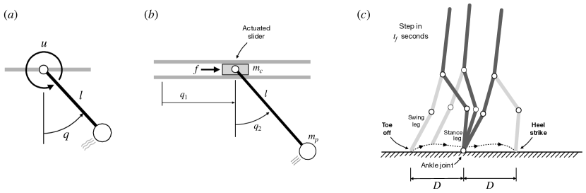
Figure 1: Test cases. (a) A simple actuated pendulum. (b) A cart-pole system that has to perform a swing-up motion. (c) A five-link biped walking under a periodic gait. The three snapshots on the right illustrate the motion that occurs between the toe off and heel strike events defining a period of the gait.

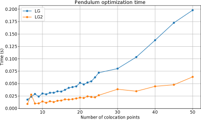
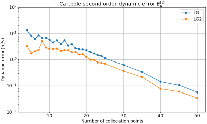
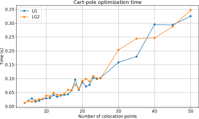
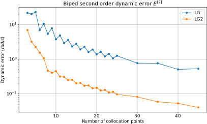
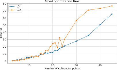
Figure 2: Second order dynamic error (left plots) and time used to solve the transcribed NLP problems (right) for an increasing number of collocation points in the three test cases considered. For the cartpole system, only the plot of $E_{q_{1}}^{[2]}$ is provided, as the one of $E_{q_{2}}^{[2]}$ shows a similar trend.

The first and second order versions of the Legendre-Gauss method are next compared in terms of performance, by applying them to solve the pendulum swing-up problem and two trajectory optimization problems thoroughly documented in [11], namely, the cart-pole swing-up and the five-link bipedal walking problems (Fig. 1). Analytical solutions for these problems are rather complex or directly not available, so in order to compare the methods, we compute the dynamic transcription error produced by each of them. To this end, we define the following errors.

The first order dynamic error of the $q_{i}$ coordinate is

$$\varepsilon^{[1]}_{q_{i}}(t)=\dot{q}_{i}(t)-v_{i}(t).$$ (17)

In general, this error is non-null in the first order LG method, as it does not enforce $v_{i}(t)=\dot{q}_{i}(t)$ for all $t$. However, it becomes zero by definition when using the second order method. For the same coordinate, the second order dynamic error is

$$\varepsilon^{[2]}_{q_{i}}(t)=\ddot{q}_{i}(t)-g_{i}({\mbox{\bm{$q$}}},{\mbox{\bm{$\dot{q}$}}},{\mbox{\bm{$u$}}},t).$$ (18)

We found the 2 order error more meaningful than the 1 order error reported in [11], since it reflects the deviation from the actual system dynamics, which is expected to be minimized by the collocation process. When all coordinates in $q$ have the same units, it also makes sense to define a joint error for all coordinates. A plausible definition for this error is

$$\varepsilon^{[2]}(t)=|\varepsilon^{[2]}_{q_{1}}(t)|+\ldots+|\varepsilon^{[2]}_{q_{n_{q}}}(t)|.$$ (19)

Finally, to summarize the error functions in just one number, we compute their integrals over $[0,t_{f}]$:

$$E^{[r]}_{q_{i}} =\int_{0}^{t_{f}}|\varepsilon^{[r]}_{q_{i}}(t)|\;dt, r=1,2,$$ (20)

$$E^{[r]} =\int_{0}^{t_{f}}\varepsilon^{[r]}(t)\;dt, r=1,2.$$ (21)

To perform the comparisons, we have implemented the methods in Python using the symbolic package SymPy [12] to model the systems, and the toolbox CasADi [13] to solve the NLP problems that result. CasADi provides the necessary means to formulate such problems and to compute the gradients and Hessians of the transcribed equations using automatic differentiation. These are necessary to solve the NLP problems, a task for which we rely on the interior-point solver IPOPT [14] in conjunction with the linear solver MUMPS [15]. The execution times we report have been obtained on a single-thread implementation running on an iMac computer with an Intel i7, 8-core 10th generation processor at 3.8 GHz.

In what follows, and in order to simplify the explanations, we use the shorthands LG and LG2, respectively, for the first and second order versions of the Legendre-Gauss pseudospectral methods. Fig. 2 provides a comparison of the second order errors and optimization times for both methods in all problems, showing mean results after 10 runs.

V-A The pendulum swing-up problem

The system consists of a pendulum formed by a single link connected to ground with a revolute joint (Fig. 1(a)). The angle of the pendulum relative to the rest position is given by $q$ and the revolute joint is powered by a motor, which applies a torque $u$ to the link. Starting with the pendulum hanging at rest in its bottom position, the goal is to reach the upright configuration with zero velocity in the shortest possible time $t_{f}$. The cost functional to be minimized is

$$J(u(t))=\int_{0}^{t_{f}}dt=t_{f}.$$ (22)

From the top plots in Fig. 2 we observe that the use of LG2 reduces both the second order dynamic error and the computation time. The error is reduced in about two orders of magnitude, with the gain increasing with $N$, while the optimization time is approximately halved for all $N$.

V-B The cart-pole swing-up problem

The cart-pole system comprises a cart that travels along a horizontal track and a pendulum that hangs freely from the cart (Fig. 1(b)). A motor drives the cart forward and backward along the track. Starting with the pendulum hanging below the cart at rest at a given position, the goal is to reach a final configuration in a given time $t_{f}$, with the pendulum stabilized at a point of inverted balance and the cart staying at rest at a distance $d$ from the initial position. The cost functional to be minimized is

$$J(u(t))=\int_{0}^{t_{f}}u^{2}(t)dt,$$ (23)

where $u$ is the force applied to the cart, and we adopt the same dynamic equations and problem parameters as in [11].

It can be observed in the middle row of Fig. 2 that the use of the second order method reduces the second order dynamic error in about 40% for all values of $N$ (left plot), while using a similar computation time in both methods (right plot).

V-C The 5-link bipedal walking problem

We next apply the methods to optimize a periodic gait for the planar biped robot shown in Fig. 1(c). The robot involves five links pairwise connected with revolute joints, forming two legs and a torso. All joints are powered by torque motors, with the exception of the ankle joint, which is passive. Like the cart pole system, therefore, this robot is underactuated, but it is substantially more complex. The system is commonly used as a testbed when studying bipedal walking [16, 17, 18, 19].

For this example we use the dynamic model given in [11], which matches the one in [16] with parameters corresponding to the RABBIT prototype [20]. We assume the robot is left-right symmetric, so we can search for a periodic gait using a single step, as opposed to a stride, which involves two steps. This means that the state and torque trajectories will be the same on each successive step.

As in [11], we define $q$ as the vector that contains the absolute angles of all links relative to ground, while $u$ encompasses all motor torques. Also as in [11], and similarly to the cart-pole problem, our goal is to find state and action trajectories ${\mbox{\bm{$x$}}}(t)$ and ${\mbox{\bm{$u$}}}(t)$ that define an optimal gait under the cost

$$J({\mbox{\bm{$u$}}}(t))=\int_{0}^{t_{f}}{\mbox{\bm{$u$}}}(t)^{\mathsf{T}}{\mbox{\bm{$u$}}}(t)\;dt.$$ (24)

For this problem, the bottom row of Fig. 2 shows that our modified second order LG method results in a reduction of the second order dynamic error. Such a reduction increases with $N$ until about $N=8$, and stabilizes at about one order of magnitude from then on. However, we can observe that this comes at the cost of increasing the optimization time a bit (by a factor of at most 2 in the worst cases) for values of $N$ above $15$.

VI Conclusions

This paper has presented a modified version of the LG pseudospectral method that is able to correctly deal with the second order nature of the dynamical systems frequently arising in robotics. In comparison to the classical LG method, the one we present guarantees that the approximation polynomials for the velocity are the time derivative of the polynomials for the configuration, which results in trajectories which are more in agreement with the system dynamics. The use of an additional node point in the definition of the configuration polynomials, moreover, has allowed us to have $N+2$ independent parameters for each component of the configuration vector. When stating an initial state and control trajectory, two initial value constraints and $N$ collocation constraints were defined for each component, all of them independent, therefore retaining the ability of the usual LG method to solve initial value problems. Using three benchmark problems from the literature, moreover, we have shown that the new LG method provides trajectories with a much smaller dynamic error in comparison to the usual LG method. This implies that the obtained trajectories will be more compliant with the system dynamics, which should facilitate their tracking control in practice.

Points that deserve further attention include the study of problem characteristics that lead to an increase or decrease of the computing time when switching the methods, the application of the new formulation to finite element methods that use several polynomials in sequence, instead of a single global polynomial, and a detailed theoretical analysis of the second order LG method to confirm that the usual good properties of LG methods, which include symplecticity, symmetry, and the smallest possible global error for a polynomial of a given degree [21], are preserved.

References

- [1] Y. Zhao, H.-C. Lin, and M. Tomizuka, “Efficient Trajectory Optimization for Robot Motion Planning,” in 2018 15th International Conference on Control, Automation, Robotics and Vision (ICARCV), 2018, pp. 260–265.
- [2] A. Hereid, S. Kolathaya, and A. D. Ames, “Online optimal gait generation for bipedal walking robots using Legendre pseudospectral optimization,” in 2016 IEEE 55th Conference on Decision and Control (CDC). IEEE, 2016, pp. 6173–6179.
- [3] A. Patel, S. L. Shield, S. Kazi, A. M. Johnson, and L. T. Biegler, “Contact-implicit trajectory optimization using orthogonal collocation,” IEEE Robotics and Automation Letters, vol. 4, no. 2, pp. 2242–2249, 2019.
- [4] N. Bedrossian, S. Bhatt, M. Lammers, L. Nguyen, and Y. Zhang, “First Ever Flight Demonstration of Zero Propellant Maneuver (TM) Attitute Control Concept,” in AIAA Guidance, Navigation and Control Conference and Exhibit, 2007.
- [5] I. M. Ross and M. Karpenko, “A review of pseudospectral optimal control: From theory to flight,” Annual Reviews in Control, vol. 36, no. 2, pp. 182–197, 2012.
- [6] G. N. Elnagar and M. A. Kazemi, “Pseudospectral Chebyshev Optimal Control of Constrained Nonlinear Dynamical Systems,” Computational Optimization and Applications, vol. 11, no. 2, pp. 195–217, 1998.
- [7] D. Garg, M. Patterson, W. W. Hager, A. V. Rao, D. A. Benson, and G. T. Huntington, “A unified framework for the numerical solution of optimal control problems using pseudospectral methods,” Automatica, vol. 46, no. 11, pp. 1843–1851, 2010.
- [8] R. Tedrake, Underactuated Robotics: Algorithms for Walking, Running, Swimming, Flying, and Manipulation., 2022, course notes for MIT 6.832, downloaded on 29 July 2022.
- [9] I. M. Ross, J. Rea, and F. Fahroo, “Exploiting higher-order derivatives in computational optimal control,” in Proc. of the 10th Mediterranean Conference on Control and Automation (MED2002), 2002.
- [10] S. Moreno-Martin, L. Ros, and E. Celaya, “Collocation Methods for Second Order Systems,” in Proceedings of Robotics: Science and Systems, New York City, NY, USA, June 2022.
- [11] M. Kelly, “An Introduction to Trajectory Optimization: How to Do Your Own Direct Collocation,” SIAM Review, vol. 59, no. 4, pp. 849–904, 2017.
- [12] A. Meurer, C. P. Smith, M. Paprocki, O. Čertík, S. B. Kirpichev, M. Rocklin, A. Kumar, S. Ivanov, J. K. Moore, S. Singh, T. Rathnayake, S. Vig, B. E. Granger, R. P. Muller, F. Bonazzi, H. Gupta, S. Vats, F. Johansson, F. Pedregosa, M. J. Curry, A. R. Terrel, v. Roučka, A. Saboo, I. Fernando, S. Kulal, R. Cimrman, and A. Scopatz, “SymPy: symbolic computing in Python,” PeerJ Computer Science, vol. 3, p. e103, Jan. 2017.
- [13] J. A. E. Andersson, J. Gillis, G. Horn, J. B. Rawlings, and M. Diehl, “CasADi – A software framework for nonlinear optimization and optimal control,” Mathematical Programming Computation, vol. 11, no. 1, pp. 1–36, 2019.
- [14] A. Wächter and L. T. Biegler, “On the implementation of an interior-point filter line-search algorithm for large-scale nonlinear programming,” Mathematical programming, vol. 106, no. 1, pp. 25–57, 2006.
- [15] P. R. Amestoy, I. S. Duff, J.-Y. L’Excellent, and J. Koster, “A Fully Asynchronous Multifrontal Solver Using Distributed Dynamic Scheduling,” SIAM Journal on Matrix Analysis and Applications, vol. 23, no. 1, pp. 15–41, 2001.
- [16] E. R. Westervelt, J. W. Grizzle, and D. E. Koditschek, “Hybrid zero dynamics of planar biped walkers,” IEEE Transactions on Automatic Control, vol. 48, no. 1, pp. 42–56, 2003.
- [17] T. Yang, E. R. Westervelt, A. Serrani, and J. P. Schmiedeler, “A framework for the control of stable aperiodic walking in underactuated planar bipeds,” Autonomous Robots, vol. 27, no. 3, pp. 277–290, 2009.
- [18] H.-W. Park, K. Sreenath, A. Ramezani, and J. W. Grizzle, “Switching control design for accommodating large step-down disturbances in bipedal robot walking,” in 2012 IEEE International Conference on Robotics and Automation. IEEE, 2012, pp. 45–50.
- [19] C. O. Saglam and K. Byl, “Robust Policies via Meshing for Metastable Rough Terrain Walking.” in Robotics: Science and Systems, 2014.
- [20] C. Chevallereau, G. Abba, Y. Aoustin, F. Plestan, E. Westervelt, C. C. De Wit, and J. Grizzle, “RABBIT: a testbed for advanced control theory,” IEEE Control Systems Magazine, vol. 23, no. 5, pp. 57–79, 2003.
- [21] E. Hairer, C. Lubich, and G. Wanner, Geometric numerical integration: structure-preserving algorithms for ordinary differential equations. Springer, 2006.