Normalized Random Meaures with Interacting Atoms for Bayesian Nonparametric Mixtures

Abstract

The study of almost surely discrete random probability measures is an active line of research in Bayesian nonparametrics. The idea of assuming interaction across the atoms of the random probability measure has recently spurred significant interest in the context of Bayesian mixture models. This allows the definition of priors that encourage well separated and interpretable clusters. In this work, we provide a unified framework for the construction and the Bayesian analysis of random probability measures with interacting atoms, encompassing both repulsive and attractive behaviors. Specifically we derive closed-form expressions for the posterior distribution, the marginal and predictive distributions, which were not previously available except for the case of measures with i.i.d. atoms. We show how these quantities are fundamental both for prior elicitation and to develop new posterior simulation algorithms for hierarchical mixture models. Our results are obtained without any assumption on the finite point process that governs the atoms of the random measure. Their proofs rely on new analytical tools borrowed from the theory of Palm calculus and that might be of independent interest. We specialize our treatment to the classes of Poisson, Gibbs, and Determinantal point processes, as well as to the case of shot-noise Cox processes.

Keywords: Distribution theory, Posterior distribution, Prediction, Repulsive point processes, Palm calculus.

1 Introduction

Random measures provide one of the main building blocks of Bayesian nonparametric (BNP) inference, where they are used to directly model the observational process as, e.g., in species sampling or feature sampling problems, or a latent unobserved process as in mixture models. In particular, mixtures are powerful tools to perform model-based clustering. Nevertheless, it is common folklore that traditional BNP mixture models have a major drawback in that the cluster estimate is not robust to model misspecification; see Cai et al. (2021) and Guha et al. (2021). Repulsive mixture models (Petralia et al., 2012; Beraha et al., 2022; Bianchini et al., 2020; Quinlan et al., 2020; Xie and Xu, 2019; Xu et al., 2016) offer a solution to this problem. Despite their recent popularity, mathematical properties of repulsive mixtures have not been thoroughly investigated so far. In this paper, we provide a general framework for mixture models encompassing repulsiveness as well as other forms of dependence in the locations, such as attractiveness. In particular, we fill a gap in the literature by providing a unified framework allowing for the analysis of the associated mixing measure and establish general results characterizing the distribution (both a priori and a posteriori) of several functionals of interest. Our results do not merely generalize existing theory, but they shed light on large classes of processes which are used in applications without appropriate theoretical investigation. Our methodology can also be exploited to devise new computational procedures, never explored in the existing literature, such as marginal algorithms. As a further original contribution, the proofs of the main theorems are interesting per se, since they include new technical tools, mainly based on Palm calculus.

1.1 Almost surely discrete random probability measures

We focus on almost surely discrete random measures of the form $\tilde{p}=\sum_{j\geq 1}p_{j}\delta_{X_{j}}$, whose total mass is almost surely equal to one, i.e., on random probability measures (RPMs). From the seminal work of Ferguson (Ferguson, 1973) on the Dirichlet process, a variety of approaches for the construction of RPMs have been introduced. A fruitful strategy is based on the normalization of completely random measures with infinite activity, i.e., whose number of support points $(X_{j})_{j\geq 1}$ is countably infinite. This idea, systematically introduced in Regazzini et al. (2003) for measures on $\mathbb{R}$ with the name of normalized random measures with independent increments (NRMI), has been extended later to more general spaces (see, e.g., James et al., 2009). More recently, Argiento and De Iorio (2022) have exploited the same ideas to construct random probability measures with a random finite number of support points, named normalized independent finite point processes. Both approaches build a discrete RPM by normalizing a marked point process where the points of the process define the jumps $(p_{j})_{j\geq 1}$ of the RPM and i.i.d. marks $(X_{j})_{j\geq 1}$ define the atoms. See also Lijoi et al. (2022) for an allied approach.

As one of the main contributions in this paper, we propose a construction of RPMs via normalization of marked point processes with inverted roles with respect to Regazzini et al. (2003) and Argiento and De Iorio (2022). In our construction, indeed, the atoms $(X_{j})_{j\geq 1}$ are the points of a general simple point process, while the weights $(p_{j})_{j\geq 1}$ are obtained by normalizing i.i.d. positive marks associated with the atoms. Through the law of the point process, we are able to encourage different behaviors among the support points of the random probability measure, such as independence (when the point process is Poisson or the class of independent finite point processes), separation (i.e., the support points are well separated, when the point process is repulsive, such as Gibbs or determinantal point processes), and also random aggregation (i.e., the support points are clustered together, when the point process is of Cox type). As special cases, our construction recovers the mixing measures used in the repulsive mixture models in the literature so far, where the repulsion is on the locations, and also the mixture of mixtures prior in Malsiner-Walli et al. (2017).

1.2 Overview and outline

In the context of mixture models, the RPM $\tilde{p}$ is the mixing measure of the mixture model and data are generated from the mixture of a parametric density. The mixture model can be equivalently assigned as

$$Z_{i}\,|\,Y_{i}\stackrel{{\scriptstyle\mbox{\scriptsize ind}}}{{\sim}}f(\cdot\,|\,Y_{i}),\qquad Y_{i}\,|\,\tilde{p}\stackrel{{\scriptstyle\mbox{\scriptsize iid}}}{{\sim}}\tilde{p},\qquad i=1,\ldots,n,$$

where $f(\cdot\,|\,Y)$ is a suitable parametric density function. A fundamental preliminary step for Bayesian inference in the mixture model is to study the distributional properties of the latent sample $Y_{1},\ldots,Y_{n}$. Specifically, for prior elicitation purposes, it is interesting to investigate the moments of $\tilde{p}$, the prior distribution of the distinct values in the sample, and the marginal distribution of the $Y_{i}$’s. For inferential purposes instead, both from a methodological and computational perspective, it is central to derive the conditional distribution of $\tilde{p}$ given $Y_{1},\ldots,Y_{n}$, as well as the predictive distribution of $Y_{n+1}$ given the latent sample.

In this paper, we provide general closed-form expressions for all these quantities for any choice of the point process distribution, allowing for a universal theory of very different dependence behaviour such as repulsion or attractiveness. These are the counterpart of well-known results for NRMIs. Though these expressions are, in general, difficult to evaluate, they drastically simplify in the case of well-known point processes such as the Poisson, the Gibbs or the determinantal point processes. We also consider a new case of cluster process mixtures, using the shot-noise Cox process as the distribution of the atoms $(X_{j})_{j\geq 1}$, which is rather new in this type of literature. This class of point processes exhibits random aggregation structure, and we suggest that this might be useful in the context of mixture models to perform clustering when the model is misspecified.

From the technical point of view, our results are based on an application of Palm calculus, a fundamental tool in studying point processes. In the context of BNP models, Palm calculus was introduced in James (2002, 2005) for the analysis of random probability measures built from Poisson processes. See also James (2006) and James et al. (2009) for applications to the Bayesian analysis of neutral to the right processes and mixtures of normalized completely random measures, respectively. Essentially, Palm calculus can be regarded as an extension of Fubini’s theorem. It allows to exchange the expectation and integral signs when both are with respect to a point process, with the subtle difference that (in general) the expectation is now taken with respect to the law of another point process, i.e., the reduced Palm version of the original process. In the Poisson process case (and therefore in the case of completely random measures), the reduced Palm version coincides with the law of the original Poisson process, for which computations are usually easy. This property characterizes Poisson processes (Last and Penrose, 2017).

When considering random measures built from general point processes, the results in James (2002) do not apply, since the reduced Palm version does not have the self-similarity property of the Poisson process. Hence, while our results are similar in the spirit of James et al. (2009), the associated technical tools used are substantially different.

The rest of the paper is structured as follows. Section 2 introduces the model for the $Y_{i}$’s and the general construction for normalized random measures based on marked point processes, and gives preliminaries on Palm calculus, a basic tool needed for all our proofs. In Section 3 we analyse the properties of the prior distribution of our random measures. The posterior distribution of the random measure, the marginal distribution of the $Y_{i}$’s, the prior distribution of the distinct values in the latent sample, and the predictive distribution of a new observation are presented in Section 4. In Section 5 we show how to construct Bayesian mixture models based on our class of random probability measures, which act as the mixing measure of the mixture model. We discuss two Markov chain Monte Carlo algorithms to approximate the posterior distribution. Section 6 focuses on the class of shot-noise Cox process (Møller, 2003) and its use in mixture models. Proofs and analytical details of the examples are deferred to the Appendix.

2 Model definition and preliminaries

We consider a sequence of random variables $(Y_{i})_{i\geq 1}$ defined on the probability space $(\Omega,\mathcal{A},\mathsf{P})$ and taking values in the Polish space $(\mathbb{X},\mathcal{X})$, endowed with its Borel $\sigma$-algebra. Moreover, we denote by $\mathbb{P}(\mathbb{X})$ the space of all probability measures over $(\mathbb{X},\mathcal{X})$, and $\mathcal{P}(\mathbb{X})$ stands for the corresponding Borel $\sigma$-algebra. We also indicate by $\bm{Y}:=(Y_{1},\ldots,Y_{n})$ the sample of size $n$, with $n\geq 1$. Note that, in this and in the following two sections, $\bm{Y}$ represents the data points. We suppose that

$$Y_{i}\,|\,\tilde{p} \stackrel{{\scriptstyle\mbox{\scriptsize iid}}}{{\sim}}\tilde{p}\quad i\geq 1$$ (1)

$$\tilde{p} \sim Q,$$

where $Q$ is a distribution over $\left(\mathbb{P}(\mathbb{X}),\mathcal{P}(\mathbb{X})\right)$. Note that, by the de Finetti’s theorem (de Finetti, 1937), (1) is equivalent to assuming that the $Y_{i}$’s are exchangeable, which justifies the Bayesian approach to inference.

2.1 Random measures as functionals of point processes

We start by basic definitions. Let $\mathbb{M}(\mathbb{X})$ be the space of locally finite measures on $\mathbb{X}$ and denote by $\mathcal{M}(\mathbb{X})$ its Borel $\sigma$-algebra. A (simple) point process $\Phi$ on $\mathbb{X}$ is a random measure with values in $\mathbb{M}(\mathbb{X})$ defined as

$$\Phi(B)=\sum_{j\geq 1}\delta_{X_{j}}(B),\qquad B\in\mathcal{X},$$ (2)

where $(X_{j})_{j\geq 1}$, named points of the process, is a random countable subset of $\mathbb{X}$ such that $\mathsf{P}(X_{i}=X_{j})=0$ for all $i\neq j$. We denote by $\mathbf{P}_{\Phi}$ the distribution of $\Phi$, that is $\mathbf{P}_{\Phi}(L)=\mathsf{P}(\Phi\in L)$ for any $L\in\mathcal{M}(\mathbb{X})$. In the rest of the paper, we deliberately confuse the points of the process $\Phi$ and the random measure associated to $\Phi$. In this work, we follow notation as in Baccelli et al. (2020); see this reference for more details on point processes. If, for $A_{1},\ldots,A_{n}\in\mathcal{X}$ disjoint sets and for any $n\geq 1$, the random elements $\Phi(A_{1}),\ldots,\Phi(A_{n})$ are independent Poisson random variables with parameters $\omega(A_{1}),\ldots,\omega(A_{n})$, respectively, where $\omega$ is a locally finite measure on $\mathbb{X}$, the point process $\Phi$ in (2) is a Poisson process with mean measure $\omega$, or, alternatively, with intensity $\omega(dx)$. We use notation $\Phi\sim{\rm PP}(\omega)$. The Poisson point process can also be used as reference measure on $(\mathbb{M}_{\mathbb{X}},\mathcal{M}_{\mathbb{X}})$ to define the law of other point processes by specifying their Radon-Nikodym density. Formally, let $\tilde{N}$ be a Poisson point process on $(\mathbb{X},\mathcal{X})$ with distribution $\mathbf{P}_{N}$; a point process $\Phi$ on $(\mathbb{X},\mathcal{X})$ is absolutely continuous with respect to $\tilde{N}$ if for any $L\in\mathcal{M}(\mathbb{X})$ such that $\mathsf{P}(\tilde{N}\in L)=0$, one has $\mathsf{P}(\Phi\in L)=0$. The Radon-Nikodym theorem yields the existence of the density $f_{\Phi}:\mathbb{X}\rightarrow\mathbb{R}_{+}$ (i.e., the Radon-Nikodym derivative) such that

$$\mathbf{P}_{\Phi}(\mathrm{d}\nu)=f_{\Phi}(\nu)\mathbf{P}_{N}(\mathrm{d}\nu).$$ (3)

A marked point process is such that $\Phi=\sum_{j\geq 1}\delta_{(X_{j},S_{j})}$, where $(X_{j})_{\geq 1}$ is a countable subset of $\mathbb{X}$ and $(S_{j})_{j\geq 1}$, denoted as marks, are a sequence of independent random variables such that the distribution of any $S_{j}$ might depend only on the corresponding marked r.v. $X_{j}$.

By independent finite point process (IFPP) we mean a point process $\Phi$ such that $(X_{j})_{j\geq 1}=(X_{1},\ldots,X_{M})$, where $M$ is a discrete r.v. and $X_{1},\ldots,X_{M}$, conditionally to $M$, are independent identically distributed (i.i.d.) random variables.

A purely atomic (with no fixed points) completely random measure (CRM) is defined (see Kingman, 1992) as

$$\tilde{\mu}(B):=\int_{\mathbb{R}_{+}\times B}s\tilde{N}(\mathrm{d}s\,\mathrm{d}x)=\sum_{j\geq 1}S_{j}\delta_{X_{j}}(B),\qquad B\in\mathcal{X}$$ (4)

where $\tilde{N}=\sum_{j\geq 1}\delta_{(S_{j},X_{j})}$ is a Poisson process on $\mathbb{R}^{+}\times\mathbb{X}$ with mean measure $\omega$. For any collection of disjoint measurable sets $A_{1},\ldots,A_{n}\in\mathcal{X}$ and for any $n\geq 1$, the r.v.’s $\tilde{\mu}(A_{1}),\ldots,\tilde{\mu}(A_{n})$ are independent. The typical assumption is that the CRM $\tilde{\mu}$ is homogeneous, i.e., $\omega(\mathrm{d}s\,\mathrm{d}x)=\nu(s)\mathrm{d}s\,G_{0}(\mathrm{d}x)$, $\nu(s)$ being the density of a non-negative measure on $\mathbb{R}^{+}$ and $G_{0}$ being a diffuse probability on $\mathbb{X}$. Since $\tilde{\mu}$ is homogeneous, the support points $\left(X_{j}\right)_{j\geq 1}$ and the jumps $\left(S_{j}\right)_{j\geq 1}$ of $\tilde{\mu}$ are independent, moreover the $X_{j}$’s are independent identically distributed random variables from $G_{0}$, while $\left(S_{j}\right)_{j\geq 1}$ are the points of a Poisson process on $\mathbb{R}^{+}$ with mean intensity $\nu$.

A random probability measure $\tilde{p}$ can be defined through normalization of $\tilde{\mu}$ as

$$\tilde{p}(\cdot)=\sum_{j\geq 1}\frac{S_{j}}{\tilde{\mu}(\mathbb{X})}\delta_{X_{j}}(\cdot)$$ (5)

provided that $\mathsf{P}(0<\tilde{\mu}(\mathbb{X})<+\infty)=1$. See Regazzini et al. (2003). As an alternative approach, Argiento and De Iorio (2022) build an almost surely discrete RPM with weights obtained by normalization of a finite point process. Their construction is similar to the definition of normalized CRMs given in (5); they start from (4) substituting the Poisson process $\tilde{N}$ with points $(S_{j},X_{j})_{j\geq 1}$ by an IFPP such that $(S_{j})_{j=1}^{M}$ and $(X_{j})_{j=1}^{M}$ are independent. Alternatively, the construction of both normalized CRM’s and normalized IFPP can be unified starting from (4), interpreting $\tilde{N}$ as a marked point process. In particular, the unnormalized weights $(S_{j})_{j\geq 1}$ are the points of a point process on $\mathbb{R}_{+}$, marked with i.i.d. random atoms $(X_{j})_{j\geq 1}$ in $\mathbb{X}$.

In this work, we consider the exchangeable framework (1) and propose a general construction for the random probability measure $\tilde{p}$, termed normalized random measure (nRM) that is based on general point processes other than the Poisson or IFPP cases. In particular, we revert the roles of the $S_{j}$’s and the $X_{j}$’s in the construction of the marked point process to define (5): we assume that the atoms $(X_{j})_{j\geq 1}$ are the points of a point process, marked with the unnormalized weights $(S_{j})_{j\geq 1}$. This allows the construction of repulsive or attractive location mixtures, which necessarily imply mixing measures $\tilde{p}$’s with non i.i.d. atoms.

To build a nRM, let $\Phi=\sum_{j\geq 1}\delta_{X_{j}}$ be a point process with points in $\mathbb{X}$ having distribution $\mathbf{P}_{\Phi}$. Then, we consider the marked point process $\Psi$ on $\mathbb{X}\times\mathbb{R}_{+}$, $\Psi=\sum_{j\geq 1}\delta_{(X_{j},S_{j})}$, constructed by assigning to the points in $\Phi$ i.i.d. marks $S_{j}$’s with marginal distribution $H$ on the positive real line. Now define a random measure $\tilde{\mu}$ from $\Psi$ as follows

$$\tilde{\mu}(B)=\int_{B\times\mathbb{R}_{+}}s\Psi(\mathrm{d}x\,\mathrm{d}s)=\sum_{j\geq 1}S_{j}\delta_{X_{j}}(B),\qquad B\in\mathcal{X}.$$ (6)

Note that, when $\Phi$ is a Poisson point process, we recover the construction of a completely random measure, while when $\Phi$ is a IFPP, we get the RPM defined in Argiento and De Iorio (2022).

To define $\tilde{p}$ though normalization, first we assume that $\Phi$ in (6) is a finite point process, so that $\tilde{\mu}(\mathbb{X})<+\infty$ a.s.. We adopt this condition in the rest of the paper. Instead of assuming $\tilde{\mu}(\mathbb{X})>0$ a.s., we set $\tilde{\mu}/\tilde{\mu}(\mathbb{X})\equiv 0$ any time that $\tilde{\mu}(\mathbb{X})=0$. In the latter case, we intend that the model does not generate any observation $Y_{i}$. A similar agreement is adopted in Zhou et al. (2017). If we do observe datapoints, then $\mathsf{P}(\tilde{\mu}(\mathbb{X})=0\,|\,Y_{1},\ldots,Y_{n})=0$, as shown in Theorem 4.1 below. Hence, a posteriori, the usual assumption $\tilde{\mu}(\mathbb{X})>0$ a.s. is guaranteed. Consequently $\tilde{p}:=\tilde{\mu}/\tilde{\mu}(\mathbb{X})$, where $\tilde{\mu}$ is as in (6), is well defined and has the same representation as in (5). We write $\tilde{p}\sim{\rm nRM}(\mathbf{P}_{\Phi},H)$ to denote the distribution of the normalized random measure, while $\tilde{\mu}\sim{\rm RM}(\mathbf{P}_{\Phi},H)$ stands for the distribution of the associated unnormalized random measure. With a little abuse of notation we will also denote by $\mathbf{P}_{\Psi}$ the law of $\tilde{\mu}$, where $\Psi$ is $\Phi$ with marks from $H$. Note that, as it is clear from the definition, $\tilde{p}\sim\mbox{nRM}(\mathbf{P}_{\Phi},H)$ does not lie in the class of species sampling models (Pitman, 1996), since, for instance, the support points are not i.i.d..

For the sake of concreteness, beside Poisson processes, we illustrate two important examples of point processes $\Phi$ such as Gibbs and determinantal point processes. These particular specifications allow for explicit expressions of relevant functionals of the prior and posterior of $\tilde{p}$ and of its associated mixture model.

Example 2.1 (Gibbs point processes).

Following Baccelli et al. (2020), the probability distribution of a Gibbs type point process has a density $f_{\Phi}$ with respect to the law of a Poisson point process $\tilde{N}$ as in (3). In the following, we always consider densities with respect to the unit-intensity Poisson point process on a compact subset $R$, that is, $\tilde{N}$ has intensity $\omega(dx)=\mathbbm{1}_{R}(dx)$.

In practice, we assign a Gibbs point process through its density $f_{\Phi}$. However, this task might be complex because of the constraint $\mathsf{E}[f_{\Phi}(\tilde{N})]=1$. In particular, the expected value cannot be computed in closed form even for very simple densities, to the best of our knowledge. Therefore, unnormalized densities $g_{\Phi}$ such that $\mathsf{E}[g_{\Phi}(\tilde{N})]<+\infty$ are typically considered and then normalized as $f_{\Phi}(\nu)=g_{\Phi}/Z$, where $Z:=\mathsf{E}[g_{\Phi}(\tilde{N})]$ are intractable normalizing constants. Among the other Gibbs points processes, we mention the Strauss process (see Beraha et al., 2022, Section 2.1). See also Møller and Waagepetersen (2003) for different examples of Gibbs point processes and associated unnormalized densities.

We assume that $\Phi$ is hereditary, meaning that for any $\nu=\sum_{j=1}^{m}\delta_{X_{j}}\in\mathbb{M}(\mathbb{X})$ and $X^{*}\in\mathbb{X}\setminus\{X_{1},\ldots X_{m}\},$ $g_{\Phi}(\nu+\delta_{X^{*}})>0$ implies $g_{\Phi}(\nu)>0$. Then we can introduce the Papangelou conditional intensity defined as

$$\lambda_{\Phi}(\nu;\bm{X}^{*})=\frac{f_{\Phi}\left(\nu+\sum_{j=1}^{k}\delta_{X^{*}_{j}}\right)}{f_{\Phi}\left(\sum_{j=1}^{k}\delta_{X^{*}_{j}}\right)}=\frac{g_{\Phi}\left(\nu+\sum_{j=1}^{k}\delta_{X^{*}_{j}}\right)}{g_{\Phi}\left(\sum_{j=1}^{k}\delta_{X^{*}_{j}}\right)}$$ (7)

where $\bm{X}^{*}=\{X^{*}_{1},\ldots,X^{*}_{k}\}$. The Papangelou conditional intensity can be understood as the conditional “density” of $\Phi$ having atoms as in $\nu$, given that the rest of $\Phi$ is $\bm{X}^{*}$. We say that a Gibbs point process $\Phi$ has a repulsive behavior if $\lambda_{\Phi}(\nu;\bm{X}^{*})$ is a nonincreasing function of $\bm{X}^{*}$, that is, $\lambda_{\Phi}(\nu;\bm{X}^{*})\geq\lambda_{\Phi}(\nu;\bm{X}^{*}\cup X^{\prime})$ for any $X^{\prime}\in\mathbb{X}\setminus(\bm{X}^{*}\cup X^{\prime})$.

When Gibbs point processes are used as mixing measures in Bayesian mixture models, posterior inference is not affected by the normalizing constant $Z$ if the hyper-parameters appearing in the density $g_{\Phi}$ are fixed. In the opposite case, updating those hyper-parameters is a “doubly intractable” problem. See, e.g., Beraha et al. (2022) for a solution. Nevertheless, in the rest of the paper, we consider these hyper-parameters as fixed.

Example 2.2 (Determinantal point processes).

Determinantal point processes (DPPs Macchi, 1975; Hough et al., 2009; Lavancier et al., 2015) are a class of repulsive point processes. We will restrict our focus to finite DPPs defined on a compact region $R\subset\mathbb{X}=:\mathbb{R}^{q}$. Consider a complex-valued covariance function $K:R\times R\to\mathbb{C}$ with spectral representation

$$K(x,y)=\sum_{h\geq 1}\lambda_{h}\varphi_{h}(x)\overline{\varphi_{h}(y)},\qquad x,y\in R$$ (8)

where $(\varphi_{h})_{h\geq 1}$ for an orthonormal basis for $L^{2}(R)$, $\lambda_{h}\geq 0$ with $\sum_{h\geq 1}\lambda_{h}<+\infty$. The general construction of a DPP is given by introducing independent Bernoulli variables $B_{h}\sim\mbox{Bern}(\lambda_{h})$ and considering $K^{\prime}(x,y)=\sum_{h\geq 1}B_{h}\varphi_{h}(x)\overline{\varphi_{h}(y)}$. Then, conditional on $(B_{h})_{h\geq 1}$, a DPP $\Phi$ with kernel $K$ has density with respect to the unit-intensity Poisson point process on $R$ given by

$$f_{\Phi\,|\,(B_{h})_{h}}(\nu)\propto\det\left\{K^{\prime}(x,y)\right\}_{x,y\in\nu},$$

where $\left\{K^{\prime}(x,y)\right\}_{x,y\in\nu}$ is the $n_{\nu}\times n_{\nu}$ matrix with entries $K^{\prime}(x,y)$, $x,y\in\nu$, and $n_{\nu}$ is the cardinality of $\nu$. We remark that $\Phi$ consists of exactly $\sum_{h\geq 1}B_{h}$ points almost surely. The existence of a DPP with kernel $K$ is equivalent to $\lambda_{h}\leq 1$ for any $h\geq 1$; see Macchi (1975).

If one specializes the construction above to the case $\lambda_{h}<1$, it can be shown (cf.  Lavancier et al. (2015)) that a DPP has density $f_{\Phi}$ with respect to the unit-intensity Poisson process given by

$$f_{\Phi}(\nu)={\rm e}^{|R|-D}\det\left\{C(x,y)\right\}_{x,y\in\nu},$$

where $|\cdot|$ denotes the Lebesgue measure, $D:=-\sum_{h\geq 1}\log(1-\lambda_{h})$, and

$$C(x,y)=\sum_{h\geq 1}\frac{\lambda_{h}}{1-\lambda_{h}}\varphi_{h}(x)\overline{\varphi_{h}(y)},\qquad x,y\in R.$$

We conclude the section with elements of Palm calculus which is a fundamental tool to understand Bayesian analysis of nRM.

2.2 Palm distributions

Palm calculus is a basic tool in the study of point processes. For the analysis of random measures, the fundamental result from Palm theory is the Campbell-Little-Mecke formula, an extension of Fubini’s theorem, which allows to exchange expectation and integral when considering expressions involving the expectation of integrals of functionals of any point process $\Phi$, as

$$\mathsf{E}_{\Phi}\left[\int g(x,\Phi)\Phi(\mathrm{d}x)\right],\textrm{ for }g\geq 0.$$ (9)

In the expression above, the integral is with respect to the measure $\Phi$, and the expectation is with respect to the law of $\Phi$. For model (1), we see that the marginal distribution of the $Y_{i}$’s, the posterior distribution of $\tilde{\mu}$, as well as other important quantities such as the prior moments of $\tilde{\mu}$, can be expressed as or characterized by (9), where $\Phi$ is replaced by the marked point process $\Psi$ defined in (6). Hence, Palm calculus is the tool that we will use in all the proofs to derive our results. We provide background on Palm calculus in Appendix A and refer the interested reader to Kallenberg (1984); Coeurjolly et al. (2017); Baccelli et al. (2020) for a detailed account. In the following, we limit ourselves to introduce the Palm measure of a point process and provide some intuition around it.

For a point process $\Phi$ on $\mathbb{X}$, let us introduce the mean measure $M_{\Phi}$ as $M_{\Phi}(B):=\mathsf{E}[\Phi(B)]$ for all $B\in\mathcal{X}$. We define the Campbell measure $\mathcal{C}_{\phi}$ on $\mathbb{X}\times\mathbb{M}(\mathbb{X})$ as

$$\mathcal{C}_{\Phi}(B\times L)=\mathsf{E}\left[\Phi(B)\mathbbm{1}_{L}(\Phi)\right],\quad B\in\mathcal{X},L\in\mathcal{M}(\mathbb{X}).$$

Then, as a consequence of the Radon-Nikodym theorem, for any fixed $L$, there exists a $M_{\Phi}$-a.e. unique disintegration probability kernel $\{\mathbf{P}_{\Phi}^{x}(\cdot)\}_{x\in\mathbb{X}}$ of $\mathcal{C}_{\phi}$ with respect to $M_{\Phi}$, i.e.

$$\mathcal{C}_{\Phi}(B\times L)=\int_{B}\mathbf{P}_{\Phi}^{x}(L)M_{\Phi}(\mathrm{d}x)\quad B\in\mathcal{X},L\in\mathcal{M}(\mathbb{X}).$$

Note that, for any $x\in\mathbb{X}$, $\mathbf{P}_{\Phi}^{x}$ is the distribution of a random measure (specifically, a point process) on $\mathbb{X}$. See (Kallenberg, 2021, Theorem 31.1). Therefore, $\mathbf{P}_{\Phi}^{x}$ can be identified with the distribution of point process $\Phi_{x}$ such that $\mathbf{P}_{\Phi}^{x}(L)=\mathsf{P}(\Phi_{x}\in L)$. In particular, Proposition 3.1.12 in Baccelli et al. (2020) shows that the point process $\Phi_{x}$ has almost surely an atom at $x$. This property allows for the interpretation of $\mathbf{P}_{\Phi}^{x}$ as the probability distribution of the point process $\Phi$ given that (conditionally to) it has an atom at $x$. $\Phi_{x}$ is called the Palm version of $\Phi$ at $x$. Since $\delta_{x}$ is a fixed atom of $\Phi_{x}$, we subtract it from $\Phi_{x}$ and obtain the reduced Palm kernel, denoted by $\mathbf{P}_{\Phi^{!}}^{x}$, that is the law of the point process

$$\Phi^{!}_{x}:=\Phi_{x}-\delta_{x}.$$

The argument outlined above can be extended to the case of multiple points $\bm{x}=(x_{1},\ldots,x_{k})$, leading to the $k$-th Palm distribution $\{\mathbf{P}_{\Phi}^{\bm{x}}\}_{\bm{x}\in\mathbb{X}^{k}}$. Again, $\Phi_{\bm{x}}$ can be understood as the law of $\Phi$ conditional to $\Phi$ having atoms at $\{x_{1},\ldots,x_{k}\}$ and removing the trivial atoms yields the reduced Palm distribution that is the law of

$$\Phi^{!}_{\bm{x}}:=\Phi_{\bm{x}}-\sum_{j=1}^{k}\delta_{x_{j}}.$$

We also introduce the $k$-th moment measure $M_{\Phi^{k}}(A_{1}\times\cdots\times A_{k}):=\mathsf{E}\left[\prod_{j=1}^{k}\Phi(A_{j})\right]$. See Appendix A for more details.

For a marked point process $\Psi$, with independent marks, the Palm distribution $\Psi_{\bm{x},\bm{s}}$, with $\bm{x}=(x_{1},\ldots,x_{k})$ and $\bm{s}=(s_{1},\ldots,s_{k})$, does not depend on $\bm{s}$. Moreover, $\Psi^{!}_{\bm{x},\bm{s}}$ has the same law of the point process obtained by considering $\Phi^{!}_{\bm{x}}$ and marking it with i.i.d. marks. See Lemma B.2 in the Appendix. We write $\Psi^{!}_{\bm{x}}$ in place of $\Psi^{!}_{\bm{x},\bm{s}}$. Since $\Psi^{!}_{\bm{x}}$ is a marked point process, it allows to define a random probability measure on $\mathbb{X}$ as in the general construction (6). Specifically,

$$\tilde{\mu}^{!}_{\bm{x}}(A):=\int_{A\times\mathbb{R}_{+}}s\Psi^{!}_{\bm{x}}(\mathrm{d}s\,\mathrm{d}x).$$ (10)

We write $\tilde{\mu}^{!}_{\bm{x}}\sim\mathbf{P}^{\bm{x}}_{\Psi^{!}}$. Note that we can interpret $\mathbf{P}^{\bm{x}}_{\Psi^{!}}$ as the law of a random measure obtained as follows: ($i$) take the random measure $\tilde{\mu}$ as in (6), ($ii$) condition to $x_{1},\ldots,x_{k}$ being atoms of $\tilde{\mu}$ and then ($iii$) remove $x_{1},\ldots,x_{k}$ from the support.

3 Prior analysis

In this and the next sections, we study the properties of $\tilde{p}\sim{\rm nRM}(\mathbf{P}_{\Phi};H)$. Before moving to posterior inference, we investigate functionals of $\tilde{\mu}$ for prior elicitation. In particular, here we derive expressions for the expectations $\mathsf{E}[\tilde{\mu}(A)]$, $\mathsf{E}[\tilde{p}(A)]$, and the covariance $\mbox{Cov}(\tilde{\mu}(A),\tilde{\mu}(B))$.

Proposition 3.1.

Let $\tilde{\mu}\sim{\rm RM}(\mathbf{P}_{\Phi};H)$ and $\mathsf{E}[S]:=\int_{\mathbb{R}_{+}}sH(\mathrm{d}s)$ be the expected value of a random variable $S\sim H$. Denote by $M_{\Phi}$ $M_{\Phi^{2}}$ the first and second moment measures of $\Phi$, respectively. We have:

• for any measurable set $A$, $\mathsf{E}[\tilde{\mu}(A)]=M_{\Phi}(A)\mathsf{E}[S]$, and

  $$\mathsf{E}[\tilde{p}(A)]=\int_{\mathbb{R}_{+}}\psi(u)\int_{A}\mathsf{E}\left[{\rm e}^{-u\tilde{\mu}_{x}^{!}(\mathbb{X})}\right]M_{\Phi}(\mathrm{d}x)\mathrm{d}u$$

  where $\psi(u):=\mathsf{E}[{\rm e}^{-uS}]$ and $\tilde{\mu}_{x}^{!}$ is as in (10);

• for arbitrary measurable sets $A,B\in\mathcal{X}$

  $$\mbox{Cov}(\tilde{\mu}(A),\tilde{\mu}(B))=\left(M_{\Phi^{2}}(A\times B)-M_{\Phi}(A)M_{\Phi}(B)\right)\mathsf{E}[S]^{2};$$

• the mixed moments of $\tilde{p}$ are given by

  $$\mathsf{E}[\tilde{p}(A)\tilde{p}(B)]=\int_{\mathbb{R}_{+}}u\psi(u)^{2}\int_{A\times B}\mathsf{E}\left[{\rm e}^{-u\tilde{\mu}^{!}_{\bm{x}}}\right]M_{\Phi^{2}}(\mathrm{d}\bm{x})$$

  where $\bm{x}=(x_{1},x_{2})$ and $A,B\in\mathcal{X}$.

We now specialize the previous proposition to examples of interest.

Example 3.1 (Poisson process).

If $\Phi$ is a Poisson point process with intensity $\omega(\mathrm{d}x)$, $M_{\Phi}(A)=\omega(A)$ and $M_{\Phi^{2}}(A\times B)=\omega(A)\omega(B)+\omega(A\cap B)$. Hence

$$\mathsf{E}[\tilde{\mu}(A)]=\mathsf{E}[S]\omega(A),\qquad\mbox{Cov}(\tilde{\mu}(A),\tilde{\mu}(B))=\mathsf{E}[S]^{2}\omega(A\cap B)$$

In particular, if $A\cap B=\emptyset$, $\mbox{Cov}(\tilde{\mu}(A),\tilde{\mu}(B))$ is zero, which was expected, since the random variables are independent.

Example 3.2 (Gibbs point process).

If $\Phi$ is a Gibbs point process with density $f_{\Phi}$, then the $k$-th moment measure is

$$M_{\Phi^{k}}(\mathrm{d}x_{1}\cdots\mathrm{d}x_{k})=\ E_{\tilde{N}}\left[f_{\Phi}\left(\tilde{N}+\sum_{j=1}^{k}\delta_{x_{j}}\right)\right]\prod_{j=1}^{k}\omega(\mathrm{d}x_{j}).$$

See Proposition E.1 for a proof. The $k$-th moment measure does not usually have closed analytical form. However, the expected value on the right hand-side can be efficiently approximated via Monte Carlo simulations.

Example 3.3 (Determinantal point process).

If $\Phi$ is a DPP, the first moment measure is equal to $M_{\Phi}(A)=\int_{A}K(x,x)\mathrm{d}x$. Moreover, the second moment measure of $\Phi$ is given by

$$M_{\Phi^{2}}(A\times B)=\int_{A\times B}\det\{K(z_{1},z_{2})\}_{z_{1},z_{2}\in\{x_{1},x_{2}\}}\mathrm{d}x_{1}\mathrm{d}x_{2}+M_{\Phi}(A\cap B).$$

When $K(x,y)=\rho\exp^{-\|x-y\|^{2}/\alpha}$, for $\rho,\alpha>0$, we recover the Gaussian-DPP. In this case $M_{\Phi}(A)=\rho\times|A|$, where $|\cdot|$ is the Lebesgue measure of a set, and

$$M_{\Phi^{2}}(A\times B)=\rho^{2}\int_{A\times B}1-{\rm e}^{-2\|x-y\|^{2}/\alpha}\mathrm{d}x\mathrm{d}y+\rho\times|A\cap B|.$$

4 Bayesian analysis of nRMs

This section contains the most relevant results of the paper: posterior, marginal and predictive distributions for the statistical model (1), when $\tilde{p}\sim{\rm nRM}(\mathbf{P}_{\Phi};H)$. All the results are available in closed form and they constitute the backbone to develop computational procedures for the mixture model in Section 5.

All the proofs of these important theoretical achievements are based on the Laplace functional of the random measure $\tilde{\mu}$, defined as

$$L_{\tilde{\mu}}(f)=\mathsf{E}\left[\exp\left(-\int_{\mathbb{X}}f(x)\tilde{\mu}(\mathrm{d}x)\right)\right]$$

for any bounded non-negative function $f:\mathbb{X}\rightarrow\mathbb{R}_{+}$ of bounded support. We now introduce useful notation and an additional variable $U_{n}$ which helps us to describe Bayesian inference for model (1). The joint distribution of $(\bm{Y},\tilde{\mu})$ is given by

$$\mathsf{P}(\bm{Y}\in\mathrm{d}\bm{y},\tilde{\mu}\in\mathrm{d}\mu)=\frac{1}{T^{n}}\prod_{i=1}^{n}\mu(\mathrm{d}y_{j})\mathbf{P}_{\Psi}(\mathrm{d}\mu),$$ (11)

where $T=\mu(\mathbb{X})$ and $\mathbf{P}_{\Psi}$ is the law of $\tilde{\mu}$. As in James et al. (2009), we introduce an auxiliary variable $U_{n}\,|\,T\sim\mbox{Gamma}(n,T)$ and, by a suitable augmentation of the underlying probability space, we now consider the joint distribution of $(\bm{Y},U_{n},\tilde{\mu})$

$$\mathsf{P}(\bm{Y}\in\mathrm{d}\bm{y},U_{n}\in\mathrm{d}u,\tilde{\mu}\in\mathrm{d}\mu)=\frac{u^{n-1}}{\Gamma(n)}{\rm e}^{-Tu}\mathrm{d}u\prod_{i=1}^{n}\mu(\mathrm{d}y_{j})\mathbf{P}_{\Psi}(\mathrm{d}\mu).$$

Since $\tilde{\mu}$ is almost surely discrete, with positive probability there will be ties within the sample $\bm{Y}=(Y_{1},\ldots,Y_{n})$. For this reason $\bm{Y}$ is equivalently characterized by the couple $(\bm{Y}^{*},\tilde{\pi})$, where $\bm{Y}^{*}=(Y^{*}_{1},\ldots,Y^{*}_{K_{n}})$ is the vector of distinct values and $\tilde{\pi}$ is the random partition of $[n]:=\{1,\ldots,n\}$ of size $K_{n}$, identified by the equivalence relation $i\sim j$ if and only if $Y_{i}=Y_{j}$. Given $K_{n}=k$, we indicate by $\bm{n}=(n_{1},\ldots,n_{k})$ the vector of counts, i.e., $n_{j}$ is the cardinality of the set $\{i\in[n]:Y_{i}=Y^{*}_{j}\}$, , as $j=1,\ldots,k$. As a consequence we may write

$$\mathsf{P}(\bm{Y}\in\mathrm{d}\bm{y},U_{n}\in\mathrm{d}u,\tilde{\mu}\in\mathrm{d}\mu)=\frac{u^{n-1}}{\Gamma(n)}{\rm e}^{-Tu}\prod_{j=1}^{k}\mu(\mathrm{d}y^{*}_{j})^{n_{j}}\mathbf{P}_{\Psi}(\mathrm{d}\mu).$$

The augmentation of (11) through $U_{n}$ is made possible since the marginal distribution of $U_{n}$ exists and has a density, with respect to the Lebesgue measure, that is

$$f_{U_{n}}(u)=\frac{u^{n-1}}{\Gamma(n)}\int_{0}^{+\infty}{\rm e}^{-tu}f_{T}(t)\mathrm{d}t,$$

where $f_{T}$ is the density or the r.v. $T$.

4.1 Posterior characterization

We first characterize the posterior distribution of $\tilde{p}$ in model (1) when a priori $\tilde{p}\sim{\rm nRM}(\mathbf{P}_{\Phi};H)$. Since $\tilde{p}$ is obtained by the normalization of the random measure $\tilde{\mu}$, it is sufficient to describe the posterior distribution of $\tilde{\mu}$, which is obtained in the following theorem.

Theorem 4.1.

Assume that $H(\mathrm{d}s)=h(s)\mathrm{d}s$ where $\mathrm{d}s$ is the Lebesgue measure. The distribution of $\tilde{\mu}$ conditionally on $\bm{Y}=\bm{y}$ and $U_{n}=u$ is equal to the distribution of

$$\sum_{j=1}^{k}S_{j}^{*}\delta_{y^{*}_{j}}+\tilde{\mu}^{\prime}$$ (12)

where:

• $\bm{S}^{*}:=(S_{1}^{*},\ldots,S_{k}^{*})$ is a vector of independent random variables, with density

  $$f_{S_{j}^{*}}(s)\propto{\rm e}^{-us}s^{n_{j}}h(s)\text{ for }j=1,\ldots,k;$$

• $\tilde{\mu}^{\prime}$ is a random measure with Laplace functional

  $$\mathsf{E}\left[\exp\int_{\mathbb{X}}-f(z)\tilde{\mu}^{\prime}(\mathrm{d}z)\right]=\frac{\mathsf{E}\left[\exp\left\{-\int_{\mathbb{X}}(f(z)+u)\tilde{\mu}^{!}_{\bm{y}^{*}}(\mathrm{d}z)\right\}\right]}{\mathsf{E}\left[\exp\left\{-\int_{\mathbb{X}}u\tilde{\mu}^{!}_{\bm{y}^{*}}(\mathrm{d}z)\right\}\right]},$$ (13)

  where $\tilde{\mu}^{!}_{\bm{y}^{*}}$ is as in (10) for $\bm{x}=\bm{y}^{*}$.

In (12) above, $\bm{S}^{*}$ and $\tilde{\mu}^{\prime}$ are independent. Moreover, the conditional distribution of $U_{n}$, given $\bm{Y}=\bm{y}$, has a density with respect to the Lebesgue measure, which satisfies

$$f_{U_{n}\,|\,\bm{Y}}(u)\propto u^{n-1}\mathsf{E}\left[{\rm e}^{-\int u\tilde{\mu}^{!}_{\bm{y}^{*}}(\mathrm{d}z)}\right]\prod_{j=1}^{k}\kappa(u,n_{j}),\quad u>0,$$ (14)

with $\kappa(u,n):=\int_{\mathbb{R}_{+}}{\rm e}^{-us}s^{n}H(\mathrm{d}s)$.

Theorem 4.1 resembles the posterior characterization of $\tilde{p}$ in case on NRMIs (James et al., 2009) and normalized IFPPs (Argiento and De Iorio, 2022). Interestingly, unlike in the previous cases, here the law of $\tilde{\mu}^{\prime}$ depends on the observed $\bm{y}^{*}$. Note that expression (13) is obtained without any specific assumption on the law of the point process $\Phi$. More interpretable expressions for the posterior distribution of $\tilde{\mu}$ are obtained when considering particular classes of point processes, as we showcase in the following examples. For the sequel, we remember that $\psi(u):=\mathsf{E}[{\rm e}^{-uS}]$ is the Laplace transform of a random variable $S$, with distribution $H$, and we also define

$$f^{u}_{S^{\prime}}(s):=\frac{{\rm e}^{-su}h(s)}{\psi(u)}=\frac{{\rm e}^{-su}h(s)}{\int_{\mathbb{R}^{+}}{\rm e}^{-su}h(s)\mathrm{d}s}$$ (15)

to be the density of the exponential tilting of $S$.

Example 4.1 (Poisson point process).

If $\Phi$ is a Poisson point process with intensity $\omega(\mathrm{d}x)$, the random measure $\tilde{\mu}^{\prime}$ in Theorem 4.1 is such that

$$\tilde{\mu}^{\prime}\stackrel{{\scriptstyle d}}{{=}}\sum_{j\geq 1}S^{\prime}_{j}\delta_{{X}^{\prime}_{j}}$$

where $\Psi^{\prime}:=\sum_{j\geq 1}\delta_{({X}_{j}^{\prime},{S}_{j}^{\prime})}$ is a marked point process whose unmarked points $\Phi^{\prime}:=\sum_{j\geq 1}\delta_{{X}_{j}^{\prime}}$ define a Poisson process with intensity given by $\psi(u)\omega(\mathrm{d}x)$ and the marks $S^{\prime}_{j}$ are i.i.d. with distribution (15). See Theorem D.1 in Appendix D.

By the theory of marked Poisson processes, $\Psi^{\prime}$ is a Poisson process on $\mathbb{X}\times\mathbb{R}_{+}$, so that $\tilde{\mu}^{\prime}$ is a completely random measure. Moreover, to compute the posterior of $U_{n}$ in (14), thanks to Lemma B.3 in the Appendix, we have

$$\mathsf{E}[{\rm e}^{-\int u\tilde{\mu}^{!}_{\bm{y}^{*}}(\mathrm{d}z)}]=\mathsf{E}[\exp(\log\psi(u)\Phi^{!}(\mathbb{X}))]={\rm e}^{\omega(\mathbb{X})(\psi(u)-1)}$$

where the last equality follows since $\Phi^{!}(\mathbb{X})$ is a Poisson random variable with mean $\omega(\mathbb{X})$. We conclude by noticing that, in this case, $\tilde{\mu}^{\prime}$, given $U_{n}$, does not depend on the observed sample.

Now we discuss other examples, whose posterior representation is still not available in the Bayesian nonparametric literature.

Example 4.2 (Gibbs point process).

If $\Phi$ is a Gibbs point process with density $f_{\Phi}$ with respect to a Poisson process $\tilde{N}$, the random measure $\tilde{\mu}^{\prime}$ in Theorem 4.1 is such that

$$\tilde{\mu}^{\prime}\stackrel{{\scriptstyle d}}{{=}}\sum_{j\geq 1}S^{\prime}_{j}\delta_{{X}^{\prime}_{j}}$$

where $\Psi^{\prime}:=\sum_{j\geq 1}\delta_{({X}_{j}^{\prime},{S}_{j}^{\prime})}$ is a marked point process whose unmarked points $\Phi^{\prime}:=\sum_{j\geq 1}\delta_{{X}_{j}^{\prime}}$ define a Gibbs point process with density with respect to $\tilde{N}$ given by

$$f_{\Phi^{\prime}}(\nu):=\frac{\exp\left\{\int_{\mathbb{X}}\log\Big{(}\int_{\mathbb{R}_{+}}{\rm e}^{-sU_{n}}H(\mathrm{d}s)\Big{)}\nu(\mathrm{d}x)\right\}f_{\Phi}(\nu+\sum_{j=1}^{k}\delta_{Y_{j}^{*}})}{\mathsf{E}_{\tilde{N}}\left[\exp\left\{\int_{\mathbb{X}}\log\Big{(}\int_{\mathbb{R}_{+}}{\rm e}^{-sU_{n}}H(\mathrm{d}s)\Big{)}\tilde{N}(\mathrm{d}x)\right\}f_{\Phi}(\tilde{N}+\sum_{j=1}^{k}\delta_{Y_{j}^{*}})\right]},$$

and the marks $\tilde{S}_{j}^{\prime}$ are i.i.d. with distribution (15). See Theorem E.3 in Appendix E for a proof. The denominator in the density above is clearly very difficult to evaluate in general. This is the case for Gibbs point processes, where densities are usually assigned in the non-normalized version. However, in order to design MCMC algorithms for the posterior in Theorem 4.1, the evaluation of such normalizing constants is not needed. See the spatial birth-death algorithm in Møller and Waagepetersen (2003) and Beraha et al. (2022). In particular, the expression of the unnormalized density can be simplified as follows:

$$f_{\Phi^{\prime}}(\nu)\propto q_{\Phi^{\prime}}(\nu) =\exp\left\{\int_{\mathbb{X}}\log\Big{(}\int_{\mathbb{R}_{+}}{\rm e}^{-sU_{n}}H(\mathrm{d}s)\Big{)}\nu(\mathrm{d}x)\right\}f_{\Phi}(\nu+\sum_{j=1}^{k}\delta_{Y_{j}^{*}})$$

$$=\left[\psi(U_{n})\right]^{n_{\nu}}f_{\Phi}(\nu+\sum_{j=1}^{k}\delta_{Y_{j}^{*}}).$$

where $n_{\nu}$ is the cardinality of $\nu$. Moreover, recalling the definition of Papangelou conditional intensity in (7), the unnormalized density $q_{\Phi^{\prime}}$ can be expressed as

$$q_{\Phi^{\prime}}(\nu)=\left[\psi(U_{n})\right]^{n_{\nu}}\lambda_{\Phi}(\nu;\bm{Y}^{*}),$$

which does not depend on the intractable normalizing constant in $f_{\Phi}$.

Example 4.3 (Determinantal point process).

Assume that $\Phi$ is a DPP on a compact region $R\subset\mathbb{X}=:\mathbb{R}^{q}$, with kernel $K$ whose eigenvalues $\lambda_{j}$ in (8) all strictly smaller than one. Then, the random measure $\tilde{\mu}^{\prime}$ in Theorem 4.1 is such that

$$\tilde{\mu}^{\prime}\stackrel{{\scriptstyle d}}{{=}}\sum_{j\geq 1}S^{\prime}_{j}\delta_{{X}^{\prime}_{j}}$$

where $\Psi^{\prime}:=\sum_{j\geq 1}\delta_{({X}_{j}^{\prime},{S}_{j}^{\prime})}$ is a marked point process whose unmarked version $\Phi^{\prime}:=\sum_{j\geq 1}\delta_{{X}_{j}^{\prime}}$ is a DPP with density with respect to the unit intensity Poisson process given by $f_{\Phi^{\prime}}(\nu)\propto\det\{C^{\prime}(x_{i},x_{j})\}_{(x_{i},x_{j})\in\nu}$ and the marks $\tilde{S}_{j}^{\prime}$ are i.i.d. with distribution (15). The operator $C^{\prime}$ is defined as

$$C^{\prime}(x,y)=\psi(u)\left[C(x,y)-\sum_{i,j=1}^{k}\left(C_{\bm{y}^{*}}^{-1}\right)_{i,j}C(x,y^{*}_{i})C(y,y^{*}_{j})\right],\qquad x,y\in R,$$

where $C_{\bm{y}^{*}}$ is the $k\times k$ matrix with entries $C(y^{*}_{i},y^{*}_{j})$. See Theorem F.1 in Appendix F for a proof. Note that for simulation purposes, it is useful to know or approximate the eigendecomposition of the kernel $C^{\prime}$:

$$C^{\prime}(x,y)=\sum_{j}\gamma_{j}\varphi^{\prime}_{j}(x)\overline{\varphi^{\prime}}_{j}(y).$$

The $\gamma_{j}$’s and $\varphi^{\prime}_{j}$’s can be approximated numerically using the Nyström method (Sun et al., 2015).

4.2 Marginal and predictive distributions

In the present section we describe the marginal and predictive distributions for a sample from $\tilde{p}$ as in (1), when the prior distribution is defined as $\tilde{p}\sim{\rm nRM}(\mathbf{P}_{\Phi};H)$. As mentioned at the beginning of the present section, the almost sure discreteness of $\tilde{p}$ entails that the sample $\bm{Y}=(Y_{1},\ldots,Y_{n})$ is equivalently characterized by $(\bm{Y}^{*},\tilde{\pi})$, where $\bm{Y}^{*}=(Y^{*}_{1},\ldots,Y^{*}_{k})$ is the vector of distinct values and $\tilde{\pi}$ is the random partition of $[n]:=\{1,\ldots,n\}$ of size $K_{n}$, identified by the equivalence relation $i\sim j$ if and only if $Y_{i}=Y_{j}$.

Theorem 4.2.

The marginal distribution of a sample $\bm{Y}$ with $K_{n}=k$ distinct values $\bm{Y}^{*}$ and associated counts $n_{1},\ldots,n_{k}$ is

$$\mathsf{P}(\bm{Y}\in\mathrm{d}\bm{y})=\mathsf{P}(\bm{Y}^{*}\in\mathrm{d}\bm{y}^{*},\tilde{\pi}=\pi)=\int_{\mathbb{R}_{+}}\frac{u^{n-1}}{\Gamma(n)}\mathsf{E}\left[{\rm e}^{-\int_{\mathbb{X}}u\tilde{\mu}^{!}_{\bm{y}^{*}}(\mathrm{d}z)}\right]\prod_{j=1}^{k}\kappa(u,n_{j})\mathrm{d}u\,M_{\Phi^{k}}(\mathrm{d}\bm{y}^{*}),$$

where $\tilde{\mu}^{!}_{\bm{y}^{*}}$ is defined in (10) and $M_{\Phi^{k}}$ is the $k$-th moment measure of $\Phi$.

Theorem 4.2 resembles the marginal characterization of a sample from an NRMI (James et al., 2009) and a normalized IFPP (Argiento and De Iorio, 2022). However, there are key differences: in the case of NRMIs, $\tilde{\mu}^{!}_{\bm{y}^{*}}\stackrel{{\scriptstyle d}}{{=}}\tilde{\mu}$ (i.e., it is distributed as the prior and, in particular, it does not depend on $\bm{y}^{*}$) so that $\mathsf{E}[{\rm e}^{-\int_{\mathbb{X}}u\tilde{\mu}^{!}_{\bm{y}^{*}}(\mathrm{d}z)}]$ can be evaluated explicitly via the Lévy-Khintchine representation; in the case of IFPPs, $\tilde{\mu}^{!}_{\bm{y}^{*}}$ depends on $\bm{y}^{*}$ only through its cardinality and the latter expectation can be computed analytically. In both cases, the $k$-th moment measure has a product form: $M_{\Phi^{k}}(\mathrm{d}\bm{y}^{*})=\prod_{j=1}^{k}\alpha(\mathrm{d}y^{*}_{j})$ where $\alpha$ is a finite measure on $\mathbb{X}$. This allows for the marginalization of the $\bm{Y}^{*}$’s , also obtaining an analytical expression for the prior induced on the random partition $\tilde{\pi}$, the so-called exchangeable partition probability function. In our case, such a marginalization is possible only from a formal point of view and the resulting expression is, in general, intractable. We now specialize Theorem 4.2 to important examples.

Example 4.4 (Poisson point process, cont’d).

First, note that, since the values $y^{*}_{1},\ldots,y^{*}_{k}$ are pairwise distinct, one has $M_{\Phi^{k}}(\mathrm{d}\bm{y}^{*})=\prod_{i=1}^{k}\omega(\mathrm{d}y^{*}_{i})$. Hence, conditionally to $U_{n}=u$, the marginal distribution in Theorem 4.2 is proportional to

$${\rm e}^{\omega(\mathbb{X})(\psi(u)-1)}\prod_{j=1}^{k}\kappa(u,n_{j})\prod_{j=1}^{k}\omega(\mathrm{d}y^{*}_{i}).$$

Example 4.5 (Gibbs point process, cont’d).

Let $\Phi$ be the Gibbs point process defined in Example 4.2 and denote by $\omega$ the intensity measure of $\tilde{N}$ (the Poisson point process with respect to which the density is specified). In this case

$$M_{\Phi^{k}}(\mathrm{d}y^{*}_{1},\ldots,\mathrm{d}y^{*}_{k})=\ E_{\tilde{N}}\left[f_{\Phi}\left(\tilde{N}+\sum_{j=1}^{k}\delta_{x_{j}}\right)\right]\prod_{j=1}^{k}\omega(\mathrm{d}y^{*}_{j})$$ (16)

and, in particular, conditionally to $U_{n}=u$, the marginal distribution of data is proportional to

$$\prod_{j=1}^{k}\kappa(u,n_{j})\omega(\mathrm{d}y^{*}_{j})\mathsf{E}\left[\exp\left(\int_{\mathbb{X}}\log\psi(u)\tilde{N}(\mathrm{d}x)\right)f_{\Phi}(\tilde{N}+\sum_{j=1}^{k}\delta_{y^{*}_{j}})\right].$$

See Theorem E.4 in Appendix E for a proof.

Example 4.6 (Determinantal point process, cont’d).

If $\Phi$ is a DPP, for all $x_{1},\ldots,x_{n}$ such that $K(x_{j},x_{j})>0$, $\Phi^{!}_{\bm{x}}$ is a DPP with kernel as in Example 4.3. Then, $\mathsf{E}[{\rm e}^{-\int_{\mathbb{X}}u\tilde{\mu}^{!}_{\bm{y}^{*}}(\mathrm{d}z)}]=\psi(u)^{\sum_{j\geq 1}\lambda^{\prime}_{j}}$, where $\lambda_{j}^{\prime}=\gamma_{j}/(1+\gamma_{j})$. Moreover the moment measure equals

$$M_{\Phi^{k}}(\mathrm{d}\bm{y}^{*})=\det\{K(y^{*}_{i},y^{*}_{j})\}_{i,j=1}^{k}\mathrm{d}\bm{y}^{*}$$

where $\mathrm{d}\bm{y}^{*}$ denotes the $k$-fold Lebesgue measure.

We now focus on the predictive distribution, i.e., the distribution of $Y_{n+1}$, conditionally to the observable sample $\bm{Y}$.

Theorem 4.3.

Assume that the moment measure $M_{\Phi_{k}}$ is absolutely continuous with respect to the product measure $P_{0}^{k}$, where $P_{0}$ is a non-atomic probability on $(\mathbb{X},\mathcal{X})$ and let $m_{\Phi_{k}}$ be the associated Radon-Nikodym derivative. Let $U_{n}$ be a random variable with density $f_{U_{n}\,|\,\bm{Y}}$ as in (14). Then, conditionally on $\bm{Y}=\bm{y}$ and $U_{n}$, the predictive distribution of $Y_{n+1}$ is such that

$$\mathsf{P}(Y_{n+1}\in A\,|\,\bm{Y}=\bm{y},U_{n})\propto\sum_{j=1}^{k}\frac{\kappa(U_{n},n_{j}+1)}{\kappa(U_{n},n_{j})}\delta_{y_{j}^{*}}(A)\\ +\int_{A}\kappa(U_{n},1)\frac{\mathsf{E}\left[{\rm e}^{-\int_{\mathbb{X}}U_{n}\tilde{\mu}_{(\bm{y}^{*},y)}^{!}(\mathrm{d}z)}\right]}{\mathsf{E}\left[{\rm e}^{-\int_{\mathbb{X}}U_{n}\tilde{\mu}_{\bm{y}^{*}}^{!}(\mathrm{d}z)}\right]}\frac{m_{\Phi^{k+1}}(\bm{y}^{*},y)}{m_{\Phi^{k}}(\bm{y}^{*})}P_{0}(\mathrm{d}y),$$

where $A\in\mathcal{X}$.

The predictive distribution from Theorem 4.3 can be interpreted using a generalized Chinese restaurant metaphor. As in the traditional Chinese Restaurant process, customers sitting at the same table eat the same dish, whereas the same dish cannot be served at different tables. The first customer arrives at the restaurant and sits at the first table, eating dish $Y_{1}=Y^{*}_{1}$ such that $\mathsf{P}(Y^{*}_{1}\in\mathrm{d}y)\propto M_{\Phi}(\mathrm{d}y)$. The second customer sits at the same table of the first customer with probability proportional to $\kappa(U_{1},2)/\kappa(U_{1},1)$, or sits at a new table and eats a new dish with probability proportional to

$$\begin{split}&\mathsf{P}(Y_{2}\in\mathbb{X}\setminus\{y_{1}^{*}\}\,|\,Y^{*}_{1}=y^{*}_{1})\\ &\qquad\propto\frac{\kappa(U_{1},1)}{\mathsf{E}\left[{\rm e}^{-\int_{\mathbb{X}}U_{1}\tilde{\mu}_{y^{*}_{1}}^{!}(\mathrm{d}z)}\right]m_{\Phi}(y^{*}_{1})}\int_{\mathbb{X}}\mathsf{E}\left[{\rm e}^{-\int_{\mathbb{X}}U_{1}\tilde{\mu}_{(y^{*}_{1},y)}^{!}(\mathrm{d}z)}\right]m_{\Phi^{2}}(y^{*}_{1},y)P_{0}(\mathrm{d}y),\end{split}$$

where $U_{1}\sim f_{U_{1}\,|\,y_{1}}$ defined in (14). The distribution of the new dish is proportional to

$$\mathsf{P}(Y_{2}\in\mathrm{d}y|Y_{1}^{*}=y^{*}_{1})\propto\mathsf{E}\left[{\rm e}^{-\int_{\mathbb{X}}u\tilde{\mu}_{(y^{*}_{1},y)}^{!}(\mathrm{d}z)}\right]m_{\Phi^{2}}(y^{*}_{1},y)P_{0}(\mathrm{d}y).$$

The metaphor proceeds as usual for a new customer entering the restaurant at time $n+1$: they either sit at one of the $K_{n}=k$ previously occupied tables, with probability proportional to $\kappa(U_{n},n_{j}+1)/\kappa(U_{n},n_{j})$, $j=1,\ldots,k$, or sit at a new table eating dish $Y^{*}_{k+1}=y$ with probability proportional to

$$\kappa(U_{n},1)\frac{\mathsf{E}\left[{\rm e}^{-\int_{\mathbb{X}}U_{n}\tilde{\mu}_{(\bm{y}^{*},y)}^{!}(\mathrm{d}z)}\right]}{\mathsf{E}\left[{\rm e}^{-\int_{\mathbb{X}}U_{n}\tilde{\mu}_{\bm{y}^{*}}^{!}(\mathrm{d}z)}\right]}\frac{m_{\Phi^{k+1}}(\bm{y}^{*},y)}{m_{\Phi^{k}}(\bm{y}^{*})}P_{0}(\mathrm{d}y).$$

Observe that the original formulation of the Chinese restaurant process (Aldous, 1985) is stated taking into accounts only the seating arrangements in a restaurant with infinite tables, i.e., the random partition. Then, $K_{n}$ “dishes” are sampled i.i.d. from a distribution on $\mathbb{X}$, and assigned to each of the occupied tables. Instead, in our process, the dishes are not i.i.d., and they are chosen as soon as a new table is occupied. In particular, note that the probability of occupying a new table depends on $n$, $K_{n}$, and the unique values $\bm{Y}^{*}$. This also sheds light on how our model differs from Gibbs type priors (De Blasi et al., 2013), where the probability of occupying a new table depends only on $n$ and $K_{n}$.

We now specialize the predictive distribution in some examples of interest.

Example 4.7 (Poisson point process, cont’d).

First of all, observe that

$$\frac{m_{\Phi^{k+1}}(\bm{y}^{*},y)}{m_{\Phi^{k}}(\bm{y}^{*})}P_{0}(\mathrm{d}y)=\omega(\mathrm{d}y).$$

Moreover, by the properties of the Poisson point process, we have that $\mu^{!}_{(\bm{y}^{*},y)}$ and $\mu^{!}_{\bm{y}^{*}}$ have the same distribution, so that the ratio of expectations in Theorem 4.3 is equal to 1. We remark that, in general, this is no longer the case for the normalized IFPP processes in Argiento and De Iorio (2022).

Example 4.8 (Gibbs point process, cont’d).

Using the notation from Example 4.5, it is clear that $M_{\Phi^{k}}\ll P_{0}^{k}$, where $P_{0}$ is obtained by normalizing the intensity measure $\omega$. In most applications, $\omega$ is the Lebesgue measure on a compact set. The predictive distribution in Theorem 4.3 boils down to

$$\mathsf{P}(Y_{n+1}\in A\,|\,\bm{Y}=\bm{y},U_{n})\propto\sum_{j=1}^{k}\frac{\kappa(U_{n},n_{j}+1)}{\kappa(U_{n},n_{j})}\delta_{y_{j}^{*}}(A)\\ +\int_{A}\kappa(U_{n},1)\frac{\mathsf{E}\left[\psi^{\tilde{N}(\mathbb{X})}(U_{n})\lambda_{\Phi}(\tilde{N};\sum_{j=1}^{k}\delta_{y^{*}_{j}}+\delta_{y})\right]}{\mathsf{E}\left[\psi^{\tilde{N}(\mathbb{X})}(U_{n})\lambda_{\Phi}(\tilde{N};\sum_{j=1}^{k}\delta_{y^{*}_{j}})\right]}\omega(\mathrm{d}y).$$ (17)

The last term involves two expected values with respect to the Poisson process $\tilde{N}$, which can be easily approximated via Monte Carlo integration.

Example 4.9 (Determinantal point process, cont’d).

Let $C^{\prime}$, be defined as in Example 4.3, with associated eigenvalues $(\gamma^{\prime}_{j})_{j\geq 1}$, and define $K^{\prime}(x,y):=\sum_{j\geq 1}\lambda^{\prime}_{j}\varphi^{\prime}_{j}(x)\overline{\varphi^{\prime}_{j}}(y)$ where $\lambda^{\prime}_{j}=\gamma_{j}/(1+\gamma_{j})$. Similarly, define $C^{\prime\prime}_{y}$, $K^{\prime\prime}_{y}$ by replacing $\bm{y}^{*}$ with $(\bm{y}^{*},y)$. We make explicit the dependence on $y$ by writing $(\lambda^{\prime\prime}_{j}(y))_{j\geq 1}$. Following Example 4.6, the ratio of the expected values in Theorem 4.3 equals

$$\exp\left\{\log\psi(u)\left(\sum_{j\geq 1}\lambda^{\prime\prime}_{j}(y)-\lambda^{\prime}_{j}\right)\right\}.$$

Moreover, by the Schur determinant identity, denoting by $K_{y,y}:=K(y,y)$, $K_{\bm{y}^{*},y}:=(K(y^{*}_{1},y),\ldots,K(y^{*}_{k},y))^{\top}$, and by $K_{\bm{y}^{*},\bm{y}^{*}}$ the $k\times k$ matrix with entries $(K(y^{*}_{i},y^{*}_{j}))_{i,j=1}^{k}$, we have

$$\frac{m_{\Phi^{k+1}}(\bm{y}^{*},y)}{m_{\Phi^{k}}(\bm{y}^{*})}P_{0}(\mathrm{d}y)=\left(K_{y,y}-K_{\bm{y}^{*},y}^{\top}K_{\bm{y}^{*},\bm{y}^{*}}^{-1}K_{\bm{y}^{*},y}\right)\mathrm{d}y.$$

4.3 Distribution of the distinct values

From the marginal characterization in Theorem 4.2, it is easy to derive the joint distribution of $(K_{n},\bm{Y}^{*})$, that is, the joint distribution of the number of the distinct values and their position in a sample of size $n$.

Proposition 4.4.

Given a set of distinct points $\bm{y}^{*}=(y^{*}_{1},\ldots,y^{*}_{k})$, let $(q_{r})_{r\geq 0}$ be the probability mass function of the number of points in $\Phi^{!}_{\bm{y}^{*}}$, i.e., $q_{r}:=\mathsf{P}\left(\Phi^{!}_{\bm{y}^{*}}(\mathbb{X})=r\right)$. Define

$$V(n_{1},\ldots,n_{k};r):=\int_{\mathbb{R}_{+}}\frac{u^{n-1}}{\Gamma(n)}\psi(u)^{r}\prod_{j=1}^{k}\kappa(u,n_{j})\mathrm{d}u.$$

Then the joint distribution of $K_{n}$ and $\bm{Y}^{*}$ equals

$$\mathsf{P}(K_{n}=k,\bm{Y}^{*}\in\mathrm{d}\bm{y}^{*})=\frac{1}{k!}\sum_{r=0}^{\infty}\left(\sum_{n_{1}+\cdots+n_{k}=n}\binom{n}{n_{1}\cdots n_{k}}V(n_{1},\ldots,n_{k};r)\right)q_{r}\ M_{\Phi^{k}}(\mathrm{d}\bm{y}^{*}).$$

Note that the joint distribution of $K_{n}$ and $\bm{Y}^{*}$ does not factorize and it is not easy to marginalize $\bm{Y}^{*}$ since each $q_{r}$ in general depends on $\bm{Y}^{*}$. Now, it is interesting to specialize Proposition 4.4 for a special choice of the distribution of the jumps $S_{j}$.

Corollary 4.5.

Under the same assumptions of Proposition 4.4, if $S_{j}\stackrel{{\scriptstyle\mbox{\scriptsize iid}}}{{\sim}}\mbox{Gamma}(\alpha,1)$, then

$$\begin{split}&\mathsf{P}(K_{n}=k,\bm{Y}^{*}\in\mathrm{d}\bm{y}^{*})\\ &\qquad=\frac{1}{\Gamma(n)}(-1)^{n}\mathcal{C}(n,k,-\alpha)\left(\sum_{r\geq 0}q_{r}\frac{\Gamma\left(k+r)\alpha\right)}{\Gamma\left((k+r)\alpha+n\right)}\right)M_{\Phi^{k}}(\mathrm{d}\bm{y}^{*})\end{split}$$ (18)

where for any non-negative integer $n\geq 0$, $0\leq k\leq n$, $\mathcal{C}(n,k;\alpha)$ denotes the central generalized factorial coefficient. See Charalambides (2002).

Note that these $\mathcal{C}(n,k;\alpha)$ can be easily computed using the recursive formula

$$\mathcal{C}(n,k;\alpha)=\alpha\mathcal{C}(n-1,k-1;\alpha)+(k\alpha-n+1)\mathcal{C}(n-1,k;\alpha)$$

with the initial conditions $\mathcal{C}(0,0,\alpha)=1$, $\mathcal{C}(n,0,\alpha)=0$ for any $n>0$ and $\mathcal{C}(n,k,\alpha)=0$ for $k>n$. See Charalambides (2002) for further details.

Using Corollary 4.5, we consider now a concrete example highlighting the difference between a repulsive and a non-repulsive point process to show the great flexibility of our prior. To this end, we compute $\mathsf{P}(K_{n}=k,\bm{Y}^{*}\in\mathrm{d}\bm{y}^{*})$ for $n=5$ and $\alpha=1$ under two possible priors for $\Phi$, i.e., a Poisson process and a DDP. In particular, the Poisson process prior has intensity $\omega(\mathrm{d}x)=\mathbbm{1}_{R}(\mathrm{d}x)$ where $R=(-1/2,1/2)$. The DPP prior is defined on $R$ as well and is characterized by a Gaussian covariance function $K(x,y)=5\exp(-(x-y)^{2}/0.3)$. We consider different settings: in the first (I) $\bm{y}^{*}=(-x,x)$, in the second (II) $\bm{y}^{*}=(-0.3,-0.3+2x)$ and in the third (III) $\bm{y}^{*}=(-x,0,x)$. Moreover, we assume that $x$ varies in the interval $(0,0.4)$. Figure 1 shows the joint probability of $K_{n}$ and $\bm{Y}^{*}$ in the different scenarios. Note that under the Poisson process prior (solid line, left plot), the probability does not depend on $\bm{y}^{*}$. Instead, under the DPP prior, the three panels show that the probability increases when the points in $\bm{y}^{*}$ are well separated. The central panel shows the comparison between the probabilities under setting (I) ( ) and setting (II) ( ) for the DPP prior. This shows that these probabilities depend not only on the distance between the $\bm{y}^{*}$, but also on their position in $R$. The right panel displays setting (I) ( ) and setting (III) ( ) under the DPP prior, showing the effect of observing 0 beyond observing $-x,x$.

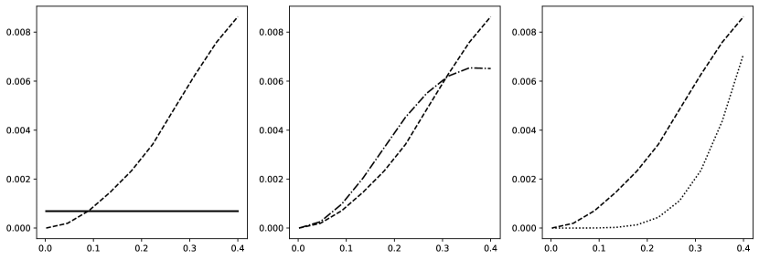
Figure 1: $\mathsf{P}(K_{n}=k,\bm{Y}^{*}\in\mathrm{d}\bm{y}^{*})$ when $n=5$, $\alpha=1$, as a function of the parameter $x$ under different settings. Left plot, setting (I) under the Poisson process ( ) and DPP ( ) prior. Middle plot: setting (I) ( ) and setting (II) ( ) under the DPP prior. Right plot setting (I) ( ) and setting (III) ( ) under the DPP prior.

5 Bayesian Hierarchical Mixture Models

Discrete random probability measures are commonly employed as mixing measures in Bayesian mixture models to address clustering and density estimation. In a mixture model, instead of modeling observations via (1), we use the de Finetti measure $Q$ in (1) as a prior for latent variables $Y_{1},\ldots,Y_{n}$.

To encompass location-scale mixtures, it is convenient to consider random measures on an extended space $\mathbb{X}\times\mathbb{W}$, instead of $\mathbb{X}$ itself. Hence, we deal with the random measure

$$\tilde{\mu}(\cdot)=\sum_{j\geq 1}S_{j}\delta_{(X_{j},W_{j})},$$ (19)

obtained by marking the points in the point process $\Psi$ with i.i.d. marks $(W_{j})_{j\geq 1}$ from an absolutely continuous probability distribution over $\mathbb{W}$, whose density we will denote by $f_{W}(\cdot)$.

To formalize the mixture model, consider $\mathbb{Z}$-valued observations $Z_{1},\ldots,Z_{n}$ and a probability kernel $f:\mathbb{Z}\times\mathbb{X}\times\mathbb{W}\rightarrow\mathbb{R}_{+}$, such that $z\mapsto f(z\,|\,y,v)$ is a probability density over $\mathbb{Z}$ for any $(y,v)\in\mathbb{\mathbb{X}}\times\mathbb{W}$. We assume both $\mathbb{Z}$ and $\mathbb{W}$ to be Polish spaces, endowed with the associated Borel $\sigma$-algebras. More precisely, the statistical model with which we are dealing is the following.

$$Z_{i}\,|\,Y_{i},V_{i} \stackrel{{\scriptstyle\mbox{\scriptsize ind}}}{{\sim}}f(\cdot\,|\,Y_{i},V_{i}),\qquad i=1,\ldots,n$$ (20)

$$Y_{i},V_{i}\,|\,\tilde{\mu} \stackrel{{\scriptstyle\mbox{\scriptsize iid}}}{{\sim}}\frac{\tilde{\mu}}{\tilde{\mu}(\mathbb{X}\times\mathbb{W})}$$

$$\tilde{\mu} \sim\mathbf{P}_{\mu}.$$

Usually, the kernel $f(\cdot\,|\,Y_{i},V_{i})$ is the Gaussian density with mean $Y_{i}$ and variance (if data are univariate) or covariance matrix (if data are multivariate) $V_{i}$, where the points $X_{j}$’s are the component-specific means and the points $W_{j}$’s the component-specific variances in a Gaussian mixture model. Note that, in accordance with previous literature on repulsive mixtures, we assume that the component-specific variances $V_{i}$’s are i.i.d. and that interaction is on the locations $Y_{i}$’s.

Let $M$ be the number of support points in $\tilde{\mu}$. It is convenient to introduce auxiliary component indicator variables $C_{i}$, $i=1,\ldots,n$ taking values in $1,\ldots,M$, such that $\mathsf{P}(C_{i}=h\,|\,\tilde{\mu})\propto S_{h}$. Noting that $(Y_{i},V_{i})_{i\geq 1}=(X_{C_{i}},W_{C_{i}})_{i\geq 1}$, (20) is equivalent to

$$Z_{i}\,|\,\tilde{\mu},C_{i} \stackrel{{\scriptstyle\mbox{\scriptsize ind}}}{{\sim}}f(\cdot\,|\,X_{C_{i}},W_{C_{i}}),\qquad i=1,\ldots,n$$ (21)

$$C_{i}\,|\,\tilde{\mu} \stackrel{{\scriptstyle\mbox{\scriptsize iid}}}{{\sim}}\mbox{Categorical}(S_{1}/T,\ldots,S_{m}/T)$$

$$\tilde{\mu} \sim\mathbf{P}_{\mu}$$

where $T:=\sum_{j\geq 1}S_{j}$. Following the standard terminology of (Argiento and De Iorio, 2022; Griffin and Walker, 2011), we define $\bm{S}^{(a)}=(S^{(a)}_{1},\ldots,S^{(a)}_{K_{n}})$ as the distinct values in $(S_{C_{i}})_{i\geq 1}$ and refer to them as active jumps. Moreover, we set the non-active jumps $\bm{S}^{(na)}:=\{S_{1},\ldots,S_{M}\}\setminus\bm{S}^{(a)}$. Analogously, we define $\bm{X}^{(a)},\bm{X}^{(na)}$ and $\bm{W}^{(a)},\bm{W}^{(na)}$ and refer to them as the active and non-active atoms, respectively. Note that, in this notation, $\bm{X}^{(a)}$ coincide with the unique values in the latent variables $Y_{1},\ldots,Y_{n}$ in (20). Thanks to exchangeability, we can always assume that $(X^{(a)}_{1},\ldots,X^{(a)}_{K_{n}})$ are the first $K_{n}$ points of $(X_{1},\ldots,X_{M})$.

In the rest of this section, we describe two Markov chain Monte Carlo algorithms for posterior inference under model (20). These are based on the posterior characterization of $\tilde{\mu}$ given $Y_{1},\ldots,Y_{n}$ in Theorem 4.1 and the predictive distribution of $Y_{n+1}$ in Theorem 4.3. Following Papaspiliopoulos and Roberts (2008), we term them conditional and marginal algorithms, respectively. In fact, in the former, the random measure $\tilde{\mu}$ is part of the state space of the algorithm, while in the latter, $\tilde{\mu}$ is integrated out. We assume that, conditionally to the number of points $M$, the distribution of the vector $(X_{1},\ldots,X_{M})\in\mathbb{X}^{M}$ defining the support of $\Phi$ has a density. With an abuse of notation, we denote this density by $f_{\Phi}$; the existence of the density of the point process $\Phi$ guarantees that the $f_{\Phi}$ above is indeed proportional to the density of the point process itself (see Møller and Waagepetersen (2003) for more details).

5.1 A conditional MCMC algorithm

A trivial extension of Theorem 4.1, to encompass for i.i.d. marks $(W_{j})_{j\geq 1}$, can be used to derive the full-conditional of $\tilde{\mu}$ given $C_{1},\ldots,C_{n},\bm{X}^{(a)},\bm{W}^{(a)}$ and $U_{n}$.

Corollary 5.1.

Consider the model (21), and define $n_{h}=\sum_{i=1}^{n}\mathbbm{1}_{h}(C_{i})$. Then, conditionally on $C_{1},\ldots,C_{n},K_{n}=k,\bm{X}^{(a)}=\bm{x}^{(a)},\bm{W^{(a)}}=\bm{w}^{(a)}$ and $U_{n}=u$, $\tilde{\mu}$ is equal to the distribution to

$$\sum_{h=1}^{k}S^{(a)}_{h}\delta_{(x^{(a)}_{h},w^{(a)}_{h})}+\tilde{\mu}^{\prime}$$

where $S^{(a)}_{h}\sim f_{S^{(a)}_{h}}(s)\propto s^{n_{h}}{\rm e}^{-us}H(\mathrm{d}s)$, and $\tilde{\mu}^{\prime}:=\sum_{h\geq 1}S^{(na)}_{h}\delta_{(X^{(na)}_{h},W^{(na)}_{h})}$ is obtained by considering the random measure at point (ii) in Theorem 4.1 and adding i.i.d. marks $W^{(na)}_{h}\sim f_{W}$ to the support points.

Corollary 5.1 leads to the algorithm below, where we write “$\cdot\,|\,\text{rest}$” to mean that we are conditioning with respect to all the variables but the ones appearing on the left hand side of the conditioning symbol.

1. Sample $U_{n}\,|\,\text{rest}\sim\mbox{Gamma}(n,T)$, where $T:=\sum_{j=1}^{m}S_{j}$.

2. Sample each $C_{i}$ independently from a discrete distribution over $\{1,\ldots,M\}$ such that

   $$\mathsf{P}(C_{i}=h\,|\,\text{rest})\propto S_{h}f(Z_{i}\,|\,X_{h},W_{h})$$

   Let $k$ be the number of the unique values in $\bm{X}^{(a)}:=\{X_{C_{i}},\ i=1,\ldots,n\}$. Define $\bm{W}^{(a)}$ and $\bm{S}^{(a)}$ analogously. Then, relabel $\bm{S}$, $\bm{X}$ and $\bm{W}$ so that $X_{1},\ldots,X_{k}$ equals $\bm{X}^{(a)}$ and analogously for $\bm{S}$, $\bm{W}$ with respect to $\bm{S}^{(a)}$, $\bm{W}^{(a)}$.

3. Sample $\tilde{\mu}$ using the distribution in Corollary 5.1. For the active part, sample each $S^{(a)}_{h}$ independently from a distribution on $\mathbb{R}_{+}$ with density

   $$f_{S_{h}}(s)\propto{\rm e}^{-Us}s^{n_{h}}H(\mathrm{d}s).$$

   For the non-active part, first sample $\sum_{j\geq 1}S^{(na)}_{j}\delta_{X^{(na)}_{j}}$ from the law of a random measure with Laplace transform (13). See below for some guidelines on how to perform this step. Then sample the corresponding marks $W^{(na)}_{j}\stackrel{{\scriptstyle\mbox{\scriptsize iid}}}{{\sim}}f_{W}$.

4. Sample $\bm{X}^{(a)}$ from the density on $\mathbb{X}^{k}$ given by

   $$\mathsf{P}(\bm{X}^{(a)}\in\mathrm{d}\bm{x}\,|\,\text{rest})\propto f_{\Phi}(\bm{x},\bm{X}^{(na)})\prod_{h=1}^{k}\prod_{i:C_{i}=h}f(Y_{i}\,|\,x_{h},W_{h}),\quad\bm{x}\in\mathbb{X}^{k}$$

5. Sample each entry in $\bm{W}^{(a)}$ independently from a density on $\mathbb{R}_{+}$ proportional to

   $$f_{W}(w)\prod_{i:C_{i}=h}f(Y_{i}\,|\,X^{(a)}_{h},w)$$

6. Set $\bm{X}=(\bm{X}^{(a)},X^{(na)})$, $\bm{W}=(\bm{W}^{(a)},\bm{W}^{(na)})$ $\bm{S}=(\bm{S}^{(a)},\bm{S}^{(na)})$ and $m$ equal to the length of these vectors.

Among the steps in the algorithm, the most complex is the third, which involves the sampling of the random measure $\tilde{\mu}^{\prime}$ with a given Laplace transform. In fact, all the remaining ones can be handled either by closed form full-conditionals (depending for instance on the law of the jumps $H(\mathrm{d}s)$ and the prior $f_{W}$) or by simple Metropolis-Hastings steps. To sample $\tilde{\mu}^{\prime}$, first sample its support points $\Phi^{\prime}=\sum_{j\geq 1}\delta_{X^{(na)}_{j}}$. This can be done either via perfect sampling (e.g., Algorithm 11.7 in Møller and Waagepetersen (2003)) or via a birth-death Metropolis-Hastings step (e.g., Algorithm 11.3 in Møller and Waagepetersen (2003)). Then sample the corresponding jumps $S^{(na)}_{j}\stackrel{{\scriptstyle\mbox{\scriptsize iid}}}{{\sim}}f_{S_{j}}\propto{\rm e}^{-Us}H(\mathrm{d}s)$ and the marks $W^{(na)}_{j}\stackrel{{\scriptstyle\mbox{\scriptsize iid}}}{{\sim}}f_{W}$. For instance, when $\Phi$ is a Gibbs point process with a density, the algorithm coincides with that in Beraha et al. (2022), where the update of $\tilde{\mu}^{\prime}$ was performed using a birth-and-death Metropolis-Hastings algorithm. On the other hand, when considering a DPP prior, we we can use Algorithm 1 in Lavancier et al. (2015) to obtain a perfect sample from the law of $\bm{X}^{(na)}$. We expect this choice to yield superior performance in terms of mixing.

5.2 A marginal MCMC algorithm

When integrating out $\tilde{\mu}$ from (20), Theorem 4.3 can be used to devise a marginal MCMC strategy. Using the generalized Chinese restaurant restaurant metaphor, at every iteration of the MCMC algorithm, each customer is removed from the restaurant and re-enters following the conditional distribution in Theorem 4.3. The plain application of this result yields the following MCMC algorithm.

1. Sample $U_{n}\,|\,\text{rest}$ from the full conditional distribution in (14).

2. For each observation, sample $(Y_{i},V_{i})$ from

   $$\mathsf{P}((Y_{i},V_{i})\in(\mathrm{d}y\,\mathrm{d}v)\,|\,\text{rest})\propto\sum_{j=1}^{k}\frac{\kappa(u,n^{(-i)}_{j}+1)}{\kappa(u,n^{(-i)}_{j})}f(Z_{i}\,|\,Y_{j}^{*},V^{*}_{j})\delta_{(Y_{j}^{*},V^{*}_{j})}(\mathrm{d}y\,\mathrm{d}v)+\\ \kappa(u,1)\frac{\mathsf{E}\left[{\rm e}^{-\int_{\mathbb{X}}u\tilde{\mu}_{\bm{y}^{*(-i)},y}^{!}(\mathrm{d}z)}\right]}{\mathsf{E}\left[{\rm e}^{-\int_{\mathbb{X}}u\tilde{\mu}_{\bm{y}^{*(-i)}}^{!}(\mathrm{d}z)}\right]}\int_{\mathbb{X}\times\mathbb{W}}\frac{m_{\Phi^{k+1}}(\bm{y}^{*(-i)},y)}{m_{\Phi^{k}}(\bm{y}^{*(-i)})}f(Z_{i}\,|\,y,v)P_{0}(\mathrm{d}y)f_{W}(v)\mathrm{d}v,$$

   where the superscript $(-i)$ means that the $i$-th observation is removed from the state for the computations. Here, $\bm{Y}^{*}$ and $\bm{V}^{*}$ are the vectors of unique values in $(Y_{1},\ldots,Y_{n})$ and $(V_{1},\ldots,V_{n})$ respectively.

3. Sample the unique values $\bm{Y}^{*}$ from a joint distribution on $\mathbb{X}^{k}$ proportional to

   $$\mathsf{P}(\bm{Y}^{*}\in\mathrm{d}\bm{y}^{*})\propto f_{\Phi}(\bm{x})\prod_{h=1}^{k}\prod_{\{i:\,Y_{i}=Y^{*}_{h}\}}f(Z_{i}\,|\,y^{*}_{h},V^{*}_{h}),\quad\bm{y}^{*}\in\mathbb{X}^{k}.$$

4. Sample each of unique values $\bm{V}^{*}$ independently from

   $$\mathsf{P}(V^{*}_{h}\in\mathrm{d}v^{*})\propto f_{W}(v)\prod_{i:C_{i}=h}f(Y_{i}\,|\,Y^{*}_{h},v^{*}),\quad v^{*}\in W.$$

Step 2 of the algorithm above requires the computation of

$$\int_{\mathbb{X}\times\mathbb{W}}\frac{m_{\Phi^{k+1}}(\bm{y}^{*(-i)},y)}{m_{\Phi^{k}}(\bm{y}^{*(-i)})}f(Z_{i}\,|\,y,v)P_{0}(\mathrm{d}y)f_{W}(v)\mathrm{d}v$$

which might be challenging is situations where data are multidimensional. However, Xie and Xu (2019) show how this can be overcome using numerical quadrature. Moreover, in higher dimensional setting we can adapt the strategy devised by Neal in his Algorithm 8, by introducing $L$ auxiliary variables and replace Step 2 with

1. for $\ell=1,\ldots,L$, sample $Y^{*}_{k+\ell}$ from

   $$\mathsf{P}(Y^{*}_{k+\ell}\in\mathrm{d}y\,|\,\text{rest})\propto\frac{m_{\Phi^{k+1}}(\bm{y}^{*(-i)},y)}{m_{\Phi^{k}}(\bm{y}^{*(-i)})}P_{0}(\mathrm{d}y)$$

   and $V^{*}_{k+\ell}\stackrel{{\scriptstyle\mbox{\scriptsize iid}}}{{\sim}}f_{W}$.

2. Set $(Y_{i},V_{i})$ equal to $(Y^{*}_{h},V^{*}_{h})$ with probability proportional to

   $$\frac{\kappa(u,n^{(-i)}_{j}+1)}{\kappa(u,n^{(-i)}_{j})}f(Z_{i}\,|\,Y_{h}^{*},V^{*}_{h}),\qquad h=1,\ldots,k$$

   $$\frac{1}{L}\kappa(u,1)\frac{\mathsf{E}\left[{\rm e}^{-\int_{\mathbb{X}}u\tilde{\mu}_{k+1}^{!}(\mathrm{d}z)}\right]}{\mathsf{E}\left[{\rm e}^{-\int_{\mathbb{X}}u\tilde{\mu}_{k}^{!}(\mathrm{d}z)}\right]}f(Z_{i}\,|\,Y_{h}^{*},V^{*}_{h}),\qquad h=k+1,\ldots,k+L.$$

   The computation of the ratio of expected values can be challenging, see Examples 4.8 and 4.9 for possible strategies.

6 Shot-Noise Cox Process and its use in mixture models

In this section we specialize all the previous results on a noteworthy example of Cox processes (Cox, 1955), namely, the shot-noise Cox process, introduced in Møller (2003). Then, in Section 6.1, we discuss its use in mixture models and how this gives rise to a nonparametric generalization of mixtures of mixtures in the sense of Malsiner-Walli et al. (2017). We finally provide a numerical illustration at the end of the present section.

In what follows, we assume that $\mathbb{X}\subset\mathbb{R}^{q}$. A shot-noise Cox process (SNCP) $\Phi$ is defined as

$$\Phi\,|\,\Lambda\sim\mbox{PP}(\omega_{\Lambda}),\quad\omega_{\Lambda}(\mathrm{d}x)=\gamma\left(\int_{\mathbb{X}}k_{\alpha}(x-v)\Lambda(\mathrm{d}v)\right)\mathrm{d}x,\quad\Lambda\sim\mbox{\rm PP}(\omega)$$ (22)

where $\mbox{PP}(\omega_{\Lambda})$ and $\mbox{PP}(\omega)$ denote Poisson processes with intensity $\omega_{\Lambda}$ and $\omega$, respectively. Here, $k_{\alpha}$ is a probability density with respect to the $q$-dimensional Lebesgue measure and $\gamma>0$. In particular, by assuming that $x\mapsto k_{\alpha}(x-v)$ is continuous for any $v$, we get that the point process $\Phi$ is simple. We refer to $\omega$ as the base intensity of the process $\Phi$.

It is easy to see that $M_{\Phi}(A)=\int_{A}m_{\Phi}(x)\mathrm{d}x=\gamma\int_{A}\int_{\mathbb{X}}k_{\alpha}(x-v)\omega(\mathrm{d}v)\mathrm{d}x$. See Lemma G.3 and Lemma G.1 in the Appendix for the calculation of the $n$-th moment measure and the Palm version of shot-noise Cox processes, respectively. In particular, by putting

$$\eta(x_{1},\ldots,x_{l})=\int\prod_{i=1}^{l}k_{\alpha}(x_{i}-v)\omega(\mathrm{d}v)$$ (23)

and using Lemma G.3, we specialize expressions in Proposition 3.1 as follows

$$\mathsf{E}[\tilde{\mu}(A)] =\mathsf{E}[S]\gamma\int_{A}\eta(x)\mathrm{d}x$$

$$\mbox{Cov}(\tilde{\mu}(A),\tilde{\mu}(B)) =\mathsf{E}[S^{2}]\gamma^{2}\int_{A\times B}\eta(x_{1},x_{2})\mathrm{d}x_{1}\mathrm{d}x_{2}.$$

However, the moments of the associated normalized measure $\tilde{p}$ involve intractable integrals and are not reported here.
The following result specializes Theorem 4.1 in the case of shot-noise Cox processes.

Theorem 6.1.

Assume that $\Phi$ is a shot-noise Cox process with base intensity $\omega(\mathrm{d}x)$. Then, the random measure $\tilde{\mu}^{\prime}$ in (12) can be decomposed as

$$\tilde{\mu}^{\prime}\stackrel{{\scriptstyle d}}{{=}}\tilde{\mu}_{0}+\sum_{h=1}^{k}\tilde{\mu}_{\zeta_{h}},$$

where $\tilde{\mu}_{0}=\sum_{j\geq 1}\tilde{S}_{j}\delta_{\tilde{X}_{j}}$ and $\tilde{\mu}_{\zeta_{h}}=\sum_{j\geq 1}\tilde{S}_{h,j}\delta_{\tilde{X}_{h,j}}$ are independent. The unmarked point processes $\Phi_{0}=\sum_{j\geq 1}\delta_{\tilde{X}_{j}}$ is a shot-noise Cox process with base intensity

$$\omega^{\prime}(\mathrm{d}x)={\rm e}^{-\gamma(1-\psi(u))}\omega(\mathrm{d}x),$$

each $\Phi_{\zeta_{h}}=\sum_{j\geq 1}\delta_{\tilde{X}_{h,j}}$ is a Poisson point process with random intensity

$$\omega_{\zeta_{h}}(\mathrm{d}x)={\rm e}^{-\gamma(1-\psi(u))}k_{\alpha}(\zeta_{h}-x)\mathrm{d}x,$$

and the $\zeta_{h}$’s are independent random variables on $(\mathbb{X},\mathcal{X})$ with density

$$\zeta_{h}\sim p_{\zeta_{h}}(y)\propto\gamma k_{\alpha}(x_{j}-y_{j})\lambda(\mathrm{d}y_{j}).$$

Moreover, all the weights of $\tilde{\mu}_{0}$ and the $\tilde{\mu}_{\zeta_{h}}$’s are i.i.d. with distribution

$$H^{\prime}(\mathrm{d}s):=\frac{{\rm e}^{-su}H(\mathrm{d}s)}{\int_{\mathbb{R}^{+}}{\rm e}^{-su}H(\mathrm{d}s)}.$$

Without loss of generality, hereafter we assume that the base measure $\omega(\mathrm{d}x)$ integrates to 1. Theorem 4.2 simplifies to the following statement. See Section G.3 for the details.

Proposition 6.2.

Consider the model (1) and assume that $\mathbf{P}_{\Phi}$ is the law of a shot-noise Cox process, then the marginal distribution of a sample $\bm{Y}$ equals

$$\mathsf{P}(\bm{Y}\in\mathrm{d}\bm{y}) =\int_{\mathbb{R}_{+}}\frac{u^{n-1}}{\Gamma(n)}\exp\left\{\lambda\left({\rm e}^{\gamma(\psi(u)^{-1}-1)}-1\right)+k\gamma(\psi(u)^{-1}-1)\right\}\prod_{j=1}^{k}\kappa(u,n_{j})\mathrm{d}u$$

$$\times\gamma^{k}\sum_{j=1}^{k}\sum_{C_{1},\ldots C_{j}\in(*)}\prod_{l=1}^{j}\eta(\bm{y}^{*}_{C_{l}})\mathrm{d}y^{*}_{1}\cdots\mathrm{d}y^{*}_{k},$$

where $k$ is the number of distinct values in $\bm{y}$, $(*)$ denotes all the partitions of $k$ elements in $j$ groups and $\eta(\cdot)$ is as in (23).

From Corollary 4.5 and Proposition 6.2 it is now straightforward to derive the marginal distribution of the distinct values. Indeed, from Lemma G.1 in the Appendix, we have that the total mass in the reduced Palm version of $\Phi$ satisfies $\Phi^{!}_{\bm{y}}(\mathbb{X})\,|\,\Lambda\sim\mbox{Poi}(\gamma(k+\Lambda(\mathbb{X}))$ and $\Lambda(\mathbb{X})\sim\mbox{Poi}(\lambda)$. Hence, $q_{r}=:\mathsf{P}(\Phi^{!}_{\bm{y}}(\mathbb{X})=r)$ does not depend on the values in $\bm{y}^{*}$, but only on its cardinality. Observe that the moment measure of $\Phi$ is

$$M_{\Phi}^{k}(\mathrm{d}\bm{x})=\gamma^{k}\sum_{j=1}^{k}\sum_{C_{1},\ldots C_{j}\in(*)}\prod_{l=1}^{j}\eta(\bm{x}_{C_{l}})\mathrm{d}x_{1}\cdots\mathrm{d}x_{k}.$$

See Lemma G.3 in the Appendix for a proof. Hence, starting for the expression provided in Corollary 4.5 and marginalizing with respect to $\bm{y}^{*}$, we have

$$\mathsf{P}(K_{n}=k)=\frac{1}{\Gamma(n)}\gamma^{k}(-1)^{k}\mathcal{C}(n,k;-\alpha)B_{k}\sum_{r\geq 0}q_{r}\frac{\Gamma(k+r)\alpha}{\Gamma((k+r)\alpha+n)},$$

where $B_{k}$ is the $k$-th Bell number and $\mathcal{C}(n,k;-\gamma)$ is the generalized factorial coefficient. This expression holds in the case of $\mbox{Gamma}(\alpha,1)$ distributed jumps.

To conclude, the predictive distribution from Theorem 4.3 under the shot-noise Cox process model equals

$$\mathsf{P}(Y_{n+1}\in A\,|\,\bm{Y}=\bm{y},U_{n})\propto\sum_{j=1}^{k}\frac{\kappa(U_{n},n_{j}+1)}{\kappa(U_{n},n_{j})}\delta_{Y_{j}^{*}}(A)\\ +\int_{A}\kappa(U_{n},1)\exp\left\{\gamma(\psi(u)^{-1}-1)\right\}\frac{m_{\Phi^{k+1}}(\bm{y}^{*},y)}{m_{\Phi^{k}}(\bm{y}^{*})}P_{0}(\mathrm{d}y).$$

6.1 SNCP mixtures as mixtures of mixtures

We now focus on the use of a SNCP as a mixing measure in mixture models. First, we note that, by the coloring theorem for Poisson point processes (Kingman, 1992), the conditional distribution of $\Phi$ given $\Lambda$ equals the distribution of $\sum_{\lambda_{j}\in\Lambda}\Phi_{j}$, where $\Phi_{j}\,|\,\Lambda$ is a Poisson point process with intensity $\gamma k_{\alpha}(x-\lambda_{j})$. This shows that SNCPs are cluster processes (see, e.g., Daley and Vere-Jones, 2003). In this context instead of referring to the $\Phi_{j}$’s as clusters, we denote them as groups to avoid misunderstandings with the usual BNP notation. Observe that, for appropriate choices of $k_{\alpha}$, the points in a group will be closer than points belonging to different groups. When we embed a random probability measure built from (22) in a Bayesian mixture model as done in Section 5, we obtain that the atoms of the mixture are randomly grouped together. Hence, we rewrite the random population density as

$$f(z)=\frac{1}{T}\sum_{h\geq 1}\tilde{S}_{h}f(z\,|\,X_{h},W_{h})\equiv\frac{1}{T}\sum_{j=1}^{n(\Lambda)}\sum_{h\geq 1}\tilde{S}_{j,h}f(z\,|\,\tilde{X}_{j,h},\tilde{W}_{j,h})$$

where, on the right hand side, we first sum over the atoms of $\Lambda$ and then over the atoms of each of the groups $\Phi_{j}$’s. With an abuse of notation, we have introduced a second subscript to $\tilde{S}_{h}$, $\tilde{X}_{h}$, and $\tilde{W}_{h}$ to keep track that each point of $\tilde{X}_{h}$ (and its marks) is assigned to a point in $\Lambda$. Let us define

$$\tilde{f}_{j}(z):=\frac{1}{P_{j}}\sum_{h\geq 1}\tilde{S}_{j,h}f(z\,|\,\tilde{X}_{j,h},\tilde{W}_{j,h}),\ \textrm{where }P_{j}:=\sum_{h\geq 1}\tilde{S}_{j,h},$$ (24)

which is a (random) probability density function over $\mathbb{X}$. We clearly see that the random population density is equal to $f(z)=T^{-1}\sum_{j=1}^{n(\Lambda)}P_{j}\tilde{f}_{j}(z)$. Hence, a SNCP mixture model can be written as a mixture of mixtures, where each component $\tilde{f}_{j}(z)$ is expressed as a mixture model itself. Therefore, we can consider the SNCP mixture model as a nonparametric generalization of the mixture of mixtures model in Malsiner-Walli et al. (2017). In the frequentist setting, identifiability and estimation of the mixture of mixtures model have recently been studied in Aragam et al. (2020).

Observe that the SNCP mixture induces a two-level clustering. At the first level, the parameters $(Y_{i},V_{i})$ in (20) induce the standard partition of the observations by the equivalence relation $i\sim j$ if and only if $(Y_{i},V_{i})=(Y_{j},V_{j})=(X_{h},W_{h})$ for some $h$. Let $c_{i}=h$ if and only if $(Y_{i},V_{i})=(X_{h},W_{h})$. Then, at the second level, each point $(X_{h},W_{h})$ can be referred to one of the groups $\Phi_{j}$. We introduce a variable $t_{h}$ for each of the $(X_{h},W_{h})$ such that $t_{h}=j$ if and only if $X_{h}\in\Phi_{j}$. Hence, we can refer observations to the groups using the variables $(t_{c_{1}},\ldots,t_{c_{n}})$. In the next subsection, we call the partition induced by the $t_{c_{i}}$’s as the grouping of the observations.

6.2 Numerical illustration

We consider a simulated scenario where 200 datapoints are generated from a two-component mixture of univariate Student’s $t$ distributions with degrees of freedom equal to three, centered respectively in $-5$ and $+5$. We fit a mixture of Gaussian distributions to the dataset, i.e., $f$ in (20) is the Gaussian density where parameters $(Y_{i},V_{i})$ are the mean and the variance, respectively. For the distribution $f_{W}$ of the $W_{j}$’s, we assume an inverse-Gamma density with both shape and scale parameters equal to two. The prior for $\Phi$ is the shot-noise Cox process with $\alpha=1$ and $\gamma=1$. The unnormalized weights are $S_{j}\stackrel{{\scriptstyle\mbox{\scriptsize iid}}}{{\sim}}\mbox{Gamma}(2,2)$.

We compare the SNCP mixture to the normalized IFPP mixture model in Argiento and De Iorio (2022), where their mixing measure $\mu$ is as in (19) and the number of support points $K$ is such that $K-1\sim\mbox{Poi(2)}$. Given $K$, the support points $(X_{j},W_{j})$ are assumed i.i.d. from a Normal-inverse-gamma density, i.e., $X_{j}|W_{j}\sim\mathcal{N}(0,10W_{j})$ and $1/W_{i}\sim\mbox{Gamma}(2,2)$. The unnormalized weights $S_{j}$ are given the same prior as for the SNCP mixture model. Posterior inference for the model in Argiento and De Iorio (2022) is computed via the BayesMix library (Beraha et al., 2022).

To fit the SNCP mixture, we use the conditional algorithm in Section 5.1, where we further add to the MCMC state the points of $\Lambda$; see Section G.4 for further details. The Python code is available at https://github.com/mberaha/sncp_mix.

The SNCP mixture activates between 25 and 40 Gaussian components to represent the mixture of Student $t$’s distribution, while the normalized IFPP mixture uses only between 3 and 8 active components. We compare the grouping of the datapoints induced by the SNCP mixture, as defined above, with the standard clustering induced by the normalized IFPP mixture. Posterior inference is summarized in Figure 2. In particular, the figure displays the posterior co-clustering matrix under the two models (panels (a) and (b)), i.e., for any couple of observations $i$ and $j$, the probability that $i$ and $j$ are assigned to the same cluster/group, the posterior of the number of clusters/groups (panel (c)) and the density estimate (panel (d)) under the two models. It is clear that the SNCP mixture does a better job in dividing data into two groups, while, the posterior probability of having two clusters under normalized IFPP is zero. Moreover, the posterior co-clustering matrix in the figure shows that the non-attractive mixture activates extra clusters, associating together observations near zero and on the extreme tails. In misspecified settings, there is a trade-off between the accuracy of the density and number of clusters estimation recovered by standard BNP mixtures. In fact, to recover the shape of non-Gaussian data, several Gaussian components in the mixtures are needed. See Beraha et al. (2022). Instead, in our model, a group is made up of several activated components, leading to a parsimonious data partition.

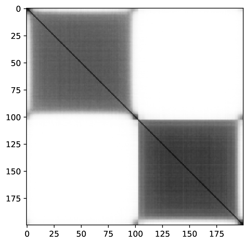
(a)

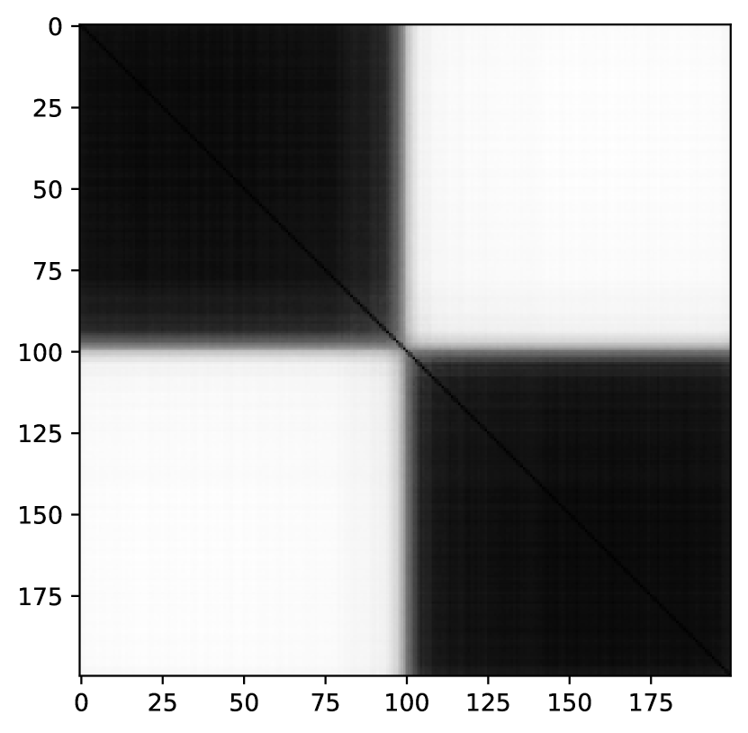
(b)

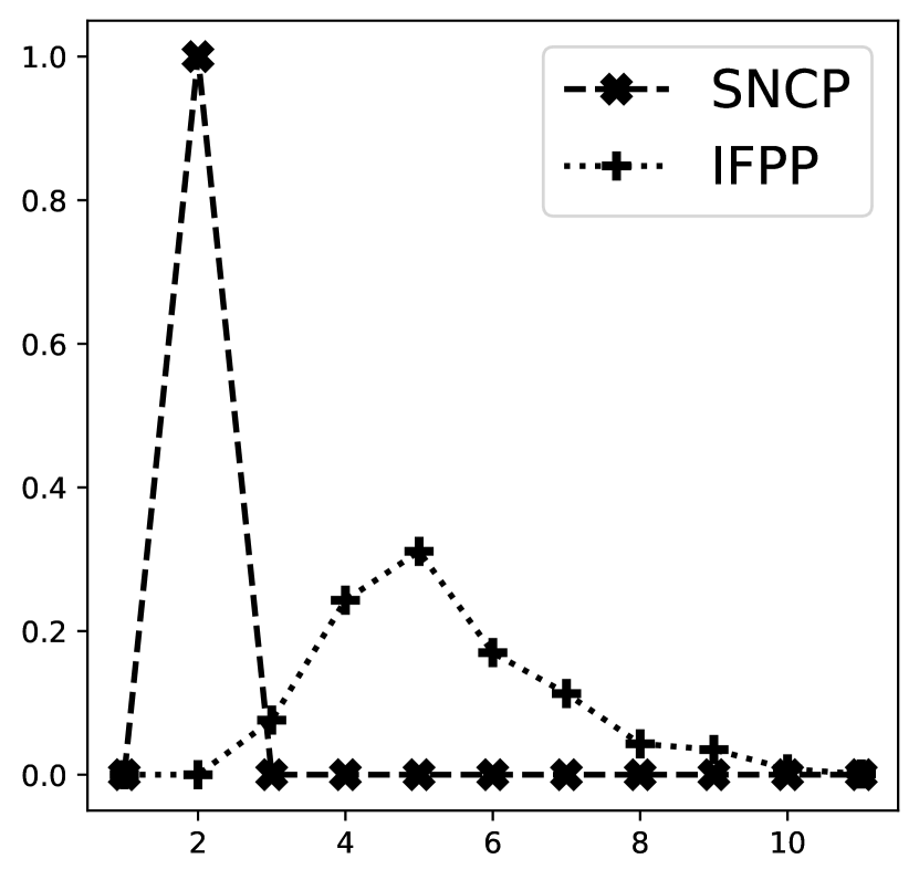
(c)

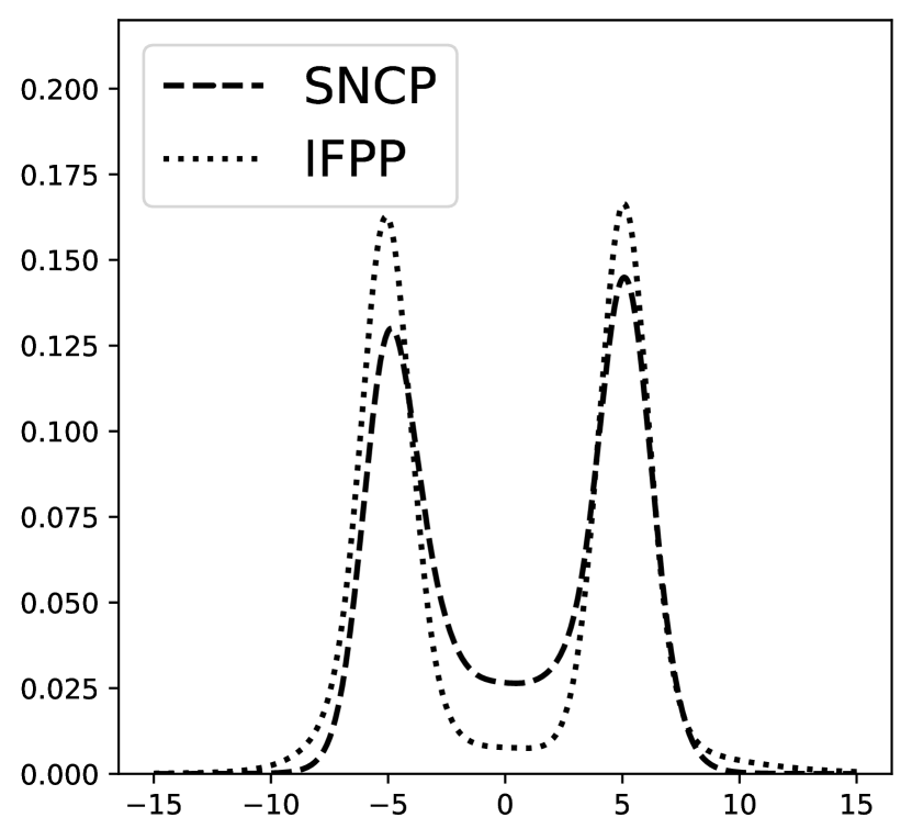
(d)

Figure 2: From left to right: posterior co-clustering matrix under the normalized IFPP (a) and SNCP (b) mixtures, posterior distribution of the number of clusters (c), density estimates (d). In the posterior co-clustering matrices, data are sorted from the smallest to the largest.

7 Discussion

In this work, we have investigated discrete random probability measures with interaction across support points. Our study is motivated by the recent popularity of repulsive mixtures Petralia et al. (2012); Quinlan et al. (2020); Xu et al. (2016); Bianchini et al. (2020); Beraha et al. (2022) for Bayesian model-based clustering. In contrast, the typical postulate in Bayesian mixture models is that the atoms of the a.s. discrete random mixing measure are i.i.d. from a base distribution. This assumption is usually associated with poor performance in cluster detection as shown in Cai et al. (2021); see also Guha et al. (2021) for related asymptotic properties. Assuming (repulsive) interaction across the support points practically mitigates this issue. The distributional properties of such kind of models are largely unexplored in the current literature, which results in both the lack of understanding of the effect of prior hyperparameters, which are often fixed using heuristics, and the development of ad hoc posterior simulation algorithms that might be inefficient.

Our first main contribution in this paper is to propose a general construction of RPMs via normalization of marked point processes. We use a simple and fundamental idea behind the construction of almost surely discrete random measures; i.e., they can be obtained by normalization of stochastic point processes. A popular approach of this type is given by Regazzini et al. (2003), where the authors define NRMIs through Poisson processes. More recently, using the same idea, Argiento and De Iorio (2022) build the class of normalized IFPPs from independent finite point processes. Both approaches build a discrete RPM by normalizing a marked point process where the point process defines the jumps of the RPM and i.i.d. marks define the atoms. In our case, we revert the roles of the points and the marks and let the points define the atoms, while the marks are the (unnormalized) jumps of our RPM. This allows the construction of RPMs with repulsive or attractive support points, which can be embedded in a hierarchical mixture model as shown in Section 5.

The second contribution of this paper is to present a unified mathematical theory encompassing repulsive or attractive mixtures, as well as the IFPP mixtures in Argiento and De Iorio (2022). Our results can be seen as the counterparts of well-known distributional properties of NRMIs. Due to the generality of our framework, our proofs rely on new arguments based on Palm calculus; see Baccelli et al. (2020). In particular, for a sample from our new RPM, we are able to derive expressions for the posterior distribution of the unnormalized random measure, the marginal distribution of the sample, the prior distribution of the distinct values in the sample, and the predictive distribution of a new observation. These expressions are pivotal for inferential purposes, since they either help to fix prior hyperparameters or enter in the definition of MCMC algorithms for posterior calculation. Our general theory is illustrated through the examples of Poisson, Gibbs, and determinantal point processes, for which interpretable expressions are found that clarify the fundamental differences between NRMIs and measures with interacting support points.

As a final contribution, we discuss the use of shot-noise Cox processes, which were not previously considered in connection with Bayesian mixture models beyond Wang et al. (2022). In particular, we find that shot-noise Cox process mixtures are the nonparametric generalization of the mixture of mixtures model in Malsiner-Walli et al. (2017). While this latter paper consider finite mixtures, under our shot-noise Cox process mixtures, the density of each mixture component is modelled by a nonparametric mixture density. This model induces a two-level grouping of the observations that is particularly useful for clustering under misspecified likelihoods.

Future research topics include the investigation of the asymptotic properties of the proposed mixture models, such as the consistency of the mixing measure and posterior number of clusters, possibly under model misspecification, therefore extending the existing theory for RPMs with i.i.d. atoms Nguyen (2013, 2016); Guha et al. (2021). Moreover, several extensions of our framework are also possible, including the analysis of other types of processes. First, following the approach in Camerlenghi et al. (2019), we could build a vector of dependent random probability measures and use it as a nonparametric prior for partially exchangeable data. We could also consider other classes of models, such as latent feature (Broderick et al., 2013) or trait allocations models (James, 2017).

The algorithms proposed in Section 5 are general MCMC schemes applicable to any choice of point process prior. However, they might lack efficiency, especially for moderate or high-dimensional data. For specific classes of point processes, more adequate algorithms could be devised; see, for instance, Sun et al. (2022) for an alternative MCMC scheme tailored to the class of Matérn point processes. Future works will investigate more efficient MCMC algorithms, for instance similar to the split-merge algorithm in Jain and Neal (2004) or based on variational inference (Blei and Jordan, 2006) to handle moderately-dimensional observations and parametric spaces.

Appendix A Background on Palm calculus

The basic tool used in our computations is a disintegration of the Campbell measure of a point process $\Phi$ with respect to its mean measure $M_{\Phi}$, usually called Palm kernel or family of Palm distributions of $\Phi$. Below, we recall the main results needed later in this paper. For further details about Palm distributions and Palm calculus see, e.g., the papers Kallenberg (1984); Coeurjolly et al. (2017) or the monographs Kallenberg (2017) (Chapter 6), Daley and Vere-Jones (2008) (Chapter 13). Here, we adapt the notation from the recent monograph Baccelli et al. (2020) (Chapter 3).

Let $\mathbb{M}(\mathbb{X})$ the space of bounded measures on $\mathbb{X}$ and denote by $\mathcal{M}(\mathbb{X})$ its Borel $\sigma$-algebra. For a point process $\Phi$ on $\mathbb{X}$, let us denote the mean measure by $M_{\Phi}$, i.e., $M_{\Phi}(B):=\mathsf{E}[\Phi(B)]$ for all $B\in\mathcal{X}$. We define the Campbell measure $\mathcal{C}_{\phi}$ on $\mathbb{X}\times\mathbb{M}(\mathbb{X})$ as

$$\mathcal{C}_{\Phi}(B\times L)=\mathsf{E}\left[\Phi(B)\mathbbm{1}_{L}(\Phi)\right],\quad B\in\mathcal{X},L\in\mathcal{M}(\mathbb{X}).$$

Then, as a consequence of the Radon-Nikodym theorem, for any fixed $L$, there exists a $M_{\Phi}$-a.e. unique disintegration probability kernel $\{\mathbf{P}_{\Phi}^{x}(\cdot)\}_{x\in\mathbb{X}}$ of $\mathcal{C}_{\phi}$ with respect to $M_{\Phi}$, i.e.

$$\mathcal{C}_{\Phi}(B\times L)=\int_{B}\mathbf{P}_{\Phi}^{x}(L)M_{\Phi}(\mathrm{d}x)\quad B\in\mathcal{X},L\in\mathcal{M}(\mathbb{X}).$$

Note that, for any $x\in\mathbb{X}$, $\mathbf{P}_{\Phi}^{x}$ is the distribution of a random measure (specifically, a point process) on $\mathbb{X}$. See (Kallenberg, 2021, Theorem 31.1). Therefore, $\mathbf{P}_{\Phi}^{x}$ can be identified with the distribution of a point process $\Phi_{x}$ such that $\mathbf{P}_{\Phi}^{x}(L)=\mathsf{P}(\Phi_{x}\in L)$. In particular, Proposition 3.1.12 in Baccelli et al. (2020) shows that the point process $\Phi_{x}$ has almost surely an atom at $x$. This property allows for the interpretation of $\mathbf{P}_{\Phi}^{x}$ as the probability distribution of the point process $\Phi$ given that (conditionally to) it has an atom at $x$. $\Phi_{x}$ is called the Palm version of $\Phi$ at $x$.

Theorem A.1 (Campbell-Little-Mecke formula. Theorem 3.1.9 in Baccelli et al. (2020)).

Let $\Phi$ be a point process on $\mathbb{X}$ such that $M_{\Phi}$ is $\sigma$-finite. Denote with $\mathbf{P}_{\Phi}(\cdot)$ its law. Let $\{\mathbf{P}_{\Phi}^{x}(\cdot)\}_{x\in\mathbb{X}}$ a family of Palm distributions of $\Phi$. Then, for all measurable $g:\mathbb{X}\times\mathbb{M}(\mathbb{X})\rightarrow\mathbb{R}_{+}$, one has

$$\begin{split}&\mathsf{E}\left[\int_{\mathbb{X}}g(x,\Phi)\Phi(\mathrm{d}x)\right]\\ &\qquad=\int_{\mathbb{M}(\mathbb{X})\times\mathbb{X}}g(x,\nu)\nu(\mathrm{d}x)\mathbf{P}_{\Phi}(\mathrm{d}\nu)=\int_{\mathbb{X}\times\mathbb{M}(\mathbb{X})}g(x,\nu)\mathbf{P}_{\Phi}^{x}(\mathrm{d}\nu)\mathbb{M}_{\Phi}(\mathrm{d}x)\end{split}$$ (25)

In many applications to spatial statistics, formula (25), referred to as CLM formula, is stated in terms of the reduced Palm kernel $\mathbf{P}_{\Phi^{!}}^{x}$, i.e.,

$$\mathsf{E}\left[\int_{\mathbb{X}}g(x,\Phi-\delta_{x})\Phi(\mathrm{d}x)\right]=\int_{\mathbb{X}\times\mathbb{M}(\mathbb{X})}g(x,\nu)\mathbf{P}_{\Phi^{!}}^{x}(\mathrm{d}\nu)\mathbb{M}_{\Phi}(\mathrm{d}x)$$

where $\Phi-\delta_{x}$ is obtained by removing the point $x$ from $\Phi$ and $\mathbf{P}_{\Phi^{!}}^{x}$ is the distribution of the point process

$$\Phi^{!}_{x}:=\Phi_{x}-\delta_{x}.$$

Hence, given a reduced Palm kernel, we can construct the non-reduced one by considering the distribution of $\Phi^{!}_{x}+\delta_{x}$.

Given a point process $\Phi$ define the $k$-th Campbell measure

$$\mathcal{C}^{k}_{\Phi}(B\times L)=\mathsf{E}\left[\int_{B}\mathbbm{1}_{L}(\Phi)\Phi^{k}(\mathrm{d}\bm{x})\right],\quad B\in\mathcal{X}^{\otimes k},L\in\mathcal{M}(\mathbb{X})$$

where $\mathrm{d}\bm{x}=\mathrm{d}x_{1}\cdots\mathrm{d}x_{k}$ and $\Phi^{k}(\mathrm{d}\bm{x})=\prod_{i=1}^{k}\Phi(\mathrm{d}x_{i})$. Let $M_{\Phi}^{k}$ be the mean measure of $\Phi^{k}$, i.e., $M_{\Phi^{k}}(B)=\mathcal{C}^{k}(B\times\mathcal{M}(\mathbb{X}))$, then the $k$–th Palm distribution $\{\mathbf{P}_{\Phi}^{\bm{x}}\}_{\bm{x}\in\mathbb{X}^{k}}$ is defined as the disintegration kernel of $C^{k}$ with respect to $M_{\Phi^{k}}$, that is

$$\mathcal{C}^{k}_{\Phi}(B\times L)=\int_{B}\mathbf{P}_{\Phi}^{\bm{x}}(L)M_{\Phi^{k}}(\mathrm{d}\bm{x}),\quad B\in\mathcal{X}^{\otimes k},L\in\mathcal{M}(\mathbb{X})$$

The following is a multivariate extension of Theorem A.1 that will be useful for later computations.

Theorem A.2 (Higher order CLM formula.).

Let $\Phi$ a point process on $\mathbb{X}$ such that $M_{\Phi^{k}}$ is $\sigma$-finite. Let $\{\mathbf{P}_{\Phi}^{\bm{x}}(\cdot)\}_{\bm{x}\in\mathbb{X}^{k}}$ a family of $k$–th Palm distributions of $\Phi$. Then, for all measurable $g:\mathbb{X}^{k}\times\mathbb{M}(\mathbb{X})\rightarrow\mathbb{R}_{+}$

$$\mathsf{E}\left[\int_{\mathbb{X}^{k}}g(\bm{x},\Phi)\Phi^{k}(\mathrm{d}\bm{x})\right]=\int_{\mathbb{X}^{k}\times\mathbb{M}(\mathbb{X})}g(\bm{x},\nu)\mathbf{P}_{\Phi}^{\bm{x}}(\mathrm{d}\nu)M_{\Phi^{k}}(\mathrm{d}\bm{x})$$ (26)

When $x_{1},\ldots,x_{k}$ are distinct, we have that the $k$-th moment measure $M_{\Phi^{k}}(\mathrm{d}\bm{x})$ coincides with the $k$-th factorial moment measure $M_{\Phi^{(k)}}$ defined as

$$M_{\Phi^{(k)}}(A_{1}\times\cdots\times A_{k})=\mathsf{E}\left[\sum_{(X_{1},\ldots,X_{k})\in\Phi}^{\neq}\mathbbm{1}_{A_{1}}(X_{1})\cdots\mathbbm{1}_{A_{k}}(X_{k})\right]$$

where the summation on the right hand side is over all the $k$-tuples in $\Phi$ of pairwise different elements. It is often convenient to work in terms of the factorial moment measure. In all of our computations, we can interchange the moment and factorial moment measures.

Appendix B Preparatory Lemmas

We now state some results relating to independently marked point processes

Lemma B.1.

Let $\Psi$ be an independently marked point process on $\mathbb{X}\times\mathbb{S}$ obtained by marking a point process $\Phi$ on $\mathbb{X}$ with i.i.d marks $(S_{j})_{j\geq 1}$ from a probability measure $H$, that does not depend on the value of the associated atom $X_{j}$. Then, the mean measure $M_{\Psi}$ is

$$M_{\Psi}(\mathrm{d}x\,\mathrm{d}s)=H(\mathrm{d}s)M_{\Phi}(\mathrm{d}x)$$

Analogously, if $M_{\Psi^{(n)}}$ is the $n$-th factorial mean measure of $\Psi$ , then it equals

$$M_{\Psi^{(n)}}(\mathrm{d}\bm{x}\,\mathrm{d}\bm{s})=H^{n}(\mathrm{d}\bm{s})M_{\Phi^{(n)}}(\mathrm{d}\bm{x})$$

which further equals $H^{n}(\mathrm{d}\bm{s})M_{\Phi^{n}}(\mathrm{d}\bm{x})$ since the sets are pairwise disjoint.

Proof.

Let $C=A\times B$, where $A\in\mathcal{X}$ $B\in\mathcal{S}$. We have that:

$$\mathsf{E}[\Psi(C)] =\mathsf{E}\left[\sum_{j\geq 1}\mathbbm{1}_{A\times B}(X_{j},S_{j})\right]=\mathsf{E}\left[\sum_{j\geq 1}\mathbbm{1}_{A}(X_{j})\mathbbm{1}_{B}(S_{j})\right]$$

$$=\sum_{j\geq 1}\mathsf{E}\left[\mathbbm{1}_{A}(X_{j})\mathbbm{1}_{B}(S_{j})\right]=\sum_{j\geq 1}H(B)\mathsf{E}\left[\mathbbm{1}_{A}(X_{j})\right]$$

$$=H(B)\mathsf{E}\left[\sum_{j\geq 1}\mathbbm{1}_{A}(X_{j})\right]=H(B)M_{\Phi}(B).$$

The proof for the $n$-th mean measure is achieved following the same steps with $A\in\mathcal{X}^{\otimes n}$ and $B\in\mathcal{S}^{\otimes n}$. ∎

Lemma B.2.

Let $\Psi$ be as in Proposition B.1, then the Palm distribution $\{\mathbf{P}_{\Psi}^{x,s}\}_{(x,s)\in\mathbb{X}\times\mathbb{S}}$ is the distribution of the point process $\delta_{(x,s)}+\Psi^{!}_{x,s}$, where $\Psi^{!}_{x,s}$ is an independently marked point process obtained by marking $\Phi^{!}_{x}\sim\mathbf{P}_{\Phi^{!}}^{x}$ with i.i.d marks from $H$. Similarly, let $(\bm{x},\bm{s})=(x_{1},\ldots,x_{n},s_{1},\ldots,s_{n})$, the Palm distribution $\{\mathbf{P}_{\Psi}^{\bm{x},\bm{s}}\}_{(\bm{x},\bm{s})\in\mathbb{X}^{n}\times\mathbb{S}^{n}}$ is the distribution of the point process $\sum_{i=1}^{n}\delta_{(x_{i},s_{i})}+\Psi^{!}_{\bm{x},\bm{s}}$, where $\Psi^{!}_{\bm{x},\bm{s}}$ is an independently marked point process obtained by marking $\Phi^{!}_{\bm{x}}\sim\mathbf{P}_{\Phi}^{\bm{x}}$ with i.i.d. marks from $H$.

Proof.

By the CLM formula for the reduced Palm kernel, we know that $\Psi^{!}_{x,s}$ satisfies

$$\mathsf{E}\left[\int_{\mathbb{X}\times\mathbb{S}}g(x,s,\Psi-\delta_{(x,s)})\Psi(\mathrm{d}x\,\mathrm{d}s)\right]=\int_{\mathbb{X}\times\mathbb{S}}\mathsf{E}\left[g(x,s,\Psi^{!}_{x,s})\right]M_{\Psi}(\mathrm{d}x\,\mathrm{d}s).$$ (27)

Consider now the point process $\Psi^{\prime}_{x,s}$ obtained by marking $\Phi^{!}_{x}$ with i.i.d marks from $H$, if

$$\int_{\mathbb{X}\times\mathbb{S}}\mathsf{E}\left[g(x,s,\Psi^{\prime}_{x,s})\right]M_{\Psi}(\mathrm{d}x\,\mathrm{d}s)=\int_{\mathbb{X}\times\mathbb{S}}\mathsf{E}\left[g(x,s,\Psi^{!}_{x,s})\right]M_{\Psi}(\mathrm{d}x\,\mathrm{d}s),$$ (28)

for any $g$, we can conclude that $\Psi^{\prime}_{x,s}$ and $\Psi^{!}_{x,s}$ are equal in distribution. To prove (28), we will show that

$$\int_{\mathbb{X}\times\mathbb{S}}\mathsf{E}\left[g(x,s,\Psi^{\prime}_{x,s})\right]M_{\Psi}(\mathrm{d}x\,\mathrm{d}s)=\mathsf{E}\left[\int_{\mathbb{X}\times\mathbb{S}}g(x,s,\Psi-\delta_{x,s})\Psi(\mathrm{d}x\,\mathrm{d}s)\right].$$

In the following, we write $E_{V}[f(x,z)]$ to indicate that the expectation is taken with respect to the generic random variable $V$. Write $\Psi^{\prime}=(\Phi^{!},\bm{m})$ where $\bm{m}$ is the collection of marks. With a slight abuse of notation, we write $g(x,s,\Psi^{\prime}_{x,s})=g(x,s,\Phi^{!}_{x},\bm{m})$. Then

$$\int_{\mathbb{X}\times\mathbb{S}} \mathsf{E}_{\Psi}\left[g(x,s,\Psi^{\prime}_{x,s})\right]M_{\Psi}(\mathrm{d}x\,\mathrm{d}s)=\int_{\mathbb{X}\times\mathbb{S}}\mathsf{E}_{\Phi^{!}_{x},\bf m}\left[g(x,s,\Phi^{!}_{x},\bm{m})\right]M_{\Psi}(\mathrm{d}x\,\mathrm{d}s)$$

$$=\int_{\mathbb{X}\times\mathbb{S}}\mathsf{E}_{\Phi^{!}_{x}}\left[\mathsf{E}_{\bf m}\left[g(x,s,\Phi^{!}_{x},\bm{m})\,|\,\Phi^{!}_{x}\right]\right]M_{\Psi}(\mathrm{d}x,\mathrm{d}s)$$

$$=\int_{\mathbb{X}\times\mathbb{S}}\mathsf{E}_{\Phi^{!}_{x}}\left[\int_{\mathbb{S}^{n^{!}}}g(x,s,\Phi^{!}_{x},\bm{m})\prod_{i:x_{i}\in\Phi^{!}_{x}}H(\mathrm{d}m_{i})\,|\,\Phi^{!}_{x}\right]M_{\Phi}(\mathrm{d}x)H(\mathrm{d}s)$$

where $n^{!}$ denotes the cardinality of $\Phi^{!}_{x}$. Denoting the cardinality of $\Phi$ with $n$, $n^{!}=n-1$, by Fubini’s theorem, we can interchange the outer most integral over $\mathbb{S}$ with $\mathsf{E}_{\Phi^{!}_{x}}$. Then, we apply the CLM formula (in reversed order) with respect to $\Phi^{!}_{x}$, thus obtaining

$$\int_{\mathbb{X}\times\mathbb{S}} \mathsf{E}_{\Psi}\left[g(x,s,\Psi^{\prime}_{x,s})\right]M_{\Psi}(\mathrm{d}x,\mathrm{d}s)$$

$$=\mathsf{E}_{\Phi}\left[\int_{\mathbb{X}}\int_{\mathbb{S}^{n-1+1}}g(x,s,\Phi_{x}-\delta_{x},\bm{m})\prod_{i:x_{i}\in\Phi_{x}-\delta_{x}}H(\mathrm{d}m_{i})H(\mathrm{d}s)\Phi(\mathrm{d}x)\right].$$

We now observe that $(\Phi-\delta_{x},\bm{m})=\Psi-\delta_{(x,s)}$ and $\Psi(\mathrm{d}x\,\mathrm{d}s)=H(\mathrm{d}s)\Phi(\mathrm{d}x)$, as a consequence the right hand side of the equation above equals

$$\mathsf{E}_{\Phi} \left[\int_{\mathbb{X}}\int_{\mathbb{S}^{n-1}}g(x,s,\Psi-\delta_{(x,s)})\prod_{i:x_{i}\in\Phi_{x}-\delta_{x}}H(\mathrm{d}m_{i})\Psi(\mathrm{d}x\,\mathrm{d}s)\right]$$

$$=\mathsf{E}_{\Phi}\left[\int_{\mathbb{S}^{n-1}}\int_{\mathbb{X}}g(x,s,\Psi-\delta_{(x,s)})\prod_{i:x_{i}\in\Phi_{x}-\delta_{x}}H(\mathrm{d}m_{i})\Psi(\mathrm{d}x\,\mathrm{d}s)\right]$$

$$=\mathsf{E}_{\Psi}\left[\int_{\mathbb{X}}g(x,s,\Psi-\delta_{(x,s)})\Psi(\mathrm{d}x\,\mathrm{d}s)\right]$$

which proves (28) and the results follows. Similar considerations hold true to prove the second part of the Lemma which involves the distribution of the $n$-th Palm measure. ∎

Lemma B.3.

Let $\tilde{\mu}(A)=\int_{A\times\mathbb{R}_{+}}s\Psi(\mathrm{d}x\,\mathrm{d}s)$ where $\Psi=\sum_{j\geq 1}\delta_{(X_{j},S_{j})}$ is a marked point process obtained by marking $\Phi=\sum_{j\geq 1}\delta_{X_{j}}$ with i.i.d. marks $S_{j}$ from a distribution $H$ on $\mathbb{R}_{+}$. Then for any measurable function $f:\mathbb{X}\to\mathbb{R}_{+}$:

$$\mathsf{E}\left[{\rm e}^{-\int_{X}f(x)\tilde{\mu}(\mathrm{d}x)}\right]=\mathsf{E}\left[\exp\left(\int_{\mathbb{X}}\log\psi(f(x))\Phi(\mathrm{d}x)\right)\right]$$

where $\psi(f(x)):=\int_{\mathbb{R}_{+}}{\rm e}^{-sf(x)}H(\mathrm{d}s)$ is the Laplace transform of $H$ evaluated at $f(x)$.

Proof.

By exploiting the tower property of expected values, the Laplace functional equals:

$$\mathsf{E}\left[\exp\left\{-\int_{\mathbb{X}}f(x)\tilde{\mu}(\mathrm{d}x)\right\}\right] =\mathsf{E}\left[\exp\left\{-\sum_{j\geq 1}S_{j}f(X_{j})\right\}\right]$$

$$=\mathsf{E}\left[\mathsf{E}\left[\exp\left\{-\sum_{j\geq 1}S_{j}f(X_{j}))\right\}\Big{|}\Phi\right]\right]$$

$$=\mathsf{E}\left[\prod_{j\geq 1}\mathsf{E}\left[\exp\left\{-S_{j}f(X_{j})\right\}\Big{|}\Phi\right]\right]$$

$$=\mathsf{E}\left[\prod_{j\geq 1}\int_{\mathbb{R}_{+}}e^{-sf(X_{j})}H(\mathrm{d}s)\right]$$

$$=\mathsf{E}\left[\exp\left\{\sum_{j\geq 1}\log\left(\int_{\mathbb{R}_{+}}e^{-sf(X_{j})}H(\mathrm{d}s)\right)\right\}\right]$$

$$=\mathsf{E}\left[\exp\left(\int_{\mathbb{X}}\log\psi(f(x))\Phi(\mathrm{d}x)\right)\right]$$

and the result follows. ∎

Appendix C Proofs

In the present section we prove the main propositions and theorems stated in the paper.

C.1 Proof of Proposition 3.1

We prove the three parts of the proposition separately.

1. For any Borel set $A$, one has:

   $$\mathsf{E}[\tilde{\mu}(A)] =\mathsf{E}\left[\int_{A\times\mathbb{R}_{+}}s\Psi(\mathrm{d}x\,\mathrm{d}s)\right]$$

   $$=\int_{A\times\mathbb{R}_{+}}\int_{\mathbb{M}(A\times\mathbb{R}_{+})}s\mathbf{P}_{\Psi}^{x,s}(\mathrm{d}\nu)M_{\Psi}(\mathrm{d}x\,\mathrm{d}s)$$

   $$=\int_{A\times\mathbb{R}_{+}}sH(\mathrm{d}s)M_{\phi}(\mathrm{d}x)$$

   where the second equality follows from Theorem A.1 with $g(x,s,\Psi)=s$, while the third follows from Lemma B.1.
   By the identity $x^{-1}=\int_{0}^{\infty}e^{-ux}\mathrm{d}u$ we have

   $$\mathsf{E}[\tilde{p}(A)]=\mathsf{E}\left[\frac{\tilde{\mu}(A)}{\tilde{\mu}(\mathbb{X})}\right]=\mathsf{E}\left[\int_{\mathbb{R}_{+}}\mathrm{d}u\int_{A\times\mathbb{R}_{+}}\exp\left(-\int_{\mathbb{X}\times\mathbb{R}_{+}}ut\Psi(\mathrm{d}z\,\mathrm{d}t)\right)s\Psi(\mathrm{d}x\,\mathrm{d}s)\right].$$

   We can further exchange the outermost expectation with the integral with respect to $\mathrm{d}u$ by Fubini theorem. Then, we apply Theorem A.1 with

   $$g(x,s,\Psi)=s\times\exp\left(-\int_{\mathbb{X}\times\mathbb{R}_{+}}ut\Psi(\mathrm{d}z\,\mathrm{d}t)\right),$$

   leading to

   $$\mathsf{E}[\tilde{p}(A)]=\int_{\mathbb{R}_{+}}\int_{A\times\mathbb{R}_{+}}e^{-us}sH(\mathrm{d}s)\mathsf{E}\left[e^{-\int_{\mathbb{X}\times\mathbb{R}_{+}}uv\Psi^{!}_{x,s}(\mathrm{d}z\,\mathrm{d}v)}\right]\mathrm{d}uM_{\Phi}(\mathrm{d}x)$$

   where $\Psi^{!}_{x,s}$ is the reduced Palm kernel of $\Psi$.

2. We can evaluate the covariance as follows

   $$\mbox{Cov}(\tilde{\mu}(A),\tilde{\mu}(B))=\mathsf{E}[\tilde{\mu}(A)\tilde{\mu}(B)]-\mathsf{E}[\tilde{\mu}(A)]\mathsf{E}[\tilde{\mu}(B)].$$

   Focusing on the first term we get

   $$\mathsf{E}[\tilde{\mu}(A)\tilde{\mu}(B)]=\mathsf{E}\left[\int_{A\times\mathbb{R}_{+}}\int_{B\times\mathbb{R}_{+}}st\Psi(\mathrm{d}x\,\mathrm{d}s)\Psi(\mathrm{d}z\,\mathrm{d}t)\right].$$

   Let $\bm{s}=(s,t)$ and $\bm{x}=(x,z)$, so that

   $$\mathsf{E}[\tilde{\mu}(A)\tilde{\mu}(B)]=\mathsf{E}\left[\int_{(\mathbb{X}\times\mathbb{R}_{+})^{2}}\mathbbm{1}_{A\times B}(\bm{x})st\Psi(\mathrm{d}\bm{x}\,\mathrm{d}\bm{s})\right].$$

   An application of Theorem A.2 with $g(\bm{x},\bm{s},\Psi)=\mathbbm{1}_{A\times B}(\bm{x})st$ yields the proof.

3. To compute $\mathsf{E}[\tilde{p}(A)\tilde{p}(B)]$ we can proceed as above and write

   $$\mathsf{E}[\tilde{p}(A)\tilde{p}(B)] =\mathsf{E}\left[\frac{1}{T^{2}}\tilde{\mu}(A)\tilde{\mu}(B)\right]$$

   $$=\int_{\mathbb{R}}\mathsf{E}\left[\int_{(\mathbb{R}_{+}\times\mathbb{X})^{2}}ue^{-\int ut\Psi(\mathrm{d}z\,\mathrm{d}t)}s_{1}s_{2}\mathbbm{1}_{A\times B}(x_{1},x_{2})\Psi(\mathrm{d}\bm{x}\,\mathrm{d}\bm{s})\right]\mathrm{d}u$$

   $$=\int_{\mathbb{R}_{+}}\int_{(\mathbb{R}_{+}\times\mathbb{X})^{2}}u\mathsf{E}\left[e^{-u\tilde{\mu}^{!}_{\bm{x}}}\right]e^{-u(s_{1}+s_{2})}\mathbbm{1}_{A\times B}(x_{1},x_{2})H^{2}(\bm{\mathrm{d}}s)M_{\Phi^{2}}(\mathrm{d}\bm{x})$$

   $$=\int_{\mathbb{R}_{+}}u\psi(u)^{2}\int_{A\times B}\mathsf{E}\left[e^{-u\tilde{\mu}^{!}_{\bm{x}}}\right]M_{\Phi^{2}}(\mathrm{d}\bm{x})$$

   which yields the proof.

C.2 Proof of Theorem 4.1

We consider the Laplace functional of $\tilde{\mu}$ given $\bm{Y}=\bm{y}$ and $U_{n}=u$:

$$\mathsf{E}\left[e^{-\int_{\mathbb{X}}f(z)\tilde{\mu}(\mathrm{d}z)}\,\middle|\,\bm{Y}=\bm{y},U_{n}=u\right]=\frac{\mathsf{E}\left[e^{-\int_{\mathbb{X}}f(z)\mu(\mathrm{d}z)}\mathsf{P}(\bm{Y}\in\mathrm{d}\bm{y},U_{n}\in\mathrm{d}u\,|\,\tilde{\mu})\right]}{\mathsf{E}\left[\mathsf{P}(\bm{Y}\in\mathrm{d}\bm{y},U_{n}\in\mathrm{d}u\,|\,\tilde{\mu})\right]}$$

where we observe that the denominator is obtained as a special case of the numerator by letting $f(x)=0$. For this reason we now focus on the numerator:

$$\mathsf{E}\left[e^{-\int_{\mathbb{X}}f(z)\tilde{\mu}(\mathrm{d}z)}\mathsf{P}(\bm{Y}\in\mathrm{d}\bm{y},U_{n}\in\mathrm{d}u\,|\,\tilde{\mu})\right]$$

$$=\mathsf{E}\left[e^{-\int_{\mathbb{X}}f(z)\tilde{\mu}(\mathrm{d}z)}\frac{u^{n-1}}{\Gamma(n)}\prod_{j=1}^{k}\tilde{\mu}(\mathrm{d}y^{*}_{j})^{n_{j}}e^{-Tu}\right]$$

$$=\frac{u^{n-1}}{\Gamma(n)}\mathsf{E}\left[e^{-\int_{\mathbb{X}}(f(z)+u)\tilde{\mu}(\mathrm{d}z)}\prod_{j=1}^{k}\tilde{\mu}(\mathrm{d}y^{*}_{j})^{n_{j}}\right]$$

$$=\frac{u^{n-1}}{\Gamma(n)}\mathsf{E}\left[\int_{(\mathbb{X}\times\mathbb{R}_{+})^{k}}e^{-\int_{\mathbb{X}}(f(z)+u)\tilde{\mu}(\mathrm{d}z)}\prod_{j=1}^{k}s_{j}^{n_{j}}\delta_{y^{*}_{j}}(x_{j})\Psi(\mathrm{d}x_{j}\,\mathrm{d}s_{j})\right].$$

We set

$$g(\bm{x},\bm{s},\Psi)=e^{-\int_{\mathbb{X}}(f(z)+u)\tilde{\mu}(\mathrm{d}z)}\prod_{j=1}^{k}s_{j}^{n_{j}}\delta_{y^{*}_{j}}(x_{j}),$$

and by an application of Theorem A.2, we obtain that

$$\mathsf{E}\left[e^{-\int_{\mathbb{X}}f(z)\tilde{\mu}(\mathrm{d}z)}\mathsf{P}(\bm{Y}\in\mathrm{d}\bm{y},U_{n}\in\mathrm{d}u\,|\,\tilde{\mu})\right]=\\ \frac{u^{n-1}}{\Gamma(n)}\int_{(\mathbb{X}\times\mathbb{R}_{+})^{k}}\mathsf{E}_{\Psi\sim\mathbf{P}_{\Psi}^{\bm{x},\bm{s}}}\left[g(\bm{x},\bm{s},\Psi)\right]M_{\Phi^{k}}(\mathrm{d}\bm{x})H^{k}(\mathrm{d}\bm{s})$$

where we have used $M_{\Psi^{k}}(\mathrm{d}\bm{x},\mathrm{d}\bm{s})=M_{\Phi^{k}}(\mathrm{d}\bm{x})H^{k}(\mathrm{d}\bm{s})$ as in Lemma B.1.
By the properties of the Palm distribution, $\Psi\sim\mathbf{P}_{\Psi}^{\bm{x},\bm{s}}$ has the same law of $\sum_{j=1}^{k}\delta_{(x_{j},s_{j})}+\Psi^{!}_{\bm{x},\bm{s}}$. Moreover, following Proposition B.2, $\Psi^{!}_{\bm{x},\bm{s}}=\sum_{j\geq 1}\delta_{(\tilde{X}_{j},\tilde{S}_{j})}$ where $\Phi^{!}_{\bm{x}}:=\sum_{j\geq 1}\delta_{\tilde{X}_{j}}\sim\mathbf{P}_{\Phi^{!}}^{\bm{x}}$ and the $\tilde{S}_{j}$’s are i.i.d. from $H$. Hence

$$\mathsf{E}_{\Psi\sim\mathbf{P}_{\Psi}^{\bm{x},\bm{s}}}\left[g(\bm{x},\bm{s},\Psi)\right]=\mathsf{E}\left[g\left(\bm{x},\bm{s},\sum_{j=1}^{k}\delta_{(x_{j},s_{j})}+\Psi^{!}_{\bm{x},\bm{s}}\right)\right]$$

where the expected value on the right hand side is taken with respect to $\Psi^{!}_{\bm{x},\bm{s}}$. Let $\tilde{\mu}_{\bm{y}^{*}}^{!}(A):=\int_{A\times\mathbb{R}_{+}}s\Psi^{!}_{\bm{x},\bm{s}}(\mathrm{d}x\,\mathrm{d}s)$, then we have

$$g\left(\bm{x},\bm{s},\sum_{j=1}^{k}\delta_{(x_{j},s_{j})}+\Psi^{!}_{\bm{x},\bm{s}}\right)=\\ \exp\left(-\int_{\mathbb{X}}(f(z)+u)\left(\sum_{j=1}^{k}s_{j}\delta_{x_{j}}(\mathrm{d}z)+\tilde{\mu}^{!}_{\bm{y}^{*}}(\mathrm{d}z)\right)\right)\prod_{j=1}^{k}s_{j}^{n_{j}}\delta_{y^{*}_{j}}(x_{j}).$$

Hence,

$$\mathsf{E}\left[e^{-\int_{\mathbb{X}}f(z)\tilde{\mu}(\mathrm{d}z)}\mathsf{P}(\bm{Y}\in\mathrm{d}\bm{y},U_{n}\in\mathrm{d}u\,|\,\tilde{\mu})\right]$$

$$=\frac{u^{n-1}}{\Gamma(n)}\int_{(\mathbb{X}\times\mathbb{R}_{+})^{k}}\mathsf{E}\left[\exp\left(-\int_{\mathbb{X}}(f(z)+u)\left(\sum_{j=1}^{k}s_{j}\delta_{x_{j}}(\mathrm{d}z)+\tilde{\mu}_{\bm{y}^{*}}^{!}(\mathrm{d}z)\right)\right)\prod_{j=1}^{k}s_{j}^{n_{j}}\delta_{y^{*}_{j}}(x_{j})\right]$$

$$\qquad\qquad\qquad\qquad\times M_{\Phi^{k}}(\mathrm{d}\bm{x})H^{k}(\mathrm{d}\bm{s})$$

$$=\frac{u^{n-1}}{\Gamma(n)}\int_{(\mathbb{X}\times\mathbb{R}_{+})^{k}}\mathsf{E}\left[e^{-\int_{\mathbb{X}}(f(z)+u)\tilde{\mu}_{\bm{y}^{*}}^{!}(\mathrm{d}z)}\right]\exp\left(-\int_{\mathbb{X}}\left(f(z)+u\right)\left(\sum_{j=1}^{k}s_{j}\delta_{x_{j}}(\mathrm{d}z)\right)\right)$$

$$\qquad\qquad\qquad\qquad\times\prod_{j=1}^{k}s_{j}^{n_{j}}\delta_{y^{*}_{j}}(x_{j})M_{\Phi^{k}}(\mathrm{d}\bm{x})H^{k}(\mathrm{d}\bm{s})$$

$$=\frac{u^{n-1}}{\Gamma(n)}\mathsf{E}\left[e^{-\int_{\mathbb{X}}(f(z)+u)\tilde{\mu}_{\bm{y}^{*}}^{!}(\mathrm{d}z)}\right]M_{\Phi^{k}}(\mathrm{d}\bm{y}^{*})\prod_{j=1}^{k}\int_{\mathbb{R}_{+}}e^{-(f(y^{*}_{k})+u)s_{j}}s_{j}^{n_{j}}H(\mathrm{d}s_{j}).$$

As a by-product, we can obtain the denominator by setting $f=0$:

$$\begin{split}&\mathsf{E}\left[\mathsf{P}(\bm{Y}\in\mathrm{d}\bm{y},U_{n}\in\mathrm{d}u\,|\,\tilde{\mu})\right]\\ &\qquad\qquad=\frac{u^{n-1}}{\Gamma(n)}\mathsf{E}\left[e^{-\int_{\mathbb{X}}u\tilde{\mu}_{\bm{y}^{*}}^{!}(\mathrm{d}z)}\right]M_{\Phi^{k}}(\mathrm{d}\bm{y}^{*})\prod_{j=1}^{k}\int_{\mathbb{R}_{+}}e^{-us_{j}}s_{j}^{n_{j}}H(\mathrm{d}s_{j}).\end{split}$$ (29)

We now use the notation $\kappa(u,n_{j})=\int_{\mathbb{R}_{+}}e^{-us_{j}}s_{j}^{n_{j}}H(\mathrm{d}s_{j})$, and we get

$$\begin{split}&\mathsf{E}\left[\exp\int_{\mathbb{X}}-f(z)\tilde{\mu}(\mathrm{d}z)\,\middle|\,\bm{Y}=\bm{y},U_{n}=u\right]\\ &\qquad\qquad=\frac{\mathsf{E}\left[e^{-\int_{\mathbb{X}}(f(z)+u)\tilde{\mu}_{\bm{y}^{*}}^{!}(\mathrm{d}z)}\right]}{\mathsf{E}\left[e^{-\int_{\mathbb{X}}u\tilde{\mu}_{\bm{y}^{*}}^{!}(\mathrm{d}z)}\right]}\prod_{j=1}^{k}\frac{e^{-f(y^{*}_{j})s_{j}}e^{-us_{j}}s_{j}^{n_{j}}}{\kappa(u,n_{j})}H(\mathrm{d}s_{j}).\end{split}$$ (30)

The ratio of the two expected values in the previous expression corresponds to the Laplace transform of $\tilde{\mu}^{\prime}$, while the product term over $j=1,\ldots,k$ equals the Laplace transform of $\sum_{j=1}^{k}S^{*}_{j}\delta_{Y^{*}_{j}}$ where the $S^{*}_{j}$’s are independent positive random variables with density proportional to $e^{-us_{j}}s_{j}^{n_{j}}H(\mathrm{d}s_{j})$. Finally, the conditional distribution of $U_{n}$ easily follows from (29) by conditioning on $\bm{Y}$.

C.3 Proof of Theorem 4.2

The proof follows by integrating (29) with respect to $u$.

C.4 Proof of Theorem 4.3

To prove the theorem, consider a sufficiently small $\epsilon>0$, so that the balls $B_{\epsilon}(y_{1}^{*}),\ldots,B_{\epsilon}(y_{k}^{*})$ are all disjoint and observe that

$$\mathsf{P}(Y_{n+1}\in A\,|\,\bm{Y}=\bm{y})=\lim_{\epsilon\to 0}\frac{\mathsf{P}(y_{n+1}\in A,\bm{Y}\in\times_{j=1}^{k}B_{\epsilon}^{n_{j}}(y_{j}^{*}))}{\mathsf{P}(\bm{Y}\in\times_{j=1}^{k}B_{\epsilon}^{n_{j}}(y_{j}^{*}))}.$$ (31)

Now set $A^{*}:=A\setminus\cup_{j=1}^{k}B_{\epsilon}(y_{j}^{*})$; we then find that the ratio in the previous limit equals

$$\begin{split}\frac{\mathsf{P}(Y_{n+1}\in A,\bm{Y}\in\times_{j=1}^{k}B_{\epsilon}^{n_{j}}(y_{j}^{*}))}{\mathsf{P}(\bm{Y}\in\times_{j=1}^{k}B_{\epsilon}^{n_{j}}(y_{j}^{*}))}&=\frac{\mathsf{P}(Y_{n+1}\in A^{*},\bm{Y}\in\times_{j=1}^{k}B_{\epsilon}^{n_{j}}(y_{j}^{*}))}{\mathsf{P}(\bm{Y}\in\times_{j=1}^{k}B_{\epsilon}^{n_{j}}(y_{j}^{*}))}\\ &\qquad+\sum_{j=1}^{k}\frac{\mathsf{P}(Y_{n+1}\in B_{\epsilon}(y_{j}^{*})\cap A,\bm{Y}\in\times_{j=1}^{k}B_{\epsilon}^{n_{j}}(y_{j}^{*}))}{\mathsf{P}(\bm{Y}\in\times_{j=1}^{k}B_{\epsilon}^{n_{j}}(y_{j}^{*}))}.\end{split}$$

Now, we exploit Theorem 4.2 to evaluate the previous expressions. In particular, for the first addend, we get

$$\begin{split}&\frac{\mathsf{P}(Y_{n+1}\in A^{*},\bm{Y}\in\times_{j=1}^{k}B_{\epsilon}^{n_{j}}(y_{j}^{*}))}{P(\bm{Y}\in\times_{j=1}^{k}B_{\epsilon}^{n_{j}}(y_{j}^{*}))}\\ &\qquad=\int_{A^{*}}\int_{\mathbb{R}_{+}}\frac{u}{n}\frac{\mathsf{E}\left[e^{-\int_{\mathbb{X}}u\tilde{\mu}_{(\bm{y}^{*},y)}^{!}(\mathrm{d}z)}\right]}{\mathsf{E}\left[e^{-\int_{\mathbb{X}}u\tilde{\mu}_{\bm{y}^{*}}^{!}(\mathrm{d}z)}\right]}\frac{m_{\Phi^{k+1}}(\bm{y}^{*},y)}{m_{\Phi^{k}}(\bm{y}^{*})}\kappa(u,1)f_{U_{n}\,|\,\bm{Y}}(u)\mathrm{d}uP_{0}(\mathrm{d}y)\\ &\qquad\qquad\qquad\qquad+o\Big{(}\prod_{j=1}^{k}P_{0}(B_{\epsilon}(y_{j}^{*}))\Big{)}\end{split}$$

where $f_{U_{n}\,|\,\bm{Y}}$ is the density in (14). Analogously, for any $j=1,\ldots,k$, one has

$$\begin{split}&\frac{\mathsf{P}(Y_{n+1}\in B_{\epsilon}(y_{j}^{*})\cap A,\bm{Y}\in\times_{j=1}^{k}B_{\epsilon}^{n_{j}}(y_{j}^{*}))}{\mathsf{P}(\bm{Y}\in\times_{j=1}^{k}B_{\epsilon}^{n_{j}}(y_{j}^{*}))}\\ &\qquad=\frac{1}{P_{0}(B_{\epsilon}(y_{j}^{*}))}\int_{A^{*}\cap B_{\epsilon}(y_{j}^{*})}\int_{\mathbb{R}_{+}}\frac{u}{n}\frac{\kappa(u,n_{j}+1)}{\kappa(u,n_{j})}f_{U_{n}\,|\,\bm{Y}}(u)\mathrm{d}uP_{0}(\mathrm{d}y)\\ &\qquad\qquad\qquad\qquad+o\Big{(}\prod_{j=1}^{k}P_{0}(B_{\epsilon}(y_{j}^{*}))\Big{)}.\end{split}$$

By letting $\epsilon\to 0$, we obtain the following result:

$$\begin{split}&\mathsf{P}(Y_{n+1}\in A\,|\,\bm{Y}=\bm{y})=\int_{\mathbb{R}_{+}}\frac{u}{n}\sum_{j=1}^{k}\frac{\kappa(u,n_{j}+1)}{\kappa(u,n_{j})}\delta_{y^{*}_{j}}(A)f_{U_{n}\,|\,\bm{Y}}(u)\mathrm{d}u+\\ &\qquad\qquad\int_{A}\int_{\mathbb{R}_{+}}\frac{u}{n}\kappa(u,1)\frac{\mathsf{E}\left[e^{-\int_{\mathbb{X}}u\mu_{(\bm{y}^{*},y)}^{!}(\mathrm{d}z)}\right]}{\mathsf{E}\left[e^{-\int_{\mathbb{X}}u\mu_{\bm{y}^{*}}^{!}(\mathrm{d}z)}\right]}\frac{m_{\Phi^{k+1}}(\bm{y}^{*},y)}{m_{\Phi^{k}}(\bm{y}^{*})}f_{U_{n}\,|\,\bm{Y}}(u)\mathrm{d}uP_{0}(\mathrm{d}y),\end{split}$$ (32)

where we use the Lebesgue theorem and the non-atomicity of $P_{0}$. Exploiting the disintegration theorem (Theorem 3.4 in Kallenberg, 2021) we augment the probability space with the inclusion of a random variable, that with a slight abuse of notation we will denote by $U_{n}$, such that the joint distribution of $Y_{n+1}$ and $U_{n}$, given $\bm{Y}=\bm{y}$, is

$$\begin{split}&\mathsf{P}(Y_{n+1}\in A,U_{n}\in B|\bm{Y}=\bm{y})=\int_{B}\frac{u}{n}\sum_{j=1}^{k}\frac{\kappa(u,n_{j}+1)}{\kappa(u,n_{j})}\delta_{y^{*}_{j}}(A)f_{U_{n}\,|\,\bm{Y}}(u)\mathrm{d}u\\ &\qquad\qquad+\int_{A}\int_{B}\frac{u}{n}\kappa(u,1)\frac{\mathsf{E}\left[e^{-\int_{\mathbb{X}}u\mu_{(\bm{y}^{*},y)}^{!}(\mathrm{d}z)}\right]}{\mathsf{E}\left[e^{-\int_{\mathbb{X}}u\mu_{\bm{y}^{*}}^{!}(\mathrm{d}z)}\right]}\frac{m_{\Phi^{k+1}}(\bm{y}^{*},y)}{m_{\Phi^{k}}(\bm{y}^{*})}f_{U_{n}\,|\,\bm{Y}}(u)P_{0}(\mathrm{d}y)\mathrm{d}u,\end{split}$$ (33)

now the result follows thanks to the Bayes’ Theorem.

C.5 Proof of Proposition 4.4

First, observe that $\tilde{\mu}_{\bm{y}^{*}}^{!}(A)=\sum_{j\geq 1}S_{j}\delta_{X_{j}}(A)=\int_{A\times\mathbb{R}_{+}}s\Psi^{!}_{\bm{y}^{*}}(\mathrm{d}x\,\mathrm{d}s)$, where $\Psi^{!}_{\bm{y}^{*}}$ is obtained by marking $\Phi^{!}_{\bm{y}^{*}}$ (the reduced Palm version of $\Phi$) with i.i.d. marks from $H$. So that, denoting with $n^{!}$ the number of points in $\Phi^{!}_{\bm{y}^{*}}$ we have

$$\mathsf{E}\left[e^{-\int_{X}u\tilde{\mu}_{\bm{y}^{*}}^{!}(\mathrm{d}x)}\right] =\mathsf{E}\left[\mathsf{E}\left[\exp\left(-\sum_{j\geq 1}uS_{j}\delta_{X_{j}}(\mathbb{X})\right)\,|\,\Phi^{!}_{\bm{y^{*}}}\right]\right]$$

$$=\mathsf{E}\left[\prod_{j=1}^{n^{!}}\int_{\mathbb{R}_{+}}e^{-us}H(\mathrm{d}s)\right]=\mathsf{E}[\psi(u)^{n^{!}}]$$

Let $q_{r}=P(n^{!}=r)$, $r=0,1,\ldots$ the probability mass faction of the number of points in $\Phi^{!}_{\bm{y}^{*}}$, so that $\mathsf{E}[\psi(u)^{n^{!}}]=\sum_{r\geq 0}\psi(u)^{r}q_{r}$, then we can write the marginal as

$$\mathsf{P}(\bm{Y}^{*}\in\mathrm{d}y^{*},\bm{N}=\bm{n}) =\int_{\mathbb{R}_{+}}\frac{u^{n-1}}{\Gamma(n)}\mathsf{E}\left[e^{-\int_{\mathbb{X}}u\tilde{\mu}_{\bm{y}^{*}}^{!}(\mathrm{d}z)}\right]\prod_{j=1}^{k}\kappa(u,n_{j})\mathrm{d}u\,M_{\Phi^{k}}(\mathrm{d}\bm{y}^{*})$$

$$=\int_{\mathbb{R}_{+}}\frac{u^{n-1}}{\Gamma(n)}\sum_{r\geq 0}\psi(u)^{r}q_{r}\prod_{j=1}^{k}\kappa(u,n_{j})\mathrm{d}u\,M_{\Phi^{k}}(\mathrm{d}\bm{y}^{*})$$

$$=\sum_{r\geq 0}q_{r}\int_{\mathbb{R}_{+}}\frac{u^{n-1}}{\Gamma(n)}\psi(u)^{r}\prod_{j=1}^{k}\kappa(u,n_{j})\mathrm{d}u\,M_{\Phi^{k}}(\mathrm{d}\bm{y}^{*}),$$

where the third equality follows by an application of Fubini’s theorem.
Then, by the definition of $V(n_{1},\ldots,n_{k};r)$, we have

$$\mathsf{P}(K_{n}=k,\bm{Y}^{*}\in\mathrm{d}\bm{y}^{*})=\frac{1}{k!}\sum_{r=0}^{\infty}\left(\sum_{n_{1}+\cdots+n_{k}=n}\binom{n}{n_{1}\cdots n_{k}}V(n_{1},\ldots,n_{k};r)\right)q_{r}\ M_{\Phi^{k}}(\mathrm{d}\bm{y}^{*}).$$

C.6 Proof of Corollary 4.5

We have that $\psi(u)=(u+1)^{-\alpha}$ and $\kappa(u,n)=(\alpha)_{n}(u+1)^{-(n+\alpha)}$, where $(\alpha)_{n}:=\Gamma(\alpha+n)/\Gamma(\alpha)$ denotes the rising factorial or Pochhammer symbol. First, observe that

$$V(n_{1},\ldots,n_{k};r) =\int_{\mathbb{R}_{+}}\frac{u^{n-1}}{\Gamma(n)}\psi(u)^{r}\prod_{j=1}^{k}\kappa(u,n_{j})\mathrm{d}u$$

$$=\frac{1}{\Gamma(n)}\prod_{j=1}^{k}(\alpha)_{n_{j}}\int\frac{u^{n-1}}{(u+1)^{n+\alpha k+\alpha r}}\mathrm{d}u$$

$$=\frac{1}{\Gamma(n)}\prod_{j=1}^{k}(\alpha)_{n_{j}}\frac{\Gamma\left((k+r)\alpha\right)}{\Gamma\left((k+r)\alpha+n\right)}.$$

Thanks to the previous expression and by Proposition 4.4, one has:

$$\mathsf{P}(\bm{Y}^{*}\in\mathrm{d}y^{*},\bm{N}=\bm{n})=\frac{1}{\Gamma(n)}\prod_{j=1}^{k}(\alpha)_{n_{j}}\left(\sum_{r\geq 0}q_{r}\frac{\Gamma(\left(k+r)\alpha\right)}{\Gamma\left((k+r)\alpha+n\right)}\right)\ M_{\Phi^{k}}(\mathrm{d}\bm{y}^{*}).$$

Thus, the probability of interest can be evaluated by marginalizing out the frequencies of the observations:

$$\mathsf{P}(K_{n}=k,\bm{Y}^{*}\in\mathrm{d}\bm{y}^{*}) =\frac{1}{\Gamma(n)}\left(\sum_{r\geq 0}q_{r}\frac{\Gamma\left((k+r)\alpha\right)}{\Gamma\left((k+r)\alpha+n\right)}\right)M_{\Phi^{k}}(\mathrm{d}\bm{y}^{*})$$

$$\qquad\times\frac{1}{k!}\sum_{n_{1}+\cdots+n_{k}=n}\binom{n}{n_{1}\cdots n_{k}}\prod_{j=1}^{k}(\alpha)_{n_{j}}$$

$$=\frac{1}{\Gamma(n)}(-1)^{n}\mathcal{C}(n,k;-\alpha)\left(\sum_{r\geq 0}q_{r}\frac{\Gamma\left((k+r)\alpha\right)}{\Gamma\left((k+r)\alpha+n\right)}\right)M_{\Phi^{k}}(\mathrm{d}\bm{y}^{*})$$

where the last equality follows from (Charalambides, 2002, Theorem 8.16).

Appendix D Details about the Poisson point process Examples

Theorem D.1.

Let $\Phi$ be a Poisson point process with intensity $\omega(\mathrm{d}x)$. Then the distribution of the random measure $\tilde{\mu}^{\prime}(\cdot)$ in Theorem 4.1 is equal to the distribution of

$$\int_{\cdot\times\mathbb{R}_{+}}s\Psi^{\prime}(\mathrm{d}x\,\mathrm{d}s)=\sum_{j\geq 1}S^{\prime}_{j}\delta_{X^{\prime}_{j}}(\cdot),$$

where $\Psi^{\prime}:=\sum_{j\geq 1}\delta_{(X_{j}^{\prime},S_{j}^{\prime})}$ is a marked point process whose unmarked point process $\Phi^{\prime}:=\sum_{j\geq 1}\delta_{X_{j}^{\prime}}$ is a Poisson process with intensity given by $\omega(\mathrm{d}x)$ and the marks $S_{j}^{\prime}$ are i.i.d. with distribution

$$H^{\prime}(\mathrm{d}s):=\frac{{\rm e}^{-su}H(\mathrm{d}s)}{\int_{\mathbb{R}^{+}}{\rm e}^{-su}H(\mathrm{d}s)}.$$

Proof.

The random measure $\tilde{\mu}^{\prime}$ in Theorem 4.1 has Laplace functional (13). By Lemma B.3, we have that the numerator in (13) can be expressed as

$$\mathsf{E}\left[\exp\left\{-\int_{\mathbb{X}}(f(z)+u)\tilde{\mu}_{\bm{y}^{*}}^{!}(\mathrm{d}z)\right\}\right]=\mathsf{E}\left[\exp\left(\int_{\mathbb{X}}\int_{\mathbb{R}_{+}}{\rm e}^{-s(f(z)+u)}H(\mathrm{d}s)\Phi^{!}_{\bm{y}^{*}}(\mathrm{d}x)\right)\right],$$

where $\Phi^{!}_{\bm{y}^{*}}$ is the reduced Palm version of $\Phi$ at $\bm{y}^{*}$. Thanks to the properties of the Poisson process, we have that $\Phi^{!}_{\bm{y}^{*}}$ equals $\Phi$ in distribution. Hence, the previous expected value can be evaluated by resorting to the Lévy-Khintchine representation (see, e.g., Kingman (1992)):

$$\mathsf{E}\left[\exp\left\{-\int_{\mathbb{X}}(f(z)+u)\tilde{\mu}_{\bm{y}^{*}}^{!}(\mathrm{d}z)\right\}\right]=\exp\left(-\int_{\mathbb{X}}\int_{\mathbb{R}_{+}}1-{\rm e}^{-s(f(z)+u)}H(\mathrm{d}s)\omega(\mathrm{d}x)\right).$$

The previous expression is useful to evaluate the denominator in (13), which can be obtained with the choice $f=0$. We now combine the numerator and denominator, to evaluate the Laplace functional of $\tilde{\mu}^{\prime}$:

$$\mathsf{E}\left[\exp\int_{\mathbb{X}}-f(z)\tilde{\mu}^{\prime}(\mathrm{d}z)\right] =\exp\left(-\int_{\mathbb{X}}\int_{\mathbb{R}_{+}}-{\rm e}^{-s(f(z)+u)}+{\rm e}^{-su}H(\mathrm{d}s)\omega(\mathrm{d}x)\right)$$

$$=\exp\left(-\int_{\mathbb{X}}\int_{\mathbb{R}_{+}}\left(1-{\rm e}^{-sf(z)}\right){\rm e}^{-su}H(\mathrm{d}s)\omega(\mathrm{d}x)\right).$$

By multiplying and dividing by $\psi(u):=\int_{\mathbb{R}_{+}}{\rm e}^{-su}H(\mathrm{d}s)$, we recognize the Laplace transform of the random measure

$$\tilde{\mu}^{\prime}=\sum_{j\geq 1}S^{\prime}_{j}\delta_{X^{\prime}_{j}}$$

where the $S^{\prime}_{j}$’s are i.i.d. random variables with density $\psi(u)^{-1}{\rm e}^{-su}H(\mathrm{d}s)$ and $\sum_{j\geq 1}\delta_{X^{\prime}_{j}}$ is a Poisson random measure with intensity $\psi(u)\omega(\mathrm{d}x)$. ∎

Appendix E Details about the Gibbs point process Examples

Proposition E.1.

The $k$-th moment measure of a Gibbs point process with density $f_{\Phi}$ with respect to a Poisson point process $\tilde{N}$ with intensity $\omega$ is

$$M_{\Phi^{k}}(\mathrm{d}x_{1}\cdots\mathrm{d}x_{k})=\mathsf{E}_{\tilde{N}}\left[f_{\Phi}\left(\tilde{N}+\sum_{j=1}^{k}\delta_{x_{j}}\right)\right]\omega(\mathrm{d}x_{1})\cdots\omega(\mathrm{d}x_{k}).$$

Proof.

Let $\mathrm{d}\bm{x}=\mathrm{d}x_{1}\times\cdots\times\mathrm{d}x_{k}$. Then

$$M_{\Phi^{k}}(\mathrm{d}\bm{x}) =\int_{\mathbb{M}(\mathbb{X})}\prod_{j=1}^{k}\nu(\mathrm{d}x_{j})\mathbf{P}_{\Phi}(\mathrm{d}\nu)=\int_{\mathbb{M}(\mathbb{X})}\prod_{j=1}^{k}\nu(\mathrm{d}x_{j})f_{\Phi}(\nu)\mathbf{P}_{N}(\mathrm{d}\nu)$$

$$=\mathsf{E}_{\tilde{N}}\left[\int_{\mathbb{X}^{k}}\prod_{j=1}^{k}\delta_{x_{j}}(y_{j})f_{\Phi}(\tilde{N})\tilde{N}^{k}(\mathrm{d}y_{1},\ldots,\mathrm{d}y_{k})\right]$$

$$=\int_{\mathbb{X}^{k}}\mathsf{E}_{\tilde{N}}\left[f_{\Phi}\left(\tilde{N}+\sum_{j=1}^{k}\delta_{x_{j}}\right)\right]\omega(\mathrm{d}x_{1})\cdots\omega(\mathrm{d}x_{k}),$$

where the last equation follows by applying Theorem A.2 to the Poisson process $\tilde{N}$, for which $\tilde{N}^{!}_{\bm{x}}\sim\tilde{N}$ and the fact that $M_{\tilde{N}}^{k}(\mathrm{d}\bm{y})=\omega^{k}(\mathrm{d}\bm{y})$. ∎

Proposition E.2.

The $k$-th reduced Palm distribution of a Gibbs point process with density $f_{\Phi}$ with respect to a Poisson point process $\tilde{N}$ is the distribution of another Gibbs point process $\Phi^{!}_{\bm{x}}$ with density

$$f_{\Phi^{!}_{\bm{x}}}(\nu)=\frac{f_{\Phi}(\nu+\sum_{j=1}^{k}\delta_{x_{j}})}{\mathsf{E}_{\tilde{N}}\left[f_{\Phi}(\tilde{N}+\sum_{j=1}^{k}\delta_{x_{j}})\right]}$$

with respect to $\tilde{N}$.

See Baccelli et al. (2020), Section 3.2.3, for a proof.

Theorem E.3.

If $\Phi$ is a Gibbs point process with density $f_{\Phi}$ with respect to the Poisson process $\tilde{N}$, the random measure $\tilde{\mu}^{\prime}$ in Theorem 4.1 is equal to the distribution of the random measure

$$\tilde{\eta}(A):=\int_{A\times\mathbb{R}_{+}}s\Psi^{\prime}(\mathrm{d}x\,\mathrm{d}s)=\sum_{j\geq 1}S^{\prime}_{j}\delta_{X^{\prime}_{j}}(A),\qquad A\in\mathcal{X}$$

where $\Psi^{\prime}:=\sum_{j\geq 1}\delta_{(X_{j}^{\prime},S_{j}^{\prime})}$ is a marked point process whose unmarked point process $\Phi^{\prime}:=\sum_{j\geq 1}\delta_{X_{j}^{\prime}}$ is of Gibbs type with density, with respect to the Poisson process $\tilde{N}$, given by

$$f_{\Phi^{\prime}}(\nu):=\frac{\exp\left\{\int_{\mathbb{X}}\log\Big{(}\int_{\mathbb{R}_{+}}{\rm e}^{-su}H(\mathrm{d}s)\Big{)}\nu(\mathrm{d}x)\right\}f_{\Phi}(\nu+\sum_{j=1}^{k}\delta_{y_{j}^{*}})}{\mathsf{E}_{\tilde{N}}\left[\exp\left\{\int_{\mathbb{X}}\log\Big{(}\int_{\mathbb{R}_{+}}{\rm e}^{-su}H(\mathrm{d}s)\Big{)}\tilde{N}(\mathrm{d}x)\right\}f_{\Phi}(\tilde{N}+\sum_{j=1}^{k}\delta_{y_{j}^{*}})\right]},$$

and the marks $S_{j}^{\prime}$ are i.i.d. with distribution

$$H^{\prime}(\mathrm{d}s):=\frac{{\rm e}^{-su}H(\mathrm{d}s)}{\int_{\mathbb{R}^{+}}{\rm e}^{-su}H(\mathrm{d}s)}.$$

Proof.

The random measure $\tilde{\mu}^{\prime}$ in Theorem 4.1 has Laplace functional (13). In order to characterize its distribution we first evaluate the numerator in (13). From Lemma B.3, we have

$$\mathsf{E}\left[\exp\left\{-\int_{\mathbb{X}}(f(z)+u)\tilde{\mu}^{!}_{\bm{y}^{*}}(\mathrm{d}z)\right\}\right]=\mathsf{E}\left[\prod_{j\geq 1}\int_{\mathbb{R}_{+}}{\rm e}^{-s(f(X_{j})+u)}H(\mathrm{d}s)\right]$$

where the $X_{j}$’s are the support points of $\tilde{\mu}^{!}_{\bm{y}^{*}}$. We now exploit Proposition E.2 to evaluate the last expected value. Indeed, by virtue of this proposition, $\Phi_{\textbf{y}^{*}}^{!}$ is again a Gibbs point process, with density with respect to the Poisson process $\tilde{N}$, given by

$$f_{\Phi_{\textbf{y}^{*}}^{!}}(\nu)=\frac{f_{\Phi}(\nu+\sum_{j=1}^{k}\delta_{y_{j}^{*}})}{\mathsf{E}_{\tilde{N}}\left[f_{\Phi}(\tilde{N}+\sum_{j=1}^{k}\delta_{y_{j}^{*}})\right]},\quad\nu\in\mathbb{M}(\mathbb{X}).$$

As a consequence, we have:

$$\mathsf{E}\left[\exp\left\{-\int_{\mathbb{X}}(f(z)+u)\tilde{\mu}^{!}_{\bm{y}^{*}}(\mathrm{d}z)\right\}\right]=\mathsf{E}\left[\exp\left\{\sum_{j\geq 1}\log\Big{(}\int_{\mathbb{R}_{+}}e^{-s(f(X_{j})+u)}H(\mathrm{d}s)\Big{)}\right\}\right]$$

$$\qquad=\mathsf{E}\left[\exp\left\{\int_{\mathbb{X}}\log\Big{(}\int_{\mathbb{R}_{+}}{\rm e}^{-s(f(x)+u)}H(\mathrm{d}s)\Big{)}\Phi_{\textbf{y}^{*}}^{!}(\mathrm{d}x)\right\}\right]$$

$$\qquad=\frac{\mathsf{E}_{\tilde{N}}\left[\exp\left\{\int_{\mathbb{X}}\log\Big{(}\int_{\mathbb{R}_{+}}{\rm e}^{-s(f(x)+u)}H(\mathrm{d}s)\Big{)}\tilde{N}(\mathrm{d}x)\right\}f_{\Phi}(\tilde{N}+\sum_{j=1}^{k}\delta_{y_{j}^{*}})\right]}{\mathsf{E}_{\tilde{N}}\left[f_{\Phi}(\tilde{N}+\sum_{j=1}^{k}\delta_{y_{j}^{*}})\right]}.$$

The previous expression corresponds to the numerator in (13), while the denominator follows by considering the function $f=0$ in the expression above. Hence

$$\begin{split}&\mathsf{E}\left[\exp\int_{\mathbb{X}}-f(z)\tilde{\mu}^{\prime}(\mathrm{d}z)\right]\\ &\qquad=\frac{\mathsf{E}_{\tilde{N}}\left[\exp\left\{\int_{\mathbb{X}}\log\Big{(}\int_{\mathbb{R}_{+}}{\rm e}^{-s(f(x)+u)}H(\mathrm{d}s)\Big{)}\tilde{N}(\mathrm{d}x)\right\}f_{\Phi}(\tilde{N}+\sum_{j=1}^{k}\delta_{y_{j}^{*}})\right]}{\mathsf{E}_{\tilde{N}}\left[\exp\left\{\int_{\mathbb{X}}\log\Big{(}\int_{\mathbb{R}_{+}}{\rm e}^{-su}H(\mathrm{d}s)\Big{)}\tilde{N}(\mathrm{d}x)\right\}f_{\Phi}(\tilde{N}+\sum_{j=1}^{k}\delta_{y_{j}^{*}})\right]}.\end{split}$$ (34)

The last expression in (34) may be rewritten as follows

$$\mathsf{E}_{\tilde{N}}\left[\exp\left\{\int_{\mathbb{X}}\log\Big{(}\int_{\mathbb{R}_{+}}{\rm e}^{-sf(x)}H^{\prime}(\mathrm{d}s)\Big{)}\tilde{N}(\mathrm{d}x)\right\}f_{\Phi^{\prime}}(\tilde{N})\right]$$

where $f_{\Phi^{\prime}}$ is a density with respect to a Poisson process $\tilde{N}$ defined as

$$f_{\Phi^{\prime}}(\nu):=\frac{\exp\left\{\int_{\mathbb{X}}\log\Big{(}\int_{\mathbb{R}_{+}}{\rm e}^{-su}H(\mathrm{d}s)\Big{)}\nu(\mathrm{d}x)\right\}f_{\Phi}(\nu+\sum_{j=1}^{k}\delta_{y_{j}^{*}})}{\mathsf{E}_{\tilde{N}}\left[\exp\left\{\int_{\mathbb{X}}\log\Big{(}\int_{\mathbb{R}_{+}}{\rm e}^{-su}H(\mathrm{d}s)\Big{)}\tilde{N}(\mathrm{d}x)\right\}f_{\Phi}(\tilde{N}+\sum_{j=1}^{k}\delta_{y_{j}^{*}})\right]}$$

and $H^{\prime}$ is a new measure on the positive real line $\mathbb{R}_{+}$ defined as

$$H^{\prime}(\mathrm{d}s):=\frac{{\rm e}^{-su}H(\mathrm{d}s)}{\int_{\mathbb{R}^{+}}{\rm e}^{-su}H(\mathrm{d}s)}$$

which is an exponential tilting of $H$. As a consequence, we can conclude that ${\tilde{\mu}}^{\prime}$ is a random measure that can be represented as follows

$${\tilde{\mu}}^{\prime}(A)\stackrel{{\scriptstyle d}}{{=}}\int_{A\times\mathbb{R}_{+}}s\Psi^{\prime}(\mathrm{d}x\,\mathrm{d}s),\;\quad\Psi^{\prime}:=\sum_{j\geq 1}\delta_{({X}_{j}^{\prime},{S}_{j}^{\prime})}\qquad A\in\mathcal{X}$$

and $\Psi^{\prime}$ is obtained by marking $\Phi^{!}_{\bm{y}^{*}}$ with i.i.d. marks having distribution $H^{\prime}$. ∎

Theorem E.4.

If $\Phi$ is a Gibbs point process with density $f_{\Phi}$ with respect to the Poisson process $\tilde{N}$, the marginal distribution in Theorem 4.2 conditionally to $U_{n}=u$ is proportional to

$$\prod_{j=1}^{k}\kappa(u,n_{j})\omega(\mathrm{d}y^{*}_{j})\mathsf{E}\left[\exp\left(\int_{\mathbb{X}}\log\psi(u)\tilde{N}(\mathrm{d}x)\right)f_{\Phi}(\tilde{N}+\sum_{j=1}^{k}\delta_{y^{*}_{j}})\right].$$

Proof.

From Theorem 4.2 and Propostions E.1 and E.2 we have that

$$\mathsf{P}(\bm{Y}\in\mathrm{d}\bm{y}\,|\,U_{n}=u) \propto\prod_{j=1}^{k}\kappa(u,n_{j})\mathsf{E}\left[{\rm e}^{-\int_{\mathbb{X}}u\tilde{\mu}_{\bm{y}^{*}}^{!}(\mathrm{d}x)}\right]M_{\Phi^{k}}(\mathrm{d}\bm{y}^{*})$$

$$=\prod_{j=1}^{k}\kappa(u,n_{j})\omega(\mathrm{d}y^{*}_{j})\mathsf{E}_{\tilde{N}}\left[\exp\left(\int_{\mathbb{X}}\log\psi(u)\tilde{N}(\mathrm{d}x)\right)f_{\Phi^{!}_{\bm{y^{*}}}}(\tilde{N})\right]\mathsf{E}\left[f_{\Phi^{!}_{\bm{y^{*}}}}(\tilde{N})\right]$$

$$=\prod_{j=1}^{k}\kappa(u,n_{j})\omega(\mathrm{d}y^{*}_{j})\mathsf{E}_{\tilde{N}}\left[\exp\left(\int_{\mathbb{X}}\log\psi(u)\tilde{N}(\mathrm{d}x)\right)f_{\Phi}(\tilde{N}+\sum_{j=1}^{k}\delta_{y^{*}_{j}})\right]$$

and the proof follows.

∎

Appendix F Details about the DPP Examples

Theorem F.1.

Assume that $\Phi$ is a DPP with kernel $K$. Moreover assume that its eigenvalues $\lambda_{j}$ in (8) are all strictly smaller than one. Then, the random measure $\tilde{\mu}$ in Theorem 4.1 is equal to the distribution of the random measure defined by

$$\tilde{\eta}(A):=\int_{A\times\mathbb{R}_{+}}s\Psi^{\prime}(\mathrm{d}x\,\mathrm{d}s)=\sum_{j\geq 1}S^{\prime}_{j}\delta_{X^{\prime}_{j}}(A),\qquad A\in\mathcal{X}$$

where $\Psi^{\prime}:=\sum_{j\geq 1}\delta_{(X_{j}^{\prime},S_{j}^{\prime})}$ is a marked point process whose unmarked point process $\Phi^{\prime}:=\sum_{j\geq 1}\delta_{X_{j}^{\prime}}$ is a DPP with density, with respect to the unit intensity Poisson process on $R$, given by $f_{\phi}(\nu)\propto\det[C^{\prime}(x_{i},x_{j})]_{(x_{i},x_{j})\in\nu}$, where

$$C^{\prime}(x,y)=\psi(u)\left[C(x,y)-\sum_{i,j=1}^{k}\left(C_{\bm{y}^{*}}^{-1}\right)_{i,j}C(x,y^{*}_{i})C(y,y^{*}_{j})\right],$$

and the marks $S_{j}^{\prime}$ are i.i.d. with distribution

$$H^{\prime}(\mathrm{d}s):=\frac{{\rm e}^{-su}H(\mathrm{d}s)}{\int_{\mathbb{R}^{+}}{\rm e}^{-su}H(\mathrm{d}s)}.$$

Proof.

Under our assumptions, the DPP $\Phi$ has density with respect to the Poisson process. Then, it is possible to apply Theorem E.3, so that the point process $\Phi^{\prime}$ has unnormalized density

$$q_{\Phi^{\prime}}(\nu)=\psi(u)^{n_{\nu}}f_{\Phi}\left(\nu+\sum_{j=1}^{k}\delta_{y_{j}^{*}}\right).$$

If $\nu:=\sum_{j}^{n_{\nu}}\delta_{x_{j}}$, then the density $f_{\Phi}$ equals the determinant of the matrix

$$\left[\begin{array}[]{c c c | c c c}C(y^{*}_{1},y^{*}_{1})&\cdots&C(y^{*}_{1},y^{*}_{k})&C(y^{*}_{1},x_{1})&\cdots&C(y^{*}_{1},x_{n_{\nu}})\\ \vdots&&\vdots&\vdots&&\vdots\\ C(y^{*}_{k},y^{*}_{1})&\cdots&C(y^{*}_{k},y^{*}_{k})&C(y^{*}_{k},x_{1})&\cdots&C(y^{*}_{k},x_{n_{\nu}})\\ \hline\cr C(x_{1},y^{*}_{1})&\cdots&C(x_{1},y^{*}_{k})&C(x_{1},x_{1})&\cdots&C(x_{1},x_{n_{\nu}})\\ \vdots&&\vdots&\vdots&&\vdots\\ C(x_{n_{\nu}},y^{*}_{1})&\cdots&C(x_{n_{\nu}},y^{*}_{k})&C(x_{n_{\nu}},x_{1})&\cdots&C(x_{n_{\nu}},x_{n_{\nu}})\end{array}\right]$$

Let $C_{\bm{y}^{*}}$ denote the upper left block, $C_{xy}$ the bottom left one and $C_{xx}$ the bottom right one. Then, thanks to Schur’s determinant identity, and ignoring the terms that do not depend on $\nu$, we have

$$q_{\Phi^{\prime}}(\nu)=\psi(u)^{n_{\nu}}\det(C_{xx}-C_{xy}C_{\bm{y}^{*}}^{-1}C_{xy}^{T}).$$

If we define

$$C^{\prime}(x,y)=\psi(u)\left[C(x,y)-\sum_{i,j=1}^{k}\left(C_{\bm{y}^{*}}^{-1}\right)_{i,j}C(x,y^{*}_{i})C(y,y^{*}_{j})\right],$$

then it is easy to see that $q_{\Phi^{\prime}}(\nu)=\det[C^{\prime}(x_{i},x_{j})]_{(x_{i},x_{j})\in\nu}$. Therefore, we can conclude that $\Phi^{\prime}$ is a DPP with parameters reported in the statement. ∎

Appendix G Details about the shot-noise Cox process example

G.1 Auxiliary Results

Lemma G.1.

Let $\Phi$ be a shot-noise Cox process. Then the reduced Palm distribution of $\Phi$ at $\bm{x}=(x_{1},\ldots,x_{k})$ equals the distribution of the point process $\Phi^{\prime}+\sum_{j=1}^{k}\Phi_{\zeta_{j}}$, where: $\Phi^{\prime}$ is distributed as $\Phi$, conditional to $\bm{\zeta}=(\zeta_{1},\ldots,\zeta_{k})$, each $\Phi_{\zeta_{j}}$ is a Poisson point process with intensity $\nu_{\zeta_{j}}(\mathrm{d}x)=\gamma k_{\alpha}(\zeta_{j}-x)\mathrm{d}x$, and

$$\zeta_{j}\stackrel{{\scriptstyle\mbox{\scriptsize ind}}}{{\sim}}p_{\zeta}(v)=\frac{\gamma k_{\alpha}(x_{j}-v)\nu(\mathrm{d}v)}{m_{\Phi}(\mathrm{d}x_{j})},\quad j=1,\ldots,k.$$

When $k=1$, an equivalent result, stated in terms of spatial point patterns, is found in Møller (2003).

Proof.

Let $\bm{x}=(x_{1},\ldots,x_{k})$, then

$$\mathsf{E}\left[\int_{\mathbb{X}^{k}}g(\bm{x},\Phi-\sum_{j=1}^{k}\delta_{x_{j}})\Phi^{k}(\mathrm{d}\bm{x})\right] =\mathsf{E}_{\Lambda}\left[\mathsf{E}_{\Phi|\Lambda}\left[\int_{\mathbb{X}^{k}}g(\bm{x},\Phi)\Phi^{k}(\mathrm{d}\bm{x})\,|\,\Lambda\right]\right]$$

$$=\mathsf{E}_{\Lambda}\left[\int_{\mathbb{X}^{k}}\mathsf{E}_{\Phi|\Lambda}\left[g\left(x,\Phi\right)\,|\,\Lambda\right]\prod_{j=1}^{k}\nu_{\Lambda}(\mathrm{d}x_{j})\right]$$

$$=\mathsf{E}_{\Lambda}\left[\int_{\mathbb{X}}g^{\prime}(\bm{y},\Lambda)\Lambda^{k}(\mathrm{d}\bm{y})\right]$$

where $\bm{y}=(y_{1},\ldots,y_{k})$ and

$$g^{\prime}(\bm{y},\Lambda)=\int_{\mathbb{X}^{k}}\mathsf{E}_{\Phi|\Lambda}\left[g\left(x,\Phi\right)\,|\,\Lambda\right]\prod_{j=1}^{k}\gamma k_{\alpha}(x_{j}-y_{j})\mathrm{d}x_{j}$$

while the second equation follows from the reduced Campbell-Little-Mecke formula for the Poisson point process (Baccelli et al., 2020), also known as Slyvniak-Mecke theorem (Theorem 4.4 in Last and Penrose, 2017). Again by the Slyvniak-Mecke theorem, we have that

$$\mathsf{E}\left[\int_{\mathbb{X}^{k}}g(\bm{x},\Phi-\sum_{j=1}^{k}\delta_{x_{j}})\Phi^{k}(\mathrm{d}\bm{x})\right]=\int_{\mathbb{X}^{k}}\mathsf{E}_{\Lambda}\left[g^{\prime}(\bm{y},\Lambda)\right]\prod_{j=1}^{k}\lambda(\mathrm{d}y_{j})$$

$$\qquad\qquad=\int_{\mathbb{X}^{k}}\mathsf{E}_{\Lambda}\left[\int_{\mathbb{X}^{k}}\mathsf{E}_{\Phi|\Lambda+\sum_{j=1}^{k}\delta_{y_{j}}}\left[g\left(\bm{x},\Phi\right)\,|\,\Lambda\right]\prod_{j=1}^{k}\gamma k_{\alpha}(x_{j}-y_{j})\mathrm{d}x_{j}\right]\prod_{j=1}^{k}\lambda(\mathrm{d}y_{j})$$

$$\qquad\qquad=\int_{\mathbb{X}^{k}}\mathsf{E}_{\Lambda}\left[\int_{\mathbb{X}^{k}}\mathsf{E}_{\Phi|\Lambda+\sum_{j=1}^{k}\delta_{y_{j}}}\left[g\left(\bm{x},\Phi\right)\,|\,\Lambda\right]\prod_{j=1}^{k}\gamma k_{\alpha}(x_{j}-y_{j})\lambda(\mathrm{d}y_{j})\right]\prod_{j=1}^{k}\mathrm{d}x_{j}$$

where $\Phi|\Lambda+\sum_{j=1}^{k}\delta_{y_{j}}$ is a Poisson process with intensity $\nu_{\Lambda}(x)\mathrm{d}x+\sum_{j=1}^{k}\gamma k_{\alpha}(x-y_{j})\mathrm{d}x$ and the last equality follows from Fubini’s theorem. Focusing on the innermost integral, by multiplying and dividing by $\prod_{j=1}^{k}m_{\Phi}(x_{j})=\gamma^{k}\int_{\mathbb{X}^{k}}\prod_{j=1}^{k}k_{\alpha}(x_{j}-z_{j})\lambda(\mathrm{d}z_{j})$, we can recognize the density of $k$ auxiliary variables $\bm{\zeta}:=(\zeta_{1},\ldots,\zeta_{k})$, which are independently distributed as

$$\zeta_{j}\sim p_{\zeta}(y_{j})=\frac{\gamma k_{\alpha}(x_{j}-y_{j})\lambda(\mathrm{d}y_{j})}{m_{\Phi}(\mathrm{d}x_{j})}.$$

The previous expected value boils down to

$$\int_{\mathbb{X}^{k}}\mathsf{E}_{\Phi|\Lambda+\sum_{j=1}^{k}\delta_{y_{j}}}\left[g\left(\bm{x},\Phi\right)\,|\,\Lambda\right]\prod_{j=1}^{k}\gamma k_{\alpha}(x_{j}-y_{j})\lambda(\mathrm{d}y_{j})=\\ \mathsf{E}_{\bm{\zeta}}\left[\mathsf{E}_{\Phi|\Lambda+\sum_{j=1}^{k}\delta_{\zeta_{j}}}\left[g(x,\Phi+\delta_{x})\,|\,\Lambda\right]\right]M^{k}_{\Phi}(\mathrm{d}x).$$

Hence, it is straightforward to see that $\mathsf{E}_{\Lambda}\left[\mathsf{E}_{\bm{\zeta}}\left[\mathsf{E}_{\Phi|\Lambda+\sum_{j=1}^{k}\delta_{x_{j}}}\left[g(x,\Phi+\delta_{x})\,|\,\Lambda\right]\right]\right]$ is the distribution of a Cox process with random intensity

$$\nu_{\Lambda,\zeta}(\mathrm{d}x)=\gamma\int_{X}k_{\alpha}(x-y)\left(\Lambda+\sum_{j=1}^{k}\delta_{\zeta_{j}}\right)(\mathrm{d}y)\ \mathrm{d}x.$$

The proof follows by writing $\Phi|\Lambda+\sum_{j=1}^{k}\delta_{\zeta_{j}}$ as the sum of $k+1$ independent Poisson processes, the first one with random intensity $\nu_{\Lambda}(x)\mathrm{d}x=\int_{\mathbb{X}}\gamma k_{\alpha}(x-y)\Lambda(\mathrm{d}y)\mathrm{d}x$ and the remaining ones with random intensity $\nu_{\zeta_{j}}(x)\mathrm{d}x=\gamma k_{\alpha}(x-\zeta_{j})\mathrm{d}x$, $j=1,\ldots,k$.

∎

Lemma G.2.

Let $\Psi^{\prime}=\sum_{j\geq 1}\delta_{(X^{\prime}_{j},S^{\prime}_{j})}$ where $S^{\prime}\stackrel{{\scriptstyle\mbox{\scriptsize iid}}}{{\sim}}H^{\prime}$ and $\Phi^{\prime}=\sum_{j\geq 1}\delta_{X^{\prime}_{j}}$ is a shot-noise Cox point process with base intensity $\rho^{\prime}$. Let

$$\mu^{\prime}(A)=\int_{A\times\mathbb{R}_{+}}s\Psi^{\prime}(\mathrm{d}x\,\mathrm{d}s),$$

then for any $f\geq 0$

$$\mathsf{E}\left[e^{-\int_{\mathbb{X}}f(x)\mu^{\prime}(\mathrm{d}x)}\right]=\exp\left\{-\int_{\mathbb{X}}1-\exp\left(-\int_{\mathbb{X}}\gamma k_{\alpha}(x-y)\int_{\mathbb{R}_{+}}1-e^{-sf(x)}H^{\prime}(\mathrm{d}s)\mathrm{d}x\right)\rho^{\prime}(\mathrm{d}y)\right\}$$

Proof.

By Lemma B.3 we have that

$$\mathsf{E}\left[e^{-\int_{\mathbb{X}}f(x)\mu^{\prime}(\mathrm{d}x)}\right]=\mathsf{E}\left[\exp\left\{\int_{\mathbb{X}}\log\left(\int_{\mathbb{R}_{+}}e^{-sf(x)}H^{\prime}(\mathrm{d}s)\right)\Phi^{\prime}(\mathrm{d}x)\right\}\right].$$

Then by the tower property of the expected value and exploiting the Lévy-Kintchine representation and Fubini’s theorem, we have

$$\mathsf{E}\left[e^{-\int_{\mathbb{X}}f(x)\mu^{\prime}(\mathrm{d}x)}\right] =\mathsf{E}\left[\mathsf{E}\left[\exp\left\{\int_{\mathbb{X}}\log\left(\int_{\mathbb{R}_{+}}e^{-sf(x)}H^{\prime}(\mathrm{d}s)\right)\Phi^{\prime}(\mathrm{d}x)\right\}\,|\,\Lambda\right]\right]$$

$$=\mathsf{E}\left[\exp\left\{-\int_{\mathbb{X}}\left(1-\int_{\mathbb{R}_{+}}e^{-sf(x)}H^{\prime}(\mathrm{d}s)\right)\gamma\int_{\mathbb{X}}k_{\alpha}(x-y)\Lambda(\mathrm{d}y)\mathrm{d}x\right\}\right]$$

$$=\mathsf{E}\left[\exp\left\{-\int_{\mathbb{X}}\int_{\mathbb{X}}\gamma k_{\alpha}(x-y)\int_{\mathbb{R}_{+}}\left(1-e^{-sf(x)}H^{\prime}(\mathrm{d}s)\right)\mathrm{d}x\Lambda(\mathrm{d}y)\right\}\right]$$

$$=\exp\left\{-\int_{\mathbb{X}}1-\exp\left(-\int_{\mathbb{X}}\gamma k_{\alpha}(x-y)\int_{\mathbb{R}_{+}}1-e^{-sf(x)}H^{\prime}(\mathrm{d}s)\mathrm{d}x\right)\rho^{\prime}(\mathrm{d}y)\right\}$$

and the result follows. ∎

Lemma G.3.

Let $\Phi$ be a shot-noise Cox process with kernel $k_{\alpha}$ and base intensity $\rho$. Define $\eta(x_{1},\ldots,x_{l}):=\int\prod_{i=1}^{l}k_{\alpha}(x_{i}-v)\nu(\mathrm{d}v)$. Then

$$M_{\Phi}^{k}(\mathrm{d}x_{1}\cdots\mathrm{d}x_{k})=\gamma^{k}\sum_{j=1}^{k}\sum_{C_{1},\ldots C_{j}\in(*)}\prod_{l=1}^{j}\eta(\bm{x}_{C_{l}})\mathrm{d}x_{1}\cdots\mathrm{d}x_{k},$$

where $(*)$ denotes all the partitions of $k$ elements in $j$ groups.

Proof.

By Campbell’s theorem:

$$M_{\Phi}^{k}(\mathrm{d}\bm{x}) =\mathsf{E}\left[\prod_{i=1}^{k}\mathsf{E}\left[\Phi(\mathrm{d}x_{i})\,|\,\Lambda\right]\right]=\gamma^{k}\mathsf{E}\left[\int_{\mathbb{X}^{k}}\prod_{i=1}^{k}k_{\alpha}(x_{i}-v_{i})\Lambda(\mathrm{d}v_{1})\cdots\Lambda(\mathrm{d}v_{k})\right]\mathrm{d}x_{1}\cdots\mathrm{d}x_{k}$$

$$=\gamma^{k}\int_{\mathbb{X}^{k}}\prod_{i=1}^{k}k_{\alpha}(x_{i}-v_{i})M_{\Lambda^{k}}(\mathrm{d}v_{1}\cdots\mathrm{d}v_{k})\mathrm{d}x_{1}\cdots\mathrm{d}x_{k}$$

where $M_{\Lambda^{k}}$ is the $k$-th moment measure of the Poisson point process $\Lambda$, which can be expressed as

$$M_{\Lambda^{k}}(\mathrm{d}v_{1}\cdots\mathrm{d}v_{k})=\sum_{j=1}^{k}\sum_{C_{1},\ldots C_{j}\in(*)}\prod_{l=1}^{j}\left[\nu(\mathrm{d}v_{C_{l1}})\prod_{m\in C_{l}}\delta_{v_{C_{l1}}}(v_{C_{lm}})\right]$$

where $(*)$ denotes all the partitions of $k$ elements in $j$ groups. Then

$$M_{\Phi}^{k}(\mathrm{d}\bm{x})=\gamma^{k}\sum_{j=1}^{k}\sum_{C_{1},\ldots C_{j}\in(*)}\int_{\mathbb{X}^{k}}\prod_{i=1}^{k}k_{\alpha}(x_{i}-v_{i})\prod_{l=1}^{j}\left[\nu(\mathrm{d}v_{C_{l1}})\prod_{m\in C_{l}}\delta_{v_{C_{l1}}}(v_{C_{lm}})\right]\mathrm{d}x_{1}\cdots\mathrm{d}x_{k}$$

observe that the integral over $\mathbb{X}^{k}$ has a nice interpretation of product of marginals of models of the kind $\bm{x}_{C_{l}}:=(x_{i}:i\in C_{l})\,|\,v_{C_{l1}}\stackrel{{\scriptstyle\mbox{\scriptsize iid}}}{{\sim}}k_{\alpha}(\cdot\,|\,v_{C_{l1}})$, $v_{C_{l1}}\sim\rho$. Denoting by $\eta(\bm{x}_{C_{l}})$ the marginal distribution for the model, the integral can be expressed as $\prod_{l=1}^{j}\eta(\bm{x}_{C_{l}})$ leading to

$$M_{\Phi}^{k}(\mathrm{d}\bm{x})=\gamma^{k}\sum_{j=1}^{k}\sum_{C_{1},\ldots C_{j}\in(*)}\prod_{l=1}^{j}\eta(\bm{x}_{C_{l}})\mathrm{d}x_{1}\cdots\mathrm{d}x_{k}.$$

∎

G.2 Proof of Theorem 6.1

Consider first the numerator in (13) as

$$\mathsf{E}\left[{\rm e}^{-\int_{X}(f(x)+u)\mu^{!}(\mathrm{d}x)}\right]=\mathsf{E}\left[\exp\left\{\int_{\mathbb{X}}\log\left(\int_{\mathbb{R}_{+}}{\rm e}^{-(f(x)+u)}H(\mathrm{d}s)\right)\Phi^{!}_{\bm{y}^{*}}(\mathrm{d}x)\right\}\right].$$

From Proposition G.1

$$\Phi^{!}_{\bm{y}^{*}}=\Phi^{\prime}+\sum_{j=1}^{k}\Phi_{\zeta_{j}},$$

so that

$$\mathsf{E}\left[e^{-\int_{X}(f(x)+u)\mu^{!}(\mathrm{d}x)}\right] =\prod_{j=1}^{k}\mathsf{E}\left[{\rm e}^{\int_{\mathbb{X}}\log\left(\int_{\mathbb{R}_{+}}{\rm e}^{-(f(x)+u)s}H(\mathrm{d}s)\right)\Phi_{\zeta_{j}}(\mathrm{d}x)}\right]$$

$$\qquad\qquad\times\mathsf{E}\left[{\rm e}^{\int_{\mathbb{X}}\log\left(\int_{\mathbb{R}_{+}}{\rm e}^{-(f(x)+u)s}H(\mathrm{d}s)\right)\Phi^{\prime}(\mathrm{d}x)}\right].$$

The denominator in (13) can be recovered from the previous expression by setting $f\equiv 0$. Therefore, (13) can be expressed as the product of ratios of expectations, where each term of the product involves only either one of the $\Phi_{\zeta_{j}}$’s or $\Phi^{\prime}$. Let us consider the term involving $\Phi^{\prime}$ first. Proceeding along the same lines of G.2, we have

$$\mathsf{E}\left[{\rm e}^{\int_{\mathbb{X}}\log\left(\int_{\mathbb{R}_{+}}{\rm e}^{-(f(x)+u)s}H(\mathrm{d}s)\right)\Phi^{\prime}(\mathrm{d}x)}\right]=$$

$$\qquad\qquad=\mathsf{E}_{\Lambda}\left[\mathsf{E}\left[{\rm e}^{\int_{\mathbb{X}}\log\left(\int_{\mathbb{R}_{+}}{\rm e}^{-(f(x)+u)}H(\mathrm{d}s)\right)\Phi^{\prime}(\mathrm{d}x)}\,|\,\Lambda\right]\right]$$

$$\qquad\qquad=\mathsf{E}_{\Lambda}\left[\exp\left\{-\int_{\mathbb{X}}1-\left(\int_{\mathbb{R}_{+}}{\rm e}^{-(f(x)+u)s}H(\mathrm{d}s)\right)\gamma\int_{\mathbb{X}}k_{\alpha}(x-y)\Lambda(\mathrm{d}y)\mathrm{d}x\right\}\right]$$

$$\qquad\qquad=\mathsf{E}_{\Lambda}\left[\exp\left\{-\int_{\mathbb{X}}\int_{\mathbb{X}}1-\left(\int_{\mathbb{R}_{+}}{\rm e}^{-(f(x)+u)s}H(\mathrm{d}s)\right)\gamma k_{\alpha}(x-y)\mathrm{d}x\Lambda(\mathrm{d}y)\right\}\right]$$

$$\qquad\qquad=\exp\left\{-\int_{\mathbb{X}}1-\exp\left[-\int_{\mathbb{X}}1-\left(\int_{\mathbb{R}_{+}}{\rm e}^{-(f(x)+u)s}H(\mathrm{d}s)\right)\gamma k_{\alpha}(x-y)\mathrm{d}x\right]\nu(\mathrm{d}y)\right\}$$

where the second equality follows from the Lévy-Khintchine representation for $\Phi^{\prime}\,|\,\Lambda$ (see, e.g., Kingman (1992), Chapter 8), the third one by Fubini’s theorem and the last one from the Lévy-Khintchine representation for $\Lambda$. When $f\equiv 0$, the previous expression reduces to

$$\mathsf{E}\left[{\rm e}^{\int_{\mathbb{X}}\log\left(\int_{\mathbb{R}_{+}}{\rm e}^{-us}H(\mathrm{d}s)\right)\Phi^{\prime}(\mathrm{d}x)}\right]=$$

$$\qquad\qquad=\exp\left\{-\int_{\mathbb{X}}1-\exp\left[-\gamma\int_{\mathbb{R}_{+}}1-{\rm e}^{-us}H(\mathrm{d}s)\right]\nu(\mathrm{d}y)\right\}.$$

Therefore,

$$\frac{\mathsf{E}\left[{\rm e}^{\int_{\mathbb{X}}\log\left(\int_{\mathbb{R}_{+}}{\rm e}^{-(f(x)+u)s}H(\mathrm{d}s)\right)\Phi^{\prime}(\mathrm{d}x)}\right]}{\mathsf{E}\left[{\rm e}^{\int_{\mathbb{X}}\log\left(\int_{\mathbb{R}_{+}}{\rm e}^{-us}H(\mathrm{d}s)\right)\Phi^{\prime}(\mathrm{d}x)}\right]}$$

$$\qquad\qquad=\exp\Bigg{\{}-\int_{\mathbb{X}}\exp\left[-\gamma\int_{\mathbb{R}_{+}}1-{\rm e}^{-us}H(\mathrm{d}s)\right]-$$

$$\qquad\qquad\qquad\exp\left[-\int_{\mathbb{X}}\gamma k_{\alpha}(x-y)\int_{\mathbb{R}_{+}}1-{\rm e}^{-(f(x)+u)s}H(\mathrm{d}s)\mathrm{d}x\right]\nu(\mathrm{d}y)\Bigg{\}}$$

$$\qquad\qquad=\exp\Bigg{\{}-\int_{\mathbb{X}}\left[1-\exp\left(-\int_{\mathbb{X}}\gamma k_{\alpha}(x-y)\int_{\mathbb{R}}e^{-sf(x)}{\rm e}^{-us}H(\mathrm{d}s)\mathrm{d}x\right)\right]$$

$$\qquad\qquad\qquad\qquad\times{\rm e}^{-\gamma\int_{\mathbb{R}_{+}}1-{\rm e}^{-us}H(\mathrm{d}s)}\nu(\mathrm{d}y)\Bigg{\}}$$

where we recognize the same expression in Lemma G.2 by setting

$$H^{\prime}(\mathrm{d}s):=\frac{{\rm e}^{-us}H(\mathrm{d}s)}{\int_{\mathbb{R}_{+}}{\rm e}^{-us}H(\mathrm{d}s)}$$

and $\rho^{\prime}(\mathrm{d}y)={\rm e}^{-\gamma\int_{\mathbb{R}_{+}}1-{\rm e}^{-us}H(\mathrm{d}s)}\nu(\mathrm{d}y)$.

Regarding the ratio involving one of the $\Phi_{\zeta_{j}}$, arguing as above it is easy to show that

$$\frac{\mathsf{E}\left[{\rm e}^{\int_{\mathbb{X}}\log\left(\int_{\mathbb{R}_{+}}{\rm e}^{-(f(x)+u)s}H(\mathrm{d}s)\right)\Phi_{\zeta_{j}}(\mathrm{d}x)}\right]}{\mathsf{E}\left[{\rm e}^{\int_{\mathbb{X}}\log\left(\int_{\mathbb{R}_{+}}{\rm e}^{-us}H(\mathrm{d}s)\right)\Phi_{\zeta_{j}}(\mathrm{d}x)}\right]}=\\ \mathsf{E}_{\zeta_{j}}\left[\exp\left(-\int_{\mathbb{X}}1-\int_{\mathbb{R}_{+}}{\rm e}^{-f(x)s}H^{\prime}(\mathrm{d}s){\rm e}^{-\gamma\int_{\mathbb{R}_{+}}1-{\rm e}^{-us}H(\mathrm{d}s)}\lambda_{\zeta_{j}}(\mathrm{d}x)\right)\right]$$

where we recognize on the right hand side the Laplace transform of the random measure $\tilde{\mu}_{\zeta_{j}}=\sum_{j\geq 1}S^{\prime}_{j}\delta_{X^{\prime}_{j}}$ where $S^{\prime}_{j}\stackrel{{\scriptstyle\mbox{\scriptsize iid}}}{{\sim}}H^{\prime}$ (defined above) and the point process $\Phi_{\zeta_{j}}=\sum_{j\geq 1}\delta_{X^{\prime}_{j}}$ is a Poisson point process with random intensity

$$\lambda_{\zeta_{j}}(\mathrm{d}x)=\gamma{\rm e}^{-\gamma\int_{\mathbb{R}_{+}}1-{\rm e}^{-us}H(\mathrm{d}s)}k_{\alpha}(\zeta_{j}-x)\mathrm{d}x$$

where

$$\zeta_{j}\sim p_{\zeta}(y)=\frac{\gamma k_{\alpha}(x_{j}-y)\lambda(\mathrm{d}y)}{m_{\Phi}(\mathrm{d}x_{j})}.$$

G.3 Marginal and Predictive distribution

We can take advantage of the hierarchical structure of the shot-noise Cox process to evaluate the predictive distribution in Theorem 4.3. From Lemma B.3

$$\mathsf{E}\left[{\rm e}^{-\int_{\mathbb{X}}u\mu_{\bm{y}^{*}}^{!}(\mathrm{d}x)}\right] =\mathsf{E}\left[\exp\left\{-\log\psi(u)\Phi^{!}(\mathbb{X})\right\}\right]$$

$$=\mathsf{E}\left[\exp\left\{-\log\psi(u)\Phi_{0}(\mathbb{X})\right\}\right]\prod_{j=1}^{k}\mathsf{E}\left[\exp\left\{-\log\psi(u)\Phi_{\zeta_{j}}(\mathbb{X})\right\}\right].$$

Observe that $\Phi_{\zeta_{j}}(\mathbb{X})$, conditionally to $\zeta_{j}$, is a Poisson random variable with parameter $\gamma\int_{\mathbb{X}}k_{\alpha}(x-\zeta_{j})\mathrm{d}x=\gamma$, so that its law is independent of $\zeta_{j}$. Hence

$$\mathsf{E}\left[\exp\left\{-\log\psi(u)\Phi_{\zeta_{j}}(\mathbb{X})\right\}\right]=\exp\left\{\gamma(\psi(u)^{-1}-1)\right\}.$$ (35)

The process $\Phi_{0}$ is as a shot-noise Cox process, so that conditionally to $\Lambda\sim\mbox{PP}(\rho)$ we have $\Phi_{0}(\mathbb{X})\,|\,\Lambda\sim\mbox{Poi}(\gamma\Lambda(\mathbb{X}))$. By defining $\lambda:=\int_{\mathbb{X}}\omega(\mathrm{d}x)$, we get

$$\mathsf{E}\left[\exp\left\{-\log\psi(u)\Phi_{0}(\mathbb{X})\right\}\right]=\exp\left\{\lambda\left({\rm e}^{\gamma(\psi(u)^{-1}-1)}-1\right)\right\}.$$ (36)

Combining Equations (36) and (35) accounts for the exponential term in Proposition 6.2, while the moment measure is as in Lemma G.3. Finally, observe that the ratio of expected values in Theorem 4.3 reduces to

$$\frac{\mathsf{E}\left[{\rm e}^{-\int_{\mathbb{X}}u\mu_{(\bm{y}^{*},y)}^{!}(\mathrm{d}z)}\right]}{\mathsf{E}\left[{\rm e}^{-\int_{\mathbb{X}}u\mu_{\bm{y}^{*}}^{!}(\mathrm{d}z)}\right]}=\exp\left\{\gamma(\psi(u)^{-1}-1)\right\}.$$

G.4 Details about the MCMC algorithm

Let $\Lambda=\sum_{m\geq 1}\delta_{\lambda_{m}}$ be the directing Poisson process. We introduce auxiliary latent variables $t_{h}$, one for each atom of the measure $\mu$ so that $X_{h}\,|\,\Lambda,t_{h}\sim f_{X}(x)=k_{\alpha}(x-\lambda_{t_{h}})$.

1. Sample $U_{n}\sim\Gamma(n,T)$,

2. Consider the concatenation of all the atoms in the measure $\mu$, i.e.,
   $X^{(a)}_{1},\ldots,X^{(a)}_{k},X^{(na)}_{1,1},\ldots,X^{(na)}_{1,n_{1}},\ldots,X^{(na)}_{k,1},\ldots,X^{(na)}_{k,n_{k}},X^{(na)^{\prime}}_{1},\ldots,X^{(na)\prime}_{n^{\prime}}$, where the first $k$ correspond to the allocated points of support, the following $n_{1}$ correspond to the measure $\mu_{\zeta_{1}}$ and so on, the last $n^{\prime}$ correspond to the measure $\mu^{\prime}$ in Theorem 6.1. Denote them with $X_{1},\ldots,X_{K}$ and analogously for $W_{1},\ldots,W_{k}$ and $S_{1},\ldots,S_{K}$. Sample the cluster allocations from a categorical distribution with weights

   $$\mathsf{P}(c_{i}=h\,|\,\text{rest})\propto S_{h}f(y_{i}\,|\,X_{h},W_{h})$$

   Relabel the allocation variables, the atoms, and the unnormalized weights so that the first $k$ of them are the active ones.

3. Sample the active part

   1. Sample $S^{(a)}_{h}\sim f_{S_{h}}(s)\propto s^{n_{h}}e^{-U_{n}s}H(\mathrm{d}s)$, $h=1,\ldots,k_{a}$

   2. Sample $X^{(a)}_{h}\sim f_{X}(x)\propto\prod_{i:c_{i}=h}f(Z_{i}\,|\,x,W^{(a)}_{h})k_{\alpha}(x-\lambda_{t_{h}})$ $h=1,\ldots,k_{a}$

   3. Sample $W^{(a)}_{h}\sim f_{W}(w)\propto\prod_{i:c_{i}=h}f(y_{i}\,|\,X^{(a)}_{h},w)f_{W}(w)$

4. Sample the non-active part using the characterization in Theorem 6.1:

   1. For $h=1,\ldots,k$

      1. sample $\zeta_{h}\sim p_{\zeta_{h}}(\lambda)\propto k_{\alpha}(X^{(a)}_{h}-\lambda)\omega(\mathrm{d}\lambda)$

      2. sample $X^{(na)}_{h,1},\ldots,X^{(na)}_{h,n_{h}}$ from a Poisson process with intensity $\omega_{\zeta_{h}}$ as in Theorem 6.1, set the corresponding variables $t_{h,1},\ldots,t_{h,n_{h}}$ equal to $h$

      3. sample $X^{(na)\prime}_{1},\ldots,X^{(na)\prime}_{n_{h}}$ from a shot-noise Cox process with base intensity $\rho^{\prime}$ as in as in Theorem 6.1, set the corresponding variables $t^{\prime}_{1},\ldots,t^{\prime}_{n^{\prime}}$ by the generative process.

   2. For all the $X^{(na)}_{h}$’s simulated above, sample $S^{(na)}_{h}\sim f_{S}(s)\propto e^{-us}H(\mathrm{d}s)$, $h=k_{a}+1,\ldots$

   3. For all the $X^{(na)}_{h}$’s simulated above, sample $W^{(na)}_{h}\sim f_{W}$

5. Sample the latent Poisson process

   1. Sample the latent variables $t_{h}$ from a categorical distribution over all the atoms of $\Lambda$ with weights $\mathsf{P}(t_{h}=k\,|\,\text{rest})\propto k_{\alpha}(X_{h}-\lambda_{h})$. Relabel the $t_{h}$’s and the atoms of $\Lambda$ so that the unique values in the $t_{h}$’s are the first ones.

   2. Sample the latent centers $\lambda_{h}$ from $p(\lambda)\propto\prod_{h:t_{h}=k}k_{\alpha}(X_{h}-\lambda)\omega(\mathrm{d}\lambda)$

References

- Aldous (1985) Aldous, D. J. (1985). Exchangeability and related topics. In École d’été de probabilités de Saint-Flour, XIII—1983, Volume 1117 of Lecture Notes in Math., pp. 1–198. Springer, Berlin.
- Aragam et al. (2020) Aragam, B., C. Dan, E. P. Xing, and P. Ravikumar (2020). Identifiability of nonparametric mixture models and bayes optimal clustering. The Annals of Statistics 48(4), 2277–2302.
- Argiento and De Iorio (2022) Argiento, R. and M. De Iorio (2022). Is infinity that far? a bayesian nonparametric perspective of finite mixture models. The Annals of Statistics 50(5), 2641–2663.
- Baccelli et al. (2020) Baccelli, F., B. Błaszczyszyn, and M. Karray (2020). Random measures, point processes, and stochastic geometry. HAL preprint available at https://hal.inria.fr/hal-02460214/.
- Beraha et al. (2022) Beraha, M., R. Argiento, J. Møller, and A. G. Guglielmi (2022). Mcmc computations for Bayesian mixture models using repulsive point processes. Journal of Computational and Graphical Statistics 31(2), 422–435.
- Beraha et al. (2022) Beraha, M., B. Guindani, M. Gianella, and A. Guglielmi (2022). Bayesmix: Bayesian mixture models in c++.
- Bianchini et al. (2020) Bianchini, I., A. Guglielmi, and F. A. Quintana (2020). Determinantal point process mixtures via spectral density approach. Bayesian Analysis 15, 187–214.
- Blei and Jordan (2006) Blei, D. M. and M. I. Jordan (2006). Variational inference for dirichlet process mixtures. Bayesian analysis 1(1), 121–143.
- Broderick et al. (2013) Broderick, T., J. Pitman, and M. I. Jordan (2013). Feature allocations, probability functions, and paintboxes. Bayesian Anal. 8(4), 801–836.
- Cai et al. (2021) Cai, D., T. Campbell, and T. Broderick (2021). Finite mixture models do not reliably learn the number of components. In International Conference on Machine Learning, pp. 1158–1169. PMLR.
- Camerlenghi et al. (2019) Camerlenghi, F., A. Lijoi, P. Orbanz, and I. Prünster (2019). Distribution theory for hierarchical processes. The Annals of Statistics 47(1), 67–92.
- Charalambides (2002) Charalambides, C. A. (2002). Enumerative combinatorics. CRC Press Series on Discrete Mathematics and its Applications. Chapman & Hall/CRC, Boca Raton, FL.
- Coeurjolly et al. (2017) Coeurjolly, J.-F., J. Møller, and R. Waagepetersen (2017). A tutorial on palm distributions for spatial point processes. International Statistical Review 85(3), 404–420.
- Cox (1955) Cox, D. R. (1955, July). Some statistical methods connected with series of events. Journal of the Royal Statistical Society: Series B (Methodological) 17(2), 129–157.
- Daley and Vere-Jones (2003) Daley, D. J. and D. Vere-Jones (2003). An introduction to the theory of point processes. Vol. I (Second ed.). Probability and its Applications (New York). New York: Springer-Verlag. Elementary theory and methods.
- Daley and Vere-Jones (2008) Daley, D. J. and D. Vere-Jones (2008). An introduction to the theory of point processes. Vol. II (Second ed.). Probability and its Applications (New York). New York: Springer. General theory and structure.
- De Blasi et al. (2013) De Blasi, P., S. Favaro, A. Lijoi, R. H. Mena, I. Prünster, and M. Ruggiero (2013). Are gibbs-type priors the most natural generalization of the dirichlet process? IEEE transactions on pattern analysis and machine intelligence 37(2), 212–229.
- de Finetti (1937) de Finetti, B. (1937). La prévision : ses lois logiques, ses sources subjectives. Ann. Inst. H. Poincaré 7(1), 1–68.
- Ferguson (1973) Ferguson, T. S. (1973). A bayesian analysis of some nonparametric problems. The annals of statistics, 209–230.
- Griffin and Walker (2011) Griffin, J. E. and S. G. Walker (2011). Posterior simulation of normalized random measure mixtures. Journal of Computational and Graphical Statistics 20(1), 241–259.
- Guha et al. (2021) Guha, A., N. Ho, and X. Nguyen (2021). On posterior contraction of parameters and interpretability in bayesian mixture modeling. Bernoulli 27(4), 2159–2188.
- Hough et al. (2009) Hough, J. B., M. Krishnapur, Y. Peres, and B. Virág (2009). Zeros of Gaussian Analytic Functions and Determinantal Point Processes. Providence: American Mathematical Society.
- Jain and Neal (2004) Jain, S. and R. M. Neal (2004). A split-merge markov chain monte carlo procedure for the dirichlet process mixture model. Journal of computational and Graphical Statistics 13(1), 158–182.
- James (2002) James, L. F. (2002). Poisson process partition calculus with applications to exchangeable models and bayesian nonparametrics. arXiv preprint math/0205093.
- James (2005) James, L. F. (2005). Bayesian Poisson process partition calculus with an application to Bayesian Lévy moving averages. The Annals of Statistics 33(4), 1771 – 1799.
- James (2006) James, L. F. (2006). Poisson calculus for spatial neutral to the right processes. The Annals of Statistics 34(1), 416 – 440.
- James (2017) James, L. F. (2017). Bayesian Poisson calculus for latent feature modeling via generalized Indian buffet process priors. Ann. Statist. 45(5), 2016–2045.
- James et al. (2009) James, L. F., A. Lijoi, and I. Prünster (2009). Posterior analysis for normalized random measures with independent increments. Scandinavian Journal of Statistics 36(1), 76–97.
- Kallenberg (1984) Kallenberg, O. (1984). An informal guide to the theory of conditioning in point processes. International Statistical Review / Revue Internationale de Statistique 52(2), 151–164.
- Kallenberg (2017) Kallenberg, O. (2017). Random measures, theory and applications, Volume 1. Springer.
- Kallenberg (2021) Kallenberg, O. (2021). Foundations of modern probability, Volume 99 of Probability Theory and Stochastic Modelling. Springer, Cham. Third edition.
- Kingman (1992) Kingman, J. F. C. (1992). Poisson processes, Volume 3. Clarendon Press.
- Last and Penrose (2017) Last, G. and M. Penrose (2017). Lectures on the Poisson process, Volume 7. Cambridge University Press.
- Lavancier et al. (2015) Lavancier, F., J. Møller, and E. Rubak (2015). Determinantal point process models and statistical inference. Journal of the Royal Statistical Society: Series B (Statistical Methodology) 77(4), 853–877.
- Lijoi et al. (2022) Lijoi, A., I. Prünster, and T. Rigon (2022). Finite-dimensional discrete random structures and bayesian clustering. Journal of the American Statistical Association.
- Macchi (1975) Macchi, O. (1975). The coincidence approach to stochastic point processes. Advances in Applied Probability 7, 83–122.
- Malsiner-Walli et al. (2017) Malsiner-Walli, G., S. Frühwirth-Schnatter, and B. Grün (2017). Identifying mixtures of mixtures using bayesian estimation. Journal of Computational and Graphical Statistics 26(2), 285–295. PMID: 28626349.
- Møller (2003) Møller, J. (2003, September). Shot noise cox processes. Advances in Applied Probability 35(3), 614–640.
- Møller and Waagepetersen (2003) Møller, J. and R. P. Waagepetersen (2003). Statistical inference and simulation for spatial point processes. CRC Press.
- Nguyen (2013) Nguyen, X. (2013). Convergence of latent mixing measures in finite and infinite mixture models. Ann. Statist. 41(1), 370–400.
- Nguyen (2016) Nguyen, X. (2016). Borrowing strengh in hierarchical Bayes: posterior concentration of the Dirichlet base measure. Bernoulli 22(3), 1535–1571.
- Papaspiliopoulos and Roberts (2008) Papaspiliopoulos, O. and G. O. Roberts (2008). Retrospective markov chain monte carlo methods for dirichlet process hierarchical models. Biometrika 95(1), 169–186.
- Petralia et al. (2012) Petralia, F., V. Rao, and D. Dunson (2012). Repulsive mixtures. In F. Pereira, C. Burges, L. Bottou, and K. Weinberger (Eds.), Advances in Neural Information Processing Systems, Volume 25. Curran Associates, Inc.
- Pitman (1996) Pitman, J. (1996). Some developments of the Blackwell-MacQueen urn scheme. In Statistics, probability and game theory, Volume 30 of IMS Lecture Notes Monogr. Ser., pp. 245–267. Inst. Math. Statist., Hayward, CA.
- Quinlan et al. (2020) Quinlan, J. J., F. A. Quintana, and G. L. Page (2020). Parsimonious hierarchical modeling using repulsive distributions. Test (to appear).
- Regazzini et al. (2003) Regazzini, E., A. Lijoi, and I. Prünster (2003). Distributional results for means of normalized random measures with independent increments. The Annals of Statistics 31(2), 560 – 585.
- Sun et al. (2022) Sun, H., B. Zhang, and V. Rao (2022). Bayesian repulsive mixture modeling with matern point processes. arXiv preprint arXiv:2210.04140.
- Sun et al. (2015) Sun, S., J. Zhao, and J. Zhu (2015). A review of nyström methods for large-scale machine learning. Information Fusion 26, 36–48.
- Wang et al. (2022) Wang, Y., A. Degleris, A. H. Williams, and S. W. Linderman (2022). Spatiotemporal clustering with neyman-scott processes via connections to bayesian nonparametric mixture models. arXiv preprint arXiv:2201.05044.
- Xie and Xu (2019) Xie, F. and Y. Xu (2019). Bayesian repulsive gaussian mixture model. Journal of the American Statistical Association, 187–203.
- Xu et al. (2016) Xu, Y., P. Müller, and D. Telesca (2016). Bayesian inference for latent biologic structure with determinantal point processes (dpp). Biometrics 72(3), 955–964.
- Zhou et al. (2017) Zhou, M., S. Favaro, and S. G. Walker (2017). Frequency of frequencies distributions and size-dependent exchangeable random partitions. Journal of the American Statistical Association 112(520), 1623–1635.