PAC-Bayesian Generalization Bounds for Adversarial Generative Models

Abstract

We extend PAC-Bayesian theory to generative models and develop generalization bounds for models based on the Wasserstein distance and the total variation distance. Our first result on the Wasserstein distance assumes the instance space is bounded, while our second result takes advantage of dimensionality reduction. Our results naturally apply to Wasserstein GANs and Energy-Based GANs, and our bounds provide new training objectives for these two. Although our work is mainly theoretical, we perform numerical experiments showing non-vacuous generalization bounds for Wasserstein GANs on synthetic datasets.

1 Introduction

Deep Generative models have become a central research area in machine learning. Two of the most popular families of deep generative models are Variational Autoencoders (VAEs) (Kingma & Welling, 2014; Rezende et al., 2014) and Generative Adversarial Networks (GANs) (Goodfellow et al., 2014). GANs are known for producing impressive results in image generation (Brock et al., 2019; Karras et al., 2019), generating fake images indistinguishable from real ones. They also have been applied to video (Acharya et al., 2018), text (de Rosa & Papa, 2021) and protein generation (Repecka et al., 2021).

Motivation.

In this work, we study the generalization properties of GANs using PAC-Bayesian theory. Considering the prevalence of GANs in machine learning, the question of generalization is important for numerous reasons. First, quantitatively measuring the discrepancy between the generator’s distribution and the true distribution is a difficult problem. Indeed, there are known issues with the current evaluation metrics (Theis et al., 2016; Borji, 2019), and it can be quite challenging to detect when the generator only produces slight variations of the training samples. Moreover, having generalization bounds not only contributes to the theoretical understanding of GANs themselves, but also to the understanding of the structure of real-life datasets, if those can be provably approximated by GAN-generated data. In addition, given that GANs are used for data-augmentation in fields such as medical image classification (see e.g. Frid-Adar et al., 2018), theoretical guarantees can substantiate the soundness of such applications.

1.1 Notations and Preliminaries.

The set of $K$-Lipschitz functions defined on a space $\xfancy$ is denoted $\lipschitz{K}$ and the set of probability measures on $\xfancy$ is denoted $\mprob{\xfancy}$. Integral Probability Metrics (IPM, see Müller, 1997) are a class of pseudometrics defined on the space of probability measures. Given $P,Q\in\mprob{\xfancy}$ and a space $\ffancy$ of real-valued functions defined on $\xfancy$, the IPM induced by $\ffancy$ is defined as

$$d_{\ffancy}(P,Q)=\sup_{f\in\ffancy}\absolu{\integral{}{}{f}{dP}-\integral{}{}{f}{dQ}}.$$ (1)

Examples of IPMs include the total variation distance $d_{TV}$, corresponding to the case $\ffancy=\theset{f\,{:}\,\xfancy\rightarrow:-1\leq f\leq 1}$ and the Wasserstein distance $W_{1}$, corresponding to $\ffancy{\,=\,}\lipschitz{1}$.

Generative Adversarial Networks.

GANs have two main components: the generator $g\in\gfancy$ and the critic $f\in\ffancy$, where both $\gfancy$ and $\ffancy$ are parameterized by neural networks. Given a $n$-sized training set $S=\theset{\listen{\xvector}}$ iid sampled from an unknown distribution $P^{*}$ on a space $\xfancy$, the generator is trained to produce samples that look like they came from $P^{*}$ and the critic is trained to tell apart the real samples from the fake ones. The original GAN of Goodfellow et al. (2014) has been shown to minimize the Jensen-Shannon divergence (JS) between the true distribution $P^{*}$ and the generator’s distribution, denoted $P^{g}$.

The original GAN suffers from many problems such as training instability and mode collapse (Salimans et al., 2016). Upon providing some theoretical explanations for these issues, Arjovsky et al. (2017) introduce the Wasserstein GAN (WGAN), which replaces JS by the Wasserstein-1 distance (Villani, 2009) between $P^{*}$ and $P^{g}$. Thanks to the Kantorovich-Rubinstein duality, the minimization of $W_{1}(P^{*},P^{g})$ is equivalent to the following objective:

$$\min_{g}\max_{f\in\lipschitz{1}}\left\{\expect{\xvector\sampled P^{*}}{f(\xvector)}-\expect{\hat{\xvector}\sampled P^{g}}{f(\hat{\xvector})}\right\}.$$ (2)

In practice, however, $\lipschitz{1}$ is replaced by a family $\ffancy$ of neural networks referred to as the critic family. This leads to the following objective

$$\min_{g}d_{\ffancy}(P^{*},P^{g}),$$ (3)

where $d_{\ffancy}$ is sometimes referred to as the neural divergence or neural IPM (Arora et al., 2017; Biau et al., 2021), since $\ffancy$ is a family of neural networks.

Another variant of GANs is the Energy-based GAN (Zhao et al., 2017), which views the critic as an energy function and uses a margin loss. More precisely, given a positive number $m$ called the margin, EBGAN’s critic and generator minimize respectively

$$\min_{f}\left\{\expectseul{\xvector\sampled P^{*}}{f(\xvector)}+\expectseul{\hat{\xvector}\sampled P^{g}}{\max\left(0,m-f(\hat{\xvector})\right)}\right\},$$

and

$$\min_{g}\left\{\expectseul{\hat{\xvector}\sampled P^{g}}{f(\hat{\xvector})}-\expectseul{\xvector\sampled P^{*}}{f(\xvector)}\right\}.$$

Note that the critic is constrained to be non-negative. Arjovsky et al. (2017) showed that under an optimal critic, the EBGAN’s generator minimizes (a constant scaling of) the total variation distance $d_{TV}(P^{*},P^{g})$.

Generalization.

Since the true distribution $P^{*}$ is unknown and the model has only access to its empirical counterpart $P^{*}_{n}$, the question of generalization naturally arises: How to certify that the learned distribution $P^{g}$ is close to the true one $P^{*}$? The goal of this work is to study the generalization properties of GANs using PAC-Bayesian theory. More precisely, we prove non-vacuous PAC-Bayesian generalization bounds for generative models based on the Wasserstein distance and the total variation distance. Since we use the IPM formulation of these metrics, our results are naturally applicable to WGANs and EBGANs.

1.2 Related Works

There is a large body of works dedicated to the understanding of the generalization properties of GANs (Arora et al., 2017; Zhang et al., 2018; Liang, 2021; Singh et al., 2018; Uppal et al., 2019; Schreuder et al., 2021; Biau et al., 2021). Given a family of generators $\gfancy$, a family of critics $\ffancy$, and a discrepancy measure $\dfancy$, the usual goal is to upper bound the quantity $\dfancy(P^{*},P^{{\hat{g}}})$, where $\hat{g}$ is an optimal solution to the empirical problem $\min_{g\in\gfancy}\dfancy(P^{*}_{n},P^{g})$. From a statistical perspective, the most common approach is to quantify the rate of convergence of $r(\hat{g})\coloneqq\dfancy(P^{*},P^{{\hat{g}}})-\inf_{g\in\gfancy}\dfancy(P^{*},P^{g})$, as the size of the training set $n$ goes to infinity. Assuming that the target distribution $P^{*}$ has a smooth density, Singh et al. (2018); Liang (2021) and Uppal et al. (2019) provide rates of convergence dependent on the ambient dimension of the instance space $\xfancy$ and the complexity of the critic family $\ffancy$. Noting that the density assumption on $P^{*}$ might be unrealistic in practice, Schreuder et al. (2021) prove rates of convergence assuming $P^{*}$ is a smooth transformation of the uniform distribution on a low-dimensional manifold. This allows them to derive rates depending on the intrinsic dimension of the data, as opposed to its extrinsic dimension. Under simplicity assumptions on the critic family, Zhang et al. (2018) provide upper bounds for $r(\hat{g})$, when $\dfancy$ is the negative critic loss $d_{\ffancy}$. They first prove general bounds using the Rademacher complexity of $\ffancy$, then bound this complexity in the case when $\ffancy$ is a family of neural networks with certain constraints. More recently, Biau et al. (2021) developed upper bounds for $r(\hat{g})$, but assuming $\dfancy$ is the Wasserstein-1 distance $W_{1}$. They argue that since the use of $d_{\ffancy}$ in practice is purely motivated by optimization considerations, $W_{1}$ is a better way of assessing the generalization properties of WGANs.

One major distinction between this work and the ones cited above, is that our definition of the generalization error does not explicitly involve the modeling error $\inf_{g\in\gfancy}\dfancy(P^{*},P^{g})$. Instead, we define the generalization error as the discrepancy between the empirical loss and the expected population loss, allowing us to derive bounds that can be turned into an optimization objective to be minimized by a learning algorithm. Our approach to generalization is closer to the one taken by Arora et al. (2017), who study the generalization properties of GANs by defining the generalization error, for any generator $g$, as $\absolu{\dfancy(P^{*},P^{g})-\dfancy(P^{*}_{n},P^{g}_{n})}$, where $\dfancy(P^{*}_{n},P^{g}_{n})$ is the discrepancy between the empirical training and generated distributions. They show that models minimizing $W_{1}$ do not generalize (in the sense that the generalization error cannot be made arbitrarily small, given a polynomial number of samples), while models minimizing $d_{\ffancy}$ do, under certain conditions on $\ffancy$. A distinction between our approach and the one taken by Arora et al. (2017) is that we define the empirical risk as the expectation $\expectseul{}{\dfancy(P^{*}_{n},P^{g}_{n})}$ with respect to the fake distribution $P^{g}_{n}$, since in practice, the samples defining $P^{g}_{n}$ are drawn anew at each iteration. Moreover, we study distributions $\rho\in\mprob{\gfancy}$ over the set of generators, as well as individual generators $g\in\gfancy$.

There are other differences between our approach and the ones above. First, our bounds do not depend on the complexity or smoothness of the critic family $\ffancy$. In other words, our generalization bounds apply systematically to any critic family $\ffancy$, with no distinctions between the cases where $\ffancy$ is a small subset of $\lipschitz{1}$ and where $\ffancy=\lipschitz{1}$. The intuitive explanation is that the complexity of the critic family is naturally embedded in the empirical and population risks defined in the PAC-Bayesian framework. Second, because of the generality of the PAC-Bayesian theory, we make no assumptions on the structure of the critic family, and some of our bounds do not even make assumptions on the hypothesis space $\gfancy$. The fact that these results can be directly applied to neural networks is a consequence of the generality of PAC-Bayes bounds. Moreover, our bounds provide novel training objectives, giving rise to models that use the training data to not only learn the distribution $P^{*}$, but also obtain a risk certificate valid on previously unseen data.

Aside from the study of the generalization properties of GANs, our work relates to the recent work of Ohana et al. (2022), who develop PAC-Bayes bounds for adaptative sliced Wasserstein distances. The sliced-Wasserstein distance (SW) (Rabin et al., 2011) is an optimization-focused alternative to the Wasserstein distance. Given distributions $P$ and $Q$ on a high-dimensional space, SW computes $W_{1}(P_{1},Q_{1})$ instead of $W_{1}(P,Q)$, where $P_{1}$ and $Q_{1}$ are projections of $P$ and $Q$ on a 1-dimensional space. Note that the bounds developed by Ohana et al. (2022) apply to the SW distance, whereas our bounds are developed for the Wasserstein distance between distributions on a high dimensional space. In addition, the bounds of Ohana et al. (2022) focus on the discriminative setting, that is, the models they study optimize to find the projections with the highest discriminative power. Then, they argue that these bounds can be applied to the study of generative models based on the distributional sliced-Wasserstein (Nguyen et al., 2021). In contrast, our results are specifically tailored to the generative modeling setting and provide upper bounds on the difference between the empirical risk of a critic and its population risk.

Finally, we mention a recent article (Chérief-Abdellatif et al., 2022) which uses PAC-Bayes to obtain generalization bounds on the reconstruction loss of VAEs. In short, Chérief-Abdellatif et al. (2022) clip the reconstruction loss in order to utilize McAllester’s bound (McAllester, 2003), which applies to $[0,1]$-bounded loss functions. Moreover, they omit the KL-loss, meaning they do not analyze a VAE per se, but simply a stochastic reconstruction machine. Hence, theirs is not a PAC-Bayesian analysis of a generative model, but of a reconstruction model.

1.3 Our Contributions

The primary objective of this work is to extend PAC-Bayesian theory to adversarial generative models. We develop novel PAC-Bayesian generalization bounds for generative models based on the Wasserstein distance and the total variation distance. First, assuming the instance space is bounded, we prove generalizations bounds for Wasserstein models dependent on the diameter of the instance space. Then, we show that one can obtain bounds dependent on the intrinsic dimension, assuming that the distributions are smooth transformations of a distribution on a low-dimensional space. Finally, we exhibit generalization bounds for models based on the total variation distance. To the best of our knowledge, ours are the first PAC-Bayes bounds developed for the generalization properties of generative models. Our results naturally apply to Wasserstein GANs and Energy-Based GANs. Moreover, our bounds provide new training objectives for WGANs and EBGANs, leading to models with statistical guarantees. It is noteworthy that we make no density assumptions on the true and generated distributions. Although our main motivation is theoretical, we perform numerical experiments showing non-vacuous generalization bounds for WGANs on synthetic datasets. We also report the results of preliminary experiments on the MNIST dataset.

2 PAC-Bayesian Theory

PAC-Bayesian theory (introduced by McAllester, 1999) applies Probably Approximately Correct (PAC) inequalities to pseudo-Bayesian learning algorithms—whose output could be framed as a posterior probability distribution over a class of candidate models— in order to provide generalization bounds for machine learning models. Here, the term generalization bound refers to upper bounds on the discrepancy between a model’s empirical loss and its population loss (i.e., the loss on the true data distribution). Optimizing these bounds lead to self-certified learning algorithms, that produce models whose behavior on the population is statistically guaranteed to be close to their behavior on the observed samples. PAC-Bayes has been applied to a wide variety of settings such as classification (Germain et al., 2009; Parrado-Hernández et al., 2012), linear regression (Germain et al., 2016; Shalaeva et al., 2020), meta-learning (Amit & Meir, 2018), variational inference for mixture models (Chérief-Abdellatif & Alquier, 2018) and online learning (Haddouche & Guedj, 2022). In recent years, PAC-Bayes has been used to obtain non-vacuous generalization bounds for neural networks (Dziugaite & Roy, 2018; Pérez-Ortiz et al., 2021). See Guedj (2019) and Alquier (2021) for recent surveys.

The wide variety of applications is due to the flexibility of the PAC-Bayesian framework. Indeed, the theory is very general, and requires few assumptions. We consider a training set $S=\theset{\listen{\xvector}}$, iid sampled from an unknown probability distribution $P^{*}$ over an instance space $\xfancy$. Given a hypothesis class $\hfancy$ and a real-valued loss function $\loss:\hfancy\times\xfancy\rightarrow[0,\infty)$, the empirical and population risks of each hypothesis $h\in\hfancy$ are respectively defined as

$$\hat{\rfancy}_{S}(h)=\unsur{n}\somme{i=1}{n}{\loss(h,\xvector_{i})}\mbox{ \ and \ }\rfancy(h)=\expect{\xvector\sampled P^{*}}{\loss(h,\xvector)}.$$

Instead of individual hypotheses $h\in\hfancy$, PAC-Bayes focuses on a posterior probability distributions over hypotheses $\rho\in\mprob{\hfancy}$. These distributions can be seen as aggregate hypotheses. Similar to the risks for individual hypotheses, the empirical and true risks of an aggregate hypothesis $\rho\in\mprob{\hfancy}$ are respectively defined as

$$\hat{\rfancy}_{S}(\rho)=\expecttext{h\sampled\rho}{\hat{\rfancy}_{S}(h)}\mbox{ \ and \ }\rfancy(\rho)=\expect{h\sampled\rho}{\rfancy(h)}.$$

The goal of PAC-Bayesian theory is to provide upper bounds on the discrepancy between $\rfancy(\rho)$ and $\hat{\rfancy}_{S}(\rho)$ which hold with high probability over the random draw of the training set $S$. As an example, consider the following general PAC-Bayes bound originally developed by Germain et al. (2009) and further formalized by Haddouche et al. (2021).

Theorem 2.1.

Let $\pi\in\mprob{\hfancy}$ be a prior distribution independent of the data, $D:^{+}\times^{+}\rightarrow^{+}$ be a convex function, and $\delta\in(0,1)$ be a real number. With probability at least $1-\delta$ over the random draw of $S\sampled{P^{*}}^{\otimes n}$, the following holds for any $\rho\in\mprob{\hfancy}$ such that $\rho\abscont\pi$ and $\pi\abscont\rho$:

$$\begin{split}D\left(\rfancy(\rho),\hat{\rfancy}_{S}(\rho)\right)\leq&\ \kl{\rho}{\pi}+\log\unsur{\delta}\\ &{}+\log\expectseul{h\sampled\pi}\ {\expectseul{\mathrlap{\!\!\!\!S\sampled{P^{*}}^{\otimes n}}}{\expon{D\left(\rfancy(h),\hat{\rfancy}_{S}(h)\right)}}}\,,\end{split}$$ (4)

where $\kl{\rho}{\pi}$ is the Kullback-Leibler divergence between distributions $\rho$ and $\pi$.

The left-hand side of Equation (4) quantifies the discrepancy between the true risk $\rfancy(\rho)$ and its empirical counterpart $\hat{\rfancy}_{S}(\rho)$ for a given training set $S$, while the complexity term of the right-hand side involves the expectation with respect to $S\sampled{P^{*}}^{\otimes n}$. As the data distribution ${P^{*}}$ is unknown, the latter term needs to be upper-bounded in order to obtain a finite and numerically computable bound.

Theorem 2.1 requires $\rho\abscont\pi$, which is classic in PAC-Bayes bounds and necessary for the KL-divergence to be defined. However, it also requires $\pi\abscont\rho$ which seems a bit more restrictive. As noted by Haddouche et al. (2021), one has to make sure that $\pi$ and $\rho$ have the same support, which is the case when they are from the same parametric family of distributions, such as Gaussian or Laplace. Although the KL-divergence appears in most PAC-Bayes bounds, some bounds have been developed with the Rényi divergence (Bégin et al., 2016) and IPMs (Amit et al., 2022).

Finally, note that Theorem 2.1 requires the prior distribution $\pi$ to be independent of the training set $S$. Even though this restriction makes it easier to bound the exponential moment (Rivasplata et al., 2020), it may also lead to large values of the KL term in practice, since the posterior is likely to be far from the prior. A common strategy is to use a portion of the training data to learn the prior, while making sure this portion is not used in the numerical computation of the bound (Pérez-Ortiz et al., 2021).

Aside from bounds for aggregate hypotheses $\rho\in\mprob{\hfancy}$, PAC-Bayes bounds can be formulated for individual hypotheses $h\in\hfancy$ as well. Such bounds hold with high probability over the random draw of a single predictor $h$ sampled from the PAC-Bayesian posterior, and have appeared in, e.g., Catoni (2007). In some cases, the derandomization step is quite straightforward, as a result of the structure of the hypotheses. For instance, Germain et al. (2009) utilize the linearity of the hypotheses to express a randomized linear classifier as a single deterministic linear classifier. In the general case, however, it can be quite challenging and costly to derandomize PAC-Bayesian bounds (Neyshabur et al., 2018; Nagarajan & Kolter, 2019; Biggs & Guedj, 2022). Below, we present a result by Rivasplata et al. (2020), who provide a general theorem for derandomizing PAC-Bayes bounds.

Theorem 2.2.

With the definitions and assumptions of Theorem 2.1, given a measurable function $f:\sfancy\times\hfancy\rightarrow$, the following holds with probability at least $1-\delta$ over the random draws of $S\sampled{P^{*}}^{\otimes n}$ and $h\sampled\rho$:

$$f(S,h)\leq\log\frac{d\rho}{d\pi}(h)+\log\unsur{\delta}+\log\expectseul{h\sampled\pi}{\expectseul{S\sampled{P^{*}}^{\otimes n}}{\expon{f(S,h)}}}.$$ (5)

Removing the expectation with respect to the hypothesis space, is very useful in applications to neural networks (Viallard et al., 2021). Theorem 2.2 uses the Radon-Nikodym derivative of $\rho$ with respect to $\pi$, which can lead to high variance when the bound is used as an optimization objective for neural networks. Viallard et al. (2021) empirically highlighted this phenomenon, and formulated a generic disintegrated bound where the Radon-Nikodym derivative is replaced by the Renyi-divergence between $\rho$ and $\pi$.

3 PAC-Bayesian Bounds for Generative Models

This section presents our main results. We consider a metric space $(\xfancy,d)$, an unknown probability measure $P^{*}$ on $\xfancy$ and a training set $S=\theset{\listen{\xvector}}$ iid sampled from $P^{*}$. The empirical counterpart of $P^{*}$ defined by $S$ is denoted $P^{*}_{n}$. We also consider a hypothesis space $\gfancy$ such that each generator $g\in\gfancy$ induces a probability measure $P^{g}$ on $\xfancy$, from which fake samples $S_{g}=\theset{\listen{\hat{\xvector}}}\sim{P^{g}}^{\otimes n}$ are generated. Thus,

$$P^{*}_{n}=\unsur{n}\somme{i=1}{n}{\delta_{\xvector_{i}}}\mbox{ \ and \ }P^{g}_{n}=\unsur{n}\somme{i=1}{n}{\delta_{\hat{\xvector}_{i}}},$$

where $\delta_{\xvector_{i}}$ is the Dirac measure on sample $\xvector_{i}$.

3.1 Bounds for Wasserstein generative models

Let us consider a subset $\ffancy\subseteq\lipschitz{1}$ that is symmetric, meaning $f\in\ffancy$ implies $-f\in\ffancy$. We emphasize that $\ffancy$ can be a small subset of $\lipschitz{1}$, or the whole set $\lipschitz{1}$. Given a generator $g\in\gfancy$, we define its empirical risk as

$$\wfancy_{\ffancy}\left(P^{*}_{n},P^{g}\right)=\expect{S_{g}}{d_{\ffancy}(P^{*}_{n},P^{g}_{n})},$$ (6)

where the expectation is taken with respect to the iid sample $S_{g}$ that induces $P^{g}_{n}$ and $d_{\ffancy}(P^{*}_{n},P^{g}_{n})$ is the IPM induced by $\ffancy$ (Equation 1).

The generalization error is defined as

$$\expect{S\sampled{P^{*}}^{\otimes n}}{\wfancy_{\ffancy}\left(P^{*}_{n},P^{g}\right)}-\wfancy_{\ffancy}\left(P^{*}_{n},P^{g}\right),$$

namely the difference between the population and empirical risks. These definitions can be extended to aggregate generators by taking the expectation according to $\rho\in\mprob{\gfancy}$. The following theorem provides bounds on the generalization error of both (i) aggregate and (ii) individual generators.

Theorem 3.1.

Let $\ffancy\subseteq\lipschitz{1}$ be a symmetric set of real-valued functions on $\xfancy$, $\Delta\coloneqq\sup_{\xvector,\xvector^{\prime}\in\xfancy}d(\xvector,\xvector^{\prime})<\infty$ be the diameter of $\xfancy$, $P^{*}\in\mprob{\xfancy}$ be the true data-generating distribution and $S\in\xfancy^{n}$ a $n$-sized iid sample from $P^{*}$. Consider a set of generators $\gfancy$ such that each $g\in\gfancy$ induces a distribution $P^{g}$ on $\xfancy$, a prior distribution $\pi$ over $\gfancy$, and real numbers $\lambda>0$ and $\delta\in(0,1)$.

1. For any probability measure $\rho$ over $\gfancy$ such that $\rho\abscont\pi$ and $\pi\abscont\rho$, the following holds with probability at least $1-\delta$ over the random draw of $S$:

   $$\expectseul{g\sampled\rho}{\expect{S}{\wfancy_{\ffancy}\left(P^{*}_{n},P^{g}\right)}}-\expect{g\sampled\rho}{\wfancy_{\ffancy}\left(P^{*}_{n},P^{g}\right)}$$

   $$\hskip 8.5359pt\leq\unsur{\lambda}\left[\kl{\rho}{\pi}+\log\unsur{\delta}\right]+\frac{\lambda\Delta^{2}}{4n}.$$ (7)

2. For any probability measure $\rho$ over $\gfancy$ such that $\rho\abscont\pi$ and $\pi\abscont\rho$, the following holds with probability at least $1-\delta$ over the random draw of $S$ and $g\sampled\rho$:

   $$\expect{S}{\wfancy_{\ffancy}\left(P^{*}_{n},P^{g}\right)}-\wfancy_{\ffancy}\left(P^{*}_{n},P^{g}\right)$$

   $$\leq\unsur{\lambda}\left[\log\frac{d\rho}{d\pi}(g)+\log\unsur{\delta}\right]+\frac{\lambda\Delta^{2}}{4n}.$$ (8)

Proof Idea. We provide a detailed outline of the proof here. The full details can be found in the supplementary material (Section A.2).

The proof of (i) relies on a technical lemma (Lemma A.3). It is possible to view $d_{\ffancy}(P^{*}_{n},P^{g}_{n})$ as a function $\xfancy^{2n}\to\mathbb{R}$ as $P^{*}_{n}$ (resp. $P^{g}_{n}$) is the uniform distribution on $n$ samples that were selected according to $P^{*}$ (resp. $P^{g}$). Lemma A.3 states that $d_{\ffancy}(P^{*}_{n},P^{g}_{n})$ has the bounded differences property with bounds $\Delta/n$, meaning that if we were to change only one sample, the new value of $d_{\ffancy}(P^{*}_{n},P^{g}_{n})$ would differ by at most $\Delta/n$ (see Definition A.1). The proof (provided in the appendix) uses properties of the $\sup$ and the fact that $\ffancy\subset\lipschitz{1}$.

We then use a result used to prove McDiarmid’s inequality (Lemma A.2, previously used by Ohana et al. (2022) for their bounds on the sliced Wasserstein distance) and Fubini’s theorem to obtain that

$$\expectseul{S}{[Y]}\leq\exponbig{\frac{\lambda^{2}\Delta^{2}}{4n}},$$

where

$$Y\coloneqq\!\!\expectseul{g\sampled\pi}{\expect{S_{g}}{\exponbig{\lambda\left(\expect{\!S,S_{g}\!}{d_{\ffancy}(P^{g}_{n},P^{*}_{n})}-d_{\ffancy}(P^{g}_{n},P^{*}_{n})\right)}}}\!\!.$$

Then, Markov’s inequality combined with this result yields that with probability at least $1-\delta$ over the random draw of the training set $S$,

$$Y\leq\frac{1}{\delta}\exponbig{\frac{\lambda^{2}\Delta^{2}}{4n}}.$$

The rest of the proof follows the main steps of the proof of Theorem 2.1, as presented by Haddouche et al. (2021). We use the Radon-Nikodym derivatives to change the expectation over $g\sampled\pi$ into an expectation over $g\sampled\rho$. Applying $\log$ (a monotone increasing function) to the inequality and then using Jensen’s inequality for concave functions, with some further rewriting, yields (i).

In order to obtain (ii), we study $\xi=\log\expectseul{S}{[Y]}$. Similarly to what happens in the proof of (i), we have that $\xi\leq\frac{\lambda^{2}\Delta^{2}}{4n}$. However, using Jensen’s inequality for convex functions, we can exchange the expectation over $S_{g}$ and $\exp$ in the definition of $Y$ to yield a new inequality. Combining it with previous result $\xi\leq\frac{\lambda^{2}\Delta^{2}}{4n}$, we obtain that

$$\log\expectseul{S}{\expectseul{g\sampled\pi}{\expon{\lambda\left(\expectseul{S}{\expect{S_{g}}{d_{\ffancy}(P^{*}_{n},P^{g}_{n})}}-{\expectseul{S_{g}}{d_{\ffancy}(P^{*}_{n},P^{g}_{n})}}\right)}}}\leq\frac{\lambda^{2}\Delta^{2}}{4n}.$$

We then use the general desintegrated bound by Rivasplata et al. (2020) stated in Theorem 2.2. We take

$$f(S,g)=\lambda\left(\expect{S,S_{g}}{d_{\ffancy}(P^{*}_{n},P^{g}_{n})}-\expect{S_{g}}{d_{\ffancy}(P^{*}_{n},P^{g}_{n})}\right).$$

Previously obtained inequality enables us to bound

$$\log\expectseul{S}{\expect{g\sampled\pi}{\expon{f(S,g)}}}\leq\frac{\lambda^{2}\Delta^{2}}{4n},$$

which gives us the desired result and concludes the proof of (ii).

Note that our desintegrated bound ((ii)) still has the expectation with respect to the fake sample $S_{g}$. Unlike the usual PAC-Bayesian bounds which are mostly applicable to supervised learning, the loss we are bounding requires not only some data from the unknown distribution, but also some data depending on the hypotheses.

Theorem 3.1 requires the samples $S_{g}$ from the generated distribution to have the same size $n$ as the training set. In practice, this is not a problem, since the user can easily sample from $P^{g}$. One might wonder, however, if the bounds could be improved by increasing the number of fake samples. In our approach, the answer is no. Indeed, if the size of $S_{g}$ is $m\neq n$, then we obtain bounds with last term $\frac{\lambda\Delta^{2}}{4n}$ replaced by $\frac{\lambda\Delta^{2}}{4\min(m,n)}$.

Although Theorem 3.1 provides upper bounds on the expected distance between empirical measures, it also implies upper bounds on the distance between the full distributions, as shown in the following corollary.

Corollary 3.2.

With the definitions and assumptions of Theorem 3.1, the following properties hold for any probability measure $\rho$ such that $\rho\abscont\pi$ and $\pi\abscont\rho$.

1. With probability at least $1-\delta$ over the random draw of $S$:

   $$\expectseul{g\sampled\rho}{d_{\ffancy}(P^{*},P^{g})}\leq \expect{g\sampled\rho}{\wfancy_{\ffancy}\left(P^{*}_{n},P^{g}\right)}$$

   $${}+\unsur{\lambda}\left[\kl{\rho}{\pi}+\log\unsur{\delta}\right]+\frac{\lambda\Delta^{2}}{4n}.$$

2. With probability at least $1-\delta$ over the random draw of $S$ and $g\sampled\rho$:

   $$d_{\ffancy}(P^{*},P^{g})\leq \ \wfancy_{\ffancy}\left(P^{*}_{n},P^{g}\right)$$

   $${}+\unsur{\lambda}\left[\log\frac{d\rho}{d\pi}(g)+\log\unsur{\delta}\right]+\frac{\lambda\Delta^{2}}{4n}.$$

The proof of Corollary 3.2 is in the supplementary material (Section A.2). As a special case, when $\ffancy=\lipschitz{1}$, Corollary 3.2 provides upper bounds on the Wasserstein distance between the full distributions $P^{*}$ and $P^{g}$.

The manifold assumption.

The bounds of Theorem 3.1 depend on the diameter of the instance space, which can be a handicap for real-world datasets such as image datasets. Indeed, the manifold hypothesis states that most high-dimensional real-world datasets lie in the vicinity of low-dimensional manifolds. There is a vast body of work dedicated to testing this assumption and estimating the intrinsic dimension of commonly used datasets (Fodor, 2002; Narayanan & Mitter, 2010; Fefferman et al., 2016; Pope et al., 2021). Moreover, latent variable generative models such as VAEs (Kingma & Welling, 2014), GANs (Goodfellow et al., 2014) and their variants exploit the manifold hypothesis by learning models which approximate distributions over high-dimensional spaces with transformations of low-dimensional latent distributions. This is also a main assumption of Schreuder et al. (2021), whose rates of convergence are dependent on the intrinsic dimension of the instance space. Taking a similar approach, we show that by assuming that the true distribution is a smooth transformation of a latent distribution over a low-dimensional hypercube, we can prove a PAC-Bayesian bound depending on the intrinsic dimension.

Before stating our next result, we recall the definition of a pushforward measure.

Definition 3.3 (Pushforward Measure).

Given measurable spaces $\xfancy$ and $\zfancy$, a probability measure $P_{\zfancy}$ over $\zfancy$, and a measurable function $g:\zfancy\rightarrow\xfancy$, the pushforward measure defined by $g$ and $P_{\zfancy}$ is the probability distribution $\pushf{g}{P_{\zfancy}}$ on $\xfancy$ defined as

$$\pushf{g}{P_{\zfancy}}(A)=P_{\zfancy}(g^{-1}(A)),$$

for any measurable set $A\subseteq\xfancy$. In more practical terms, sampling $\xvector$ from $\pushf{g}{P_{\zfancy}}$ means sampling a latent vector $\zvector\sampled P_{\zfancy}$ first, then setting $\xvector=g(\zvector)$. For example, a GAN’s generator defines a pushforward distribution.

Theorem 3.4.

Let $P^{*}\in\mprob{\xfancy}$ be the true data-generating distribution and $S\in\xfancy^{n}$ a $n$-sized iid sample from $P^{*}$. We consider a set of generators $\gfancy$ such that each $g\in\gfancy$ induces a distribution $P^{g}$ on $\xfancy$, a prior distribution $\pi$ over $\gfancy$, and real numbers $\lambda>0$ and $\delta\in(0,1)$. We also consider a latent space $\zfancy=[0,1]^{d_{\zfancy}}$, a latent distribution $P_{\zfancy}$ on $\zfancy$, and a true generator $g^{*}:\zfancy\rightarrow\xfancy$ such that $P^{*}=\pushf{g^{*}}{P_{\zfancy}}$ and each $g\in\gfancy$ is a function $g:\zfancy\rightarrow\xfancy$ with $P^{g}=\pushf{g}{P_{\zfancy}}$. Finally, we assume $\gfancy\cup\theset{g^{*}}\subseteq\lipschitz{K}$ for some positive real number $K$.

1. For any probability measure $\rho$ over $\gfancy$ such that $\rho\abscont\pi$ and $\pi\abscont\rho$, the following holds with probability at least $1-\delta$ over the random draw of $S$:

   $$\begin{split}\expectseul{g\sampled\rho}{\expect{S}{\wfancy_{\ffancy}\left(P^{*}_{n},P^{g}\right)}}-\expect{g\sampled\rho}{\wfancy_{\ffancy}\left(P^{*}_{n},P^{g}\right)}\\ \leq\unsur{\lambda}\left[\kl{\rho}{\pi}+\log\unsur{\delta}\right]+\frac{\lambda K^{2}{d_{\zfancy}}}{4n}.\end{split}$$ (9)

2. For any probability measure $\rho$ over $\gfancy$ such that $\rho\abscont\pi$ and $\pi\abscont\rho$, the following holds with probability at least $1-\delta$ over the random draw of $S$ and $g\sampled\rho$:

   $$\begin{split}&\expect{S}{\wfancy_{\ffancy}\left(P^{*}_{n},P^{g}\right)}-\wfancy_{\ffancy}\left(P^{*}_{n},P^{g}\right)\\ &\qquad\leq\unsur{\lambda}\left[\log\frac{d\rho}{d\pi}(g)+\log\unsur{\delta}\right]+\frac{\lambda K^{2}{d_{\zfancy}}}{4n}.\end{split}$$ (10)

The proof can be found in Section A.3 in the appendix. The proof is very similar to that of (i) of Theorem 3.1 but the technical lemma we rely on differs: instead of bounding small perturbations of $d_{\ffancy}(P^{*}_{n},P^{g}_{n})$ using the diameter $\Delta$, we bound those by $\frac{\lambda K^{2}{d_{\zfancy}}}{n}$ (see Lemma A.5).

As noted by Schreuder et al. (2021), the Lipschitz assumption on the true generator $g^{*}$ may be realistic in practice. Indeed, the generator learned by a GAN is a Lipschitz function of its input (Seddik et al., 2020) and GAN-generated data has been shown to be a good substitute for real-life data in many applications (Frid-Adar et al., 2018; Wang et al., 2018; Sandfort et al., 2019; Zhang et al., 2022).

A result similar to Corollary 3.2 can be proven for Theorem 3.4 (see Corollary A.6).

3.2 Bounds for Total-Variation generative models

In this section, we prove PAC-Bayesian generalization bounds for models based on the total variation distance. One such model is the EBGAN (Zhao et al., 2017). Indeed, Arjovsky et al. (2017) show that given an optimal critic, the EBGAN’s generator minimizes a constant scaling of the total variation distance between the real and fake distributions.

Let us assume $\ffancy$ is a symmetric set of functions $f{\,:\,}\xfancy{\rightarrow}[-1,1]$ and denote

$$\dfancy_{\ffancy}(P^{*}_{n},P^{g})=\expect{S_{g}}{d_{\ffancy}(P^{*}_{n},P^{g}_{n})}\,.$$

When $\ffancy$ is the set of all $[-1,1]$-valued functions defined on $\xfancy$, then $\dfancy_{\ffancy}(P^{*}_{n},P^{g})$ is the expected total variation distance between the real and fake empirical distributions.

Theorem 3.5.

Let $(\xfancy,d)$ be a metric space, $P^{*}\in\mprob{\xfancy}$ be the true data-generating distribution and $S\in\xfancy^{n}$ a $n$-sized iid sample from $P^{*}$. Consider a set of generators $\gfancy$ such that each $g\in\gfancy$ induces a distribution $P^{g}$ on $\xfancy$, a prior distribution $\pi$ over $\gfancy$ and real numbers $\lambda>0$ and $\delta\in(0,1)$.

1. For any probability measure $\rho$ over $\gfancy$ such that $\rho\abscont\pi$ and $\pi\abscont\rho$, the following holds with probability at least $1-\delta$ over the random draw of $S$:

   $$\begin{split}\expectseul{g\sampled\rho}{\expect{S}{\dfancy_{\ffancy}\left(P^{*}_{n},P^{g}\right)}}-\expect{g\sampled\rho}{\dfancy_{\ffancy}\left(P^{*}_{n},P^{g}\right)}\\ \leq\unsur{\lambda}\left[\kl{\rho}{\pi}+\log\unsur{\delta}\right]+\frac{4\lambda}{n}.\end{split}$$ (11)

2. For any probability measure $\rho$ over $\gfancy$ such that $\rho\abscont\pi$ and $\pi\abscont\rho$, the following holds with probability at least $1-\delta$ over the random draw of $S$ and $g\sampled\rho$:

   $$\begin{split}&\expect{S}{\dfancy_{\ffancy}\left(P^{*}_{n},P^{g}\right)}-\dfancy_{\ffancy}\left(P^{*}_{n},P^{g}\right)\\ &\quad\leq\unsur{\lambda}\left[\log\frac{d\rho}{d\pi}(g)+\log\unsur{\delta}\right]+\frac{4\lambda}{n}.\end{split}$$ (12)

The proof of Theorem 3.5 is in the appendix (Section A.4). The proof is very similar to that of (i) of Theorem 3.1 but the technical lemma we rely on differs: instead of bounding small perturbations of $d_{\ffancy}(P^{*}_{n},P^{g}_{n})$ using the diameter $\Delta$, we bound those by $\frac{2}{n}$ (see Lemma A.7). A result similar to Corollary 3.2 for bounding the distance between the full distributions is also given by Corollary A.8.

Note that unlike the bounds for the Wasserstein distance, the bounds for the total variation distance do not involve the size of the latent or instance space. This is not surprising, since $d_{TV}$ can be seen as a special case of $W_{1}$ when the underlying metric on $\xfancy$ is $d=\mathbf{1}_{[x\neq y]}$. Results by Arjovsky et al. (2017) show that the topology induced by the total variation distance is as strong as the one induced by the Jensen Shannon divergence, implying that EBGANs may suffer from some of the issues of the original GAN. Therefore, we focus our experiments on WGANs.

3.3 Rate of convergence

The rate of convergence of the bounds proposed in this work depends on the choice of the hyperparameter $\lambda$. Choosing $\lambda=n$ leads to a fast rate of $n^{-1}$, but the bounds do not converge to $0$. The optimal rate for a convergence to $0$ is $n^{-1/2}$ and is obtained with $\lambda=\sqrt{n}$. Note that unlike previous results for WGANs (e.g. Biau et al., 2021; Schreuder et al., 2021), our optimal rate of convergence does not depend on the (intrinsic or extrinsic) dimension of the dataset. This is because our rates quantify the speed at which the empirical risk of a distribution $P^{g}$ reaches its population risk. In contrast, the usual rate of $n^{-1/d}$, where $d$ is the (intrinsic or extrinsic) dimension of the instance space $\xfancy$ quantifies the speed at which the population risk of the distribution $P^{\hat{g}}$ minimizing the empirical problem $\min_{g\in\gfancy}\dfancy(P^{*}_{n},P^{g})$ reaches the best possible performance $\inf_{g\in\gfancy}\dfancy(P^{*},P^{g})$.

4 Experiments

4.1 Preliminary Discussion

Before presenting our experiments, we discuss some of the practical aspects of minimizing PAC-Bayesian bounds. First, we use probabilistic neural networks (Langford & Caruana, 2001) with a Gaussian distribution on each parameter.

Prior learning.

As illustrated by Equation ((i)) the optimization of PAC-Bayes bounds requires a tradeoff between the empirical risk and the KL divergence $\kl{\rho}{\pi}$. When using neural networks, controlling the KL divergence can be challenging, given the high dimensionality of the hypothesis class $\hfancy$ in that case. If the prior $\pi$ is independent from the data-generating distribution, then an optimal posterior $\rho$ is likely to be very far from $\pi$, leading to a KL divergence that is orders of magnitude larger than the empirical risk. To circumvent this issue, it is common in the PAC-Bayes literature (Pérez-Ortiz et al., 2021) to use a portion of the training set to learn the prior $\pi$. Given a training set of size $n$, the prior’s mean is learned on $n_{0}<n$ samples, the posterior $\rho$ is learned on all $n$ samples, and the bound in computed on the remaining $n-n_{0}$ samples. Both $\pi$ and $\rho$ have diagonal covariance matrices, and the prior’s covariance matrix is chosen, whereas the posterior’s is learned. Note that there are other strategies for choosing a PAC-Bayesian prior, such as fixing the mean vector to $\zeromatrix$ or random values from the standard normal distribution $\normal{\zeromatrix,\idmatrix}$. However, learning the prior usually leads to a more balanced optimization objective and tighter risk certificates.

The impact of $\sigma_{0}$.

In our experiments the hyperparameter, $\sigma_{0}$ plays two roles. First, the prior $\pi$ is an isotropic Gaussian distribution with a covariance matrix $\sigma_{0}\idmatrix$, and second, the initial value of the posterior’s covariance matrix is also $\sigma_{0}\idmatrix$. Note that the covariance matrix of the posterior $\rho$ is a learned diagonal matrix $\Sigma_{\rho}$, but we use $\sigma_{0}\idmatrix$ as the initial value. Hence, $\sigma_{0}$ has a dual impact on the optimization. Since the KL divergence $\kl{\rho}{\pi}$ gets larger as the prior $\pi$ gets narrower, if $\sigma_{0}$ is too small, then the optimization may be too focused on the KL term, hence neglecting the empirical risk. However, because of the initial value of $\Sigma_{\rho}$, the variance of the posterior $\rho$ is likely to remain close to the variance of the prior, which helps control the KL divergence. On the other hand, if $\sigma_{0}$ is too large, then minimizing $\kl{\rho}{\pi}$ may require the posterior $\rho$ to have a large variance as well, hence putting some weight on suboptimal generators and worsening the generative model’s performance. This is illustrated in Figures 1 and 2: when $\sigma_{0}=0.1$, the model’s empirical and true risks are relatively large, compared to the other values of $\sigma_{0}$. Figures 4 and 5 in the appendix show samples generated from the different models. One can observe that for both synthetic datasets, when $\sigma_{0}=0.1$, the models do not learn the data-generated distribution well.

Computational cost.

The additional cost of training using our objective is very low. Indeed, we optimize the Gibbs posterior during training, instead of averaging over multiple generators $g\sampled\rho$. This means that at each iteration, we compute the empirical risk using samples from the training set $S$ and the distribution $P^{g}$ given by a random generator $g\sampled\rho$. Moreover, since both the prior and the posterior are Gaussian distributions with diagonal covariance matrices, the KL divergence is easily computed (see Pérez-Ortiz et al., 2021, Section 5.2).

Numerical computation of the bounds.

The numerical computation of our (non-desintegrated) bounds requires the empirical risk, the KL divergence, and an additional term dependent on the data-generating process (for instance, Equation ((i)) requires the diameter of the instance space, while Equation (9) requires the intrinsic dimension and the Lipschitz constant of $g^{*}$). For real-life datasets, both the intrinsic dimension and the smoothness of the data-generating process are unknown. Although there exists estimations of the former for some datasets (e.g. Pope et al., 2021), to the best of our knowledge, there are no estimations of the latter in the literature. Finally, note that although the bounds for WGANs assume the critic family $\ffancy\subseteq\lipschitz{1}$, in practice, once can still optimize the bounds and obtain risk certificates when the critic network’s Lipschitz constant $K$ is larger, since $f\in\lipschitz{1}$ if and only if $Kf\in\lipschitz{K}$. Hence, in order to obtain valid risk certificates, one needs to scale the bounds accordingly, which requires the Lipschitz constant of the critic network to be known. This is not the case when using techniques such as the celebrated gradient penalty (Gulrajani et al., 2017).

4.2 Synthetic datasets

We perform experiments on two synthetic datasets: a mixture of 8 Gaussians arranged on a ring, and a mixture of 25 Gaussians arranged on a grid. These are standard synthetic datasets for GAN experiments, see, e.g, Dumoulin et al. (2017); Srivastava et al. (2017); Dieng et al. (2019). In order to formally ensure the diameter of the instance space is finite, we truncate the data so that the first dataset is contained in a disc of radius $3.2$ and the second dataset in a square of side $8.2$, both centered at the origin. We optimized the right-hand side of Equation ((i)) plus $\expect{g\sampled\rho}{\wfancy_{\ffancy}\left(P^{*}_{n},P^{g}\right)}$, estimating the latter expectation by randomly sampling 100 generators from $\rho$. In our chosen models, both the generator and critic are fully connected networks, and we use the Björk orthonormalization algorithm (Björck & Bowie, 1971) to enforce Lipschitz continuity on the critic. We performed experiments using both ReLU and GroupSort activations (Anil et al., 2019), and we report the results using GroupSort as it leads to more stability.

The standard deviation of the prior $\pi$ is denoted $\sigma_{0}$ and we performed a sweep over the values $\sigma_{0}\in\theset{10^{-7},10^{-6},10^{-5},0.0001,0.001,0.01,0.1}$, and fix the hyperparameter $\lambda=\frac{n}{1024}$, where $n$ is the size of the training set. The standard deviation of the posterior is learned, and we use $\sigma_{0}$ as a starting point. Samples from the learned distributions are displayed in the appendix (Figures 4 and 5).

Figure 1: Negative critic losses and risk certificates of a model trained on a mixture of 8 Gaussian distributions arranged on a ring. The x-axis shows the value of the prior parameters’ std $\sigma_{0}$. See Appendix (Fig. 4) for illustrations of the generated samples.

Figure 2: Negative critic losses and risk certificates of a model trained on a mixture of 25 Gaussian distributions arranged on a grid. The x-axis shows the value of the prior parameters’ std $\sigma_{0}$. See Appendix (Fig. 5) for illustrations of the generated samples.

Figures 1 and 2 show the risks (negative critic losses) on the training and the test sets, as well as the risk certificate given by Equation ((i)), for the different values of the hyperparameter $\sigma_{0}$. The expectations with respect to $g\sampled\rho$ are approximated by averaging over $100$ generators independently sampled from $\rho$.

We observe that the learned generator has similar empirical and test risks. This is a known asset of learning by optimizing a PAC-Bayesian bound, as it prevents overfitting the training samples. We even notice that some model instances have an empirical risk slightly larger than their test risk, a phenomenon rarely observed when training a discriminative (prediction) model. In our generative setting, this indicates that the critic’s ability to distinguish the real samples from the fake ones is consistent, whether the real samples are from the training set or the test set. The computed risk certificates lie in the same order of magnitude than the test loss, which qualifies them as non-vacuous.

4.3 Experiments on MNIST

We performed preliminary experiments on the MNIST dataset (Deng, 2012) using the standard DCGAN architecture (Radford et al., 2016), which requires the images to be re-sized to 64 x 64 pixels. Here, we used gradient penalty (Gulrajani et al., 2017) to enforce Lipschitz continuity on the critic. Similar to the experiments on synthetic datasets, we used different values of $\sigma_{0}$ and computed the FID scores on 2000 random samples from each model. See Section B.2 for more details.

5 Conclusion and Future Works

Recent years have seen a growing interest in PAC-Bayesian theory, as a framework for deriving statistical guarantees for a variety of machine learning models (Guedj, 2019). Despite the long list of topics for which PAC-Bayesian bounds have been developed, generative models were missing from this list. In this work, we developed PAC-Bayesian bounds for adversarial generative models. We showed that these bounds can be numerically computed and provide non-vacuous risk certificates for synthetic datasets.

In future works, we will explore risk certificates on real-life datasets. Unlike synthetic datasets for which we can have all the information such as the intrinsic and extrinsic dimensions, real-life datasets come with the challenge that some information is unknown. Computing the bounds of Theorem 3.1 would require the use of the diameter of the instance space, which is clearly irrelevant to the structure of the dataset. On the other hand, the bounds of Theorem 3.4 require some information about the smoothness of the data generating process. In future works, we will explore empirical estimations of that quantity.

Appendix A Proofs

A.1 Preliminaries

We start this section with the following definition.

Definition A.1 (Bounded differences).

A function $f:\xfancy^{n}\rightarrow$ is said to have the bounded differences property if for some non-negative constants $c_{1},\dots,c_{n}$, we have for any $1\leq i\leq n$,

$$\sup_{x_{1},\dots,x_{n},x_{i}^{\prime}\in\xfancy}\absolu{f(x_{1},\dots,x_{n})-f(x_{1},\dots,x_{i-1},x_{i}^{\prime},x_{i+1},\dots,x_{n})}\leq c_{i}.$$

In other words, if we change the $i^{th}$ argument of $f$ while keeping all the others fixed, the value of the function cannot change by more than $c_{i}$.

The following lemma is used to prove a special case of McDiarmid’s inequality (McDiarmid, 1989).

Lemma A.2.

Let $f:\xfancy^{n}\rightarrow$ be a function that has the bounded differences property with constants $c_{i},1\leq i\leq n$. Then, denoting $Z=f(\listen{\xvector})$, we have that

$$\expect{}{\exponbig{\lambda\left(\expect{}{Z}-Z\right)}}\leq\exponbig{\lambda^{2}\nu/8},$$ (13)

where $\nu=\somme{i=1}{n}{c_{i}^{2}}$.

Below, we include a summary of the proof by Ying (2004) (with minor modifications) for completeness.

Proof.

The proof relies on the clever use of the following functions: for each $1\leq k\leq n$, we define a function $g_{k}:\xfancy^{k}\rightarrow$ by

$$g_{k}(\xvector_{1},\dots,\xvector_{k}) =\expect{\xvector_{k},\dots,\xvector_{n}}{f(\listen{\xvector})}-\expect{\xvector_{k+1},\dots,\xvector_{n}}{f(\listen{\xvector})},\text{ when }k<n,$$

$$g_{n}(\xvector_{1},\dots,\xvector_{n}) =\expect{\xvector_{n}}{f(\listen{\xvector})}-f(\listen{\xvector}).$$

For every $k$, the function $g_{k}$ satisfies the following results:

$$\expect{\xvector_{k}}{g_{k}(\xvector_{1},\dots,\xvector_{k})}=0\qquad\text{and}\qquad 0\leq b_{k}-a_{k}\leq c_{k},$$

where we have denoted $a_{k}=\inf_{\xvector_{k}}g_{k}(\xvector_{1},\dots,\xvector_{k})$ and $b_{k}=\sup_{\xvector_{k}}g_{k}(\xvector_{1},\dots,\xvector_{k})$. These results allow us to conclude using Hoeffding’s lemma that for every $k$

$$\int_{\xfancy}\expon{\lambda g_{k}(\xvector_{1},\dots,\xvector_{k})}~{}dP^{*}(\xvector_{k})\leq\expon{\lambda^{2}c_{k}^{2}/8}.$$

Finally, we use the fact that

$$\expect{}{Z}-Z=\somme{k=1}{n}{g_{k}(\xvector_{1},\dots,\xvector_{k})}$$

to rewrite $\expect{}{\expon{\lambda\left(\expect{}{Z}-Z\right)}}$ using Fubini’s thorem. We get the desired result by induction using previously-shown inequality. ∎

A.2 Proof of Theorem 3.1

Lemma A.3.

Let $P,Q$ be probability measures on $\xfancy$ and $P_{n},Q_{n}$ be the empirical distributions corresponding to the iid samples $\listen{\xvector}\sampled P$ and $\listen{\yvector}\sampled Q$ respectively, meaning

$$P_{n}(\xvector)=\unsur{n}\somme{i=1}{n}{\delta_{\xvector_{i}}(\xvector)}\andspace Q_{n}(\xvector)=\unsur{n}\somme{i=1}{n}{\delta_{\yvector_{i}}(\xvector)}$$

for any $\xvector\in\xfancy$.

Let $\ffancy\subseteq\lipschitz{1}$ be a symmetric subset of $\lipschitz{1}$. Recall the definition of the IPM defined by $\ffancy$:

$$d_{\ffancy}(P,Q)=\sup_{f\in\ffancy}\left\{\integral{}{}{f}{dP}-\integral{}{}{f}{dQ}\right\}.$$

Then the empirical IPM $d_{\ffancy}(P_{n},Q_{n})$, seen as a function $\xfancy^{2n}\rightarrow$, has the bounded differences property with $c_{i}=\frac{\Delta}{n}$ and $\Delta=\rm\text{diam}(\xfancy)$, for all $1\leq i\leq 2n$.

Proof.

We show, without loss of generality, that $c_{n}=\frac{\Delta}{n}$. We have

$$\begin{split}&d_{\ffancy}(\listen{\xvector},\listen{\yvector})-d_{\ffancy}(\listen{\xvector}^{\prime},\listen{\yvector})\\ &=\unsur{n}\left\{\supremum{f\in\ffancy}{\left[\somme{i=1}{n}{f(\xvector_{i})}-\somme{i=1}{n}{f(\yvector_{i})}\right]}-\supremum{f\in\ffancy}{\left[\somme{i=1}{n-1}{f(\xvector_{i})}+f(\xvector_{n}^{\prime})-\somme{i=1}{n}{f(\yvector_{i})}\right]}\right\}\\ &\leq\unsur{n}\left\{\supremum{f\in\ffancy}{\left[\somme{i=1}{n}{f(\xvector_{i})}-\somme{i=1}{n}{f(\yvector_{i})}-\somme{i=1}{n-1}{f(\xvector_{i})}-f(\xvector_{n}^{\prime})+\somme{i=1}{n}{f(\yvector_{i})}\right]}\right\}\\ &=\unsur{n}\sup_{f\in\ffancy}\left[f(\xvector_{n})-f(\xvector_{n}^{\prime})\right]\\ &\leq\frac{\Delta}{n}.\\ \end{split}$$

The first inequality (second to third lines) follows from a property of the supremum and the last inequality follows from $\ffancy\subseteq\lipschitz{1}$ and $\text{diam}(\xfancy){=}\Delta$. ∎

When $\ffancy=\lipschitz{1}$, then Lemma A.3 states that the Wasserstein distance between empirical measures has the bounded differences property, which follows from a result by Weed & Bach (2019).

Combining Lemmas A.2 and A.3 yields the following result.

Proposition A.4.

Let $P$ and $Q$ be two probability measures on $\xfancy$ and $P_{n},Q_{n}$ be their empirical counterparts corresponding to $S_{P}$ and $S_{Q}$ respectively. Then

$$\expect{}{\exponbig{\lambda\left(\expect{}{d_{\ffancy}(P_{n},Q_{n})}-d_{\ffancy}(P_{n},Q_{n})\right)}}\leq\exponbig{\frac{\lambda^{2}\Delta^{2}}{4n}},$$

where both expectations are taken over $(S_{P},S_{Q})\sampled P^{\otimes n}\times Q^{\otimes n}$.

We are now ready to prove Theorem 3.1.

Proof of Theorem 3.1.

1. For a given generator $g\in\gfancy$, Proposition A.4 implies

   $$\expectseul{S,S_{g}}{\exponbig{\lambda\left(\expect{S,S_{g}}{d_{\ffancy}(P^{g}_{n},P^{*}_{n})}-d_{\ffancy}(P^{g}_{n},P^{*}_{n})\right)}}\leq\exponbig{\frac{\lambda^{2}\Delta^{2}}{4n}},$$

   where we write $\expectseul{S,S_{g}}{}$ instead of $\expectseul{(S,S_{g})\sampled{P^{*}}^{\otimes n}\times{P^{g}}^{\otimes n}}{}$ in order to simplify the notation. Taking the average with respect to the prior $\pi\in\mprob{\gfancy}$ and using Fubini’s theorem, we get

   $$\expectseul{S}{\expectseul{g\sampled\pi}{\expect{S_{g}}{\exponbig{\lambda\left(\expect{S,S_{g}}{d_{\ffancy}(P^{g}_{n},P^{*}_{n})}-d_{\ffancy}(P^{g}_{n},P^{*}_{n})\right)}}}}\leq\exponbig{\frac{\lambda^{2}\Delta^{2}}{4n}}.$$ (14)

   Now, defining

   $$Y\equdef\expectseul{g\sampled\pi}{\expect{S_{g}}{\exponbig{\lambda\left(\expect{S,S_{g}}{d_{\ffancy}(P^{g}_{n},P^{*}_{n})}-d_{\ffancy}(P^{g}_{n},P^{*}_{n})\right)}}},$$

   we have that $Y$ is a positive random variable and Markov’s inequality implies

   $$\prob{}{Y\geq\unsur{\delta}\expect{}{Y}}\leq\delta$$

   for any real number $\delta\in(0,1)$. Taking complementary event, we get that with probability at least $1-\delta$ over the random draw of $S\sampled{P^{*}}^{\otimes n}$,

   $$Y\leq\unsur{\delta}\expect{}{Y}\leq\unsur{\delta}\exponbig{\frac{\lambda^{2}\Delta^{2}}{4n}},$$

   where the last inequality follows from (14). So we’ve just shown that with probability at least $1-\delta$ over the random draw of the training set $S\sampled{P^{*}}^{\otimes n}$,

   $$\expectseul{g\sampled\pi}{\expect{S_{g}}{\exponbig{\lambda\left(\expect{S,S_{g}}{d_{\ffancy}(P^{g}_{n},P^{*}_{n})}-d_{\ffancy}(P^{g}_{n},P^{*}_{n})\right)}}}\leq\unsur{\delta}\exponbig{\frac{\lambda^{2}\Delta^{2}}{4n}}.$$

   Now, assume $\rho\in\mprob{\gfancy}$ is such that $\pi\abscont\rho$ and $\rho\abscont\pi$. We can change the expectation with respect to $\pi$ into an expectation with respect to $\rho$ using the Radon-Nikodym derivative $\frac{d\pi}{d\rho}$ to obtain

   $$\expect{g\sampled\rho}{\frac{d\pi}{d\rho}\expect{S_{g}}{\exponbig{\lambda\left(\expect{S,S_{g}}{d_{\ffancy}(P^{g}_{n},P^{*}_{n})}-d_{\ffancy}(P^{g}_{n},P^{*}_{n})\right)}}}\leq\unsur{\delta}\exponbig{\frac{\lambda^{2}\Delta^{2}}{4n}}.$$

   Taking the logarithm on both sides and using Jensen’s inequality yields

   $$\expect{g\sampled\rho}{\expect{S_{g}}{\log\left(\frac{d\pi}{d\rho}\right)+\lambda\left(\expect{S,S_{g}}{d_{\ffancy}(P^{g}_{n},P^{*}_{n})}-d_{\ffancy}(P^{g}_{n},P^{*}_{n})\right)}}\leq\log\unsur{\delta}+\frac{\lambda^{2}\Delta^{2}}{4n},$$

   which is equivalent to

   $$-\expect{g\sampled\rho}{\log\left(\frac{d\rho}{d\pi}\right)}+\expect{g\sampled\rho}{\expect{S_{g}}{\lambda\left(\expect{S,S_{g}}{d_{\ffancy}(P^{g}_{n},P^{*}_{n})}-d_{\ffancy}(P^{g}_{n},P^{*}_{n})\right)}}\leq\log\unsur{\delta}+\frac{\lambda^{2}\Delta^{2}}{4n},$$

   since $\rho\abscont\pi$ and $\frac{d\pi}{d\rho}=\left(\frac{d\rho}{d\pi}\right)^{-1}$. This last inequality can be re-written as follows:

   $$\lambda\left(\expectseul{g\sampled\rho}{\expect{S_{g}}{\expect{S}{d_{\ffancy}(P^{g}_{n},P^{*}_{n})}-d_{\ffancy}(P^{g}_{n},P^{*}_{n})}}\right)\leq\kl{\rho}{\pi}+\log\unsur{\delta}+\frac{\lambda^{2}\Delta^{2}}{4n},$$

   or, using the linearity of the expectation and the definition $\wfancy_{\ffancy}\left(P^{*}_{n},P^{g}\right)=\expect{S_{g}}{d_{\ffancy}(P^{*}_{n},P^{g}_{n})}$,

   $$\lambda\left(\expectseul{g\sampled\rho}{\expect{S}{\wfancy_{\ffancy}\left(P^{*}_{n},P^{g}\right)}}-\expectseul{g\sampled\rho}{\wfancy_{\ffancy}\left(P^{g}_{n},P^{*}_{n}\right)}\right)\leq\kl{\rho}{\pi}+\log\unsur{\delta}+\frac{\lambda^{2}\Delta^{2}}{4n}.$$

   The proof above uses the ideas of Germain et al. (2009) and Haddouche et al. (2021). We provided details for completeness and clarity.

2. Denote

   $$\xi=\log\expectseul{S}{\expectseul{g\sampled\pi}{\expect{S_{g}}{\expon{\lambda\left(\expectseul{S}{\expect{S_{g}}{d_{\ffancy}(P^{*}_{n},P^{g}_{n})}}-{d_{\ffancy}(P^{*}_{n},P^{g}_{n})}\right)}}}}.$$

   First, using Fubini’s theorem and Proposition A.4 we have

   $$\begin{split}\xi&=\log\expectseul{g\sampled\pi}{\expectseul{S}{\expect{S_{g}}{\expon{\lambda\left(\expectseul{S}{\expect{S_{g}}{d_{\ffancy}(P^{*}_{n},P^{g}_{n})}}-{d_{\ffancy}(P^{*}_{n},P^{g}_{n})}\right)}}}}\\ &\leq\log\expect{g\sampled\pi}{\expon{\frac{\lambda^{2}\Delta^{2}}{4n}}}\\ &=\frac{\lambda^{2}\Delta^{2}}{4n}.\end{split}$$

   Then, using the convexity of the exponential and Jensen’s inequality, we obtain

   $$\begin{split}\xi&=\log\expectseul{S}{\expectseul{g\sampled\pi}{\expect{S_{g}}{\expon{\lambda\left(\expectseul{S}{\expect{S_{g}}{d_{\ffancy}(P^{*}_{n},P^{g}_{n})}}-{d_{\ffancy}(P^{*}_{n},P^{g}_{n})}\right)}}}}\\ &\geq\log\expectseul{S}{\expectseul{g\sampled\pi}{\expon{\lambda\expectseul{S_{g}}{\left(\expectseul{S}{\expect{S_{g}}{d_{\ffancy}(P^{*}_{n},P^{g}_{n})}}-{d_{\ffancy}(P^{*}_{n},P^{g}_{n})}\right)}}}}\\ &=\log\expectseul{S}{\expectseul{g\sampled\pi}{\expon{\lambda\left(\expectseul{S}{\expect{S_{g}}{d_{\ffancy}(P^{*}_{n},P^{g}_{n})}}-{\expectseul{S_{g}}{d_{\ffancy}(P^{*}_{n},P^{g}_{n})}}\right)}}}.\end{split}$$

   The combination of these two inequalities yields

   $$\log\expectseul{S}{\expectseul{g\sampled\pi}{\expon{\lambda\left(\expectseul{S}{\expect{S_{g}}{d_{\ffancy}(P^{*}_{n},P^{g}_{n})}}-{\expectseul{S_{g}}{d_{\ffancy}(P^{*}_{n},P^{g}_{n})}}\right)}}}\leq\frac{\lambda^{2}\Delta^{2}}{4n}.$$ (15)

   Now, a result by Rivasplata et al. (2020) states that for any measurable function $f$, the following holds with probability at least $1-\delta$ over the random draw of $S\sampled{P^{*}}^{\otimes n}$ and $g\sampled\rho$:

   $$f(S,g)\leq\log\frac{d\rho}{d\pi}(g)+\log\unsur{\delta}+\log\expectseul{S}{\expect{g\sampled\pi}{\expon{f(S,g)}}}.$$

   Taking

   $$f(S,g)=\lambda\left(\expect{S,S_{g}}{d_{\ffancy}(P^{*}_{n},P^{g}_{n})}-\expect{S_{g}}{d_{\ffancy}(P^{*}_{n},P^{g}_{n})}\right),$$

   we get

   $$\begin{split}\lambda\left(\expect{S,S_{g}}{d_{\ffancy}(P^{*}_{n},P^{g}_{n})}-\expect{S_{g}}{d_{\ffancy}(P^{*}_{n},P^{g}_{n})}\right)\leq\log\frac{d\rho}{d\pi}(g)+\log\unsur{\delta}+\\ \log\expectseul{S}{\expectseul{g\sampled\pi}{\expon{\lambda\left(\expect{S,S_{g}}{d_{\ffancy}(P^{*}_{n},P^{g}_{n})}-\expect{S_{g}}{d_{\ffancy}(P^{*}_{n},P^{g}_{n})}\right)}}}.\end{split}$$

   Combining this result with (15), we obtain

   $$\lambda\left(\expect{S,S_{g}}{d_{\ffancy}(P^{*}_{n},P^{g}_{n})}-\expect{S_{g}}{d_{\ffancy}(P^{*}_{n},P^{g}_{n})}\right)\leq\log\frac{d\rho}{d\pi}(g)+\log\unsur{\delta}+\frac{\lambda^{2}\Delta^{2}}{4n}.$$

∎

Remark.

As stated in the main paper, increasing the number of fake samples $S_{g}$ from $n$ to $m$ worsens the bounds. This is because in that case, the constants $c_{i}=\frac{\Delta}{n}$ of Lemma A.3 become $c_{i}=\max(\frac{\Delta}{n},\frac{\Delta}{m})$, leading to a worse bound.

Next, we prove Corollary 3.2.

Proof of Corollary 3.2.

Denote $S=\theset{\listen{\xvector}}$ and $S_{g}=\theset{\listen{\yvector}}$ the iid datasets corresponding to the empirical distributions $P^{*}_{n}$ and $P^{g}_{n}$ respectively. The properties of the supremum imply

$$\supremum{f\in\ffancy}\left\{\expect{S,S_{g}}{\integral{}{}{f}{dP^{g}_{n}}-\integral{}{}{f}{dP^{*}_{n}}}\right\}\leq\expect{S,S_{g}}{\supremum{f\in\ffancy}{\left\{\integral{}{}{f}{dP^{g}_{n}}-\integral{}{}{f}{dP^{*}_{n}}\right\}}}.$$

Moreover, since $S$ and $S_{g}$ are iid datasets, we have

$$\expect{S}{\unsur{n}\somme{i=1}{n}{f(\xvector_{i})}}=\expect{\xvector\sampled P^{*}}{f(\xvector)}\andspace\expect{S_{g}}{\unsur{n}\somme{i=1}{n}{f(\yvector_{i})}}=\expect{\yvector\sampled P^{g}}{f(\yvector)}.$$

Therefore,

$$d_{\ffancy}(P^{*},P^{g})=\supremum{f\in\ffancy}{\expect{S,S_{g}}{\unsur{n}\somme{i=1}{n}{f(\xvector_{i})}-\unsur{n}\somme{i=1}{n}{f(\yvector_{i})}}}\leq\expectseul{S,S_{g}}{\supremum{f\in\ffancy}{\left\{\unsur{n}\somme{i=1}{n}{f(\xvector_{i})}-\unsur{n}\somme{i=1}{n}{f(\yvector_{i})}\right\}}}=\expectseul{S,S_{g}}{d_{\ffancy}(P^{*}_{n},P^{g}}).$$

Combining this inequality with Theorems 3.1-(i) and 3.1-(ii) yields the desired results. ∎

A.3 Proof of Theorem 3.4

The proof of Theorem 3.4 is similar to the proof of Theorem 3.1. The only difference is that instead of Lemma A.3, we use the following result.

Lemma A.5.

Let $\zfancy=[0,1]^{d_{\zfancy}}$ and $P_{\zfancy}$ be a probability measure on $\zfancy$. Let $P,Q$ be probability measures on $\xfancy$ such that $P=\pushf{g_{1}}{P_{\zfancy}}$ and $Q=\pushf{g_{2}}{P_{\zfancy}}$ with $g_{1},g_{2}\in\lipschitz{K}$, $K\geq 1$. Let $P_{n},Q_{n}$ be the empirical distributions corresponding to the iid samples $\listen{\xvector}\sampled P$ and $\listen{\yvector}\sampled Q$ respectively. Then the function $W_{\ffancy}:\xfancy^{2n}\rightarrow$, defined as

$$W_{\ffancy}(\listen{\xvector},\listen{\yvector})=W_{\ffancy}(P_{n},Q_{n}),$$

has the bounded differences property with $c_{i}=\frac{K\sqrt{{d_{\zfancy}}}}{n}$, for all $1\leq i\leq 2n$.

Proof.

First, let $\listen{w},w_{n}^{\prime},\listen{z}\sampled P_{\zfancy}$ such that for all $1\leq i\leq n$,

$$\xvector_{i}=g_{1}(w_{i}),\,\,\xvector_{n}^{\prime}=g_{1}(w_{n}^{\prime})\andspace\yvector_{i}=g_{2}(\zvector_{i}).$$ (16)

We have

$$\begin{split}&W_{\ffancy}(\listen{\xvector},\listen{\yvector})-W_{\ffancy}(\listen{\xvector}^{\prime},\listen{\yvector})\\ &=\unsur{n}\left\{\supremum{f\in\ffancy}{\left[\somme{i=1}{n}{f(\xvector_{i})}-\somme{i=1}{n}{f(\yvector_{i})}\right]}-\supremum{f\in\ffancy}{\left[\somme{i=1}{n-1}{f(\xvector_{i})}+f(\xvector_{n}^{\prime})-\somme{i=1}{n}{f(\yvector_{i})}\right]}\right\}\\ &\leq\unsur{n}\left\{\supremum{f\in\ffancy}{\left[\somme{i=1}{n}{f(\xvector_{i})}-\somme{i=1}{n}{f(\yvector_{i})}-\somme{i=1}{n-1}{f(\xvector_{i})}-f(\xvector_{n}^{\prime})+\somme{i=1}{n}{f(\yvector_{i})}\right]}\right\}\\ &=\unsur{n}\sup_{f\in\ffancy}\left[f(\xvector_{n})-f(\xvector_{n}^{\prime})\right]\\ &\leq\frac{K\sqrt{{d_{\zfancy}}}}{n}.\\ \end{split}$$

In order to prove the last inequality, we just need to show that for any $f\in\ffancy$, $f(\xvector_{n})-f(\xvector_{n}^{\prime})\leq K\sqrt{{d_{\zfancy}}}$. Let $f\in\ffancy$. Using (16) and the assumptions $\ffancy\subseteq\lipschitz{1}$, $g_{1}\in\lipschitz{K}$ and $\zfancy=[0,1]^{{d_{\zfancy}}}$, which implies $\text{diam}(\zfancy)=\sqrt{{d_{\zfancy}}}$, we have

$$f(\xvector_{n})-f(\xvector_{n}^{\prime})=f(g_{1}(w_{n}))-f(g_{1}(w_{n}^{\prime}))\leq K\sqrt{{d_{\zfancy}}}.$$

∎

The following result is similar to Corollary 3.2 and bounds the distance between the full distributions.

Corollary A.6.

With the definitions and assumptions of Theorem 3.4, the following properties hold for any probability measure $\rho$ such that $\rho\abscont\pi$ and $\pi\abscont\rho$.

1. With probability at least $1-\delta$ over the random draw of $S$:

   $$\expectseul{g\sampled\rho}{d_{\ffancy}(P^{*},P^{g})}\leq\expect{g\sampled\rho}{\wfancy_{\ffancy}\left(P^{*}_{n},P^{g}\right)}+\unsur{\lambda}\left[\kl{\rho}{\pi}+\log\unsur{\delta}\right]+\frac{\lambda K^{2}{d_{\zfancy}}}{4n}.$$ (17)

2. With probability at least $1-\delta$ over the random draw of $S$ and $g\sampled\rho$:

   $$d_{\ffancy}(P^{*},P^{g})\leq\wfancy_{\ffancy}\left(P^{*}_{n},P^{g}\right)+\unsur{\lambda}\left[\log\frac{d\rho}{d\pi}(g)+\log\unsur{\delta}\right]+\frac{\lambda K^{2}{d_{\zfancy}}}{4n}.$$ (18)

A.4 Proof of Theorem 3.5

The proof of Theorem 3.5 requires the following result.

Lemma A.7.

Let $P,Q$ be probability measures on $\xfancy$ and $P_{n},Q_{n}$ be the empirical distributions corresponding to the iid samples $\listen{\xvector}\sampled P$ and $\listen{\yvector}\sampled Q$ respectively. Then the empirical total variation distance has the bounded differences property with $c_{i}=\frac{2}{n}$, for all $1\leq i\leq 2n$.

Proof.

We have

$$\begin{split}&\dfancy_{\ffancy}(\listen{\xvector},\listen{\yvector})-\dfancy_{\ffancy}(\listen{\xvector}^{\prime},\listen{\yvector})\\ &=\unsur{n}\left\{\supremum{f\in\ffancy}{\left[\somme{i=1}{n}{f(\xvector_{i})}-\somme{i=1}{n}{f(\yvector_{i})}\right]}-\supremum{f\in\ffancy}{\left[\somme{i=1}{n-1}{f(\xvector_{i})}+f(\xvector_{n}^{\prime})-\somme{i=1}{n}{f(\yvector_{i})}\right]}\right\}\\ &\leq\unsur{n}\left\{\supremum{f\in\ffancy}{\left[\somme{i=1}{n}{f(\xvector_{i})}-\somme{i=1}{n}{f(\yvector_{i})}-\somme{i=1}{n-1}{f(\xvector_{i})}-f(\xvector_{n}^{\prime})+\somme{i=1}{n}{f(\yvector_{i})}\right]}\right\}\\ &=\unsur{n}\sup_{f\in\ffancy}\left[f(\xvector_{n})-f(\xvector_{n}^{\prime})\right]\\ &\leq\frac{2}{n}.\\ \end{split}$$

The last inequality follows from $-1\leq f\leq 1$, for any $f\in\ffancy$. ∎

The following result is similar to Corollaries 3.2 and A.6. It bounds on the distance between the full distributions.

Corollary A.8.

With the definitions and assumptions of Theorem 3.5, the following properties hold for any probability measure $\rho$ such that $\rho\abscont\pi$ and $\pi\abscont\rho$.

1. With probability at least $1-\delta$ over the random draw of $S$:

   $$\expectseul{g\sampled\rho}{d_{\ffancy}(P^{*},P^{g})}\leq\expect{g\sampled\rho}{\dfancy_{\ffancy}(P^{*}_{n},P^{g})}+\unsur{\lambda}\left[\kl{\rho}{\pi}+\log\unsur{\delta}\right]+\frac{4\lambda}{n}.$$ (19)

2. With probability at least $1-\delta$ over the random draw of $S$ and $g\sampled\rho$:

   $$d_{\ffancy}(P^{*},P^{g})\leq\dfancy_{\ffancy}(P^{*}_{n},P^{g})+\unsur{\lambda}\left[\log\frac{d\rho}{d\pi}(g)+\log\unsur{\delta}\right]+\frac{4\lambda}{n}.$$ (20)

Appendix B Samples from the experiments

B.1 Synthetic datasets

We used two datasets: a Gaussian mixture with eight components arranged on a ring, and a Gaussian mixture with nine components on a grid. Figure 3 shows real samples from the actual training sets, and Figures 4 and 5 show samples from the trained models.

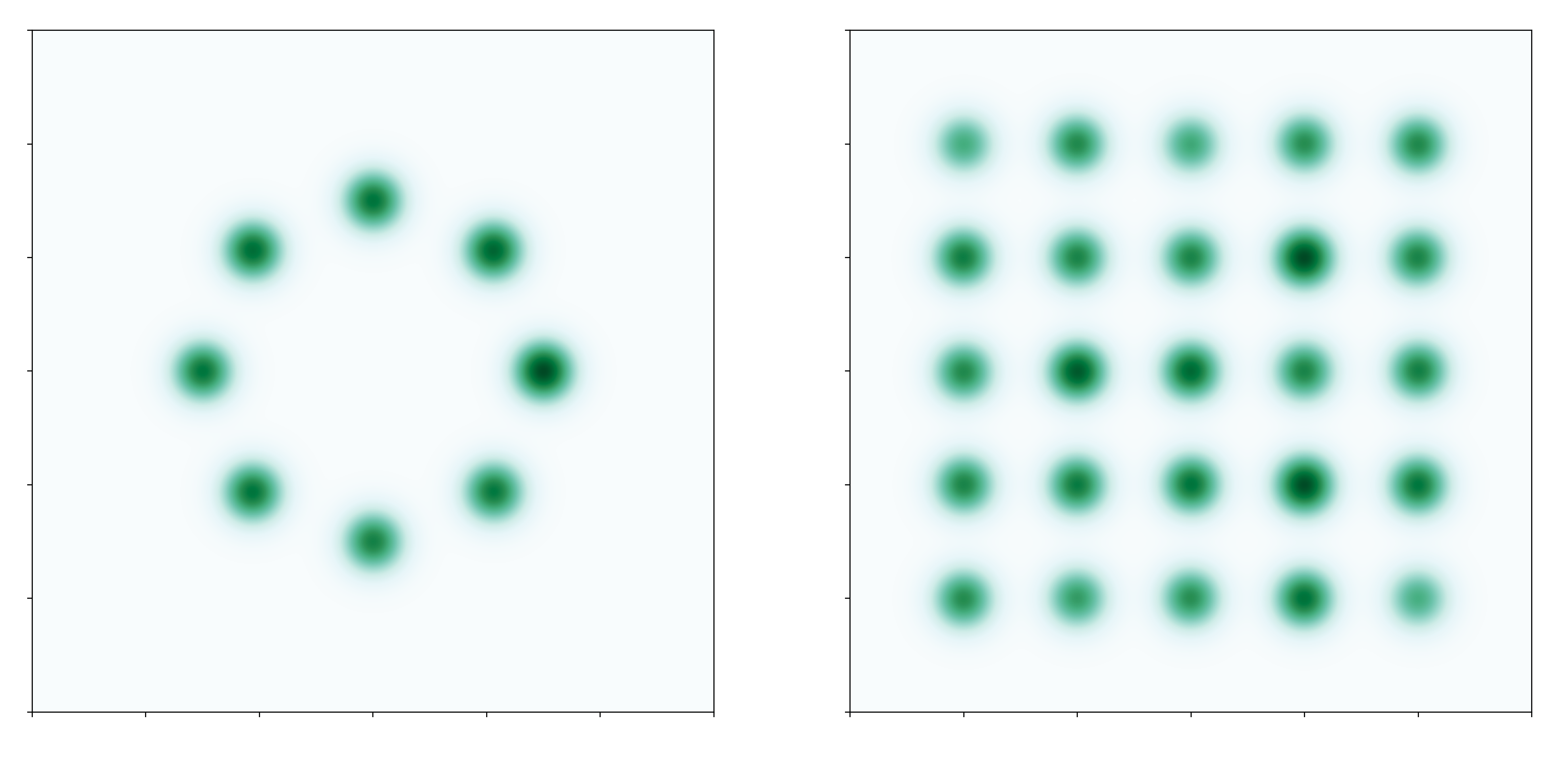
Figure 3: Real samples from the respective datasets. The image on the left represents samples from the Gaussian mixture with 8 components arranged on a ring, and the image on the right shows samples from the Gaussian mixture with 25 components arranged on a grid.

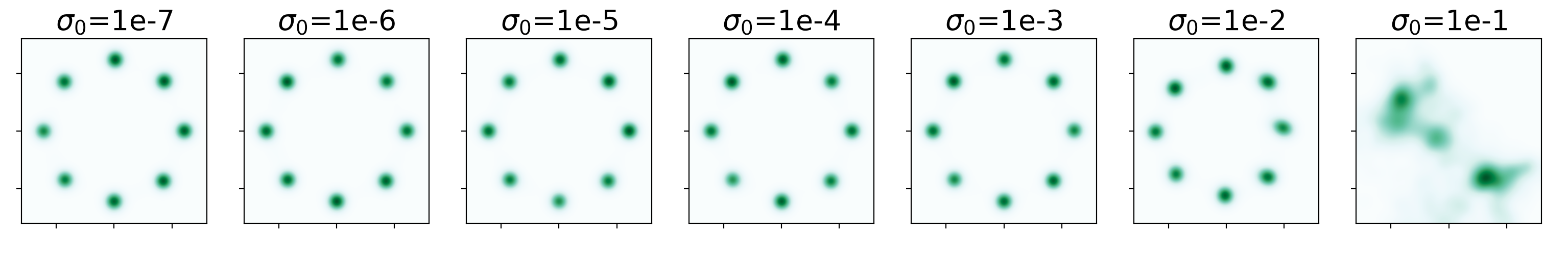
Figure 4: Samples from the models trained on the Gaussian ring

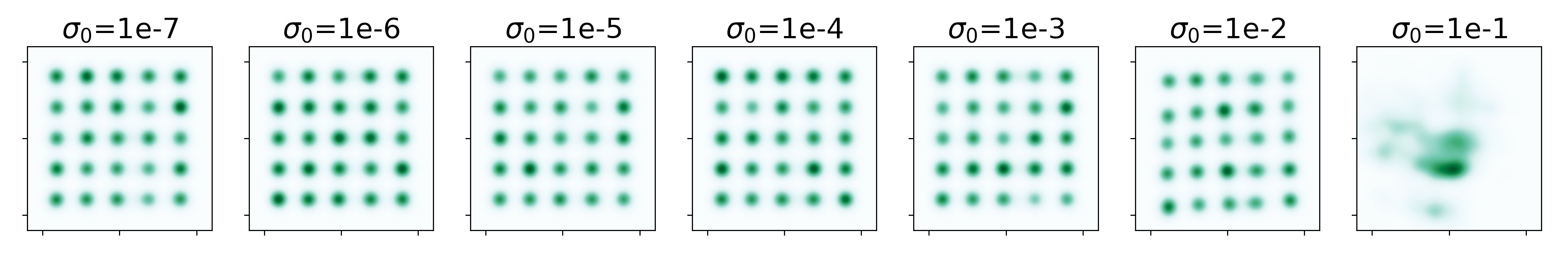
Figure 5: Samples from the models trained on the Gaussian grid

B.2 MNIST dataset

In our experiments with the MNIST dataset (Deng, 2012), we used the standard DCGAN architecture (Radford et al., 2016) for the generator and the critic. We experimented with different values for the hyperparameter $\sigma_{0}$ to train the probabilistic models. We computed the FID scores (Heusel et al., 2017) for the different models using $2000$ random samples and the off-the-shelf implementation provided in the Pytorch-ignite library (Fomin et al., 2020), with a inception network (Szegedy et al., 2016) pre-trained on Imagenet. Since the Inception network requires 3-channel images, we transformed the original MNIST images by copying the single channel twice. The scores obtained for different models are displayed in Table 1 and random (not cherry-picked) samples are displayed on Figures 7 to 11.

Table 1: FID scores from the various models trained on MNIST

$\sigma_{0}$	Score
$10^{-7}$	113.16
$10^{-6}$	106.59
$10^{-5}$	111.15
$10^{-4}$	107.54
$10^{-3}$	112.51
$10^{-2}$	189.30

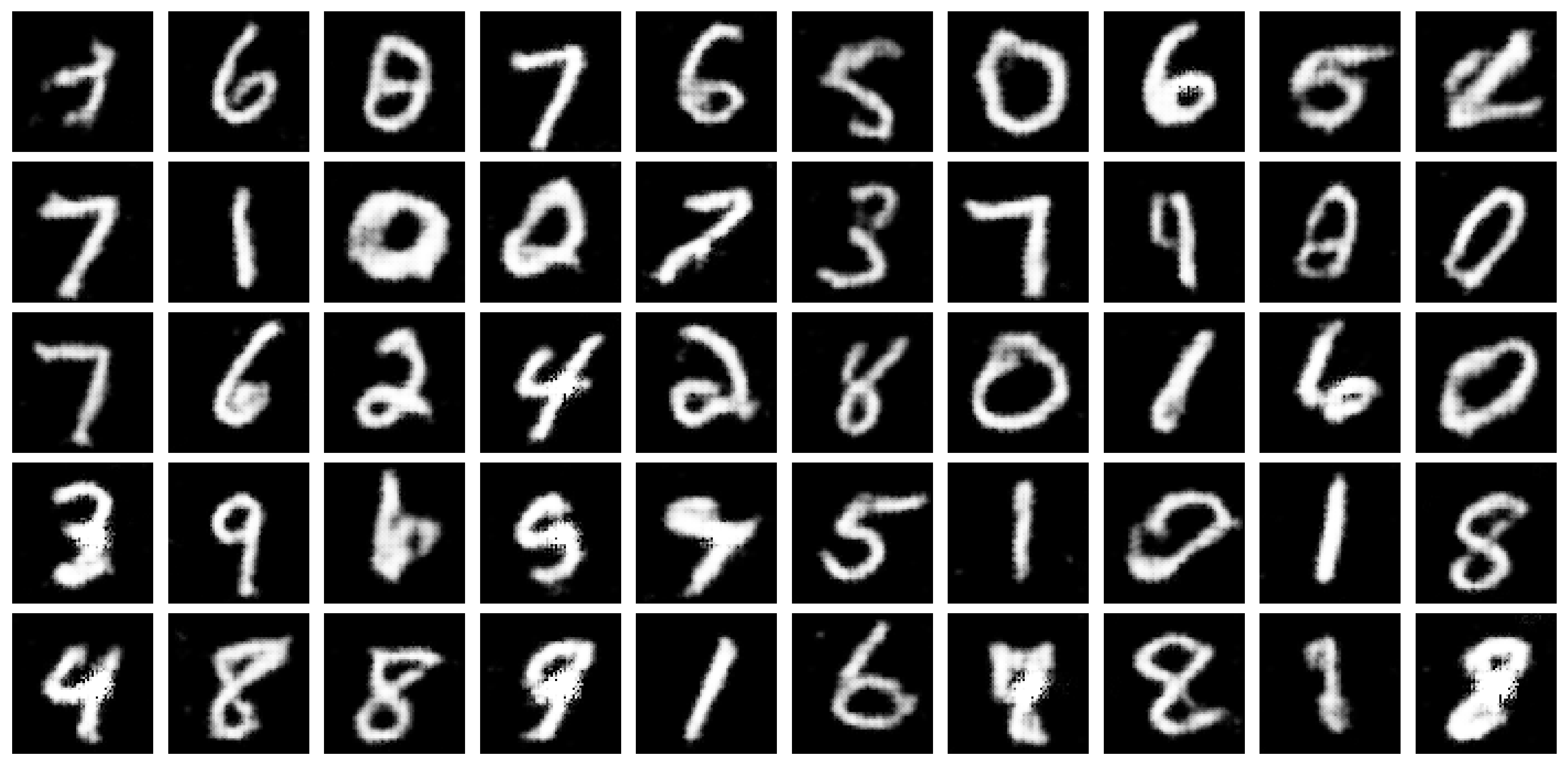
Figure 6: $\sigma_{0}=10^{-2}$

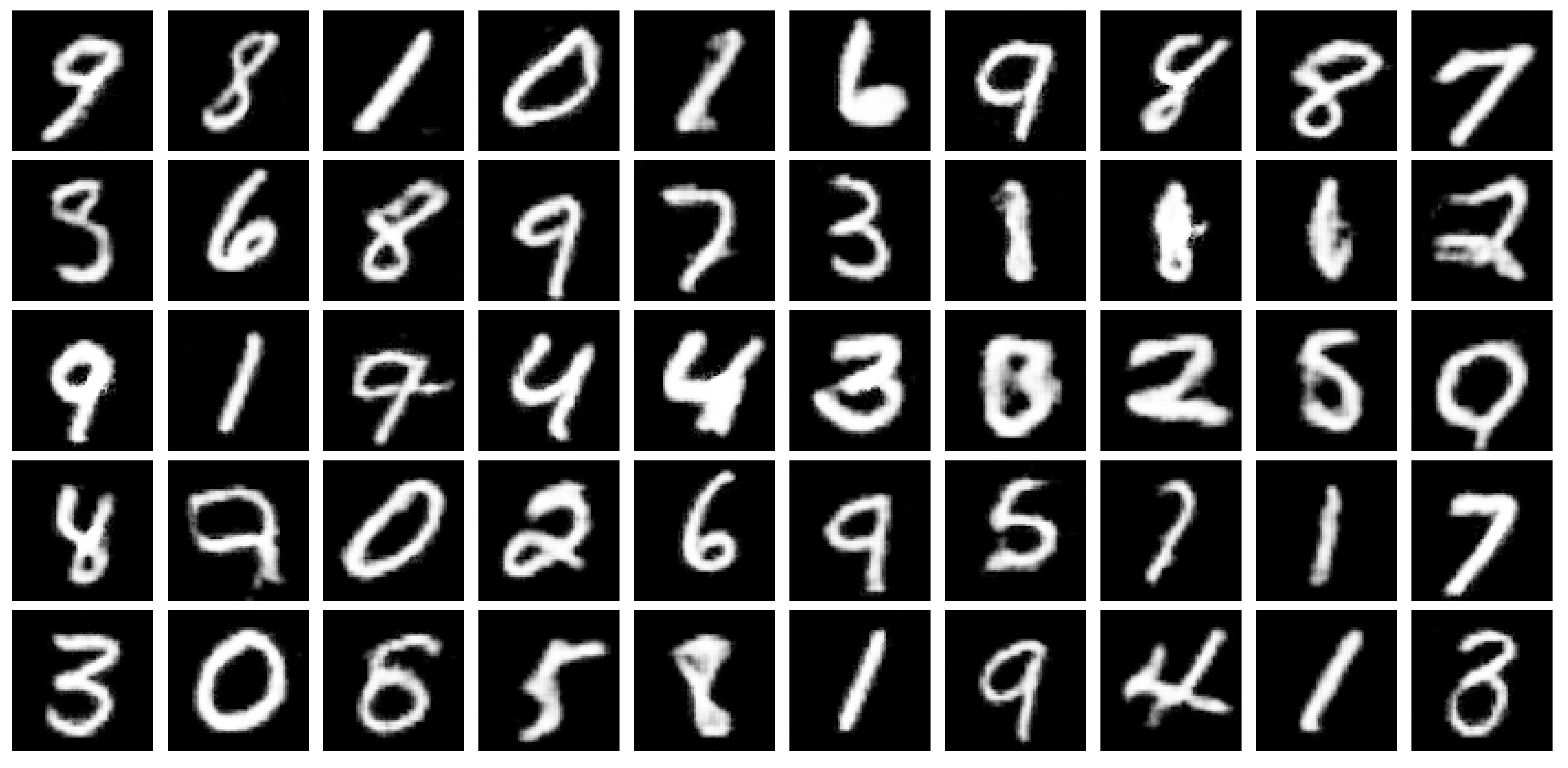
Figure 7: $\sigma_{0}=10^{-3}$

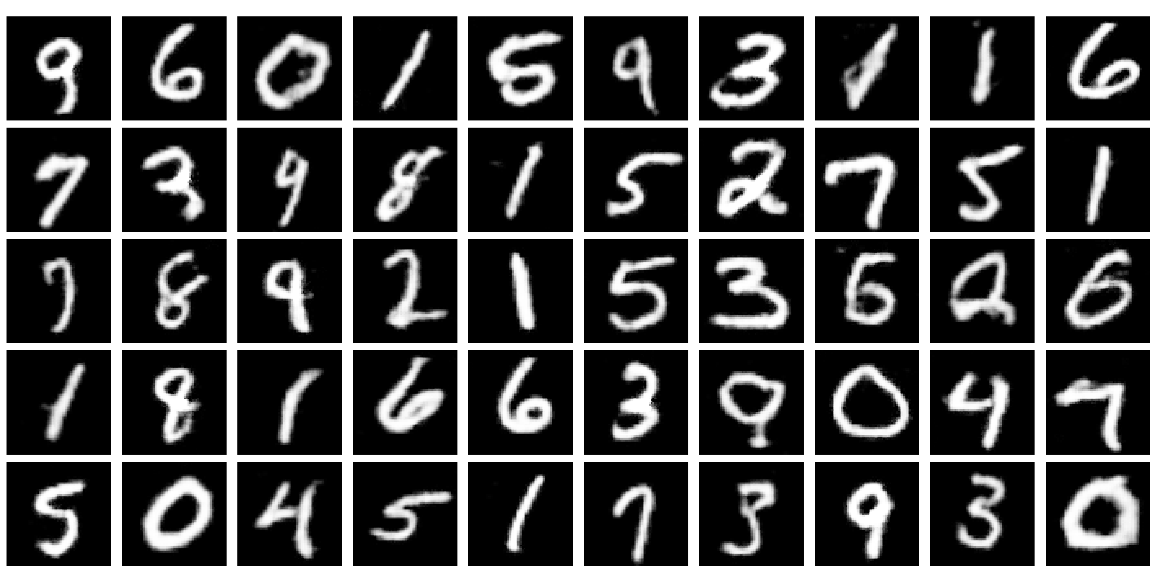
Figure 8: $\sigma_{0}=10^{-4}$

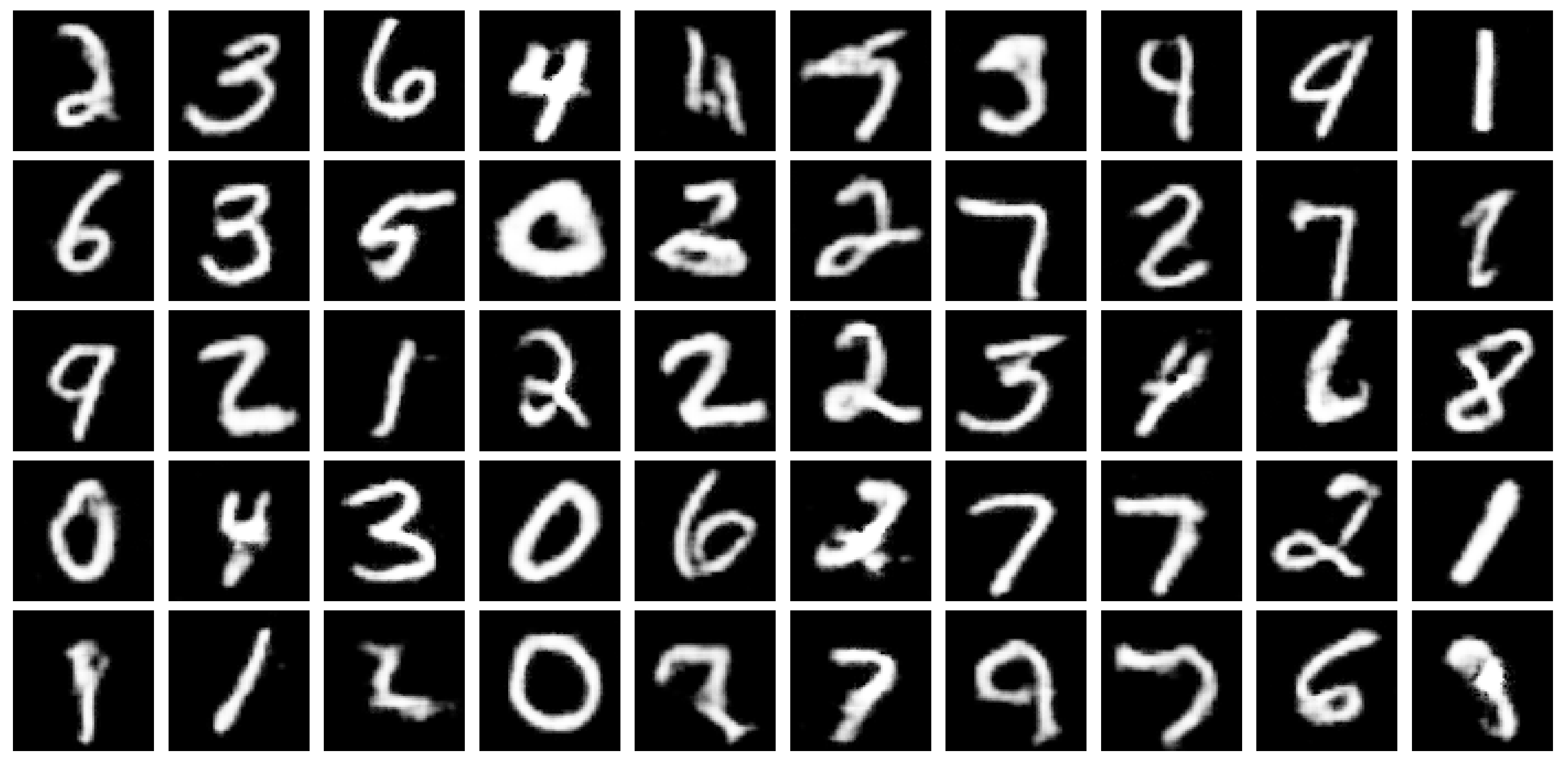
Figure 9: $\sigma_{0}=10^{-5}$

Figure 10: $\sigma_{0}=10^{-6}$

Figure 11: $\sigma_{0}=10^{-7}$

References

- Acharya et al. (2018) Acharya, D., Huang, Z., Paudel, D. P., and Van Gool, L. Towards high resolution video generation with progressive growing of sliced Wasserstein GANs. arXiv preprint arXiv:1810.02419, 2018.
- Alquier (2021) Alquier, P. User-friendly introduction to PAC-Bayes bounds. arXiv preprint arXiv:2110.11216, 2021.
- Amit & Meir (2018) Amit, R. and Meir, R. Meta-learning by adjusting priors based on extended PAC-Bayes theory. In International Conference on Machine Learning, pp. 205–214. PMLR, 2018.
- Amit et al. (2022) Amit, R., Epstein, B., Moran, S., and Meir, R. Integral probability metrics PAC-bayes bounds. In Advances in Neural Information Processing Systems, 2022.
- Anil et al. (2019) Anil, C., Lucas, J., and Grosse, R. Sorting out Lipschitz function approximation. In International Conference on Machine Learning, pp. 291–301. PMLR, 2019.
- Arjovsky et al. (2017) Arjovsky, M., Chintala, S., and Bottou, L. Wasserstein generative adversarial networks. In International Conference on Machine Learning, pp. 214–223. PMLR, 2017.
- Arora et al. (2017) Arora, S., Ge, R., Liang, Y., Ma, T., and Zhang, Y. Generalization and equilibrium in generative adversarial nets (GANs). In International Conference on Machine Learning, pp. 224–232. PMLR, 2017.
- Bégin et al. (2016) Bégin, L., Germain, P., Laviolette, F., and Roy, J.-F. PAC-Bayesian bounds based on the Rényi divergence. In International Conference on Artificial Intelligence and Statistics, pp. 435–444. PMLR, 2016.
- Biau et al. (2021) Biau, G., Sangnier, M., and Tanielian, U. Some theoretical insights into Wasserstein GANs. Journal of Machine Learning Research, 2021.
- Biggs & Guedj (2022) Biggs, F. and Guedj, B. On margins and derandomisation in PAC-Bayes. In International Conference on Artificial Intelligence and Statistics, pp. 3709–3731. PMLR, 2022.
- Björck & Bowie (1971) Björck, Å. and Bowie, C. An iterative algorithm for computing the best estimate of an orthogonal matrix. SIAM Journal on Numerical Analysis, 8(2):358–364, 1971.
- Borji (2019) Borji, A. Pros and cons of GAN evaluation measures. Computer Vision and Image Understanding, 179:41–65, 2019. ISSN 1077-3142.
- Brock et al. (2019) Brock, A., Donahue, J., and Simonyan, K. Large scale GAN training for high fidelity natural image synthesis. In International Conference on Learning Representations, 2019.
- Catoni (2007) Catoni, O. PAC-Bayesian supervised classification: the thermodynamics of statistical learning, volume 56. Institute of Mathematical Statistic, 2007.
- Chérief-Abdellatif & Alquier (2018) Chérief-Abdellatif, B.-E. and Alquier, P. Consistency of variational Bayes inference for estimation and model selection in mixtures. Electronic Journal of Statistics, 12(2):2995–3035, 2018.
- Chérief-Abdellatif et al. (2022) Chérief-Abdellatif, B.-E., Shi, Y., Doucet, A., and Guedj, B. On PAC-Bayesian reconstruction guarantees for VAEs. In International Conference on Artificial Intelligence and Statistics, pp. 3066–3079. PMLR, 2022.
- de Rosa & Papa (2021) de Rosa, G. H. and Papa, J. P. A survey on text generation using generative adversarial networks. Pattern Recognition, 119:108098, 2021.
- Deng (2012) Deng, L. The MNIST database of handwritten digit images for machine learning research. IEEE Signal Processing Magazine, 29(6):141–142, 2012.
- Dieng et al. (2019) Dieng, A. B., Ruiz, F. J., Blei, D. M., and Titsias, M. K. Prescribed generative adversarial networks. arXiv preprint arXiv:1910.04302, 2019.
- Dumoulin et al. (2017) Dumoulin, V., Belghazi, I., Poole, B., Lamb, A., Arjovsky, M., Mastropietro, O., and Courville, A. Adversarially learned inference. In International Conference on Learning Representations, 2017.
- Dziugaite & Roy (2018) Dziugaite, G. K. and Roy, D. M. Data-dependent PAC-Bayes priors via differential privacy. In Advances in Neural Information Processing Systems, volume 31, 2018.
- Fefferman et al. (2016) Fefferman, C., Mitter, S., and Narayanan, H. Testing the manifold hypothesis. Journal of the American Mathematical Society, 29(4):983–1049, 2016.
- Fodor (2002) Fodor, I. K. A survey of dimension reduction techniques. Technical report, Lawrence Livermore National Lab., CA (US), 2002.
- Fomin et al. (2020) Fomin, V., Anmol, J., Desroziers, S., Kriss, J., and Tejani, A. High-level library to help with training neural networks in pytorch. https://github.com/pytorch/ignite, 2020.
- Frid-Adar et al. (2018) Frid-Adar, M., Diamant, I., Klang, E., Amitai, M., Goldberger, J., and Greenspan, H. GAN-based synthetic medical image augmentation for increased CNN performance in liver lesion classification. Neurocomputing, 321:321–331, 2018.
- Germain et al. (2009) Germain, P., Lacasse, A., Laviolette, F., and Marchand, M. PAC-Bayesian learning of linear classifiers. In International Conference on Machine Learning, pp. 353–360, 2009.
- Germain et al. (2016) Germain, P., Bach, F., Lacoste, A., and Lacoste-Julien, S. PAC-Bayesian theory meets Bayesian inference. In Advances in Neural Information Processing Systems, volume 29, 2016.
- Goodfellow et al. (2014) Goodfellow, I., Pouget-Abadie, J., Mirza, M., Xu, B., Warde-Farley, D., Ozair, S., Courville, A., and Bengio, Y. Generative adversarial nets. In Advances in Neural Information Processing Systems, volume 27, 2014.
- Guedj (2019) Guedj, B. A primer on PAC-Bayesian learning. In Proceedings of the French Mathematical Society, volume 33, pp. 391–414. Société Mathématique de France, 2019.
- Gulrajani et al. (2017) Gulrajani, I., Ahmed, F., Arjovsky, M., Dumoulin, V., and Courville, A. C. Improved training of Wasserstein GANs. In Advances in Neural Information Processing Systems, volume 30, 2017.
- Haddouche & Guedj (2022) Haddouche, M. and Guedj, B. Online PAC-Bayes learning. In Advances in Neural Information Processing Systems, 2022.
- Haddouche et al. (2021) Haddouche, M., Guedj, B., Rivasplata, O., and Shawe-Taylor, J. PAC-Bayes unleashed: Generalisation bounds with unbounded losses. Entropy, 23(10), 2021.
- Heusel et al. (2017) Heusel, M., Ramsauer, H., Unterthiner, T., Nessler, B., and Hochreiter, S. Gans trained by a two time-scale update rule converge to a local nash equilibrium. In Advances in Neural Information Processing Systems, volume 30, 2017.
- Karras et al. (2019) Karras, T., Laine, S., and Aila, T. A style-based generator architecture for generative adversarial networks. In Proceedings of the IEEE/CVF conference on computer vision and pattern recognition, pp. 4401–4410, 2019.
- Kingma & Welling (2014) Kingma, D. P. and Welling, M. Auto-encoding Variational Bayes. In International Conference on Learning Representations, 2014.
- Langford & Caruana (2001) Langford, J. and Caruana, R. (not) bounding the true error. In Advances in Neural Information Processing Systems, volume 14, 2001.
- Liang (2021) Liang, T. How well generative adversarial networks learn distributions. Journal of Machine Learning Research, 22(228):1–41, 2021.
- McAllester (1999) McAllester, D. A. Some PAC-Bayesian theorems. Machine Learning, 37(3):355–363, 1999.
- McAllester (2003) McAllester, D. A. PAC-Bayesian stochastic model selection. Machine Learning, 51(1):5–21, 2003.
- McDiarmid (1989) McDiarmid, C. On the method of bounded differences, pp. 148–188. London Mathematical Society Lecture Note Series. Cambridge University Press, 1989.
- Müller (1997) Müller, A. Integral probability metrics and their generating classes of functions. Advances in Applied Probability, 29(2):429–443, 1997.
- Nagarajan & Kolter (2019) Nagarajan, V. and Kolter, J. Z. Uniform convergence may be unable to explain generalization in deep learning. In Advances in Neural Information Processing Systems, volume 32, 2019.
- Narayanan & Mitter (2010) Narayanan, H. and Mitter, S. Sample complexity of testing the manifold hypothesis. In Advances in Neural Information Processing Systems, volume 23, 2010.
- Neyshabur et al. (2018) Neyshabur, B., Bhojanapalli, S., and Srebro, N. A PAC-bayesian approach to spectrally-normalized margin bounds for neural networks. In International Conference on Learning Representations, 2018.
- Nguyen et al. (2021) Nguyen, K., Ho, N., Pham, T., and Bui, H. Distributional sliced-wasserstein and applications to generative modeling. In International Conference on Learning Representations, 2021.
- Ohana et al. (2022) Ohana, R., Nadjahi, K., Rakotomamonjy, A., and Ralaivola, L. Shedding a PAC-Bayesian light on adaptive sliced-Wasserstein distances. arXiv preprint arXiv:2206.03230, 2022.
- Parrado-Hernández et al. (2012) Parrado-Hernández, E., Ambroladze, A., Shawe-Taylor, J., and Sun, S. PAC-Bayes bounds with data dependent priors. Journal of Machine Learning Research, 13(1):3507–3531, 2012.
- Pérez-Ortiz et al. (2021) Pérez-Ortiz, M., Rivasplata, O., Shawe-Taylor, J., and Szepesvári, C. Tighter risk certificates for neural networks. Journal of Machine Learning Research, 22, 2021.
- Pope et al. (2021) Pope, P., Zhu, C., Abdelkader, A., Goldblum, M., and Goldstein, T. The intrinsic dimension of images and its impact on learning. In International Conference on Learning Representations, 2021.
- Rabin et al. (2011) Rabin, J., Peyré, G., Delon, J., and Bernot, M. Wasserstein barycenter and its application to texture mixing. In International Conference on Scale Space and Variational Methods in Computer Vision, pp. 435–446. Springer, 2011.
- Radford et al. (2016) Radford, A., Metz, L., and Chintala, S. Unsupervised representation learning with deep convolutional generative adversarial networks. In International Conference on Learning Representations, 2016.
- Repecka et al. (2021) Repecka, D., Jauniskis, V., Karpus, L., Rembeza, E., Rokaitis, I., Zrimec, J., Poviloniene, S., Laurynenas, A., Viknander, S., Abuajwa, W., et al. Expanding functional protein sequence spaces using generative adversarial networks. Nature Machine Intelligence, 3(4):324–333, 2021.
- Rezende et al. (2014) Rezende, D. J., Mohamed, S., and Wierstra, D. Stochastic backpropagation and approximate inference in deep generative models. In International Conference on Machine Learning, pp. 1278–1286. PMLR, 2014.
- Rivasplata et al. (2020) Rivasplata, O., Kuzborskij, I., Szepesvári, C., and Shawe-Taylor, J. PAC-Bayes analysis beyond the usual bounds. In Advances in Neural Information Processing Systems, volume 33, pp. 16833–16845, 2020.
- Salimans et al. (2016) Salimans, T., Goodfellow, I., Zaremba, W., Cheung, V., Radford, A., Chen, X., and Chen, X. Improved techniques for training GANs. In Advances in Neural Information Processing Systems, volume 29, 2016.
- Sandfort et al. (2019) Sandfort, V., Yan, K., Pickhardt, P. J., and Summers, R. M. Data augmentation using generative adversarial networks (cyclegan) to improve generalizability in ct segmentation tasks. Scientific reports, 9(1):1–9, 2019.
- Schreuder et al. (2021) Schreuder, N., Brunel, V.-E., and Dalalyan, A. Statistical guarantees for generative models without domination. In Algorithmic Learning Theory, pp. 1051–1071. PMLR, 2021.
- Seddik et al. (2020) Seddik, M. E. A., Louart, C., Tamaazousti, M., and Couillet, R. Random matrix theory proves that deep learning representations of GAN-data behave as gaussian mixtures. In International Conference on Machine Learning, pp. 8573–8582. PMLR, 2020.
- Shalaeva et al. (2020) Shalaeva, V., Esfahani, A. F., Germain, P., and Petreczky, M. Improved PAC-Bayesian bounds for linear regression. In AAAI Conference on Artificial Intelligence, volume 34, pp. 5660–5667, 2020.
- Singh et al. (2018) Singh, S., Uppal, A., Li, B., Li, C.-L., Zaheer, M., and Póczos, B. Nonparametric density estimation under adversarial losses. In Advances in Neural Information Processing Systems, volume 31, 2018.
- Srivastava et al. (2017) Srivastava, A., Valkov, L., Russell, C., Gutmann, M. U., and Sutton, C. Veegan: Reducing mode collapse in GANs using implicit variational learning. In Advances in Neural Information Processing Systems, volume 30, 2017.
- Szegedy et al. (2016) Szegedy, C., Vanhoucke, V., Ioffe, S., Shlens, J., and Wojna, Z. Rethinking the inception architecture for computer vision. In Proceedings of the IEEE conference on computer vision and pattern recognition, pp. 2818–2826, 2016.
- Theis et al. (2016) Theis, L., van den Oord, A., and Bethge, M. A note on the evaluation of generative models. In International Conference on Learning Representations, 2016.
- Uppal et al. (2019) Uppal, A., Singh, S., and Póczos, B. Nonparametric density estimation & convergence rates for GANs under besov ipm losses. In Advances in Neural Information Processing Systems, volume 32, 2019.
- Viallard et al. (2021) Viallard, P., Germain, P., Habrard, A., and Morvant, E. A general framework for the disintegration of PAC-Bayesian bounds. arXiv preprint arXiv:2102.08649, 2021.
- Villani (2009) Villani, C. Optimal transport: old and new, volume 338. Springer, 2009.
- Wang et al. (2018) Wang, Y.-X., Girshick, R., Hebert, M., and Hariharan, B. Low-shot learning from imaginary data. In Proceedings of the IEEE conference on computer vision and pattern recognition, pp. 7278–7286, 2018.
- Weed & Bach (2019) Weed, J. and Bach, F. Sharp asymptotic and finite-sample rates of convergence of empirical measures in Wasserstein distance. Bernoulli, 25(4A):2620–2648, 2019.
- Ying (2004) Ying, Y. McDiarmid’s inequalities of Bernstein and Bennett forms. City University of Hong Kong, pp. 318, 2004.
- Zhang et al. (2018) Zhang, P., Liu, Q., Zhou, D., Xu, T., and He, X. On the discrimination-generalization tradeoff in GANs. In International Conference on Learning Representations, 2018.
- Zhang et al. (2022) Zhang, Y., Gupta, A., Saunshi, N., and Arora, S. On predicting generalization using GANs. In International Conference on Learning Representations, 2022.
- Zhao et al. (2017) Zhao, J., Mathieu, M., and LeCun, Y. Energy-based generative adversarial networks. In International Conference on Learning Representations, 2017.