Primordial Black Holes Dark Matter and Secondary Gravitational Waves from Warm Higgs-G Inflation

Abstract

We explore the role of dissipative effects during warm inflation leading to the small-scale enhancement of the power spectrum of curvature perturbations. In this paper, we specifically focus on non-canonical warm inflationary scenarios and study a model of warm Higgs-G inflation, in which the Standard Model Higgs boson drives inflation, with a Galileon-like non-linear kinetic term. We show that in the Galileon-dominated regime, the primordial power spectrum is strongly enhanced, leading to the formation of primordial black holes (PBH) with a wide range of the mass spectrum. Interestingly, PBHs in the asteroid mass window $\sim(10^{17}$ – $10^{23}$) g are generated in this model, which can explain the total abundance of the dark matter in the Universe. In our analysis, we also calculate the secondary gravitational waves (GW) sourced by these small-scale overdense fluctuations and find that the induced GW spectrum can be detected in the future GW detectors, such as LISA, BBO, DECIGO, etc. Our scenario thus provides a novel way of generating PBHs as dark matter and a detectable stochastic GW background from warm inflation. We also show that our scenario is consistent with the swampland and the trans-Planckian censorship conjectures and, thus, remains in the viable landscape of UV complete theories.

I Introduction

The inflationary paradigm Kazanas:1980tx ; Sato:1980yn ; Guth:1980zm ; Linde:1981mu of the early Universe successfully explains the observations of anisotropies in the cosmic microwave background (CMB) radiation and generates seed inhomogeneties for the large scale structure (LSS) formation Planck:2018jri (for reviews, see Baumann:2009ds ; Linde:2007fr ; Riotto:2002yw ; Tsujikawa:2003jp ). Despite its phenomenal success, the underlying particle physics model of inflation remains elusive to date Linde:2005ht . In the Standard Model (SM) of particle physics, the only scalar field is the Higgs boson, whose self-interactions are so strong that it can not act as an inflaton (a scalar field that drives inflation) in a minimal setup and thus, can not explain the cosmological observations. However, by extending it to a non-minimal configuration, one can construct a viable inflationary model within the SM (for a review, see Ref. Rubio:2018ogq ). This can be achieved, for example, by introducing a non-minimal coupling of the Higgs field to gravity Bezrukov:2007ep ; Barvinsky:2008ia ; Germani:2010gm , or with a non-canonical kinetic term of the Higgs field, such as in the $k$-inflation Armendariz-Picon:1999hyi , ghost condensate Arkani-Hamed:2003juy , and Dirac-Born-Infeld inflation Alishahiha:2004eh models.

One such construction with a general kinetic term and additional non-linear terms are the Galileon-like models whose Lagrangian can be written as

$$\mathcal{L}_{\phi}=K(\phi,X)-G(\phi,X)\Box\phi,$$ (1)

where $X=-\frac{1}{2}g^{\mu\nu}\partial_{\mu}\phi\partial_{\nu}\phi$ is the standard kinetic term of the Galileon field $\phi$, $K(\phi,X)=X-V(\phi)$ where $V(\phi)$ is the field potential, and $G(\phi,X)$ is an arbitrary function of $\phi,X$. This specific form of the non-linear kinetic term is special, as it does not lead to extra degrees of freedom or ghost instabilities and maintains the gravitational and scalar field equations at the second order Deffayet:2009wt ; Deffayet:2009mn ; Kobayashi:2011nu . The Galileon field is named so because it possesses a Galileon shift symmetry in the Minkowski spacetime. Phenomenologically, Galileon-type scalar fields have been extensively studied in the context of dark energy, modified gravity Chow:2009fm ; Silva:2009km ; Kobayashi:2009wr ; Kobayashi:2010wa ; Gannouji:2010au ; DeFelice:2010gb ; DeFelice:2010pv as well as inflation Kobayashi:2010cm ; Mizuno:2010ag ; Burrage:2010cu ; Creminelli:2010qf ; Ohashi:2012wf . In Ref. Kamada:2010qe , the authors explored Higgs inflation in the presence of Galileon-like non-linear derivative interactions and demonstrated that this model is compatible with cosmological observations. Also, the tensor-to-scalar ratio for this model was found to be within the sensitivity of future experiments, which can be used to discriminate it from the standard inflationary model with a canonical kinetic term. However, when the Galileon term dominates over the standard kinetic term in this model, the dynamics of reheating is modified. For large self-coupling $\lambda$, there is no oscillatory phase and moreover, the square of sound speed $c_{s}^{2}$ is negative during reheating, leading to instabilities of small-scale perturbations Ohashi:2012wf .

In order to alleviate this problem, the authors in Ref. Kamada:2013bia extended the Higgs Lagrangian with higher order kinetic terms to obtain $c_{s}^{2}>0$, thereby avoiding instabilities. Alternatively, this problem would not arise in the first place, if there is no separate reheating phase after inflation, as it could be in the case of warm inflation. This was explored by the authors in Refs. Motaharfar:2017dxh ; Herrera:2017qux ; Motaharfar:2018mni , and forms the basis of this paper.

Warm inflation Berera:1995wh ; Berera:1995ie ; Berera:1998px is a general description of inflation in which the dissipative effects during inflation play an important role in the inflationary dynamics. The basic idea of warm inflation is that the inflaton is sufficiently coupled with other fields, such that it dissipates its energy into them during its evolution, which leads to a thermal bath (with temperature $T$) in the Universe during the inflationary phase. Therefore, a separate reheating phase is not necessarily needed for particle production. For reviews on warm inflation, see Refs. Berera:2006xq ; Berera:2008ar ; Oyvind&nbspGron:2016zhz .

The background dynamics of the inflaton as well as its fluctuations are modified in warm inflation, therefore, the primordial power spectrum has distinct signatures on cosmological observables, as compared to cold inflation. For instance, the tensor-to-scalar ratio in warm inflation is lowered, thus certain models of cold inflation, although ruled out from Planck observations, could be viable models in the warm inflation description Visinelli:2016rhn ; Benetti:2016jhf ; Arya:2017zlb ; Arya:2018sgw ; Bastero-Gil:2017wwl . Warm inflationary models also predict unique non-Gaussian signatures that can be used to test these models Gupta:2002kn ; Moss:2011qc ; Bastero-Gil:2014raa ; Mirbabayi:2022cbt . As the inflationary dynamics is modified in warm inflation, the slow roll conditions which demand an extremely flat potential, are also relaxed in these models Berera:2004vm . Further, some warm inflation models can provide a unified description for inflation, dark matter, and/or dark energy Rosa:2018iff ; Rosa:2019jci ; Sa:2020fvn ; DAgostino:2021vvv . Another interesting aspect of warm inflation models is that they can also explain the baryon asymmetry of the Universe Bastero-Gil:2011clw ; Basak:2021cgk . Warm inflation studies also show that for some models with a large value of the dissipation parameter, the swampland conjectures can be satisfied, thus making them in agreement with a high energy theory Das:2018rpg ; Motaharfar:2018zyb . We will discuss this aspect of our model in detail in Section IV. Since all these features of warm inflation arise from the fundamental principles of a dissipating system, it is very crucial to study warm inflation to understand the physics of the early Universe.

Although the large scale imprints of warm inflation are well studied through the observations of the CMB anisotropies, the small scale features have recently acquired much attention. One of the novel probes of small scale physics of inflation is the formation and abundance of primordial black holes (PBH) zeldo:1966 ; Hawking:1971ei ; Carr:1974nx . In contrast to the astrophysical black holes, which are the end stages of a star, PBHs are primordial in origin and may form by different mechanisms, such as the collapse of overdense fluctuations Carr:1974nx ; Carr:1975qj , bubble collisions Hawking:1982ga , collapse of strings Hogan:1984zb , domain walls Caldwell:1996pt , etc. In order to produce PBHs by the gravitational collapse, the amplitude of primordial curvature power spectrum at small scales has to be $\sim\mathcal{O}(10^{-2})$. Such an enhancement by several orders can be achieved in different models, such as the hybrid inflation GarciaBellido:1996qt ; Bugaev:2011wy ; Clesse:2015wea , running-mass inflation Leach:2000ea ; Kohri:2007qn ; Drees:2011hb ; Motohashi:2017kbs , hilltop inflation Alabidi:2009bk , inflating curvaton Kohri:2012yw , axion curvaton inflation Kawasaki:2012wr ; Ando:2017veq , double inflation Kawasaki:1997ju , thermal inflation Dimopoulos:2019wew , single field inflation with a broken scale invariance Bringmann:2001yp , or by introducing an inflection point (plateau) in the potential Garcia-Bellido:2017mdw ; Ballesteros:2017fsr ; Germani:2017bcs ; Bhaumik:2019tvl , or bump/dip in the potential Mishra:2019pzq , running of the spectral index Drees:2011yz ; Kohri:2018qtx ; Ghosh:2022okj , suppression of the sound speed Ozsoy:2018flq ; Zhai:2022mpi or resonant instability Cai:2018tuh ; Zhou:2020kkf , etc. PBHs are crucial probes of the small scale features of the primordial power spectrum and hence different inflationary models Green:1997sz ; Josan:2009qn ; Carr:2009jm ; Sato-Polito:2019hws .

The abundance of PBHs is constrained through various observations, e.g. PBHs with mass $M_{PBH}<10^{15}$ g, would have evaporated by today, and thus their consequences on the Big-Bang nucleosynthesis (BBN) can provide constraints on their initial mass fraction. The PBHs with mass $M_{PBH}\lesssim 10^{9}$ g would completely evaporate by BBN, and therefore the bounds on their abundance are not very stringent. Recent studies show that such ultralight PBHs might induce interesting observational imprints such as an extra contribution to the dark radiation and dark relics Bhaumik:2022zdd . It is also possible that these PBHs may dominate the universe for a short duration before the radiation dominated epoch, and lead to a secondary resonant enhancement of the induced GWs Bhaumik:2020dor ; Bhaumik:2022pil . For PBHs with $M_{PBH}>10^{15}$ g, the constraints arise from their gravitational effects, like lensing, dynamical effects on interaction with astrophysical systems, LIGO/Virgo gravitational wave (GW) merger events, etc. (For details, see Refs. Sasaki:2018dmp ; Carr:2020gox ). Also, PBHs can constitute a significant or total fraction of the dark matter (DM) density in the mass window ($10^{17}-10^{23}$) g (see recent reviews Carr:2020xqk ; Green:2020jor ). Thus, PBHs are very important from the aspects of DM phenomenology. Further, as for PBH generation, the amplitude of scalar fluctuations at smaller scales is hugely enhanced, there is an inevitable GW spectrum sourced by these large density fluctuations Mollerach:2003nq ; Ananda:2006af ; Baumann:2007zm ; Kohri:2018awv , which can have interesting observational consequences in the future GW detectors.

Motivated by this, we investigated the small scale features of warm inflation in our earlier works Arya:2019wck ; Arya:2022xzc and considered minimally coupled single-field models with a canonical kinetic term. We explored the formation of PBHs and the scalar induced GW spectrum from a model of warm inflation in Refs. Arya:2019wck ; Arya:2022xzc . In our analysis, we found that for our model, the primordial power spectrum is red-tilted ($n_{s}<1$) for the CMB scales, but turns blue-tilted ($n_{s}>1$) at the small scales with a large amplitude. This generates PBHs of mass nearly $10^{3}$ g and an associated GW spectrum over the frequency range $(1-10^{6})$ Hz. Further, these tiny mass PBHs would have evaporated by today, but the calculated initial abundance of these PBHs favors the possibility that the Planck-mass remnants of these PBHs could constitute the total dark matter.

Similar analysis was performed in another theoretically interesting scalar warm little inflaton model Bastero-Gil:2021fac . In this model, the dissipation coefficient $\Upsilon$, which is a measure of the inflaton interactions with other fields, switches its behaviour from $\Upsilon\propto 1/T$ to $\Upsilon\propto T^{\kappa}$ ($\kappa>0$) as inflation proceeds. It is found that the very small scale modes grow sufficiently to generate PBHs of mass $\sim 10^{6}$ g and a GW spectrum peaked at frequency $(10^{5}-10^{6})$ Hz. More recently, the authors in Ref. Correa:2022ngq explain the full abundance of dark matter in the form of PBHs in mass range $(10^{17}-10^{22})$ g from a model of warm natural inflation. Another interesting study considering inflaton dissipation to be effective only for a few efolds, rather than for the full duration (as in warm inflation), was carried out recently in Ref. Ballesteros:2022hjk . By choosing the peak of the primordial power spectrum at some specific scales, PBH in the above mass range are constructed from this model that can explain the full dark matter abundance. Thus, a study of the dissipative effects during inflation leading to small scale features is crucial for understanding the physics of the early Universe and the dark matter.

All the above models of warm inflation considered a minimally coupled inflaton with a canonical kinetic term. In this study, we explore the effects of a non-canonical kinetic term in the evolution of warm inflationary models and consider the warm Higgs-G model for the formation of PBHs and the associated GW spectra. While the motivation of Refs. Motaharfar:2017dxh ; Motaharfar:2018mni was to explore the parameter space consistent with the large scale CMB observations, we focus on simultaneously explaining the CMB, as well as identifying the parameter space for the required abundance of PBHs as dark matter. The formation of PBH and secondary GW from G-inflation have also been motivated in the standard cold description, such as in Refs. Lin:2020goi ; Lin:2021vwc ; Gao:2020tsa ; Yi:2020cut ; Teimoori:2021pte .

We consider two cases of warm Higgs-G inflation models with a quartic Higgs potential and a dissipation coefficient with a linear dependence on temperature $\Upsilon(\phi,T)\propto T$. For the Galileon term we consider a general form $G(\phi,X)\propto\phi^{2p+1}X^{q}$ and work with two models characterised by ($p=0$, $q=1$) and ($p=1$, $q=1$). The presence of the dissipation term as well as the non-canonical kinetic term damp the inflaton evolution in these models. While PBHs could not be produced in this canonical warm inflationary setup, we find that in the non-canonical models in the presence of G-term as considered in our paper, the power spectrum is hugely enhanced at the small scales. As a result, PBHs over a wide mass range can be generated in our scenario, which includes the asteroid mass range $(10^{17}-10^{23}$) g, for which PBHs can constitute the full dark matter abundance. We further calculate the scalar induced GW spectrum associated with these PBHs and find that GW with peak frequency in the sensitivity limits of the forthcoming detectors, such as LISA, BBO, DECIGO, etc. are generated in our models. Thus, future detections or non-detections of GW would be a useful test to these inflationary models. Moreover, we find that these models are also consistent with the swampland and the TCC conjectures and thus, they belong to the viable landscape of UV complete theories.

This paper is organised as follows: We begin with an introduction to the basics of warm inflation in Section II. Then we describe the inflationary dynamics in warm-G inflation in Section III. We then introduce our warm Higgs-G inflation model in Section IV. After parameterizing it in terms of the model parameters and discussing the predictions with CMB observations and swampland conjectures, we discuss the theory of PBH formation and the associated scalar induced GW in Section V. Then we discuss the results of our model in Section VI and summarize the paper in Section VII.

II Basics of Warm Inflation

In warm inflation, one considers the dissipative processes during inflation based on the principles of non-equilibrium field theory for interacting quantum fields. The inflaton is assumed to be near-equilibrium and evolving slowly as compared to the microphysics timescales in the adiabatic approximation, see Refs. Gleiser:1993ea ; Berera:1998gx ; Berera:2007qm . The dissipation of the inflaton field to radiation remains active throughout the duration of inflation which naturally ends when either the energy density of the radiation bath becomes larger than that of the inflaton or the slow roll conditions no longer hold.

The equation of motion of the inflaton $\phi$ slowly rolling down a potential $V(\phi)$ during warm inflation is modified due to an additional dissipation term $\Upsilon\dot{\phi}$ arising from the inflaton coupling to other fields and is given as

$$\ddot{\phi}+3H\dot{\phi}+\Upsilon\dot{\phi}=-V_{,\phi}.$$ (2)

Here, an overdot denotes the derivatives with respect to cosmic time $t$, $H$ is the Hubble parameter and the subscript _,ϕ represents derivative with respect to $\phi$. The term $\Upsilon(\phi,T)$ is the dissipation coefficient which usually depends on $\phi$ and temperature of the Universe $T$. One can also rewrite Eq. (2) in terms of a dissipation parameter $Q\equiv\frac{\Upsilon}{3H}$, as

$$\ddot{\phi}+3H(1+Q)\dot{\phi}+V_{,\phi}=0.$$ (3)

Since $Q$ is dimensionless, $Q>1$ is usually called the strong dissipative regime while $Q<1$ is referred as the weak dissipative regime of warm inflation. Due to the inflaton dissipation, there is an energy transfer from the inflaton to the radiation component, given as

$$\dot{\rho}_{r}+4H\rho_{r}=\Upsilon{\dot{\phi}}^{2}~{}.$$ (4)

It is assumed that the radiation thermalizes quickly after being produced, thus, $\rho_{r}=\frac{\pi^{2}}{30}g_{*}T^{4}$, where $T$ is the temperature of the thermal bath and $g_{*}$ is the effective number of relativistic degrees of freedom present during warm inflation. Note that, the energy-momentum tensor associated with the inflaton and radiation are not individually conserved while the total energy-momentum tensor of the system remains conserved.

II.1 Slow roll approximation

To achieve an adequate duration of inflation, the potential of inflaton needs to be sufficiently flat, so that the slow roll conditions are satisfied. This is described in terms of the slow roll parameters,

$$\epsilon_{\phi}=\frac{M_{Pl}^{2}}{2}\,\left(\frac{V_{,\phi}}{V}\right)^{2},\hskip 28.45274pt\eta_{\phi}={M_{Pl}^{2}}\,\left(\frac{V_{,\phi\phi}}{V}\right)$$ (5)

where $M_{Pl}=\sqrt{\frac{1}{8\pi G_{N}}}\simeq 2.44\times 10^{18}$ GeV is the reduced Planck mass and $G_{N}$ is the gravitational constant. In addition, in warm inflation, there are other slow roll parameters Hall:2003zp ; Moss:2008yb

$$\beta_{\Upsilon}={M_{Pl}^{2}}\,\left(\frac{\Upsilon_{,\phi}\,V_{,\phi}}{\Upsilon\,V}\right),\hskip 14.22636ptb=\frac{TV_{,\phi T}}{V_{,\phi}}~{},\hskip 14.22636ptc=\frac{T\Upsilon_{,T}}{\Upsilon}.$$ (6)

Here the subscript _,T represents derivative with respect to $T$. These additional slow roll parameters are a measure of the field and temperature dependence of the inflaton potential and the dissipation coefficient. The stability analysis of warm inflationary solution leads to the following conditions Moss:2008yb

$$\epsilon_{\phi}\ll 1+Q,\hskip 22.76228pt|\eta_{\phi}|\ll 1+Q,\hskip 22.76228pt|\beta_{\Upsilon}|\ll 1+Q,\hskip 22.76228pt0<b\ll\frac{Q}{1+Q},\hskip 22.76228pt|c|\leq 4.$$ (7)

Note that, the conditions on the slow roll parameters $\epsilon_{\phi}$ and $\eta_{\phi}$ are weaker than the corresponding conditions for cold inflation. For large dissipation parameter $Q$, the upper limit on $\epsilon_{\phi}$ and $\eta_{\phi}$ is increased, and therefore, the $\eta$ problem is relaxed in warm inflation Berera:2004vm . The condition on $b$ implies that warm inflation is only feasible when the thermal corrections to the inflaton potential remain small.

In the slow roll approximation, we can neglect $\ddot{\phi}$ in Eq. (3), which gives

$$\dot{\phi}\approx\frac{-V_{,\phi}}{3H(1+Q)},$$ (8)

and since $\dot{\rho}_{r}$ is small in Eq. (4), we can approximate $\dot{\rho}_{r}\approx 0$ and obtain

$$\rho_{r}\approx\frac{\Upsilon}{4H}{\dot{\phi}}^{2}=\frac{3}{4}Q{\dot{\phi}}^{2},$$ (9)

which indicates that the radiation energy density is determined by the dissipation parameter, as expected.

II.2 Dissipation coefficient

The dissipation coefficient $\Upsilon(\phi,T)$ is determined by the microphysics of the coupled inflaton-radiation system, which includes the channel of the inflaton decay to radiation, its coupling strength with other fields, mass and multiplicities of the radiation fields with which inflaton couples, the temperature of the thermal bath, etc. Moss:2006gt ; BasteroGil:2010pb ; BasteroGil:2012cm . Depending on the form of the interaction Lagrangian, there arise different forms of the dissipation coefficient, as discussed in the literature (see, for instance, Refs. Berera:1998gx ; Bastero-Gil:2018yen ; Bastero-Gil:2019gao for a review on the various studies about the finite temperature quantum field theory calculations of the dissipation coefficient). For our purpose, we will use a dissipation coefficient, which is linearly proportional to the temperature of thermal bath, i.e. $\Upsilon(\phi,T)\propto T.$ This particular form arises in a supersymmetric warm inflation model wherein the inflaton undergoes a two-stage decay mechanism via an intermediate field into radiation fields Moss:2006gt . In the high temperature limit, when the mass of the intermediate field is smaller than the temperature of thermal bath, one gets the above expression of dissipation coefficient. Also, this form of dissipation coefficient arises in the “Little Higgs” models of electroweak symmetry breaking with Higgs as psuedo-Nambu Goldstone boson of a broken $U(1)$ gauge symmetry Bastero-Gil:2016qru . For this work, we do not specify any particular microphysical description for the interaction Lagrangian and choose to work with the form $\Upsilon\propto T$. This form of dissipation coefficient has been previously considered in different warm inflation models in the context of CMB observations Benetti:2016jhf ; Bastero-Gil:2017wwl ; Arya:2018sgw . In this paper, we are interested in the small scale imprints arising from this form of the dissipation coefficient.

III Warm G-inflation

In this model, the inflaton also has a non-minimal kinetic term in the Lagrangian, as shown in Eq. (1). By the definition of warm inflation, the inflaton couples to radiation fields and dissipates its energy into them. The full action including the interaction and the radiation Lagrangian is given as,

$$\mathcal{S}=\int d^{4}x\sqrt{-g}\left[\frac{M_{Pl}^{2}}{2}R+X-V(\phi,T)-G(\phi,X)\Box\phi+\mathcal{L}_{r}+\mathcal{L}_{int}\right].$$ (10)

As mentioned before, $X$ is the standard kinetic term, $G(\phi,X)\Box\phi$ is the Galileon-like non-linear kinetic term with $G(\phi,X)$ an arbitrary function of $\phi$, $X$. Here $V(\phi,T)$ is the field and temperature dependent inflaton potential, $\mathcal{L}_{r}$ is the Lagrangian for radiation fields and $\mathcal{L}_{int}$ is the interaction Lagrangian for the inflaton and the fields into which it dissipates its energy. The radiation energy density remains subdominant than that of the inflaton during the inflationary phase.

By varying the action in Eq. (10) with respect to the metric, one obtains the components of stress-energy momentum tensor for the inflaton as Kobayashi:2010cm ; Motaharfar:2017dxh

$$\rho_{\phi} = X+V(\phi,T)+6HG_{,X}X\dot{\phi}-2G_{,\phi}X,$$ (11)

$$p_{\phi} = X-V(\phi,T)-2(G_{,\phi}+G_{,X}\ddot{\phi})X,$$ (12)

where $G_{,\phi}=\partial{G}/\partial{\phi}$, and $G_{,X}=\partial{G}/\partial{X}$. Also, due to the presence of Galileon-like non-minimal kinetic term, the Klein-Gordon equation for the inflaton gets modified as PhysRevD.96.103541,

$$\mathcal{B}\ddot{\phi}(t)+3H\mathcal{A}\dot{\phi}(t)+V_{,\phi}(\phi,T)=0,$$ (13)

with

$$\mathcal{B}=1+6HG_{,X}\dot{\phi}+6HG_{,XX}X\dot{\phi}-2G_{,\phi}-2G_{,X\phi}X,$$ (14)

and

$$\mathcal{A}=1+Q+3HG_{,X}\dot{\phi}+\frac{\dot{H}\dot{\phi}G_{,X}}{H}-2G_{,\phi}+2G_{,X\phi}X-\frac{G_{,\phi\phi}\dot{\phi}}{3H}.$$ (15)

In the limit, $G\to 0$ in Eq. (13), one recovers the warm inflation scenario in a minimal setup, as given in Eq. (2). From Eq. (13), (3), we see that both the dissipation and the Galileon interaction terms contribute as a damping term that further slows down the inflaton evolution. However, the radiation energy density evolves in the same way as in Eq. (4).

III.1 Slow roll conditions

In warm G-inflation, apart from the slow roll parameters given in Eqs. (5) and (6), one also has the following dimensionless parameters Motaharfar:2017dxh

$$\delta_{X}=\frac{X}{M_{Pl}^{2}H^{2}},\hskip 28.45274pt\delta_{GX}=\frac{\dot{\phi}XG_{,X}}{M_{Pl}^{2}H},\hskip 28.45274pt\delta_{G\phi}=\frac{XG_{,\phi}}{M_{Pl}^{2}H^{2}}.$$ (16)

The requirement of slow roll during inflation demands the validity of the following conditions, as shown in Ref. Motaharfar:2017dxh

$$|\epsilon_{\phi}|,|\eta_{\phi}|,|\beta_{\Upsilon}|\ll\mathcal{A},\hskip 17.07182pt|\delta_{X}|,|\delta_{GX}|,|\delta_{G\phi}|\ll 1,\hskip 17.07182pt0<b\ll\frac{Q}{\mathcal{A}},\hskip 17.07182pt|c|\leq 4,\hskip 17.07182pt|G_{,\phi}|=\frac{\delta_{G\phi}}{\delta_{X}}\ll 1.$$ (17)

In the slow roll approximation, $\dot{H},G_{,\phi},G_{,X\phi},G_{\phi\phi}$ terms are small, and thus Eqs. (14) and (15) can be approximated as

$$\mathcal{B}\approx 1+6HG_{,X}\dot{\phi}+6HG_{,XX}X\dot{\phi}.$$ (18)

$$\mathcal{A}\approx 1+Q+3HG_{,X}\dot{\phi}.$$ (19)

Moreover, the contribution of $\ddot{\phi}$ is negligible in the slow roll approximation, thus Eq. (13) can be written as

$$3H\mathcal{A}\dot{\phi}(t)+V_{,\phi}\simeq 0.$$ (20)

Also, the radiation energy density does not evolve much during the slow roll, thus Eq. (4) is approximated as

$$\rho_{r}\approx\frac{3}{4}Q{\dot{\phi}}^{2}.$$ (21)

Next, one can define an effective Galileon dissipation parameter as

$$Q_{G}\equiv Q/\mathcal{B}$$

and from Eqs. (20) and (21), obtain

$$3H\mathcal{B}\dot{\phi}\left(Q_{G}+\frac{\delta_{X}+3\delta_{GX}}{\delta_{X}+6(\kappa_{X}+1)\delta_{GX}}\right)+V_{,\phi}\simeq 0$$ (22)

where $\kappa_{X}=\frac{XG_{,XX}}{G_{,X}}$, and

$$\rho_{R}=C_{R}T^{4}\approx\frac{3}{4}\mathcal{B}Q_{G}{\dot{\phi}}^{2}$$ (23)

where $C_{R}=\frac{\pi^{2}}{30}g_{*}.$ When the G-term dominates the evolution, i.e., $|\delta_{X}|\ll|\delta_{GX}|$, then Eq. (22) becomes

$$3H\mathcal{B}\dot{\phi}\left(Q_{G}+\frac{1}{2(\kappa_{X}+1)}\right)+V_{,\phi}\simeq 0.$$ (24)

This equation governs the dynamics of the inflaton field during warm G-inflation.

III.2 Primordial Power Spectrum

Due to the presence of non-zero temperature during warm inflation, the primordial curvature power spectrum is dominantly sourced by the thermal fluctuations Hall:2003zp ; Graham:2009bf ; Ramos:2013nsa . The inflaton fluctuations are obtained by solving the stochastic Langevin equation sourced by thermal noise in the radiation bath. The intensity of noise depends on the dissipation coefficient through the fluctuation-dissipation theorem Gleiser:1993ea ; Berera:1998gx ; Berera:2007qm . When the dissipation coefficient has a temperature dependence $(\Upsilon\propto T^{c}$), the radiation fluctuations also couple to the inflaton fluctuations and leads to a growth in the power spectrum for $c>0$ Graham:2009bf . Following the calculation for warm inflation of Ref. Graham:2009bf , the power spectrum for warm G-inflation model has been calculated in Ref. Motaharfar:2018mni , and is given as

$$\Delta^{2}_{\mathcal{R}}|_{c_{s}k=aH}=\left(\frac{\sqrt{3}H^{3}T\sqrt{1+Q_{G}}}{4\pi\sqrt{\pi}c_{s}\dot{\phi}^{2}}\right)\left(1+\frac{Q_{G}}{Q_{c}}\right)^{3c}.$$ (25)

Here the first bracketed term corresponds to the case when there is no coupling of radiation fluctuations to the inflaton fluctuations, i.e. there is no temperature dependence in $\Upsilon$ ($c=0$). The term $\left(1+\frac{Q_{G}}{Q_{c}}\right)^{3c}$ represents the growth factor, and for a fixed $c$ and $Q_{G}$, it varies inversely to $Q_{c}$. While if we fix $c$ and $Q_{c}$, the behaviour of growth factor is directly proportional to value of $Q_{G}$. In the above expression, the effective sound speed $c_{s}$ is obtained from

$$c_{s}^{2}=\frac{\delta_{X}+4\delta_{GX}}{\delta_{X}+6(\kappa_{X}+1)\delta_{GX}}$$ (26)

and the factor $Q_{c}$ is given as

$$Q_{c}=\left(\left[\frac{G^{3,1}_{1,3}\left(\frac{1}{12c_{s}^{2}}|^{\hskip 17.07182pt1-3c/2\hskip 5.69046pt}_{2-c/2,\hskip 5.69046pt0,\hskip 5.69046pt5/2}\right)}{2^{3c}\Gamma_{R}(\frac{3c}{2})\Gamma_{R}(\frac{3c}{2}+\frac{5}{2})\Gamma_{R}(2+c)}\right]\frac{\Gamma_{R}(3c+\frac{3}{2})}{\Gamma_{R}(\frac{3}{2})}\right)^{-\frac{1}{3c}}$$ (27)

where $G^{3,1}_{1,3}$ is the Meijer-G function, and $\Gamma_{R}$ refers to the Gamma function. From this expression, we can see that $Q_{c}$ is inversely proportional to $c_{s}$. As $c_{s}$ decreases, $Q_{c}$ increases, which in turn makes the growth weaker, and vice-versa. We also stress the importance of parameter $c$, which is a measure of temperature dependence in the dissipation coefficient, i.e. $\Upsilon\propto T^{c}$. For positive values, as we increase $c$, the growth factor increases. In the G-dominated regime ($|\delta_{X}|\ll|\delta_{GX}|$), Eq. (26) can be approximated as

$$c_{s}^{2}\approx\frac{2}{3(\kappa_{X}+1)}=\frac{2G_{,X}}{3(G_{,X}+XG_{,XX})}.$$ (28)

The effects of Galileon-like terms appears in modifying the sound speed and in the limit $G\rightarrow 0$, $c_{s}^{2}\rightarrow 1$, one recovers the canonical warm inflation. However, in this study, we are interested in the G-dominated regime and using the expression (25) for parameterizing the power spectrum in terms of model parameters.

The primordial power spectrum could also be damped because of the shear viscous pressure in the radiation Bastero-Gil:2011rva . This would lead to a modified expression of primordial power spectrum with a comparatively slower growth rate or even a total suppression of the growth caused by inflaton and radiation coupled fluctuations. However, in this work, we do not consider any such effects and it would be noteworthy to consider them in future studies.

IV Warm Higgs-G model

We will now describe the model we have considered in this study, warm Higgs-G inflation. As the name suggests, we have a Galileon-like non-minimal kinetic term to the Standard Model Higgs boson in a warm inflation setup. The action for Higgs-G in warm inflation is given from the Refs. Kamada:2010qe ; Kamada:2013bia ; Motaharfar:2018mni as

$$\mathcal{S}_{WHGI}=\int d^{4}x\sqrt{-g}\left[\frac{M_{Pl}^{2}}{2}R-|D_{\mu}\mathcal{H}|^{2}-\lambda(|\mathcal{H}|^{2}-v^{2})^{2}-\frac{2\mathcal{H}^{\dagger}}{M^{4}}D_{\mu}D^{\mu}\mathcal{H}|D_{\mu}\mathcal{H}|^{2}+\mathcal{L}_{r}+\mathcal{L}_{int}\right]$$ (29)

where $D_{\mu}$ is the covariant derivative with respect to the Standard Model gauge symmetry, $\mathcal{H}$ is the SM Higgs doublet, $M$ represents some mass parameter. Higgs inflation is driven by the neutral component of Higgs field $\phi$, which has a self-coupling constant $\lambda$ and the vacuum expectation value of Higgs after electroweak symmetry breaking, $v=246$ GeV. We will consider the scenario when $\phi\gg v$, in which case the simplified action is given by

$$\mathcal{S}_{WHGI}=\int d^{4}x\sqrt{-g}\left[\frac{M_{Pl}^{2}}{2}R+X-\frac{\lambda\phi^{4}}{4}-\frac{\phi X}{M^{4}}\Box\phi+\mathcal{L}_{r}+\mathcal{L}_{int}\right],$$ (30)

where we have approximated the Higgs potential as quartic potential,

$$V(\phi)\simeq\frac{\lambda\phi^{4}}{4}.$$ (31)

In this study, we would choose a general form of non-linear Galileon interaction term ($G(\phi,X)\Box\phi$ term in the Lagrangian) as Kamada:2013bia ; Motaharfar:2017dxh ; Deffayet:2010qz

$$G(\phi,X)=-\frac{\phi^{2p+1}X^{q}}{M^{4q+2p}}$$ (32)

where $p$ and $q$ are some positive integers. We consider two models with G-term as $-\frac{\phi X}{M^{4}}$ (for $p=0,q=1$) and $-\frac{\phi^{3}X}{M^{6}}$ (for $p=1,q=1$). For the warm inflation setup, we choose the interaction Lagrangian in inflaton-radiation system such that the dissipation coefficient is given by Moss:2006gt ; BasteroGil:2010pb ; Bastero-Gil:2016qru

$$\Upsilon(\phi,T)=C_{T}T.$$ (33)

As discussed before, this form of the dissipation coefficient is obtained in certain microphysical descriptions of warm inflation. The temperature dependence in the dissipation coefficient couples the inflaton fluctuations to the fluctuations in the radiation fields and leads to a growth function in the primordial power spectrum. Other well-motivated forms of temperature and field dependence in the dissipation coefficient are equally interesting to explore further.

IV.1 Evolution equations in warm Higgs-G inflation

Now, we will study the inflationary dynamics for our warm Higgs-G inflation model, focussing on the regime wherein the G-term dominates the inflaton evolution. We begin with parameterizing the primordial power spectrum in Eq. (25) in terms of model parameters. First, we write the Friedmann equation for our model when the inflaton potential dominates the energy density of the Universe, as

$$H^{2}\simeq\frac{\text{$\lambda$}}{12}\text{$M_{Pl}$}^{2}\left(\frac{\phi}{M_{Pl}}\right)^{4}.$$ (34)

Next, we want to evaluate $\dot{\phi}$. For this, we simplify Eq. (18) for our model and obtain

$$\mathcal{B}=-6Hq^{2}\dot{\phi}~{}\frac{\phi^{2p+1}X^{q-1}}{M^{4q+2p}}$$ (35)

where $X=-\frac{\dot{\phi}^{2}}{2}.$ Then by substituting the expression for $\mathcal{B}$ in Eq. (24), we get

$$\dot{\phi}=-M_{Pl}^{2}\zeta_{1}^{\frac{1}{2q}}\left(Q_{G}+\frac{1}{2q}\right)^{-\frac{1}{2q}}\left(\frac{\phi}{M_{Pl}}\right)^{-\frac{(p+1)}{q}},$$ (36)

where $\zeta_{1}=\frac{2^{q}}{3q^{2}}\left(\frac{M}{\text{$M_{Pl}$}}\right)^{2p+4q}$. We would further express the field evolution in terms of the parameter $Q_{G}$. From the form of dissipation coefficient in Eq. (33), and the definitions of $\Upsilon,Q,Q_{G}$, we can write $T=\frac{3H\mathcal{B}Q_{G}}{C_{T}}$, and then substitute it in Eq. (23). Then using Eq. (36), we get a relation between $\phi$ and $Q_{G}$ as

$$\frac{\phi}{M_{Pl}}=\left[\frac{\text{$Q_{G}^{3}$}\left(\frac{1}{2q}+\text{$Q_{G}$}\right)^{\frac{5-6q}{2q}}}{\text{$\zeta_{2}$}}\right]^{-\frac{q}{5p+11q+5}}.$$ (37)

Later, we also plot and discuss the total field excursion for different values of $Q_{G},p$ and $q$ in our warm inflation models in the context of swampland conjectures.

We next evaluate the expression for temperature of the thermal bath of radiation. Using Eqs. (23), (35) and (36), we get

$$\frac{T}{M_{Pl}}=Q_{G}^{\frac{1-3a}{4}}\left(\frac{1}{2q}+Q_{G}\right)^{\frac{2q(3a-1)-5a-1}{8q}}\left(\frac{\sqrt{3\lambda}}{2C_{R}}\zeta_{1}^{\frac{1}{2q}}\zeta_{2}^{a}\right)^{\frac{1}{4}}$$ (38)

where $\text{$\zeta_{2}$}=\frac{\sqrt{3}\text{$C_{T}^{4}$}}{2\text{$C_{R}$}\text{$\lambda$}^{7/2}}\text{$\zeta_{1}$}^{\frac{5}{2q}}$ and $a=\frac{-p+q-1}{5p+11q+5}$. Finally, with the Eqs. (34), (36), (37) and (38), we have parameterized the primordial power spectrum in terms of parameters $Q_{G}$, $\lambda$, $C_{T}$, $M$, $p,q$, and $c_{s}$ (which is a function of $p,q$). For a chosen model i.e. fixed $p,q$ (and $c_{s}$ accordingly), and a fixed $Q_{G}$ value at the pivot scale, we have three unknown parameters, $\lambda,C_{T},$ and $M$. The variable $Q_{G}$ is dynamical during inflation. We know that the end of warm inflation is determined from the equation $\epsilon_{H}=-\frac{\dot{H}}{H^{2}}=1$, which gives

$$\frac{1}{2\zeta_{3}}(Q_{G}^{end})^{-3b}\left(\frac{1}{2q}+Q_{G}^{end}\right)^{\frac{(6q-5)b+1}{2q}}=1.$$ (39)

where $\text{$\zeta_{3}$}=2\sqrt{\frac{3}{\text{$\lambda$}}}\text{$\zeta_{1}$}^{\frac{1}{2q}}\text{$\zeta_{2}$}^{-b}$ and $Q_{G}^{end}$ is the value of $Q_{G}$ at the end of inflation. Thus, for a warm inflation model with a fixed $\lambda$, the above equation gives a relation between $Q_{G}^{end}$, $C_{T}$ and $M$. But, since we also have $Q_{G}^{end}$ as unknown, we need to evaluate the evolution of $Q_{G}$ as a function of number of efolds $N_{e}$ for our warm inflation model. In our notation, we count the number of efolds from the end of inflation, i.e. $N_{end}=0$. From Eq. (37), we have a relation between $\phi$ and $Q_{G}$. On differentiating both sides with $N_{e}$ and using the fact that $dN_{e}=-Hdt$, we have $d\phi/dN_{e}=-\dot{\phi}/H$. On substituting for $\dot{\phi}$ from Eq. (36), we get

$$\frac{dQ_{G}}{dN_{e}}=-\zeta_{3}(22q+10p+10)\frac{Q_{G}^{3b+1}}{5Q_{G}+3}\left(\frac{1}{2q}+Q_{G}\right)^{-\frac{2q(3b-1)-5b+1}{2q}}$$ (40)

where $b=\frac{p+3q+1}{5p+11q+5}.$ We next integrate this equation from pivot scale till the end of inflation, to obtain $Q_{G}^{end}$, as

$$\zeta_{3}N_{e}=F(Q_{G}^{end})-F(Q_{G}^{P})$$ (41)

where

$$F(Q_{G})=-\frac{qQ_{G}^{-3b}\left(\frac{1}{2q}+Q_{G}\right)^{\frac{6bq-5b+1}{2q}}\left(5-\frac{{}_{2}F_{1}(1,\frac{1-5b}{2q};1-3b;-2qQ_{G})}{b}\right)}{(5b-1)(5p+11q+5)}.$$

With this relation, for a fixed number of efolds of inflation $N_{e}=50$ (or $60$) and a chosen value of $\lambda$ and $Q_{G}$ at the pivot scale ($Q_{G}^{P}$), we again obtain the $Q_{G}$ value at the end of inflation ($Q_{G}^{end}$) as a function of $C_{T}$ and $M$. Since we have three variables ($Q_{G}^{end},C_{T},M$) and two equations (39), (41), we need to provide an additional constraint to know these exactly. We use the normalisation of primordial power spectrum at the pivot scale ($k_{P}=0.05$ Mpc^-1) as $\Delta^{2}_{\mathcal{R}}(k_{P})=2.1\times 10^{-9}$ and therefore obtain the values of all the variables. In this way, we parameterize the power spectrum for our warm Higgs-G model in terms of model parameters and estimate their values compatible with the CMB observations.

IV.2 Constraints on warm Higgs-G inflation model from CMB

Here we show the results for different cases of our warm Higgs-G inflation model. We have chosen $\lambda=0.13$ (the largest value of Higgs self-coupling from quantum field theory) for our study. In all the plots, for each value of $Q_{G}$ (chosen at the pivot scale), we have a different set of $C_{T}$ and $M$ values that satisfy the normalisation condition for the primordial power. We consider the following set of values for $p$ and $q$.

Model I: $p=0,q=1$, which effectively represents the Galileon interaction term, $G=-\frac{\phi X}{M^{4}}$. For these values of $p,q$, the sound speed corresponds to $c_{s}=\sqrt{\frac{2}{3}}=0.816$. In this model, we first identify the parameter space of $Q_{G}$ values, which are consistent with the $n_{s}$ bounds from the Planck observations. For this, we plot the spectral index $n_{s}$ versus $Q_{G}$ value at the pivot scale in Fig. 1 for $50$ and $60$ efolds of inflation. The colored band in the Figure represents the Planck $2\sigma$ allowed range for the $n_{s}$. We obtain that for $N_{e}=50$, $10^{-0.98}\leq Q_{G}\leq 10^{-0.135}$ is consistent within the $n_{s}-2\sigma$ bounds, while for $N_{e}=60$, the allowed range is $10^{-0.68}\leq Q_{G}\leq 10^{-0.25}$. We can also see from the Figure that the spectrum is red-tilted ($n_{s}<1$) for small $Q_{G}$ values, while it tends to become blue-tilted ($n_{s}>1$) as $Q_{G}$ increases.

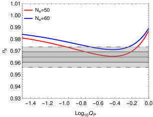
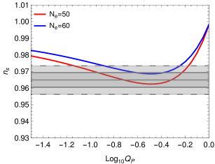
Figure 1: Plots of the spectral index $n_{s}$ vs. $Q_{P}$ (equal to the value of $Q_{G}$ at the pivot scale) for 50 (red) and 60 (blue) efolds of inflation for 1 Model I: $p=0,q=1$, and 1 Model II: $p=1,q=1$. The grey shaded bands represent the $1\sigma$ and $2\sigma$ allowed ranges from the Planck observations.

Model II: $p=1,q=1$, which effectively represents the Galileon interaction term, $G=-\frac{\phi^{3}X}{M^{6}}$. For these values of $p,q$ also, the sound speed $c_{s}=\sqrt{\frac{2}{3}}$. To estimate the range of $Q_{G}$ values consistent with the CMB, we plot the $n_{s}$ versus $Q_{G}$ value at the pivot scale for $50$ and $60$ efolds of inflation in Fig. 1. We obtain that for $N_{e}=50$, $10^{-1.14}\leq Q_{G}\leq 10^{-0.17}$ is consistent within the $n_{s}-2\sigma$ bounds, and for $N_{e}=60$, the allowed range is $10^{-0.88}\leq Q_{G}\leq 10^{-0.24}$. Also, the power spectrum is red-tilted at the large scales but turns blue tilted for the small scales. This is favorable for PBH production, which we will see in the next section.

IV.3 Swampland conjectures and our model

As inflation is described by a low energy effective field theory, it has to obey some criteria, such as the swampland and trans-Planckian censorship conjectures (TCC), in order to embed it in a UV complete theory, as follows Obied:2018sgi ; Kehagias:2018uem ; Kinney:2018nny ; Bedroya:2019snp :

• Distance conjecture: This criteria puts a limit on the scalar field range traversed during inflation, and is given as

  $$\frac{|\Delta\phi|}{M_{Pl}}\leq a$$ (42)

  where the constant $a\sim\mathcal{O}(1)$. This implies that small field models of cold inflation are more favorable than the large field models.

• de Sitter conjecture: This criteria gives a lower limit on the slope of inflationary potential as

  $$M_{Pl}\frac{|V_{,\phi}|}{V}\geq b$$ (43)

  where the constant $b\sim\mathcal{O}(1)$. This condition implies that the steep potentials are favorable for inflationary dynamics, which is not actually supported in the standard cold inflation in a minimal setup.

• Trans-Planckian Censorship conjecture (TCC): This criteria demands that the super-Planckian quantum fluctuations never become superhorizon during inflation, which sets a limit on the scale of inflation as Bedroya:2019tba

  $$V^{1/4}<3\times 10^{-10}M_{Pl}.$$ (44)

  This implies that the energy scale of inflation has to be lower than $\sim 10^{9}$ GeV to satisfy TCC bound. Such a low energy scale inflation yields a negligible amplitude of primordial gravitational waves and tensor-to-scalar ratio, $r<2.7\times 10^{-31}$.

It is extremely challenging to satisfy these conjectures in a single-field cold inflation model with a canonical kinetic term and a Bunch Davies vacuum, to embed them in a UV complete theory. However, if one extends to multifield inflation Achucarro:2018vey or curvaton models or by choosing different initial vaccuum state Ashoorioon:2018sqb or a non-canonical kinetic term, one can construct inflationary models compatible with the swampland distance and de Sitter conjectures Das:2018hqy ; Kehagias:2018uem .

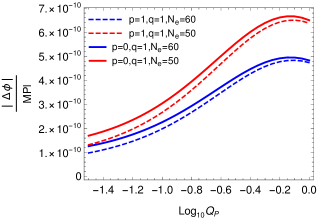
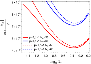
Figure 2: Plots of the field excursion $|\Delta\phi|$ (in units of $M_{Pl}$) and the slope of inflationary potentials $M_{Pl}\frac{|V_{,\phi}|}{V}$ vs. $Q_{P}$ for our warm inflation models. The solid (dashed) red and blue lines represent $50$ and $60$ efolds of inflation with Model I: $p=0,q=1$ (Model II: $p=1,q=1)$.

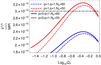
Figure 3: Plots of the scale of inflation $V^{1/4}$ (in units of $M_{Pl}$) and the tensor-to-scalar ratio $r$ vs. $Q_{P}$ for our warm inflation models. The solid (dashed) red and blue lines represent $50$ and $60$ efolds of inflation with Model I: $p=0,q=1$ (Model II: $p=1,q=1)$. The black dot-dashed lines represent the upper bound on both the quantities.

Contrary to the cold inflation, warm inflation is an interesting framework in which these conjectures could be satisfied due to the modified dynamics of inflaton field. There exists a few warm inflationary studies Das:2018rpg ; Motaharfar:2018zyb ; Kamali:2019xnt ; Das:2019acf ; Das:2020xmh ; Bertolami:2022knd ; Santos:2022exm in this context, which show that with a strong dissipation, the energy scale of inflation is sufficiently lowered, satisfying the above conjectures. Here we discuss the status of these conjectures for our warm Higgs-G model. In Fig. 2, we plot the field excursion $|\Delta\phi|/M_{Pl}$ and the slope of inflationary potential ${M_{Pl}}|V_{,\phi}|/V$ for our models with different $Q_{G}$ value at the pivot scale (denoted by $Q_{P}$). The solid (dashed) red and blue lines represent Model I (Model II) for $50$ and $60$ efolds of inflation, respectively. It is evident from the figure that the swampland distance and de-Sitter conjectures are in agreement with our models, implying that these models lie in the UV complete landscape theories of inflation. Further we plot the scale of inflation $V^{1/4}/M_{Pl}$ and the tensor-to-scalar ratio $r$ for our warm inflation models in Fig. 3. We find that both the TCC and the constraint on the tensor-to-scalar ratio are satisfied for these models with $60$ efolds of inflation, however for $50$ efolds, there is some parameter range of $Q_{P}$ which does not satisfactorily obey the bound.

To conclude, we have seen that for some parameter space of our warm inflation models, the CMB constraints on $n_{s}-r$ are well obeyed. Further, the swampland and TCC conjectures are also in agreement with these models, implying that they lie in the viable landscape theories of inflation. We next study the small scale features of these models in the context of formation of PBH.

V PBH formation and scalar induced gravitational waves

In the previous Section, we found that in our models, the primordial power spectrum is turning blue-tilted on the small scales and therefore can generate a significant abundance of PBHs, if the amplitude of the fluctuations is large. Further, these overdense perturbations also source the tensor perturbations and lead to secondary gravitational waves. In this Section, we will briefly discuss the PBH formation and the associated GW generation. For more detailed derivation, see Refs. Ananda:2006af ; Baumann:2007zm ; Kohri:2018awv ; Arya:2019wck ; Arya:2022xzc .

V.1 PBH formation

As mentioned before, PBHs can be produced via the collapse of large inhomogeneities generated during inflation. We consider that the PBHs are generated in the radiation-dominated era when fluctuations reenter the horizon. The mass of the generated PBHs is a fraction, $\gamma$ of the horizon mass at that epoch and is given as Green:1997sz

$$M_{PBH}(k)=\gamma\frac{4\pi}{3}\rho\left.H^{-3}\right|_{k=aH}.$$ (45)

where, $\rho$, $a$, and $H$ represents the energy density, scale factor and Hubble expansion rate at the time of PBH formation, respectively. Also, as different comoving fluctuation modes $k$ reenter the horizon at different epochs, the mass of the generated PBHs are given as,

$$M_{PBH}(k)\simeq 5\times 10^{15}{\rm{g}}\left(\frac{g_{*0}}{g_{*i}}\right)^{1/6}\left(\frac{10^{15}{\rm{Mpc}}^{-1}}{k}\right)^{2}$$ (46)

where $\Omega_{r0}$ is the present day radiation energy density fraction, $g_{*0}$ and $g_{*i}$ represent the relativistic degrees of freedom present in the Universe today and at the time of PBH formation, respectively. The fraction of the horizon mass collapsing into the PBHs is taken as $\gamma=0.2$ Carr:1975qj . From Eq. (46), we see that $M_{PBH}\propto k^{-2}$, which suggests that large (small) $k$ leads to small (large) mass PBHs. Further, an important quantity, known as the initial mass fraction of PBHs, $\beta(M_{PBH})$ is defined as

$$\beta(M_{PBH})=\frac{\rho_{{PBH},i}}{\rho_{total,i}}$$ (47)

where, $\rho_{{PBH},i}$ and $\rho_{total,i}$ are the energy density of PBHs and total energy density of the Universe at the time of PBH formation. Assuming that PBHs are formed in the radiation-dominated era, the expression of $\beta(M_{PBH})$ can be expressed in the form of present day observables as

$$\beta({M_{PBH}})= \frac{\Omega_{PBH,0}({M_{PBH}})}{\Omega_{r0}^{3/4}}\left(\frac{g_{*i}}{g_{*0}}\right)^{1/4}\left(\frac{M_{PBH}}{M_{0}}\right)^{1/2}\gamma^{-1/2}~{}~{}.$$ (48)

Here, $\Omega_{PBH,0}({M_{PBH}})=\rho_{{PBH},0}/\rho_{{crit},0}$ is the present day PBH energy density fraction, with $\rho_{{PBH},0}$ and $\rho_{{crit},0}$ representing the present energy density of PBHs and the critical energy density of the Universe, respectively.

The abundance of PBHs is theoretically obtained by the Press-Schechter theory Press:1973iz . For an overdense fluctuation reentering the horizon during a radiation-dominated era with an amplitude above a critical value $\delta_{c}$, the initial mass fraction of PBHs with mass $M_{\rm{PBH}}$ is given as Press:1973iz ,

$$\beta({M_{PBH}})= \frac{2}{\sqrt{2\pi}\sigma(R)}\int_{\delta_{c}}^{1}\exp\left(\frac{-\delta^{2}(R)}{2\sigma^{2}(R)}\right)d\delta(R)=\mathrm{Erfc}\left(\frac{\delta_{c}}{\sqrt{2}\sigma(R)}\right)$$ (49)

where, $\mathrm{Erfc}$ is the complementary error function, and $\sigma(R)$ is the mass variance evaluated at the horizon crossing defined as,

$$\sigma^{2}(R)=\int_{0}^{\infty}\tilde{W}^{2}(kR)P_{\delta}(k)\frac{dk}{k}$$ (50)

where $P_{\delta}(k)$ is the matter power spectrum, and $\tilde{W}(kR)$ is the Fourier transform of the window function. From the Eq. (48), we see that the initial mass fraction of PBH is highly sensitive to the value of $\delta_{c}$. Therefore, any uncertainity in $\delta_{c}$ would lead to large discrepancy in $\beta$. For discussion on this, see review Carr:2020gox . In our analysis, we assume $\delta_{c}=0.5$, and window function as a Gaussian, i.e., $\tilde{W}(kR)=\exp(-k^{2}R^{2}/2)$. The primordial curvature power spectrum $\Delta^{2}_{\mathcal{R}}(k)$ for the fluctuations generated during the inflation can be related to the density power spectrum $P_{\delta}(k)$ as

$$P_{\delta}(k)=\frac{4(1+w)^{2}}{(5+3w)^{2}}\left(\frac{k}{aH}\right)^{4}\Delta^{2}_{\mathcal{R}}(k),$$ (51)

where $w$ is the equation of the state of the fluid, equal to 1/3 for a radiation-dominated era. Substituting Eq. (50) and (51) in (49), we obtain the theoretical estimate of initial mass fraction for PBHs from our model.

The abundance of PBHs is bounded from above through different observations, e.g. for the evaporating PBHs, the bounds arise from consequences of evaporation and for non-evaporating PBHs, the upper bound on $\beta$ comes from gravitational lensing, dynamical effects on interaction with astrophysical objects, gravitational wave merger rates, etc. Green:1997sz ; Carr:2009jm ; Josan:2009qn ; Sato-Polito:2019hws . This in turn then provides upper limit on the primordial power spectrum. It is seen that for a significant PBH abundance, to have any measurable consequences, we require $\Delta^{2}_{\mathcal{R}}(k)\sim\mathcal{O}(10^{-2})$. Thus, we require a blue-tilted power spectrum with an amplitude of this order for significant PBH generation.

V.2 PBH as dark matter candidate

Furthermore, primordial black holes which have not evaporated completely by now, can constitute the present dark matter abundance. We assume a monochromatic mass function for PBHs. The fraction of dark matter in the PBHs is defined as,

$$f_{PBH}(M_{PBH})=\frac{\Omega_{PBH,0}(M_{PBH})}{\Omega_{CDM,0}}$$ (52)

where $\Omega_{CDM,0}=\rho_{{CDM},0}/\rho_{{crit},0}$ is the fractional cold dark matter (CDM) density at the present, with $\rho_{{CDM},0}$ representing the present energy density of the CDM. From Eq. (48), we can substitute for $\Omega_{PBH,0}(M_{PBH})$ and get

$$f_{PBH}(M_{PBH})=\beta({M_{PBH}})\frac{\Omega_{r0}^{3/4}}{{\Omega_{CDM,0}}}\left(\frac{g_{*i}}{g_{*0}}\right)^{-1/4}\left(\frac{M_{PBH}}{M_{0}}\right)^{-1/2}\gamma^{1/2}$$ (53)

where $M_{0}=\frac{4\pi}{3}\rho_{crit,0}~{}H_{0}^{-3}\approx 4.62\times 10^{22}M_{\odot}$ is the present horizon mass. This expression gives the fractional abundance of primordial black holes in the form of dark matter. As can be seen from Eq. (53), for any mass PBH, the fraction in DM is directly proportional to its initial mass fraction. Thus, a bound on the initial abundance limits the fraction of PBHs in the dark matter. However, for a mass window ($10^{17}-10^{23}$) g, the bounds on the initial mass fraction or the fraction of dark matter are not very restrictive. For related discussion, see Ref. Montero-Camacho:2019jte . Thus, there is a possibility that the PBHs in the asteroid mass range ($10^{17}-10^{23}$) g can constitute the full abundance of dark matter. Hence, PBHs are interesting from the viewpoint of dark matter phenomenology.

V.3 Scalar induced gravitational waves

Now we discuss the gravitational wave spectrum associated with the primordial black holes. As we have discussed above, for PBH production, the amplitude of primordial fluctuations are enhanced at the small scales. Thus, these overdense scalar modes can source the tensor modes at the second order of cosmological perturbation theory and inevitably lead to the generation of scalar induced gravitational waves (SIGW) spectrum Mollerach:2003nq ; Ananda:2006af ; Baumann:2007zm ; Kohri:2018awv .

The gravitational wave energy density parameter per logarithmic $k$ interval is given by Baumann:2007zm ; Kohri:2018awv :

$$\Omega_{\mathrm{GW}}(\eta,k)=\frac{\rho_{\mathrm{GW}}(\eta,\mathrm{k})}{\rho_{\mathrm{tot}}(\eta)}=\frac{1}{24}\left(\frac{\mathrm{k}}{a(\eta)H(\eta)}\right)^{2}\overline{P_{h}(\eta,\mathrm{k})}$$ (54)

where $\rho_{\mathrm{tot}}(\eta)$ is the total energy density and $\overline{P_{h}(\eta,\mathrm{k})}$ is the dimensionless tensor power spectrum averaged over time given by Baumann:2007zm ; Kohri:2018awv

$$\overline{\mathcal{P}_{h}(\eta,k)}=4\int\limits_{0}^{\infty}dv\int\limits_{|1-v|}^{|1+v|}du\left[\frac{4v^{2}-(1+v^{2}-u^{2})^{2}}{4vu}\right]^{2}\overline{\mathrm{I}^{2}(v,u,x)}P_{\zeta}(kv)P_{\zeta}(ku)$$ (55)

where $x\equiv k\eta$. In the late time limit $x\rightarrow\infty$, the function $\overline{\mathrm{I}^{2}(v,u,x)}$ is obtained as Kohri:2018awv

$$\overline{\mathrm{I}^{2}(v,u,x\rightarrow\infty)}=\frac{9}{2x^{2}}\left(\frac{u^{2}+v^{2}-3}{4u^{3}v^{3}}\right)^{2}\times$$

$$\bigg{[}\left(-3uv+(u^{2}+v^{2}-3)\log\left|\frac{3-(u+v)^{2}}{3-(u-v)^{2}}\right|\right)^{2}+\pi^{2}(u^{2}+v^{2}-3)^{2}\theta(u+v-\sqrt{3})\bigg{]}.$$ (56)

Having obtained the expression for gravitational wave energy density in Eq. (54), the observational relevant quantity, the present energy spectrum of secondary gravitational waves, $\Omega_{\mathrm{GW},0}(k)$ is estimated as Bastero-Gil:2021fac

$$\Omega_{\mathrm{GW},0}(k)=0.39\left(\frac{g_{\star}}{106.75}\right)^{-\frac{1}{3}}\Omega_{r,0}~{}\Omega_{\mathrm{GW}}(\eta_{c},k)$$ (57)

where, $g_{\star}$ is the effective number of relativistic degree of freedom in the radiation-dominated era and $\Omega_{r,0}$ is the present radiation energy density. Here, $\eta_{c}$ represents the conformal time at an epoch when a perturbation is inside the horizon after re-entry during radiation dominated era. To estimate $\Omega_{\mathrm{GW},0}(k)$ as of frequency, we replace $k$ with frequency, $f$ from the relation

$$f=\frac{k}{2\pi}=1.5\times 10^{-15}\left(\frac{k}{1~{}\rm{Mpc}^{-1}}\right)\rm{Hz}.$$ (58)

VI Results

After describing the basic formalism of PBH formation and the generation of secondary gravitational waves, we now discuss the results obtained for our warm Higgs-G inflation model. As discussed before, we will work with the parameter space for $Q_{G}$ value at the pivot scale (denoted by $Q_{P}$) (and the corresponding $C_{T}$, $M$ values) consistent with the CMB observations.

VI.1 Primordial curvature power spectrum

Using the parameterization of our warm Higgs-G model, as carried out in Section IV, we evolve $Q_{G}$ as a function of the comoving scale $k$ or number of efolds $N_{e}$, and obtain the evolution of the primordial power spectrum. Here we show the results of our calculations.

We plot the primordial curvature power spectrum as a function of $k$ in Fig. 4 and Fig. 5 for Model I ($p=0,q=1$) and Model II ($p=1,q=1$), respectively. In these figures, we show the results for both $50$ and $60$ efolds of inflation. Also, we show the observational constraints on the power spectrum obtained from $\mu-$distortion, PTA and SKA, taken from Ref. Chluba:2019kpb . The cyan shaded region represents the excluded region from PBH overproduction. The black solid line in these plots represents the standard power-law form of primordial power spectrum, $\Delta^{2}_{\mathcal{R}}(k)=A_{s}\left(\frac{k}{k_{p}}\right)^{n_{s}-1}$, which is red-tilted ($n_{s}<1$) at all the scales, thus cannot form PBHs. Whereas, in both Fig. 4 and Fig. 5, we can see that the spectrum for warm inflation is red-tilted at the CMB scales, and it turns blue-tilted ($n_{s}>1$) at the small scales with a huge enhancement in the amplitude. As we increase the value of $Q_{P}$, we see that the power spectrum rises steeper and attains the value $\sim 10^{-2}$ at comparatively smaller $k$ value. As discussed before, PBHs of an observationally significant abundance are formed when the amplitude of the primordial power spectrum is of the order of $\Delta^{2}_{\mathcal{R}}(k)\sim\mathcal{O}(10^{-2})$.

We see from Fig. 4, for the case of $50$ efolds of Model I ($p=0,q=1$), this is achieved for $1.37\times 10^{12}<k<1.5\times 10^{15}$ Mpc^-1, while for $60$ efolds, as shown in Fig. 4, this condition is achieved for $2.2\times 10^{15}<k<1.78\times 10^{17}$ Mpc^-1. Similarly, from Fig. 5 for Model II ($p=1,q=1$), we find that for 50 efolds, the amplitude of primordial power spectrum is of order $10^{-2}$ for scales $1.14\times 10^{10}<k<1.46\times 10^{15}$ Mpc^-1. For $60$ efolds, we have a sufficient amplitude of power on the scales $4.2\times 10^{12}<k<4.8\times 10^{15}$ Mpc^-1, as shown in Fig. 5.

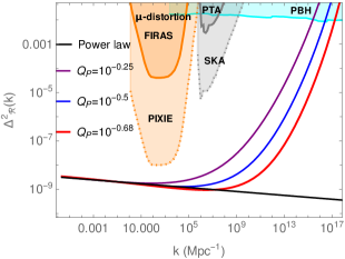
Figure 4: The plots of primordial curvature power spectrum as a function of comoving scale $k$ for the different values of $Q_{G}$ allowed by CMB for Model I ($p=0,q=1$). Fig. 4 and Fig. 4 correspond to $50$ and $60$ efolds of inflation, respectively. The black solid line represents the usually considered power-law primordial power spectrum. The observational constraints from $\mu-$distortion, PTA and SKA are taken from Ref. Chluba:2019kpb . The cyan shaded region represents the excluded region from PBH overproduction.

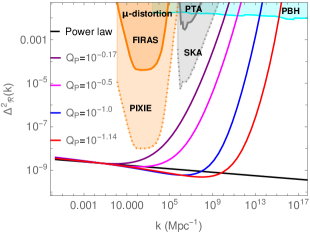
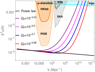
Figure 5: The plots of primordial curvature power spectrum as a function of $k$ for the different values of $Q_{G}$ allowed by CMB for Model II ($p=1,q=1$). Fig. 5 and Fig. 5 correspond to $50$ and $60$ efolds of inflation, respectively. The black solid line represents the usually considered power-law primordial power spectrum. The observational constraints from $\mu-$distortion, PTA and SKA are taken from Ref. Chluba:2019kpb . The cyan shaded region represents the excluded region from PBH overproduction.

We would like to point out that in a canonical setup , the $\lambda\phi^{4}$ warm inflation model with linear dissipation coefficient $\Upsilon\propto T$ does not lead to a sufficient enhancement of the primordial power, while a cubic dissipation $\Upsilon\propto T^{3}$ could lead to PBH generation Arya:2019wck . However, in the non-canonical model, even the linear dissipation coefficient is sufficient to cause enough enhancement in the power spectrum and leads to PBH formation. Also as discussed before, the analytical expression for primordial power spectrum given in Eq. (25) could be studied more carefully, considering the effects of shear viscosity in the radiation fluid. Further, its range of validity has to be examined with the numerical solutions of the coupled stochastic inflaton-radiation system, as done in Refs. (Graham:2009bf ; Bastero-Gil:2021fac ; Ballesteros:2022hjk ). It would be further interesting to construct model similar to Ref. Ballesteros:2022hjk in this setup of warm G-inflation, so as to restrict the inflaton dissipation and the growth of primordial power spectrum. We will address these issues in future works.

VI.2 Initial mass fraction of PBHs

Till now, we have identified the range of comoving scales for our warm inflation models which will be of interest to us. When these modes reenter the horizon during the radiation-dominated era, they collapse into PBHs. We now show the results for the mass and abundance of the generated PBHs from our models, using the formalism discussed in Section V. We plot the initial mass fraction, $\beta^{\prime}(M_{PBH})$ (defined equal to $\gamma^{1/2}\left(\frac{g_{*}}{106.75}\right)^{-1/4}\left(\frac{h}{0.67}\right)^{-2}\beta(M_{PBH})$) versus $M_{PBH}$ for our WI models in Fig. 6 and Fig. 7 corresponding to Model I ($p=0,q=1$) and Model II ($p=0,q=1$), respectively. We infer from these plots that the larger is the $Q_{G}$ value, the more massive are the PBHs. This is because for larger $Q_{G}$, the growth of primordial power is steeper and the large amplitude is attained at a smaller $k$ value. As $M_{PBH}$ is inversely proportional to $k$, this implies a more massive PBH generation. For a review on the observational constraints on $\beta^{\prime}(M_{PBH})$, see Ref. Carr:2020gox .

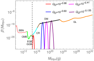
Figure 6: Plots of $\beta^{\prime}(M_{PBH})$ versus $M_{PBH}$ using allowed parameter space of $Q_{G}$ for 6: 50 efolds of inflation, and 6: 60 efolds of inflation in Model I ($p=0,q=1$). The different observational constraints are taken from Ref. Carr:2020gox . Here the acronyms stand for: BBN, CMB, extragalactic $\gamma$-ray background (EGB), galactic $\gamma$-ray background (GGB), cosmic ray (CR), DM, gravitational lensing (GL). The constraints here are for monochromatic mass function of PBHs.

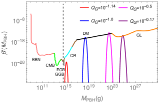
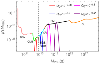
Figure 7: Plots of $\beta^{\prime}(M_{PBH})$ versus $M_{PBH}$ using allowed parameter space of $Q_{G}$ for 7: 50 efolds of inflation, and 7: 60 efolds of inflation in Model II ($p=1,q=1$). The different observational constraints are taken from Ref. Carr:2020gox . The acronyms are the same as in the previous figure.

We can see from Fig. 6 that for 50 efolds of inflation of Model I, PBHs over a mass range $9.3\times 10^{14}$ g $<M_{PBH}<5.6\times 10^{20}$ g can be generated, corresponding to the scales quoted in the previous subsection. Some part of this range lies in the interesting asteroid mass window, thus leading to a possibility of explaining the full dark matter abundance. For $60$ efolds of inflation of Model I, the mass of generated PBHs varies from $9.5\times 10^{10}$ g $<M_{PBH}<4\times 10^{14}$ g, as shown in Fig. 6. These PBHs would have evaporated into Hawking radiation by today and are thus constrained through the PBH evaporation bounds.

Similarly, in Fig. 7, we plot $\beta^{\prime}(M_{PBH})$ versus $M_{PBH}$ using Model II ($p=1,q=1$) for both $50$ and $60$ efolds of inflation. We find that for 50 efolds, shown in Fig. 7, PBHs over a mass range $1.2\times 10^{15}$ g $<M_{PBH}<2\times 10^{25}$ g can be generated, while for $60$ efolds of inflation, mass of the produced PBHs lies between $1\times 10^{14}$ g $<M_{PBH}<9.8\times 10^{19}$ g, as can be seen in Fig. 7. Therefore, we emphasize that in both the scenarios, our model predicts a possibility that PBHs might constitute the total dark matter abundance.

VI.3 PBHs as dark matter

PBHs can contribute significantly or total fraction of the present day DM energy density in certain mass ranges. Here we explore this possibility for our warm inflation models. For this, we calculate and plot the fraction of DM in PBHs, $f_{PBH}$ as a function of PBH mass in Fig. 8 and Fig. 9 using the formalism in Section V. In these plots, we focus on the PBHs mass range greater than $\sim 10^{15}$ g, because the smaller mass PBHs would have evaporated through Hawking radiation and therefore will not contribute much to the DM. The PBHs can explain the full DM when $f_{PBH}=1$. From Fig. (8) we see that in Model I ($p=0,q=1$) with $50$ efolds of inflation, there is a production of the asteroid mass range PBHs which can explain the full DM abundance. We further point out that this model also predicts smaller mass PBHs, with low DM fractional abundance.

Similarly, Fig. 9 indicates that Model II ($p=1,q=1$) with $50$ efolds also generates asteroid mass range PBHs that can constitute the full DM abundance. Along with that, this model also leads to comparably higher and lower mass PBHs, and are constrained through microlensing or evaporation observations, respectively. Further, from Fig. 9, we infer that for $60$ efolds, this model also leads to a possibility of production of PBH DM in the asteroid mass range. This model also predicts smaller mass PBHs which do not contribute significantly to the DM, but are consistent with the evaporation bounds.

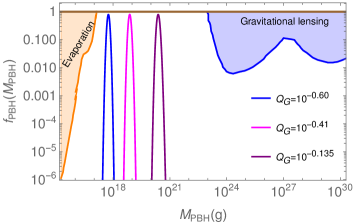
Figure 8: Fraction of DM in PBHs, $f_{PBH}$ vs. $M_{PBH}$ using the allowed parameter space of $Q_{G}$ for 50 efolds of inflation in Model I ($p=0,q=1$). The evaporation and gravitational lensing constraints are taken from Ref. Carr:2020xqk . The maximum fraction in PBHs is bounded from above as $f_{PBH}\leq 1$.

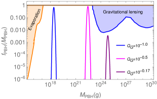
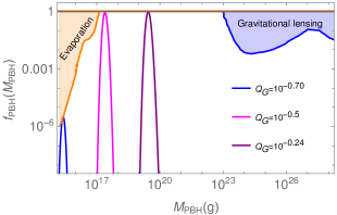
Figure 9: Fraction of dark matter in PBHs, $f_{PBH}$ versus $M_{PBH}$ using the allowed parameter space of $Q_{G}$ for 9: 50 efolds of inflation, and 9: 60 efolds of inflation in Model II ($p=1,q=1$). The evaporation and gravitational lensing constraints are taken from Ref. Carr:2020xqk .

VI.4 Spectrum of scalar induced gravitational waves

The large density fluctuations needed for PBH formation inevitably leads to secondary gravitational wave generation, as discussed before. From Eqs. (46) and (58), we see that the peak GW frequency inversely depends on the PBHs mass. The larger is the mass of PBH, the smaller is the associated peak GW frequency. To explore the spectrum of scalar-induced gravitational waves, we plot $\Omega_{GW}h^{2}$ as a function of frequency in Fig. 10 and Fig. 11 corresponding to the Model I ($p=0,q=1$) and Model II ($p=1,q=1$), respectively. The sensitivity plots for future GW detectors are taken from Ref. Kohri:2018awv .

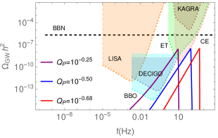
Figure 10: Plot of the gravitational wave energy density, $\Omega_{GW}h^{2}$ induced by the scalar perturbations as a function of frequency for the allowed parameter space of $Q_{G}$ for 10: 50 efolds of inflation, and 10: 60 efolds of inflation, for Model I ($p=0,q=1$). The sensitivity plots for future GW detectors are taken from Ref. Kohri:2018awv . The constraints here are for monochromatic mass function of PBHs.

From Fig. 10, we see that Model I ($p=0,q=1$) with 50 efolds of inflation produces $9.3\times 10^{14}$ g $<M_{PBH}<5.6\times 10^{20}$ g mass PBHs, and generates a GW of peak frequency lying between $\sim(10^{-2}$ $-10$) Hz. These can be detected in the future GW detectors such as LISA, BBO, DECIGO, ET, and CE. Further, the same model with 60 efolds of inflation produces comparably lower PBH mass range, $9.5\times 10^{10}$ g $<M_{PBH}<4\times 10^{14}$ g, and generate comparably higher peak frequency of GW lying between $\sim(10-500$) Hz, as can be seen in Fig. 10. These can be detected in the future GW detector sensitive to high frequency such as ET and CE.

Similarly, Fig. 11 suggests that Model II ($p=1,q=1$) with 50 efolds of inflation produces $1.2\times 10^{15}$ g $<M_{PBH}<2\times 10^{25}$ g mass PBHs and generates GW of peak frequencies lying between $\sim(10^{-4}-10$) Hz. These can be detected in GW observations such as LISA, BBO, DECIGO, and ET. Further, the same model with 60 efolds of inflation produces PBH mass range, $1\times 10^{14}$ g $<M_{PBH}<9.8\times 10^{19}$ g, which generate peak frequency of GW lying between $\sim(0.1-30$) Hz, as shown in Fig. 11. These can also be detected in the future GW detectors such as LISA, BBO, DECIGO, ET, and CE, and thus used to test these models of inflation.

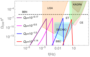
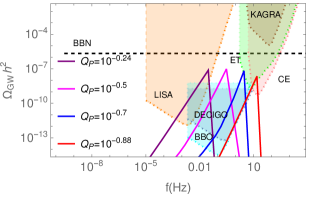
Figure 11: Plot of the gravitational wave energy density, $\Omega_{GW}h^{2}$ induced by the scalar perturbations as a function of frequency for the allowed parameter space of $Q_{G}$ for 11: 50 efolds of inflation, and 11: 60 efolds of inflation, for Model II ($p=1,q=1$). The sensitivity plots for future GW detectors are taken from Ref. Kohri:2018awv .

VII Summary and Discussion

The inflationary paradigm of the early Universe has been extremely successful in explaining various cosmological observations, however, the underlying particle physics model to describe this accelerating phase is not clearly known. The present demand of model building is not only to construct viable models with a physical motivation and interesting phenomenology but also successfully embed them in a UV complete theory. The framework of warm inflation is a general and well-motivated description of inflation wherein the dissipative processes in a coupled inflaton-radiation system drive the evolution of the early Universe. The inflaton dissipates its energy into radiation fields, as a result of which there is a non-zero temperature in the Universe throughout the inflationary phase. The inflaton background evolution as well as its perturbations are modified due to the presence of the thermal bath. Thus, warm inflation leads to unique signatures on the large and small scale observations, and hence important to study.

In this paper, we have studied the scenario of warm Higgs-G inflation, wherein the Standard Model Higgs boson plays the role of the inflaton, and has a Galileon-like non-linear kinetic term, which contributes as an additional frictional term in its evolution. For the quartic Higgs potential and a dissipation coefficient linear in temperature, we have studied two different cases of warm Higgs-G inflation models, with $G(\phi,X)\propto\phi^{2p+1}X^{q}$ and parameter sets ($p=0,q=1$) and ($p=1,q=1$). For a wide range of other parameters, we found that these models are compatible with the CMB Planck observations at large scales. Moreover, contrary to the usual cold inflation, we have shown that these scenarios are consistent with the swampland and the TCC conjectures, implying that they lie in the viable landscape of UV complete theories. In these scenarios, the non-linear kinetic term plays an important role, and we found that when it dominates, the background dynamics of the inflaton and the evolution of small scale perturbations are modified. This leads to a blue-tilted spectrum with an enhanced amplitude at small scales, inducing the generation of PBHs and their associated observational imprints, such as the induced GWs.

In our analysis, we found that PBHs over a wide mass range are generated in these models, in particular, in the asteroid mass range $(10^{17}-10^{23})$ g, which can explain the total dark matter abundance at present. This particular mass range is interesting as it remains unconstrained from observations, and therefore, PBHs produced in any scenario can be the entire dark matter only in this mass range, while in other mass ranges, they can, at most, be a fraction. We have further calculated the secondary scalar induced GWs sourced by these small scale overdense fluctuations in our set-up and found that the induced GW spectrum can be detected in future GW detectors, such as LISA, BBO, DECIGO, ET and CE. In particular, for some GWs spectra, there also exists an interesting possibility of their simultaneous detection with many GW observatories. We conclude that warm inflationary models have interesting prospective signatures, and the forthcoming cosmological probes would be very useful for testing these models.

Furthermore, it is well known that primordial non-Gaussianities strongly affect the abundance of PBHs as they form from the tail of the density distribution. Studies show that in warm inflation, the amplitude and shapes of non-Gaussianities are very different in the strong and weak dissipative regimes. It will therefore be interesting to include and understand the effects of such non-Gaussianities in the warm inflationary models for the calculation of PBH abundance as well as for the induced GW background. We will investigate these interesting aspects in future works.

References

- (1) D. Kazanas, Dynamics of the Universe and Spontaneous Symmetry Breaking, Astrophys. J. 241 (1980) L59–L63.
- (2) K. Sato, First Order Phase Transition of a Vacuum and Expansion of the Universe, Mon. Not. Roy. Astron. Soc. 195 (1981) 467–479.
- (3) A. H. Guth, The Inflationary Universe: A Possible Solution to the Horizon and Flatness Problems, Phys. Rev. D23 (1981) 347–356. [Adv. Ser. Astrophys. Cosmol.3,139(1987)].
- (4) A. D. Linde, A New Inflationary Universe Scenario: A Possible Solution of the Horizon, Flatness, Homogeneity, Isotropy and Primordial Monopole Problems, Phys. Lett. 108B (1982) 389–393. [Adv. Ser. Astrophys. Cosmol.3,149(1987)].
- (5) Planck Collaboration, Y. Akrami et al., Planck 2018 results. X. Constraints on inflation, Astron. Astrophys. 641 (2020) A10, [arXiv:1807.06211].
- (6) D. Baumann, Inflation, in Physics of the large and the small, TASI 09, 1-26 June 2009, pp. 523–686, 2011. arXiv:0907.5424.
- (7) A. D. Linde, Inflationary Cosmology, Lect. Notes Phys. 738 (2008) 1–54, [arXiv:0705.0164].
- (8) A. Riotto, Inflation and the theory of cosmological perturbations, ICTP Lect. Notes Ser. 14 (2003) 317–413, [hep-ph/0210162].
- (9) S. Tsujikawa, Introductory review of cosmic inflation, in 2nd Tah Poe School on Cosmology: Modern Cosmology, 4, 2003. hep-ph/0304257.
- (10) A. D. Linde, Particle physics and inflationary cosmology, vol. 5. 1990.
- (11) J. Rubio, Higgs inflation, Front. Astron. Space Sci. 5 (2019) 50, [arXiv:1807.02376].
- (12) F. L. Bezrukov and M. Shaposhnikov, The Standard Model Higgs boson as the inflaton, Phys. Lett. B 659 (2008) 703–706, [arXiv:0710.3755].
- (13) A. O. Barvinsky, A. Y. Kamenshchik, and A. A. Starobinsky, Inflation scenario via the Standard Model Higgs boson and LHC, JCAP 11 (2008) 021, [arXiv:0809.2104].
- (14) C. Germani and A. Kehagias, New Model of Inflation with Non-minimal Derivative Coupling of Standard Model Higgs Boson to Gravity, Phys. Rev. Lett. 105 (2010) 011302, [arXiv:1003.2635].
- (15) C. Armendariz-Picon, T. Damour, and V. F. Mukhanov, k - inflation, Phys. Lett. B 458 (1999) 209–218, [hep-th/9904075].
- (16) N. Arkani-Hamed, P. Creminelli, S. Mukohyama, and M. Zaldarriaga, Ghost inflation, JCAP 04 (2004) 001, [hep-th/0312100].
- (17) M. Alishahiha, E. Silverstein, and D. Tong, DBI in the sky, Phys. Rev. D 70 (2004) 123505, [hep-th/0404084].
- (18) C. Deffayet, G. Esposito-Farese, and A. Vikman, Covariant Galileon, Phys. Rev. D 79 (2009) 084003, [arXiv:0901.1314].
- (19) C. Deffayet, S. Deser, and G. Esposito-Farese, Generalized Galileons: All scalar models whose curved background extensions maintain second-order field equations and stress-tensors, Phys. Rev. D 80 (2009) 064015, [arXiv:0906.1967].
- (20) T. Kobayashi, M. Yamaguchi, and J. Yokoyama, Generalized G-inflation: Inflation with the most general second-order field equations, Prog. Theor. Phys. 126 (2011) 511–529, [arXiv:1105.5723].
- (21) N. Chow and J. Khoury, Galileon Cosmology, Phys. Rev. D 80 (2009) 024037, [arXiv:0905.1325].
- (22) F. P. Silva and K. Koyama, Self-Accelerating Universe in Galileon Cosmology, Phys. Rev. D 80 (2009) 121301, [arXiv:0909.4538].
- (23) T. Kobayashi, H. Tashiro, and D. Suzuki, Evolution of linear cosmological perturbations and its observational implications in Galileon-type modified gravity, Phys. Rev. D 81 (2010) 063513, [arXiv:0912.4641].
- (24) T. Kobayashi, Cosmic expansion and growth histories in Galileon scalar-tensor models of dark energy, Phys. Rev. D 81 (2010) 103533, [arXiv:1003.3281].
- (25) R. Gannouji and M. Sami, Galileon gravity and its relevance to late time cosmic acceleration, Phys. Rev. D 82 (2010) 024011, [arXiv:1004.2808].
- (26) A. De Felice, S. Mukohyama, and S. Tsujikawa, Density perturbations in general modified gravitational theories, Phys. Rev. D 82 (2010) 023524, [arXiv:1006.0281].
- (27) A. De Felice and S. Tsujikawa, Cosmology of a covariant Galileon field, Phys. Rev. Lett. 105 (2010) 111301, [arXiv:1007.2700].
- (28) T. Kobayashi, M. Yamaguchi, and J. Yokoyama, G-inflation: Inflation driven by the Galileon field, Phys. Rev. Lett. 105 (2010) 231302, [arXiv:1008.0603].
- (29) S. Mizuno and K. Koyama, Primordial non-Gaussianity from the DBI Galileons, Phys. Rev. D 82 (2010) 103518, [arXiv:1009.0677].
- (30) C. Burrage, C. de Rham, D. Seery, and A. J. Tolley, Galileon inflation, JCAP 01 (2011) 014, [arXiv:1009.2497].
- (31) P. Creminelli, G. D’Amico, M. Musso, J. Norena, and E. Trincherini, Galilean symmetry in the effective theory of inflation: new shapes of non-Gaussianity, JCAP 02 (2011) 006, [arXiv:1011.3004].
- (32) J. Ohashi and S. Tsujikawa, Potential-driven Galileon inflation, JCAP 10 (2012) 035, [arXiv:1207.4879].
- (33) K. Kamada, T. Kobayashi, M. Yamaguchi, and J. Yokoyama, Higgs G-inflation, Phys. Rev. D 83 (2011) 083515, [arXiv:1012.4238].
- (34) K. Kamada, T. Kobayashi, T. Kunimitsu, M. Yamaguchi, and J. Yokoyama, Graceful exit from Higgs inflation, Phys. Rev. D 88 (2013), no. 12 123518, [arXiv:1309.7410].
- (35) M. Motaharfar, E. Massaeli, and H. R. Sepangi, Power spectra in warm G-inflation and its consistency: stochastic approach, Phys. Rev. D 96 (2017), no. 10 103541, [arXiv:1705.04049].
- (36) R. Herrera, G-Warm inflation, JCAP 05 (2017) 029, [arXiv:1701.07934].
- (37) M. Motaharfar, E. Massaeli, and H. R. Sepangi, Warm Higgs G-inflation: predictions and constraints from Planck 2015 likelihood, JCAP 10 (2018) 002, [arXiv:1807.09548].
- (38) A. Berera and L.-Z. Fang, Thermally induced density perturbations in the inflation era, Phys. Rev. Lett. 74 (1995) 1912–1915, [astro-ph/9501024].
- (39) A. Berera, Warm inflation, Phys. Rev. Lett. 75 (1995) 3218–3221, [astro-ph/9509049].
- (40) A. Berera, M. Gleiser, and R. O. Ramos, A First principles warm inflation model that solves the cosmological horizon / flatness problems, Phys. Rev. Lett. 83 (1999) 264–267, [hep-ph/9809583].
- (41) A. Berera, The warm inflationary universe, Contemp. Phys. 47 (2006) 33–49, [arXiv:0809.4198].
- (42) A. Berera, I. G. Moss, and R. O. Ramos, Warm Inflation and its Microphysical Basis, Rept. Prog. Phys. 72 (2009) 026901, [arXiv:0808.1855].
- (43) O. Grn, Warm Inflation, Universe 2 (2016), no. 3 20.
- (44) L. Visinelli, Observational Constraints on Monomial Warm Inflation, JCAP 1607 (2016), no. 07 054, [arXiv:1605.06449].
- (45) M. Benetti and R. O. Ramos, Warm inflation dissipative effects: predictions and constraints from the Planck data, Phys. Rev. D95 (2017), no. 2 023517, [arXiv:1610.08758].
- (46) R. Arya, A. Dasgupta, G. Goswami, J. Prasad, and R. Rangarajan, Revisiting CMB constraints on warm inflation, JCAP 1802 (2018), no. 02 043, [arXiv:1710.11109].
- (47) R. Arya and R. Rangarajan, Study of warm inflationary models and their parameter estimation from CMB, Int. J. Mod. Phys. D 29 (2020), no. 08 2050055, [arXiv:1812.03107].
- (48) M. Bastero-Gil, S. Bhattacharya, K. Dutta, and M. R. Gangopadhyay, Constraining Warm Inflation with CMB data, JCAP 02 (2018) 054, [arXiv:1710.10008].
- (49) S. Gupta, A. Berera, A. F. Heavens, and S. Matarrese, Non-Gaussian signatures in the cosmic background radiation from warm inflation, Phys. Rev. D66 (2002) 043510, [astro-ph/0205152].
- (50) I. G. Moss and T. Yeomans, Non-gaussianity in the strong regime of warm inflation, JCAP 1108 (2011) 009, [arXiv:1102.2833].
- (51) M. Bastero-Gil, A. Berera, I. G. Moss, and R. O. Ramos, Theory of non-Gaussianity in warm inflation, JCAP 12 (2014) 008, [arXiv:1408.4391].
- (52) M. Mirbabayi and A. Gruzinov, Shapes of non-Gaussianity in warm inflation, JCAP 02 (2023) 012, [arXiv:2205.13227].
- (53) A. Berera, Warm inflation solution to the eta problem, hep-ph/0401139. [PoSAHEP2003,069(2003)].
- (54) J. a. G. Rosa and L. B. Ventura, Warm Little Inflaton becomes Cold Dark Matter, Phys. Rev. Lett. 122 (2019), no. 16 161301, [arXiv:1811.05493].
- (55) J. a. G. Rosa and L. B. Ventura, Warm Little Inflaton becomes Dark Energy, Phys. Lett. B 798 (2019) 134984, [arXiv:1906.11835].
- (56) P. M. Sá, Triple unification of inflation, dark energy, and dark matter in two-scalar-field cosmology, Phys. Rev. D 102 (2020), no. 10 103519, [arXiv:2007.07109].
- (57) R. D’Agostino and O. Luongo, Cosmological viability of a double field unified model from warm inflation, Phys. Lett. B 829 (2022) 137070, [arXiv:2112.12816].
- (58) M. Bastero-Gil, A. Berera, R. O. Ramos, and J. G. Rosa, Warm baryogenesis, Phys. Lett. B 712 (2012) 425–429, [arXiv:1110.3971].
- (59) S. Basak, S. Bhattacharya, M. R. Gangopadhyay, N. Jaman, R. Rangarajan, and M. Sami, The paradigm of warm quintessential inflation and spontaneous baryogenesis, JCAP 03 (2022), no. 03 063, [arXiv:2110.00607].
- (60) S. Das, Warm Inflation in the light of Swampland Criteria, Phys. Rev. D99 (2019), no. 6 063514, [arXiv:1810.05038].
- (61) M. Motaharfar, V. Kamali, and R. O. Ramos, Warm inflation as a way out of the swampland, Phys. Rev. D99 (2019), no. 6 063513, [arXiv:1810.02816].
- (62) Y. B. Zel’dovich and I. D. Novikov, The Hypothesis of Cores Retarded During Expansion and the Hot Cosmological Model, Soviet Astronomy 10 (1967) 602.
- (63) S. Hawking, Gravitationally collapsed objects of very low mass, Mon. Not. Roy. Astron. Soc. 152 (1971) 75.
- (64) B. J. Carr and S. W. Hawking, Black holes in the early Universe, Mon. Not. Roy. Astron. Soc. 168 (1974) 399–415.
- (65) B. J. Carr, The Primordial black hole mass spectrum, Astrophys. J. 201 (1975) 1–19.
- (66) S. W. Hawking, I. G. Moss, and J. M. Stewart, Bubble Collisions in the Very Early Universe, Phys. Rev. D26 (1982) 2681.
- (67) C. J. Hogan, Massive Black Holes generated by Cosmic Strings, Phys. Lett. 143B (1984) 87–91.
- (68) R. R. Caldwell, A. Chamblin, and G. W. Gibbons, Pair creation of black holes by domain walls, Phys. Rev. D53 (1996) 7103–7114, [hep-th/9602126].
- (69) J. Garcia-Bellido, A. D. Linde, and D. Wands, Density perturbations and black hole formation in hybrid inflation, Phys. Rev. D54 (1996) 6040–6058, [astro-ph/9605094].
- (70) E. Bugaev and P. Klimai, Formation of primordial black holes from non-Gaussian perturbations produced in a waterfall transition, Phys. Rev. D 85 (2012) 103504, [arXiv:1112.5601].
- (71) S. Clesse and J. García-Bellido, Massive Primordial Black Holes from Hybrid Inflation as Dark Matter and the seeds of Galaxies, Phys. Rev. D 92 (2015), no. 2 023524, [arXiv:1501.07565].
- (72) S. M. Leach, I. J. Grivell, and A. R. Liddle, Black hole constraints on the running mass inflation model, Phys. Rev. D62 (2000) 043516, [astro-ph/0004296].
- (73) K. Kohri, D. H. Lyth, and A. Melchiorri, Black hole formation and slow-roll inflation, JCAP 04 (2008) 038, [arXiv:0711.5006].
- (74) M. Drees and E. Erfani, Running-Mass Inflation Model and Primordial Black Holes, JCAP 1104 (2011) 005, [arXiv:1102.2340].
- (75) H. Motohashi and W. Hu, Primordial Black Holes and Slow-Roll Violation, Phys. Rev. D96 (2017), no. 6 063503, [arXiv:1706.06784].
- (76) L. Alabidi and K. Kohri, Generating Primordial Black Holes Via Hilltop-Type Inflation Models, Phys. Rev. D 80 (2009) 063511, [arXiv:0906.1398].
- (77) K. Kohri, C.-M. Lin, and T. Matsuda, Primordial black holes from the inflating curvaton, Phys. Rev. D87 (2013), no. 10 103527, [arXiv:1211.2371].
- (78) M. Kawasaki, N. Kitajima, and T. T. Yanagida, Primordial black hole formation from an axionlike curvaton model, Phys. Rev. D 87 (2013), no. 6 063519, [arXiv:1207.2550].
- (79) K. Ando, K. Inomata, M. Kawasaki, K. Mukaida, and T. T. Yanagida, Primordial black holes for the LIGO events in the axionlike curvaton model, Phys. Rev. D 97 (2018), no. 12 123512, [arXiv:1711.08956].
- (80) M. Kawasaki, N. Sugiyama, and T. Yanagida, Primordial black hole formation in a double inflation model in supergravity, Phys. Rev. D 57 (1998) 6050–6056, [hep-ph/9710259].
- (81) K. Dimopoulos, T. Markkanen, A. Racioppi, and V. Vaskonen, Primordial Black Holes from Thermal Inflation, JCAP 1907 (2019) 046, [arXiv:1903.09598].
- (82) T. Bringmann, C. Kiefer, and D. Polarski, Primordial black holes from inflationary models with and without broken scale invariance, Phys. Rev. D65 (2002) 024008, [astro-ph/0109404].
- (83) J. Garcia-Bellido and E. Ruiz Morales, Primordial black holes from single field models of inflation, Phys. Dark Univ. 18 (2017) 47–54, [arXiv:1702.03901].
- (84) G. Ballesteros and M. Taoso, Primordial black hole dark matter from single field inflation, Phys. Rev. D97 (2018), no. 2 023501, [arXiv:1709.05565].
- (85) C. Germani and T. Prokopec, On primordial black holes from an inflection point, Phys. Dark Univ. 18 (2017) 6–10, [arXiv:1706.04226].
- (86) N. Bhaumik and R. K. Jain, Primordial black holes dark matter from inflection point models of inflation and the effects of reheating, JCAP 01 (2020) 037, [arXiv:1907.04125].
- (87) S. S. Mishra and V. Sahni, Primordial Black Holes from a tiny bump/dip in the Inflaton potential, JCAP 04 (2020) 007, [arXiv:1911.00057].
- (88) M. Drees and E. Erfani, Running Spectral Index and Formation of Primordial Black Hole in Single Field Inflation Models, JCAP 1201 (2012) 035, [arXiv:1110.6052].
- (89) K. Kohri and T. Terada, Primordial Black Hole Dark Matter and LIGO/Virgo Merger Rate from Inflation with Running Spectral Indices: Formation in the Matter- and/or Radiation-Dominated Universe, Class. Quant. Grav. 35 (2018), no. 23 235017, [arXiv:1802.06785].
- (90) D. Ghosh and A. K. Mishra, Gravitation Wave signal from Asteroid mass Primordial Black Hole Dark Matter, arXiv:2208.14279.
- (91) O. Özsoy, S. Parameswaran, G. Tasinato, and I. Zavala, Mechanisms for Primordial Black Hole Production in String Theory, JCAP 07 (2018) 005, [arXiv:1803.07626].
- (92) R. Zhai, H. Yu, and P. Wu, Growth of power spectrum due to decrease of sound speed during inflation, Phys. Rev. D 106 (2022), no. 2 023517, [arXiv:2207.12745].
- (93) Y.-F. Cai, X. Tong, D.-G. Wang, and S.-F. Yan, Primordial Black Holes from Sound Speed Resonance during Inflation, Phys. Rev. Lett. 121 (2018), no. 8 081306, [arXiv:1805.03639].
- (94) Z. Zhou, J. Jiang, Y.-F. Cai, M. Sasaki, and S. Pi, Primordial black holes and gravitational waves from resonant amplification during inflation, Phys. Rev. D 102 (2020), no. 10 103527, [arXiv:2010.03537].
- (95) A. M. Green and A. R. Liddle, Constraints on the density perturbation spectrum from primordial black holes, Phys. Rev. D56 (1997) 6166–6174, [astro-ph/9704251].
- (96) A. S. Josan, A. M. Green, and K. A. Malik, Generalised constraints on the curvature perturbation from primordial black holes, Phys. Rev. D79 (2009) 103520, [arXiv:0903.3184].
- (97) B. J. Carr, K. Kohri, Y. Sendouda, and J. Yokoyama, New cosmological constraints on primordial black holes, Phys. Rev. D81 (2010) 104019, [arXiv:0912.5297].
- (98) G. Sato-Polito, E. D. Kovetz, and M. Kamionkowski, Constraints on the primordial curvature power spectrum from primordial black holes, Phys. Rev. D100 (2019), no. 6 063521, [arXiv:1904.10971].
- (99) N. Bhaumik, A. Ghoshal, R. K. Jain, and M. Lewicki, Distinct signatures of spinning PBH domination and evaporation: doubly peaked gravitational waves, dark relics and CMB complementarity, arXiv:2212.00775.
- (100) N. Bhaumik and R. K. Jain, Small scale induced gravitational waves from primordial black holes, a stringent lower mass bound, and the imprints of an early matter to radiation transition, Phys. Rev. D 104 (2021), no. 2 023531, [arXiv:2009.10424].
- (101) N. Bhaumik, A. Ghoshal, and M. Lewicki, Doubly peaked induced stochastic gravitational wave background: testing baryogenesis from primordial black holes, JHEP 07 (2022) 130, [arXiv:2205.06260].
- (102) M. Sasaki, T. Suyama, T. Tanaka, and S. Yokoyama, Primordial black holes - perspectives in gravitational wave astronomy, Class. Quant. Grav. 35 (2018), no. 6 063001, [arXiv:1801.05235].
- (103) B. Carr, K. Kohri, Y. Sendouda, and J. Yokoyama, Constraints on primordial black holes, Rept. Prog. Phys. 84 (2021), no. 11 116902, [arXiv:2002.12778].
- (104) B. Carr and F. Kuhnel, Primordial Black Holes as Dark Matter: Recent Developments, Ann. Rev. Nucl. Part. Sci. 70 (2020) 355–394, [arXiv:2006.02838].
- (105) A. M. Green and B. J. Kavanagh, Primordial Black Holes as a dark matter candidate, J. Phys. G 48 (2021), no. 4 043001, [arXiv:2007.10722].
- (106) S. Mollerach, D. Harari, and S. Matarrese, CMB polarization from secondary vector and tensor modes, Phys. Rev. D 69 (2004) 063002, [astro-ph/0310711].
- (107) K. N. Ananda, C. Clarkson, and D. Wands, The Cosmological gravitational wave background from primordial density perturbations, Phys. Rev. D 75 (2007) 123518, [gr-qc/0612013].
- (108) D. Baumann, P. J. Steinhardt, K. Takahashi, and K. Ichiki, Gravitational Wave Spectrum Induced by Primordial Scalar Perturbations, Phys. Rev. D 76 (2007) 084019, [hep-th/0703290].
- (109) K. Kohri and T. Terada, Semianalytic calculation of gravitational wave spectrum nonlinearly induced from primordial curvature perturbations, Phys. Rev. D 97 (2018), no. 12 123532, [arXiv:1804.08577].
- (110) R. Arya, Formation of Primordial Black Holes from Warm Inflation, JCAP 09 (2020) 042, [arXiv:1910.05238].
- (111) R. Arya and A. K. Mishra, Scalar induced gravitational waves from warm inflation, Phys. Dark Univ. 37 (2022) 101116, [arXiv:2204.02896].
- (112) M. Bastero-Gil and M. S. Díaz-Blanco, Gravity waves and primordial black holes in scalar warm little inflation, JCAP 12 (2021), no. 12 052, [arXiv:2105.08045].
- (113) M. Correa, M. R. Gangopadhyay, N. Jaman, and G. J. Mathews, Primordial black-hole dark matter via warm natural inflation, Phys. Lett. B 835 (2022) 137510, [arXiv:2207.10394].
- (114) G. Ballesteros, M. A. G. García, A. P. Rodríguez, M. Pierre, and J. Rey, Primordial black holes and gravitational waves from dissipation during inflation, JCAP 12 (2022) 006, [arXiv:2208.14978].
- (115) J. Lin, Q. Gao, Y. Gong, Y. Lu, C. Zhang, and F. Zhang, Primordial black holes and secondary gravitational waves from and inflation, Phys. Rev. D 101 (2020), no. 10 103515, [arXiv:2001.05909].
- (116) J. Lin, S. Gao, Y. Gong, Y. Lu, Z. Wang, and F. Zhang, Primordial black holes and scalar induced gravitational waves from Higgs inflation with non-canonical kinetic term, arXiv:2111.01362.
- (117) Q. Gao, Y. Gong, and Z. Yi, Primordial black holes and secondary gravitational waves from natural inflation, Nucl. Phys. B 969 (2021) 115480, [arXiv:2012.03856].
- (118) Z. Yi, Q. Gao, Y. Gong, and Z.-h. Zhu, Primordial black holes and scalar-induced secondary gravitational waves from inflationary models with a noncanonical kinetic term, Phys. Rev. D 103 (2021), no. 6 063534, [arXiv:2011.10606].
- (119) Z. Teimoori, K. Rezazadeh, M. A. Rasheed, and K. Karami, Mechanism of primordial black holes production and secondary gravitational waves in -attractor Galileon inflationary scenario, arXiv:2107.07620.
- (120) M. Gleiser and R. O. Ramos, Microphysical approach to nonequilibrium dynamics of quantum fields, Phys. Rev. D50 (1994) 2441–2455, [hep-ph/9311278].
- (121) A. Berera, M. Gleiser, and R. O. Ramos, Strong dissipative behavior in quantum field theory, Phys. Rev. D 58 (1998) 123508, [hep-ph/9803394].
- (122) A. Berera, I. G. Moss, and R. O. Ramos, Local Approximations for Effective Scalar Field Equations of Motion, Phys. Rev. D 76 (2007) 083520, [arXiv:0706.2793].
- (123) L. M. H. Hall, I. G. Moss, and A. Berera, Scalar perturbation spectra from warm inflation, Phys. Rev. D69 (2004) 083525, [astro-ph/0305015].
- (124) I. G. Moss and C. Xiong, On the consistency of warm inflation, JCAP 0811 (2008) 023, [arXiv:0808.0261].
- (125) I. G. Moss and C. Xiong, Dissipation coefficients for supersymmetric inflatonary models, hep-ph/0603266.
- (126) M. Bastero-Gil, A. Berera, and R. O. Ramos, Dissipation coefficients from scalar and fermion quantum field interactions, JCAP 1109 (2011) 033, [arXiv:1008.1929].
- (127) M. Bastero-Gil, A. Berera, R. O. Ramos, and J. G. Rosa, General dissipation coefficient in low-temperature warm inflation, JCAP 1301 (2013) 016, [arXiv:1207.0445].
- (128) M. Bastero-Gil, A. Berera, R. Hernández-Jiménez, and J. G. Rosa, Warm inflation within a supersymmetric distributed mass model, Phys. Rev. D99 (2019), no. 10 103520, [arXiv:1812.07296].
- (129) M. Bastero-Gil, A. Berera, R. O. Ramos, and J. a. G. Rosa, Towards a reliable effective field theory of inflation, Phys. Lett. B 813 (2021) 136055, [arXiv:1907.13410].
- (130) M. Bastero-Gil, A. Berera, R. O. Ramos, and J. G. Rosa, Warm Little Inflaton, Phys. Rev. Lett. 117 (2016), no. 15 151301, [arXiv:1604.08838].
- (131) C. Graham and I. G. Moss, Density fluctuations from warm inflation, JCAP 0907 (2009) 013, [arXiv:0905.3500].
- (132) R. O. Ramos and L. A. da Silva, Power spectrum for inflation models with quantum and thermal noises, JCAP 1303 (2013) 032, [arXiv:1302.3544].
- (133) M. Bastero-Gil, A. Berera, and R. O. Ramos, Shear viscous effects on the primordial power spectrum from warm inflation, JCAP 07 (2011) 030, [arXiv:1106.0701].
- (134) C. Deffayet, O. Pujolas, I. Sawicki, and A. Vikman, Imperfect Dark Energy from Kinetic Gravity Braiding, JCAP 10 (2010) 026, [arXiv:1008.0048].
- (135) G. Obied, H. Ooguri, L. Spodyneiko, and C. Vafa, De Sitter Space and the Swampland, arXiv:1806.08362.
- (136) A. Kehagias and A. Riotto, A note on Inflation and the Swampland, Fortsch. Phys. 66 (2018), no. 10 1800052, [arXiv:1807.05445].
- (137) W. H. Kinney, S. Vagnozzi, and L. Visinelli, The zoo plot meets the swampland: mutual (in)consistency of single-field inflation, string conjectures, and cosmological data, Class. Quant. Grav. 36 (2019), no. 11 117001, [arXiv:1808.06424].
- (138) A. Bedroya and C. Vafa, Trans-Planckian Censorship and the Swampland, JHEP 09 (2020) 123, [arXiv:1909.11063].
- (139) A. Bedroya, R. Brandenberger, M. Loverde, and C. Vafa, Trans-Planckian Censorship and Inflationary Cosmology, Phys. Rev. D 101 (2020), no. 10 103502, [arXiv:1909.11106].
- (140) A. Achúcarro and G. A. Palma, The string swampland constraints require multi-field inflation, JCAP 02 (2019) 041, [arXiv:1807.04390].
- (141) A. Ashoorioon, Rescuing Single Field Inflation from the Swampland, Phys. Lett. B 790 (2019) 568–573, [arXiv:1810.04001].
- (142) S. Das, Note on single-field inflation and the swampland criteria, Phys. Rev. D 99 (2019), no. 8 083510, [arXiv:1809.03962].
- (143) V. Kamali, M. Motaharfar, and R. O. Ramos, Warm brane inflation with an exponential potential: a consistent realization away from the swampland, Phys. Rev. D 101 (2020), no. 2 023535, [arXiv:1910.06796].
- (144) S. Das, G. Goswami, and C. Krishnan, Swampland, axions, and minimal warm inflation, Phys. Rev. D 101 (2020), no. 10 103529, [arXiv:1911.00323].
- (145) S. Das and R. O. Ramos, Runaway potentials in warm inflation satisfying the swampland conjectures, Phys. Rev. D 102 (2020), no. 10 103522, [arXiv:2007.15268].
- (146) O. Bertolami and P. M. Sá, Multi-field cold and warm inflation and the de Sitter swampland conjectures, JCAP 09 (2022) 001, [arXiv:2204.13794].
- (147) F. B. M. d. Santos, R. Silva, S. S. da Costa, M. Benetti, and J. S. Alcaniz, Warm -exponential inflation and the Swampland Conjectures, arXiv:2209.06153.
- (148) W. H. Press and P. Schechter, Formation of galaxies and clusters of galaxies by selfsimilar gravitational condensation, Astrophys. J. 187 (1974) 425–438.
- (149) P. Montero-Camacho, X. Fang, G. Vasquez, M. Silva, and C. M. Hirata, Revisiting constraints on asteroid-mass primordial black holes as dark matter candidates, JCAP 08 (2019) 031, [arXiv:1906.05950].
- (150) J. Chluba et al., Spectral Distortions of the CMB as a Probe of Inflation, Recombination, Structure Formation and Particle Physics: Astro2020 Science White Paper, Bull. Am. Astron. Soc. 51 (2019), no. 3 184, [arXiv:1903.04218].