Universality laws for Gaussian mixtures in generalized linear models

Abstract

Let $({\bm{x}}_{i},y_{i})_{i=1,\dots,n}$ denote independent samples from a general mixture distribution $\sum_{c\in\mathcal{C}}\rho_{c}P_{c}^{{\bm{x}}}$, and consider the hypothesis class of generalized linear models $\hat{y}=F({\bm{\Theta}}^{\top}{\bm{x}})$. In this work, we investigate the asymptotic joint statistics of the family of generalized linear estimators $({\bm{\Theta}}_{1},\dots,{\bm{\Theta}}_{M})$ obtained either from (a) minimizing an empirical risk $\hat{R}_{n}({\bm{\Theta}};{\bm{X}},{\bm{y}})$ or (b) sampling from the associated Gibbs measure $\exp(-\beta n\hat{R}_{n}({\bm{\Theta}};{\bm{X}},{\bm{y}}))$. Our main contribution is to characterize under which conditions the asymptotic joint statistics of this family depends (on a weak sense) only on the means and covariances of the class conditional features distribution $P_{c}^{{\bm{x}}}$. In particular, this allow us to prove the universality of different quantities of interest, such as the training and generalization errors, redeeming a recent line of work in high-dimensional statistics working under the Gaussian mixture hypothesis. Finally, we discuss the applications of our results to different machine learning tasks of interest, such as ensembling and uncertainty quantification.

1 Introduction

A recurrent topic in high-dimensional statistics is the investigation of the typical properties of signal processing and machine learning methods on synthetic, i.i.d. Gaussian data, a scenario often known under the umbrella of Gaussian design (donoho2009observed; 5730603; Monajemi2013; candes2020phase; Bartlett30063). A less restrictive assumption arises when considering that many machine learning tasks deal with data partitioned into a fixed number of classes. In these cases, the data distribution is naturally described by a mixture model, where each sample is generated conditionally on the class. In other words: data is generated by first sampling the class assignment and then generating the input conditioned on the class. Arguably the simplest example of such distributions is that of a Gaussian mixture, which shall be our focus in this work.

Gaussian mixtures are a popular model in high-dimensional statistics since, besides being an universal approximator, they often lead to mathematically tractable problems. Indeed, a recent line of work has analyzed the asymptotic performance of a large class of machine learning problems in the proportional high-dimensional limit under the Gaussian mixture data assumption, see e.g. mai2019high; mignacco2020role; taheri2020optimality; kini2021phase; wang2021benign; refinetti2021classifying; loureiro2021learning_gm. The key goal of the present work is to show that this assumption, and hence the conclusions derived therein, are far more general than previously anticipated.

We build on a recent line of works (goldt2020gaussian; hu2020universality; montanari2022universality) that have proven the asymptotic (single) Gaussian equivalence of generalized linear estimation on non-linear feature maps satisfying certain regularities conditions, a topic that has started with the work of el2010spectrum on kernel matrices. Furthermore, there is strong empirical evidence that Gaussian universality holds in a more general sense (loureiro2021learning). A crucial limitation of the results in hu2020universality; montanari2022universality, however, is the assumption of a target function depending on linear projections in the latent or feature space. Instead, we consider a rich class of mixture distributions, allowing arbitrary dependence between the class labels and the data.

Here, we extend this line of works and provide rigorous justification for universality in various settings such as empirical risk minimization (ERM), sampling, ensembling, etc. for general mixture distributions. Namely, we shall show that the statistics of generalized estimators obtained either from ERM or sampling on a mixture model asymptotically agrees (in a weak sense) with the statistics of estimators from the same class trained on a Gaussian mixture model with matching first and second order moments. In particular, this implies the universality of different quantities of interest, such as the training and generalization errors.

Our main contributions are as follows:

• We extend the Gaussian universality of empirical risk minimization theorems in goldt2020gaussian; hu2020universality; montanari2022universality to generic mixture distribution and an equivalent mixture of Gaussians. In particular, we show that a Gaussian mixture observed through a random feature map is also a Gaussian mixture in the high-dimensional limit, a fact used for instance (without rigorous justification) in refinetti2021classifying; loureiro2021learning_gm.

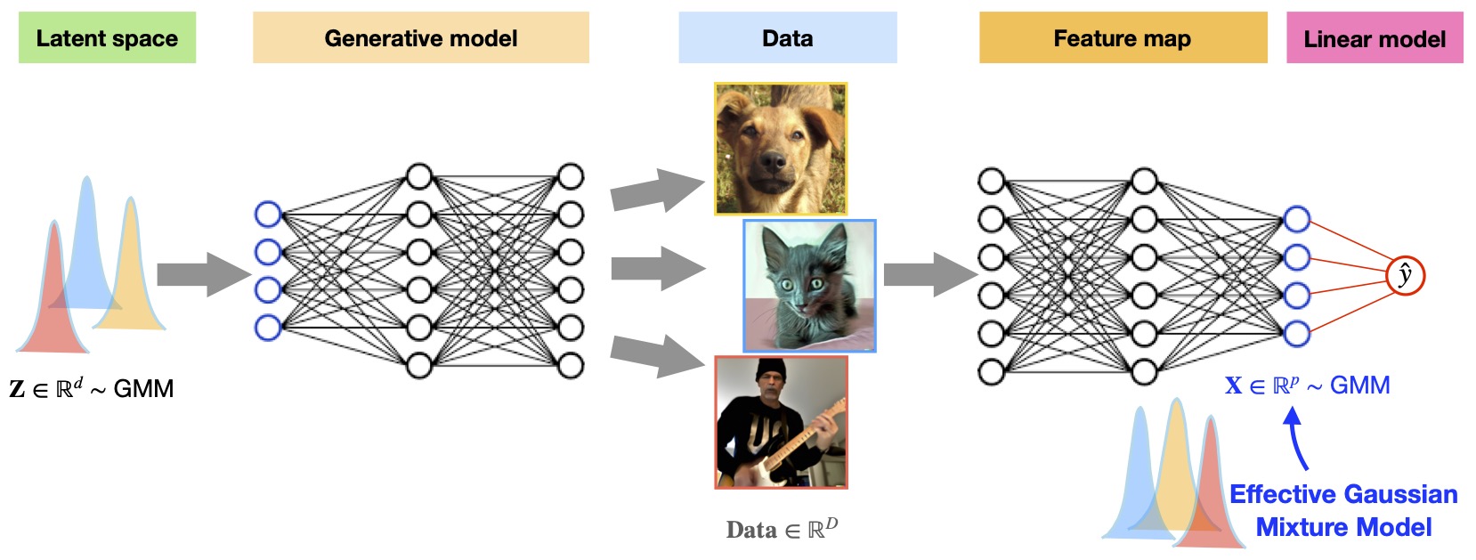
Figure 1: Illustration of Corollary LABEL:thm:main_gaussian_universality: high-dimensional data generated by generative neural networks starting from a mixture of Gaussian in latent space (${\bf z}\in{\mathbb{R}}^{H}$) are (with conditions on the weights matrices) equivalent, in high-dimension and for generalized linear models, to data sampled from a Gaussian mixture. A concrete example is shown in Fig. 2.

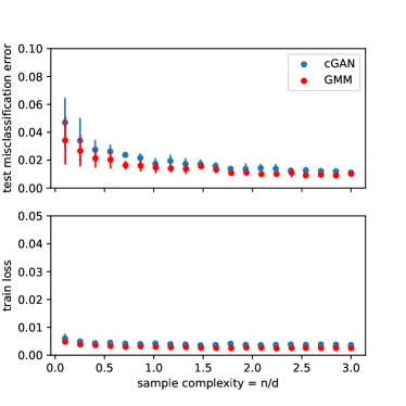
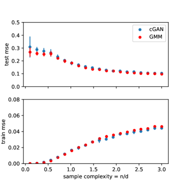
Figure 2: Illustration of the universality scenario described in Fig.1. Logistic (left) & ridge (right) regression test (up) and training (bottom) errors are shown versus the sample complexity $\alpha=\nicefrac{{n}}{{d}}$ for an odd vs. even binary classification task on two data models: Blue dots data generated from a conditional GAN (Mirza2014) trained on the fashion-MNIST dataset (xiao2017) and pre-processed with a random features map $\bm{x}\mapsto\tanh(\mathrm{W}\bm{x})$ with Gaussian weights $W\!\in\!\mathbb{R}^{1176\times 784}$; Red dots are the $10$- clusters Gaussian mixture model with means and covariances matching each fashion-MNIST cluster conditioned on labels ($\ell_{2}$ regularization is $\lambda\!=\!10^{-4}$). Details on the simulations are discussed in Appendix LABEL:sec:app:numerics.

• A consequence of our results is that, with conditions on the matrix weights, data generated by conditional Generative Adversarial Networks (cGAN) behave as a Gaussian mixture when observed through the prism of generalized linear models (kernels, feature maps, etc…), as illustrated in Figs 1 and 2. This further generalizes the work of seddik_2020_random that only considered the universality of Gram matrices for GAN generated data through the prism of random matrix theory.

• We consider setups involving multiple sets of parameters arising from simultaneous minimization of different objectives as well as sampling from Gibbs distributions defined by the empirical risk. This provides a unified framework for establishing the asymptotic universality of arbitrary functions of the set of minimizers or samples from different Gibbs distributions. For instance, it includes ensembling (loureiro2022fluc)) and uncertainty quantification (Clarte2022a; Clarte2022b) settings.

• We finally show how, in common setups, universality holds for a large class of functions, leading to the equivalence between the distributions of the minimizers themselves, and provide a theorem for their weak convergence.

Related work —

Universality is an important topic in applied mathematics, as it motivates the scope of tractable mathematical models. It has been extensively studied in the context of random matrix theory (Tao2011; Tao2012), signal processing problems (donoho2009observed; 5730603; Monajemi2013; NIPS2017_136f9513; 8006947; NEURIPS2019_dffbb6ef; Abbara_2020; Dudeja2022) and kernel methods (el2010spectrum; Lu2022; Misiakiewicz2022). Closer to us is the recent stream of works that investigated the Gaussian universality of the asymptotic error of generalized linear models trained on non-linear features, starting from single-layer random feature maps (montanari2019generalization; gerace2020generalisation; hu2020universality; dhifallah2021) and later extended to single-layer NTK (montanari2022universality) and deep random features (Schroder2023). These results, together with numerical observations that Gaussian universality holds for more general classes of features, led to the formulation of different Gaussian equivalence conjectures (goldt2019modelling; goldt2020gaussian; loureiro2021learning). A complementary line of research has investigated cases in which the distribution of the features is multi-modal, suggesting a Gaussian mixture universality class instead (louart2018random; seddik_2020_random; seddik_2021_unexpected). A bridge between these two lines of work has been recently investigated for generalized linear estimation with random labels in gerace2022.

2 Setting and motivation

Consider a supervised learning problem where the training data $(\bm{x}_{i},y_{i})\in\mathbb{R}^{p}\times\mathcal{Y}$, $i\in[n]\coloneqq\{1,\cdots,n\}$ is independently drawn from a mixture distribution:

$${\bm{x}}_{i} \sim\sum_{c\in\mathcal{C}}\rho_{c}P^{\bm{x}}_{c}, \mathbb{P}(c_{i}=c)=\rho_{c},$$ (1)

with $c_{i}$ a categorical random variable denoting the cluster assignment for the $i_{th}$ example $\mathbf{x}_{i}$. Let ${\bm{\mu}}_{c}$, ${\bm{\Sigma}}_{c}$ denote the mean and covariance of $P_{c}^{\bm{x}}$, and $k=|\mathcal{C}|$. Further, assume that the labels $y_{i}$ are generated from the following target function:

$$y_{i}({\bm{X}})=\eta(\bm{\Theta}_{\star}^{\top}\bm{x}_{i},\varepsilon_{i},c_{i}),$$ (2)

where $\bm{\Theta}_{\star}\in\mathbb{R}^{k\times p}$ and $\varepsilon_{i}$ is an i.i.d source of randomness. It is important to stress that the class labels (2) are themselves not constrained to arise from a simple function of the inputs ${\bm{x}}_{i}$. For instance, the functional form in (2) includes the case where the labels are exclusively given by a function of the mixture index $y_{i}=\eta(c_{i})$. This will allow us to handle complex targets, such as data generated using conditional Generative Adversarial Networks (cGANs).

In this manuscript, we will be interested in the hypothesis class defined by the following parametric predictor $\hat{y}=F({\bm{\Theta}}^{\top}{\bm{x}})$, where ${\bm{\Theta}}\in\mathbb{R}^{k\times p}$ are the parameters and $F:\mathbb{R}^{k}\to\mathcal{Y}$ an activation function. For a given loss function $\ell:\mathbb{R}^{k}\times\mathcal{Y}\to\mathbb{R}_{+}$ and regularization term $r:\mathbb{R}^{k\times p}\to\mathbb{R}_{+}$, define the (regularized) empirical risk over the training data:

$$\widehat{\mathcal{R}}_{n}({\bm{\Theta}};{\bm{X}},{\bm{y}}):=\frac{1}{n}\sum_{i=1}^{n}\ell({\bm{\Theta}}^{\top}{\bm{x}}_{i},y_{i})+r({\bm{\Theta}}),$$ (3)

where we have defined the feature matrix ${\bm{X}}\in\mathbb{R}^{p\times n}$ by stacking the features ${\bm{x}}_{i}$ column-wise and the labels $y_{i}$ in a vector ${\bm{y}}\in\mathcal{Y}^{n}$. In what follows, we will be interested in the following two tasks:

1. Minimization: in a minimization task, the statistician’s goal is to find a good predictor by minimizing the empirical risk (3), possibly over a constraint set $\mathcal{S}_{p}$:

   $$\hat{\bm{\Theta}}_{\text{erm}}({\bm{X}},{\bm{y}})\in\underset{{\bm{\Theta}}\in\mathcal{S}_{p}}{\operatorname*{arg\,min}}~{}\widehat{\mathcal{R}}_{n}({\bm{\Theta}};{\bm{X}},{\bm{y}}),$$ (4)

   This encompasses diverse settings such as generalized linear models with noise, mixture classification, but also the random label setting (with $\eta(x,\varepsilon)=\varepsilon$). In the following, we denote $\widehat{\mathcal{R}}_{n}^{\star}(\bm{X},\bm{y})\coloneqq\min_{{\bm{\Theta}}}\widehat{\mathcal{R}}_{n}({\bm{\Theta}};\bm{X},\bm{y})$

2. Sampling: here, instead of minimizing the empirical risk (3), the statistician’s goal is to sample from a Gibbs distribution that weights different hypothesis according to their empirical error:

   $${\bm{\Theta}}_{\text{Bayes}}({\bm{X}},{\bm{y}})\sim P_{\text{Bayes}}({\bm{\Theta}})\propto\exp\left(-\beta n\widehat{\mathcal{R}}_{n}({\bm{\Theta}};{\bm{X}},{\bm{y}})\right)\mathrm{d}\mu({\bm{\Theta}})$$ (5)

   where $\mu$ is reference prior measure and $\beta>0$ is a parameter known as the inverse temperature. Note that minimization can be seen as a particular example of sampling when $\beta\to\infty$, since in this limit the above measure peaks on the global minima of (4).

Applications of interest—

So far, the setting defined above is quite generic, and the motivation to study this problem might not appear evident to the reader. Therefore, we briefly discuss a few scenarios of interest which are covered this model.

1. Conditional GANs (cGANs): were introduced by Mirza2014 as a generative model to learn mixture distributions. Once trained in samples from the target distribution, they define a function $\Psi$ that maps Gaussian mixtures (defining the latent space) to samples from the target mixture that preserve the label structure. In other words, conditioned on the label:

   $$\forall c\in\mathcal{C},\qquad{\bm{z}}\sim\mathcal{N}({\bm{\mu}}_{c},{\bm{\Sigma}}_{c})\mapsto{\bm{x}}_{c}=\Psi({\bm{z}},c)\sim P_{c}^{{\bm{x}}}$$ (6)

   The connection to model (1) is immediate. This scenario was extensively studied by louart2018random; seddik_2020_random; seddik_2021_unexpected, and is illustrated in Fig. 1. In Fig. 2 we report on a concrete experiment with a cGAN trained on the fashion-MNIST dataset.

2. Multiple objectives: Our framework also allows to characterize the joint statistics of estimators $({\bm{\Theta}}_{1},\dots,{\bm{\Theta}}_{M})$ obtained from empirical risk minimization and/or sampling from different objective functions $\hat{R}^{m}_{n}$ defined on the same training data $({\bm{X}},{\bm{y}})$. This can be of interest in different scenarios. For instance, Clarte2022a; Clarte2022b has characterized the correlation in the calibration of different uncertainty measures of interest, e.g. last-layer scores and Bayesian training of last-layer weights. This crucially depends on the correlation matrix $\hat{{\bm{\Theta}}}_{\text{erm}}{\bm{\Theta}}_{\text{Bayes}}^{\top}\in\mathbb{R}^{k\times k}$ which fits our framework.

3. Ensemble of features: Another example covered by the multi-objective framework above is that of ensembling. Let $({\bm{z}}_{i},y_{i})\in\mathbb{R}^{d}\times\mathcal{Y}$ denote some training data from a mixture model akin to (1). A popular ensembling scheme often employed in the context of deep learning (NIPS2017_9ef2ed4b) is to take a family of $M$ feature maps ${\bm{z}}_{i}\mapsto{\bm{x}}^{(m)}_{i}\!=\!\varphi_{m}({\bm{z}}_{i})$ (e.g. neural network features trained from different random initialization) and train $M$ independent learners:

   $$\hat{\bm{\Theta}}_{\text{erm}}^{(m)}\in\underset{\bm{{\bm{\Theta}}}\in\mathcal{S}_{p}}{\operatorname*{arg\,min}}~{}\frac{1}{n}\sum\limits_{i=1}^{n}\ell(\bm{\Theta}^{\top}{\bm{x}}^{(m)}_{i},y_{i})+r(\bm{{\bm{\Theta}}})$$ (7)

   Prediction on a new sample ${\bm{z}}$ is then made by assembling the independent learners, e.g. by taking their average $\hat{{\bm{y}}}=\nicefrac{{1}}{{M}}\sum_{m=1}^{M}{\hat{\bm{\Theta}}_{\text{erm}}^{(m)\top}}\varphi_{m}({\bm{z}})$. A closely related model was studied in Geiger_2020; d2020double; loureiro2022fluc.

Note that in all the applications above, having the labels depending on the features ${\bm{X}}$ would not be natural, since they are either generated from a latent space, as in $(i)$, or chosen by the statistician, as in $(ii),(iii)$. Indeed, in these cases the most natural label model is given by the mixture index $y=c$ itself, which is a particular case of (2). This highlights the flexibility of the our target model with respect to prior work (montanari2022universality). Instead, hu2020universality assumes that the target is a function of a latent variable, which would correspond to a mismatched setting. The discussion here could be generalized also to this case, but would require an additional assumption, which we discuss in Appendix LABEL:sec:app:target.

Universality —

Given these tasks, the goal of the statistician is to characterize different statistical properties of these predictors. These can be, for instance, point performance metrics such as the empirical and population risks, or uncertainty metrics such as the calibration of the predictor or moments of the posterior distribution (5). These examples, as well as many different other quantities of interest, are functions of the joint statistics of the pre-activations $({\bm{\Theta}}_{\star}^{\top}{\bm{x}},{\bm{\Theta}}^{\top}{\bm{x}})$, for ${\bm{x}}$ either a test or training sample from (1). For instance, in a Gaussian mixture model, where ${\bm{x}}\sim\sum_{c\in\mathcal{C}}\rho_{c}\,\mathcal{N}({\bm{\mu}}_{c},{\bm{\Sigma}}_{c})$, the sufficient statistics are simply given by the first two moments of these pre-activations. However, for a general mixture model (1), the sufficient statistics will generically depend on all moments of these pre-activations. Surprisingly, our key result in this work is to show that in the high-dimensional limit this is not the case. In other words, under some conditions which are made precise in Section 3, we show that expectations with respect to (1) can be exchanged by expectations over a Gaussian mixture with matching moments. This can be formalized as follows. Define an equivalent Gaussian data set $({\bm{g}}_{i},y_{i})_{i=1}^{n}\in\mathbb{R}^{p}\times\mathcal{Y}$ with samples independently drawn from the equivalent Gaussian mixture model:

$$\bm{g}_{i}\sim\sum_{c\in\mathcal{C}}\rho_{c}\,\mathcal{N}(\bm{\mu}_{c},\bm{\Sigma}_{c}), y_{i}({\bm{G}})=\eta(\bm{\Theta}_{\star}^{\top}\bm{g}_{i},\varepsilon_{i},c_{i}).$$ (8)

We recall that ${\bm{\mu}}_{c}$, ${\bm{\Sigma}}_{c}$ denotes the mean and covariance of $P_{c}^{\bm{x}}$ from (1). Consider a family of estimators $\left({\bm{\Theta}}_{1},\cdots,{\bm{\Theta}}_{M}\right)$ defined by minimization (3) and/or sampling (5) over the training data $({\bm{X}},{\bm{y}})$ from the mixture model (1). Let $h$ be a statistical metric of interest. Then, in the proportional high-dimensional limit where $n,p\!\to\!\infty$ at fixed $k,k,M\in\mathbb{Z}_{+}$ sample complexity $\alpha\!=\!\nicefrac{{n}}{{d}}>0$, and where $\langle\cdot\rangle$ denote the expectation with respect to the Gibbs distribution (5), we define universality as:

$$\mathbb{E}_{{\bm{X}}}\left[\langle h({\bm{\Theta}}_{1},\cdots,{\bm{\Theta}}_{M})\rangle_{{\bm{X}}}\right]\underset{n\to\infty}{\simeq}\mathbb{E}_{{\bm{G}}}\left[\langle h({\bm{\Theta}}_{1},\cdots,{\bm{\Theta}}_{M})\rangle_{{\bm{G}}}\right]$$ (9)

The goal of the next section is to make this statement precise.

3 Main results

We now present the main theoretical contributions of the present work and discuss its consequences. We work under the following regularity and concentration assumptions:

Assumption 1 (Loss and regularization).

The loss function $\ell:\mathbb{R}^{k+1}\to\mathbb{R}$ is nonnegative and Lipschitz, and the regularization function $r:\mathbb{R}^{p\times k}\to\mathbb{R}$ is locally Lipschitz, with constants independent from $p$.

Assumption 2 (Boundedness and concentration).

The constraint set $\mathcal{S}_{p}$ is a compact subset of $\mathbb{R}^{k\times p}$. Further, there exists a constant $M>0$ such that for any $c\geq 0$,

$$\sup_{\bm{\theta}\in\mathcal{K}_{p},\lVert\bm{\theta}\rVert_{2}\leq 1}\lVert\bm{\theta}^{\top}\bm{x}\rVert_{\psi_{2}}\leq M,\quad\sup_{\bm{\theta}\in\mathcal{K}_{p},\lVert\bm{\theta}\rVert_{2}\leq 1}\lVert{\bm{\Sigma}}_{c}^{1/2}\bm{\theta}\rVert_{2}\leq M,\quad\$$ (10)