Quantum fluctuations, particles and entanglement: solving the quantum measurement problems

Abstract

The so-called quantum measurement problems are solved from a new perspective. One of the main observations is that the basic entities of our world are particles, elementary or composite. It follows that each elementary process, hence each measurement process at its core, is a spacetime, pointlike, event. Another key idea is that, when a microsystem $\psi$ gets into contact with the experimental device, factorization of $\psi$ rapidly fails and entangled mixed states appear. The wave functions for the microsystem-apparatus coupled system for different measurement outcomes then lack overlapping spacetime support. It means that the aftermath of each measurement is a single term in the sum: a “wave-function collapse”. Our discussion leading to a diagonal density matrix, $\rho={\rm diag}(|c_{1}|^{2},\ldots,|c_{n}|^{2},\ldots)$ shows how the information encoded in the wave function $|\psi\rangle=\sum_{n}c_{n}|n\rangle$ gets transcribed, via entanglement with the experimental device and environment, into the relative frequencies ${\cal P}_{n}=|c_{n}|^{2}$ for various experimental outcomes $F=f_{n}$. Our discussion represents the first, significant steps towards filling in the logical gaps in the conventional interpretation based on Born’s rule, replacing it with a clearer understanding of quantum mechanics. Accepting objective reality of quantum fluctuations, independent of any experiments, and independently of human presence, one renounces the idea that in a fundamental, complete theory of Nature the result of each single experiment must necessarily be predictable.

1 Quantum measurement problems

Quantum mechanics is described by the following few formulas,

$$[x_{i},p_{j}]=i\hbar\,\delta_{ij}\;,\qquad\Delta x\Delta p\geq\frac{\hbar}{2}\;;$$

$$i\hbar\frac{d\psi}{dt}=H\psi\;;$$

$$H\psi_{n}=E_{n}\psi_{n}\,,\qquad H=\frac{{\bf p}^{2}}{2m}+V\;,\qquad{\bf p}=-i\hbar\nabla\;.$$ (1.1)

The rest is, essentially, just details. In spite of the fundamental remarkable simplicities, quantum mechanics (QM) has led to

(i)

An amazing success and detailed confirmation in atomic physics, ushering us into a century of impressive advance in basic scientific knowledge and modern technologies, unprecedented in human history. We still live in the wake of this ongoing revolution.

(ii)

Further pursuit into subatomic physics has eventually led to the standard model of the fundamental interactions [1]-[4], a non-Abelian gauge theory based on the gauge group,

$$SU(3)_{QCD}\times\{SU(2)_{L}\times U(1)\}_{GWS},$$ (1.2)

(GWS stands for Glashow-Weinberg-Salam, and QCD for Quantum Chromodynamics), describing very accurately the strong (nuclear) interactions and electroweak interactions, down to the distance scales of order of $O(10^{-18})$ $cm$.

(iii)

One cannot forget about the beautiful phenomena in condensed matter physics, such as superconductivity, quantum Hall effect, Bose-Einstein condensation of cold atoms, etc. etc.

We can certainly talk about

$100$ years of extraordinary scientific achievements.

But, at the same time, the QM predictions are, supposedly, given by the probabilistic (Born’s) rule. And this has led to

$100$ years of uneasy feeling and doubts,

that something fundamental is missing in our understanding of QM. These are often expressed as various (apparent) puzzles or conceptual difficulties, which are all loosely called the “quantum measurement problems” [5]-[7]. They are actually a collection of different questions:

(a)

Wave function collapse?

(b)

Macroscopic superposition of states?

(c)

Forever branching manyworlds tree?

(d)

Spontaneous collapse of micro state, of the experimental device, and of the world?

(e)

Wave function just a bookkeeping device?

(f)

Quantum jumps vs Schrödinger equation?

(g)

Born’s rule from the Schrödinger equation involving everything?

(h)

Quntum nonlocality, Hidden variables?

(i)

How is it possible that the fundamental, complete theory of physics is incapable of unique prediction?

The following discussion, based on [8], will address all of them.

The actual measurement devices can vastly differ in their nature, size, materials used, and technologies employed, from a simple photographic plate, cloud and bubble chambers filled with liquid or vapour, spark chambers and MWPC made with metal plates, wires and gas, the neutrino detectors made of a huge tank of pure water and tens of thousands of photomultipliers, to the state-of-the-art silicon detectors and some future apparatus which uses superconducting materials for dark matter search. See Fig. 1. Such an enormous diversity of the experimental devices requires that an equally vast simplification be made, to capture the essence of quantum measurements.

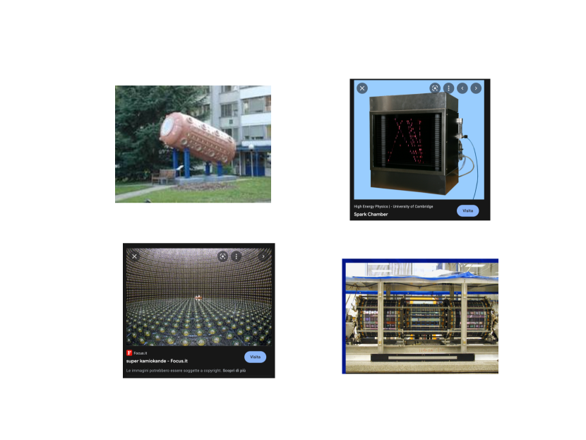
Figure 1: A few examples of quantum measurement devices.

Indeed, independently of the details, a good experimental device faithfully reflects the quantum fluctuations of the system, described by the wave function $|\psi\rangle$. Indeed, the result of each single experiment is, in general, apparently random and unpredictable . Yet, the information encoded in the wave function $|\psi\rangle$ manifests itself as the expectation values for any variable $F$ (and all functions thereof),

$${\bar{F}}\equiv\langle\psi|F|\psi\rangle\;,$$ (1.3)

that is, as a (frequency-) average of the experimental outcomes, ${\bar{f_{n}}}$,

$${\bar{f_{n}}}=\sum_{n}f_{n}\,{\cal P}_{n}\;,\qquad{\cal P}_{n}=|\langle n|\psi\rangle|^{2}\;,$$ (1.4)

where $F|n\rangle=f_{n}|n\rangle$. ${\cal P}_{n}$ is the relative frequency for $f_{n}$. Such a prediction of quantum mechanics is verified by countless experiments. That is, “QM works”.

The prediction (1.4) follows, if one assumes that the probability of each single measurement of $F$ in the state $\psi$ to give $f_{n}$, is given by $P_{n}=|\langle n|\psi\rangle|^{2}\;,$ that is, by Born’s rule. Born’s rule is presented in most textbooks as one of the fundamental postulates of quantum mechanics .

So what is the problem? Well, “the quantum measurement problems”, (a) $\sim$ (i), above!

Throughout, we will denote the (normalized) relative frequency with the calligraphy font ${\cal P}_{n}$, and write the standard probability by using the normal font $P_{n}$. Although they express mathematically the same numbers, they differ conceptually, and lead to distinct logical conclusions.

2 Three aspects of QM

Before analyzing the measurement processes themselves in Sec. 3, we must first discuss briefly three familiar aspects of QM. Though singly well known, clarifying their precise roles in the measurement processes will be essential in the following discussions.

2.1 Expectations values versus Born’s rule

To fix the idea, we consider the system described by the wave function,

$$|\psi\rangle=\sum_{n}c_{n}\,|n\rangle\;,\qquad F|n\rangle=f_{n}|n\rangle\;,\qquad\sum_{n}|c_{n}|^{2}=1\;,$$ (2.1)

where $F$ is the variable we are interested in. Repeated, identical measurement of $F$ will give an average, (1.4).

Now, (1.4) certainly follows from Born’s rule, (1). In other words, the latter is a sufficient condition for the former. The problem is: is Born’s rule also necessary?

The answer is yes, if the following equality holds

$${\bar{O(f_{n})}}\equiv\sum_{n}{\cal P}_{n}O(f_{n})=\langle\psi|O(F)|\psi\rangle\equiv\sum_{n}|c_{n}|^{2}O(f_{n})\;,$$ (2.2)

for general function $O(F)$ of $F$. Then it can be shown that

$${\cal P}_{n}=|c_{n}|^{2}=P_{n}\;.$$ (2.3)

The proof and illustrations are given in [8].

2.2 Pure and mixed states

A system described by a wave function (or a state vector) $\psi$ is a pure state. It contains the complete knowledge of the system.

Otherwise, the system is in a mixed state (or a mixture). It is described by the density matrix, $\rho$.

For instance, a subsystem $A\subset\Sigma$ of a closed system $\Sigma$, described by the wave function,

$$|\Psi\rangle=\sum_{n,\alpha}c_{n,\alpha}|n\rangle|\alpha\rangle\;,\qquad\sum_{n,\alpha}|^{2}=1\;,$$ (2.4)

the expectation value of $G$ (pertinent to the subsystem $A$) is given by

$${\bar{G}}=\langle\Psi|G|\Psi\rangle=\mathop{Tr}\nolimits{\mathbbm{G}}\rho\;,\qquad{\mathbbm{G}}_{mn}\equiv\langle m|G|n\rangle\;,$$ (2.5)

where the density matrix is given in this case by

$$\rho_{nm}\equiv\sum_{\alpha}c_{n,\alpha}c_{m,\alpha}^{*}\;.$$ (2.6)

More generally the density matrix represents any sort of ignorance about the system, and will have forms different from (2.6), but the trace formula

$${\bar{G}}=\mathop{Tr}\nolimits{\mathbbm{G}}\rho\;,$$ (2.7)

is valid always.

2.3 Factorization vis-à-vis entanglement

The question is, symbolically, this: how can we study a single hydrogen atom, an electron, etc., when we know that the wave function involving identical fermions must be antisymmetrized (Fermi-Dirac (FD) statistics)?

The answer is the lack of the spatial support in the wrong component. For instance, for an electron in the laboratory and another in the Sun, the wave function will look like

$$\Psi=\frac{1}{\sqrt{2}}\big{(}\psi_{lab}({\bf r}_{1})\psi_{sun}({\bf r}_{2})-\psi_{lab}({\bf r}_{2})\psi_{sun}({\bf r}_{1})\Big{)}\sim\psi_{lab}({\bf r}_{1})\;,$$ (2.8)

for

$${\bf r}_{1}\in Lab.\;,\qquad{\bf r}_{2}\in Sun$$ (2.9)

as clearly there is no support for the wrong component, $\psi_{lab}({\bf r}_{2})$ or $\psi_{sun}({\bf r}_{1})$.

One sees how a pure state emerges as the result of factorization.

(i)

If the anstisymmetrization is in the spin state, instead of the position states, then the wrong component is negligible, but $\psi_{lab}({\bf r}_{1})$ is in a spin mixed state;

(ii)

If one takes two hydrogen atoms (two electrons) $\sim 2\,m$ apart, in the next room in the laboratory, instead of the second in the Sun, the factorization failure (the effect of the wrong component) is still very small,

$$\sim 10^{-18}\;,$$ (2.10)

as it follows by using Bohr’s radius! And this gives some idea about the exactness of some of our statement below, even if some of the argument about the spacetime localization below concerns spacetime support of the wave functions, rather than the spatial support, considered here.

(iii)

Actually, in spite of the impression this example might have given to the readers, the FD or BE statistics are not fundamental for the purpose of explaining entanglement. Any systems which have interacted in the past are entangled, and in general, in a mixed state.

We note that factorization and entanglement are two faces of the same medal, both characerizing quantum mechanics universally. Note in particular that

• Factorization works remarkably strongly; it makes QM a workable, sensible, physics theory, in spite of the fact that everything is in principle entangled in our universe. It is factorization that makes the pure state a significant concept, both from theoretical and experimental points of view;

• Entanglement leads to the fascinating, characteristic phenomena in QM, such as quantum nonlocality, violation of Bell’s [7] and CHSH [10] inequalities, quantum cryptgraphy, etc. At the same time, the uncontrolled or uncontrollable entanglement with the unobserved systems, is responsible for docoherence, and emergence of classical physics [11]-[16].

A reflection

In principle, we always live in a mixed state: everything is interrelated, and interacted or interacting with each other, in our universe. It is the notion of a pure quantum state, described by a wave function $\psi$, which is extraordinary, and exceptional. They arise as a result of factorization.

These pure states are carefully prepared by experimentalists in many small bubbles in the world, called physics laboratories, equipped with a good clean room and sofiscated (and expensive) vacuum and cryogenic technologies.

But they occur also naturally, on the earth, in the form of radioactivity, which produces $\alpha$ ($\alpha$ particles), $\beta$ (electrons) or $\gamma$ (photons) rays. They also fall from the sky, in the form of cosmic rays (energetic protons, pions, etc.). Then there was light. Light, as it turns out, is a gas of non-interacting, thus, free, photons. They are all pure quantum states.

In a hindsight, we see why these phenomena (providing pure quantum states for free!) have led to the discovery of quantum physics by Planck, at the dawn of the 20th century.

3 The measurement processes

Now we come to our main problem: the quantum measurement processes.

3.1 Effective spacetime localization - state-vector reduction

The measurement of the variable $F$ in the state

$$|\psi\rangle=\sum_{n}c_{n}\,|n\rangle\;,\qquad F|n\rangle=f_{n}|n\rangle\;,$$ (3.1)

is often assumed to proceed as

$$|\psi\rangle\otimes|\Phi_{0}\rangle\otimes|Env_{0}\rangle = \left(\sum_{n}c_{n}|n\rangle\right)\otimes|\Phi_{0}\rangle\otimes|Env_{0}\rangle$$ (3.2)

$$\longrightarrow \left(\sum_{n}c_{n}|n\rangle\otimes|\Phi_{n}\rangle\right)\otimes|Env_{0}\rangle$$ (3.3)

$$\longrightarrow \sum_{n}c_{n}|n\rangle\otimes|\Phi_{n}\rangle\otimes|Env_{n}\rangle\;,$$ (3.4)

where in the first step (3.3) the experimental device reads the measurement results, $f_{n}$, and in the final step (3.4) the “environment” comes be aware of that result (the experimentalist has seen the result on her/his computer screen). These formulas appear to suggest a coherent superposition of distinct macroscopic states leading to paradoxes, debates and endless confusion (the notorious example of this being Schrödinger’s cat “paradox”, see below).

Actually, the factorized form in (3.2)-(3.4), with various $\otimes$ symbols, is not correct, except for the factorization of $|\psi\rangle$ in the first line, namely, before the experiment.

We note that the factorized form $|\Phi\rangle\otimes|Env\rangle$ is incorrect, even before the measurement. The air molecules, the casing of the device, etc., all show that $|\Phi\rangle$ and $|Env\rangle$ are actually entangled. Not only, the boundaries between $|\Phi\rangle$ and $|Env\rangle$ are badly defined, and to be regarded as just a convention. Nevertheless, any experimentalist knows what the relevant part of the device is. She (or he) knows perfectly well that there is no need to push the boundary between the measuring device $|\Phi\rangle$ and the rest of the world $|Env\rangle$ up to inside the human brain, in order to ensure good, precise measurement results.

Keeping this state of matter in mind, we denote the measurement-device-environment entangled “state”, as

$$|\Phi;Env\rangle\;,$$ (3.5)

below. The measurement process can be represented more appropriately as

$$|\psi\rangle\otimes|\Phi_{0};Env_{0}\rangle = \left(\sum_{n}c_{n}|n\rangle\right)\otimes|\Phi_{0};Env_{0}\rangle$$ (3.6)

$$\longrightarrow \sum_{n}c_{n}\,|{\tilde{\Phi}}_{n};Env_{0}\rangle$$ (3.7)

$$\longrightarrow \sum_{n}c_{n}\,|{\tilde{\Phi}}_{n};Env_{n}\rangle\;.$$ (3.8)

where ${\tilde{\Phi}}_{n}$ stands for the entangled state of the microsystem-apparatus with the reading of the measurement result, $f_{n}$. The exact timing of passage from the first stage of measurement-registering of the result on the apparatus (3.7) to the second (3.8) (e.g., the moment in which the experimentalist sees the result on her or his computer screen; others read about it in Physical Review), is entirely immaterial.

Emergence of the mixed state and the state-vector reduction (the “wave function collapse”) occurs as follows.

Just before the measurement, the system is described by a wave function of factorized form by assumption,

$$|\Psi\rangle_{t=0_{-}}=\left(\sum_{n}c_{n}|n\rangle\right)\otimes|\Phi_{0};Env_{0}\rangle\;.$$ (3.9)

The expectation value of any generic variable $G$ in this state (prior to the measurement) is given by

$${\bar{G}}=\langle\Psi|G|\Psi\rangle=\mathop{Tr}\nolimits{\mathbbm{G}}\rho\;,\qquad({\mathbbm{G}})_{mn}\equiv\langle m|G|n\rangle\;,$$ (3.10)

with the density matrix having the form

$$\rho=\left(\begin{array}[]{ccccc}|c_{1}|^{2}&c_{1}c_{2}*&c_{1}c_{3}^{*}&\ldots&\ldots\\ c_{2}c_{1}^{*}&|c_{2}|^{2}&c_{2}c_{3}^{*}&\ldots&\\ c_{3}c_{1}^{*}&&\ddots&&\\ \vdots&&&|c_{n}|^{2}&\\ &&&&\ddots\end{array}\right)\;,$$ (3.11)

characteristic of a pure state, i.e., $\rho_{nm}=c_{n}c_{m}^{*}$. The normalization condition

$$\langle\Phi_{0};Env_{0}|\Phi_{0};Env_{0}\rangle=1\;$$ (3.12)

has been used. In the case of the particular variable $F$ (whose eigenstates are $|n\rangle$’s), ${\mathbbm{F}}$ is diagonal, and its quantum average is given by the known formula

$${\bar{F}}=\mathop{Tr}\nolimits({\mathbbm{F}}\rho)=\sum_{n}f_{n}|c_{n}|^{2}\;.$$ (3.13)

As soon as the microsystem gets into contact with the experimental device, and the measurement events (a chain ionization process, hadronic cascade, etc.) have taken place, the total wave function takes an entangled form, (3.7)

$$|\Psi\rangle_{t=0_{+}}=\sum_{n}c_{n}|{\tilde{\Phi}}_{n};Env_{0}\rangle\;.$$ (3.14)

${\tilde{\Phi}}_{n}$ denotes the entangled microsystem-apparatus state with the reading of the measurement result, $f_{n}$.

Now, the wave function describing ${\tilde{\Phi}}_{m}$ (the aftermath of a measurement, with the result, $F=f_{m}$) and that for ${\tilde{\Phi}}_{n}$ (the aftermath of a measurement, with the result, $F=f_{n}$), corresponding to two distinct spacetime events, have no overlapping spacetime support, as illustrated in Fig. 2. (3.14) is a mixed state.

Treating the formula (3.14) as a mixed state, and not a coherent superposition of states, eliminates at once the contradiction found in a recent paper [17]. The argument of [17] may be regarded as an independent confirmation of the fact that the state after the measurement, (3.14), cannot be a coherent superposition .

The expectation values of a variable $G$ are then given by

$${\bar{G}}=\langle\Psi|G|\Psi\rangle=\sum_{m,n}c_{m}^{*}c_{n}\langle{\tilde{\Phi}}_{m};Env_{0}|\,G\,|{\tilde{\Phi}}_{n};Env_{0}\rangle\;;$$ (3.15)

but the fact ${\tilde{\Phi}}_{m}$ and ${\tilde{\Phi}}_{n}$ ($m\neq n$) have no common spacetime support, means that for any local operator $G$, orthogonality relations,

$$\langle{\tilde{\Phi}}_{m};Env_{0}|\,G\,|{\tilde{\Phi}}_{n};Env_{0}\rangle=0\;,\qquad m\neq n\;,$$ (3.16)

hold. Consequently, ${\bar{G}}$ is given by the sum of the diagonal terms

$${\bar{G}}=\sum_{n}|c_{n}|^{2}G_{nn}\;,\qquad G_{nn}=\langle{\tilde{\Phi}}_{n};Env_{0}|\,G\,|{\tilde{\Phi}}_{n};Env_{0}\rangle\;.$$ (3.17)

This means that the density matrix has been reduced to a diagonal form,

$$\rho=\left(\begin{array}[]{ccccc}|c_{1}|^{2}&&&&\\ &|c_{2}|^{2}&&&\\ &&\ddots&&\\ &&&|c_{n}|^{2}&\\ &&&&\ddots\end{array}\right)\;.$$ (3.18)

For the particular case of the variable $F$, we recover the standard prediction,

$${\bar{F}}=\sum_{n}|c_{n}|^{2}f_{n}\;,\qquad.^{.}.\quad{\cal P}_{n}=|c_{n}|^{2}\;,$$ (3.19)

where ${\cal P}_{n}$ are the normalized relative frequencies for different outcomes $f_{n}$.

The emergence of the mixed state (3.18) is often attributed to the fact that a typical experimental device is made of a macroscopic (difficult-to-specify) number of atoms and molecules, and it is not possible to keep track of the phase relations among different terms in (3.7) to any significant extent.

Also, the macroscopic device $\Phi$, evolving in $t$ entangled with $Env$, can never be in an identical quantum state $|\Phi_{0};Env_{0}\rangle$ at two different measurement instants. This is in stark contrast with the identical quantum state for the microsystem, $|\psi\rangle$, which can be and is indeed produced via e.g., a repeatable experiment (state preparation - see Sec. 3.2) for each measurement.

The observations above are both certainly correct, but we need another, crucial ingredient for the decoherence in the measurement processes: the lack of the common spacetime supports in the wave functions, and the consequent orthogonality and decoherence among terms corresponding to different measurement results, (3.16). Importance of this is that it implies that the result of each measurement event is a state-vector reduction,

$$\left(\sum_{n}c_{n}|n\rangle\right)\otimes|\Phi_{0};Env\rangle\Longrightarrow|{\tilde{\Phi}}_{m};Env\rangle\;:$$ (3.20)

i.e., with a single term present, the instant after the measurement (e.g., with $F=f_{m}$). This state of affair is perceived by us as a “wave-function collapse”.

Summarizing:

A:

The spacetime eventlike nature of the triggering particle-measuring-device interactions introduces an effective spacetime localization of each measurement event;

B:

At the moment the microsystem - a pure quantum state $|\psi\rangle$ - gets into contact with the measurement device-environment state $|\Phi_{0};Env_{0}\rangle$ which is a mixed state, factorization of $|\psi\rangle$ gets lost rapidly, and an entangled, mixed (classical) state $|\Phi_{n};Env_{0}\rangle$ with the unique recording, $F=f_{n}$, is generated.

The result is the state-vector reduction, (3.20).

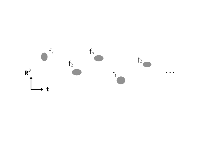
Figure 2: Measurement of a variable $F$. Each blob describes a single measurement event (a chain ionization reaction, hadronic cascade, etc.) occurring at a localized region in spacetime, with the experimental results, $F=f_{7},f_{2},f_{5},f_{1},f_{2}$, etc. The wave functions describing the different measurement events ${\tilde{\Phi}}$ have no overlapping spacetime supports, therefore are orthogonal.

The effective spacetime localization and apparent wave-function collapse, can be nicely visualized in the “double-slit” experiments by Tonomura et. al, [18], see Fig. 3.

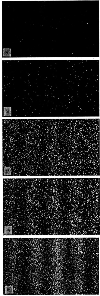
Figure 3: The pictures correspond, from the top to the bottom, to successive exposures to $10$, $100$, $3000$, $20000$ and $70000$ electrons, respectively. Reproduced from [18], A . Tonomura, J . Endo, T . Matsuda, T . Kawasaki and H. Ezawa, “Dimonstration of single-electron buildup of interference pattern”, American Journal of Physics 57, 117 (1989); doi: 10.1119/1.16104, with the permission of the American Association of Physics Teachers.

3.2 Repeatable, nonrepeatable and intermediate types of state reductions

There are actually several types of measurements. The first is known as repeatable, or of the first kind: it proceeds as

$$\left(\sum_{n}c_{n}|n\rangle\right)\otimes|\Phi_{0};Env_{0}\rangle\longrightarrow|m\rangle\otimes|\Phi_{m};Env\rangle\;,$$ (3.21)

which corresponds to the expression often found in a QM textbook,

$$|\psi\rangle=\left(\sum_{n}c_{n}|n\rangle\right)\longrightarrow|m\rangle\;.$$ (3.22)

In these experiments, the measuring device has acquired and recorded the information about the microsystem under observation, but the latter remains unscathed, as a factorized, pure state. These do represent special class of measurements, but they are actually neither rare nor particularly difficult to realize. A variant of the Stern-Gerlach experiment (see Fig. 4) is a good example.

The very possibility of the repeatable measurements is actually of fundamental importance for QM. They allow the preparation of a desired, identical, pure quantum state $|\psi\rangle$ as the initial state, whenever we wish. This is important because in QM the experimental check of the theory is done necessarily with many repeated, identical experiments, as QM predicts only the relative frequencies for various outcomes .

In contrast, a macroscopic body made of, say, $10^{25}$ atoms and molecules (e.g., an experimental device), can never be in an identical quantum state at different times or in different laboratories, even though they might look identical at macroscopic scales. This is in fact one of the underlying reasons for the state-vector reduction (see the discussion above, (3.20)).

The second type of the measurement may be simply termed non repeatable. This is a general type of the measurement - state reduction, as in (3.20). The result $F=f_{m}$ is recorded, but the original microsystem itself (e.g., the electron in Tonomura’s experiment) simply gets lost, in $|{\tilde{\Phi}}_{m};Env\rangle$.

There are also third, intermediate types of measurements. The detection of particle tracks in Wilson, or bubble chambers, or in the silicon vertex detectors, is an example of the measurement of this sort. Note that in these experiments the microscopic particle interacts with the atoms in the devise, generates a local chain ionization cloud, but its information (the position or momentum) does not get lost completely, creating successive ionization clouds (particle tracks) on its way. This kind of processes is particularly important in the momentum or energy measurement.

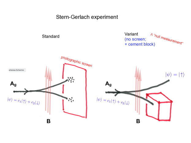
Figure 4: A variant (right) of the standard SG experiment (left). A cement block stops the lower beam containing the spin-down atoms. No measurement is done (known as a “null measurement”), but the atoms coming out of the region consist purely of spin-up state, which can be used as the initial wave function $|\psi(0)\rangle=|\!\uparrow\rangle$.

3.3 Unitarity and linearity

The microscopic state $\psi$

$$|\psi\rangle=\sum_{n}c_{n}|n\rangle\;,$$ (3.23)

if left undisturbed, evolves in time according to the Schrödinger equation,

$$i\hbar\frac{d}{dt}|\psi\rangle=H\,|\psi\rangle\;,$$ (3.24)

($H$ being the Hamiltonian) or as

$$|\psi\rangle\longrightarrow U\,|\psi\rangle=\sum_{n}c_{n}\,U|n\rangle\;,\qquad U=e^{-iHt/\hbar}\;,\quad U^{\dagger}U={\mathbf{1}}\;:$$ (3.25)

it is a linear, unitary evolution. Unitarity means that

$$\langle\psi|\psi\rangle=\sum_{n}|c_{n}|^{2}=1\;,$$ (3.26)

i.e., the state norms are conserved in time. Linearity means (3.25), i.e., superposition of different states in (3.23) continue to be coherent superposition of the corresponding states.

During the measurement process, formally written as (3.7), the time evolution might still look unitary and linear. However, as we have seen, the wave functions associated with different terms in (3.7) do not overlap in spacetime, so it represents actually a mixed state. The coherent superposition of states is no longer there, see (3.16). Most significantly, the real time evolution of the system is the state-vector reduction, (3.20), meaning that linearity in the sense of (3.25) is lost during the measurement.

On the other hand, unitarity is maintained : the sum of all possible outcomes, occurring at different measurements at different times, adds up to unity of the total normalized frequencies, corresponding to the “norm” of the state, (3.7). In terms of the relative frequencies for different outcomes, ${\cal P}_{n}$, unitarity means

$$\sum_{n}{\cal P}_{n}=1\;,\qquad\sum_{n}|c_{n}|^{2}=1\;,$$ (3.27)

even though different (sometimes the same, but repeated) results $f_{n}$ refer to distinct measurements made at different times.

Note that this is indeed how experimentalists view the meaning of unitarity. Unitarity means that ${\cal N}_{n}/{\cal N}$ , to be identified with the theoretical formula, ${\cal P}_{n}=|c_{n}|^{2}$, should satisfy

$$\sum_{n}{\cal N}_{n}/{\cal N}=1\;,$$ (3.28)

which might look trivial. However, this contains an implicit, important assumption that the experimental device has no systematic bias, and registers all possible results $f_{n}$ with equal efficiency and with no losses. Only in such an ideal measurement setting we can expect that the experimental results ${\cal N}_{n}/{\cal N}$ will approach the theoretical prediction, ${\cal P}_{n}$, in the limit of large ${\cal N}$ (e.g., Tonomura’s experiment, Fig. 3).

It might be of some interest to compare the concept of unitarity in the measurement processes as described here, with a more abstract one, in the conventional thinking based on Born’s rule. The latter means in fact

$$\sum_{n}P_{n}=1\;,$$ (3.29)

i.e., that the total probability for a single experiment to give all possible results $f_{n}$, is unity, and that it is conserved in time. The request (3.29), from the mathematical, logical point of view, appears quite indispensable, and indeed has always been considered as a sacrosanct principle in the traditional approach to quantum mechanics.

However, once $P_{n}$ is translated into the physically directly meaningful quantity, ${\cal P}_{n}~{}(=P_{n})$, the expected relative frequencies for various results $f_{n}$ which will be found in distinct measurements and at different times, unitarity as an absolute sacred principle may appear to lose part of the aura surrounding it.

To conclude, one must be cautious in applying the concepts such as linearity or unitarity of the time evolution, valid in the context of (isolated) pure states, to the measurement processes where entanglement between the microsystem and the measurement device as well as with the whole world, plays an essential role. Their consequences in these, complicated mixed states may well (and indeed, do) look differently from what one is accustomed to, from the study of pure quantum states kept in isolation, (3.24), (3.25).

3.4 Measurements, emergence of classical physics, macroscopic quantum states, and models of wave-function collapses

The state after a measurement, $|{\tilde{\Phi}}_{m};Env\rangle$ (in (3.20), is an entangled, classical state, with the recording of the measurement result. The basic reason for that is the so-called envioronment-induced decoherence, studied in [11]-[12]. Emergence of classical physics in this context, is certainly one of the important ingredients in the understanding of the quantum measurement processes (the unique aftermath of each measurement - the wave function collapse).

In author’s view, however, it is useful to consider the whole problem from a wider perspective of what may be called “great twin puzzles of physics today”: the general quantum measurement problems [5]-[7] on the one hand, and emergence of the classical mechanics from QM, on the other. Even though these two classes of the problems are often discussed together [11]-[16], they are actually mostly independent issues . It is better to discuss them separately, and independently. Here we are concerned with the first of them, the general measurement problems; for the second (how Newton’s law emerges from QM), see a recent work, [19].

For instance, we know that sufficiently close to $T=0$, any matter, in any state, is quantum mechanical. At $T=0$ any system is in the unique ground state (Planck-Nernst law, or the first law of thermodynamics).

At $T>0$ but sufficiently close to the absolute zero temperature, a macroscopic body can be in a coherent superposition,

$$|\Psi\rangle=c_{1}|\Psi_{1}\rangle+c_{2}|\Psi_{2}\rangle$$ (3.30)

where $|\Psi_{1}\rangle$ and $|\Psi_{2}\rangle$ are macroscopically distinct states. For experimental efforts to realize macroscopic (or mesoscopic) quantum states at very low temperatures, see [20]-[35].

To talk about the macroscopic quantum states as (3.30) in connection with the measurement problems is, however, slightly out of place. Indeed, the scope of any experimental device is opposite: to acquire the information about the microscopic system $\psi$ under consideration, and to record it in the form of a unique, classical state.

When $|\Psi\rangle$ represents a system with an infinite number of degrees of freedom, there is an exception to the possibility of superposition of (for instance) two, degenerate macroscopic states. The system, at sufficiently low temperatures, will choose one of them as its ground states. It could be tempting to relate such a phenomena of spontaneous symmetry breaking [36, 37] to the wave-function collapse. For instance, one might try to construct a dynamical model [38] of spin $1/2$ particle, interacting with a doubly degenerate (2D) Ising model ground states, so as to mimic the state-vector reduction, (3.20).

More generally, the Ising model system may be replaced by some classical “pointer” states; the idea is to construct a model of nonunitary evolution of the microsystem $\psi$ coupled to the pointer, to reproduce effectively (3.20), with correct relative frequencies for different outcomes .

Whether or not such a model of the wave-function collapse can be successfully constructed eventually, the conclusion from our discussion in this section (and in [8]) is the following:

No dynamical models of wave-function collapse are needed.

In our view, “wave-function collapse” is one of the worst misnomers in the quantum mechanics discussions. The words evoke in our mind a mysterious, nonlinear evolution which shrinks almost instantaneously whatever distribution present in $\psi$ before the measurement. No such processes exist. Every experimentalist knows what happens in each measurement: they are chain-ionizations and amlification, hadronic cascades in a calorimeter, recording of the particle tracks, etc. They represent all nonadiabatic, irreversible processes. However complicated in detail, they are all processes we understand well in principle, in terms of the standard theory of the fundamental interactions [1]-[4].

The state reduction (3.20) is just the way we perceive the fact that the result of each measurement is necessarily one of the terms in (3.7). The wave functions of the states of the microsystem-device coupled system, corresponding to different measurements, have no common spacetime support, hence the wave function apparently - only apparently - “collapses”.

4 Three puzzles

Before concluding, let us go through quickly three familiar puzzles and their resolution.

4.1 Quantum jumps versus Schrödinger’s equation

A question often debated is how to reconcile the smooth time evolution of the wave function described by the Schrödinger equation with sudden “quantum jumps”, occurring in radioactive nuclei ($\alpha$ and $\beta$ decays), or in atoms in excited states, and so on.

Let us consider an $\alpha$ decay from a metastable nucleus, $X$,

$${}^{A}_{N}\left(X\right)\Longrightarrow{}^{A-4}_{N-2}\left(Y\right)+\alpha\;,$$ (4.1)

where $N$ is the atomic number and $A$ is the mass number. The wave function for the system may be written as

$$|\psi\rangle=|X\rangle+|Y\rangle|\alpha\rangle\;.$$ (4.2)

We do not bother to write the coefficients in front of the two terms: their norms are not conserved due to the decay. The first ($|X\rangle$) corresponds to a bound state; the second ($|Y\rangle|\alpha\rangle$) an unbounded system. The interference between them is absent. (4.2) is not the wave function of a pure state. It is a mixed state.

The state being metastable, its energy has a small imaginary part,

$$E=E_{R}-i\,\frac{\Gamma}{2}\;,$$ (4.3)

where $\Gamma$ represents the total decay rate per unit time (or the level width), and $\tau=\hbar/\Gamma$ is the mean lifetime. The wave function has a time dependence (for instance, see [40]),

$${\tilde{\psi}}_{X}(t)=e^{-iEt/\hbar}{\tilde{\psi}_{X}(0)}=e^{-iE_{R}t/\hbar}e^{-\Gamma t/2\hbar}{\tilde{\psi}_{X}(0)}\;.$$ (4.4)

Now how can one reconcile such a smooth time dependence with sudden quantum jumps, such as $\alpha$ decay, a spontaneous emission of photons from an excited atom? This sort of question, probably mixed up with a philosophical confrontation between Heisenberg’s view (based on the matrix mechanics, for the transition elements) and Schrödinger’s one (with a smooth differential equations) of quantum mechanics, dominated the earlier debates on quantum mechanics .

Actually, from the very way the wave function $\tilde{\psi}$ for a metastable state is defined, where $\Gamma$ represents the total decay rates of all possible decay processes of the parent particle, it is quite clear that $\tilde{\psi}$ represents an effective description of the metastable “quantum state”, in which the coarse-grained time dependence (decay events) has been smoothed out. It does not have the same status as the wave function of a genuine quantum state $\psi$.

In conclusion, the conundrum of apparent impossibility of reconciling the smooth time-dependent Schrödinger equation with quantum jumps, appears to have been caused by the confusion between the concept of the true wave function $\psi$ and that of an effective “wave function” for a metastable “state”, ${\tilde{\psi}}$.

See [8] for more discussions.

4.2 Schrödinger’s cat

In the discussion involving Schrödinger’s cat, the initial “wave function” is a combination (4.2), between the undecayed nucleus $|X\rangle$ and the state after decay, $|Y\rangle|\alpha\rangle$. To maximally simplify the discussion, let us eliminate altogether the intermediate, diabolic device which upon receipt of the $\alpha$ particle leads to the poisoning of the cat, and treat the cat directly as the measuring device, $|\Phi\rangle$. When it detects the $\alpha$ particle, it dies; when it does not, it remains alive. There are two terms in the measurement process, (3.6), (3.7), which here reads

$$|\psi\rangle\otimes|\Phi_{0}\rangle=\left(|X\rangle+|Y\rangle|\alpha\rangle\right)\otimes|\Phi_{0}\rangle$$ (4.5)

$$\longrightarrow |X\rangle\otimes|\Phi^{(alive)}\rangle+|Y\rangle|\alpha\rangle\otimes|\Phi^{(dead)}\rangle\;$$ (4.6)

(we dropped also the rest of the world, $|Env\rangle$). Such a process appears to lead to the superposition of the dead and alive cat, which is certainly an unusual notion, difficult to conceive, to say the least.

Actually, there are some abuse and/or misuse of concepts in this argument, each of which individually invalidates it, eliminating the notorious conundrum.

The first is the fact, as seen in the last section, that the “state” of the undecayed nucleus, $X$, is not a pure state. The “wave function” ${\tilde{\psi}}_{X}$ describing it is not a proper wave function but an effective one, in which the coarse-grained time dependence has been averaged out. Second, the linear superposition $|\psi\rangle\sim|X\rangle+|Y\rangle|\alpha\rangle$, as discussed around (4.2), does not represent a pure state, but a mixed state: $|Y\rangle|\alpha\rangle$ represents the decay product of $|X\rangle$, unbounded and incapable of interfering with the latter.

Finally, even putting aside these two issues, the process (4.5), (4.6) has clearly all the characteristics of a general measurement process discussed in Sec. 3. As explained there, the wave functions describing the two terms of (4.6) lack overlapping spacetime supports. There are no interferences between the terms involving the coupled system involving the microsystem and the classical measurement device (the cat here). The formula (4.6) represents a mixture.

Equivalently, and perhaps more intuitively, one can use the notion of the wave-function collapse. The exact timing of the spontaneous $\alpha$ decay cannot be predicted, as it reflects a quantum fluctuation. But the moment an $\alpha$ particle is emitted, and the cat gets hit by it (the instant of the measurement), the wave function collapses,

$$|\psi\rangle\otimes|\Phi_{0}\rangle\Longrightarrow|Y\rangle|\alpha\rangle\otimes|\Phi^{(dead)}\rangle\;.$$ (4.7)

Recapitulating, Schrödinger’s cat paradox, was caused by improper use of concepts such as the superposition principle, unitary and linearity of evolution, and by mixing up the pure and mixed states .

Setting aside these arguments, the idea of superposition of dead and alive cat states, represents in itself a self-contradictory, impossible notion. A macroscopic superposition of states such as (3.30) or (4.6), requires the body temperature of the system close to $T=0$, whereas a living cat needs room (body-) temperatures for its biological functions: it is necessarily a mixed state [19].

4.3 Quantum entanglement, quantum nonlocality and EPR paradox

Let us consider now the famous Einstein-Podolsky-Rosen setting (in Bohm’s version) of a total spin $0$ system decaying into two spin $\tfrac{1}{2}$ particles flying away from each other. The (spin) wave function is given by

$$|\Psi_{0}\rangle=\frac{1}{\sqrt{2}}\left(|\!\uparrow\rangle|\!\downarrow\rangle-|\downarrow\rangle|\!\uparrow\rangle\right)$$ (4.8)

​ where $|\!\uparrow\rangle$ ($|\!\downarrow\rangle$) represents the state of the 1st and 2nd spins, $s_{1,z}=\pm\tfrac{1}{2}$, $s_{2,z}=\pm\tfrac{1}{2}$. As spin components of the single spins do not commute with the total spin ${\mathbbm{S}}_{tot}^{2}$, e.g.,

$$[{\mathbbm{S}}_{tot}^{2},s_{1,i}]\neq 0\;,\quad[{\mathbbm{S}}_{tot}^{2},s_{2,j}]\neq 0\;,\qquad i,j=x,y,z\;,$$ (4.9)

$s_{1\,z},s_{2\,y}$, etc., are fluctuating between $\pm\tfrac{1}{2}$ in the state $\Psi_{0}$. Note that $\Psi_{0}$ can be written in infinitely many different ways, reflecting possible fluctuation modes of the subsystems,

$$|\Psi_{0}\rangle=\frac{1}{\sqrt{2}}\left(|+\rangle|-\rangle-|-\rangle|+\rangle\right)=\frac{1}{2}\left[\,|\!\uparrow\rangle(|+\rangle-|-\rangle)-(|+\rangle-|-\rangle)|\!\uparrow\rangle\,\right]=\ldots\;.$$ (4.10)

It is of fundamental importance to realize that such (correlated) fluctuations of the two subsystems - quantum entanglement - are present however distant the subsystems may be, and even if they are relatively spacelikely separated. Nothing in $\Psi_{0}$ tells us otherwise. Nothing in quantum mechanical law says that such entanglements are present only when the subsystems are nearby, e.g., less than $10^{-8}$ cm, or less than $10^{+28}$ cm. Simply,

Quantum mechanics does not contain any fundamental parameter with the dimension of a length .

In the EPR-Bohm experiment, this means that an experimental result at one arm, say, $s_{1\,z}=\tfrac{1}{2}$, might appear to imply “instantaneously” that the second experiment at the other arm would be in the state $s_{2\,z}=-\tfrac{1}{2}$, even before it is actually performed, and however distant they may be. This could sound paradoxical (sometimes the term “quantum nonlocality” is used). The second experimentalist, not having access to the first experiment, might have (should have?) expected to find the results $s_{2\,z}=\pm\tfrac{1}{2}$, a priori with equal probabilities.

This kind of argument has led to the introduction of the hidden-variable hypothesis (see [7] for discussions), although such a deduction was not really justified. We limit ourselves here to noting that this argument had logical flaws. First, the contemporaneity of the two experiments is not really an issue: the experimentalists must just ensure that they are studying the two spin $\tfrac{1}{2}$ particles from the same decay event - the coincidence check. The exact time ordering, which depends on the reference system chosen, cannot matter. In any case, as the two subsystems are spacelikely separated, it is untrue that the second experimentalist would know instantaneously the result of the first experiment, or actually, even whether or not the first measurement has been indeed performed. The information transmission is itself a dynamical process. Finally, the two “simultaneous” experiments would capture only those states of the two subsystems fluctuating according to the entangled wave function, (4.8), (4.10). In conclusion, for the second experimentalist the system presents itself as a mixture with an unknown density matrix. He (she) simply does not know what to expect. Therefore there was no paradox, whatsoever.

It is true that the first experimental result $s_{1\,z}=\tfrac{1}{2}$ does imply, instantaneously (whatever it may mathematically mean), that the other spin is in the state $|{\downarrow}\rangle=\tfrac{1}{\sqrt{2}}(|+\rangle-|-\rangle)$, as is seen from the wave function (4.8), (4.10). This quantum nonlocality, just a name for this particular aspect of quantum entanglement, is real. It should, however, not be confused with the dynamical concept of locality (or causality) . Quantum mechanics is perfectly consistent with causality and locality, due to the fact that all the fundamental, elementary interactions are local interactions in spacetime (see [8] and [42]). No dynamical effects, including the information transmission, propagate faster than the velocity of light. It is perhaps best to regard (4.8) simply as a particular kind of macroscopic quantum-mechanical state.

It is essential to realize that, unless the second measurement is done, any components of the second spin other than $s_{2\,z}$ are still fluctuating . Thus if the two Stern-Gerlach type experiments are performed at the two ends simultaneously, by using the magnets directed to generic directions ${\bf a}$ and ${\bf b}$, they would find, experiment by experiment, apparently random results, such as $(s_{1\,a},s_{2\,b})=(\tfrac{1}{2},\tfrac{1}{2}),(\tfrac{1}{2},-\tfrac{1}{2}),(-\tfrac{1}{2},-\tfrac{1}{2})$, etc. But their fluctuation average is encoded in $\Psi_{0}$:

$$\langle\Psi_{0}|s_{a}s_{b}|\Psi_{0}\rangle=-\frac{1}{4}\cos\theta_{a,b}=-\frac{1}{4}\,{\bf a}\cdot{\bf b}\;.$$ (4.11)

A possible way to discriminate between any alternative theory with hidden variables from quantum mechanics, has been mathematically formulated, e.g., in the form of the Bell [7], or CSHS [10] inequalities for analogous, polarization correlated photon pair experiments. Beautiful experiments by Aspect et. al. (1981) [43] have subsequently demonstrated that, whenever the hidden-variable alternatives and quantum mechanics give discrepant predictions (for certain sets of polarizer axes), the experimental data confirm quantum mechanics, disproving the former.

See also Chiao et. al. (1995) [44] for a series of related experiments and discussions on quantum nonlocality. See [40, 8] also for comments on and resolution to Mermin’s conundrum [45] in systems with entanglement among more than two particles.

A reflection

As reviewed in Sec. 2.3, quantum correlations (entanglement) among the particles whose positions are space-like-ly separated, and hence are no longer capable to communicate with, or dynamically influence on, each other, as the two spin $1/2$ particles in (4.8), (4.10), are quite a common, ordinary and ubiquitous phenomenon in QM. What is not quite ordinary, is that this “quantum nonlocality” does not represent any violation of dynamical causality or locality (sometimes called Einstein causality). Quantum mechanics is rigorously consistent with this principle, even though the proof of this fact requires working in the framework of relativistic quantum field theory, quantum theory of particles [8, 42].

Now how can these two, apparently contradicting properties of quantum mechanics coexist peacefully within the same theory? The answer lies in another fundamental aspect of QM: the wave function is not itself a measurable physical quantity (an observable). Only the relative frequencies for different outcomes (probabilities) are predicted by it.

In hidden-variable models, the statistical aspect of quantum mechanics is replaced by a classical statistical (unknown) distribution of the hidden parameters $\{\lambda\}$, complementing the standard description with the wave function. But once the value(s) of $\{\lambda\}$ at $t=0$ is (are) chosen, all possible imaginable future experimental outcomes are determined uniquely (i.e., classical evolutions).

A hidden-variable theory, with a logical structure so sharply different from that of quantum mechanics, cannot reproduce all of the predictions of the latter. It could, actually, if one is willing to introduce nonlocal, noncausal evolutions. This is seen clearly, e.g., in the unphysical, noncausal behavior of the trajectory $X(t)$ in Bohm’s pilot-wave theory [7],[40] which is a particular type of hidden-variable model, designed by construction to reproduce all QM predictions.

If we insist, instead, that a hidden-variable model must respect local causality, then its predictions necessarily satisfy certain inequalities such as those in [7], [10]. Bell and Clauser et. al. have shown that some predictions of QM should lie outside such a bound, a fact verified, in a dramatic experimental confirmation of QM [43].

5 Conclusion

Here are the answers to the “quantum measurement problems” enlisted in the beginning:

(a)

Wave function collapse?

No. See the Summary A. and B. after Eq. (3.20), and the discussion at the end of Sec. 3.4;

(b)

Macroscopic superposition of states?

Yes (at temperatures close to $T=0$ and without environment-induced decoherence); No, otherwise;

(c)

Forever branching manyworlds tree?

No;

(d)

Spontaneous collapse of micro state, of the experimental device, and of the world?

No;

(e)

Wave function just a bookkeeping device?

No;

(f)

Quantum jumps vs Schrödinger equation?

Explained, see Sec. 4.1;

(g)

Born’s rule from the Schrödinger equation involving everything?

Yes, but only effectively. No, as a result a complicated nonlinear dynamical process. See the Summary A. and B. after Eq. (3.20);

(h)

Quntum nonlocality?

Yes, see the discussions in Sec. 4.3;

Hidden variables?

No. See the “reflection” at the end of Sec. 4.3.

(i)

Is it possible that the fundamental, complete theory of physics is incapable of unique prediction for a single measurement?

Yes.

The key observation of this work that the basic entities (the degrees of freedom) of our world are various types of particles, leads to the idea that each measurement, at its core, is a spacetime, pointlike event. The crux of the absence of coherent superposition of different terms in the measuring process (3.7) is, indeed, the consequent lack of the overlapping spacetime supports in the associated wave functions, instant after measurement which is the process of entanglement between the microsystem and the experimental device and the environment. It is in this sense the expression (3.7) represents a mixed state. But it also implies that the aftermath of each measurement corresponds to a single term of (3.7). This (also empirical) fact, is known as the “wave-function collapse”, or the state-vector reduction.

The discussions of Sec. 3 have led to the diagonal density matrix, (3.18). In particular, the information encoded in the wave function $|\psi\rangle=\sum_{n}c_{n}|n\rangle$ has been transferred via entanglement with the experimental device and environment into the relative frequencies for finding the experimental results $F=f_{n}$, ${\cal P}_{n}=|c_{n}|^{2}$. Combined with the equality between ${\cal P}_{n}=|c_{n}|^{2}$ (the relative frequencies) and $P_{n}=|c_{n}|^{2}$ (the probabilities) [8] our results represent the first steps towards filling in the logical gaps in Born’s rule, by explaining the state-vector reduction, and pointing towards a more natural interpretation of quantum mechanics.

Our discussions do confirm the standard Born rule as a concise way of summarizing the predictions of quantum mechanics. But the fact that the latter is formulated in terms of the “probability certain result is found in an experiment, which might (or might not) be eventually performed - perhaps by an experimentalist with a Ph D - has always caused confusion and conceptual difficulties .

In ultimate analysis, the problem of Born’s rule is the fact that it presumes a human intervention.

We instead take the quantum fluctuations described by the wave function as real, and propose that they represent the fundamental laws of quantum mechanics. They are there, independently of any experiments, and in fact, whether or not we human beings are around .

What we propose here is a slightly unconventional way of understanding quantum mechanical laws. Indeed, the solid textbook materials and the standard methods of analysis in quantum mechanics, all remain unchallenged. After all, we know that quantum mechanics is a correct theory.

The new perspective, however, suggests us to dispense with, in the discussion of quantum mechanics, certain familiar concepts such as probability, statistical ensembles, Copenhagen interpretation, etc., which historically have guided us, but also caused misunderstandings and introduced clouds in the discussion on quantum mechanics, for many years.

Accepting the quantum fluctuations described by the wave function as real, we simply give up pretending, or demanding, that in a fundamental, complete theory describing Nature the result of each single experiment should necessarily be predictable.

As cosmologists tell us today, all the known structures of our universe (including galaxies, stars, planets and ourselves) are believed to have grown out of uncontrollable quantum density fluctuations at some stage of the inflationary universe. In other words:

God may not play dice, but Nature apparently does.

We believe that our new, clearer understanding the quantum mechanical laws of Nature, has far-reaching consequences and applications in all present and future science domains in physics and beyond, from biology and chemistry, quantum information and quantum computing, and possibly, to the brain science.

We thank the organizers and participants of the DICE2022 conference, Castiglioncello (Rosignano Marittimo, Tuscany), Sept. 19-23, 2022, where this talk was presented, for a stimulating atmosphere. A special gratitude is reserved to Hans-Thomas Elze, for the kind invitation and for many fruitful discussions. The author’s work is supported by an INFN special initiative grant, GAST (Gauge and String Theories).

References

References

- [1] Weinberg S 1967 “A model of Leptons”, Phys. Rev. Lett. 19, 1264
- [2] Salam A Weak and electromagnetic interactions “Elementary Particle Theory”, ed. N. Svartholm, Almqvist Forlag AB, 367 (1968).
- [3] Glashow S L, Iliopoulos J, Maiani L 1970 “Weak Interactions with Lepton-Hadron Symmetry,” Phys. Rev. D 2, 1285 (1970).
- [4] Fritzsch H, Gell-Mann M, Leutwyler H 1973 ”Advantages of the color octet gluon picture”, Physics Letters 47 B (1973), 365
- [5] Wheeler J A, Zurek W H 1983 Quantum Theory and Measurement (Princeton University Press)
- [6] Peres A 1995 Quantum Theory: Concepts and Methods (Dordrecht/Boston/London: Kluwer)
- [7] Bell J S 1987 Speakable and unspeakable in quantum mechanics (Cambridge University Press)
- [8] Konishi K 2022 Quantum fluctuations, particles and entanglement: a discussion towards the solution of the quantum measurement problems,” Int. Journ. Mod. Phys. A 37, (2022) 2250113 [arXiv:2111.14723 [quant-ph]]
- [9] Dirac P A M 1958 Principles of Quantum Mechanics (Oxford University Press)
- [10] Clauser J F, Horne M A, Shimony A, Holt R A 1969 “Proposed experiment to test local hidden-variable theories”, Phys. Rev. Lett., 23 (15) 880
- [11] Zurek W H 2003 “Decoherence, einselection, and the quantum origins of the classical,” Rev. Mod. Phys. 75, 715-775 doi:10.1103/RevModPhys.75.715 [arXiv:quant-ph/0105127 [quant-ph]]
- [12] Joos E, Zeh H D, Kiefer C, Giulini D, Kupsch J, Stamatescu I O 2002 Decoherence and the Appearance of a Classical World in Quantum Theory (Springer)
- [13] Joos E, Zeh H D 1985 “The emergence of classical properties through interaction with the environment”, Z. Phys. B 59, 223-243
- [14] Zurek W H 1991 “Decoherence and the Transition from Quantum to Classical”, Physics Today 44, 10, 36, https://doi.org/10.1063/1.881293
- [15] Tegmark M 1993 “Apparent wave function collapse caused by scattering,” Found. Phys. Lett. 6, 571 doi:10.1007/BF00662807 [arXiv:gr-qc/9310032 [gr-qc]]
- [16] Zurek W H 2003 “Decoherence, einselection, and the quantum origins of the classical,” Rev. Mod. Phys. 75, 715-775 doi:10.1103/RevModPhys.75.715 [arXiv:quant-ph/0105127 [quant-ph]]
- [17] Frauchiger D, Renner R 2018 “Quantum theory cannot consistently describe the use of itself”, Nature Communications 9, 3711
- [18] Tonomura A, Endo J, Matsuda T, Kawasaki T, Ezawa H, 1989 “Dimonstration of single-electron buildup of interference pattern”, American Journal of Physics 57 117
- [19] Konishi K 2022 “Newton’s equations from quantum mechanics for macroscopic bodies in the vacuum”, Preprint [arXiv:2209.07318 [quant-ph]]
- [20] Leggett A J 1980 “Macroscopic Quantum Systems and the Quantum Theory of Measurement”, Suppl. of the Progress of Theoretical Physics 69 80
- [21] Arndt M, Nairz O, Vos-Andreae J, Keller C, van der Zouw G, Zeilinger A 1999 “Wave-particle duality of molecules”, Nature 401 680
- [22] O’Connell A D, et. al., 2010 “Quantum ground state and single-photon control of a mechanical resonator”, Nature, 464 (7289) 697
- [23] Arndt M, Hornberger K 2014 “Testing the limits of quantum mechanical superpositions”, Nature Physics 10 271 [arXiv:1410.0270v1 [quant-ph]]
- [24] Courty J M, Heidmann A, Pinard M 2001 “Quantum limits of cold damping with optomechanical coupling”, Eur. Phys. J. D 17, 399–408
- [25] Armour A D, Blencowe M P, Schwab K C 2002 “Entanglement and decoherence of a Micromechanical Resonator via Coupling to a Cooper-Pair Box”, Phys. Rev. Lett. bf 88 148301
- [26] Knobel R G, Cleland A N 2003 “Nanometre-scale displacement sensing using a single electron transistor”, Nature, 424 17
- [27] LaHaye M D, Buu O, Camarota B, Schwab K C 2004 “Approaching the Quantum Limit of a Nanomechanical Resonator”, Science 304, 74
- [28] Cleland A N, Geller M R 2004 “Superconducting Qubit Storage and Entanglement with Nanomechanical Resonators”, Phys. Rev. Lett. 93 070501
- [29] Martin I, A. Shnirman I A, Tian L, Zoller P 2004 “Ground-state cooling of mechanical resonators”, Phys. Rev. B 69, 125339
- [30] Kleckner D, Bouwmeester D 2006 “Sub-kelvin optical cooling of a micromechanical resonator”, Nature, 444 2
- [31] Regal C A, Teufel J D, Lehnert K W 2008 Measuring nanomechanical motion with a microwave cavity interferometer (Macmillan Publishers Limited) doi:10.1038/nphys974
- [32] Schliesser A, Rivière R, Anetsberger G, Arcizetandt O, Kippenberg J 2008 Resolved-sideband cooling of a micromechanical oscillator (Macmillan Publishers Limited) doi:10.1038/nphys939
- [33] Abbott B et al. [LIGO Scientific] 2009 “Observation of a kilogram-scale oscillator near its quantum ground state,” New J. Phys. 11, 073032 doi:10.1088/1367-2630/11/7/073032
- [34] O’Connell A D, et. al. 2010 “Quantum ground state and single-photon control of a mechanical resonator”, Nature, 464 (7289) 697
- [35] Brand C, Troyer S, Knobloch C, Cheshinovsky O, Arndt M A (2021) Single, double and triple-slit diffraction of molecular matter waves Preprint arXiv:2108.06565v2 [quant-ph]
- [36] Nambu Y, Jona-Lasinio G 1961 “Dynamical Model of Elementary Particles Based on an Analogy with Superconductivity. I”, Physical Review 122: 345, “Dynamical Model of Elementary Particles Based on an Analogy with Superconductivity. II”, Physical Review 124: 246
- [37] Goldstone J 1961 ”Field theories with ”superconductor” solutions”. Il Nuovo Cimento. 19 (1) 154
- [38] Allahverdyan A E, Balian R, Nieuwenhuizen T M 2013 “Understanding quantum measurement from the solution of dynamical models”, Phys. Rep. 525 1-166 arXiv:1107.2138
- [39] Fröhlich J 2020 A Brief Review of the ETH-Approach to Quantum Mechanics In: Anantharaman N., Nikeghbali A., Rassias M.T. (eds) Frontiers in Analysis and Probability (Springer, Cham)
- [40] Konishi K, Paffuti G 2009, Quantum Mechanics: A New Introduction (Oxford University Press)
- [41] Tomonaga S 1968 Quantum Mechanics Vol. II, (North Holland)
- [42] Peskin M E, Schröder D V 1995 An Introduction to Quantum Field Theory (New York, Addison-Wesley)
- [43] Aspect A, Grangier P, Roger G 1981 “Experimental realization of Einstein-Podolsky-Rosen-Bohm Gedankenexperiment: A new violation of Bell’s inequalities”, Phys. Rev. Lett. 49 91
- [44] Chiao R Y, Kwiat P G, Steinberg A M 1995 Quantum Nonlocality in Two-Photon Experiments at Berkeley Preprint arXiv:quant-ph/9501016, and references therein
- [45] D. Mermin D (1990) “Quantum mysteries revisited”, American Journal of Physics, 58, 731