Model-independent measurement of cosmic curvature with the latest $H(z)$ and SNe Ia data: A comprehensive investigation

Abstract

In the context of the discrepancies between the early and late universe, we emphasize the importance of independent measurements of the cosmic curvature in the late universe. We present an investigation of the model-independent measurement of the cosmic curvature parameter $\Omega_{k}$ in the late universe with the latest Hubble parameter $H(z)$ measurements and type Ia supernovae (SNe Ia) data. For that, we use two reconstruction methods, the Gaussian process (GP) and artificial neural network (ANN) methods, to achieve the distance construction from $H(z)$ data. Our analysis reveals that the GP method provides the most precise constraint on $\Omega_{k}$, with a constraint precision of $\xi(\Omega_{k})=0.13$, surpassing recent estimations using similar methods. The GP method consistently indicates a preference for a flat universe at the 2$\sigma$ confidence level. Moreover, we find that the choice of reconstruction method influences the estimation of $\Omega_{k}$. The ANN reconstruction method exhibits higher sensitivity to the addition of BAO $H(z)$ data, resulting in comparable constraint precision to the GP method. A discrepancy exists between the best-fit values obtained by these two reconstruction methods, indicating their dependence on the reconstruction approach. However, we anticipate that with the improvement of sample size and precision of observational $H(z)$ data, the estimation of $\Omega_{k}$ using this approach will become more robust and reliable.

I Introduction

After nearly a century of cosmological research, a standard cosmological model, the $\Lambda$ cold dark matter ($\Lambda$CDM) model with six base parameters, was established, whose validity has been verified by almost all current observational data (Riess et al., 1998; Perlmutter et al., 1999; Spergel et al., 2003; Tegmark et al., 2004; Abazajian et al., 2004), especially by the Planck-satellite data with breathtaking precision (Ade et al., 2016; Aghanim et al., 2020). However, as the precision of the observational data increases, some anomalies among different measurements of some key cosmological parameters are shaking our confidence in the standard cosmological model (Riess et al., 2019; Aghanim et al., 2020; Qi et al., 2021, 2022; Cao et al., 2022; Di Valentino et al., 2019, 2021a; Handley, 2021). The most compelling ones appear to be the tension of the Hubble constant $H_{0}$ between the value inferred from the Planck-satellite data and the one inferred from the nearby type Ia supernovae (SNe Ia) data calibrated by the distance ladder, which has become a serious crisis for cosmology (Riess et al., 2021; Di Valentino et al., 2021b; Vagnozzi, 2020; Zhang, 2019; Xu and Zhang, 2020; Li et al., 2013; Qi and Zhang, 2020; Vattis et al., 2019; Zhang et al., 2014a; Guo et al., 2019; Zhao et al., 2017; Guo and Zhang, 2017; Gao et al., 2021, 2022). As far as the second anomaly is concerned, the $S_{8}$ parameter, a combination of the amplitude of matter density fluctuations and the matter density, is significantly lower in recent cosmic shear surveys than that expected according to the Placnk data best fit $\Lambda$CDM model (Heymans et al., 2021).

In addition, recently, an enhanced lensing amplitude in cosmic microwave background (CMB) power spectra from Planck 2018 data also presents another serious challenge to the standard cosmological model (Aghanim et al., 2020; Handley, 2021; Di Valentino et al., 2019). This effect could be explained naturally by a closed universe. However, the prevailing and very successful inflationary theory predicts a flat universe, and the observations also support a flat universe. For instance, the combination of CMB power spectra data and baryon acoustic oscillation (BAO) data puts a stringent constraint on the cosmic curvature parameter $\Omega_{k}$ under $\Lambda$CDM, strongly supporting a flat universe (Spergel et al., 2003; Ade et al., 2016; Aghanim et al., 2020; Stevens et al., 2023). As a result, most cosmological research has long assumed a flat universe. However, the discovery of a closed universe at more than 3.4$\sigma$ confidence level, preferred by the enhanced lensing amplitude in Planck 2018 data, suggests that this assumption may not be taken for granted (Di Valentino et al., 2019; Handley, 2021). What is worse is that the $H_{0}$ and $S_{8}$ tensions will be exacerbated when the possibility of a closed universe is considered, implying there may be even larger discordances hidden behind the assumption of a flat universe (Di Valentino et al., 2019, 2021a). For a comprehensive and detailed discussion on this topic, we recommend readers to refer to Refs. (Efstathiou and Gratton, 2020; Vagnozzi et al., 2021a, b; Gonzalez et al., 2021; Zuckerman and Anchordoqui, 2022; Akarsu et al., 2023; Glanville et al., 2022; Bel et al., 2022; Stevens et al., 2023; Favale et al., 2023; Cao et al., 2021; Zhai et al., 2020; Ryan et al., 2019; Park and Ratra, 2019; Penton et al., 2018; Ryan et al., 2018; Yu et al., 2018).

In fact, all of these crises arise from the measurement inconsistencies between the early and late universe, and point to the fact that the cracks have appeared in the standard $\Lambda$CDM model. It is time to reconfirm what we once knew for sure. In this paper, we aim to thoroughly investigate whether the spatial geometry of our universe is open, flat, or closed with a cosmological model-independent method. This is not only in response to the crisis mentioned above but also because the spatial curvature of the universe is a significant issue that is deeply relevant to many fundamental questions in modern cosmology, such as the evolution of the universe and the property of the dark energy. The spatial geometry of the universe is usually described by the cosmic curvature parameter $\Omega_{k}$, i.e., $\Omega_{k}>0$, $\Omega_{k}=0$ and $\Omega_{k}<0$ correspond to an open, flat, and closed universe, respectively. In order to tackle the crisis arising from the measurements of cosmic curvature, a necessary approach is to use a cosmological model-independent method to confirm the value of $\Omega_{k}$ in the late universe. Recently, great progress has been made in this regard.

So far, many cosmological model-independent methods have been proposed to determine the cosmic curvature parameter $\Omega_{k}$ (Collett et al., 2019; Qi et al., 2021; Wang et al., 2021, 2020a; Clarkson et al., 2007, 2008; Wang et al., 2020b; Xia et al., 2017; Cai et al., 2016), in which a popular and effective method is applying the distance sum rule in the combination of strong gravitational lensing (SGL) and SNe Ia observations to constrain $\Omega_{k}$ (Räsänen et al., 2015). Subsequently, this method has been fully implemented with the combination of SGL and other distance indicators, such as intermediate luminosity quasars and gravitational waves (Wang et al., 2022; Qi et al., 2021, 2022; Cao et al., 2022). However, while it is true that this method is independent of cosmological models, Qi et al. (Qi et al., 2019) found that it is dependent on the mass distribution model of lens galaxies and is also affected by the classification of SGL data according to the lens velocity dispersion. To obtain an unbiased and precise estimate $\Omega_{k}$ in this way, it is crucial to accurately characterize the mass distribution of lens galaxies for each SGL sample, but this is still a long way off.

Another popular model-independent method to determine $\Omega_{k}$ is originally proposed to test the homogeneous and isotropic Friedmann-Lemaître-Robertson-Walker (FLRW) metric (Clarkson et al., 2008). This method is derived from the theoretical expression between cosmological distance and the Hubble parameter $H(z)$, in which the cosmic curvature is involved. In reverse, the cosmic curvature could be estimated under the assumption of the FLRW metric. Subsequently, this estimation of $\Omega_{k}$ is implemented in several works in the light of new data and different statistical methods (Wei and Wu, 2017; Yu and Wang, 2016; Dhawan et al., 2021). In most of these works, the Gaussian process, a non-parametric reconstruction technique, is widely used to reconstruct a smooth curve of $H(z)$ so that the distance at any redshift can be calibrated. Recently, Wang et al. (Wang et al., 2020a, 2021) presented an alternative non-parametric approach based on the artificial neural network (ANN) for reconstructing a function from observational data, which also has been used in cosmological research, including the estimation of $\Omega_{k}$.

In view of the importance of the cosmic curvature and the advances in sample size and precision of observational data, this paper aims to thoroughly investigate the extent to which the cosmic curvature parameter can be constrained in the late-universe by using the available observational data and various reconstruction techniques. We will employ the latest Pantheon+ compilation of SNe Ia containing 1701 SNe Ia light curves and 60 $H(z)$ data obtained by two different observation methods to constrain the cosmic curvature parameter with two non-parametric approaches, GP and ANN.

II Data and methodology

We dedicate this section to describing the methodology and two observational data sets used in this paper.

II.1 Data: SNe Ia sample

We use the SNe Ia Pantheon+ compilation containing 1701 light curves of 1550 unique in redshift range $0.001<z<2.26$ (Brout et al., 2022). Compared to the original Pantheon compilation (Scolnic et al., 2018), the sample size of Pantheon+ compilation has greatly increased, and the treatments of systematic uncertainties in redshifts, peculiar velocities, photometric calibration, and intrinsic scatter model of SNe Ia also have been improved. It should be noted that not all the SNe Ia in the Pantheon are included in the Pantheon+ compilation.

In this paper, we make use of two different SNe Ia samples. Since the sensitivity of peculiar velocities is very large at low redshift ($z<0.008$) as shown in Fig. 4 of Ref. (Brout et al., 2022), which may lead to biased results, we adopt the processing treatments used by Ref. (Brout et al., 2022), namely, remove the data points in redshift range $z<0.01$. For convenience, we still call this data set as Pantheon+. In addition, the Pantheon+ dataset compiled by Ref. (Brout et al., 2022) also includes the recent Cepheid host distance anchors released by SH0ES (SNe, H0, for the equation of state of dark energy) Collaboration that facilitates constraints on both the standardized absolute magnitude of the SNe Ia $M$ and $H_{0}$. Here, we also use this SNe Ia data set and call it as Pantheon+&SH0ES.

While it is true that, in principle, the combination of $H(z)$ data with SNe Ia data can provide constraints on $\Omega_{k}$, the inclusion of the SH0ES Cepheid calibration plays a crucial role in our analysis for several reasons. Firstly, the determination of $H_{0}$ is highly sensitive to the constraint on $\Omega_{k}$ in our analysis. By combining the SH0ES Cepheid calibration, we benefit from an independent and remarkably precise measurement of $H_{0}$, which significantly enhances the accuracy of determining $\Omega_{k}$. Secondly, the SH0ES Cepheid data allow for the calibration of the absolute magnitude of SNe Ia, providing a valuable anchor for cosmological distance measurements. This calibration is instrumental in achieving more reliable distance estimates. Finally, the synergy achieved by combining multiple independent probes, such as the SH0ES Cepheid data, $H(z)$, and SNe Ia, facilitates a more robust and comprehensive determination of $\Omega_{k}$, minimizing potential biases and yielding more confident results.

For each SN Ia, the observed distance module is given by

$$\mu_{\mathrm{SN}}=m_{B}-M_{B},$$ (1)

where $m_{B}$ is the observed magnitude in the rest-frame B-band. The theoretical distance modulus $\mu_{\mathrm{th}}$ is defined as

$$\mu_{\mathrm{th}}=5\log_{10}\left[\frac{D_{L}(z)}{\mathrm{Mpc}}\right]+25,$$ (2)

where ${D_{L}(z)}$ is the luminosity distance associated with the cosmological parameters. Constraining cosmological parameters is implemented by minimizing the $\chi^{2}$ function:

$$-2\ln(\mathcal{L})=\chi^{2}=\Delta D^{T}\mathbf{C}_{\text{stat }+\text{ syst }}^{-1}\Delta D,$$ (3)

where $D$ is the SNe Ia distance-modulus residuals computed as

$$\Delta D=\mu_{\text{SN}}-\mu_{\text{th}},$$ (4)

and $\mathbf{C}_{\text{stat }+\text{ syst }}$ is the covariance matrix including both statistical and systematic errors, which could be found in the website, as well as the SH0ES Cepheid host-distance covariance matrix.

II.2 Data: Hubble parameter measurements

The Hubble parameter $H(z)$ describes the expansion rate of the universe, and its observation is an important probe for exploring dark energy and the evolution of the universe. In general, there are two ways to measure $H(z)$. One is obtained by calculating the differential ages of galaxies, which is called cosmic chronometer (CC). We denote this $H(z)$ data obtained by this method as CC $H(z)$ (Zhang et al., 2014b; Stern et al., 2010; Moresco et al., 2012, 2016; Ratsimbazafy et al., 2017; Moresco, 2015). Another is inferred from the baryon acoustic oscillation (BAO) peak in the galaxy’s power spectrum. For convenience, we call this $H(z)$ as BAO $H(z)$ (Gaztanaga et al., 2009; Oka et al., 2014; Wang et al., 2017; Chuang and Wang, 2013; Alam et al., 2017; Anderson et al., 2014; Blake et al., 2012; Zhao et al., 2019; Busca et al., 2013; Bautista et al., 2017; Delubac et al., 2015; Font-Ribera et al., 2014). We have compiled the latest 32 CC $H(z)$ data points in Table 1 and 28 BAO $H(z)$ data points in Table 2. In this paper, we preferentially use CC $H(z)$ data to constrain $\Omega_{k}$, and then employ the total $H(z)$ data (CC $H(z)$ + BAO $H(z)$). Considering the importance of properly accounting for the correlations between data points, in our analysis, we use the publicly available CC covariance tool to estimate the covariance matrix for the CC data (Moresco et al., 2012; Moresco, 2015; Moresco et al., 2016, 2020). This allows us to appropriately incorporate the correlations and uncertainties associated with the CC measurements into our analysis. Furthermore, we have reanalyzed the results by considering the updated CC covariance and have found consistent results, reinforcing the robustness of our findings. The covariance matrix of the CC data is computed as

$$\textbf{Cov}_{ij}=\textbf{Cov}_{ij}^{\text{stat}}+\textbf{Cov}_{ij}^{\text{sys}},$$ (5)

where $\textbf{Cov}_{ij}^{\text{stat}}$ is the statistical errors. The systematic uncertainties $\textbf{Cov}_{ij}^{\text{sys}}$ encompass various effects associated with the determination of physical properties of galaxies, such as stellar metallicity and potential contamination from a young component. These effects are uncorrelated for objects at different redshifts. For a more comprehensive understanding of the origin and modeling of systematic errors in the CC data, we refer readers to Ref. (Moresco et al., 2020).

Table 1: The CC Hubble parameter $H(z)$ measurements and their errors $\sigma_{H(z)}$ at redshift $z$ obtained from the differential age method.

Index	$z$	$H(z)$ [Mpc]	$\sigma_{H(z)}$ [Mpc]	Reference
1	0.07	$69.0$	$19.6$	(Zhang et al., 2014b)
2	0.1	$69.0$	$12.0$	(Stern et al., 2010)
3	0.12	$68.6$	$26.2$	(Zhang et al., 2014b)
4	0.17	$83.0$	$8.0$	(Stern et al., 2010)
5	0.1797	$81.0$	$5.0$	(Moresco et al., 2012)
6	0.1993	$81.0$	$6.0$	(Moresco et al., 2012)
7	0.2	$72.9$	$29.6$	(Zhang et al., 2014b)
8	0.27	$77.0$	$14.0$	(Stern et al., 2010)
9	0.28	$88.8$	$36.6$	(Zhang et al., 2014b)
10	0.3519	$88.0$	$16.0$	(Moresco et al., 2012)
11	0.3802	$89.2$	$14.1$	(Moresco et al., 2016)
12	0.4	$95.0$	$17.0$	(Stern et al., 2010)
13	0.4004	$82.8$	$10.6$	(Moresco et al., 2016)
14	0.4247	$93.7$	$11.7$	(Moresco et al., 2016)
15	0.4293	$91.8$	$5.3$	(Moresco et al., 2016)
16	0.4497	$99.7$	$13.4$	(Moresco et al., 2016)
17	0.47	$89.0$	$49.65$	(Ratsimbazafy et al., 2017)
18	0.4783	$80.9$	$9.0$	(Moresco et al., 2016)
19	0.48	$97.0$	$60.0$	(Stern et al., 2010)
20	0.5929	$110.0$	$15.0$	(Moresco et al., 2012)
21	0.6797	$98.0$	$10.0$	(Moresco et al., 2012)
22	0.7812	$88.0$	$11.0$	(Moresco et al., 2012)
23	0.8754	$124.0$	$17.0$	(Moresco et al., 2012)
24	0.88	$90.0$	$40.0$	(Stern et al., 2010)
25	0.9	$117.0$	$23.0$	(Stern et al., 2010)
26	1.037	$113.0$	$15.0$	(Moresco et al., 2012)
27	1.3	$168.0$	$17.0$	(Stern et al., 2010)
28	1.363	$160.0$	$33.6$	(Moresco, 2015)
29	1.43	$177.0$	$18.0$	(Stern et al., 2010)
30	1.53	$140.0$	$14.0$	Stern et al. (2010)
31	1.75	$202.0$	$40.0$	(Stern et al., 2010)
32	1.965	$186.5$	$50.4$	(Moresco, 2015)

Table 2: The BAO Hubble parameter measurements $H(z)$ and their errors $\sigma_{H(z)}$ at redshift $z$ obtained from the radial BAO method.

Index	$z$	$H(z)$ [Mpc]	$\sigma_{H(z)}$ [Mpc]	Reference
1	0.24	$79.69$	$2.99$	(Gaztanaga et al., 2009)
2	0.3	$81.7$	$6.22$	(Oka et al., 2014)
3	0.31	$78.17$	$4.74$	(Wang et al., 2017)
4	0.34	$83.80$	$3.66$	(Gaztanaga et al., 2009)
5	0.35	$82.70$	$8.40$	(Chuang and Wang, 2013)
6	0.36	$79.93$	$3.39$	(Wang et al., 2017)
7	0.38	$81.50$	$1.90$	(Alam et al., 2017)
8	0.40	$82.04$	$2.03$	(Wang et al., 2017)
9	0.43	$86.45$	$3.68$	(Gaztanaga et al., 2009)
10	0.44	$84.81$	$1.83$	(Wang et al., 2017)
11	0.48	$87.79$	$2.03$	(Wang et al., 2017)
12	0.51	$90.40$	$1.90$	(Alam et al., 2017)
13	0.52	$94.35$	$2.65$	(Wang et al., 2017)
14	0.56	$93.33$	$2.32$	(Wang et al., 2017)
15	0.57	$96.80$	$3.40$	(Anderson et al., 2014)
16	0.59	$98.48$	$3.19$	(Wang et al., 2017)
17	0.6	$87.90$	$6.10$	(Blake et al., 2012)
18	0.61	$97.30$	$2.10$	(Alam et al., 2017)
19	0.64	$98.82$	$2.99$	(Wang et al., 2017)
20	0.73	$97.30$	$7.00$	(Blake et al., 2012)
21	0.978	$113.72$	$14.63$	(Zhao et al., 2019)
22	1.23	$131.44$	$12.42$	(Zhao et al., 2019)
23	1.526	$148.11$	$12.71$	(Zhao et al., 2019)
24	1.944	$172.63$	$14.79$	(Zhao et al., 2019)
25	2.3	$224.00$	$8.00$	(Busca et al., 2013)
26	2.33	$224.00$	$8.00$	(Bautista et al., 2017)
27	2.34	$222.00$	$7.00$	(Delubac et al., 2015)
28	2.36	$226.00$	$8.00$	(Font-Ribera et al., 2014)

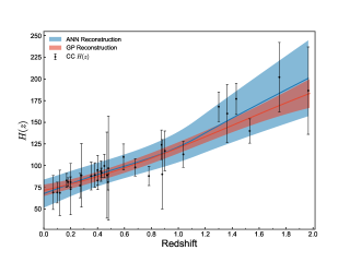
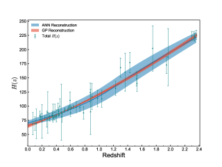
Figure 1: Left: The reconstructions of $H(z)$ from CC $H(z)$ data by using GP (red region) and ANN (blue region). The shaded region and the solid line denote the 1$\sigma$ confidence level errors and the best-fit values of reconstruction, respectively. The black points with error bars represent the observed CC $H(z)$ data. Right: Same as the left panel but for the Total $H(z)$ data.

II.3 Reconstruction method: Gaussian process

There is an integral between the Hubble parameter and the luminosity distance. In order to calibrate the distance using the $H(z)$ data, it is necessary to reconstruct a smooth curve of $H(z)$ with a non-parametric reconstruction technique firstly. Here, we briefly introduce the GP method that allows us to reconstruct a function from data straightforwardly without any parametric assumption. We adopt the GaPP Python code widely used in cosmology to implement the GP method (Seikel et al., 2012a, b; Zhang and Li, 2018; Cai et al., 2020; Wang et al., 2021; Seikel and Clarkson, 2013; Benisty et al., 2023; Briffa et al., 2020; Bernardo et al., 2022; Escamilla-Rivera et al., 2021). In this process, it is assumed that the value of the reconstructed function $f(z)$ evaluated at two different points $z$ and $\tilde{z}$ are connected by a covariance function $k(z,\tilde{z})$, and it only depends on two hyperparameters $\sigma_{f}$ and $\ell$. Although there are various and effective forms of the covariance function, according to the analysis in Seikel & Clarkson Seikel and Clarkson (2013), the squared exponential form with the Matérn $(\nu=9/2)$ covariance function can lead to more reliable results than all others. So we take it here, and its expression is

$$k(z,\tilde{z}) = \sigma_{f}^{2}\exp(-\frac{3|z-\tilde{z}|}{\ell})$$ (6)

$$\times (1+\frac{3|z-\tilde{z}|}{\ell}+\frac{27(z-\tilde{z})^{2}}{7\ell^{2}}$$

$$+ \frac{18|z-\tilde{z}|^{3}}{7\ell^{3}}+\frac{27(z-\tilde{z})^{4}}{35\ell^{4}}).$$

Here, the hyperparameter $\ell$ represents the characteristic length scale, indicating the distance over which significant changes occur in the function $f(z)$. The hyperparameter $\sigma_{f}$ represents the typical change or variation in the observed data. The values of two hyperparameters are optimized by the GP itself via the observational data. It is important to note that the optimization of these two hyperparameters is performed independently of the fitting process for the cosmological parameters. The reconstructed functions of $H(z)$ for the two cases, CC $H(z)$ and Total $H(z)$, are shown in Fig. 1.

II.4 Reconstruction method: artificial neural network

Here, we use the ANN method based on REFANN (Wang et al., 2020a) Python code to reconstruct a function of $H(z)$ from data, which also has been widely used in cosmology (Dialektopoulos et al., 2022; Benisty et al., 2023). The ANN method, completely driven by data, allows us to reconstruct a function from any kind of data without assuming a parametrization of the function. The optimal ANN model of reconstructing functions we used is the same as that selected by Wang et al. (Wang et al., 2020a), which has one hidden layer with 4096 neurons total. The reconstructed functions of $H(z)$ from the ANN are also shown in Fig. 1.

We can see that the confidence region reconstructed from the ANN is larger than that reconstructed from the GP method, which may be due to the basic logic and nature of these two techniques. One potential explanation for the observed discrepancy is the variance in the underlying assumptions and modeling approaches of GP and ANN. The GP method focuses on reconstructing a smooth function based on the covariance between data points, prioritizing the overall structure and correlations in the data. On the other hand, ANN approximates the underlying function using interconnected artificial neurons, allowing it to capture complex non-linear relationships. These inherent differences in modeling techniques can lead to variations in how the methods handle noise, outliers, and subtle features in the data, resulting in divergent reconstructions for $H(z)$. Additionally, the training and optimization processes employed by GP and ANN can contribute to the observed discrepancy. The selection of hyperparameters, such as the kernel function in GP or the network architecture in ANN, can significantly impact the models’ flexibility and generalization capabilities. Variations in the hyperparameter selection and training strategies may introduce sensitivities and biases that influence the inferred values of $H(z)$. Furthermore, it is important to acknowledge that GP and ANN have distinct strengths and limitations. GP excels at capturing uncertainties and estimating smooth functions, while ANN is effective in modeling complex non-linear relationships. These inherent differences in methodology can contribute to the observed discrepancies in the reconstructed values of $H(z)$.

In addition, the reconstructed values of Hubble constant ($H(z=0)$) by these two methods are also different, which is sensitive to the constraint on $\Omega_{k}$ as we will see later.

II.5 Methodology for estimation of $\Omega_{k}$

In the framework of the FLRW metric, the comoving distance $D_{C}(z)$ is defined as

$$D_{C}(z)=c\int_{0}^{z}\frac{dz^{\prime}}{H\left(z^{\prime}\right)},$$ (7)

where $c$ is the speed of light. With a reconstructed smooth function of $H(z)$, a smooth function of $D_{C}(z)$ could be calculated by integrating the function $H(z)$, and its confidence region also could be obtained by integrating the error of $H(z)$. Furthermore, the luminosity distance $D_{L}$ could be obtained by $D_{C}$ via

$$\frac{D_{L}}{(1+z)}=\begin{cases}\frac{c}{H_{0}}\frac{1}{\sqrt{\Omega_{k}}}\sinh\left[\sqrt{\Omega_{k}}D_{C}\frac{H_{0}}{c}\right]&\Omega_{k}>0,\\ D_{C}&\Omega_{k}=0,\\ \frac{c}{H_{0}}\frac{1}{\sqrt{\left|\Omega_{K}\right|}}\sin\left[\sqrt{\mid\Omega_{k}}\mid D_{C}\frac{H_{0}}{c}\right]&\Omega_{k}<0.\end{cases}$$ (8)

Note that in this calculation, the value of $H_{0}$ is adopted from the reconstructed value of $H(z=0)$. The uncertainty of $D_{L}$ could be obtained by

$$\sigma_{D_{L}}=\begin{cases}(1+z)\cosh\left[\sqrt{\left|\Omega_{k}\right|}D_{C}\frac{H_{0}}{c}\right]\sigma_{D_{C}}&\text{for}\quad\Omega_{k}>0,\\ (1+z)\sigma_{D_{C}}&\text{for}\quad\Omega_{k}=0,\\ (1+z)\cos\left[\sqrt{\left|\Omega_{k}\right|}D_{C}\frac{H_{0}}{c}\right]\sigma_{D_{C}}&\text{for}\quad\Omega_{k}<0.\end{cases}$$ (9)

The distance modulus reconstructed from $H(z)$ data $\mu_{H}$ can be further obtained by Eq. (2). Finally, the cosmic curvature parameter $\Omega_{k}$ could be estimated by minimizing the $\chi^{2}$ function of Eq. (3). Here, the uncertainty of reconstructed distance modulus $\sigma_{\mu_{H}}$ should be added to the covariance matrix as a systematic error via

$$(\mathbf{C}_{\text{stat}})_{ii}=(\mathbf{C}_{\text{stat}}^{\text{SN}})_{ii}+\sigma_{\mu_{H},i}^{2}.$$ (10)

We constrain the cosmological parameters using the emcee Python module based on the Markov Chain Monte Carlo analysis (Foreman-Mackey et al., 2013). There are two free parameters, $\Omega_{k}$ and the SNe Ia absolute magnitude $M_{B}$.

III Results and discussions

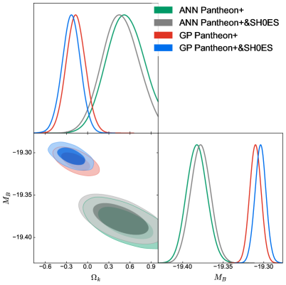
Figure 2: The constraints with the 1$\sigma$ and 2$\sigma$ confidence level on the cosmic curvature $\Omega_{k}$ and the SNe Ia absolute magnitude $M_{B}$ from two types of SNe Ia data set (Pantheon+ and Pantheon+&SH0ES) and with two reconstruction methods (GP and ANN), respectively, in the case of CC $H(z)$ data.

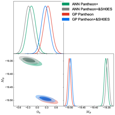
Figure 3: Same as Fig. 2, but for Total $H(z)$ data.

Table 3: The constraint results of $\Omega_{k}$ and $M_{B}$ with 1$\sigma$ confidence level for various data sets and reconstruction methods.

$H(z)$ data type	Parameters	GP Pantheon+	GP Pantheon+&SH0ES	ANN Pantheon+	ANN Pantheon+&SH0ES
CC $H(z)$	$\Omega_{k}$	$-0.17\pm 0.13$	$-0.23\pm 0.13$	$0.51^{+0.27}_{-0.24}$	$0.46\pm 0.25$
	$M_{B}$	$-19.310\pm 0.007$	$-19.304\pm 0.007$	$-19.382\pm 0.013$	$-19.378\pm 0.012$
Total $H(z)$	$\Omega_{k}$	$0.34\pm 0.13$	$0.26\pm 0.13$	$-0.18\pm 0.13$	$-0.27\pm 0.13$
	$M_{B}$	$-19.500\pm 0.006$	$-19.494\pm 0.005$	$-19.353\pm 0.006$	$-19.3465\pm 0.006$

Here, we combine two types of $H(z)$ data, two types of SNe Ia data, and two reconstruction methods to make a thorough investigation of the cosmic curvature. All the constraint contours of $\Omega_{k}$ and $M_{B}$ are shown in Figs. 2–3 and the best-fit values with 1 $\sigma$ confidence level are listed in Table 3.

In Fig. 2, we present the constraints on $\Omega_{k}$ and $M_{B}$ obtained from the CC $H(z)$ data in different scenarios. It is evident that there are differences between the contours derived from the two reconstruction methods. Specifically, concerning the GP method, the values of $M_{B}$ constrained from both the Pantheon+ and Pantheon+&SH0ES data sets are almost identical, which means the addition of SH0ES data is not helpful to the constraint on $M_{B}$. As for $\Omega_{k}$, the estimations from Pantheon+ and Pantheon+&SH0ES both favor a closed universe, while remaining consistent with a flat universe at the 2$\sigma$ confidence level. Moreover, we find an intriguing finding that the inclusion of SH0ES data does not appear to significantly impact the precision of the $\Omega_{k}$ constraint.

Regarding the ANN method, we find that the uncertainties of the two parameters (i.e., $\Omega_{k}$ and $M_{B}$) obtained from this approach are larger than those derived from the GP method. This discrepancy can be traced back to the left panel of Fig. 1, where we notice that the confidence region of $H(z)$ reconstructed by the ANN is notably broader compared to that reconstructed using the GP method. Additionally, as mentioned previously, the reconstructed values of the Hubble constant ($H(z=0)$) from these two methods are also different, which subsequently influences the constraint on $M_{B}$ as evident from the distinct contours observed in Fig. 2 for the GP and ANN methods. Concerning the estimation of $\Omega_{k}$, we find that not only do the uncertainties become larger when compared to the results obtained from the GP method, but the best-fit values also tend to favor an open universe, while remaining consistent with a flat universe within the 2$\sigma$ confidence level. Additionally, the addition of SH0ES data does not appear to significantly affect the constraint precision of $\Omega_{k}$ in the context of the ANN method.

Now, let’s focus on the Total $H(z)$ data, which has a sample size nearly twice as large as the CC $H(z)$ data. In Fig. 3, we present the 1D and 2D marginalized probability distributions of $\Omega_{k}$ and $M_{B}$ obtained from this dataset.

For the GP method, regarding the constraints on $\Omega_{k}$, we find a shift in the best-fit values compared with CC $H(z)$ data, now leaning towards a positive value, indicating support for an open universe, but the estimate from Pantheon+&SH0ES is still consistent with a flat universe at 2$\sigma$ confidence level. This change demonstrates that the addition of the BAO $H(z)$ observational data influences the estimation of $\Omega_{k}$ using this approach. Despite the Total $H(z)$ data having nearly twice the sample size of the CC $H(z)$ data, we find that the constraint precision of $\Omega_{k}$ is not notably improved compared to that derived from the CC $H(z)$ data.

In the case of the ANN reconstruction method, we find a substantial improvement in the constraints on both $\Omega_{k}$ and $M_{B}$ when using the Total $H(z)$ data compared to the results obtained from the CC $H(z)$ data. The constraints on $\Omega_{k}$ and $M_{B}$ have improved by approximately twice, indicating that the ANN method is more sensitive to the addition of the BAO $H(z)$ data. This sensitivity allows for better constraints on the cosmological parameters when incorporating the larger sample size provided by the Total $H(z)$ data. Regarding $\Omega_{k}$, both of the best-fit values from the two SNe Ia data sets favor a closed universe, while remaining consistent with a flat universe within the 2$\sigma$ confidence level.

IV Conclusion

Currently, the measurement inconsistencies between the early and late universe, such as the tensions in the Hubble constant, the $S_{8}$ parameter, and the cosmic curvature parameter, have raised questions about the validity of the standard cosmological model, i.e. the $\Lambda$CDM model. In this paper, we highlight the importance of determining the cosmic curvature parameter $\Omega_{k}$ and aim to make a thorough investigation for the model-independent measurement of $\Omega_{k}$ in the late universe with the observational data and statistical tools available to us. Therefore, we consider two types of $H(z)$ data sets (CC $H(z)$ data and Total data), two types of SNe Ia data sets (Pantheon+ and Pantheon+&SH0ES), and two reconstruction methods (GP method and ANN method).

The GP method has yielded the most precise constraint on $\Omega_{k}$, with a constraint precision of $\xi(\Omega_{k})=0.13$ for any combination of data, surpassing the recent measurements of $\Omega_{k}$ using similar methods (Dhawan et al., 2021; Wei and Wu, 2017; Yu and Wang, 2016; Wang et al., 2021). Overall, the estimations obtained through the GP method consistently support a flat universe at the 2$\sigma$ confidence level.

It is worth noting that the estimation of $\Omega_{k}$ in this study is influenced by the choice of reconstruction method. The ANN reconstruction method exhibits higher sensitivity to the addition of $H(z)$ data. By combining the BAO $H(z)$ data, the constraint precision based on the ANN method becomes comparable to that obtained using the GP method. However, a discrepancy exists between the best-fit values obtained by these two reconstruction methods, indicating a dependence on the reconstruction approach. As a consequence, the method employed in this study to evaluate $\Omega_{k}$ may be less robust due to its sensitivity to the reconstruction method. Nevertheless, we expect that with the improvement of sample size and precision of observational $H(z)$ data, the estimation of $\Omega_{k}$ using this approach will become more robust and reliable.

References

- Riess et al. (1998) Adam G. Riess et al. (Supernova Search Team), “Observational evidence from supernovae for an accelerating universe and a cosmological constant,” Astron. J. 116, 1009–1038 (1998), arXiv:astro-ph/9805201 .
- Perlmutter et al. (1999) S. Perlmutter et al. (Supernova Cosmology Project), “Measurements of and from 42 high redshift supernovae,” Astrophys. J. 517, 565–586 (1999), arXiv:astro-ph/9812133 .
- Spergel et al. (2003) D. N. Spergel et al. (WMAP), “First year Wilkinson Microwave Anisotropy Probe (WMAP) observations: Determination of cosmological parameters,” Astrophys. J. Suppl. 148, 175–194 (2003), arXiv:astro-ph/0302209 .
- Tegmark et al. (2004) Max Tegmark et al. (SDSS), “Cosmological parameters from SDSS and WMAP,” Phys. Rev. D 69, 103501 (2004), arXiv:astro-ph/0310723 .
- Abazajian et al. (2004) Kevork Abazajian et al. (SDSS), “The Second data release of the Sloan digital sky survey,” Astron. J. 128, 502–512 (2004), arXiv:astro-ph/0403325 .
- Ade et al. (2016) P. A. R. Ade et al. (Planck), “Planck 2015 results. XIII. Cosmological parameters,” Astron. Astrophys. 594, A13 (2016), arXiv:1502.01589 [astro-ph.CO] .
- Aghanim et al. (2020) N. Aghanim et al. (Planck), “Planck 2018 results. VI. Cosmological parameters,” Astron. Astrophys. 641, A6 (2020), [Erratum: Astron.Astrophys. 652, C4 (2021)], arXiv:1807.06209 [astro-ph.CO] .
- Riess et al. (2019) Adam G. Riess, Stefano Casertano, Wenlong Yuan, Lucas M. Macri, and Dan Scolnic, “Large Magellanic Cloud Cepheid Standards Provide a 1% Foundation for the Determination of the Hubble Constant and Stronger Evidence for Physics beyond CDM,” Astrophys. J. 876, 85 (2019), arXiv:1903.07603 [astro-ph.CO] .
- Qi et al. (2021) Jing-Zhao Qi, Jia-Wei Zhao, Shuo Cao, Marek Biesiada, and Yuting Liu, “Measurements of the Hubble constant and cosmic curvature with quasars: ultracompact radio structure and strong gravitational lensing,” Mon. Not. Roy. Astron. Soc. 503, 2179–2186 (2021), arXiv:2011.00713 [astro-ph.CO] .
- Qi et al. (2022) Jing-Zhao Qi, Yu Cui, Wei-Hong Hu, Jing-Fei Zhang, Jing-Lei Cui, and Xin Zhang, “Strongly lensed type Ia supernovae as a precise late-Universe probe of measuring the Hubble constant and cosmic curvature,” Phys. Rev. D 106, 023520 (2022), arXiv:2202.01396 [astro-ph.CO] .
- Cao et al. (2022) Meng-Di Cao, Jie Zheng, Jing-Zhao Qi, Xin Zhang, and Zong-Hong Zhu, “A New Way to Explore Cosmological Tensions Using Gravitational Waves and Strong Gravitational Lensing,” Astrophys. J. 934, 108 (2022), arXiv:2112.14564 [astro-ph.CO] .
- Di Valentino et al. (2019) Eleonora Di Valentino, Alessandro Melchiorri, and Joseph Silk, “Planck evidence for a closed Universe and a possible crisis for cosmology,” Nature Astron. 4, 196–203 (2019), arXiv:1911.02087 [astro-ph.CO] .
- Di Valentino et al. (2021a) Eleonora Di Valentino, Alessandro Melchiorri, and Joseph Silk, “Investigating Cosmic Discordance,” Astrophys. J. Lett. 908, L9 (2021a), arXiv:2003.04935 [astro-ph.CO] .
- Handley (2021) Will Handley, “Curvature tension: evidence for a closed universe,” Phys. Rev. D 103, L041301 (2021), arXiv:1908.09139 [astro-ph.CO] .
- Riess et al. (2021) Adam G. Riess, Stefano Casertano, Wenlong Yuan, J. Bradley Bowers, Lucas Macri, Joel C. Zinn, and Dan Scolnic, “Cosmic Distances Calibrated to 1% Precision with Gaia EDR3 Parallaxes and Hubble Space Telescope Photometry of 75 Milky Way Cepheids Confirm Tension with CDM,” Astrophys. J. Lett. 908, L6 (2021), arXiv:2012.08534 [astro-ph.CO] .
- Di Valentino et al. (2021b) Eleonora Di Valentino, Olga Mena, Supriya Pan, Luca Visinelli, Weiqiang Yang, Alessandro Melchiorri, David F. Mota, Adam G. Riess, and Joseph Silk, “In the realm of the Hubble tension—a review of solutions,” Class. Quant. Grav. 38, 153001 (2021b), arXiv:2103.01183 [astro-ph.CO] .
- Vagnozzi (2020) Sunny Vagnozzi, “New physics in light of the tension: An alternative view,” Phys. Rev. D 102, 023518 (2020), arXiv:1907.07569 [astro-ph.CO] .
- Zhang (2019) Xin Zhang, “Gravitational wave standard sirens and cosmological parameter measurement,” Sci. China Phys. Mech. Astron. 62, 110431 (2019), arXiv:1905.11122 [astro-ph.CO] .
- Xu and Zhang (2020) YiDong Xu and Xin Zhang, “Cosmological parameter measurement and neutral hydrogen 21 cm sky survey with the Square Kilometre Array,” Sci. China Phys. Mech. Astron. 63, 270431 (2020), arXiv:2002.00572 [astro-ph.CO] .
- Li et al. (2013) Miao Li, Xiao-Dong Li, Yin-Zhe Ma, Xin Zhang, and Zhenhui Zhang, “Planck Constraints on Holographic Dark Energy,” JCAP 09, 021 (2013), arXiv:1305.5302 [astro-ph.CO] .
- Qi and Zhang (2020) Jing-Zhao Qi and Xin Zhang, “A new cosmological probe using super-massive black hole shadows,” Chin. Phys. C 44, 055101 (2020), arXiv:1906.10825 [astro-ph.CO] .
- Vattis et al. (2019) Kyriakos Vattis, Savvas M. Koushiappas, and Abraham Loeb, “Dark matter decaying in the late Universe can relieve the H0 tension,” Phys. Rev. D 99, 121302 (2019), arXiv:1903.06220 [astro-ph.CO] .
- Zhang et al. (2014a) Jing-Fei Zhang, Jia-Jia Geng, and Xin Zhang, “Neutrinos and dark energy after Planck and BICEP2: data consistency tests and cosmological parameter constraints,” JCAP 10, 044 (2014a), arXiv:1408.0481 [astro-ph.CO] .
- Guo et al. (2019) Rui-Yun Guo, Jing-Fei Zhang, and Xin Zhang, “Can the tension be resolved in extensions to CDM cosmology?” JCAP 02, 054 (2019), arXiv:1809.02340 [astro-ph.CO] .
- Zhao et al. (2017) Ming-Ming Zhao, Dong-Ze He, Jing-Fei Zhang, and Xin Zhang, “Search for sterile neutrinos in holographic dark energy cosmology: Reconciling Planck observation with the local measurement of the Hubble constant,” Phys. Rev. D 96, 043520 (2017), arXiv:1703.08456 [astro-ph.CO] .
- Guo and Zhang (2017) Rui-Yun Guo and Xin Zhang, “Constraints on inflation revisited: An analysis including the latest local measurement of the Hubble constant,” Eur. Phys. J. C 77, 882 (2017), arXiv:1704.04784 [astro-ph.CO] .
- Gao et al. (2021) Li-Yang Gao, Ze-Wei Zhao, She-Sheng Xue, and Xin Zhang, “Relieving the H 0 tension with a new interacting dark energy model,” JCAP 07, 005 (2021), arXiv:2101.10714 [astro-ph.CO] .
- Gao et al. (2022) Li-Yang Gao, She-Sheng Xue, and Xin Zhang, “Dark energy and matter interacting scenario can relieve and tensions,” (2022), arXiv:2212.13146 [astro-ph.CO] .
- Heymans et al. (2021) Catherine Heymans et al., “KiDS-1000 Cosmology: Multi-probe weak gravitational lensing and spectroscopic galaxy clustering constraints,” Astron. Astrophys. 646, A140 (2021), arXiv:2007.15632 [astro-ph.CO] .
- Stevens et al. (2023) Jordan Stevens, Hasti Khoraminezhad, and Shun Saito, “Constraining the spatial curvature with cosmic expansion history in a cosmological model with a non-standard sound horizon,” JCAP 07, 046 (2023), arXiv:2212.09804 [astro-ph.CO] .
- Efstathiou and Gratton (2020) George Efstathiou and Steven Gratton, “The evidence for a spatially flat Universe,” Mon. Not. Roy. Astron. Soc. 496, L91–L95 (2020), arXiv:2002.06892 [astro-ph.CO] .
- Vagnozzi et al. (2021a) Sunny Vagnozzi, Eleonora Di Valentino, Stefano Gariazzo, Alessandro Melchiorri, Olga Mena, and Joseph Silk, “The galaxy power spectrum take on spatial curvature and cosmic concordance,” Phys. Dark Univ. 33, 100851 (2021a), arXiv:2010.02230 [astro-ph.CO] .
- Vagnozzi et al. (2021b) Sunny Vagnozzi, Abraham Loeb, and Michele Moresco, “Eppur è piatto? The Cosmic Chronometers Take on Spatial Curvature and Cosmic Concordance,” Astrophys. J. 908, 84 (2021b), arXiv:2011.11645 [astro-ph.CO] .
- Gonzalez et al. (2021) Javier E. Gonzalez, Micol Benetti, Rodrigo von Marttens, and Jailson Alcaniz, “Testing the consistency between cosmological data: the impact of spatial curvature and the dark energy EoS,” JCAP 11, 060 (2021), arXiv:2104.13455 [astro-ph.CO] .
- Zuckerman and Anchordoqui (2022) Ella Zuckerman and Luis A. Anchordoqui, “Spatial curvature sensitivity to local H0 from the Cepheid distance ladder,” JHEAp 33, 10–13 (2022), arXiv:2110.05346 [astro-ph.CO] .
- Akarsu et al. (2023) Ozgur Akarsu, Eleonora Di Valentino, Suresh Kumar, Maya Ozyigit, and Shivani Sharma, “Testing spatial curvature and anisotropic expansion on top of the CDM model,” Phys. Dark Univ. 39, 101162 (2023), arXiv:2112.07807 [astro-ph.CO] .
- Glanville et al. (2022) Aaron Glanville, Cullan Howlett, and Tamara M. Davis, “Full-shape galaxy power spectra and the curvature tension,” Mon. Not. Roy. Astron. Soc. 517, 3087–3100 (2022), arXiv:2205.05892 [astro-ph.CO] .
- Bel et al. (2022) Julien Bel, Julien Larena, Roy Maartens, Christian Marinoni, and Louis Perenon, “Constraining spatial curvature with large-scale structure,” JCAP 09, 076 (2022), arXiv:2206.03059 [astro-ph.CO] .
- Favale et al. (2023) Arianna Favale, Adrià Gómez-Valent, and Marina Migliaccio, “Cosmic chronometers to calibrate the ladders and measure the curvature of the Universe. A model-independent study,” Mon. Not. Roy. Astron. Soc. 523, 3406–3422 (2023), arXiv:2301.09591 [astro-ph.CO] .
- Cao et al. (2021) Shulei Cao, Joseph Ryan, and Bharat Ratra, “Using Pantheon and DES supernova, baryon acoustic oscillation, and Hubble parameter data to constrain the Hubble constant, dark energy dynamics, and spatial curvature,” Mon. Not. Roy. Astron. Soc. 504, 300–310 (2021), arXiv:2101.08817 [astro-ph.CO] .
- Zhai et al. (2020) Zhongxu Zhai, Chan-Gyung Park, Yun Wang, and Bharat Ratra, “CMB distance priors revisited: effects of dark energy dynamics, spatial curvature, primordial power spectrum, and neutrino parameters,” JCAP 07, 009 (2020), arXiv:1912.04921 [astro-ph.CO] .
- Ryan et al. (2019) Joseph Ryan, Yun Chen, and Bharat Ratra, “Baryon acoustic oscillation, Hubble parameter, and angular size measurement constraints on the Hubble constant, dark energy dynamics, and spatial curvature,” Mon. Not. Roy. Astron. Soc. 488, 3844–3856 (2019), arXiv:1902.03196 [astro-ph.CO] .
- Park and Ratra (2019) Chan-Gyung Park and Bharat Ratra, “Measuring the Hubble constant and spatial curvature from supernova apparent magnitude, baryon acoustic oscillation, and Hubble parameter data,” Astrophys. Space Sci. 364, 134 (2019), arXiv:1809.03598 [astro-ph.CO] .
- Penton et al. (2018) Jarred Penton, Jacob Peyton, Aasim Zahoor, and Bharat Ratra, “Median Statistics Analysis of Deuterium Abundance Measurements and Spatial Curvature Constraints,” Publ. Astron. Soc. Pac. 130, 114001 (2018), arXiv:1808.01490 [astro-ph.CO] .
- Ryan et al. (2018) Joseph Ryan, Sanket Doshi, and Bharat Ratra, “Constraints on dark energy dynamics and spatial curvature from Hubble parameter and baryon acoustic oscillation data,” Mon. Not. Roy. Astron. Soc. 480, 759–767 (2018), arXiv:1805.06408 [astro-ph.CO] .
- Yu et al. (2018) Hai Yu, Bharat Ratra, and Fa-Yin Wang, “Hubble Parameter and Baryon Acoustic Oscillation Measurement Constraints on the Hubble Constant, the Deviation from the Spatially Flat CDM Model, the Deceleration–Acceleration Transition Redshift, and Spatial Curvature,” Astrophys. J. 856, 3 (2018), arXiv:1711.03437 [astro-ph.CO] .
- Collett et al. (2019) Thomas Collett, Francesco Montanari, and Syksy Rasanen, “Model-Independent Determination of and from Strong Lensing and Type Ia Supernovae,” Phys. Rev. Lett. 123, 231101 (2019), arXiv:1905.09781 [astro-ph.CO] .
- Wang et al. (2021) Guo-Jian Wang, Xiao-Jiao Ma, and Jun-Qing Xia, “Machine learning the cosmic curvature in a model-independent way,” Mon. Not. Roy. Astron. Soc. 501, 5714–5722 (2021), arXiv:2004.13913 [astro-ph.CO] .
- Wang et al. (2020a) Guo-Jian Wang, Xiao-Jiao Ma, Si-Yao Li, and Jun-Qing Xia, “Reconstructing Functions and Estimating Parameters with Artificial Neural Networks: A Test with a Hubble Parameter and SNe Ia,” Astrophys. J. Suppl. 246, 13 (2020a), arXiv:1910.03636 [astro-ph.CO] .
- Clarkson et al. (2007) Chris Clarkson, Marina Cortes, and Bruce A. Bassett, “Dynamical Dark Energy or Simply Cosmic Curvature?” JCAP 08, 011 (2007), arXiv:astro-ph/0702670 .
- Clarkson et al. (2008) Chris Clarkson, Bruce Bassett, and Teresa Hui-Ching Lu, “A general test of the Copernican Principle,” Phys. Rev. Lett. 101, 011301 (2008), arXiv:0712.3457 [astro-ph] .
- Wang et al. (2020b) Bo Wang, Jing-Zhao Qi, Jing-Fei Zhang, and Xin Zhang, “Cosmological Model-independent Constraints on Spatial Curvature from Strong Gravitational Lensing and SN Ia Observations,” Astrophys. J. 898, 100 (2020b), arXiv:1910.12173 [astro-ph.CO] .
- Xia et al. (2017) Jun-Qing Xia, Hai Yu, Guo-Jian Wang, Shu-Xun Tian, Zheng-Xiang Li, Shuo Cao, and Zong-Hong Zhu, “Revisiting Studies of the Statistical Property of a Strong Gravitational Lens System and Model-independent Constraint on the Curvature of the Universe,” Astrophys. J. 834, 75 (2017), arXiv:1611.04731 [astro-ph.CO] .
- Cai et al. (2016) Rong-Gen Cai, Zong-Kuan Guo, and Tao Yang, “Null test of the cosmic curvature using and supernovae data,” Phys. Rev. D 93, 043517 (2016), arXiv:1509.06283 [astro-ph.CO] .
- Räsänen et al. (2015) Syksy Räsänen, Krzysztof Bolejko, and Alexis Finoguenov, “New Test of the Friedmann-Lemaître-Robertson-Walker Metric Using the Distance Sum Rule,” Phys. Rev. Lett. 115, 101301 (2015), arXiv:1412.4976 [astro-ph.CO] .
- Wang et al. (2022) Yan-Jin Wang, Jing-Zhao Qi, Bo Wang, Jing-Fei Zhang, Jing-Lei Cui, and Xin Zhang, “Cosmological model-independent measurement of cosmic curvature using distance sum rule with the help of gravitational waves,” Mon. Not. Roy. Astron. Soc. 516, 5187–5195 (2022), arXiv:2201.12553 [astro-ph.CO] .
- Qi et al. (2019) Jing-Zhao Qi, Shuo Cao, Sixuan Zhang, Marek Biesiada, Yan Wu, and Zong-Hong Zhu, “The distance sum rule from strong lensing systems and quasars – test of cosmic curvature and beyond,” Mon. Not. Roy. Astron. Soc. 483, 1104–1113 (2019), arXiv:1803.01990 [astro-ph.CO] .
- Wei and Wu (2017) Jun-Jie Wei and Xue-Feng Wu, “An Improved Method to Measure the Cosmic Curvature,” Astrophys. J. 838, 160 (2017), arXiv:1611.00904 [astro-ph.CO] .
- Yu and Wang (2016) H. Yu and F. Y. Wang, “New model-independent method to test the curvature of the universe,” Astrophys. J. 828, 85 (2016), arXiv:1605.02483 [astro-ph.CO] .
- Dhawan et al. (2021) Suhail Dhawan, Justin Alsing, and Sunny Vagnozzi, “Non-parametric spatial curvature inference using late-Universe cosmological probes,” Mon. Not. Roy. Astron. Soc. 506, L1–L5 (2021), arXiv:2104.02485 [astro-ph.CO] .
- Brout et al. (2022) Dillon Brout et al., “The Pantheon+ Analysis: Cosmological Constraints,” Astrophys. J. 938, 110 (2022), arXiv:2202.04077 [astro-ph.CO] .
- Scolnic et al. (2018) D. M. Scolnic et al. (Pan-STARRS1), “The Complete Light-curve Sample of Spectroscopically Confirmed SNe Ia from Pan-STARRS1 and Cosmological Constraints from the Combined Pantheon Sample,” Astrophys. J. 859, 101 (2018), arXiv:1710.00845 [astro-ph.CO] .
- Zhang et al. (2014b) Cong Zhang, Han Zhang, Shuo Yuan, Tong-Jie Zhang, and Yan-Chun Sun, “Four new observational data from luminous red galaxies in the Sloan Digital Sky Survey data release seven,” Res. Astron. Astrophys. 14, 1221–1233 (2014b), arXiv:1207.4541 [astro-ph.CO] .
- Stern et al. (2010) Daniel Stern, Raul Jimenez, Licia Verde, Marc Kamionkowski, and S. Adam Stanford, “Cosmic Chronometers: Constraining the Equation of State of Dark Energy. I: H(z) Measurements,” JCAP 02, 008 (2010), arXiv:0907.3149 [astro-ph.CO] .
- Moresco et al. (2012) M. Moresco et al., “Improved constraints on the expansion rate of the Universe up to z~1.1 from the spectroscopic evolution of cosmic chronometers,” JCAP 08, 006 (2012), arXiv:1201.3609 [astro-ph.CO] .
- Moresco et al. (2016) Michele Moresco, Lucia Pozzetti, Andrea Cimatti, Raul Jimenez, Claudia Maraston, Licia Verde, Daniel Thomas, Annalisa Citro, Rita Tojeiro, and David Wilkinson, “A 6% measurement of the Hubble parameter at : direct evidence of the epoch of cosmic re-acceleration,” JCAP 05, 014 (2016), arXiv:1601.01701 [astro-ph.CO] .
- Ratsimbazafy et al. (2017) A. L. Ratsimbazafy, S. I. Loubser, S. M. Crawford, C. M. Cress, B. A. Bassett, R. C. Nichol, and P. Väisänen, “Age-dating Luminous Red Galaxies observed with the Southern African Large Telescope,” Mon. Not. Roy. Astron. Soc. 467, 3239–3254 (2017), arXiv:1702.00418 [astro-ph.CO] .
- Moresco (2015) Michele Moresco, “Raising the bar: new constraints on the Hubble parameter with cosmic chronometers at z 2,” Mon. Not. Roy. Astron. Soc. 450, L16–L20 (2015), arXiv:1503.01116 [astro-ph.CO] .
- Gaztanaga et al. (2009) Enrique Gaztanaga, Anna Cabre, and Lam Hui, “Clustering of Luminous Red Galaxies IV: Baryon Acoustic Peak in the Line-of-Sight Direction and a Direct Measurement of H(z),” Mon. Not. Roy. Astron. Soc. 399, 1663–1680 (2009), arXiv:0807.3551 [astro-ph] .
- Oka et al. (2014) Akira Oka, Shun Saito, Takahiro Nishimichi, Atsushi Taruya, and Kazuhiro Yamamoto, “Simultaneous constraints on the growth of structure and cosmic expansion from the multipole power spectra of the SDSS DR7 LRG sample,” Mon. Not. Roy. Astron. Soc. 439, 2515–2530 (2014), arXiv:1310.2820 [astro-ph.CO] .
- Wang et al. (2017) Yuting Wang et al. (BOSS), “The clustering of galaxies in the completed SDSS-III Baryon Oscillation Spectroscopic Survey: tomographic BAO analysis of DR12 combined sample in configuration space,” Mon. Not. Roy. Astron. Soc. 469, 3762–3774 (2017), arXiv:1607.03154 [astro-ph.CO] .
- Chuang and Wang (2013) Chia-Hsun Chuang and Yun Wang, “Modeling the Anisotropic Two-Point Galaxy Correlation Function on Small Scales and Improved Measurements of , , and from the Sloan Digital Sky Survey DR7 Luminous Red Galaxies,” Mon. Not. Roy. Astron. Soc. 435, 255–262 (2013), arXiv:1209.0210 [astro-ph.CO] .
- Alam et al. (2017) Shadab Alam et al. (BOSS), “The clustering of galaxies in the completed SDSS-III Baryon Oscillation Spectroscopic Survey: cosmological analysis of the DR12 galaxy sample,” Mon. Not. Roy. Astron. Soc. 470, 2617–2652 (2017), arXiv:1607.03155 [astro-ph.CO] .
- Anderson et al. (2014) Lauren Anderson et al. (BOSS), “The clustering of galaxies in the SDSS-III Baryon Oscillation Spectroscopic Survey: baryon acoustic oscillations in the Data Releases 10 and 11 Galaxy samples,” Mon. Not. Roy. Astron. Soc. 441, 24–62 (2014), arXiv:1312.4877 [astro-ph.CO] .
- Blake et al. (2012) Chris Blake et al., “The WiggleZ Dark Energy Survey: Joint measurements of the expansion and growth history at z 1,” Mon. Not. Roy. Astron. Soc. 425, 405–414 (2012), arXiv:1204.3674 [astro-ph.CO] .
- Zhao et al. (2019) Gong-Bo Zhao et al., “The clustering of the SDSS-IV extended Baryon Oscillation Spectroscopic Survey DR14 quasar sample: a tomographic measurement of cosmic structure growth and expansion rate based on optimal redshift weights,” Mon. Not. Roy. Astron. Soc. 482, 3497–3513 (2019), arXiv:1801.03043 [astro-ph.CO] .
- Busca et al. (2013) Nicolas G. Busca et al., “Baryon Acoustic Oscillations in the Ly- forest of BOSS quasars,” Astron. Astrophys. 552, A96 (2013), arXiv:1211.2616 [astro-ph.CO] .
- Bautista et al. (2017) Julian E. Bautista et al., “Measurement of baryon acoustic oscillation correlations at with SDSS DR12 Ly-Forests,” Astron. Astrophys. 603, A12 (2017), arXiv:1702.00176 [astro-ph.CO] .
- Delubac et al. (2015) Timothée Delubac et al. (BOSS), “Baryon acoustic oscillations in the Ly forest of BOSS DR11 quasars,” Astron. Astrophys. 574, A59 (2015), arXiv:1404.1801 [astro-ph.CO] .
- Font-Ribera et al. (2014) Andreu Font-Ribera et al. (BOSS), “Quasar-Lyman Forest Cross-Correlation from BOSS DR11 : Baryon Acoustic Oscillations,” JCAP 05, 027 (2014), arXiv:1311.1767 [astro-ph.CO] .
- Moresco et al. (2020) Michele Moresco, Raul Jimenez, Licia Verde, Andrea Cimatti, and Lucia Pozzetti, “Setting the Stage for Cosmic Chronometers. II. Impact of Stellar Population Synthesis Models Systematics and Full Covariance Matrix,” Astrophys. J. 898, 82 (2020), arXiv:2003.07362 [astro-ph.GA] .
- Seikel et al. (2012a) Marina Seikel, Chris Clarkson, and Mathew Smith, “Reconstruction of dark energy and expansion dynamics using Gaussian processes,” JCAP 06, 036 (2012a), arXiv:1204.2832 [astro-ph.CO] .
- Seikel et al. (2012b) Marina Seikel, Sahba Yahya, Roy Maartens, and Chris Clarkson, “Using H(z) data as a probe of the concordance model,” Phys. Rev. D 86, 083001 (2012b), arXiv:1205.3431 [astro-ph.CO] .
- Zhang and Li (2018) Ming-Jian Zhang and Hong Li, “Gaussian processes reconstruction of dark energy from observational data,” Eur. Phys. J. C 78, 460 (2018), arXiv:1806.02981 [astro-ph.CO] .
- Cai et al. (2020) Yi-Fu Cai, Martiros Khurshudyan, and Emmanuel N. Saridakis, “Model-independent reconstruction of gravity from Gaussian Processes,” Astrophys. J. 888, 62 (2020), arXiv:1907.10813 [astro-ph.CO] .
- Seikel and Clarkson (2013) Marina Seikel and Chris Clarkson, “Optimising Gaussian processes for reconstructing dark energy dynamics from supernovae,” preprint (arXiv:1311.6678) (2013), arXiv:1311.6678 [astro-ph.CO] .
- Benisty et al. (2023) David Benisty, Jurgen Mifsud, Jackson Levi Said, and Denitsa Staicova, “On the robustness of the constancy of the Supernova absolute magnitude: Non-parametric reconstruction & Bayesian approaches,” Phys. Dark Univ. 39, 101160 (2023), arXiv:2202.04677 [astro-ph.CO] .
- Briffa et al. (2020) Rebecca Briffa, Salvatore Capozziello, Jackson Levi Said, Jurgen Mifsud, and Emmanuel N. Saridakis, “Constraining teleparallel gravity through Gaussian processes,” Class. Quant. Grav. 38, 055007 (2020), arXiv:2009.14582 [gr-qc] .
- Bernardo et al. (2022) Reginald Christian Bernardo, Daniela Grandón, Jackson Said Levi, and Víctor H. Cárdenas, “Parametric and nonparametric methods hint dark energy evolution,” Phys. Dark Univ. 36, 101017 (2022), arXiv:2111.08289 [astro-ph.CO] .
- Escamilla-Rivera et al. (2021) Celia Escamilla-Rivera, Jackson Levi Said, and Jurgen Mifsud, “Performance of non-parametric reconstruction techniques in the late-time universe,” JCAP 10, 016 (2021), arXiv:2105.14332 [astro-ph.CO] .
- Dialektopoulos et al. (2022) Konstantinos Dialektopoulos, Jackson Levi Said, Jurgen Mifsud, Joseph Sultana, and Kristian Zarb Adami, “Neural network reconstruction of late-time cosmology and null tests,” JCAP 02, 023 (2022), arXiv:2111.11462 [astro-ph.CO] .
- Foreman-Mackey et al. (2013) Daniel Foreman-Mackey, David W. Hogg, Dustin Lang, and Jonathan Goodman, “emcee: The MCMC Hammer,” Publ. Astron. Soc. Pac. 125, 306–312 (2013), arXiv:1202.3665 [astro-ph.IM] .