Approximately Bayes-Optimal Pseudo Label Selection
Abstract
Semi-supervised learning by self-training heavily relies on pseudo-label selection (PLS). The selection often depends on the initial model fit on labeled data. Early overfitting might thus be propagated to the final model by selecting instances with overconfident but erroneous predictions, often referred to as confirmation bias. This paper introduces BPLS, a Bayesian framework for PLS that aims to mitigate this issue. At its core lies a criterion for selecting instances to label: an analytical approximation of the posterior predictive of pseudo-samples. We derive this selection criterion by proving Bayes optimality of the posterior predictive of pseudo-samples. We further overcome computational hurdles by approximating the criterion analytically. Its relation to the marginal likelihood allows us to come up with an approximation based on Laplace’s method and the Gaussian integral. We empirically assess BPLS for parametric generalized linear and non-parametric generalized additive models on simulated and real-world data. When faced with high-dimensional data prone to overfitting, BPLS outperforms traditional PLS methods.111Code available at: https://anonymous.4open.science/r/Bayesian-pls
1 INTRODUCTION
Labeled data are scarce in many learning settings. This can be due to a variety of reasons such as restrictions on time, knowledge, or financial resources. Unlabeled data, however, are often much more accessible. This has given rise to the paradigm of semi-supervised learning (SSL), where information from unlabeled data is integrated into model training to improve predictions in a supervised learning framework. Within SSL, an intuitive and widely used approach is referred to as self-training or pseudo-labeling [Shi et al., 2018, Lee et al., 2013, McClosky et al., 2006]. The idea is to fit an initial model to labeled data and iteratively assign pseudo-labels to unlabeled data according to the model’s predictions. The latter requires a criterion (sometimes called confidence measure) for pseudo-label selection (PLS), that is, the selection of instances to be pseudo-labeled and added to the training data.
By design, self-training strongly relies on the initial model fit and the way instances are selected to be pseudo-labeled. Everything hinges upon the interplay between the selection criterion and the initial model’s generalization performance. If the initial model generalizes poorly, initial misconceptions can propagate throughout the process, only making things worse. High-dimensional data prone to overfitting are particularly sensitive to such confirmation bias [Arazo et al., 2020]. Usually, self-training’s sweet spot lies somewhere else: When the labeled data allow the model to learn sufficiently well while still leaving some room for improvement. Generally, the poorer the initial generalization, the harder it is to select sensible pseudo-labels to improve generalization, i.e., the more crucial the role of the selection criterion. Note that SSL is applied to data with high shares (typically over [Sohn et al., 2020, Arazo et al., 2020]) of unlabeled data, where initial overfitting is likely for high-dimensional models, while final overfitting is not.
1.1 Motivation
Accordingly, we strive for a selection criterion that is robust with respect to the initial model fit, i.e., its learned parameters. At the same time, it should still exploit the information in the labeled data. Such a measure calls for disentangling the uncertainty contributions of the data and the model’s parameters. This is in line with recent work in uncertainty quantification (UQ) that suggests decomposing epistemic uncertainty into approximation uncertainty driven by (a lack of) data and modeling uncertainty driven by (primarily parametric) assumptions [Hüllermeier and Waegeman, 2021]. Bayesian inference offers a sound and consistent framework for this distinction. Its rationale of technically modeling not only data but also parameters as random variables has proven to offer much insight into UQ for machine learning [Hüllermeier and Waegeman, 2021] and deep learning [Abdar et al., 2021, Malinin and Gales, 2018].
We exploit the Bayesian framework for pinpointing uncertainty with regard to data and parameters in PLS. Our approach of Bayesian pseudo-label selection (BPLS) enables us to choose pseudo-labels that are likely given the observed labeled data but not necessarily likely given the estimated parameters of the fitted model. What is more, BPLS allows to include prior information not only for predicting but also for selecting pseudo-labels. Notably, BPLS is flexible enough to be applied to any kind of predictive model whose likelihood and Fisher-information are accessible, including non-Bayesian models. BPLS entails a Bayes optimal selection criterion, the pseudo posterior predictive (PPP). Its intuition is straightforward yet effective: By averaging over all parameter values, PPP is more robust towards the initial fit compared to the predictive distribution based on a single optimal parameter vector. Our approximate version of the PPP is simple and computationally cheap to evaluate: with being the likelihood and the Fisher-information matrix at the fitted parameter vector . As an approximation of the joint PPP, it does not require an i.i.d. assumption, rendering it applicable to a wide range of applied learning setups.
1.2 Main Contributions
(1) We derive PPP by formalizing PLS as a decision problem and show222Proofs of all theorems in this paper can be found in the supplementary material. that PPP corresponds to the Bayes criterion, rendering selecting instances with regard to it Bayes optimal, see sections 2.1 and 2.2.
(2) Since our selection criterion includes a possibly intractable integral, we provide analytical approximations, exploiting Laplace’s method and the Gaussian integral, both for uninformative and informative priors. Using varying levels of accuracy, we balance the trade-off between computational feasibility and precision, see Section 3.
(3) We provide empirical evidence333 Implementations of the proposed methods as well as reproducible scripts for the experiments are provided in the anonymous repository named Bayesian-pls (\sayBayesian, please!), see abstract. for BPLS’ superiority over traditionally predominant PLS methods in case of semi-supervised generalized additive models (GAMs) and generalized linear models (GLMs) faced with high-dimensional data prone to overfitting, see Section 4.
2 BAYESIAN PLS
Most semi-supervised methods deal with classification or clustering tasks [Van Engelen and Hoos, 2020, Chapelle et al., 2006]. Loosely leaning on [Triguero et al., 2015], we formalize SSL as follows. Consider labeled data
| (1) |
and unlabeled data
| (2) |
from the same data generation process, where is the feature space and is the categorical target space. The aim of SSL is to learn a predictive classification function such that utilizing both and . As is customary in self-training, we start by fitting a model with unknown parameter vector , compact with , on labeled data . Our goal is – as usual – to learn the conditional distribution of through from observing features , and responses in . Adopting the Bayesian perspective, we can state a prior function over as . The prior can represent information on but may also be uninformative.
Within existing frameworks for self-training (see Section 5) in SSL, one could deploy such a Bayesian setting for predicting unknown labels of as well as for the final predictions on unseen test data. However, we aim at a Bayesian framework for selecting pseudo-labels. This is beneficial for two reasons. First and foremost, considering the Bayesian posterior predictive distribution in PLS will turn out to be more robust towards the initial fit on than classical selection criteria. Second, the Bayesian engine brings along the usual benefit of allowing to explicitly account for prior knowledge when selecting instances to be labeled. Notably, our framework of Bayesian pseudo-label selection is unrelated to how pseudo-labels are predicted.
2.1 The Case for the Posterior Predictive in PLS
For any model with parameters , the likelihood function for observed features and labels is commonly defined as where is from a parameterized family of probability density functions. In the Bayesian universe, parameters are more than just functional arguments [Murphy, 2012]. They are random quantities themselves, allowing us to condition on them: . Recall that we have specified a prior on the parameters beforehand. After observing data, it can be updated to a posterior following Bayes’ Theorem where the denominator is the marginal likelihood
| (3) |
or, more colloquially, \sayBayesian evidence [Lotfi et al., 2022, Barber, 2012]. For previously unseen data , the posterior predictive distribution is defined as
| (4) |
The posterior predictive closely resembles the marginal likelihood in case we include in the data – a fact that we will exploit for our approximations in Section 3. Both marginalize the likelihood over . The difference is the weight: The marginal likelihood integrates out with regard to the prior, while the posterior predictive integrates out with regard to the posterior. Accordingly, both can be considered PLS criteria that are robust towards the initial fit: They average over all possible -values instead of relying on one estimated from the trained model. 444The probabilistic interpretation of the marginal likelihood – in the words of [Lotfi et al., 2022] – is: \sayThe probability that we would generate a dataset with a model if we randomly sample from a prior over its parameters. The posterior predictive, analogously, is the probability that we would generate data with a model if we randomly sample from a posterior over its parameters. Computational issues aside, the posterior predictive of pseudo-labeled data thus encapsulates a perfectly natural selection criterion for self-training: It selects pseudo-labels that are most likely conditioned on the true observed , the assumed model and all plausible parameters from the prior or posterior, respectively.
Both the data and the estimated parameters (as functions of the data) will change throughout the process of self-training. We argue that conditioning the choice of unlabeled instances solely on the estimated parameters in early iterations over-emphasizes the influence of the initial model. This optimistic reliance can be harmful in case of small and high , where overfitting is likely. Selecting instances by the posterior predictive mitigates this.
2.2 Bayes Optimality of Pseudo Posterior Predictive
In the following, we show that selecting pseudo-labels with regard to their posterior predictive is Bayes optimal. We further show the same holds for selection with regard to the marginal likelihood in case of a non-updated prior. To this end, we formalize the selection of data points to be pseudo-labeled as a canonical decision problem, where an action corresponds to the selection of an instance from the set of unlabeled data .
Definition 1 (PLS as Decision Problem)
Consider the decision-theoretic triple with an action space of unlabeled data555We assume absence of tied observations for simplicity such that we can understand as set. to be selected, i.e., instances as actions, a space of unknown states of nature (parameters) and a utility function .
Loosely inspired by [Cattaneo, 2007], we now define the utility of a selected data point as the plausibility of being generated jointly with by a model with parameters if we include it with pseudo-label (obtained through any predictive model) in . This is incorporated by the likelihood of , which shall be called pseudo-label likelihood and written as . We thus condition the selection problem on a model class as well as on already predicted pseudo-labels. The former conditioning is not required (see the extension in Section 6) for the well-definedness of the pseudo-likelihood while the latter is.
Definition 2 (Pseudo-Label Likelihood as Utility)
Let be any decision (selection) from . We assign utility to each given and pseudo-labels by the following measurable utility function
which is said to be the pseudo-label likelihood.
This utility function is a natural probabilistic choice to assign utilities to selected pseudo-labels given the predicted pseudo-labels. With a prior , we get the following result.
Theorem 1
In the decision problem (Definition 1) with the pseudo-label likelihood as utility function (Definition 2) and a prior on , the standard Bayes criterion
corresponds to the pseudo marginal likelihood .
Corollary 1
For any prior on , the action is Bayes optimal.
Taking the observed labeled data into account by updating the prior to a posterior , we end up with an analogous result for the pseudo posterior predictive. The Theorem requires only the Proposition by [Berger, 1985, section 4.4.1] stating that posterior loss equals prior risk. That is, conditional Bayes optimality equals unconditional Bayes optimality.
Theorem 2
In the decision problem and the pseudo-label likelihood as utility function as in Theorem 1 but with the prior updated by the posterior on , the standard Bayes criterion corresponds to the pseudo posterior predictive .
Corollary 2
Action is Bayes optimal for any updated prior .
Further note that directly maximizing the likelihood with regard to corresponds to the optimistic max-max-criterion, see Theorem 3.
Theorem 3
In the decision problem with the pseudo-label likelihood as utility function as in Theorem 1, the max-max criterion
corresponds to the (full) likelihood.
The max-max-criterion advocates deciding for an action (here: selection of pseudo-labeled data) with the highest utility (here: likelihood) according to the most favorable state of nature , e.g. see [Rapoport, 1998]. It can hardly be seen as a rational criterion, as it reflects \saywishful thinking [Rapoport, 1998, page 57]. We thus abstain from it in what follows. Our roughest approximation of the PPP in Section 3, however, will correspond to this case as well as the more general concept of optimistic superset learning (OSL) [Hüllermeier, 2014, Rodemann et al., 2022].
3 Approximate Bayes Optimal PLS
Since the pseudo posterior predictive (PPP) (Theorem 2) is computationally costly to evaluate via Markov Chain Monte Carlo (MCMC), we aim at approximating it analytically. In light of the general computational complexity of BPLS involving model refitting, see Section 4, this appears particularly crucial. We will approximate the joint PPP directly.666 For i.i.d. data we could focus on the single PPP contributions instead of the joint. Still, we would have to deal with a possibly intractable integral and end up with similar computational hustle. We thus opt for approximating the joint directly. Moreover, considering the joint quantities instead of the distributions implies no loss of generality, with possible extensions for dependent data in mind. Our method hence does not need an i.i.d. assumption, which makes it very versatile.
Due to the aforementioned similarity of the PPP and the marginal likelihood, we are in the fortunate position of borrowing from some classical marginal likelihood approximations, see [Llorente et al., 2023]. Especially popular are approximations based on Laplace’s method as in [Schwarz, 1978]. Our main motivation, however, is to obtain a Gaussian integral [Gauß, 1877], which we can then compute explicitly.
3.1 Approximation of the PPP
We will start by transferring Laplace’s method to the PPP. Recall that the predictive posterior of a pseudo-sample (the PPP) given data is defined as
where Bayes’ theorem gives
Denoting and , we can write the integrand as
Let denote the observed Fisher information matrix. Further denote by the maximizer of . It holds by definition of . A Taylor expansion around thus gives
The integrand decays exponentially in , so we can approximate it locally around by also taking inside the integral with an analogous Taylor series. We refer to [Miller, 2006, Section 3.7] and [Łapiński, 2019, Theorem 2] for a rigorous treatment of the remainder terms and regularity conditions.
We can eventually approximate by
The integral on the right is a Gaussian integral. Defining and as the density of the distribution, it equals
Altogether, we have shown that
| (5) |
3.2 Approximate selection criteria
To find the pseudo-sample maximizing the PPP, we can equivalently maximize its logarithm, i.e. maximize
Dropping all terms that do not depend on leads to the selection criterion
| (6) |
The term
quantifies how well the pseudo-sample conforms with the data set given a parameter , e.g. the optimal (argmax) parameter in Equation (6). It is curious that samples in contribute twice to , but only once. However, this is irrelevant when comparing two pseudo-samples and . To see this, we expand around its maximizer , so that . Since and differ in only one sample, the difference is of order . Thus,
The remainder is negligible compared to the other terms in (6) and does not depend on the pseudo-sample . This suggests the simplified informative BPLS criterion
| (7) |
Equivalence of (6) and (7) is verified numerically for small by experiments on real-world and simulated data in Supplement F.
The ability to incorporate prior information into the selection is generally a strength of our criterion. By default, however, we cannot assume that such information is available. We can instead choose an uninformative prior where is constant with respect to . Recall that we assume to be compact, which allows us to specify a uniform prior as uninformative prior. Then (7) simplifies to the uninformative BPLS criterion
| (8) |
Our novel PLS criteria provide great intuition.
-
•
The first term is the joint likelihood of the pseudo-sample and under the optimal parameter . It measures how well the pseudo-sample complies with the previous model and previously seen data . It tells the value of this joint likelihood at its maximum. Loosely speaking, this maximum height of the likelihood can be seen as a very rough approximation of the area under it, i.e., the integral with uniform weights.777Technically, we also need that with a Lebesgue-measure for this interpretation.
-
•
The second term penalizes high curvature of the pseudo-label likelihood function around its peak, since the Fisher-information is its second derivative. Due to the negative sign, the criterion prefers pseudo-samples that lead to flatter maxima of the likelihood. In line with recent insights into sharp and flat minima of loss surfaces [Dinh et al., 2017, Li et al., 2018, Andriushchenko and Flammarion, 2022], such a penalty can be expected to improve generalization. The lower the curvature, the more probability mass (area under the likelihood) is expected on with an -ball for fixed around in the uninformative case. Intuitively, this corrects the very rough approximation of the area under the likelihood by the likelihood’s maximal height, see above.
-
•
The third term in the informative BPLS criterion adjusts the selection for our prior beliefs about . Here, the effect of is only implicit, because it affects the maximizer . The more likely the updated parameter is under , the higher the PPP.
In summary, our approximation of the PPP grows in the absolute value of the likelihood’s peak, decreases in its curvature at this point, and increases in the prior likelihood of the updated parameter.
When , the criteria iBPLS and uBPLS are dominated by the likelihood, thus
This approximation is computationally cheaper to evaluate, as it does not involve the Fisher-information. However, this comes at the cost of poor accuracy in case of small . Selection with regard to this rough approximation of the PPP corresponds to selection with regard to the likelihood. As pointed out in Section 2.2, this corresponds to the overly optimistic max-max-criterion.
4 EXPERIMENTS
Algorithmic Procedure: For all predicted pseudo-labels, we refit the model on and evaluate its PPP by means of the derived approximations iBPLS and uBPLS to select one instance to be added to the training data. Detailed pseudo code for BPLS can be found in Supplement A. The computational complexity depends on the evaluation of the PPP. With unlabeled data points and no stopping criterion, PPPs have to be evaluated (that is, approximated). Hence, BPLS’ complexity depends on the model’s complexity and the amount of unlabeled data.
Hypothesis 1
(a) PPP with uninformative prior outperforms traditional PLS on data prone to initial overfitting (i.e., with high ratio of features to data and poor initial generalization). (b) For low and high initial generalization, BPLS is outperformed by traditional PLS.
Hypothesis 2
(a) Among all PLS methods, the pseudo-label likelihood (max-max-action) reinforces the initial model fit the most and (b) hardly improves generalization.
Hypothesis 3
PPP with informative prior outperforms traditional PLS methods universally.
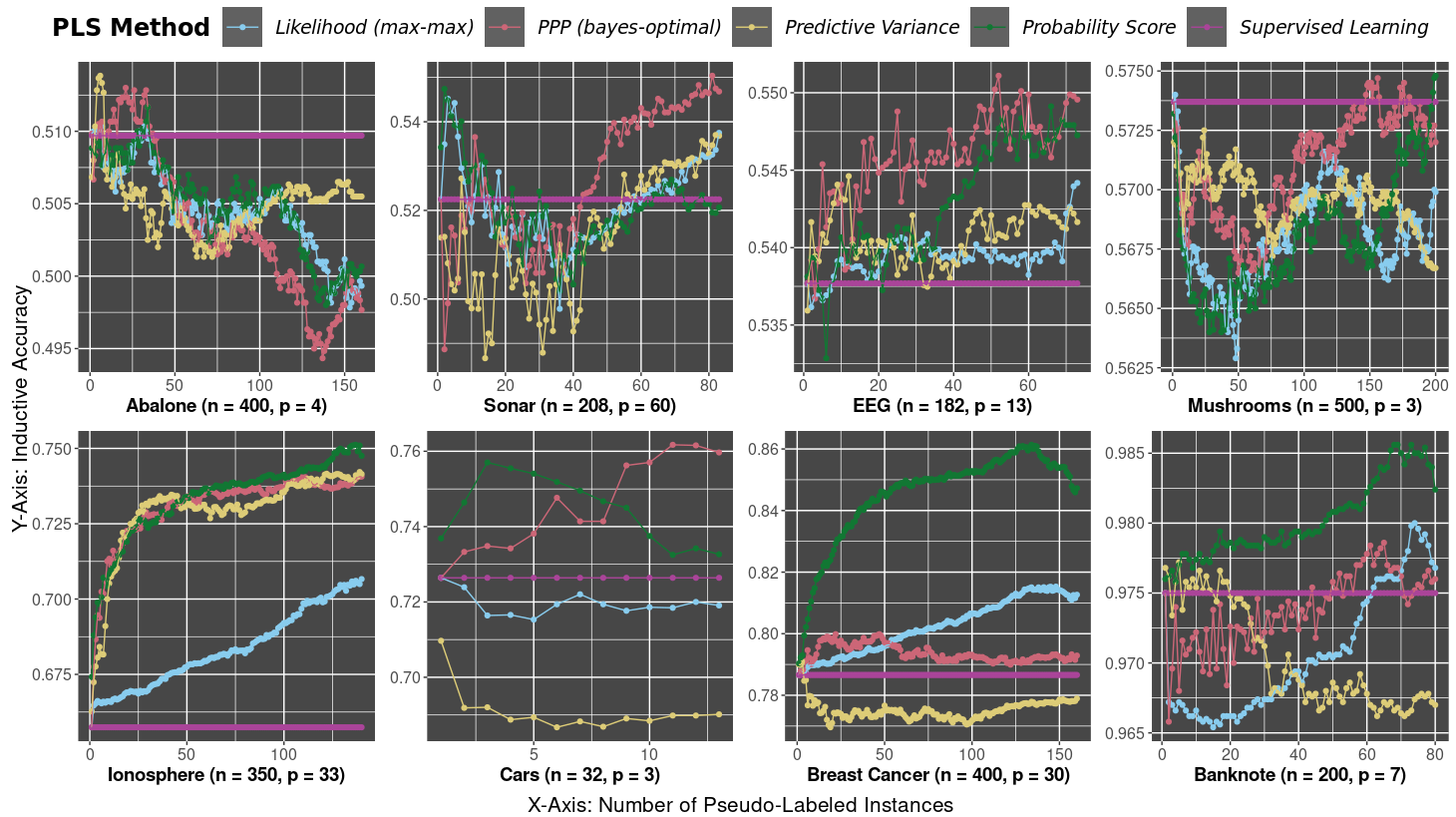
Experimental Setup: We formulate three hypotheses beforehand. Hypothesis 1 corresponds to the main motivation behind BPLS; its second part is a logical consequence thereof: If we are sceptical towards the initial model in case it generalizes well, we expect to select pseudo-labels in a worse way than when trusting the initial model. Hypothesis 2 is based on the decision-theoretic insights regarding PLS by the likelihood, see section 2.2: It embodies an optimistic reliance on the initial model and is thus expected to pick data that fits best into that model. We further expect (Hypothesis 3) BPLS to unambiguously outperform non-Bayesian selection methods in case the prior provides actual information about the data generating process – the latter is simply not available for non-Bayesian PLS. We benchmark semi-supervised (parametric) generalized linear models (GLMs) and (non-parametric) generalized additive models (GAMs) [Hastie and Tibshirani, 1987, Hastie, 2017] with PPP and pseudo-label likelihood against two common selection criteria (probability score and predictive variance) [Triguero et al., 2015] as well as a supervised baseline. For the latter, we abstain from self-training and only use the labeled data for training. Experiments are run on simulated binomially distributed data as well as on eight data sets for binary classification from the UCI repository [Dua and Graff, 2017]. The binomially distributed data was simulated through a linear predictor consisting of normally distributed features. Details on the simulations as well as on the data sets can be found in Supplement C and Supplement H. The share of unlabeled data was set to and . PLS methods were compared w.r.t. to (\sayinductive) accuracy of prediction on unseen test. All data sets were found to be fairly balanced except for the EEG data (minority share: ).
Results: Figures 1 and 2 as well as Table 1 summarize the results in the uninformative case (grey figures) for real-world and simulated data, respectively. \sayOracle stopping in Table 1 refers to comparing PLS methods with regard to their overall best accuracy as opposed to \sayfinal comparisons after the whole data set was labeled. Figure 2 sheds further light on results for simulated data, while Figure 3 displays results from benchmarking BPLS to classical PLS methods in the informative case (black figures). Detailed figures displaying results from all experiments can be found in the supplementary material.
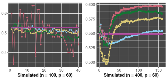
Interpretation: At first sight, comparing the accuracy gains in Figure 1 on different data sets (in order of ascending baseline performance) clearly supports Hypothesis 1: For harder tasks like EEG or sonar with relatively high ratio of features to data , Bayesian PPP outperforms traditional PLS, whilst being dominated by the probability score in case of easier tasks like banknote or breast cancer. For data sets with intermediate difficulty (mushrooms and ionosphere), PPP and other PLS methods compete head-to-head. The results on abalone data underpin a general fact in SSL (see section 1): Successful self-training requires at least some baseline supervised performance. Results on simulated data (Table 1) further support the role of in Hypothesis 1. Their visualization (Figure 2) nicely illustrates the inner working of selection by PPP: By not trusting the initial model, PPP affects the model’s test accuracy the most. While leaves some room for improvement through mitigating the overfitting by pseudo-labeled data, PPP leads to a noisy performance in case of close to . Here, even the final model still overfits. These promising results should not hide an inconsistency: The fact that PPP is superior on the cars task but not on the ionosphere task contradicts Hypothesis 1, since cars is harder than ionosphere, while having almost identical . We find Hypothesis 2 to be partially supported by the results. While 2 (a) holds for both the majority of simulated (see supplementary material) and real-world data (likelihood generally the closest to supervised performance), 2 (b) is challenged by considerable generalization performance gain on ionosphere and breast cancer data.
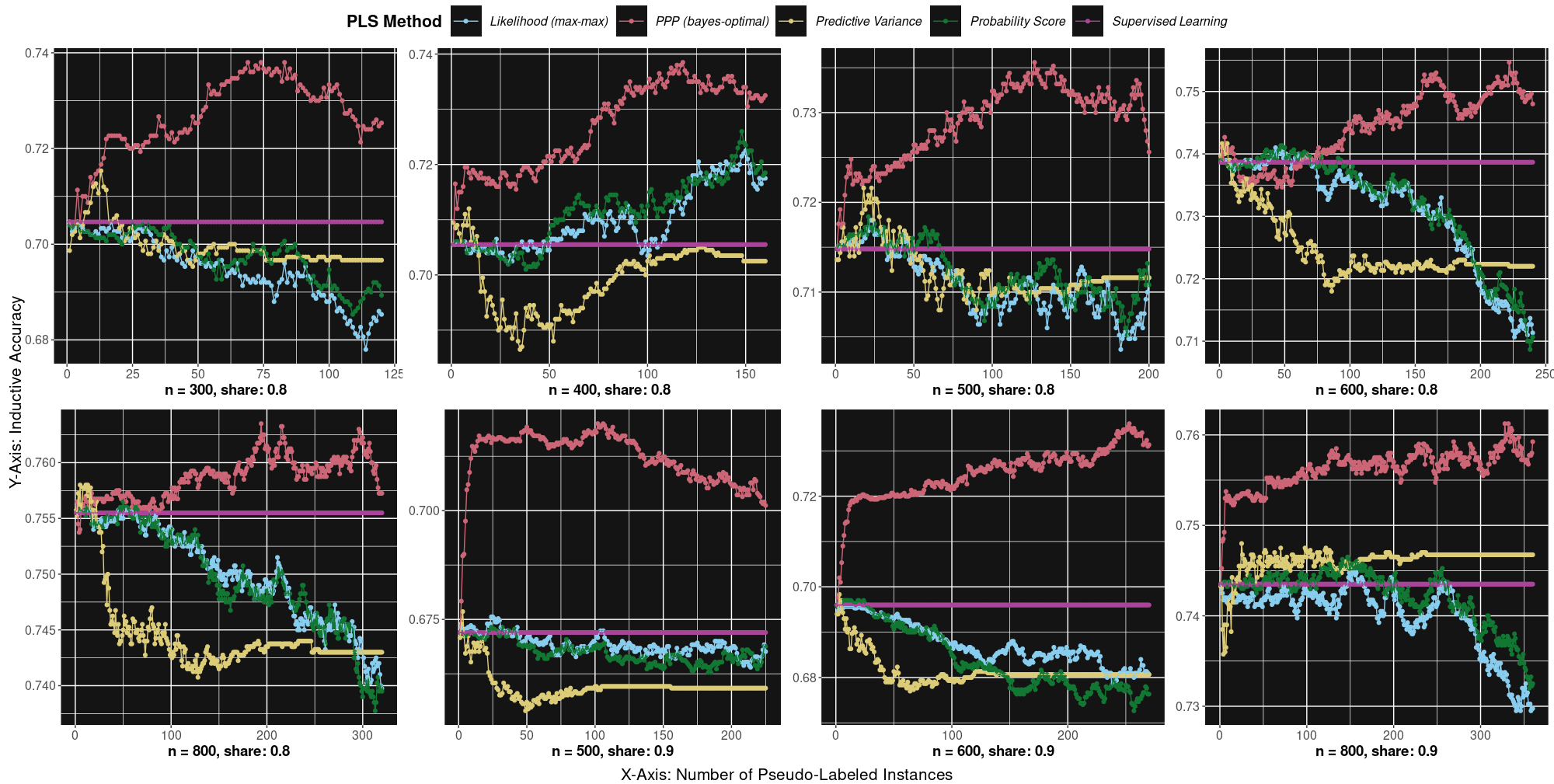
Figure 3 clearly supports Hypothesis 3: When using informative priors based on the true data-generating process, BPLS clearly outperforms traditional PLS methods. Results in Supplement D.3 further back this finding. This comes at no big surprise, since non-Bayesian PLS simply lack ways to incorporate such prior knowledge. From this perspective, the uninformative case (Hypothesis 1) corresponds to raising the bar and clearly is the theoretically more interesting benchmarking setup. However, many practical applications of SSL entail a myriad of pre-existing knowledge, e.g., radio spectrum identification [Camelo et al., 2019]. For practical purposes, thus, the informative situation might even be more relevant.
| n | q | ORACLE STOPPING | FINAL |
|---|---|---|---|
| 60 | 60 | PPP | PPP |
| 100 | 60 | PPP | Supervised Learning |
| 400 | 60 | PPP | PPP |
| 1000 | 60 | Probability Score | Probability Score |
5 RELATED WORK
Robust PLS: Robustness of PLS is a widely discussed issue in the self-training literature. [Aminian et al., 2022] propose information-theoretic PLS robust towards covariate shift. [Lienen and Hüllermeier, 2021] label instances in the form of sets of probability distributions (credal sets), weakening the reliance on a single distribution. [Vandewalle et al., 2013] aim at robustness to modeling assumptions by allowing model selection through the deviance information criterion during semi-supervised learning. [Rizve et al., 2020] propose uncertainty-aware pseudo-label selection which proves to compete with state-of-the-art SSL based on consistency regulation. The idea is to select pseudo-labeled instances whose probability score and predictive uncertainty are above (tunable) thresholds. The latter is operationalized by the prediction’s variance, and thus, unlike BPLS, fails to decompose approximation and modeling uncertainty, see Section 1. Both predictive variance and probability score serve as benchmarks in Section 4.
Bayesian Self-Training: There is a broad body of research on deploying Bayesian predictions in SSL and particularly in self-training [Gordon and Hernández-Lobato, 2020, Ng et al., 2018, Cai et al., 2011, Adams and Ghahramani, 2009]. The same holds for explicit likelihood-based inference, such as weighted likelihood [Sokolovska et al., 2008], conditional likelihood [Grandvalet and Bengio, 2004], and joint mixture likelihood [Amini and Gallinari, 2002]. Most of them use Bayesian models for predicting pseudo-labels. In contrast, we prove that the argmax of the PPP is the Bayes optimal selection of pseudo-labels given any predictive model. Regarding Bayesian or likelihood-based selection of pseudo-labels, there exists only little (Bayesian) or hardly any (likelihood-based) work. [Li et al., 2020] quantify the uncertainties of pseudo-labels by mixtures of predictive distributions of a neural net, applying MC dropout. This could be seen as an expensive MC-based approximation of the PPP. Very recently, [Patel et al., 2023] proposed PLS with regard to (a sampling-based approximation of) the entropy of the pseudo-labels’ posterior predictive distribution. The entropy is considered a measure of total uncertainty (aleatoric and epistemic) and often considered as regularization for PLS, see [Saporta et al., 2020, Liu et al., 2021] for instance. Abstaining from the entropy – as we do – effectively means not considering the aleatoric uncertainty. While including aleatoric uncertainty (e.g. measurement noise) generally makes sense, we consider it of minor importance in the concrete problem of initial overfitting, where we aim at disentangling epistemic uncertainty with regard to data and parameters: We want to choose pseudo-labels that are likely given the observed labeled data but not necessarily likely given the estimated parameters of the (over-)fitted model.
6 DISCUSSION
Extensions: We briefly discuss two venues for future work. The first extension loosens the restriction on one particular model class by performing model selection and PLS simultaneously. The idea would be to select these instances that can be best explained by the simplest learner (i.e., the one with least parameters). Further recall that both the framework of BPLS and our approximation of the PPP do not require data to be i.i.d distributed. Applying BPLS on dependent observations, such as in auto-correlated data like time series, is thus another promising line of further research.
Limitations: BPLS’ strength of being applicable to any learner can imply high computational costs in case of expensive-to-train models such as neural nets, because PPP approximations require refitting the model. Additionally, it might be difficult for practitioners to assess the risk of overfitting to the initial data set beforehand and opt for BPLS in response. Given the fact that BPLS is outperformed by traditional PLS in cases with no overfitting, this might be considered a drawback for practical application. However, Section 4 demonstrated that and the baseline supervised performance (both easily accessible) provide sound proxies for initial overfitting scenarios that can induce a confirmation bias in PLS. These proxies can (alongside cross-validation) help practitioners to identify such scenarios.
Conclusion: BPLS renders self-training more robust with respect to the initial model. This improves final performance if the latter overfits and harms it if not. Identifying overfitting scenarios is thus crucial for BPLS’ usage. What is more, BPLS allows incorporating prior knowledge, with the help of which substantial performance gains can be achieved. Besides, our insights from formalizing PLS as a decision problem clear the way for promising future work exploiting rich literature on Bayesian decision theory. Ultimately, we conclude that a Bayesian view can add great value not only to predicting but also to selecting data for self-training.
Acknowledgements
Thomas Augustin gratefully acknowledges support by the Federal Statistical Office of Germany within the co-operation project "Machine Learning in Official Statistics".
References
- [Abdar et al., 2021] Abdar, M., Pourpanah, F., Hussain, S., Rezazadegan, D., Liu, L., Ghavamzadeh, M., Fieguth, P., Cao, X., Khosravi, A., Acharya, U. R., et al. (2021). A review of uncertainty quantification in deep learning: Techniques, applications and challenges. Information Fusion, 76:243–297.
- [Adams and Ghahramani, 2009] Adams, R. P. and Ghahramani, Z. (2009). Archipelago: nonparametric Bayesian semi-supervised learning. In 26th International Conference on Machine Learning, pages 1–8.
- [Amini and Gallinari, 2002] Amini, M.-R. and Gallinari, P. (2002). Semi-supervised logistic regression. In 15th European Conference on Artificial Intelligence (ECAI 2002), pages 390–394.
- [Aminian et al., 2022] Aminian, G., Abroshan, M., Khalili, M. M., Toni, L., and Rodrigues, M. (2022). An information-theoretical approach to semi-supervised learning under covariate-shift. In International Conference on Artificial Intelligence and Statistics, pages 7433–7449. PMLR.
- [Andriushchenko and Flammarion, 2022] Andriushchenko, M. and Flammarion, N. (2022). Towards understanding sharpness-aware minimization. In International Conference on Machine Learning, pages 639–668.
- [Arazo et al., 2020] Arazo, E., Ortego, D., Albert, P., O’Connor, N. E., and McGuinness, K. (2020). Pseudo-labeling and confirmation bias in deep semi-supervised learning. In 2020 International Joint Conference on Neural Networks, pages 1–8. IEEE.
- [Barber, 2012] Barber, D. (2012). Bayesian reasoning and machine learning. Cambridge University Press.
- [Berger, 1985] Berger, J. O. (1985). Statistical decision theory and Bayesian analysis. Springer, Berlin., 2nd edition.
- [Cai et al., 2011] Cai, R., Zhang, Z., and Hao, Z. (2011). BASSUM: A Bayesian semi-supervised method for classification feature selection. Pattern Recognition, 44(4):811–820.
- [Camelo et al., 2019] Camelo, M., Shahid, A., Fontaine, J., de Figueiredo, F. A. P., De Poorter, E., Moerman, I., and Latre, S. (2019). A semi-supervised learning approach towards automatic wireless technology recognition. In 2019 IEEE International Symposium on Dynamic Spectrum Access Networks (DySPAN), pages 1–10.
- [Cattaneo, 2007] Cattaneo, M. E. (2007). Statistical decisions based directly on the likelihood function. PhD thesis, ETH Zurich.
- [Chapelle et al., 2006] Chapelle, O., Schölkopf, B., and Zien, A. (2006). Semi-supervised learning. Adaptive computation and machine learning series. MIT Press.
- [Dinh et al., 2017] Dinh, L., Pascanu, R., Bengio, S., and Bengio, Y. (2017). Sharp minima can generalize for deep nets. In International Conference on Machine Learning, pages 1019–1028. PMLR.
- [Dua and Graff, 2017] Dua, D. and Graff, C. (2017). UCI machine learning repository. http://archive.ics.uci.edu/ml.
- [Gauß, 1877] Gauß, C. F. (1877). Theoria motus corporum coelestium in sectionibus conicis solem ambientium, volume 7. FA Perthes.
- [Gordon and Hernández-Lobato, 2020] Gordon, J. and Hernández-Lobato, J. M. (2020). Combining deep generative and discriminative models for Bayesian semi-supervised learning. Pattern Recognition, 100:107156.
- [Grandvalet and Bengio, 2004] Grandvalet, Y. and Bengio, Y. (2004). Semi-supervised learning by entropy minimization. In Advances in Neural Information Processing Systems, volume 17.
- [Hastie, 2017] Hastie, T. (2017). Generalized additive models. In Chambers, J. M. and Hastie, T., editors, Statistical models in S, pages 249–307. Routledge.
- [Hastie and Tibshirani, 1987] Hastie, T. and Tibshirani, R. (1987). Generalized additive models: some applications. Journal of the American Statistical Association, 82(398):371–386.
- [Hüllermeier, 2014] Hüllermeier, E. (2014). Learning from imprecise and fuzzy observations: Data disambiguation through generalized loss minimization. International Journal of Approximate Reasoning, 55:1519–1534.
- [Hüllermeier and Waegeman, 2021] Hüllermeier, E. and Waegeman, W. (2021). Aleatoric and epistemic uncertainty in machine learning: An introduction to concepts and methods. Machine Learning, 110(3):457–506.
- [Łapiński, 2019] Łapiński, T. M. (2019). Multivariate Laplace’s approximation with estimated error and application to limit theorems. Journal of Approximation Theory, 248:105305.
- [Lee et al., 2013] Lee, D.-H. et al. (2013). Pseudo-label: The simple and efficient semi-supervised learning method for deep neural networks. In Workshop on challenges in representation learning, International Conference on Machine Learning, volume 3, page 896.
- [Li et al., 2018] Li, H., Xu, Z., Taylor, G., Studer, C., and Goldstein, T. (2018). Visualizing the loss landscape of neural nets. In Advances in Neural Information Processing Systems, volume 31.
- [Li et al., 2020] Li, S., Wei, Z., Zhang, J., and Xiao, L. (2020). Pseudo-label selection for deep semi-supervised learning. In 2020 IEEE International Conference on Progress in Informatics and Computing (PIC), pages 1–5. IEEE.
- [Lienen and Hüllermeier, 2021] Lienen, J. and Hüllermeier, E. (2021). Credal self-supervised learning. In Advances in Neural Information Processing Systems, volume 34, pages 14370–14382.
- [Liu et al., 2021] Liu, H., Wang, J., and Long, M. (2021). Cycle self-training for domain adaptation. In Advances in Neural Information Processing Systems, volume 34, pages 22968–22981.
- [Llorente et al., 2023] Llorente, F., Martino, L., Delgado, D., and Lopez-Santiago, J. (2023). Marginal likelihood computation for model selection and hypothesis testing: an extensive review. SIAM Review, 65(1):3–58.
- [Lotfi et al., 2022] Lotfi, S., Izmailov, P., Benton, G., Goldblum, M., and Wilson, A. G. (2022). Bayesian model selection, the marginal likelihood, and generalization. In International Conference on Machine Learning, pages 14223–14247.
- [Malinin and Gales, 2018] Malinin, A. and Gales, M. (2018). Predictive uncertainty estimation via prior networks. In Advances in Neural Information Processing Systems, volume 31.
- [McClosky et al., 2006] McClosky, D., Charniak, E., and Johnson, M. (2006). Effective self-training for parsing. In Proceedings of the Human Language Technology Conference of the NAACL, Main Conference, pages 152–159.
- [Miller, 2006] Miller, P. D. (2006). Applied asymptotic analysis, volume 75. American Mathematical Soc.
- [Murphy, 2012] Murphy, K. P. (2012). Machine learning: a probabilistic perspective. MIT press.
- [Ng et al., 2018] Ng, Y. C., Colombo, N., and Silva, R. (2018). Bayesian semi-supervised learning with graph gaussian processes. In Advances in Neural Information Processing Systems, volume 31.
- [Patel et al., 2023] Patel, G., Allebach, J. P., and Qiu, Q. (2023). Seq-ups: Sequential uncertainty-aware pseudo-label selection for semi-supervised text recognition. In Proceedings of the IEEE/CVF Winter Conference on Applications of Computer Vision, pages 6180–6190.
- [Rapoport, 1998] Rapoport, A. (1998). Decision theory and decision behaviour. Springer.
- [Rizve et al., 2020] Rizve, M. N., Duarte, K., Rawat, Y. S., and Shah, M. (2020). In defense of pseudo-labeling: An uncertainty-aware pseudo-label selection framework for semi-supervised learning. In International Conference on Learning Representations, 2020.
- [Rodemann et al., 2022] Rodemann, J., Kreiss, D., Hüllermeier, E., and Augustin, T. (2022). Levelwise data disambiguation by cautious superset classification. In International Conference on Scalable Uncertainty Management, pages 263–276. Springer.
- [Saporta et al., 2020] Saporta, A., Vu, T.-H., Cord, M., and Pérez, P. (2020). ESL: Entropy-guided self-supervised learning for domain adaptation in semantic segmentation. arXiv preprint arXiv:2006.08658.
- [Schwarz, 1978] Schwarz, G. (1978). Estimating the dimension of a model. The Annals of Statistics, 6(2):461–464.
- [Shi et al., 2018] Shi, W., Gong, Y., Ding, C., Tao, Z. M., and Zheng, N. (2018). Transductive semi-supervised deep learning using min-max features. In European Conference on Computer Vision, pages 299–315.
- [Sohn et al., 2020] Sohn, K., Berthelot, D., Carlini, N., Zhang, Z., Zhang, H., Raffel, C. A., Cubuk, E. D., Kurakin, A., and Li, C.-L. (2020). Fixmatch: Simplifying semi-supervised learning with consistency and confidence. In Advances in Neural Information Processing Systems, volume 33.
- [Sokolovska et al., 2008] Sokolovska, N., Cappé, O., and Yvon, F. (2008). The asymptotics of semi-supervised learning in discriminative probabilistic models. In 25th International Conference on Machine learning, pages 984–991.
- [Triguero et al., 2015] Triguero, I., García, S., and Herrera, F. (2015). Self-labeled techniques for semi-supervised learning: taxonomy, software and empirical study. Knowledge and Information systems, 42(2):245–284.
- [Van Engelen and Hoos, 2020] Van Engelen, J. E. and Hoos, H. H. (2020). A survey on semi-supervised learning. Machine Learning, 109(2):373–440.
- [Vandewalle et al., 2013] Vandewalle, V., Biernacki, C., Celeux, G., and Govaert, G. (2013). A predictive deviance criterion for selecting a generative model in semi-supervised classification. Computational Statistics & Data Analysis, 64:220–236.