Swapped goal-conditioned offline reinforcement learning

Abstract

Offline goal-conditioned reinforcement learning (GCRL) can be challenging due to overfitting to the given dataset. To generalize agent’s skills outside the given dataset, we propose a goal-swapping procedure that generates additional trajectories. To alleviate the problem of noise and extrapolation errors, we present a general offline reinforcement learning method called deterministic Q-advantage policy gradient (DQAPG). In the experiments, DQAPG outperforms state-of-the-art goal-conditioned offline RL methods in a wide range of benchmark tasks, and goal-swapping further improves the test results. It is noteworthy, that the proposed method obtains good performance on the challenging dexterous in-hand manipulation tasks for which the prior methods failed.

1 Introduction

Reinforcement learning (RL) has achieved remarkable success in a wide range of tasks, such as game playing (Mnih et al., 2013; Frazier & Riedl, 2019; Mao et al., 2022) and in robotics (Brunke et al., 2022; Nguyen & La, 2019). Goal-conditioned RL (GCRL) (Liu et al., 2022b; Chane-Sane et al., 2021; Andrychowicz et al., 2017) allows us to learn a more general RL agent which can reach an arbitrary goal without retraining. Although general policy learning is appealing, training goal-conditioned RL can be difficult. GCRL tasks usually have sparse rewards, and therefore the agent needs to explore the environment intensively, which is infeasible and dangerous in many real-world applications. On the other hand, offline RL has become a research hotspot in recent years as it learns the policy from offline datasets without endangering the real environment (Levine et al., 2020; Prudencio et al., 2022). The combination of offline RL and goal-conditioned RL takes the best of both worlds,

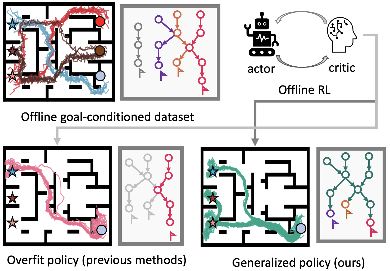
Figure 1: Illustration of the learned policy of our (below green) and previous (below red) offline GCRL learning. Our method learns a more general policy that reaches the goals from multiple states while the previous ones overfit to the training trajectories (top).

generalization and data efficiency, and is a promising approach for real-world applications (Ma et al., 2022).

The offline goal-conditioned RL (offline GCRL) meets two new challenges. At first, during training, the policy is likely to generate actions that are not present in the offline dataset. The value function cannot be correctly estimated for out-of-distribution actions. The biased value function causes the policy to deviate due to compounding errors (Levine et al., 2020). Prior works apply policy or value function constraints to solve the out-of-distribution problem. For example, the prior approaches constrain the policy to generate actions within the dataset or make value function updates conservatively. The constraints unfortunately limit the policy’s performance (Levine et al., 2020; Prudencio et al., 2022). The second challenge of offline GCRL is that each state can be assigned multiple goals, which means that the number of possible state-goal combinations can be extensive. Now general policy learning becomes difficult as the dataset covers only a limited state-goal observation space (Chebotar et al., 2021). To solve the offline GCRL learning problem, prior works apply hindsight labeling to generate positive goal-conditioned observations within all sub-sequences (Ghosh et al., 2019; Yang et al., 2022; Ma et al., 2022; Andrychowicz et al., 2017). However, hindsight relabelling has only limited positive impact on general skill learning, and the methods often learn an over-fitted goal-conditioned policy as shown in Figure 1. Chebotar et al. (2021) propose a goal-chaining technique to learn skills across trajectories, but it cannot handle the resulting noisy data properly (Ma et al., 2022).

In this work, we propose simple and efficient solutions to the challenges of offline GCRL: 1) goal-swapping, and 2) deterministic Q-Advantage policy gradient (DQAPG). Goal-swapping is a data augmentation technique that expands the dataset and thus provides a larger offline space to sample. DQAPG is an adaptive policy-constrained offline RL method that effectively learns from noisy samples. To summarize, our contributions are:

• We formulate a goal-swapping data augmentation technique, which enables an agent to learn more general skills through the given offline dataset trajectories.

• We propose an adaptive policy constraint offline RL method that learns a policy more effectively from noisy trajectories.

The proposed methods are evaluated on a wide set of offline GCRL benchmark tasks. The methods achieve superior performance compared to the available baselines, especially in the most challenging dexterous in-hand manipulation tasks.

2 Preliminaries

Goal-conditioned Markov decision process.  The classical Markov decision process (MDP) $\mathcal{M}$ is defined as a tuple $<\mathcal{S},\mathcal{A},\mathcal{T},r,\gamma,\rho_{0}>$, where $\mathcal{S}$ and $\mathcal{A}$ denote state space and action space, $\rho_{0}$ represents the initial states’ distribution, $r$ is the reward, $\gamma$ is the discount factor, and $\mathcal{T}$ denotes the state transition function  (Sutton & Barto, 2018). For goal-conditioned tasks, one additional vector $g$ specifies the goal that the agent should achieve. In general, the goal-conditioned RL augments MDP with the extra tuple $<\mathcal{G},p_{g},\phi>$, where $\mathcal{G}$ is the goal space and $p_{g}$ is the distribution of the desired task goals. $\phi:\mathcal{S}\rightarrow\mathcal{G}$ is a tractable mapping function that maps the state to a specific goal. The state-goal pair $(s,g)$ forms a new observation and is used as the input for agent $\pi(a|s,g)$. The goal-conditioned MDP (GC-MDP) is represented as $<\mathcal{S},\mathcal{G},\mathcal{A},\mathcal{T},r,\gamma,\rho_{0},p_{g}>$ (Liu et al., 2022b) (shown in Fig.2). The policy $\pi(a|s,g)$ makes decisions based on the state-goal pairs. The objective of GC-MDP can be formulated as:

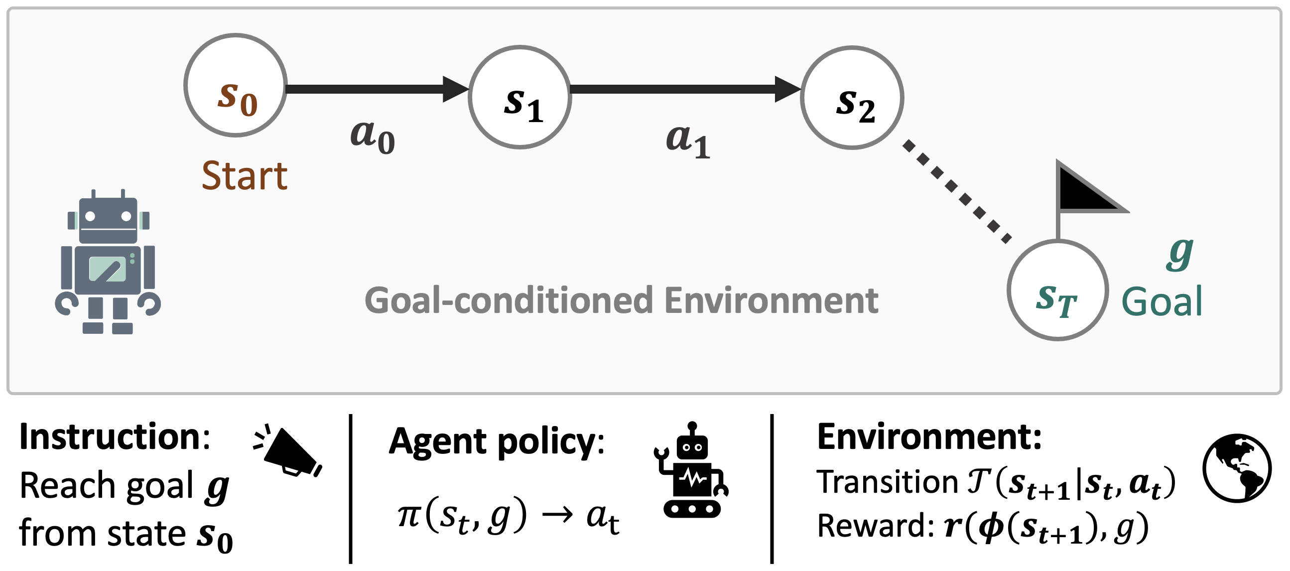
Figure 2: Visualization of the goal-conditioned Markov decision process (GC-MDP). Each state $s$ has a corresponding representation in the goal space $\eta=\phi(s)$.

$$\mathcal{J}(\pi)=\underset{a_{t}\sim\pi(\cdot|s_{t},g),g\sim p_{g},s_{t+1}\sim\mathcal{T}(\cdot|s_{t},a_{t})}{\mathbb{E}}\left[\sum_{t=0}^{\infty}\gamma^{t}r_{t}\right].$$ (1)

Two value functions are defined to represent the expected cumulative return, state-action value $Q$, and state value $V$. For GC-MDP, we have $V^{\pi}(s,g)$ function that is the goal-conditioned expected total discounted return from observation pair $(s,g)$ using policy $\pi$, and $Q^{\pi}(s_{t},a_{t},g)$ function estimates the expected return of an observation $(s_{t},g)$ for the action $a_{t}$ for the policy $\pi$. Furthermore, we have an advantage function $A^{\pi}(s,g,a)=Q^{\pi}(s,g,a)-V^{\pi}(s,g)$, which is another version of the Q-value but with lower variance. When the optimal policy $\pi^{*}$ is obtained, $Q^{*}(s,g,a)=V^{*}(s,g)$ (Sutton & Barto, 2018). In this work, we define a sparse reward

$$r(s,g)=\begin{cases}0,&\text{if }||\phi(s),g||<\epsilon\\ -1,&\text{otherwise}\end{cases},$$ (2)

where $||\phi(s),g||$ is a distance metric measurement, and $\epsilon$ is a distance threshold. We set the discount factor $\gamma=1$. In such case, $V(s,g)$ represents the expected horizon from state $s$ to goal $g$, and $Q(s,g,a)$ represents the expected horizon from state $s$ to the goal $g$ if an action $a$ is taken. This setting produces an intuitive objective: Find the policy that takes the minimum number of steps to achieve the task’s goal.

Offline goal-conditioned reinforcement learning.  Offline reinforcement learning (offline RL) is a specific problem of reinforcement learning where the agent cannot interact with the environment but only access a static offline dataset collected by unknown policies (Levine et al., 2020; Prudencio et al., 2022). The objective of offline goal-conditioned RL setting is the same as online goal-conditioned RL defined in Equation 1 but without interacting with the environment. Based on the definition of GC-MDP, we formulate the offline goal-conditioned RL dataset as $\mathcal{D}:=\{\mathbf{\zeta}_{i}\}_{i=1}^{N}$, where $\mathbf{\zeta}$ is the goal-conditioned trajectory and $N$ is the number of stored trajectories

$$\mathbf{\zeta}_{i}=\{<s_{0}^{i},\eta_{0}^{i},a_{0}^{i},r_{0}^{i}>,<s_{1}^{i},\eta_{1}^{i},a_{1}^{i},r_{1}^{i}>,$$

$$...,<s_{T}^{i},\eta_{T}^{i},a_{T}^{i},r_{T}^{i}>,g^{i}\}\enspace.$$

$\eta$ is the state’s corresponding goal representation calculated using $\eta_{t}=\phi(s_{t})$. The task goal $g^{i}$ is randomly sampled from $p_{g}$ and the initial state $s_{0}\sim\rho_{0}$. Note that the trajectories can be unsuccessful trajectories ($\eta_{T}^{i}\neq g^{i}$).

3 Challenges and related works

In this section, we discuss the challenges in the goal-conditioned offline RL setting. We first discuss the generalization issue and the importance of data utilization. About the offline RL aspect, we discuss the extrapolation problem and analyze the pros and cons of prior solutions.

3.1 Generalization power of goal-conditioned RL

Essentially, the objective of GCRL is to learn a general policy that can achieve all reachable goals (Liu et al., 2022b). The agent must learn a unified policy to perform multiple goals. However, the offline dataset state-goal pairs only cover a limited space of the goal-conditioned MDP. In other words, if we train a policy with the offline dataset, the policy learns to reach goals within a single trajectory in the dataset. This solution is not general, but undesirably specific. We present a more detailed discussion in Section 4.1. To learn a generalized goal-conditioned policy, the work actionable models (AM) (Chebotar et al., 2021) propose a goal-chaining technique that conducts goal-swapping augmentation. It assigns conservative values to the augmented out-of-distribution data for Q-learning. However, AM’s performance is limited when the dataset contains noisy data labels  (Ma et al., 2022). Besides goal-chaining, hindsight relabelling, or hindsight experience replay (HER), is also helpful in improving the sample efficiency for online goal-conditioned RLs (Andrychowicz et al., 2017; Yang et al., 2022). It relabels trajectory goals to states that were actually achieved instead of the task-commanded goals. Although HER efficiently utilizes the data within a single trajectory, it cannot connect different trajectories as goal-chaining does.

3.2 Offline reinforcement learning challenges

As arbitrary policies collect the offline dataset, applying off-policy methods for offline RL problems is intuitive. However, as the agent cannot access the environment, the off-policy RL usually faces distributional shift problems. The policy $\pi_{\psi}$ will likely generate actions that are not contained in the offline dataset. It makes Q-function unable to estimate the values correctly, resulting in bigger mistakes that compound once the policy diverges wildly from the dataset. This distributional shift issue is also called extrapolation error (Levine et al., 2020; Prudencio et al., 2022). Generally, researchers mainly propose three types of methods to solve offline RL problems (Prudencio et al., 2022): policy constraint methods, value function constraint methods, and one-step RLs. Policy constraint methods force the learned policy $\pi_{\psi}$ to stay close to the offline dataset’s behavioral policy $\pi_{D}$, either by explicitly sampling actions from $D$ (Fujimoto et al., 2019b; Wu et al., 2019) or minimizing certain divergence measurements between $\pi_{\psi}(\cdot|s)$ and $\pi_{D}(\cdot|s)$ (Kumar et al., 2019; Fujimoto & Gu, 2021; Peters & Schaal, 2007; Peng et al., 2020; Nair et al., 2020; Wang et al., 2020; Kostrikov et al., 2021a). Value constraint methods add regularization terms on the value function $Q$ to have a more conservative value estimation. It pushes up state-action pairs’ values in the dataset and pulls down the values in unseen actions (Kumar et al., 2020; Fujimoto et al., 2019a). In some challenging tasks (e.g., Kitchen tasks (Fu et al., 2021)), the value constraint approaches usually outperform policy constraint methods because the value function constraint approaches tend to be less conservative on policy than policy constraint methods. Some works also propose to use one-step on-policy RL to avoid extrapolation error. These works only do policy-evaluation on the offline dataset instead of on the policy. However, these methods can hardly learn the optimal value function due to the on-policy nature (Brandfonbrener et al., 2021; Kostrikov et al., 2021b; Ma et al., 2021).

In summary, the offline goal-conditioned RL not only faces extrapolation issues but also requires the policy to learn a generalizable policy that can reach all possible goals within the dataset. In this work, we aim to design a generalizable data-efficient offline RL solution for offline GCRL settings.

4 Method

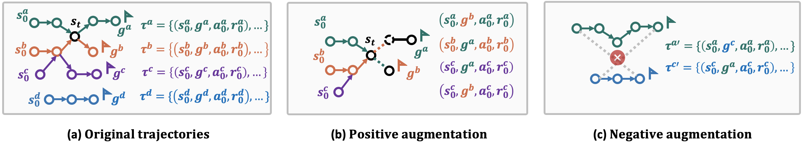
Figure 3: Example of the goal-swapping data augmentation. (a) original offline trajectories (denoted by four different colors). (b) augmentation example where the goals are reachable in each generated trajectory (positive augmentation). (c) negative augmentation where the goals are not anymore reachable.

To solve the challenges discussed in the previous section, we propose two simple yet effective methods: 1) goal-swapping augmentation and 2) deterministic Q-Advantage policy gradient (DQAPG). A schematic illustration of the methods inside the RL framework is Figure 4. The agent first conducts goal-swapping data augmentation to generate new state-goal pairs from the existing trajectories. Then DQAPG optimizes the policy from the augmented noisy data pairs. For this to work, we make an assumption that in the same environment, all goals are reachable from all states.

4.1 Goal-swapping data augmentation

As discussed in Section 3.1, the offline goal-conditioned dataset contains only a limited number of state-goal observations. Therefore, training with offline data often results in overfitted policies. An illustrative example is in Figure 3(a). In this example environment, the goals $g_{a}$ and $g_{b}$, are (forward) reachable from the three states $s_{0}^{a}$, $s_{0}^{b}$ and $s_{0}^{c}$. However, the original conditioned trajectories $\tau^{a}$ and $\tau^{b}$ limit the agent’s exploration to the known state-goal pairs $s_{0}^{a}\rightarrow g^{a}$, $s_{0}^{b}\rightarrow g^{b}$, and $s_{0}^{c}\rightarrow g^{c}$. Our goal-swapping (see Figure 6(b)) avoids the problem in an intuitive and simple-to-implement way.

To make the agent achieve as many goals as possible, we formulate a general goal-swapping augmented experience replay technique sketched in Algorithm 1. The algorithm randomly samples two trajectories and then swaps the goals between these two. In this way, it generates up to a combinatory number of new goal-conditioned trajectories. The dynamic programming nature of RL connects the state-goal pairs across different trajectories.

Goal-swapping analysis.  Let’s continue the example in Figure 3(a), where the goals $g\in[g^{a},g^{b},g^{c}]$ are reachable from the states $s\in[s_{0}^{a},s_{0}^{b},s_{0}^{c}]$ although not explicitly present in the offline dataset. However, if a goal is swapped between the original three trajectories $[\tau^{a},\tau^{b},\tau^{c}]$, the augmented goal-conditioned tuples shown in Figure 3(b) become available. The offline RL methods can chain the new trajectories thanks to the dynamic programming part of TD learning. Let’s take one value estimation as an example, $V(s_{t},g)=r+V(s_{t+1},g)$. For the pair $(s_{t+1},g)$, as long as $g$ is reachable and the value $V(s_{t+1},g)$ is well approximated, TD learning can backpropagate the state-goal (state-goal-action) values to the previous pairs. An illustration is in Fig.3(b), where the state $s_{t}$ is the ”hub state” shared by the three original trajectories and from which all goals $g^{i}\sim[g^{a},g^{b},g^{c}]$ are reachable. The values of these goal-conditioned states, $Q(s_{t},a_{t}^{i},g^{i})$, can be estimated and recursively backpropagated to $Q(s_{0},a_{0}^{i},g^{i}),i\in[a,b,c]$. Goal-swapping creates as many state-goal pairs as possible, so that TD learning ultimately backpropagates values over all trajectory combinations.

Although offline RL TD learning can connect goals across trajectories, applying the goal-swapping augmentation technique can be tricky. The reason is that the goal-swapping process is random, creating many non-optimal state-action pairs. Furthermore, those augmented state-action pairs may not even have a solution (the augmented goals are not reachable) within the offline dataset. This is demonstrated in Fig. 3(c). For this purpose, we rely on the actionable model (AM) (Chebotar et al., 2021), where Q-learning is heavily modified in a conservative Q-learning manner to handle the negative state-goal observations. This raises another problem as the performance of AM is very limited on noisy datasets (Ma et al., 2022).

Algorithm 1 Goal-swapping augmented experience replay

1:  Requiure: offline dataset as $D$, goal-conditioned tuples $\zeta$, state-goal mapping function $g_{i}=\phi(s_{i})$, and reward function $r=R(\phi(s),g)$.

2:  Sample goal-conditioned transitions $\zeta$ from $D$: $\zeta_{i}=\{g,s,a,r,s^{\prime}\}\sim D.$

3:  Sample random goals: $g_{rand}\sim D$

4:  Generate $\tau_{rand}$ by replacing $g$ with $g_{rand}$ in $\zeta$: $\zeta_{aug}=\{g_{rand},s,a,r_{aug},s^{\prime}\}$ where $r_{aug}=R(\phi(s^{\prime}),g_{rand})$

5:  Return $\zeta$ and $\zeta_{aug}$

4.2 Deterministic Q-Advantage policy gradient

To effectively learn from augmented offline data that inherently produces noisy data samples, we propose a deterministic Q-Advantage policy gradient method (DQAPG). The method is built upon the standard deterministic policy gradient (Silver et al., 2014). For better illustration, we denote the parameter of $V(s,g)$ as $\phi$, the parameter of $Q(s,g,a)$ as $\theta$ and $\pi(s,g)$ is parameterized by $\psi$.

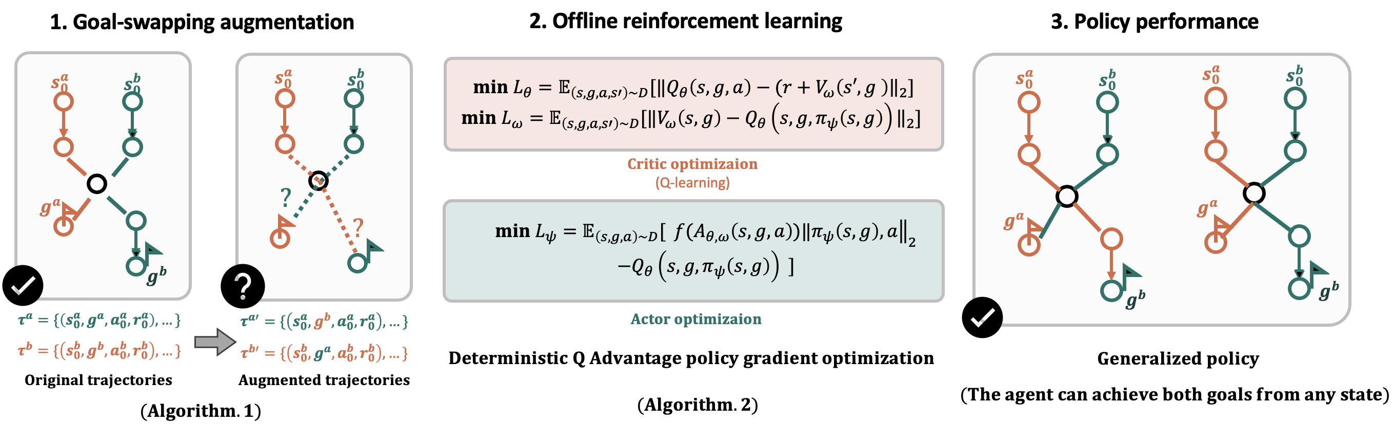
Figure 4: The schematic illustration of our framework. Firstly the goal-swapping data augmentation increases the amount of offline training pairs (Algorithms. 1). Then DQAPG then learns a general policy that can achieve different goals from the noisy training pairs (Algorithms. 2). Finally, the dynamic programming nature of Q-learning learns a policy to achieve all achievable goals within the dataset.

Value estimation.  We first aim at learning the optimal value $V_{\phi}(s)$ function and Q-function $Q_{\theta}(s,a)$ from the offline dataset. Based on the definition, the optimal $Q^{*}$ value equals to the optimal $V^{*}$ value (for the optimal policy $\pi^{\ast}$):

$$Q^{*}(s,a)=V^{*}(s)\enspace.$$

This indicates that $V(s,g)$ value function estimation can be added to the deterministic policy gradient (DPG) framework to learn the optimal $V^{*}$. Now we have the objective of the $V$ function learning:

$$L(\omega)=\underset{(s,g,a)\sim D}{\mathbb{E}}[\lVert V_{\omega}(s,g)-Q_{\theta}(s,g,\pi_{\psi}(s,g)){\rVert}_{2}]$$ (3)

and the corresponding objective of the $Q_{\theta}$ learning is

$$L(\theta)=\underset{(s,g,a,s^{\prime})\sim D}{\mathbb{E}}[\lVert Q_{\theta}(s,g,a)-(r+V_{\omega}(s^{\prime},g)){\rVert}_{2}]\enspace.$$ (4)

Based on the unity reward in Eq.  2, we set the optimization constraints $-H\leq V\leq 0$ and $-H\leq Q\leq 0$, where $H$ represents the maximum task horizon.

Policy optimization.  To suppress the extrapolation errors that can be dramatic in offline RL with generated data, we also constraint the policy similar to policy constraint offline RL methods. This is achieved by applying a regularization term that enforces $\pi_{\psi}(s,g)$ to be close to the actions stored in the dataset. This is implemented as the following offline RL objective (Nair et al., 2020; Peng et al., 2020):

$$\begin{split}\pi_{k+1}=\underset{\pi\in\Pi}{\operatorname*{arg\,max}}\underset{(s,g,s^{\prime})\sim D,a\sim\pi(s,g)}{\mathbb{E}}\left[\mathbb{Q}^{\pi_{k}}(s,g,a)\right]\\ \hbox{s.t.}~{}\operatorname*{KL}\left(\pi(\cdot|s,g)\lVert\pi_{D}(\cdot|s,g)\right)<\epsilon,\end{split}$$ (5)

where $\operatorname*{KL}$ is the KL-divergence and $\pi_{D}$ is a behavioral policy that is obtained using only the dataset samples $D$. $\mathbb{Q}$ can be the Q-function $Q(s,g,a)$ or the advantage function $A(s,g,a)$ (Prudencio et al., 2022; Sutton & Barto, 2018). However, different choices can result in different objectives. First, if we use the advantage function $A(s,g,a)$ as $\mathbb{Q}$ in Eq. 5, we can derive the following objective for a deterministic policy:

$$L(\psi)_{awbc}=\underset{(s,g,a)\sim D}{\mathbb{E}}[\exp(A^{\pi_{\psi}}(s,g,a))\\ \cdot\lVert\pi_{\psi}(s,g)-a{\rVert}_{2}].$$ (6)

If we choose to optimize $Q(s,g,a)$ in Equation 5, we have:

$$L(\psi)_{qbc}=\underset{(s,g,a)\sim D}{\mathbb{E}}[\lVert\pi_{\psi}(s,g)-a\rVert_{2}-Q^{\pi_{\psi}}(s,g,\pi_{\psi}(s))].$$ (7)

The details above can be found in Appendix A. The two objectives optimize the policy differently. The objective $L(\psi)_{awbc}$ is advantage-weighted behavioral cloning (BC), and is widely used in prior offline RL (Nair et al., 2020; Wang et al., 2020; Peng et al., 2020). However, such policy constraint tends to be more pessimistic as the actions in the dataset may not be the optimal goal-conditioned actions (Prudencio et al., 2022). The objective $L(\psi)_{qbc}$ optimizes the policy through deterministic policy gradient, similarly justified in (Fujimoto & Gu, 2021). It is worth noting that the two losses contribute to each other: the advantage weight ensures that the policy constraint is adaptive and selects good samples. Meanwhile, the $Q$ policy gradient guides the policy toward the best action. Based on their interoperation, we combine Equation 6 with Equation 7 to optimize the policy concurrently. This gives the final loss for policy updates

$$L(\psi)=\mathbb{E}_{(s,a)\sim D}[L_{awbc}(\psi)-\lambda Q_{\theta}(s,\pi_{\psi}(s),g)],$$ (8)

where the scalar $\lambda$ is defined as:

$$\lambda=\frac{1}{\frac{1}{N}\sum_{s_{i},g,a_{i}}|Q_{\theta}(s_{i},g,a_{i})|}$$

to balance between RL (in maximizing Q) and imitation (in minimizing the weighted BC term) (Fujimoto & Gu, 2021).

Algorithm 2 Q-Advantage policy gradient

  repeat

     Sample the transitions $\zeta$ and $\zeta_{aug}$ using Alg. 1.

     Train V-function $V_{\omega}$ by minimizing Eq. 3.

     Train Q-function $Q_{\theta}$ by minimizing Eq. 4.

     Optimize policy $\pi_{\psi}$ by minimizing Eq. 8.

  until Training is stopped

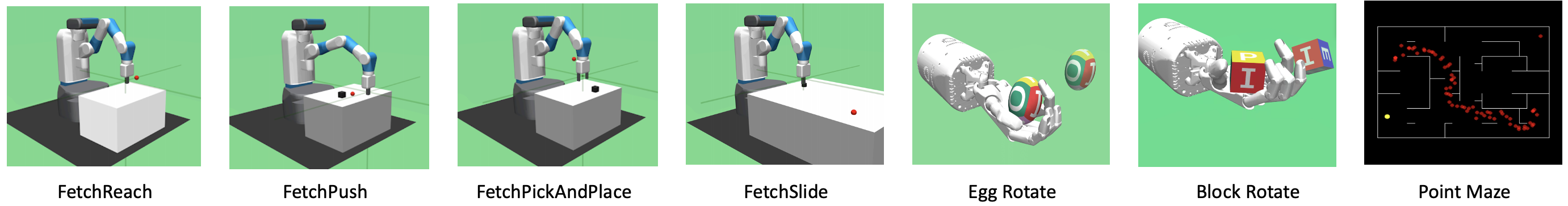
Figure 5: The goal-conditioned tasks selected for experiments in this work.

Table 1: Comparison of offline RL objectives. Note that function $w$ denotes the weighting function in WGCSL, $f^{\prime}_{\star}$ denotes the f-divergence function in GoFAR, $f$ denoted a monotonically increasing function such as exp, and $\sigma$ is the perturbation network in BCQ.

Offline goal-conditioned RL methods	Policy objective	Policy gradient	Weighted Regression
GCSL (Ghosh et al., 2019)	$\min_{\pi_{\psi}}\mathbb{E}_{(s,a,g)\sim D_{relabel}}[-\log\pi_{\psi}(a|s,g)]$	✗	✗
WGCSL (Yang et al., 2022)	$\min_{\pi_{\psi}}\mathbb{E}_{(s_{t},a_{t},g)\sim D_{relabel}}[-w(A(s_{t},g,a_{t}),t)\cdot\log\pi_{\psi}(a_{t}|s_{t},g)]$	✗	✓
GoFAR (Ma et al., 2022)	$\min_{\pi_{\psi}}\mathbb{E}_{(s,a,g)\sim D}[f^{\prime}_{\star}(R(s;g)+\gamma\mathcal{T}\mathcal{V}^{*}(s,a;g)-\mathcal{V}(s;g))\log\pi_{\psi}(a|s,g)]$	✗	✓
AM (Chebotar et al., 2021)	$\pi(a|s,g)=\underset{a\sim D}{\operatorname*{arg\,max}}Q^{*}(s,g,a)$	✗	✗
Offline RL methods	Policy objective	Policy gradient	Weighted Regression
AWR,AWAC, (Peng et al., 2020; Nair et al., 2020)	$\min_{\pi_{\psi}}\mathbb{E}_{(s,a,g)\sim D}[-\exp(A^{*}(s,g,a))\cdot\log\pi_{\psi}(a|s,g)]$	✗	✓
CRR (Wang et al., 2020)	$\min_{\pi_{\psi}}\mathbb{E}_{(s,a,g)\sim D}[-f(Q^{*}(s,g,a))\cdot\log\pi_{\psi}(a|s,g)]$	✗	✓
CQL (Kumar et al., 2020)	$\min_{\pi_{\psi}}\mathbb{E}_{{s,g}\sim D,a~{}\sim\pi_{\psi}}[-\log\pi_{\psi}(a|s,g)Q(s,g,a)]$	✓	✗
Onestep-RL, IQL (Brandfonbrener et al., 2021; Kostrikov et al., 2021b)	$\min_{\pi_{\psi}}\mathbb{E}_{(s,a,g)\sim D}[-\log\pi_{\psi}(a|s,g)Q^{\pi_{\psi}}(s,g,a)]$	✓	✗
BCQ  (Fujimoto et al., 2019b)	$\pi(a|s,g)=\underset{{a\sim[\operatorname*{VAE}(s,g)+\sigma_{\phi}(s,g,a)]}}{\operatorname*{arg\,max}}Q^{*}(s,g,a)$	✗	✗
TD3BC  (Fujimoto & Gu, 2021)	$\min_{\pi_{\psi}}\mathbb{E}_{(s,a,g)\sim D}[\lVert\pi_{\psi}(s,g)-a{\rVert}_{2}-Q(s,\pi_{\psi}(s,g),g)$	✓	✗
Ours	$\min_{\pi_{\psi}}\mathbb{E}_{(s,a,g)\sim D}[f(A(s,g,a))\lVert\pi_{\psi}(s,g)-a{\rVert}_{2}-Q(s,\pi_{\psi}(s,g),g)$	✓	✓

Algorithm summary.  The pseudo-code of the optimization steps of DQAPG is in Algorithm 2. The two main steps are i) sample and augment goal-conditioned tuples using Algorithm 1, and ii) then use the mixed augmented tuples $(\zeta,\zeta_{aug})$ in off-policy Q-Advantage policy gradient optimization. The weighted behavioral cloning $L(\psi)_{awbc}$ filters out the non-optimal goal-conditioned actions, and $Q(s,g,a)$ provides deterministic policy gradient to optimize the policy $\pi_{\psi}$.

4.3 Connection to prior works

Table 1 compares the proposed policy optimization objective to the prior works. For comparison, four state-of-the-art offline GCRL methods, and seven general offline conditioned RL methods were selected.

Table 1 shows that most of the prior GCRL methods are weighted regression-based approaches, which form an objective similar to Eq. 6. However, out of these GCSL (Ghosh et al., 2019) and WGCSL (Yang et al., 2022) can use only trajectories of successful examples, GoFAR (Ma et al., 2022) require that the offline dataset covers all reachable goals, and finally AM (Chebotar et al., 2021) fails on noisy trajectories. In contrast, the proposed method proposed avoids all these shortcomings.

On the other hand, our work shares the idea of the prior offline RL methods AWAC (Nair et al., 2020), CRR (Wang et al., 2020), and AWR (Peng et al., 2020). To properly acknowledge these prior works, we conclude that the proposed method takes advantage of both types of methods by jointly using the deterministic policy gradient optimization and the weighted regression. For the same reason, many of the above methods, in particular, AWAC, CRR, WGCSL, and GoFAR, can be integrated into our model.

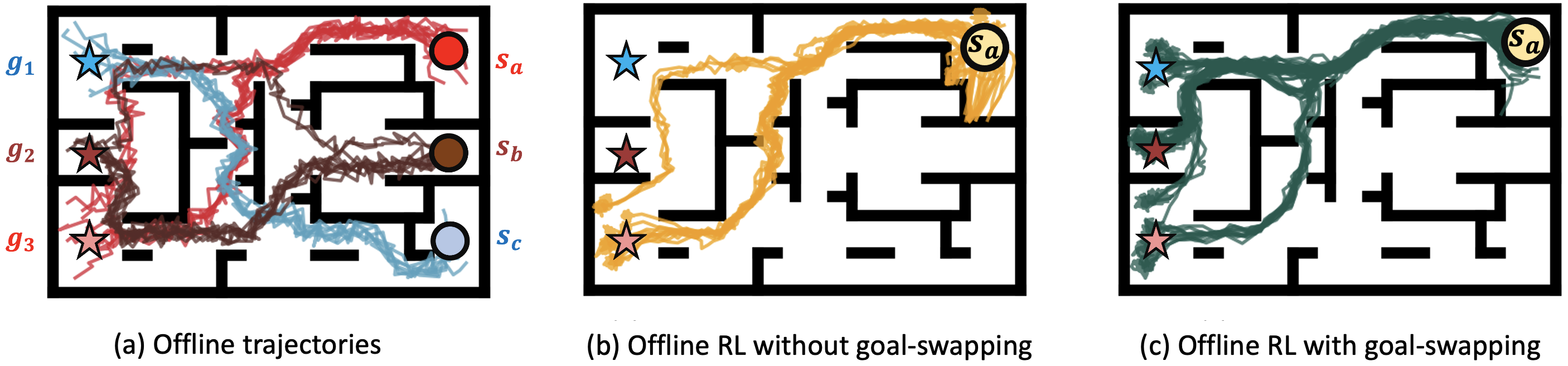
Figure 6: A PointMaze (toy) example. DQAPG was used and during the test time the agent always starts at $s_{0}$, and goal is randomply picked from $[g_{1},g_{2},g_{3}]$. (a) 3 types of offline trajectories: $s_{a}$ to $g_{3}$, $s_{b}$ to $g_{2}$, and $s_{c}$ to $g_{1}$. (b) offline RL performance without data augmentation (only one goal is achieved due to serious overfitting). (c) offline RL performance with goal-swapping augmentation.

Table 2: Evaluation of the goal-swapping augmentation in offline RL. The tested methods were trained without (*method*) and with (*method*-aug) the proposed augmentation. The performance metric is the average cumulative reward over 50 random episodes.     indicates that the augmented variant outperforms the original algorithm according to the t-test with p-value $<0.05$.

Datasize-small	FetchPush	FetchSlide	FetchPick	FetchReach	HandBlockZ	HandBlockParallel	HandBlockXYZ	HandEggRotate	PointMaze
DQAPG-aug	$\mathbf{29.06\pm 14.94}$	$2.0\pm 4.57$	$\mathbf{32.39\pm 12.45}$	$48.1\pm 0.94$	$31.69\pm 35.88$	$11.68\pm 19.8$	$20.49\pm 28.35$	$\mathbf{36.13\pm 33.9}$	$\mathbf{58.15\pm 19.83}$
DQAPG	$25.33\pm 17.71$	$1.25\pm 3.05$	$30.04\pm 14.79$	$48.14\pm 0.88$	$35.04\pm 35.85$	$16.8\pm 25.47$	$22.66\pm 28.27$	$34.08\pm 37.28$	$34.74\pm 30.16$
TD3BC-aug	$\mathbf{17.5\pm 15.47}$	$0.43\pm 1.48$	$29.68\pm 11.53$	$47.82\pm 2.28$	$\mathbf{19.1\pm 31.03}$	$2.61\pm 10.14$	$13.24\pm 25.24$	$\mathbf{33.27\pm 36.53}$	$\mathbf{51.26\pm 14.60}$
TD3BC	$12.94\pm 17.07$	$1.14\pm 4.78$	$28.86\pm 13.35$	$47.92\pm 1.07$	$17.25\pm 30.98$	$3.77\pm 13.4$	$12.76\pm 24.44$	$29.58\pm 36.62$	$28.00\pm 26.82$
AWAC-aug	$\mathbf{17.9\pm 15.82}$	$1.54\pm 3.79$	$12.49\pm 13.79$	$42.94\pm 4.02$	$\mathbf{13.86\pm 18.74}$	$0.26\pm 1.41$	$\mathbf{1.59\pm 7.64}$	$\mathbf{7.58\pm 10.03}$	$\mathbf{43.60\pm 25.44}$
AWAC	$15.11\pm 16.61$	$0.94\pm 2.3$	$12.19\pm 13.39$	$43.53\pm 3.56$	$0.93\pm 4.57$	$0.0\pm 0.0$	$0.5\pm 3.01$	$0.02\pm 0.18$	$32.12\pm 29.78$
IQL-aug	$3.5\pm 12.24$	$0.54\pm 4.56$	$1.26\pm 7.67$	$16.12\pm 17.01$	$1.45\pm 9.01$	$0.0\pm 0.0$	$0.34\pm 2.98$	$0.0\pm 0.0$	$\mathbf{20.72\pm 18.85}$
IQL	$3.73\pm 12.92$	$0.59\pm 4.55$	$1.32\pm 6.81$	$20.2\pm 18.2$	$1.43\pm 9.01$	$0.0\pm 0.0$	$0.18\pm 1.29$	$0.0\pm 0.0$	$14.45\pm 20.83$
Onestep-RL-aug	$\mathbf{27.38\pm 15.3}$	$0.22\pm 0.99$	$\mathbf{21.18\pm 17.51}$	$\mathbf{48.03\pm 1.44}$	$\mathbf{1.81\pm 6.07}$	$0.42\pm 4.63$	$0.09\pm 0.49$	$0.59\pm 1.86$	$0.73\pm 1.03$
Onestep-RL	$5.52\pm 11.94$	$1.12\pm 2.34$	$9.64\pm 14.86$	$45.9\pm 9.65$	$0.23\pm 1.61$	$0.0\pm 0.0$	$0.06\pm 0.63$	$0.01\pm 0.09$	$0.23\pm 1.45$
CRR-aug	$\mathbf{21.67\pm 15.52}$	$1.47\pm 3.53$	$16.73\pm 14.18$	$45.43\pm 2.18$	$0.34\pm 1.38$	$0.0\pm 0.0$	$0.25\pm 1.7$	$0.18\pm 0.95$	$\mathbf{44.83\pm 32.28}$
CRR	$16.5\pm 14.7$	$2.22\pm 5.67$	$15.98\pm 14.26$	$45.65\pm 2.2$	$0.73\pm 5.0$	$0.0\pm 0.0$	$0.4\pm 2.18$	$0.1\pm 1.07$	$26.32\pm 31.77$
CQL-aug	$\mathbf{31.18\pm 11.35}$	$\mathbf{4.97\pm 6.97}$	$\mathbf{24.65\pm 12.54}$	$44.6\pm 2.18$	$0.17\pm 0.79$	$0.0\pm 0.0$	$0.02\pm 0.18$	$0.0\pm 0.0$	$\mathbf{16.56\pm 28.14}$
CQL	$22.02\pm 17.24$	$1.92\pm 3.25$	$19.18\pm 13.74$	$44.15\pm 2.36$	$0.14\pm 0.66$	$0.0\pm 0.0$	$0.04\pm 0.32$	$0.0\pm 0.0$	$7.76\pm 18.42$

5 Experiments

The experiments in this section were designed to verify our main claims: 1) the goal-swapping augmentation helps to learn a more general policy; 2) the DQAPG improves the performance of goal-conditioned RL (GCRL); and 3) the method learns a working general policy from offline data.

Tasks.  Nine goal-conditioned tasks from (Plappert et al., 2018) were selected for the experiments. The tasks include the simple PointMaze task, four fetching manipulation tasks (FetchReach, FetchPickAndPlace, FetchPush, FetchSlide), and four dexterous in-hand manipulation tasks (HandBlock-Z, HandBlock-XYZ, HandBlock-Parallel, HandEgg). In the fetching tasks, the virtual robot should move an object to a specific position in the virtual space. In the four dexterous in-hand manipulation tasks, the agent is asked to rotate the object to a specific pose. The offline dataset for each task is a mixture of 500 expert trajectories and 2,000 random trajectories. The fetching tasks and datasets are taken from  (Yang et al., 2022). The expert trajectories for the in-hand manipulation tasks are generated similarly to (Liu et al., 2022a). For more details of the tasks, we refer to Appendix D.

Baselines.  The selected baseline methods are listed in Table.1. The HER ratio of 0.5 was used with all methods in all experiments. We trained each method for 10 seeds, and each training run uses 500k updates. The mini-batch size is 512. Complete architecture, hyper-parameter table, and additional training details are provided in Appendix B.

We used the cumulative test rewards from the environments as the performance metric in all experiments.

Table 3: DQAPG vs. the strong baselines for offline RL. No goal-swapping augmentation is used in this experiment.    indicates the best results according to the t-test with p-value $<0.05$.

	DQAPG	TD3BC	AWAC	IQL	Onestep-RL	CRR	BCQ	CQL
FetchPush	$25.33\pm 17.71$	$15.46\pm 17.59$	$15.11\pm 16.61$	$3.8\pm 12.72$	$4.26\pm 11.33$	$16.5\pm 14.7$	$3.78\pm 13.02$	$22.78\pm 15.77$
FetchSlide	$2.21\pm 5.6$	$0.84\pm 2.43$	$0.94\pm 2.3$	$0.53\pm 4.51$	$0.62\pm 1.66$	$2.22\pm 5.67$	$0.44\pm 4.47$	$1.95\pm 2.93$
FetchPick	$30.04\pm 14.79$	$29.1\pm 12.67$	$12.19\pm 13.39$	$1.67\pm 7.52$	$6.58\pm 12.3$	$15.98\pm 14.26$	$1.2\pm 7.65$	$21.02\pm 13.24$
FetchReach	$48.25\pm 0.86$	$47.95\pm 1.06$	$43.53\pm 3.56$	$21.76\pm 17.48$	$45.6\pm 10.14$	$45.65\pm 2.2$	$6.62\pm 12.62$	$44.54\pm 2.44$
HandBlock-Z	$35.04\pm 35.85$	$16.92\pm 30.81$	$0.93\pm 4.57$	$1.56\pm 8.53$	$0.22\pm 1.11$	$0.73\pm 5.0$	$1.88\pm 12.85$	$0.14\pm 0.66$
HandBlock-Parallel	$16.8\pm 25.47$	$3.5\pm 13.72$	$0.0\pm 0.0$	$0.22\pm 2.32$	$0.0\pm 0.0$	$0.0\pm 0.0$	$0.0\pm 0.0$	$0.0\pm 0.0$
HandBlock-XYZ	$22.66\pm 28.27$	$10.68\pm 22.71$	$0.5\pm 3.01$	$0.02\pm 0.2$	$0.02\pm 0.18$	$0.4\pm 2.18$	$0.78\pm 8.73$	$0.0\pm 0.0$
HandEggRotate	$35.08\pm 37.28$	$29.58\pm 36.62$	$0.02\pm 0.18$	$0.0\pm 0.0$	$0.01\pm 0.09$	$0.1\pm 1.07$	$0.0\pm 0.0$	$0.0\pm 0.0$
PointMaze	$34.74\pm 30.16$	$28.00\pm 26.82$	$32.12\pm 29.78$	$14.45\pm 20.83$	$0.0\pm 0.0$	$26.32\pm 31.77$	$0.0\pm 0.0$	$7.76\pm 18.42$

Table 4: Overall comparisons. The methods using goal-swapping augmentation are indicated in bold, and the methods in italic cannot use goal-swapping augmentation. highlights the best results according to the t-test with p-value $<0.05$.

DQAPG

TD3+BC

AM

WGCSL

GCSL

GoFAR

AWAC

IQL

Onestep-RL

CRR

BCQ

CQL

FetchPush

$30.36\pm 15.23$

$12.23\pm 15.63$

$19.29\pm 16.33$

$10.14\pm 16.19$

$8.98\pm 15.37$

$12.42\pm 16.58$

$8.05\pm 16.01$

$3.66\pm 12.92$

$11.96\pm 14.67$

$21.67\pm 15.52$

$3.82\pm 13.1$

$31.05\pm 11.41$

FetchSlide

$2.09\pm 4.8$

$0.95\pm 4.94$

$7.45\pm 11.41$

$2.03\pm 7.03$

$0.61\pm 1.79$

$1.75\pm 5.73$

$1.7\pm 6.03$

$0.29\pm 1.52$

$2.51\pm 5.02$

$1.47\pm 3.53$

$0.44\pm 4.47$

$4.94\pm 7.6$

FetchPick

$33.38\pm 10.86$

$27.34\pm 12.65$

$18.55\pm 19.08$

$6.56\pm 11.46$

$7.38\pm 12.07$

$16.39\pm 16.17$

$11.48\pm 13.98$

$0.88\pm 5.82$

$18.35\pm 18.74$

$16.73\pm 14.18$

$1.2\pm 7.65$

$25.4\pm 12.38$

FetchReach

$48.24\pm 0.85$

$47.81\pm 1.14$

$48.24\pm 0.86$

$36.96\pm 9.11$

$36.1\pm 9.35$

$45.15\pm 5.51$

$40.35\pm 11.39$

$17.21\pm 17.54$

$47.2\pm 6.43$

$45.43\pm 2.18$

$6.41\pm 12.49$

$44.38\pm 2.51$

HandBlock-Z

$31.69\pm 35.88$

$18.02\pm 30.14$

$0.65\pm 6.78$

$2.78\pm 11.34$

$3.08\pm 11.37$

$5.67\pm 16.17$

$14.38\pm 24.07$

$1.34\pm 8.9$

$1.31\pm 5.23$

$0.34\pm 1.38$

$2.26\pm 12.75$

$0.17\pm 0.79$

HandBlock-Parallel

$11.68\pm 19.8$

$2.04\pm 8.04$

$0.0\pm 0.0$

$0.02\pm 0.18$

$0.0\pm 0.0$

$0.01\pm 0.09$

$0.27\pm 2.03$

$0.0\pm 0.0$

$0.01\pm 0.09$

$0.0\pm 0.0$

$0.0\pm 0.0$

$0.0\pm 0.0$

HandBlock-XYZ

$20.49\pm 28.35$

$12.38\pm 22.54$

$0.04\pm 0.37$

$1.53\pm 7.89$

$0.34\pm 1.82$

$0.95\pm 5.01$

$0.03\pm 0.25$

$0.71\pm 5.47$

$0.12\pm 0.8$

$0.25\pm 1.7$

$0.73\pm 6.96$

$0.05\pm 0.38$

HandEggRotate

$36.13\pm 33.9$

$33.27\pm 36.53$

$0.0\pm 0.0$

$0.08\pm 0.89$

$1.18\pm 6.41$

$4.7\pm 14.81$

$8.42\pm 22.24$

$0.0\pm 0.0$

$0.59\pm 1.86$

$0.18\pm 0.95$

$0.0\pm 0.0$

$0.0\pm 0.0$

PointMaze

$58.15\pm 19.83$

$51.26\pm 14.60$

$0.24\pm 1.59$

$29.31\pm 21.78$

$26.78\pm 22.95$

$28.26\pm 32.25$

$43.60\pm 25.44$

$20.72\pm 18.85$

$0.0\pm 0.0$

$44.83\pm 32.28$

$0.0\pm 0.0$

$16.56\pm 28.14$

Goal-swapping experiment.  At first, for demonstration purposes, a qualitative demonstration of the goal-swapping augmentation is presented in Figure 6.

In this task, the test cases are different from the offline training data, and therefore it exemplifies the generalization power of the proposed augmentation technique. The offline training data was generated, by storing 10 trajectories from the three fixed paths: $s_{a}\rightarrow g_{3}$, $s_{b}\rightarrow g_{2}$, and $s_{c}\rightarrow g_{1}$ (visualized by different colors in Figure 6(a)). During testing, however, the starting point is fixed and goals were randomly sampled, thus representing unseen starting points and goal combinations. Two versions of the proposed DQAPG method were trained, one with the goal-swapping augmentation ($\star$-aug) and another without the augmentation. Each variant was tested using 50 random episodes.

The qualitative test results are shown in Figure 6(b) without augmentation and in Figure 6(c) with augmentation. These results indeed verify that the proposed augmentation technique is able to provide a more general policy that can generalize beyond its training data.

Next, we needed to verify that the augmentation technique itself generalizes to other tasks as well. The results for multiple methods and all nine task are shown in Table 2. The goal-swapping can benefit only methods using TD-learning, and therefore the following were selected for comparison: TD3+BC, AWAC, CRR, IQL, Onestep-RL, CQL, and our DQAPG.

This experiment provides an important finding, the goal-swapping augmentation does not provide significant negative effect if the task does not benefit from it, but in many cases it provides a significant performance boost. The tasks that benefit significantly from the augmentation were FetchPush and PointMaze. The tasks that obtained smaller improvements were FetchPick, HandBlockZ, and HandEggRotate. The rest of the tasks were more or less intact.

On the method side, AWAC seems to benefit the most from the augmentation (five tasks in total). All offline RL methods, except IQL, as well benefit from the augmentation. It seems that none of the methods benefit from the augmentation in two tasks, FetchSlide and HandBlockParallel. However, since the augmentation technique does not seem to have negative impact it is safe to be used.

DQAPG performance experiment.  It is essential to verify that the proposed DQAPG optimization objective is general and not problem specific. The offline RL results are summarized in Table 3. Overall, the DQAPG is the best in all nine tasks, and shares the best place in four tasks. It is worth noting that the basic TD3BC remains as a strong general baseline for offline goal-conditioned RL despite of its simplicity as compared to others. These results verify that the DQAPG’s objective function suits well for offline goal-conditioned RL. This setting is important in robotics where offline data provides superior sample efficiency and safety as compared to online learning with a real robot.

Offline goal-conditioned RL comparison.  In Table 4, are the results for the same tasks but using also the goal-swapping augmentation. The proposed augmentation technique indeed improves the performance of all methods (results without augmentation included for comparison). The goal-swapping augmentation was implemented on all TD-learning-based methods except GCSL, WGCSL, and GoFAR due to their own competing optimization objectives. Overall, the proposed method again performs the best. However, for the FetchSlide task, AM outperforms all other methods. It is worth noting that although TD3BC is a basic baseline for offline RL, it still outperforms many of the state-of-the-art GCRL methods such as WGCSL and GoFAR.

Almost all baselines failed for the challenging dexterous in-hand manipulation tasks (HandBlock-Parallel, HandBlock-Z, HandBlock-XYZ), for which the proposed method and data augmentation obtained the best performance.

6 Conclusion

In this work, we proposed a simple yet efficient offline goal-conditioned RL method, DQAPG, and a novel goal-swapping data augmentation technique. DQAPG deals better with noisy offline data than the existing methods, and the data augmentation technique allows offline RL methods to learn general policies beyond the provided offline samples. All findings were verified by extensive experiments on diverse offline learning tasks.

7 Limitations and Future work

The current form of goal-swapping augmentation is random and thus not necessarily efficient. More optimal swapping should be investigated. Another limitation is that DQAPG can learn only a deterministic policy. Nevertheless, the method can be converted to accept stochastic policies which are optimized using the re-parameterization trick. Another interesting research direction is to find methods to distinguish positive goal-swapping trajectories from negative (unreachable) ones.

Appendix A Algorithm Derivation Details

A.1 The advantage optimization objective

The most popular way to solve the distributional shift issue (extrapolation error) is to add policy constraints to the policy improvement update. In this section, we present the details of the objective in Eq.6 by strictly following work  (Peng et al., 2020). The optimization problem in goal-conditioned settings can be formulated as (Peng et al., 2020; Nair et al., 2020):

$$\underset{\pi}{\operatorname*{arg\,max}}=\int_{g}\rho_{D}(g)\int_{s}d_{D}(s|g)\int_{a}[A^{\pi}(s,g,a)]\textbf{{d}}a\textbf{{d}}s\textbf{{d}}g,\quad\int_{a}\pi(a|s,g)\textbf{{d}}a=1,\quad\textbf{s.t.}\operatorname*{KL}(\pi_{\psi}\lVert\pi_{D})\leq\epsilon,$$ (9)

where $\rho_{D}(g)$ represents the goal distribution in offline set $D$, and $d_{D}(s|g)=\sum_{t=0}^{\inf}\gamma^{t}p(s_{t}=s|\pi_{D},g)$ represents the goal-conditioned unnormalized discounted state distribution induced by the offline dataset policy $\pi_{D}$ (Sutton & Barto, 2018) , $\pi_{\psi}$ is the learned policy, $D$ is the offline goal-conditioned dataset, $\pi_{D}$ represents the behavioral policy that collects the dataset, $\mathcal{D(\lVert)}$ is some divergence measurement metric, $\epsilon$ is the threshold. We can enforce the KKT condition on Eq.9 and get the Lagrangian:

$$\begin{split}\mathcal{L}(\lambda,\pi,\alpha)=\int_{g}\rho_{D}(g)\int_{s}d_{D}(s|g)\int_{a}\pi(a|s,g)[A^{\pi}(s,g,a)]\textbf{{d}}a\textbf{{d}}s\textbf{{d}}g\\ +\lambda(\epsilon-\int_{g}\rho_{D}(g)\int_{s}d_{D}(s|g)\operatorname*{KL}(\pi_{\psi}\lVert\pi_{D})\textbf{{d}}s)\textbf{{d}}g\\ +\int_{s}\alpha(1-\int_{a}\pi(a|s,g)\textbf{{d}}a)\textbf{{d}}s\end{split}$$ (10)

Differentiating with respect to $\pi$ :

$$\frac{\partial\mathcal{L}}{\partial\pi}=p_{D}(s,g)A^{\pi}(s,g,a)-\lambda\cdot p_{D}(s,g)\cdot\log\pi_{D}(a|s,g)+\lambda p_{D}(s,g)\log\pi(a|s,g)+\lambda p_{D}(s,g)-\alpha$$

where $p_{D}(s,g)=\rho_{D}(g)d_{D}(s|g)$. Then set $\frac{\partial\mathcal{L}}{\partial\pi}$ to zero we can have

$$\pi(a|s,g)=\pi_{D}(a|s,g)\exp(\frac{1}{\lambda}A^{\pi})\exp(-\frac{1}{p_{D}(s,g)}\frac{\alpha}{\lambda}-1).$$ (11)

$\exp(-\frac{1}{p_{D}(s,g)}\frac{\alpha}{\lambda}-1)$ term is the partition function $Z(s,g)$ that normalizes a the goal-state conditional action distribution (Peng et al., 2020):

$$Z(s,g)=\exp(-\frac{1}{p_{D}(s,g)}\frac{\alpha}{\lambda}-1)=\int_{a}^{\prime}\pi_{D}(a^{\prime}|s,g)\exp(\frac{1}{\lambda}A^{\pi}(s,g,a^{\prime}))\textbf{{d}}a^{\prime}.$$ (12)

The closed-form solution can then be represented as:

$$\pi^{*}(a|s,g)=\frac{1}{Z(s,g)}\pi_{D}(a|s,g)\exp(\frac{1}{\lambda}A^{\pi}(s,g,a))$$ (13)

Finally, as $\pi$ is a parameterized function, we project the solution into the space of parametric policies and get the following optimization objective:

$$\begin{split}\underset{\pi}{\operatorname*{arg\,min}}\mathbb{E}_{s,g\sim D}[\operatorname*{KL}(\pi^{*}(\cdot|s,g)\lVert\pi(\cdot|s,g))]&=\underset{\pi}{\operatorname*{arg\,min}}\mathbb{E}_{s,g\sim D}[\operatorname*{KL}(\frac{1}{Z(s,g)}\pi_{D}(a|s,g)\exp(\frac{1}{\lambda}A^{\pi}(s,g,a))\lVert\pi(\cdot|s,g))]\\ &=\underset{\pi}{\operatorname*{arg\,min}}\mathbb{E}_{s,g\sim D}\mathbb{E}_{a\sim D}[-\pi(a|s,g)\exp(\frac{1}{\lambda}A^{\pi}(s,g,a))]\end{split}$$ (14)

Now this objective can be seen as weighted maximum likelihood. For a deterministic policy, the objective becomes:

$$\underset{\pi}{\operatorname*{arg\,min}}\mathbb{E}_{s,g,a\sim D}[\exp(\frac{1}{\lambda}A^{\pi}(s,g,a)\cdot\operatorname*{MSE}(\pi(s,g),a))$$ (15)

However, $Z(s)$ is always disregarded in practical implementations  (Peng et al., 2020; Nair et al., 2020). Especially the work (Nair et al., 2020) generally claims $Z(s,g)$ made performance worse. Thus we also ignored the term $Z(s)$ for practical implementation.

A.2 The Q optimization objective

If we choose to optimize $Q(s,g,a)$ in Eq. 5, we have the policy improvement objective:

$$\pi_{k+1}=\underset{\pi}{\operatorname*{arg\,max}}\,\mathbb{E}[Q^{\pi_{k}}(s,g,\pi_{k}(s,g))],\quad\int_{a}\pi(a|s,g)\textbf{{d}}a=1,\quad\textbf{s.t.}\operatorname*{KL}(\pi_{\psi}\lVert\pi_{D})\leq\epsilon.$$ (16)

As minimizing the KL-divergence is equal to minimizing the maximum likelihood (LeCun et al., 2015), and considering a deterministic policy, we have the following Lagrangian:

$$\begin{split}\mathcal{L}(\lambda,\pi)&=\mathbb{E}_{a\sim\pi(\cdot|s)}[Q^{\pi}(s,g,a)]+\lambda\mathbb{E}_{a,s,g\sim D}\operatorname*{MLE}(\pi(a|s,g))\end{split}$$ (17)

In this case, the deterministic policy $\pi(s,g)$ can be considered as a Dirac-Delta distribution thus, the $\int_{a}\pi(a|s,g)\textbf{{d}}a=1$ constraint always satisfies. The optimization objective is:

$$\underset{\pi}{\operatorname*{arg\,min}}\mathbb{E}_{s,g,a\sim D}[-Q^{\pi}(s,g,a)+\operatorname*{MSE}(\pi(s,g),a)]$$ (18)

Instead of finding a closed-form solution, this problem can be optimized through gradient descent. Based on the deterministic policy gradient theorem (Silver et al., 2014), $Q$ function directly provides gradients for policy optimization.

Appendix B Implementation Details

B.1 Offline RL technical details

DQAPG

As DQAPG is built upon the DPG framework, practically, we integrate our method into the TD3 framework (Fujimoto et al., 2018). In TD3, the double $Q$ networks and double $V$ networks can avoid the value overestimation issue. The detailed algorithm is presented in Algo.3 and Fig.9.

AM.

In actionable models’ work, the policy is represented as:

$$\pi(a|s,g)=\underset{a\sim D}{\operatorname*{arg\,max}}Q^{*}(s,g,a),$$

which only samples actions from the dataset and finds the action with maximum return. The objective of the value function is defined as:

$$\operatorname*{min}_{\theta}\mathbb{E}_{(s_{t},a_{t},s_{t+1},g)\sim{\mathcal{D}}}[((Q_{\theta}(s_{t},a_{t},g)-y(s_{t+1},g))^{2}+\mathbb{E}_{\tilde{a}\sim\mathrm{exp}(Q_{\theta})}[(Q_{\theta}(s,\tilde{a},g)-0)^{2}]]$$

where the TD target is:

$$y(s_{t+1},g)=\left\{\begin{array}[]{l l}{{1}}&{{\mathrm{if~{}}s_{t+1}=g}}\\ {{\gamma\mathbb{E}_{a\sim\pi}[Q(s_{t+1},a,g)]}}&{{\mathrm{otherwise.}}}\end{array}\right.$$

The first part of the loss $(Q_{\theta}(s_{t},a_{t},g)-y(s_{t+1},g))^{2}$ increases Q-values for reachable goals and the second part $\mathbb{E}_{\tilde{a}\sim\mathrm{exp}(Q_{\theta})}[(Q_{\theta}(s,\tilde{a},g)-0)^{2}$ regularizes the Q-function. When optimizing with gradient descent, the loss does not propagate through the sampling of action negatives $\tilde{a}\sim\exp$. We use the AM model that is implemented work (Ma et al., 2022). 10 random actions are sampled from the action-space to approximate this expectation. We keep the goal-chaining (goal-swapping) for all experiments. The hyperparameters are presented in Sec.B.2.

GoFAR, GCSL and WGCSL.

GCSL is a simple supervised regression method that does behavior cloning from hindsight relabelling dataset. Thus we only use the policy network from TD3 and optimize it with maximum likelihood loss. We refer the objective to Table 1. The WGCSL is implemented on top of GCSL, incorporated with TD3. More specifically, the policy objective is:

$$\min_{\pi}\mathbb{E}_{(s_{t},a_{t},g)\sim D_{relabel}}[-\gamma^{t-i}A_{wgcsl}^{\pi}(s_{t},g,a_{t})\cdot\log\pi(a_{t}|s_{t},g)],$$

where $i$ represents the hindsight relabelling steps in the future. The advantage weighting in the regression loss is the TD error

$$A_{wgcsl}^{\pi}(s,g,a)=r+Q^{\pi}(s^{\prime},g,\pi(s^{\prime},g))-Q(s,g,a),\quad a\sim D.$$

As AM, GoFAR, WGCSL and GCSL are fine-tuned in work (Ma et al., 2022), we keep the same implementations for this work https://github.com/jasonma2016/gofar.

BCQ

The goal-conditioned objective function of BCQ in this work is as follows:

$$\pi(a|s,g)=\underset{{a\sim[\operatorname*{VAE}(s,g)+\sigma_{\phi}(s,g,a)]}}{\operatorname*{arg\,max}}Q^{*}(s,g,a)$$

where $\sigma_{\phi}(s,g,a)$ is the goal conditioned perturbation model, which disturbs the action within a range between $[-\Phi,\Phi]$. The generative model $\operatorname*{VAE}(s,g)$ generates the actions that fit the offline dataset’s distribution. The Q function is learned using the Clipped Double Q-learning in TD3 (Fujimoto et al., 2018). The policy is implicitly presented as the above equation: sample the actions within the dataset with the maximum return. All hyperparameters are kept the same as the original work (Fujimoto et al., 2019b). The only difference is that we have an additional goal as input. In this work, we implemented BCQ based on its official source code https://github.com/sfujim/BCQ.

CQL

In work CQL, the constrain $\operatorname*{KL}(\pi(\cdot|s,g)\lVert\pi_{D}(\cdot|s,g))$ is added on value function instead of directly on policy. The loss of the value function can be written as:

$$\begin{split}L_{CQL}=\alpha\mathbb{E}_{(s_{t},g)\sim D}\big{[}\log\sum_{a}\exp(Q(s_{t},a,g))-\mathbb{E}_{a\sim\pi_{b}(\cdot|s_{t},g)}|Q(s_{t},a,g)\big{]})\\ +\;\frac{1}{2}\mathbb{E}_{(s_{t},a_{t},s_{t+1},g)\sim D}\left[(Q(s_{t},a_{t},g)-\mathcal{B}^{\pi}Q(s_{t},a_{t},g))^{2}\right],\end{split}$$ (19)

where $\pi_{b}$ is the behavior policy that collects offline dataset $D$ and $\mathcal{B}^{\pi}$ is the Bellman operator. The policy objective of CQL is a typical policy gradient objective, which is formulated as:

$$\min_{\pi}\mathbb{E}_{{s,g}\sim D,a~{}\sim\pi(\cdot|s,g)}[-\log\pi_{\psi}(a|s,g)Q^{\pi}(s,g,a)]$$

All hyperparameters are kept the same as the original work (Fujimoto et al., 2019b). The only difference is that we have an additional goal as input. The technical implementation is based on the official code https://github.com/aviralkumar2907/CQL.

CRR

The idea of CRR is to use $Q(s,a,g)$ to weight the behavior cloning, and the policy objective is :

$$\underset{\pi}{\operatorname*{arg\,max}}\mathbb{E}_{s,a,g\sim D}[f(Q^{\pi}_{\theta},\pi,s,a)\,\mathrm{log}\,\pi(a|s,g)],$$

where $f$ is a non-negative, scalar, monotonically increasing function in $Q_{\theta}$. In this work, we choose to use:

$$f=\mathbb{I}[A^{\pi}(s,g,a)>0]$$

as it has the best performance in the original implementation. $\mathbb{I}$ is the indicator function. Our CRR is implemented based on https://github.com/takuseno/d3rlpy, and all hyperparameters are kept the same as the original work (Wang et al., 2020).

AWAC

The work AWAC shares a similar idea as CQL, but it uses the advantage function to weight the regression. Its policy objective is:

$$\underset{\pi}{\operatorname*{arg\,max}}\mathbb{E}_{s,a,g\sim D}[\exp(A_{\theta}^{\pi}(s,g,a)\,\mathrm{log}\,\pi(a|s,g)],$$

and the advantage value is the TD error:

$$A^{\pi}_{\theta}(s,g,a)=r+Q^{\pi}_{\theta}(s^{\prime},g,a^{\prime})-Q^{\pi}_{\theta}(s,g,a),\quad a\sim D,a^{\prime}\sim\pi(\cdot|s,g).$$

. Our CRR is implemented based on https://github.com/takuseno/d3rlpy.

Onsetep-RL, IQL

The idea of Onestep-RL is only learning $Q^{\pi_{D}}$ instead of $Q^{*}$. It means that the algorithm only conducts policy evaluation based on offline dataset $D$ once, and use the estimated value functions to optimize $\pi$  (Brandfonbrener et al., 2021). In such case, we can write the policy objective as:

$$\underset{\pi}{\operatorname*{arg\,max}}\mathbb{E}_{s,g\sim D,a\sim\pi(\cdot|s,g)}[\exp(A_{\theta}^{{\color[rgb]{1,0,0}{\pi_{D}}}}(s,g,a)\,\mathrm{log}\,\pi(a|s,g)],$$

where ${\color[rgb]{1,0,0}{\pi_{D}}}$ is the behavior policy that collects dataset $D$. To improve the performance of Onestep-RL, the work IQL proposes using an expectile regression loss for policy evaluation, which is defined as:

$$\mathcal{L}^{\tau}_{2}(x)=\begin{cases}(1-\tau)x^{2},&\text{if }x>0\\ \tau x^{2},&\text{otherwise}\end{cases},$$

where $\tau$ represents the expectile. In this way, IQL considers $V^{\tau}(s,g),Q^{\tau}(s,g,a),A^{\tau}(s,g,a)$ as the best values from the actions within the support of offline data  (Kostrikov et al., 2021b). The IQL has the same policy objective as Onestep-RL, and its value function objective can be written as:

$${\cal L}_{V}(\omega)=\mathbb{E}_{(s,g,a)\sim D}[\mathcal{L}_{2}^{\tau}(Q_{\theta}(s,a)-V_{\omega}(s))]$$

$${\cal L}_{Q}=\mathbb{E}_{(s,g,a,s^{\prime})\sim D}[(r(s,g,a)+\gamma V_{\omega}(s,g)-Q_{\theta}(s,g,a))^{2}]$$

Note that when the $\tau=0.5$, IQL is identical to Onestep RL. In this work, we choose $\tau=0.75$ as it has the best performance (Kostrikov et al., 2021b). We use the official implementation in this work  https://github.com/ikostrikov/implicit_q_learning.

B.2 Hyperparameters

In this work, DQAPG, GCSL, WGCSL, GoFAR, CRR, AWAC, Onestep-RL, IQL, AM, TD3BC share the same network architectures. The hyperparameters of these methods are presented in Table.5. In work (Ma et al., 2022), GoFAR, WGCSL, GCSL, and AM’s parameters have already been fine-tuned for goal-conditioned tasks. Thus we keep the hyperparameters as implemented in  (Ma et al., 2022). For BCQ and CQL implementation, we keep the same hyperparameters used in their original works  (Fujimoto et al., 2019b; Kumar et al., 2020).

Table 5: General hyperparameters of networks

Hyperparameter	Value
Number of layers ($\pi$, $Q$, $V$ )	3
Size of hidden layers ($\pi$, $Q$, $V$)	256
Activation functions ($\pi$, $Q$, $V$)	ReLU
Batch size	512
Learning rate	$10^{-3}$
Polyak average weight	0.95
Target network update steps	10
Hindsight relabelling ratio	0.5

Appendix C Task details

C.1 Fetch Tasks

For Fetch tasks, the environments are based on the 7-DoF Fetch robotics arm, which has a two-fingered parallel gripper. The robot action frequency is set as $25Hz$  (Plappert et al., 2018). The state includes 1) the object’s Cartesian position and rotation using Euler angles, 2) its linear and angular velocities, and 3) its position and linear velocities relative to the gripper. A goal is considered achieved if the distance between the block’s position and its desired position is less than 1 cm. The environment’s original binary reward is defined as

$$r=\begin{cases}1,&\text{if }distance\,\,<1cm\\ 0,&\text{otherwise}\end{cases}.$$ (20)

The environment’s original binary reward is used for task performance evaluation (Section  5).

• FetchPickAndPlace In this task, the task is to grasp the object and move it to the target location. The target location is randomly sampled in the space (e,g., on the table or above it). The goal is 3-dimensional and describes the desired position of the object.

• FetchPush In this task, a block is placed in front of the robot. The robot can only push or roll the object to the target position. The goal is 3-dimensional and describes the desired position of the object.

• FetchSlide The task is to move a block to a target position. The block is put on a long slippery table, and the target position cannot be reached by the robot. The robot must hit the block so it can slide to the target position. The goal is 3-dimensional and describes the desired position of the object.

• FetchReach In this task, the robot is required to move its end-effector to a specific position. The goal is 3-dimensional and describes the desired position of the end-effector.

C.2 In-hand manipulation tasks

For in-hand manipulation tasks, the environments are based on s an anthropomorphic robotic hand with 24 degrees of freedom. The observation includes 24 positions and velocities of the robot’s joints, a quaternion representation of the manipulated object’s linear and angular velocities. The actions are implemented as absolute position control, which is 20-dimensional. The action frequency is set to $25\mathrm{Hz}$. In these tasks, an object is placed on the palm of the hand, and the task is to manipulate the block to reach the target pose. The goal is 7-dimensional and includes the target position (in Cartesian coordinates) and target rotation (in quaternions). No target position is given in all tasks. A goal is considered achieved if the distance between the object’s rotation and its desired rotation is less than 0.1 rad. The environment’s original binary reward is defined as

$$r(s,g)=\begin{cases}1,&\text{if }rotation\,\,difference\,\,<\,\,1rad\\ 0,&\text{otherwise}\end{cases}.$$ (21)

The environment’s original binary reward is used for task performance evaluation (Section  5).

• HandManipulationBlockRotateZ The task is to manipulate the block to a random target rotation around the z-axis of the block.

• HandManipulationBlockParallel The task is to manipulate the block to a random target rotation around the z-axis of the block and axis-aligned target rotations for the x and y axes.

• HandManipulationBlock The task is to manipulate the block to a random target rotation for all axes of the block.

• HandManipulationEggRotate The task is to manipulate the egg-like object to a random target rotation for all axes of the egg.

C.3 PointMaze

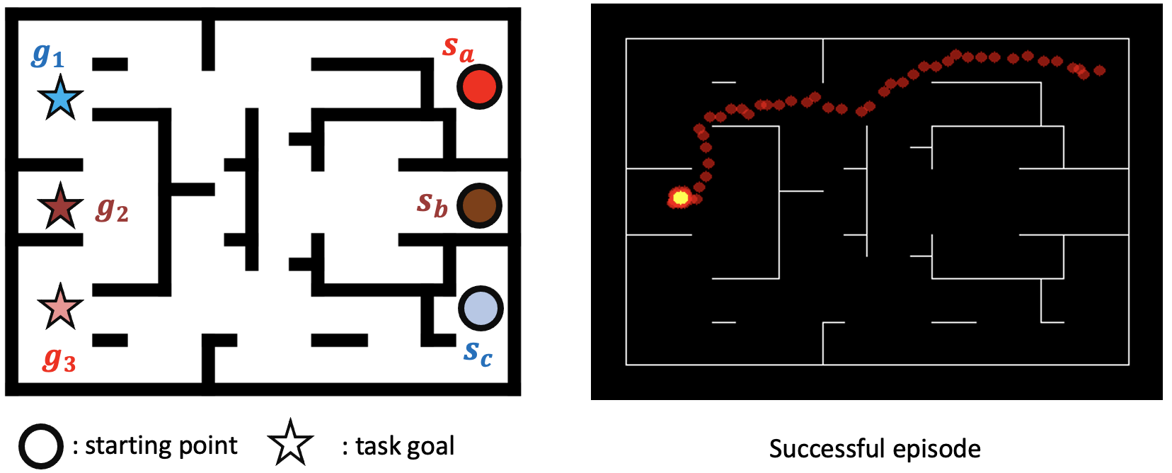
Figure 7: PointMaze environment. The left figure illustrates the task settings. There are 3 starting points and 3 task goals. The right figure presents one successful trajectory generated by an expert.

We further implemented a customized continuous 2D PointMaze. In this environment, the agent is randomly placed at a starting point $s_{0}\sim[s_{a},s_{b},s_{c}]$, and the task goal is randomly chosen from goal clusters $g\sim[g_{1},g_{2},g_{3}]$. Specifically, each starting point $s\in[s_{a},s_{b},s_{c}]$ shown in Figure 7 represents a cluster of points, and so do the goal points. The maze size is $24\times 18$. A goal is considered achieved if the euclidean distance is smaller than 2. The observation is the agent’s position in this maze $(x,y)$, and the action is in the range $(2,2)$. We use this task to visualize the generalizability problem faced by goal-conditioned reinforcement learning.

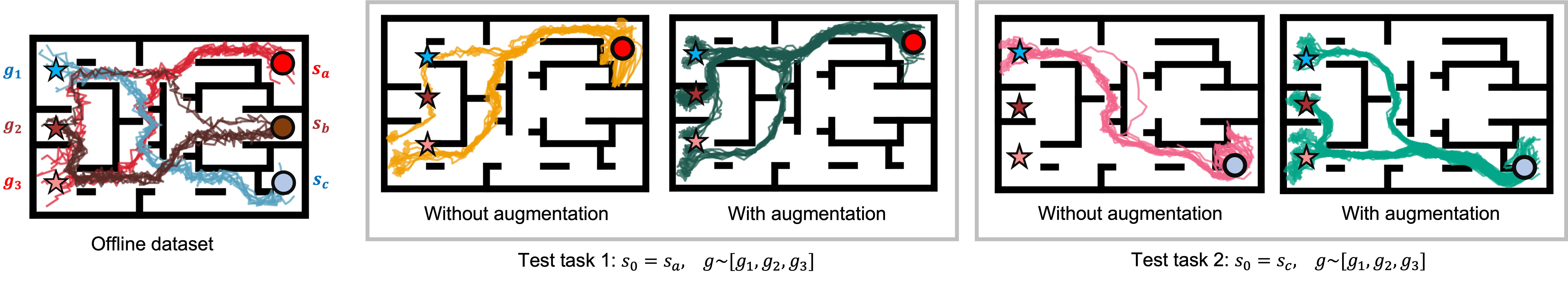
Figure 8: The PointMaze visually presents the generalizability issue of offline goal-conditioned RL. Without goal-swapping augmentation, the offline RL only learns an overfitted policy.

Appendix D Dataset collection

PointMaze. 

We used $\mathrm{A}^{*}$ as an expert to generate the offline dataset for GCRL. We add random action noise on the expert-planned trajectories to generate sub-optimal training data. As is discussed in Sec.5, only three types of goal-conditioned trajectories are collected, in total 30 trajectories.

Fetch tasks. 

For the Fetch tasks, we use the dataset collected in work WGCSL (Yang et al., 2022), which is generally used as goal-conditioned offline RL benchmarks (Ma et al., 2022). For each task, the original dataset contains 40K expert trajectories and 40K trajectories collected by random policy. As we address the data-efficiency and generalizability problem, in this work we only take 500 expert trajectories and 2K random trajectories to form a new offline GCRL dataset. The original dataset is provided by WGCSL in https://github.com/YangRui2015/AWGCSL.

In-hand manipulation tasks. 

In-hand manipulation tasks are challenging tasks that no dataset was provided in the previous offline GCRL works. We use the MRN method provided in  (Liu et al., 2022a) to collect the expert trajectories for all in-hand manipulation tasks. 500 expert trajectories and 2K random trajectories are collected for each task. More specifically, the implementation code of the expert policy can be found here https://github.com/Cranial-XIX/metric-residual-network.

Appendix E Source code

First, we illustrate the full pseudo-code of our algorithms. We also attach our source code of DQAPG in this section. We use Pytorch 1.13.1 for implementation. The core code is presented in Figure 9, and the full pseudo-code is presented in Algo.3.

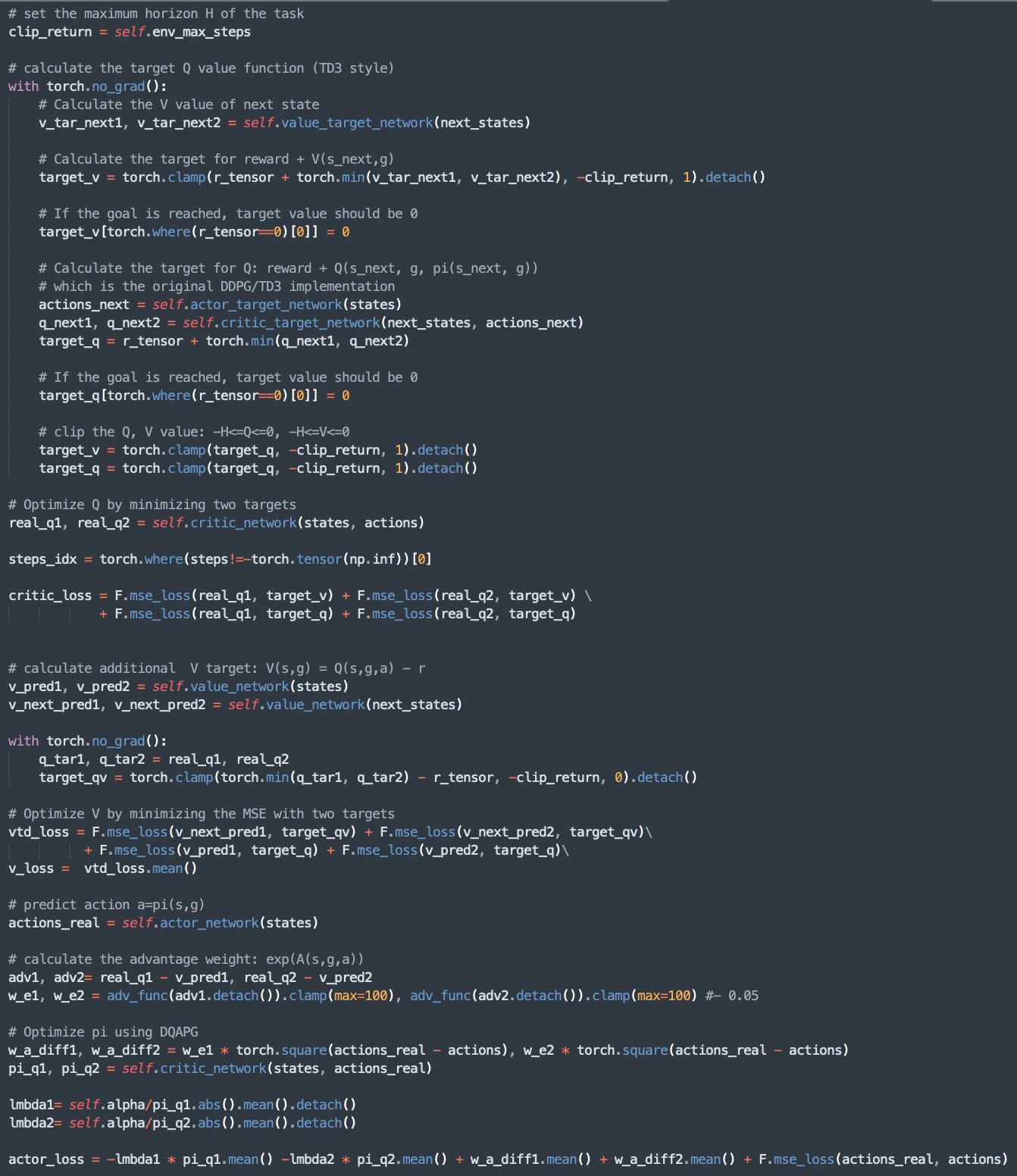
Figure 9: Core code of DQAPG.

Algorithm 3 Offline goal-conditioned Deterministic Q-Advantage policy gradient

Given offline dataset $D$, Initialize policy $\pi_{\psi}$, Q-functions $\{Q_{\theta 1},Q_{\theta 2}\}$, target Q-functions $\{Q_{\theta 1}^{tar},Q_{\theta 2}^{tar}\}$, V-functions $\{V_{\omega_{1}},V_{\omega_{2}}\}$, target V-functions $\{V_{\omega_{1}}^{tar},V_{\omega_{2}}^{tar}\}$. Denote the task’s maximum horizon as $H$, reward function as $R(\phi(s),g)$, and $\phi(s)$ maps state $s$ to goal $g$, target network update step as $h$;

1:  for i in range(epochs) do

2:     // Goal-swapping augmented experience replay

3:     Sample goal-conditioned transitions $\zeta_{i}=\{g,s_{t},a_{t},r_{t},s_{t+1}\}\sim D$:

4:     Hindsight relabel half of the batch using future goals: $\zeta_{i}=\{(\phi(s_{i}),s_{t},a_{t},R(\phi(s_{i}),s_{t}),s_{t+1}),t\leq i\leq H\}\sim D$.

5:     Sample random goals: $g_{rand}\sim D$.

6:     Generate $\tau_{rand}$ by replacing $g$ with $g_{rand}$ in $\zeta$: $\zeta_{aug}=\{(g_{rand},s_{t},a_{t},R(g_{rand},s_{t}),s_{t+1})\}\sim D$.

7:     Return $\zeta$ and $\zeta_{aug}$ for DQAPG optimization.

8:      

9:     // Value function optimization

10:     Compute $Q$ targets:

$$y_{q}(s,g,a)=r+(1-d)\underset{i=1,2}{\min}V_{\omega_{i}}^{tar}(s^{\prime},g)$$

11:     Optimize $Q$ by minimizing $\operatorname*{MSE}$ loss:

$$\underset{\theta_{i},i=1,2}{\operatorname*{arg\,min}}\operatorname*{MSE}(Q_{\theta_{i}}(s,g,a),y_{q})$$

12:     Compute $V$ targets:

$$y_{v}(s,g,a)=r+(1-d)\underset{i=1,2}{\min}Q_{\theta_{i}}^{tar}(s^{\prime},g,\pi_{\psi}(s^{\prime},g))$$

13:     Optimize $V$ by minimizing $\operatorname*{MSE}$ loss:

$$\underset{\omega_{i},i=1,2}{\operatorname*{arg\,min}}\operatorname*{MSE}(V_{\omega_{i}}(s,g,a),y_{v})$$

14:     // Policy optimization

15:     Calculate the advantage weight:

$$w_{A}=\exp(A(s,g,a))=\exp(Q_{\theta_{1}}(s,g,a)-V_{\omega_{1}}(s,g))$$

16:     Clip the advantage weights:

$$w_{A}=\min(w_{A},100)$$

17:     Policy optimization by deterministic policy gradient and advantage weighted regression:

$$\underset{\psi}{\operatorname*{arg\,min}}(-\lambda Q_{\theta 1}(s,g,\psi(s,g))+w_{e}\cdot\operatorname*{MSE}(\pi_{\psi}(s,g),a)),\quad\lambda=\frac{1}{\frac{1}{N}\sum_{s_{i},g,a_{i}}|Q(s_{i},g,a_{i})|}$$

18:     // Update the delayed target networks

19:     if $i$ mod $h=0$:

$$\omega_{i}^{tar}\leftarrow\rho\omega_{i}^{tar}+(1-\rho)\omega_{i},\quad i=1,2$$

$$\theta_{i}^{tar}\leftarrow\rho\theta_{i}^{tar}+(1-\rho)\theta_{i},\quad i=1,2$$

($\rho$ here is the polyak averaging weight).

20:  end for

References

- Andrychowicz et al. (2017) Andrychowicz, M., Wolski, F., Ray, A., Schneider, J., Fong, R., Welinder, P., McGrew, B., Tobin, J., Pieter Abbeel, O., and Zaremba, W. Hindsight experience replay. Advances in neural information processing systems, 30, 2017.
- Brandfonbrener et al. (2021) Brandfonbrener, D., Whitney, W., Ranganath, R., and Bruna, J. Offline rl without off-policy evaluation. Advances in Neural Information Processing Systems, 34:4933–4946, 2021.
- Brunke et al. (2022) Brunke, L., Greeff, M., Hall, A. W., Yuan, Z., Zhou, S., Panerati, J., and Schoellig, A. P. Safe learning in robotics: From learning-based control to safe reinforcement learning. Annual Review of Control, Robotics, and Autonomous Systems, 5:411–444, 2022.
- Chane-Sane et al. (2021) Chane-Sane, E., Schmid, C., and Laptev, I. Goal-conditioned reinforcement learning with imagined subgoals. In International Conference on Machine Learning, pp. 1430–1440. PMLR, 2021.
- Chebotar et al. (2021) Chebotar, Y., Hausman, K., Lu, Y., Xiao, T., Kalashnikov, D., Varley, J., Irpan, A., Eysenbach, B., Julian, R., Finn, C., et al. Actionable models: Unsupervised offline reinforcement learning of robotic skills. arXiv preprint arXiv:2104.07749, 2021.
- Frazier & Riedl (2019) Frazier, S. and Riedl, M. Improving deep reinforcement learning in minecraft with action advice. In Proceedings of the AAAI conference on artificial intelligence and interactive digital entertainment, volume 15, pp. 146–152, 2019.
- Fu et al. (2021) Fu, J., Kumar, A., Nachum, O., Tucker, G., and Levine, S. D4{rl}: Datasets for deep data-driven reinforcement learning, 2021. URL https://openreview.net/forum?id=px0-N3_KjA.
- Fujimoto & Gu (2021) Fujimoto, S. and Gu, S. S. A minimalist approach to offline reinforcement learning. Advances in neural information processing systems, 34:20132–20145, 2021.
- Fujimoto et al. (2018) Fujimoto, S., Hoof, H., and Meger, D. Addressing function approximation error in actor-critic methods. In International conference on machine learning, pp. 1587–1596. PMLR, 2018.
- Fujimoto et al. (2019a) Fujimoto, S., Conti, E., Ghavamzadeh, M., and Pineau, J. Benchmarking batch deep reinforcement learning algorithms. arXiv preprint arXiv:1910.01708, 2019a.
- Fujimoto et al. (2019b) Fujimoto, S., Meger, D., and Precup, D. Off-policy deep reinforcement learning without exploration. In International conference on machine learning, pp. 2052–2062. PMLR, 2019b.
- Ghosh et al. (2019) Ghosh, D., Gupta, A., Reddy, A., Fu, J., Devin, C., Eysenbach, B., and Levine, S. Learning to reach goals via iterated supervised learning. arXiv preprint arXiv:1912.06088, 2019.
- Kostrikov et al. (2021a) Kostrikov, I., Fergus, R., Tompson, J., and Nachum, O. Offline reinforcement learning with fisher divergence critic regularization. In International Conference on Machine Learning, pp. 5774–5783. PMLR, 2021a.
- Kostrikov et al. (2021b) Kostrikov, I., Nair, A., and Levine, S. Offline reinforcement learning with implicit q-learning. arXiv preprint arXiv:2110.06169, 2021b.
- Kumar et al. (2019) Kumar, A., Fu, J., Soh, M., Tucker, G., and Levine, S. Stabilizing off-policy q-learning via bootstrapping error reduction. Advances in Neural Information Processing Systems, 32, 2019.
- Kumar et al. (2020) Kumar, A., Zhou, A., Tucker, G., and Levine, S. Conservative q-learning for offline reinforcement learning. Advances in Neural Information Processing Systems, 33:1179–1191, 2020.
- LeCun et al. (2015) LeCun, Y., Bengio, Y., and Hinton, G. Deep learning. nature, 521(7553):436–444, 2015.
- Levine et al. (2020) Levine, S., Kumar, A., Tucker, G., and Fu, J. Offline reinforcement learning: Tutorial, review, and perspectives on open problems. arXiv preprint arXiv:2005.01643, 2020.
- Liu et al. (2022a) Liu, B., Feng, Y., Liu, Q., and Stone, P. Metric residual networks for sample efficient goal-conditioned reinforcement learning. arXiv preprint arXiv:2208.08133, 2022a.
- Liu et al. (2022b) Liu, M., Zhu, M., and Zhang, W. Goal-conditioned reinforcement learning: Problems and solutions. arXiv preprint arXiv:2201.08299, 2022b.
- Ma et al. (2021) Ma, X., Yang, Y., Hu, H., Liu, Q., Yang, J., Zhang, C., Zhao, Q., and Liang, B. Offline reinforcement learning with value-based episodic memory. arXiv preprint arXiv:2110.09796, 2021.
- Ma et al. (2022) Ma, Y. J., Yan, J., Jayaraman, D., and Bastani, O. Offline goal-conditioned reinforcement learning via $f$-advantage regression. In Oh, A. H., Agarwal, A., Belgrave, D., and Cho, K. (eds.), Advances in Neural Information Processing Systems, 2022. URL https://openreview.net/forum?id=_h29VprPHD.
- Mao et al. (2022) Mao, W., Yang, L., Zhang, K., and Basar, T. On improving model-free algorithms for decentralized multi-agent reinforcement learning. In International Conference on Machine Learning, pp. 15007–15049. PMLR, 2022.
- Mnih et al. (2013) Mnih, V., Kavukcuoglu, K., Silver, D., Graves, A., Antonoglou, I., Wierstra, D., and Riedmiller, M. Playing atari with deep reinforcement learning. arXiv preprint arXiv:1312.5602, 2013.
- Nair et al. (2020) Nair, A., Gupta, A., Dalal, M., and Levine, S. Awac: Accelerating online reinforcement learning with offline datasets. arXiv preprint arXiv:2006.09359, 2020.
- Nguyen & La (2019) Nguyen, H. and La, H. Review of deep reinforcement learning for robot manipulation. In 2019 Third IEEE International Conference on Robotic Computing (IRC), pp. 590–595. IEEE, 2019.
- Peng et al. (2020) Peng, X. B., Kumar, A., Zhang, G., and Levine, S. Advantage weighted regression: Simple and scalable off-policy reinforcement learning, 2020. URL https://openreview.net/forum?id=H1gdF34FvS.
- Peters & Schaal (2007) Peters, J. and Schaal, S. Reinforcement learning by reward-weighted regression for operational space control. In Proceedings of the 24th international conference on Machine learning, pp. 745–750, 2007.
- Plappert et al. (2018) Plappert, M., Andrychowicz, M., Ray, A., McGrew, B., Baker, B., Powell, G., Schneider, J., Tobin, J., Chociej, M., Welinder, P., et al. Multi-goal reinforcement learning: Challenging robotics environments and request for research. arXiv preprint arXiv:1802.09464, 2018.
- Prudencio et al. (2022) Prudencio, R. F., Maximo, M. R., and Colombini, E. L. A survey on offline reinforcement learning: Taxonomy, review, and open problems. arXiv preprint arXiv:2203.01387, 2022.
- Silver et al. (2014) Silver, D., Lever, G., Heess, N., Degris, T., Wierstra, D., and Riedmiller, M. Deterministic policy gradient algorithms. In International conference on machine learning, pp. 387–395. PMLR, 2014.
- Sutton & Barto (2018) Sutton, R. S. and Barto, A. G. Reinforcement learning: An introduction. MIT press, 2018.
- Wang et al. (2020) Wang, Z., Novikov, A., Zolna, K., Merel, J. S., Springenberg, J. T., Reed, S. E., Shahriari, B., Siegel, N., Gulcehre, C., Heess, N., et al. Critic regularized regression. Advances in Neural Information Processing Systems, 33:7768–7778, 2020.
- Wu et al. (2019) Wu, Y., Tucker, G., and Nachum, O. Behavior regularized offline reinforcement learning. arXiv preprint arXiv:1911.11361, 2019.
- Yang et al. (2022) Yang, R., Lu, Y., Li, W., Sun, H., Fang, M., Du, Y., Li, X., Han, L., and Zhang, C. Rethinking goal-conditioned supervised learning and its connection to offline rl. arXiv preprint arXiv:2202.04478, 2022.