Realizing temporal graphs from fastest travel times

Abstract

In this paper we initiate the study of the temporal graph realization problem with respect to the fastest path durations among its vertices, while we focus on periodic temporal graphs. Given an $n\times n$ matrix $D$ and a $\Delta\in\mathbb{N}$, the goal is to construct a $\Delta$-periodic temporal graph with $n$ vertices such that the duration of a fastest path from $v_{i}$ to $v_{j}$ is equal to $D_{i,j}$, or to decide that such a temporal graph does not exist. The variations of the problem on static graphs has been well studied and understood since the 1960’s, and this area of research remains active until nowadays.

As it turns out, the periodic temporal graph realization problem has a very different computational complexity behavior than its static (i.e. non-temporal) counterpart. First we show that the problem is NP-hard in general, but polynomial-time solvable if the so-called underlying graph is a tree or a cycle. Building upon those results, we investigate its parameterized computational complexity with respect to structural parameters of the underlying static graph which measure the “tree-likeness”. For those parameters, we essentially give a tight classification between parameters that allow for tractability (in the FPT sense) and parameters that presumably do not. We show that our problem is W[1]-hard when parameterized by the feedback vertex number of the underlying graph, while we show that it is in FPT when parameterized by the feedback edge number of the underlying graph.

1 Introduction

The graph realization problem with respect to a graph property $\mathcal{P}$ is to find a graph that satisfies property $\mathcal{P}$, or to decide that no such graph exists. The motivation for graph realization problems stems both from “verification” and from network design applications in engineering. In verification applications, given the outcomes of some experimental measurements (resp. some computations) on a network, the aim is to (re)construct an input network which complies with them. If such a reconstruction is not possible, this proves that the measurements are incorrect or implausible (resp. that the algorithm which made the computations is incorrectly implemented). One example of a graph realization (or reconstruction) problem is the recognition of probe interval graphs, in the context of the physical mapping of DNA, see [50, 49] and [35, Chapter 4]. In network design applications, the goal is to design network topologies having a desired property [4, 37]. Analyzing the computational complexity of the graph realization problems for various natural and fundamental graph properties $\mathcal{P}$ requires a deep understanding of these properties. Among the most studied such parameters for graph realization are constraints on the distances between vertices [8, 7, 40, 16, 10, 17], on the vertex degrees [34, 36, 39, 6, 22], on the eccentricities [5, 41, 9, 48], and on connectivity [33, 28, 15, 29, 30, 36], among others.

In the simplest version of a graph realization problem with respect to vertex distances, we are given a symmetric $n\times n$ matrix $D$ and we are looking for an $n$-vertex undirected and unweighted graph $G$ such that $D_{i,j}$ equals the distance between vertices $v_{i}$ and $v_{j}$ in $G$. This problem can be trivially solved in polynomial time in two steps [40]: First, we build the graph $G=(V,E)$ such that $v_{i}v_{j}\in E$ if and only if $D_{i,j}=1$. Second, from this graph $G$ we compute the matrix $D_{G}$ which captures the shortest distances for all pairs of vertices. If $D_{G}=D$ then $G$ is the desired graph, otherwise there is no graph having $D$ as its distance matrix. Non-trivial variations of this problem have been extensively studied, such as for weighted graphs [40, 56], as well as for cases where the realizing graph has to belong to a specific graph family [40, 7]. Other variations of the problem include the cases where every entry of the input matrix $D$ may contain a range of consecutive permissible values [7, 57, 60], or even an arbitrary set of acceptable values [8] for the distance between the corresponding two vertices.

In this paper we make the first attempt to understand the complexity of the graph realization problem with respect to vertex distances in the context of temporal graphs, i.e. of graphs whose topology changes over time.

Definition 1.1 (temporal graph [42]).

A temporal graph is a pair $(G,\lambda)$, where $G=(V,E)$ is an underlying (static) graph and $\lambda:E\rightarrow 2^{\mathbb{N}}$ is a time-labeling function which assigns to every edge of $G$ a set of discrete time-labels.

Here, whenever $t\in\lambda(e)$, we say that the edge $e$ is active or available at time $t$. In the context of temporal graphs, where the notion of vertex adjacency is time-dependent, the notions of path and distance also need to be redefined. The most natural temporal analogue of a path is that of a temporal (or time-dependent) path, which is motivated by the fact that, due to causality, entities and information in temporal graphs can “flow” only along sequences of edges whose time-labels are strictly increasing.

Definition 1.2 (fastest temporal path).

Let $(G,\lambda)$ be a temporal graph. A temporal path in $(G,\lambda)$ is a sequence $(e_{1},t_{1}),(e_{2},t_{2}),\ldots,(e_{k},t_{k})$, where $P=(e_{1},\ldots,e_{k})$ is a path in the underlying static graph $G$, $t_{i}\in\lambda(e_{i})$ for every $i=1,\ldots,k$, and $t_{1}<t_{2}<\ldots<t_{k}$. The duration of this temporal path is $t_{k}-t_{1}+1$. A fastest temporal path from a vertex $u$ to a vertex $v$ in $(G,\lambda)$ is a temporal path from $u$ to $v$ with the smallest duration. The duration of the fastest temporal path from $u$ to $v$ is denoted by $d(u,v)$.

In this paper we consider periodic temporal graphs, i.e. temporal graphs in which the temporal availability of each edge of the underlying graph is periodic. Many natural and technological systems exhibit a periodic temporal behavior. For example, in railway networks an edge is present at a time step $t$ if and only if a train is scheduled to run on the respective rail segment at time $t$ [3]. Similarly, a satellite, which makes pre-determined periodic movements, can establish a communication link (i.e. a temporal edge) with another satellite whenever they are sufficiently close to each other; the existence of these communication links is also periodic. In a railway (resp. satellite) network, a fastest temporal path from $u$ to $v$ represents the fastest railway connection between two stations (resp. the quickest communication delay between two moving satellites). Furthermore, periodicity appears also in (the otherwise quite complex) social networks which describe the dynamics of people meeting [47, 58], as every person individually follows mostly a daily routine [3].

Although periodic temporal graphs have already been studied (see [13, Class 8] and [3, 24, 55, 54]), we make here the first attempt to understand the complexity of a graph realization problem in the context of temporal graphs. Therefore, we focus in this paper on the most fundamental case, where all edges have the same period $\Delta$ (while in the more general case, each edge $e$ in the underlying graph has a period $\Delta_{e}$). As it turns out, the periodic temporal graph realization problem with respect to a given $n\times n$ matrix $D$ of the fastest duration times has a very different computational complexity behavior than the classic graph realization problem with respect to shortest path distances in static graphs.

Formally, let $G=(V,E)$ and $\Delta\in\mathbb{N}$, and let $\lambda:E\rightarrow\{1,2,\ldots,\Delta\}$ be an edge-labeling function that assigns to every edge of $G$ exactly one of the labels from $\{1,\ldots,\Delta\}$. Then we denote by $(G,\lambda,\Delta)$ the $\Delta$-periodic temporal graph $(G,L)$, where for every edge $e\in E$ we have $L(e)=\{i\Delta+x:i\geq 0,x\in\lambda(e)\}$. In this case we call $\lambda$ a $\Delta$-periodic labeling of $G$. When it is clear from the context, we drop $\Delta$ form the notation and we denote the ($\Delta$-periodic) temporal graph by $(G,\lambda)$. Given a duration matrix $D$, it is easy to observe that similar to the static case, if $D_{i,j}=1$, then $v_{i}$ and $v_{j}$ must be connected by an edge. We call the graph defined by those edges as the underlying graph of $D$.

Our contribution.

We initiate the study of naturally motivated graph realization problems in the temporal setting. Our target is not to model unreliable communication, but instead to verify that particular measurements regarding fastest temporal paths in a periodic temporal graph are plausible (i.e. “realizable”). To this end, we introduce and investigate the following problem, capturing the setting described above:

Periodic Temporal Graph Realization (Periodic TGR)
Input: An $n\times n$ matrix $D$, a positive integer $\Delta$. Question: Does there exist a graph $G=(V,E)$ with vertices $\{v_{1},\ldots,v_{n}\}$ and a $\Delta$-periodic labeling $\lambda:E\rightarrow\{1,2,\ldots,\Delta\}$ such that, for every $i,j$, the duration of the fastest temporal path from $v_{i}$ to $v_{j}$ in the $\Delta$-periodic temporal graph $(G,\lambda,\Delta)$ is $D_{i,j}$?

We focus on exact algorithms. We start with showing NP-hardness of the problem (Theorem 2.1), even if $\Delta$ is a small constant. To establish a baseline for tractability, we show that Periodic TGR is polynomial-time solvable if the underlying graph is a tree (Theorem 3.6).

Building upon these initial results, we explore the possibilities to generalize our polynomial-time algorithm using the distance-from-triviality parameterization paradigm [26, 38]. That is, we investigate the parameterized computational complexity of Periodic TGR with respect to structural parameters of the underlying graph that measure its “tree-likeness”.

We obtain the following results. We show that Periodic TGR is W[1]-hard when parameterized by the feedback vertex number of the underlying graph (Theorem 2.3). To this end, we first give a reduction from Multicolored Clique parameterized by the number of colors [25] to a variant of Periodic TGR where the period $\Delta$ is infinite, that is, when the labeling is non-periodic. We use a special gadget (the “infinity” gadget) which allows us to transfer the result to a finite period $\Delta$. The latter construction is independent from the particular reduction we use, and can hence be treated as a reduction from the non-periodic to the periodic setting. Note that our parameterized hardness result rule out fixed-parameter tractability for several popular graph parameters such as treewidth and arboricity.

We complement this result by showing that the problem is fixed-parameter tractable (FPT) with respect to the feedback edge number $k$ of the underlying graph (Theorem 3.8), a parameter that is larger than the feedback vertex number. Our FPT algorithm works as follows on a high level. First we distinguish $O(k)$ vertices which we call “interesting vertices”. Then, we guess the fastest temporal paths for each pair of these interesting vertices; as we prove, the number of choices we have for all these guesses is upper bounded by a function of $k$. Then we also make several further guesses (again using a bounded number of choices), which altogether leads us to specify a small (i.e. bounded by a function of $k$) number of different configurations for the fastest paths between all pairs of vertices. For each of these configurations, we must then make sure that the labels of our solution will not allow any other temporal path from a vertex $v_{i}$ to a vertex $v_{j}$ have a strictly smaller duration than $D_{i,j}$. This naturally leads us to build one Integer Linear Program (ILP) for each of these configurations. We manage to formulate all these ILPs by having a number of variables that is upper-bounded by a function of $k$. Finally we use Lenstra’s Theorem [46] to solve each of these ILPs in FPT time. At the end, our initial instance is a Yes-instance if and only if at least one of these ILPs is feasible.

The above results provide a fairly complete picture of the parameterized computational complexity of Periodic TGR with respect to structural parameters of the underlying graph which measure “tree-likeness”. To obtain our results, we prove several properties of fastest temporal paths, which may be of independent interest.

Due to space constraints, proofs of results marked with $\star$ are (partially) deferred to the Appendix.

Related work.

Graph realization problems on static graphs have been studied since the 1960s. We provide an overview of the literature in the introduction. To the best of our knowledge, we are the first to consider graph realization problems in the temporal setting. However, many other connectivity-related problems have been studied in the temporal setting [52, 2, 19, 53, 43, 18, 23, 27, 62, 12, 32], most of which are much more complex and computationally harder than their non-temporal counterparts, and some of which do not even have a non-temporal counterpart.

There are some problem settings that share similarities with ours, which we discuss now in more detail.

Several problems have been studied where the goal is to assign labels to (sets of) edges of a given static graph in order to achieve certain connectivity-related properties [44, 51, 1, 20]. The main difference to our problem setting is that in the mentioned works, the input is a graph and the sought labeling is not periodic. Furthermore, the investigated properties are temporal connectivity among all vertices [44, 51, 1], temporal connectivity among a subset of vertices [44], or reducing reachability among the vertices [20]. In all these cases, the duration of the temporal paths has not been considered.

Finally, there are many models for dynamic networks in the context of distributed computing [45]. These models have some similarity to temporal graphs, in the sense that in both cases the edges appear and disappear over time. However, there are notable differences. For example, one important assumption in the distributed setting can be that the edge changes are adversarial or random (while obeying some constraints such as connectivity), and therefore they are not necessarily known in advance [45].

Preliminaries and notation.

We already introduced the most central notion and concepts. There are some additional definitions we need, to present our proofs and results which we give in the following.

An interval in $\mathbb{N}$ from $a$ to $b$ is denoted by $[a,b]=\{i\in\mathbb{N}:a\leq i\leq b\}$; similarly, $[a]=[1,a]$. An undirected graph $G=(V,E)$ consists of a set $V$ of vertices and a set $E\subseteq V\times V$ of edges. For a graph $G$, we also denote by $V(G)$ and $E(G)$ the vertex and edge set of $G$, respectively. We denote an edge $e\in E$ between vertices $u,v\in V$ as a set $e=\{u,v\}$. For the sake of simplicity of the representation, an edge $e$ is sometimes also denoted by $uv$. A path $P$ in $G$ is a subgraph of $G$ with vertex set $V(P)=\{v_{1},\dots,v_{k}\}$ and edge set $E(P)=\{\{v_{i},v_{i+1}\}:1\leq i<k\}$ (we often represent path $P$ by the tuple $(v_{1},v_{2},\dots,v_{k})$).

Let $v_{1},v_{2},\ldots,v_{n}$ be the $n$ vertices of the graph $G$. For simplicity of the presentation –and with a slight abuse of notation– we refer during the paper to the entry $D_{i,j}$ of the matrix $D$ as $D_{a,b}$, where $a=v_{i}$ and $b=v_{j}$. That is, we put as indices of the matrix $D$ the corresponding vertices of $G$ whenever it is clear from the context. Many times we also refer to a path $P=(u=v_{1},v_{2},\dots,v_{p}=v)$ from $u$ to $v$ in $G$, as a temporal path in $(G,\lambda,\Delta)$, where we actually mean that $(P,\lambda,\Delta)$ is a temporal path with $P$ as its underlying (static) path.

We remark that a fastest path between two vertices in a temporal graph can be computed in polynomial time [11, 61]. Hence, given a $\Delta$-periodic temporal graph $(G,\lambda,\Delta)$, we can compute in polynomial-time the matrix $D$ which consists of durations of fastest temporal paths among all pairs of vertices in $(G,\lambda,\Delta)$.

Organization of the paper.

In Section 2 we present our hardness results, first the NP-hardness in Section 2.1 and then the parameterized hardness in Section 2.2. In Section 3 we present our algorithmic results. First we give in Section 3.3 a polynomial-time algorithm for the case where the underlying graph is a tree. In Section 3.2 we generalize this and present our FPT result, which is the main result in the paper. In Section 3.3 we provide a simple polynomial-time algorithm for the case where the underlying graph is a cycle. Finally, we conclude in Section 4 and discuss some future work directions.

2 Hardness results for Periodic TGR

In this section we present our main computational hardness results. In Section 2.1 we show that Periodic TGR is NP-hard even for constant $\Delta$. In Section 2.2 we investigate the parameterized computational hardness of Periodic TGR with respect to structural parameters of the underlying graph. We show that Periodic TGR is W[1]-hard when parameterized by the feedback vertex number of the underlying graph.

2.1 NP-hardness of Periodic TGR

In this section we prove that in general it is NP-hard to determine a $\Delta$-periodic temporal graph $(G,\lambda)$ respecting a duration matrix $D$, even if $\Delta$ is a small constant.

Theorem 2.1.

Periodic Temporal Graph Realization is NP-hard for all $\Delta\geq 3$.

Proof 2.2.

We present a polynomial-time reduction from the NP-hard problem NAE 3-SAT [59]. Here we are given a formula $\phi$ that is a conjunction of so-called NAE (not-all-equal) clauses, where each clause contains exactly 3 literals (with three distinct variables). A NAE clause evaluates to true if and only if not all of its literals are equal, that is, at least one literal evaluates to true and at least one literal evaluates to false. We are asked whether $\phi$ admits a satisfying assignment.

Given an instance $\phi$ of NAE 3-SAT, we construct an instance $(D,\Delta)$ of Periodic TGR as follows.

We start by describing the vertex set of the underlying graph $G$ of $D$.

• For each variable $x_{i}$ in $\phi$, we create three variable vertices $x_{i},x_{i}^{T},x_{i}^{F}$.

• For each clause $c$ in $\phi$, we create one clause vertex $c$.

• We add one additional super vertex $v$.

Next, we describe the edge set of $G$.

• For each variable $x_{i}$ in $\phi$ we add the following five edges: $x_{i}x_{i}^{T},x_{i}x_{i}^{F},x_{i}^{T}x_{i}^{F},x_{i}^{T}v$ and $x_{i}^{F}v$.

• For each pair of variables $x_{i},x_{j}$ in $\phi$ with $i\neq j$ we add the following four edges: $x_{i}^{T}x_{j}^{T},x_{i}^{T}x_{j}^{F},x_{i}^{F}x_{j}^{T}$ and $x_{i}^{F}x_{j}^{F}$.

• For each clause $c$ in $\phi$ we add one edge for each literal. Let $x_{i}$ appear in $c$. If $x_{i}$ appears non-negated in $c$ we add edge $cx_{i}^{T}$. If $x_{i}$ appears negated in $c$ we add edge $cx_{i}^{F}$.

This finishes the construction of $G$. For an illustration see Figure 1.

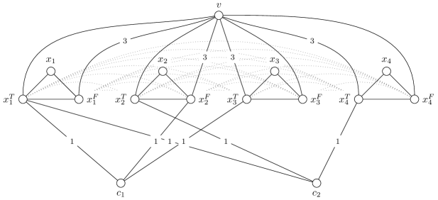
Figure 1: Illustration of the temporal graph $(G,\lambda)$ from the NP-hardness reduction, where the NAE 3-SAT formula $\phi$ is of form $\phi=\text{NAE}(x_{1},\overline{x}_{2},x_{3})\wedge\text{NAE}(x_{1},x_{2},x_{4})$. To improve the readability, we draw edges between vertices $x_{i}^{T}$ and $x_{j}^{F}$ (where $i\neq j$) with gray dotted lines. Presented is the labeling of $G$ corresponding to the assignment $x_{1}=x_{2}=\textsc{true}$ and $x_{3},x_{4}=\textsc{false}$, where all unlabeled edges get the label $2$.

We set $\Delta$ to some constant larger than two, that is, $\Delta\geq 3$. Next, we specify the durations in the matrix $D$ between all vertex pairs. For the sake of simplicity we write $D_{u,v}$ as $d(u,v)$, where $u,v$ are two vertices of $G$. We start by setting the value of $d(u,v)=1$ where $u$ and $v$ are two adjacent vertices in $G$.

• For each variable $x_{i}$ in $\phi$ and the super vertex $v$ we specify the following durations: $d(x_{i},v)=2$ and $d(v,x_{i})=\Delta$.

• For each clause $c$ in $\phi$ and the super vertex $v$ we specify the following durations: $d(c,v)=2$ and $d(v,c)=\Delta-1$.

• Let $x_{i}$ be a variable that appears in clause $c$, then we specify the following durations: $d(c,x_{i})=2$ and $d(x_{i},c)=\Delta$. If $x_{i}$ appears non-negated in $c$ we specify the following durations: $d(c,x_{i}^{F})=2$ and $d(x_{i}^{F},c)=\Delta$. If $x_{i}$ appears negated in $c$ we specify the following duratios: $d(c,x_{i}^{T})=2$ and $d(x_{i}^{T},c)=\Delta$.

• Let $x_{i}$ be a variable that does not appear in clause $c$, then we specify the following duratios: $d(x_{i},c)=2\Delta$, $d(c,x_{i})=\Delta+2$ and $d(c,x_{i}^{T})=d(c,x_{i}^{F})=2$, $d(x_{i}^{T},c)=d(x_{i}^{F},c)=\Delta$.

• For each pair of variables $x_{i}\neq x_{j}$ in $\phi$ we specify the following duratios: $d(x_{i},x_{j})=2\Delta+1$ and $d(x_{i},x_{j}^{T})=d(x_{i},x_{j}^{F})=\Delta+1$.

• For each pair of clauses $c_{i}\neq c_{j}$ in $\phi$ we specify the following duratios: $d(c_{i},c_{j})=\Delta+1$.

This finishes the construction of the instance $(D,\Delta)$ of Periodic TGR  which can clearly be done in polynomial time. In the remainder we show that $(D,\Delta)$ is a Yes-instance of Periodic TGR if and only if NAE 3-SAT formula $\phi$ is satisfiable.

$(\Rightarrow)$: Assume the constructed instance $(D,\Delta)$ of Periodic TGR is a Yes-instance. Then there exist a label $\lambda(e)$ for each edge $e\in E(G)$ such that for each vertex pair $u,w$ in the temporal graph $(G,\lambda,\Delta)$ we have that a fastest temporal path from $u$ to $w$ is of duration $d(u,w)$.

We construct a satisfying assignment for $\phi$ as follows. For each variable $x_{i}$, if $\lambda(x_{i}x_{i}^{T})=\lambda(x_{i}^{T}v)$, then we set $x_{i}$ to true, otherwise we set $x_{i}$ to false.

To show that this yields a satisfying assignment, we need to prove some properties of the labeling $\lambda$. First, observe that adding an integer $t$ to all time labels does not change the duration of any temporal paths. Second, observe that if for two vertices $u,w$ we have that $d(u,w)$ equals the distance between $u$ and $w$ in $G$ (i. e., the duration of the fastest temporal path from $u$ to $w$ equals the distance of the shortest path between $u$ and $w$), then there is a shortest path $P$ from $u$ to $w$ in $G$ such that the labeling $\lambda$ assigns consecutive time labels to the edges of $P$.

Let $\lambda(x_{i}x_{i}^{T})=t$ and $\lambda(x_{i}x_{i}^{F})=t^{\prime}$, for an arbitrary variable $x_{i}$. If both $\lambda(x_{i}^{T}v)\neq t+1$ and $\lambda(x_{i}^{F}v)\neq t^{\prime}+1$, then $d(x_{i},v)>2$, which is a contradiction. Thus, for every variable $x_{i}$, we have that $\lambda(x_{i}^{T}v)=t+1$ or $\lambda(x_{i}^{F}v)=t^{\prime}+1$ (or both). In particular, this means that if $\lambda(x_{i}x_{i}^{F})=\lambda(x_{i}^{F}v)$, then we set $x_{i}$ to false, since in this case $\lambda(x_{i}x_{i}^{T})\neq\lambda(x_{i}^{T}v)$.

Now assume for a contradiction that the described assignment is not satisfying. Then there exists a clause $c$ that is not satisfied. Suppose that $x_{1},x_{2},x_{3}$ are three variables that appear in $c$. Recall that we require $d(c,v)=2$ and $d(v,c)=\Delta-1$. The fact that $d(c,v)=2$ implies that we must have a temporal path consisting of two edges from $c$ to $v$, such that the two edges have consecutive labels. By construction of $G$ there are three candidates for such a path, one for each literal of $c$. Assume w.l.o.g. that $x_{1}$ appears in $c$ non-negated (the case of a negated appearance of $x_{1}$ is symmetrical) and that the temporal path realizing $d(c,v)=2$ goes through vertex $x_{1}^{T}$. Let us denote with $t=\lambda(x_{1}^{T}v)$. It follows that $\lambda(x_{1}^{T}c)=\lambda(x_{1}^{T}v)-1=t-1$. Furthermore, since $d(c,x_{1})=2$ we also have that $\lambda(x_{1}^{T}c)=\lambda(x_{1}x_{1}^{T})-1$. Therefore $\lambda(x_{1}x_{1}^{T})=\lambda(x_{1}^{T}v)=t$. Which implies that $x_{1}$ is set to true. Let us observe paths from $v$ to $c_{1}$. We know that $d(v,c)=\Delta-1$. The underlying path of the fastest temporal path from $v$ to $c$, that goes through $x_{1}^{T}$ is the path $P=(v,x_{1}^{T},c)$. Since $\lambda(x_{1}^{T}c)>\lambda(x_{1}^{T}v)$ we get that the duration of the temporal path $(P,\lambda)$ is equal to $d(P,\lambda)=(\Delta+t-1)-t+1=\Delta$. This implies that the fastest temporal path from $v$ to $c$ is not $(P,\lambda)$ and therefore does not pass through $x_{1}^{T}$. Since there are only two other vertices connected to $c$, we have only two other edges incident to $c$, that can be used on a fastest temporal path $v$ to $c$. Suppose now w.l.o.g. that also $x_{2}$ appears in $c$ non-negated (the case of a negated appearance of $x_{2}$ is symmetrical) and that the temporal path realizing $d(v,c)=\Delta-1$ goes through vertex $x_{2}^{T}$. Let us denote with $t^{\prime}=\lambda(x_{2}^{T}v)$. Since the fastest temporal path from $v$ to $c$ is of the duration $\Delta-1$, and the edge $x_{2}^{T}c$ is the only edge incident to vertex $c$ and edge $x_{2}^{T}v$, it follows that $\lambda(x_{2}^{T}c)\geq\lambda(x_{2}^{T}v)-2=t^{\prime}-2$. Since $d(x_{2},v)=2$ it follows that $\lambda(x_{2}x_{2}^{T})=\lambda(x_{2}^{T}v)-1=t^{\prime}-1$. Knowing this and the fact that $d(x_{2},c)=2$, we get that $\lambda(x_{2}^{T}c)$ must be equal to $t^{\prime}-2$. Therefore the fastest temporal path from $v$ to $c$ passes through edges $x_{2}^{T}v$ and $x_{2}^{T}c$. In the above we have also determined that $\lambda(x_{2}x_{2}^{T})\neq\lambda(x_{2}^{T}v)$, which implies that $x_{2}$ is set to false. But now we have that $x_{1},x_{2}$ both appear in $c$ non-negated, where one of them is true, while the other is false, which implies that the clause $c$ is satisfied, a contradiction.

$(\Leftarrow)$: Assume that $\phi$ is satisfiable. Then there exists a satisfying assignment for the variables in $\phi$.

We construct a labeling $\lambda$ as follows.

• All edges incident with a clause vertex $c$ obtain label one.

• If variable $x_{i}$ is set to true, we set $\lambda(x_{i}^{F}v)=3$.

• If variable $x_{i}$ is set to false, we set $\lambda(x_{i}^{T}v)=3$.

• We set the labels of all other edges to two.

For an example of the constructed temporal graph see Figure 1. We now verify that all duratios are realized.

• For each variable $x_{i}$ in $\phi$ we have to check that $d(x_{i},v)=2$ and $d(v,x_{i})=\Delta$.

  If $x_{i}$ is set to true, then there is a temporal path from $x_{i}$ to $v$ via $x_{i}^{F}$ of duration $2$, since $\lambda(x_{i}x_{i}^{F})=2$ and $\lambda(x_{i}^{F}v)=3$. For a temporal path from $v$ to $x_{i}$ we observe the following. The only possible labels to leave the vertex $v$ are $2$ and $3$, which take us from $v$ to $x_{j}^{T}$ or $x_{j}^{F}$ of some variable $x_{j}$. The only two edges incident to $x_{i}$ have labels $2$, therefore the fastest path from $v$ to $x_{i}$ cannot finish before the time $\Delta+2$. The fastest way to leave $v$ and enter to $x_{i}$ would then be to leave $v$ at edge $x_{i}^{F}v$ with label $3$, and continue to $x_{i}$ at time $\Delta+2$, which gives us the desired duration $\Delta$.

  If $x_{i}$ is set to false, then, by similar arguing, there is a temporal path from $x_{i}$ to $v$ via $x_{i}^{T}$ of duration $2$, and a temporal path from $v$ to $x_{i}$, through $x_{i}^{F}$ of duration $\Delta$.

• For each clause $c$ in $\phi$ we have to check that $d(c,v)=2$ and $d(v,c)=\Delta-1$:

  Suppose $x_{i},x_{j},x_{k}$ appear in $c$. Since we have a satisfying assignment at least one of the literals in $c$ is set to true and at least one to false. Suppose $x_{i}$ is the variable of the literal that is true in $c$, and $x_{j}$ is the variable of the literal that is false in $c$. Let $x_{i}$ appear non-negated in $c$ and is therefore set to true (the case when $x_{i}$ appears negated in $c$ and is set to false is symmetric). Then there is a temporal path from $c$ to $v$ through $x_{i}^{T}$ such that $\lambda(x_{i}^{T}c)=1$ and $\lambda(x_{i}^{T}v)=2$. Let $x_{j}$ appear non-negated in $c$ and is therefore set to false (the case when $x_{j}$ appears negated in $c$ and is set to true is symmetric). Then there is a temporal path from $v$ to $c$ through $x_{j}^{T}$ such that $\lambda(x_{j}^{T}v)=3$ and $\lambda(x_{j}^{T}c)=1$, which results in a temporal path from $v$ to $c$ of duration $\Delta-1$.

• Let $x_{i}$ be a variable that appears in clause $c$. If $x_{i}$ appears non-negated in $c$ we have to check that $d(c,x_{i})=d(c,x_{i}^{F})=2$ and $d(x_{i},c)=d(x_{i}^{F},c)=\Delta$.

  There is a temporal path from $c$ to $x_{i}$ via $x_{i}^{T}$ and also a temporal path from $c$ to $x_{i}^{F}$ via $x_{i}^{T}$ such that $\lambda(x_{i}^{T}c)=1$ and $\lambda(x_{i}x_{i}^{T})=\lambda(x_{i}^{T}x_{i}^{F})=2$, which proves the first equality. There are also the following two temporal paths, first, from $x_{i}$ to $c$ through $x_{i}^{T}$ and second, from $x_{i}^{F}$ to $c$ through $x_{i}^{T}$. Both of the temporal paths start on the edge with label $2$, as $\lambda(x_{i}x_{i}^{T})=\lambda(x_{i}^{T}x_{i}^{F})=2$ and finish on the edge with label $1$, as $\lambda(x_{i}^{T}c)=1$.

  If $x$ appears negated in $c$ we have to check that $d(c,x_{i})=d(c,x_{i}^{T})=2$ and $d(x_{i},c)=d(x_{i}^{T},c)=\Delta$.

  There is a temporal path from $c$ to $x$ via $x^{F}$ and also a temporal path from $c$ to $x^{T}$ via $x^{F}$ such that $\lambda(cx^{F})=1$ and $\lambda(xx^{F})=\lambda(x^{T}x^{F})=2$, which proves the first inequality. There are also the following two temporal paths, first, from $x_{i}$ to $c$ through $x_{i}^{F}$ and second, from $x_{i}^{T}$ to $c$ through $x_{i}^{F}$. Both of the temporal paths start on the edge with label $2$, as $\lambda(x_{i}x_{i}^{F})=\lambda(x_{i}^{T}x_{i}^{F})=2$ and finish on the edge with label $1$, as $\lambda(x_{i}^{F}c)=1$. Which proves the second equality.

• Let $x_{i}$ be a variable that does not appear in clause $c$, then we have to check that first, $d(c,x_{i}^{T})=d(c,x_{i}^{F})=2$, second, $d(x_{i}^{T},c)=d(x_{i}^{F},c)=\Delta$, third, $d(c,x_{i})=\Delta+2$, and fourth $d(x_{i},c)=2\Delta$.

  Let $x_{j}$ be a variable that appears non-negated in $c$ (the case where $x_{j}$ appears negated is symmetric). Then there is a temporal path from $c$ to $x_{i}^{T}$ via $x_{j}^{T}$ and also a temporal path from $c$ to $x_{i}^{F}$ via $x_{j}^{T}$ such that $\lambda(x_{j}^{T}c)=1$ and $\lambda(x_{j}^{T}x_{i}^{T})=\lambda(x_{j}^{T}x_{i}^{F})=2$, which proves the first equality. Using the same temporal path in the opposite direction, i. e., first the edge $x_{j}^{T}c$ and then one of the edges $x_{j}^{T}x_{i}^{F}$ or $x_{j}^{T}x_{i}^{T}$ at times $2$ and $\Delta+1$, respectively, yields the second equality. For a temporal path from $c$ to $x_{i}$ we traverse the following three edges $x_{j}^{T}c,x_{j}^{T}x_{i}^{F}$ and $x_{i}^{F}x_{i}$, with labels $1,2,2$ respectively (i. e., the path traverses them at time $1,2$ and $\Delta+2$, respectively), which proves the third equality. Now for the case of a temporal path from $x_{i}$ to $c$, we use the same three edges, but in the opposite direction, namely $x_{i}^{F}x_{i},x_{j}^{T}x_{i}^{F}$ and $x_{j}^{T}c$, again at times $2,\Delta+2,2\Delta+1$, respectively, which proves the last equality. Note that all of the above temporal paths are also the shortest possible, and since the labels of first and last edges (of these paths) are unique, it follows that we cannot find faster temporal paths.

• For each pair of variables $x_{i}\neq x_{j}$ in $\phi$ we have to check that $d(x_{i},x_{j})=2\Delta+1$ and $d(x_{i},x_{j}^{T})=d(x_{i},x_{j}^{F})=\Delta+1$.

  There is a path from $x_{i}$ to $x_{j}$ that passes first through one of the vertices $x_{i}^{T}$ or $x_{i}^{F}$, and then through one of the vertices $x_{j}^{T}$ or $x_{j}^{F}$. This temporal path is of length $3$, where all of the edges have label $2$, which proves the first equality. Now, a temporal path from $x_{i}$ to $x_{j}^{T}$ (resp. $x_{j}^{F}$), passes through one of the vertices $x_{i}^{T}$ or $x_{i}^{F}$. This path is of length two, where all of the edges have label $2$, which proves the second equality. Note that all of the above temporal paths are also the shortest possible, and since the labels of first and last edges (of these paths) are unique, it follows that we cannot find faster temporal paths.

• For each pair of clauses $c_{i}\neq c_{j}$ in $\phi$ we have to check that $d(c_{i},c_{j})=\Delta+1$.

  Let $x_{k}$ be a variable that appears non-negated in $c_{i}$ and $x_{\ell}$ the variable that appears non-negated in $c_{j}$ (all other cases are symmetric). There is a path of length three from $c_{i}$ to $c_{j}$ that passes first through vertex $x_{k}^{T}$ and then through vertex $x_{\ell}^{T}$. Therefore the temporal path from $c_{i}$ to $c_{j}$ uses the edges $x_{k}^{T}c_{i},x_{\ell}^{T}c_{j},x_{k}^{T}x_{\ell}^{T}$, with labels $1,2,1$ (at times $1,2,\delta+1$), respectively, which proves the desired equality. Note also that this is the shortest path between $c_{i}$ and $c_{j}$, and that the first and the last edge must have the label $1$, therefore it follows that this is the fastest temporal path.

Lastly, observe that the above constructed labeling $\lambda$ uses values $\{1,2,3\}\subseteq[\Delta]$, therefore $\Delta\geq 3$.

2.2 Parameterized hardness of Periodic TGR

In this section, we investigate the parameterized hardness of Periodic TGR with respect to structural parameters of the underlying graph. We show that the problem is W[1]-hard when parameterized by the feedback vertex number of the underlying graph. The feedback vertex number of a graph $G$ is the cardinality of a minimum vertex set $X\subseteq V(G)$ such that $G-X$ is a forest. The set $X$ is called a feedback vertex set. Note that, in contrast to the result of the previous section (Theorem 2.1), the reduction we use to obtain the following result does not produce instances with a constant $\Delta$.

Theorem 2.3.

Periodic Temporal Graph Realization is W[1]-hard when parameterized by the feedback vertex number of the underlying graph.

Proof 2.4.

We present a parameterized reduction from the W[1]-hard problem Multicolored Clique parameterized by the number of colors [25]. Here, given a $k$-partite graph $H=(W_{1}\uplus W_{2}\uplus\ldots\uplus W_{k},F)$, we are asked whether $H$ contains a clique of size $k$. If $w\in W_{i}$, then we say that $w$ has color $i$. W.l.o.g. we assume that $|W_{1}|=|W_{2}|=\ldots=|W_{k}|=n$ and that every vertex has at least one neighbor of every color. Furthermore, for all $i\in[k]$, we assume the vertices in $W_{i}$ are ordered in some arbitrary but fixed way, that is, $W_{i}=\{w^{i}_{1},w^{i}_{2},\ldots,w^{i}_{n}\}$. Let $F_{i,j}$ with $i<j$ denote the set of all edges between vertices from $W_{i}$ and $W_{j}$. We assume w.l.o.g. that $|F_{i,j}|=m$ for all $i<j$. Furthermore, for all $i<j$ we assume that the edges in $F_{i,j}$ are ordered in some arbitrary but fixed way, that is, $F_{i,j}=\{e^{i,j}_{1},e^{i,j}_{2},\ldots,e^{i,j}_{m}\}$.

We give a reduction to a variant of Periodic Temporal Graph Realization where the period $\Delta$ is infinite (that is, there are no periods) and we allow $D$ to have infinity entries, meaning that the two respective vertices are not temporally connected. At the end of the proof we show how to obtain the result for a finite $\Delta$ and a matrix $D$ of durations of fastest paths, that only has finite entries.

Given an instance $H$ of Multicolored Clique, we construct an instance $D$ of Periodic Temporal Graph Realization (with infinity entries and no periods) as follows. To ease the presentation, we first describe the underlying graph $G$ that is implicitly defined by the entries $D_{v,v^{\prime}}=1$, that is, the pairs of vertices $v,v^{\prime}$ that should be connected by a temporal path of duration one, meaning that there needs to be an edge connecting the two vertices. Afterwards, we describe the remaining entries of $D$. We will construct $G$ using several gadgets.

Edge selection gadget.

We first introduce an edge selection gadget $G_{i,j}$ for color combination $i,j$ with $i<j$. We start with describing the vertex set of the gadget.

• A set $X_{i,j}$ of vertices $x_{1},x_{2},\ldots,x_{m}$.

• Vertex sets $U_{1},U_{2},\ldots,U_{m}$ with $4n+1$ vertices each, that is, $U_{\ell}=\{u^{\ell}_{0},u^{\ell}_{1},u^{\ell}_{2},\ldots,u^{\ell}_{4n}\}$ for all $\ell\in[m]$.

• Two special vertices $v_{i,j}^{\star},v_{i,j}^{\star\star}$.

The gadget has the following edges.

• For all $\ell\in[m]$ we have edge $\{x_{\ell},v_{i,j}^{\star}\}$, $\{v_{i,j}^{\star},u^{\ell}_{0}\}$, and $\{u^{\ell}_{4n},v_{i,j}^{\star\star}\}$.

• For all $\ell\in[m]$ and $\ell^{\prime}\in[4n]$, we have edge $\{u^{\ell}_{\ell^{\prime}-1},u^{\ell}_{\ell^{\prime}}\}$.

Verification gadget.

For each color $i$, we introduce the following vertices. What we describe in the following will be used as a verification gadget for color $i$.

• We have one vertex $y^{i}$ and $k+1$ vertices $v^{i}_{\ell}$ for $0\leq\ell\leq k$.

• For every $\ell\in[m]$ and every $j\in[k]\setminus\{i\}$ we have $5n$ vertices $a^{i,j,\ell}_{1},a^{i,j,\ell}_{2},\ldots,a^{i,j,\ell}_{5n}$ and $5n$ vertices $b^{i,j,\ell}_{1},b^{i,j,\ell}_{2},\ldots,b^{i,j,\ell}_{5n}$.

• We have a set $\hat{U}_{i}$ of $13n+1$ vertices $\hat{u}^{i}_{1},\hat{u}^{i}_{2},\ldots,\hat{u}^{i}_{13n+1}$.

We add the following edges. We add edge $\{y^{i},v^{i}_{0}\}$. For every $\ell\in[m]$, every $j\in[k]\setminus\{i\}$, and every $\ell^{\prime}\in[5n-1]$ we add edge $\{a^{i,j,\ell}_{\ell^{\prime}},a^{i,j,\ell}_{\ell^{\prime}+1}\}$ and we add edge $\{b^{i,j,\ell}_{\ell^{\prime}},b^{i,j,\ell}_{\ell^{\prime}+1}\}$.

Let $1\leq j<i$ (skip if $i=1$), let $e_{\ell}^{j,i}\in F_{j,i}$, and let $w^{i}_{\ell^{\prime}}\in W_{i}$ be incident with $e_{\ell}^{j,i}$. Then we add edge $\{v_{j-1}^{i},a^{i,j,\ell}_{1}\}$ and we add edge $\{a^{i,j,\ell}_{5n},u^{\ell}_{\ell^{\prime}-1}\}$ between $a^{i,j,\ell}_{5n}$ and the vertex $u^{\ell}_{\ell^{\prime}-1}$ of the edge selection gadget of color combination $j,i$. Furthermore, we add edge $\{v_{j}^{i},b^{i,j,\ell}_{1}\}$ and edge $\{b^{i,j,\ell}_{5n},u^{\ell}_{\ell^{\prime}}\}$ between $b^{i,j,\ell}_{5n}$ and the vertex $u^{\ell}_{\ell^{\prime}}$ of the edge selection gadget of color combination $j,i$.

We add edge $\{v^{i}_{i-1},\hat{u}^{i}_{1}\}$ and for all $\ell\in[13n]$ we add edge $\{\hat{u}^{i}_{\ell},\hat{u}^{i}_{\ell+1}\}$. Furthermore, we add edge $\{\hat{u}^{i}_{13n+1},v^{i}_{i}\}$.

Let $i<j\leq k$ (skip if $i=k$), let $e_{\ell}^{i,j}\in F_{i,j}$, and let $w^{i}_{\ell^{\prime}}\in W_{i}$ be incident with $e_{\ell}^{i,j}$. Then we add edge $\{v_{j-1}^{i},a^{i,j,\ell}_{1}\}$ and edge $\{a^{i,j,\ell}_{5n},u^{\ell}_{3n+\ell^{\prime}-1}\}$ between $a^{i,j,\ell}_{5n}$ and the vertex $u^{\ell}_{3n+\ell^{\prime}-1}$ of the edge selection gadget of color combination $i,j$. Furthermore, we add edge $\{v_{j}^{i},b^{i,j,\ell}_{1}\}$ and edge $\{b^{i,j,\ell}_{5n},u^{\ell}_{3n+\ell^{\prime}}\}$ between $b^{i,j,\ell}_{5n}$ and the vertex $u^{\ell}_{3n+\ell^{\prime}}$ of the edge selection gadget of color combination $i,j$.

Connector gadget.

Next, we describe connector gadgets. Intuitively, these gadgets will be used to connect many vertex pairs by fast paths, which will make arguing about possible labelings in Yes-instances much easier. Connector gadgets consist of six vertices $\hat{v}_{0},\hat{v}_{0}^{\prime},\hat{v}_{1},\hat{v}_{2},\hat{v}_{3},\hat{v}_{3}^{\prime}$. Each connector gadget is associated with two sets $A,B$ with $B\subseteq A$ containing vertices of other gadgets. Let $V^{\star}$ denote the set of all vertices from all edge selection gadgets and all validation gadgets. The sets $A$ and $B$ will only play a role when defining the matrix $D$ later. Informally speaking, vertices in $A$ should reach all vertices in $V^{\star}$ quickly through the gadget, except the ones in $B$. We have the following edges.

• Edges $\{\hat{v}_{0},\hat{v}_{1}\},\{\hat{v}_{0}^{\prime},\hat{v}_{1}\},\{\hat{v}_{1},\hat{v}_{2}\},\{\hat{v}_{2},\hat{v}_{3}\},\{\hat{v}_{2},\hat{v}_{3}^{\prime}\}$.

• An edge between $\hat{v}_{1}$ and each vertex in $V^{\star}$.

• An edge between $\hat{v}_{2}$ and each vertex in $V^{\star}$.

We add two connector gadgets for each edge selection gadget and two connector gadgets for each validation gadget.

The first connector gadget for the edge selection gadget of color combination $i,j$ with $i<j$ has the following sets.

• Sets $A$ and $B$ contain all vertices in $X_{i,j}$ and vertex $v_{i,j}^{\star\star}$.

The second connector gadget for the edge selection gadget of color combination $i,j$ with $i<j$ has the following sets.

• Set $A$ contains all vertices from the edge selection gadget $G_{i,j}$ except vertices in $X_{i,j}$.

• Set $B$ is empty.

The first connector gadget for the verification gadget of color $i$ has the following sets.

• Sets $A$ and $B$ contain all vertices $v^{i}_{\ell}$ with $0\leq\ell\leq k$.

The second connector gadget for the verification gadget of color $i$ has the following sets.

• Set $A$ contains all vertices of the verification gadget except vertices $v^{i}_{\ell}$ with $0\leq\ell\leq k$.

• Set $B$ is empty.

Alignment gadget.

Lastly, we introduce an alignment gadget. It consists of one vertex $w^{\star}$ and a set of vertices $\hat{W}$ containing one vertex for each edge selection gadget, one vertex for each verification gadget, and one vertex for each connector gadget. Vertex $w^{\star}$ is connected to each vertex in $\hat{W}$. The vertex $x_{1}$ of each edge selection gadget, the vertex $y^{i}$ of each verification gadget, and the vertex $\hat{v}_{1}$ of each connector gadget are each connected to one vertex in $\hat{W}$ such that all vertices in $\hat{W}$ have degree two. Intuitively, this gadget is used to relate labels of different gadgets to each other.

Feedback vertex number.

This finished the description of the underlying graph $G$. For an illustration see Figure 2. We can observe that the vertex set containing

• vertices $v_{i,j}^{\star}$ and $v_{i,j}^{\star\star}$ of each edge selection gadget,

• vertices $v^{i}_{\ell}$ with $0\leq\ell\leq k$ of each verification gadget,

• vertices $\hat{v}_{1}$ and $\hat{v}_{2}$ of each connector gadget, and

• vertex $w^{\star}$ of the alignment gadget

forms a feedback vertex set in $G$ with size $O(k^{2})$.

Duration matrix $D$.

We proceed with describing the matrix $D$ of durations of fastest paths. For a more convenient presentation, we use the notation $d(v,v^{\prime}):=D_{v,v^{\prime}}$. For all vertices $v,v^{\prime}$ that are neighbors in $G$ we have that $d(v,v^{\prime})=1$ and $d(v^{\prime},v)=1$.

Next, consider a connector gadget consisting of vertices $\hat{v}_{0},\hat{v}_{0}^{\prime},\hat{v}_{1},\hat{v}_{2},\hat{v}_{3},\hat{v}_{3}^{\prime}$ and with sets $A$ and $B$. Informally, the connector gadget makes sure that all vertices in $A$ can reach all other vertices (of edge selection gadgets and validation gadgets) except the ones in $B$. We set the following durations. Recall that $V^{\star}$ denotes the set of all vertices from all edge selection gadgets and all validation gadgets.

• We set $d(\hat{v}_{0},\hat{v}_{2})=d(\hat{v}_{3},\hat{v}_{1})=d(\hat{v}_{2},\hat{v}_{0}^{\prime})=d(\hat{v}_{1},\hat{v}_{3}^{\prime})=2$, and $d(\hat{v}_{0},\hat{v}_{0}^{\prime})=d(\hat{v}_{3},\hat{v}_{3}^{\prime})=d(\hat{v}_{0},\hat{v}_{3}^{\prime})=d(\hat{v}_{3},\hat{v}_{0}^{\prime})=3$.

• Let $v\in A$, then we set $d(v,\hat{v}_{0}^{\prime})=3$ and $d(v,\hat{v}_{3}^{\prime})=3$.

• Let $v\in V^{\star}\setminus B$, then we set $d(\hat{v}_{0},v)=3$ and $d(\hat{v}_{3},v)=3$.

• Let $v\in A$ and $v^{\prime}\in V^{\star}\setminus B$ such that $v$ and $v^{\prime}$ are not neighbors, then we set $d(v,v^{\prime})=3$.

Now consider two connector gadgets, one with vertices $\hat{v}_{0},\hat{v}_{0}^{\prime},\hat{v}_{1},\hat{v}_{2},\hat{v}_{3},\hat{v}_{3}^{\prime}$ and with sets $A$ and $B$, and one with vertices $\hat{v}_{0}^{\prime},\hat{v}_{0}^{\prime\prime},\hat{v}_{1}^{\prime},\hat{v}_{2}^{\prime},\hat{v}_{3}^{\prime},\hat{v}_{3}^{\prime\prime}$ and with sets $A^{\prime}$ and $B^{\prime}$.

• If there is a vertex $v\in A$ with $v\notin A^{\prime}$, then we set $d(\hat{v}_{1},\hat{v}_{1}^{\prime})=3$.

• If there is a vertex $v\in A$ with $v\in A^{\prime}\setminus B^{\prime}$, then we set $d(\hat{v}_{1},\hat{v}_{2}^{\prime})=3$.

• If there is a vertex $v\in V^{\star}\setminus(A\setminus B)$ with $v\notin A^{\prime}$, then we set $d(\hat{v}_{2},\hat{v}_{1}^{\prime})=3$.

• If there is a vertex $v\in V^{\star}\setminus(A\setminus B)$ with $v\in A^{\prime}\setminus B^{\prime}$, then we set $d(\hat{v}_{2},\hat{v}_{2}^{\prime})=3$.

Next, consider the edge selection gadget for color combination $i,j$ with $i<j$.

• Let $1\leq\ell<\ell^{\prime}\leq m$. We set $d(x_{\ell},x_{\ell^{\prime}})=2n\cdot(i+j)\cdot((\ell^{\prime})^{2}-\ell^{2})+1$.

• For all $\ell\in[m]$ we set $d(x_{\ell},v_{i,j}^{\star\star})=8n+5$.

Next, consider the validation gadget for color $i$. For all $0\leq j<j^{\prime}<i$ and all $i\leq j<j^{\prime}\leq k$ we set the following.

• We set $d(v^{i}_{j},v^{i}_{j^{\prime}})=(20n+6)(j^{\prime}-j)-1$.

For all $0\leq j<i$ and all $i\leq j^{\prime}\leq k$ we set the following.

• We set $d(v^{i}_{j},v^{i}_{j^{\prime}})=(20n+6)(j^{\prime}-j)+6n-1$.

Finally, we consider the alignment gadget. Let $x_{1}$ belong to the edge selection gadget of color combination $i,j$ and let $w\in\hat{W}$ denote the neighbor of $x_{1}$ in the alignment gadget. Let $\hat{v}_{1}$ and $\hat{v}_{2}$ belong to the first connector gadget of the edge selection gadget for color combination $i,j$. Let $\hat{V}$ contain all vertices $\hat{v}_{1}$ and $\hat{v}_{2}$ belonging to the other connector gadgets (different from the first one of the edge selection gadget for color combination $i,j$).

• We set $d(w^{\star},x_{1})=(20n+6)(i+j)$.

• We set $d(w^{\star},\hat{v}_{1})=n^{9}$, $d(w,\hat{v}_{2})=n^{9}$, $d(w,\hat{v}_{1})=n^{9}-(20n+6)(i+j)+1$, and $d(w,\hat{v}_{2})=n^{9}-(20n+6)(i+j)+1$.

• For each vertex $v\in(V^{\star}\cup\hat{V})\setminus(X_{i,j}\cup\{v_{i,j}^{\star\star}\})$ we set $d(w^{\star},v)=n^{9}+2$ and $d(w,v)=n^{9}-(20n+6)(i+j)+3$.

Let $y^{i}$ belong to the verification gadget of color $i$ and let $w^{\prime}\in\hat{W}$ denote the neighbor of $y^{i}$ in the alignment gadget. Let $\hat{v}_{1}$ and $\hat{v}_{2}$ belong to the connector gadget of the verification gadget for color $i$. Let $\hat{V}$ contain all vertices $\hat{v}_{1}$ and $\hat{v}_{2}$ belonging to the other connector gadgets (different from the one of the verification gadget for color $i$). Let $V_{i}$ denote the set of all vertices of the verification gadget of color $i$.

• We set $d(w^{\star},y^{i})=n^{8}-1$, $d(w^{\prime},v^{i}_{0})=2$, and $d(w^{\star},v^{i}_{0})=n^{8}$.

• We set $d(w^{\star},\hat{v}_{1})=n^{9}$, $d(w^{\star},\hat{v}_{2})=n^{9}$, $d(w^{\prime},\hat{v}_{1})=n^{9}-n^{8}$, and $d(w^{\prime},\hat{v}_{2})=n^{9}-n^{8}$.

• For each vertex $v\in(V^{\star}\cup\hat{V})\setminus V_{i}$ we set $d(w^{\star},v)=n^{9}+1$, $d(w,v)=n^{9}-n^{8}+2$, and $d(y^{i},v)=n^{9}-n^{8}+2$.

Let $\hat{v}_{1}$ belong to some connector gadget. Then we set $d(w^{\star},\hat{v}_{1})=n^{9}$.

All fastest path durations between non-adjacent vertex pairs that are not specified above are set to infinity.

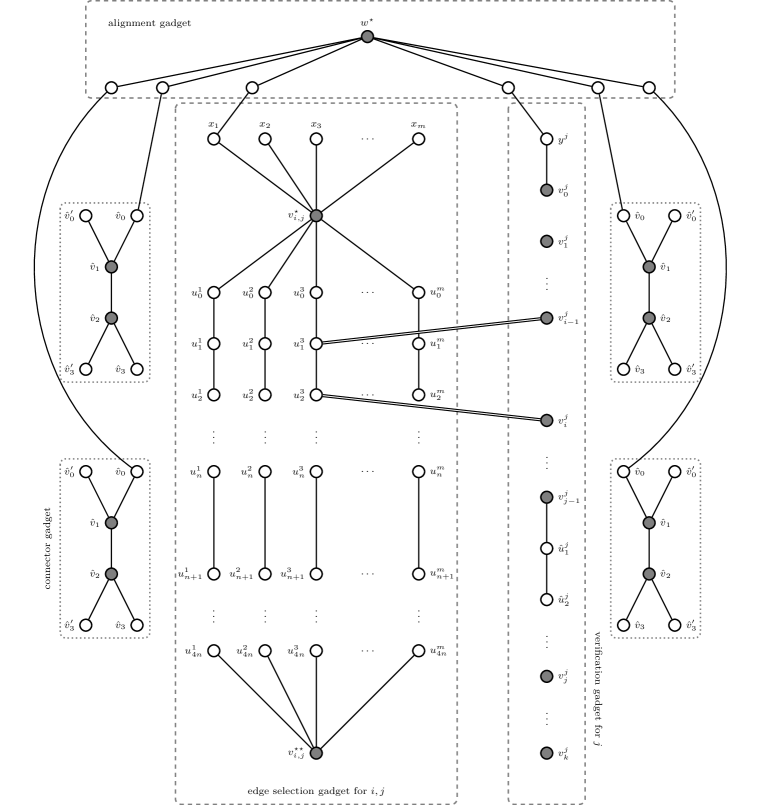
Figure 2: Illustration of part of the underlying graph $G$ and a possible labeling. Edges incident with vertices $\hat{v}_{1},\hat{v}_{2}$ of connector gadgets are omitted. Gray vertices form a feedback vertex set. The double line connections, between a vertex $v_{i-1}^{j}$ in the verification gadget, and $u_{1}^{3}$ in the edge selection gadget, and, between a vertex $u_{2}^{3}$ in the edge selection gadget, and $v_{i}^{j}$ in the verification gadget, consist of $5n$ vertices $a_{1}^{j,i,3},a_{2}^{j,i,3},\dots,a_{5n}^{j,i,3}$ and $b_{1}^{j,i,3},b_{2}^{j,i,3},\dots,b_{5n}^{j,i,3}$, respectively.

Correctness.

This finishes the construction of Periodic Temporal Graph Realization instance $D$, which can clearly be computed in polynomial time. For an illustration see Figure 2. As discussed earlier, we have that the vertex cover number of the underlying graph of the instance is in $O(k^{2})$.

In the remainder we prove that $D$ is a Yes-instance of Periodic Temporal Graph Realization if and only if the $H$ is a Yes-instance of Multicolored Clique.

$(\Rightarrow)$:

Assume $D$ is a Yes-instance of Periodic Temporal Graph Realization and let $(G,\lambda)$ be a solution. We have that the underlying graph $G$ is uniquely defined by $D$. We first prove a number of properties of $\lambda$ that we need to define a set of vertices in $H$ which we claim to be a multicolored clique.

To start, consider the alignment gadget. We can observe that all edges incident with $w^{\star}$ have the same label.

Claim 1.

For all $w\in\hat{W}$ we have that $\lambda(\{w^{\star},w\})=t$ for some $t\in\mathbb{N}$.

Assume for contradiction that there are $w,w^{\prime}\in\hat{W}$ such that $\lambda(\{w^{\star},w\})=t$ and $\lambda(\{w^{\star},w^{\prime}\})=t^{\prime}$ with $t\neq t^{\prime}$. Let w.l.o.g. $t<t^{\prime}$. Then $w$ can reach $w^{\prime}$, however we have that $d(w,w^{\prime})=\infty$, a contradiction. Claim 1 allows us to assume w.l.o.g. that all edges incident with vertex $w^{\star}$ of the alignment gadget have label $1$. From now we will assume that this is the case.

Next, we analyse the labelings of connector gadgets. We show that all edges incident with vertices of connector gadgets have labels of at least $n^{9}$ and at most $n^{9}+2$. More precisely, we show the following.

Claim 2.

Let $\hat{v}_{0},\hat{v}_{0}^{\prime},\hat{v}_{1},\hat{v}_{2},\hat{v}_{3},\hat{v}_{3}^{\prime}$ be the vertices of a connector gadget with sets $A$ and $B$. Then we have that $\lambda(\{\hat{v}_{0},\hat{v}_{1}\})=n^{9}$, $\lambda(\{\hat{v}_{0}^{\prime},\hat{v}_{1}\})=n^{9}+2$, $\lambda(\{\hat{v}_{1},\hat{v}_{2}\})=n^{9}+1$, $\lambda(\{\hat{v}_{2},\hat{v}_{3}\})=n^{9}$, and $\lambda(\{\hat{v}_{2},\hat{v}_{3}^{\prime}\})=n^{9}+2$. Furthermore, for all $v\in V^{\star}$ we have $n^{9}\leq\lambda(\{\hat{v}_{1},v\})\leq n^{9}+2$ and $n^{9}\leq\lambda(\{\hat{v}_{2},v\})\leq n^{9}+2$.

Let $w\in\hat{W}$ denote the vertex of the alignment gadget that is neighbor of $w^{\star}$ and $\hat{v}_{0}$. We have $d(w^{\star},\hat{v}_{0})=n^{9}$. It follows that $\lambda(\{w,\hat{v}_{0}\})=n^{9}$. Since $d(\hat{v}_{1},w)=\infty$ and $d(w,\hat{v}_{1})=\infty$, we have that $\lambda(\{\hat{v}_{0},\hat{v}_{1}\})=n^{9}$. Note that $\hat{v}_{1}$ is the only common neighbor of $\hat{v}_{0}$ and $\hat{v}_{2}$ and the only common neighbor of $\hat{v}_{0}$ and $\hat{v}_{0}^{\prime}$. Since $d(\hat{v}_{0},\hat{v}_{2})=2$ and $d(\hat{v}_{0},\hat{v}_{0}^{\prime})=3$ we have that $\lambda(\{\hat{v}_{1},\hat{v}_{2}\})=n^{9}+1$ and $\lambda(\{\hat{v}_{0}^{\prime},\hat{v}_{1}\})=n^{9}+2$. Similarly, we have that $\hat{v}_{2}$ is the only common neighbor of $\hat{v}_{3}$ and $\hat{v}_{1}$ and the only common neighbor of $\hat{v}_{3}$ and $\hat{v}_{3}^{\prime}$. Since $d(\hat{v}_{3},\hat{v}_{1})=2$ and $d(\hat{v}_{3},\hat{v}_{3}^{\prime})=3$ we have that $\lambda(\{\hat{v}_{2},\hat{v}_{3}\})=n^{9}$ and $\lambda(\{\hat{v}_{2},\hat{v}_{3}^{\prime}\})=n^{9}+2$.

Let $v\in V^{\star}$. Note that $d(v,\hat{v}_{0})=\infty$ and $d(v,\hat{v}_{3})=\infty$. It follows that $\lambda(\{\hat{v}_{1},v\})\geq n^{9}$ and $\lambda(\{\hat{v}_{2},v\})\geq n^{9}$. Otherwise, there would be a temporal path from $v$ to $\hat{v}_{0}$ via $\hat{v}_{1}$ or a temporal path from $v$ to $\hat{v}_{3}$ via $\hat{v}_{2}$, a contradiction. Furthermore, note that $d(\hat{v}_{0}^{\prime},v)=\infty$ and $d(\hat{v}_{3}^{\prime},v)=\infty$. It follows that $\lambda(\{\hat{v}_{1},v\})\leq n^{9}+2$ and $\lambda(\{\hat{v}_{2},v\})\leq n^{9}+2$. Otherwise, there would be a temporal path from $\hat{v}_{0}^{\prime}$ to $v$ via $\hat{v}_{1}$ or a temporal path from $\hat{v}_{3}$ to $v$ via $\hat{v}_{2}$, a contradiction.

Now we take a closer look at the edge selection gadgets. We make a number of observations that will allow us to define a set of vertices in $H$ that we claim to be a multicolored clique.

Claim 3.

For all $1\leq i<j\leq k$ and $\ell\in[m]$ we have that $\lambda(\{u^{\ell}_{4n},v_{i,j}^{\star\star}\})\leq n^{9}+2$, where $u^{\ell}_{4n}$ belongs to the edge selection gadget for $i,j$.

Consider the first connector gadget of the edge selection gadget for $i,j$ with vertices $\hat{v}_{0},\hat{v}_{0}^{\prime},\hat{v}_{1},\hat{v}_{2},\hat{v}_{3},\hat{v}_{3}^{\prime}$ and sets $A,B$. Recall that $v_{i,j}^{\star\star}\in B$ and hence we have that $d(\hat{v}_{0},v_{i,j}^{\star\star})=\infty$. Furthermore, we have that $u^{\ell}_{4n}\notin B$ and hence $d(\hat{v}_{0},u^{\ell}_{4n})=3$. By Claim 2 and the fact that $d(w^{\star},\hat{v}_{0})=n^{9}$ we have that both edges incident with $\hat{v}_{0}$ have label $n^{9}$. It follows that a fastest temporal path from $\hat{v}_{0}$ to $u^{\ell}_{4n}$ arrives at $u^{\ell}_{4n}$ at time $n^{9}+2$. Now assume for contradiction that $\lambda(\{u^{\ell}_{4n},v_{i,j}^{\star\star}\})>n^{9}+2$. Then there exists a temporal walk from $\hat{v}_{0}$ to $v_{i,j}^{\star\star}$ via $u^{\ell}_{4n}$, a contradiction to $d(\hat{v}_{0},v_{i,j}^{\star\star})=\infty$.

Claim 4.

For all $1\leq i<j\leq k$ and $\ell\in[m]$ we have that $\lambda(\{x_{\ell},v_{i,j}^{\star}\})=(i+j)\cdot(2n\ell^{2}+18n+6)$, where $x_{\ell}$ belongs to the edge selection gadget for $i,j$.

We first determine the label of $\{x_{1},v_{i,j}^{\star}\}$, where $x_{1}$ belongs to the edge selection gadget for $i,j$. Note that $x_{1}$ is connected to the alignment gadget. Let $w\in\hat{W}$ be the vertex of the alignment gadget that is a neighbor of $x_{1}$. Since $d(w^{\star},x_{1})=(20n+6)(i+j)$ we have that $\lambda(\{w,x_{1}\})=(20n+6)(i+j)$.

First, assume that $\lambda(\{x_{1},v_{i,j}^{\star}\})<(20n+6)(i+j)$. Then there is a temporal path from $v_{i,j}^{\star}$ to $w$ via $x_{1}$. However, we have that $d(x_{i,j^{\star}},w)=\infty$, a contradiction. Next, assume that $(20n+6)(i+j)<\lambda(\{x_{1},v_{i,j}^{\star}\})<n^{9}+2$. Then there is a temporal path from $w$ to $v_{i,j}$ via $x_{1}$ with duration strictly less than $n^{9}-(20n+6)(i+j)+3$. However, we have that $d(w,v_{i,j}^{\star})=n^{9}-(20n+6)(i+j)+3$, a contradiction. Finally, assume that $\lambda(\{x_{1},v_{i,j}^{\star}\})\geq n^{9}+2$. Consider a fastest temporal path from $x_{1}$ to $v_{i,j}^{\star\star}$. This temporal path cannot visit $w$ as its first vertex, since from there it cannot continue. From this assumption and Claim 2 it follows, that the first edge of the temporal path has a label with value at least $n^{9}$. However, by Claims 2 and 3 we have that all edges incident with $v_{i,j}^{\star\star}$ have a label with value at most $n^{9}+2$. It follows that $d(x_{1},v_{i,j}^{\star\star})\leq 3$, a contradiction.

We can conclude that $\lambda(\{x_{1},v_{i,j}^{\star}\})=(20n+6)(i+j)$. Now let $1<\ell\leq m$. We have that $d(x_{1},x_{\ell})=2n\cdot(i+j)\cdot(\ell^{2}-1)+1$ which implies that $\lambda(\{x_{\ell},v_{i,j}^{\star}\})\geq(i+j)\cdot(2n\ell^{2}+18n+6)$. Assume that $(i+j)\cdot(2n\ell^{2}+18n+6)<\lambda(\{x_{\ell},v_{i,j}^{\star}\})\leq n^{9}+2$. Then the temporal path from $x_{1}$ to $x_{\ell}$ via $v_{i,j}^{\star}$ is not a fastest temporal path from $x_{1}$ to $x_{\ell}$. Again, we have that a fastest temporal path from $x_{1}$ to $x_{\ell}$ cannot visit $w$ as its first vertex, since from there it cannot continue. By Claim 2, all other edges incident with $x_{1}$ (that is, all different from the one to $v_{i,j}^{\star}$ and the one to $w$) have a label of at least $n^{9}$ and at most $n^{9}+2$. Similarly, by Claim 2 we have that all other edges incident with $x_{\ell}$ (that is, all different from the one to $v_{i,j}^{\star}$) have a label of at least $n^{9}$ and at most $n^{9}+2$. It follows that any temporal path from $x_{1}$ to $x_{\ell}$ that visits $v_{i,j}^{\star}$ as its first vertex has a duration strictly larger than $2n\cdot(i+j)\cdot(\ell^{2}-1)+1$. Any temporal path from $x_{1}$ to $x_{\ell}$ that visits a vertex different from $v_{i,j}^{\star}$ as its first vertex has duration of at most $3$. In both cases we have a contradiction. Lastly, assume that $\lambda(\{x_{\ell},v_{i,j}^{\star}\})>n^{9}+2$. Consider a fastest temporal path from $x_{\ell}$ to $v_{i,j}^{\star\star}$. Now this temporal path has duration at most 3 since by Claim 2 and the just made assumption all edges incident with $x_{\ell}$ have label at least $n^{9}$ whereas by Claims 2 and 3 all edges incident with $v_{i,j}^{\star\star}$ have label at most $n^{9}+2$, a contradiction.

Claim 5.

For all $1\leq i<j\leq k$ there exist a permutation $\sigma_{i,j}:[m]\rightarrow[m]$ such that for all $\ell\in[m]$ we have that $\lambda(\{u^{\ell}_{4n},v_{i,j}^{\star\star}\})=(i+j)\cdot(2n\cdot(\sigma_{i,j}(\ell))^{2}+18n+6)+8n+4$, where $u^{\ell}_{4n}$ belongs to the edge selection gadget for $i,j$.

Furthermore, a fastest temporal path from $x_{\ell}$ (of the edge selection gadget for $i,j$) to $v_{i,j}^{\star\star}$ visits $v_{i,j}^{\star}$ as its second vertex, and $u^{\ell^{\prime}}_{4n}$ with $\sigma_{i,j}(\ell^{\prime})=\ell$ (of the edge selection gadget for $i,j$) as its second last vertex.

For every $\ell\in[m]$ we have that $d(x_{\ell},v_{i,j}^{\star\star})=8n+5$, where $x_{\ell}$ belongs to the edge selection gadget for $i,j$. From Claims 2 and 4 follows that all edges incident with $x_{\ell}$ have a label of at least $n^{9}$ except the one to $v_{i,j}^{\star}$ and, if $\ell=1$, the edge connecting $x_{1}$ to the alignment gadget. In the latter case, no temporal path from $x_{1}$ from $v_{i,j}^{\star\star}$ can continue to the neighbor of $x_{1}$ in the alignment gadget, since it cannot continue from there.

Now consider $v_{i,j}^{\star\star}$. By Claims 2 and 3 we have that all edges incident with $v_{i,j}^{\star\star}$ have a label of at most $n^{9}+2$. It follows that a fastest temporal path $P$ from $x_{\ell}$ to $v_{i,j}^{\star\star}$ has to visit $v_{i,j}^{\star}$ after $x_{\ell}$, since otherwise we have $d(x_{\ell},v_{i,j}^{\star\star})\leq 2$, a contradiction.

Furthermore, we have by Claim 2 that all edges incident with $v_{i,j}^{\star\star}$ have a label of at least $n^{9}$ except the ones incident to $u_{\ell^{\prime}}^{2n}$ for $\ell^{\prime}\in[m]$. By Claim 4 we have that $\lambda(\{x_{\ell},v_{i,j}^{\star}\})\leq 4n^{6}$. It follows that a fastest temporal path from $x_{\ell}$ to $v_{i,j}^{\star\star}$ has to visit $u^{\ell^{\prime}}_{4n}$ for some $\ell^{\prime}\in[m]$ as its second last vertex. Otherwise, we have $d(x_{\ell},v_{i,j}^{\star\star})>8n+5$ (for sufficiently large $n$), a contradiction.

We can conclude that a fastest temporal path from $x_{\ell}$ to $v_{i,j}^{\star\star}$ has to visit $v_{i,j}^{\star}$ as its second vertex and $u^{\ell^{\prime}}_{4n}$ for some $\ell^{\prime}\in[m]$ as its second last vertex. Recall that in a temporal path, the difference between the labels of the first and last edge determine its duration (minus one). Hence, we have that $\lambda(\{u^{\ell^{\prime}}_{4n},v_{i,j}^{\star\star}\})-\lambda(\{x_{\ell},v_{i,j}^{\star}\})+1=8n+5$. By Claim 4 we have that $\lambda(\{x_{\ell},v_{i,j}^{\star}\})=(i+j)\cdot(2n\ell^{2}+18n+2)$. It follows that $\lambda(\{u^{\ell^{\prime}}_{4n},v_{i,j}^{\star\star}\})=(i+j)\cdot(2n\ell^{2}+18n+6)+8n+4$. We set $\sigma_{i,j}(\ell^{\prime})=\ell$.

Finally, we show that $\sigma_{i,j}$ is a permutation on $[m]$. Assume for contradiction that there are $\ell,\ell^{\prime}\in[m]$ with $\ell\neq\ell^{\prime}$ such that $\sigma_{i,j}(\ell)=\sigma_{i,j}(\ell^{\prime})$. Then we have that $\lambda(\{u^{\ell}_{4n},v_{i,j}^{\star\star}\})=\lambda(\{u^{\ell^{\prime}}_{4n},v_{i,j}^{\star\star}\})$. However, by Claim 4 we have that all edges from $v_{i,j}^{\star}$ to a vertex in $X_{i,j}$ have distinct labels. Furthermore, we argued above that every fastest path from a vertex in $X_{i,j}$ to $v_{i,j}^{\star\star}$ visits $v_{i,j}^{\star}$ as its second vertex and a vertex from the set $\{u^{\ell^{\prime\prime}}_{4n}:\ell^{\prime\prime}\in[m]\}$ as its second last vertex. Since for all $x_{\ell^{\prime\prime}}$ with $\ell^{\prime\prime}\in[m]$ we have that $d(x_{\ell^{\prime\prime}},v_{i,j}^{\star\star})=8n+5$, we must have that all edges from vertices in $\{u^{\ell^{\prime\prime}}_{4n}:\ell^{\prime\prime}\in[m]\}$ to $v_{i,j}^{\star\star}$ must have distinct labels. Hence, we have a contradiction and can conclude that $\sigma_{i,j}$ is indeed a permutation.

For all $1\leq i<j\leq k$, let $\sigma_{i,j}$ be the permutation on $[m]$ as defined in Claim 5. We call $\sigma_{i,j}$ the permutation of color combination $i,j$. Now we have enough information to define a set of vertices of $H$ that form a multicolored clique. To this end, consider the following set $X$ of edges from $H$.

$$X=\{e_{\ell}^{i,j}\in F_{i,j}:\sigma_{i,j}(\ell)=1\}$$

We claim that $\bigcup_{e\in X}e$ forms a multicolored clique in $H$. From now on, denote $\{e_{i,j}\}=X\cap F_{i,j}$. We show that for all $i\in[k]$ we have that $|(\bigcap_{1\leq j<i}e_{j,i})\cap(\bigcap_{i<j\leq k}e_{i,j})|=1$, that is, for every color $i$, all edges of a color combination involving $i$ have the same vertex of color $i$ as endpoint. This implies that $\bigcup_{e\in X}e$ is a multicolored clique in $H$.

Before we proceed, we show some further properties of $\lambda$. First, let us focus on the labels on edges of the edge selection gadgets.

Claim 6.

For all $1\leq i<j\leq k$, $\ell\in[m]$, and $\ell^{\prime}\in[4n]$ we have that $\lambda(\{u^{\ell}_{\ell^{\prime}-1},u^{\ell}_{\ell^{\prime}}\})=(i+j)\cdot(2n\cdot(\sigma_{i,j}(\ell))^{2}+18n+6)+2\ell^{\prime}+2$, where $u^{\ell}_{\ell^{\prime}-1}$ and $u^{\ell}_{\ell^{\prime}}$ belong to the edge selection gadget for $i,j$ and $\sigma_{i,j}$ is the permutation of color combination $i,j$.

Let $1\leq i<j\leq k$ and $\ell\in[m]$. By Claim 5 we know that a fastest temporal path from $x_{\sigma_{i,j}(\ell)}$ (of the edge selection gadget for $i,j$) to $v_{i,j}^{\star\star}$ visits $v_{i,j}^{\star}$ as its second vertex, and $u^{\ell}_{4n}$ (of the edge selection gadget for $i,j$) as its second last vertex. Furthermore, by Claim 4 we have that $\lambda(\{x_{\sigma_{i,j}(\ell)},v_{i,j}^{\star}\})=(i+j)\cdot(2n\cdot{(\sigma_{i,j}(\ell))^{2}}+18n+2)$ and by Claim 5 we have that $\lambda(\{u^{\ell}_{4n},v_{i,j}^{\star\star}\})=(i+j)\cdot(2n\cdot(\sigma_{i,j}(\ell))^{2}+18n+2)+8n+4$. It follows that there exist a temporal path $P$ from $v_{i,j}^{\star}$ to $u^{\ell}_{4n}$ that starts at $v_{i,j}^{\star}$ later than $(i+j)\cdot(2n\cdot{(\sigma_{i,j}(\ell))^{2}}+18n+6)$ and arrives at $u^{\ell}_{4n}$ earlier than $(i+j)\cdot(2n\cdot(\sigma_{i,j}(\ell))^{2}+18n+6)+8n+4$. Hence, the temporal path $P$ has duration at most $8n+3$.

We investigate the temporal path $P$ from its destination $u^{\ell}_{4n}$ back to its start vertex $v_{i,j}^{\star}$. Consider the neighbors of $u^{\ell}_{4n}$ that are different from $v_{i,j}^{\star\star}$. By Claim 2 we have that all edges from $u^{\ell}_{4n}$ to neighbors of $u^{\ell}_{4n}$ that are vertices of connector gadgets have a label of at least $n^{9}$. Hence, $P$ does not visit any of those neighbors. Next, consider neighbors of $u^{\ell}_{4n}$ in verification gadgets. Assume $u^{\ell}_{4n}$ has a neighbor in the verification gadget of color $i^{\prime}$ for some $i^{\prime}\in[k]$. Then this neighbor is vertex $b^{i^{\prime},j,\ell}_{5n}$. Note that if $P$ visits $b^{i^{\prime},j,\ell}_{5n}$, then it also visits all of $\{b^{i^{\prime},j,\ell}_{\ell^{\prime}}:\ell^{\prime}\in[5n]\}$, since all these vertices have degree two. Now consider the second connector gadget of a verification gadget $i^{\prime}$ with sets $A,B$, we have that all vertices $\{b^{i^{\prime},j,\ell}_{\ell^{\prime}}:\ell^{\prime}\in[5n]\}$ are contained in $A$ and are not contained in $B$. Hence, we have that all non-adjacent pairs of vertices in $\{b^{i^{\prime},j,\ell}_{\ell^{\prime}}:\ell^{\prime}\in[5n]\}$ are on duration $3$ apart, according to $D$, and that $|\lambda(\{b^{i^{\prime},j,\ell}_{\ell^{\prime}},b^{i^{\prime},j,\ell}_{\ell^{\prime}+1}\})-\lambda(\{b^{i^{\prime},j,\ell}_{\ell^{\prime}+1},b^{i^{\prime},j,\ell}_{\ell^{\prime}+2}\})|\geq 2$ for all $\ell^{\prime}\in[5n-2]$. It follows that $P$ would have a duration larger than $8n+3$. We can conclude that $P$ does not visit $b^{i^{\prime},j,\ell}_{5n}$. It follows that $P$ visits $u^{\ell}_{4n-1}$. Here, we can make an analogous investigation. Additionally, we have to consider the case that $P$ visits a neighbor of $u^{\ell}_{4n-1}$ in verification gadget of color $i^{\prime}$ for some $i^{\prime}\in[k]$ that is vertex $a^{i^{\prime},j,\ell}_{5n}$. However, we can exclude this by a similar argument as above.

By repeating the above arguments, we can conclude that $P$ visits (exactly) all vertices in $\{u^{\ell}_{\ell^{\prime}}:0\leq\ell^{\prime}\leq 4n\}$ and $v_{i,j}^{\star}$. Consider the second connector gadget of the edge selection gadget of $i,j$ with set $A$ and $B$. Note that all vertices visited by $P$ are contained in $A\setminus B$. It follows that all pairs of non-adjacent vertices visited by $P$ are on duration $3$ apart, according to $D$. In particular, we have $d(u^{\ell}_{\ell^{\prime}-1},u^{\ell}_{\ell^{\prime}+1})=3$ for all $\ell^{\prime}\in[4n-1]$ and $d(v_{i,j}^{\star},u^{\ell}_{1})=3$. If follows that for every $\ell^{\prime}\in[4n-1]$ we have that $\lambda(\{u^{\ell}_{\ell^{\prime}},u^{\ell}_{\ell^{\prime}+1}\})-\lambda(\{u^{\ell}_{\ell^{\prime}-1},u^{\ell}_{\ell^{\prime}}\})\geq 2$ and $\lambda(\{u^{\ell}_{1},u^{\ell}_{2}\})-\lambda(\{v_{i,j}^{\star},u^{\ell}_{1}\})\geq 2$.

By investigating the sets $A,B$ of the first connector gadget of the edge selection gadget of $i,j$, we get that $d(x_{\sigma_{i,j}(\ell)},u^{\ell}_{1})=3$ and hence $\lambda(\{v_{i,j}^{\star},u^{\ell}_{1}\})-\lambda(\{x_{\sigma_{i,j}(\ell)},v_{i,j}^{\star}\})\geq 2$. Furthermore, we get that $d(u^{\ell}_{4n-1},v_{i,j}^{\star\star})=3$ and hence $\lambda(\{v_{i,j}^{\star\star},u^{\ell}_{4n}\})-\lambda(\{u^{\ell}_{4n-1},u^{\ell}_{4n}\})\geq 2$. Considering that $P$ visits $4n+2$ vertices, we have that all mentioned inequalities of differences of labels have to be equalities, otherwise $P$ has a duration larger than $8n+3$ or we have that $\lambda(\{v_{i,j}^{\star},u^{\ell}_{1}\})-\lambda(\{x_{\sigma_{i,j}(\ell)},v_{i,j}^{\star}\})<2$ or $\lambda(\{v_{i,j}^{\star\star},u^{\ell}_{4n}\})-\lambda(\{u^{\ell}_{4n-1},u^{\ell}_{4n}\})<2$. Since by Claims 4 and 5 the labels $\lambda(\{x_{\sigma_{i,j}(\ell)},v_{i,j}^{\star}\})$ and $\lambda(\{v_{i,j}^{\star\star},u^{\ell}_{4n}\})$ are determined, then also all labels of edges traversed by $P$ are determined and the claim follows.

Next, we investigate the labels of the verification gadgets.

Claim 7.

For all $i\in[k]$ we have that $\lambda(\{y^{i},v_{0}^{i}\})=n^{8}$.

Let $w\in\hat{W}$ denote the neighbor of $y^{i}$ in the alignment gadget. Note that we have $d(w^{\star},y^{i})=n^{8}-1$. It follows that $\lambda(\{w,y^{i}\})=n^{8}-1$. Furthermore, we have that $d(w,v_{0}^{i})=2$ and note that $y^{i}$ has degree 2. It follows that $\lambda(\{y^{i},v_{0}^{i}\})=n^{8}$.

Claim 8.

For all $1<i\leq k$ and all $\ell\in[m]$ we have that $\lambda(\{v_{0}^{i},a^{i,1,\ell}_{1}\})\leq n^{8}$ or $\lambda(\{v_{0}^{i},a^{i,1,\ell}_{1}\})\geq n^{9}+2$. For $i=1$ we have that $\lambda(\{v_{0}^{i},\hat{u}^{i}_{1}\})\leq n^{8}$ or $\lambda(\{v_{0}^{i},\hat{u}^{i}_{1}\})\geq n^{9}+2$.

Let $1<i\leq k$ and $\ell\in[m]$. Assume that $n^{8}<\lambda(\{v_{0}^{i},a^{i,1,\ell}_{1}\})<n^{9}+2$. Then, since by Claim 7 we have $\lambda(\{y^{i},v_{0}^{i}\})=n^{8}$, there is a temporal path from $w^{\star}$ to $a^{i,1,\ell}_{1}$ via $v_{0}^{i}$ that arrives at $a^{i,1,\ell}_{1}$ strictly earlier than $n^{9}+2$. However, we have $d(w^{\star},a^{i,1,\ell}_{1})=n^{9}+2$, a contradiction. The argument for case where $i=1$ is analogous.

Claim 9.

For all $1\leq i<k$ and all $\ell\in[m]$ we have that $\lambda(\{v_{k}^{i},b^{i,k,\ell}_{1}\})\leq n^{9}+2$. For $i=k$ we have that $\lambda(\{v_{k}^{i},\hat{u}^{i}_{13n+1}\})\leq n^{9}+2$.

Let $1\leq i<k$ and $\ell\in[m]$. Consider the first connector gadget of verification gadget for color $i$ with vertices $\hat{v}_{0},\hat{v}_{0}^{\prime},\hat{v}_{1},\hat{v}_{2},\hat{v}_{3},\hat{v}_{3}^{\prime}$ and sets $A,B$. Recall that $v_{k}^{i}\in B$ and hence we have that $d(\hat{v}_{0},v_{k}^{i})=\infty$. Furthermore, we have that $b^{i,k,\ell}_{1}\notin B$ and hence $d(\hat{v}_{0},b^{i,k,\ell}_{1})=3$. By Claim 2 and the fact that $d(w^{\star},\hat{v}_{0})=n^{9}$ we have that both edges incident with $\hat{v}_{0}$ have label $n^{9}$. It follows that a fastest temporal path from $\hat{v}_{0}$ to $b^{i,k,\ell}_{1}$ arrives at $b^{i,k,\ell}_{1}$ at time $n^{9}+2$. Now assume for contradiction that $\lambda(\{v_{k}^{i},b^{i,k,\ell}_{1}\})>n^{9}+2$. Then there exists a temporal walk from $\hat{v}_{0}$ to $v_{k}^{i}$ via $b^{i,k,\ell}_{1}$, a contradiction to $d(\hat{v}_{0},v_{k}^{i})=\infty$. The argument for case where $i=k$ is analogous.

Now we are ready to prove for all $i\in[k]$ that $|(\bigcap_{1\leq j<i}e_{j,i})\cap(\bigcap_{i<j\leq k}e_{i,j})|=1$. Assume for contradiction that for some color $i\in[k]$ we have that $|(\bigcap_{1\leq j<i}e_{j,i})\cap(\bigcap_{i<j\leq k}e_{i,j})|\neq 1$. Consider the verification gadget for color $i$. Recall that $d(v_{0}^{i},v_{k}^{i})=k(20n+6)+6n-1$. Let $P$ be a fastest temporal path from $v_{0}^{i}$ to $v_{k}^{i}$. We first argue that $P$ cannot visit any vertex of a connector gadget or the alignment gadget.

Claim 10.

Let $i\in[k]$. Let $P$ be a fastest temporal path from $v_{0}^{i}$ to $v_{k}^{i}$. Then $P$ does not visit any vertex of a connector gadget.

Assume for contradiction that $P$ visits a vertex of a connector gadget. Then by Claim 2 we have that the arrival time of $P$ is at least $n^{9}$. By Claim 2 and Claim 9 we have that the arrival time of $P$ is at most $n^{9}+2$. This means that the second vertex visited by $P$ cannot be a vertex from a connector gadget, because by Claim 2 this would imply $d(v_{0}^{i},v_{k}^{i})\leq 2$. Now we can deduce with Claim 8 that $P$ must have a starting time of at most $n^{8}$. It follows that the arrival time of $P$ must be smaller than $n^{9}$, a contradiction to the assumption that $P$ visits a vertex of a connector gadget.

Claim 11.

Let $i\in[k]$. Let $P$ be a fastest temporal path from $v_{0}^{i}$ to $v_{k}^{i}$. Then $P$ does not visit any vertex of the alignment gadget.

Note that $P$ starts outside the alignment gadget. This means that if $P$ visits a vertex of the alignment gadget, then the first vertex of the alignment gadget visited by $P$ is a neighbor of $w^{\star}$. However, these vertices have degree two and the edge to $w^{\star}$ has label one. It follows that $P$ cannot continue from the vertex of the alignment gadget, a contradiction.

It follows that the second vertex visited by $P$ is a vertex $a^{i,1,\ell}_{1}$ for some $\ell\in[m]$ or vertex $\hat{u}_{1}^{i}$ if $i=1$. In the former case, $P$ has to follow the path segment consisting of vertices in $\{a^{i,1,\ell}_{\ell^{\prime}}:\ell^{\prime}\in[5n]\}$ until it reaches the edge selection gadget of color combination $1,i$. From there it can reach vertex $v_{1}^{i}$ by traversing some path segment consisting of vertices $\{b^{i,1,\ell^{\prime}}_{\ell^{\prime\prime}}:\ell^{\prime\prime}\in[5n]\}$ for some $\ell^{\prime}\in[m]$. Alternatively, it can reach vertex $v^{1}_{i-1}$ or $v^{1}_{i}$ by traversing some path segment consisting of vertices $\{a^{1,i,\ell^{\prime}}_{\ell^{\prime\prime}}:\ell^{\prime\prime}\in[5n]\}$ for some $\ell^{\prime}\in[m]$ or $\{b^{1,i,\ell^{\prime}}_{\ell^{\prime\prime}}:\ell^{\prime\prime}\in[5n]\}$ for some $\ell^{\prime}\in[m]$, respectively. In the latter case ($i=1$), the temporal path $P$ has to follow the path segment consisting of vertices in $\{\hat{u}^{i}_{\ell}:\ell\in[13n+1]\}$ until it reaches $v^{i}_{1}$. More generally, we can make the following observation.

Claim 12.

Let $i,j\in\{0,1,\ldots,k\}$. Let $P$ be a temporal path starting at $v^{i}_{j}$ and visiting at most $13n+1$ vertices and no vertex of a connector gadget or the alignment gadget. Then $P$ cannot visit vertices in $\{v^{i^{\prime}}_{j^{\prime}}:i^{\prime},j^{\prime}\in\{0,1,\ldots,k\}\}\setminus\{v^{i}_{j-1},v^{i}_{j},v^{i}_{j+1},v^{j}_{i-1},v^{j}_{i},v^{j+1}_{i-1},v^{j+1}_{i}\}$.

Consider the edge selection gadget of color combination $i^{\prime},j^{\prime}$ for some $i^{\prime},j^{\prime}\in[k]$ and let $u^{\ell}_{\ell^{\prime}}$ be a vertex of that gadget. Disregarding connections via connector gadgets and the alignment gadget, we have that $u^{\ell}_{\ell^{\prime}}$ is (potentially) connected to the verification gadget for color $i^{\prime}$ and the verification gadget of color $j^{\prime}$. More specifically, by construction of $G$, we have that $u^{\ell}_{\ell^{\prime}}$ is potentially connected to

• vertex $v^{i^{\prime}}_{j^{\prime}-1}$ by a path along vertices $\{a^{i^{\prime},j^{\prime},\ell}_{\ell^{\prime\prime}}:\ell^{\prime\prime}\in[5n]\}$,

• vertex $v^{i^{\prime}}_{j^{\prime}}$ by a path along vertices $\{b^{i^{\prime},j^{\prime},\ell}_{\ell^{\prime\prime}}:\ell^{\prime\prime}\in[5n]\}$,

• vertex $v^{j^{\prime}}_{i^{\prime}-1}$ by a path along vertices $\{a^{j^{\prime},i^{\prime},\ell}_{\ell^{\prime\prime}}:\ell^{\prime\prime}\in[5n]\}$, and

• vertex $v^{j^{\prime}}_{i^{\prime}}$ by a path along vertices $\{b^{j^{\prime},i^{\prime},\ell}_{\ell^{\prime\prime}}:\ell^{\prime\prime}\in[5n]\}$.

Furthermore, by construction of $G$, we have that the duration of a fastest path from $u^{\ell}_{\ell^{\prime}}$ to any $v^{i^{\prime\prime}}_{j^{\prime\prime}}$ with $i^{\prime\prime},j^{\prime\prime}\in\{0,1,\ldots,k\}$ not mentioned above is at least $10n$ (disregarding edges incident with connector gadgets or the alignment gadget).

Now consider $v^{i}_{j}$ and assume $i<j$ ($i>j$). This vertex is (if $j\neq i-1$ and $j\neq k$) connected to some vertex $u^{\ell}_{\ell^{\prime}}$ in the edge selection gadget for color combination $i,j+1$ ($j+1,i$) via a path along vertices $\{a^{i,j,\ell}_{\ell^{\prime\prime}}:\ell^{\prime\prime}\in[5n]\}$. Furthermore, $v^{i}_{j}$ is (if $j\neq 0$ and $j\neq i$) connected to some vertex $u^{\ell^{\prime}}_{\ell^{\prime\prime\prime}}$ in the edge selection gadget for color combination $i,j$ ($j,i$) via a path along vertices $\{b^{i,j,\ell^{\prime}}_{\ell^{\prime\prime}}:\ell^{\prime\prime}\in[5n]\}$.

We can conclude that $v^{i}_{j}$ can reach a vertex $u^{\ell}_{\ell^{\prime}}$ of the edge selection gadget for $i,j+1$ (or $j+1,i$) and a vertex $u^{\ell^{\prime}}_{\ell^{\prime\prime\prime}}$ of the edge selection gadget for color combination $i,j$ (or $j,i$), each along paths of length at least $5n$. From $u^{\ell}_{\ell^{\prime}}$ and $u^{\ell^{\prime}}_{\ell^{\prime\prime\prime}}$ we have that any other vertex of the edge selection gadget for $i,j+1$ (or $j+1,i$) and the edge selection gadget for color combination $i,j$ (or $j,i$), respectively, can be reached by a path of length at most $3n$. Together with the observation made in the beginning of the proof, we can conclude that $v^{i}_{j}$ can potentially reach any vertex in $\{v^{i}_{j-1},v^{i}_{j},v^{i}_{j+1},v^{j}_{i-1},v^{j}_{i},v^{j+1}_{i-1},v^{j+1}_{i}\}$ by a path that visits at most $13n+1$ vertices.

Lastly, consider the case that $j=i-1$ or $j=i$. Then we have that $v^{i}_{i-1}$ and $v^{i}_{i}$ are connected via a path inside the verification gadget for color $i$, visiting the $13n+1$ vertices in $\{\hat{u}^{i}_{\ell}:\ell\in[13n+1]\}$. The claim follows. Furthermore, we can make the following observation on the duration of the temporal paths characterized in Claim 12.

Claim 13.

Let $i,j\in\{0,1,\ldots,k\}$. Let $P$ be a temporal path from $v^{i}_{j}$ to a vertex in $\{v^{i}_{j-1},v^{i}_{j},v^{i}_{j+1},v^{j}_{i-1},v^{j}_{i},v^{j+1}_{i-1},v^{j+1}_{i}\}$ and visiting no vertex of a connector gadget or the alignment gadget. Then $P$ has duration at least $20n$.

As argued in the proof of Claim 12, a temporal path $P$ from $v^{i}_{j}$ to a vertex in $\{v^{i}_{j-1},v^{i}_{j},v^{i}_{j+1},v^{j}_{i-1},v^{j}_{i},v^{j+1}_{i-1},v^{j+1}_{i}\}$ has to either traverse two segments of $5n$ vertices in $\{a^{i^{\prime},j^{\prime},\ell}_{\ell^{\prime}}:\ell^{\prime}\in[5n]\}$ or $\{b^{i^{\prime},j^{\prime},\ell}_{\ell^{\prime}}:\ell^{\prime}\in[5n]\}$ for some $\ell\in[m]$ and $i^{\prime},j^{\prime}\in\{i-1,i,j,j+1\}$ or a segment of the $13n+1$ vertices in $\{\hat{u}^{i}_{\ell}:\ell\in[13n+1]\}$. We analyse the former case first.

Consider the second connector gadget of a verification gadget $i^{\prime}$ with sets $A,B$, we have that all vertices $\{a^{i^{\prime},j^{\prime},\ell}_{\ell^{\prime}}:\ell^{\prime}\in[5n],j^{\prime}\in[k]\setminus\{i^{\prime}\}\}\cup\{b^{i^{\prime},j^{\prime},\ell}_{\ell^{\prime}}:\ell^{\prime}\in[5n],j^{\prime}\in[k]\setminus\{i^{\prime}\}\}$ are contained in $A$ and are not contained in $B$. It follows that all non-adjacent pairs of vertices in $\{a^{i^{\prime},j^{\prime},\ell}_{\ell^{\prime}}:\ell^{\prime}\in[5n],j^{\prime}\in[k]\setminus\{i^{\prime}\}\}\cup\{b^{i^{\prime},j^{\prime},\ell}_{\ell^{\prime}}:\ell^{\prime}\in[5n],j^{\prime}\in[k]\setminus\{i^{\prime}\}\}$ are on duration $3$ apart, according to $D$. It follows that $|\lambda(\{a^{i^{\prime},j^{\prime},\ell}_{\ell^{\prime}},a^{i^{\prime},j^{\prime},\ell}_{\ell^{\prime}+1}\})-\lambda(\{a^{i^{\prime},j^{\prime},\ell}_{\ell^{\prime}+1},a^{i^{\prime},j^{\prime},\ell}_{\ell^{\prime}+2}\})|\geq 2$ for all $\ell^{\prime}\in[5n-2]$ and $j^{\prime}\in[k]\setminus\{i^{\prime}\}$. Analogously, we have that $|\lambda(\{b^{i^{\prime},j^{\prime},\ell}_{\ell^{\prime}},b^{i^{\prime},j^{\prime},\ell}_{\ell^{\prime}+1}\})-\lambda(\{b^{i^{\prime},j^{\prime},\ell}_{\ell^{\prime}+1},b^{i^{\prime},j^{\prime},\ell}_{\ell^{\prime}+2}\})|\geq 2$ for all $\ell^{\prime}\in[5n-2]$ and $j^{\prime}\in[k]\setminus\{i^{\prime}\}$. It follows that two segments of $5n$ vertices in $\{a^{i^{\prime},j^{\prime},\ell}_{\ell^{\prime}}:\ell^{\prime}\in[5n]\}$ or $\{b^{i^{\prime},j^{\prime},\ell}_{\ell^{\prime}}:\ell^{\prime}\in[5n]\}$ for some $\ell\in[m]$ and $i^{\prime},j^{\prime}\in\{i-1,i,j,j+1\}$ traversed by $P$ both have duration $10n$ and hence $P$ has duration at least $20n$.

In the latter case, where $P$ traverses a segment of the $13n+1$ vertices in $\{\hat{u}^{i}_{\ell}:\ell\in[13n+1]\}$, we can make an analogous argument, since all vertices in $\{\hat{u}^{i}_{\ell}:\ell\in[13n+1]\}$ are contained in the set $A$ of the second connector gadget of the verification gadget of color $i$ but not in the set $B$ of that connector gadget.

Recall that $P$ denotes a fastest temporal path from $v_{0}^{i}$ to $v_{k}^{i}$ and that $d(v_{0}^{i},v_{k}^{i})=k(20n+6)+6n-1$. By Claims 10, 11 and 12 he have that $P$ needs to visit at least one vertex in $\{v^{i^{\prime}}_{j^{\prime}}:i^{\prime},j^{\prime}\in\{0,1,\ldots,k\}\}\setminus\{v^{i}_{0},v^{i}_{k}\}$. Next, we analyse which vertices in this set are visited by $P$.

Claim 14.

Let $i\in[k]$. Let $P$ be a fastest temporal path from $v_{0}^{i}$ to $v_{k}^{i}$. Then $P$ visits all vertices in $\{v^{j}_{i}:0\leq j\leq k\}$ and no vertex in $\{v^{i^{\prime}}_{j^{\prime}}:i^{\prime},j^{\prime}\in\{0,1,\ldots,k\}\}\setminus\{v^{j}_{i}:0\leq j\leq k\}$. Furthermore, $P$ visits the vertices in order $v^{i}_{0},v^{i}_{1},v^{i}_{2},\ldots,v^{i}_{k-1},v^{i}_{k}$.

Let $X\subseteq\{v^{i^{\prime}}_{j^{\prime}}:i^{\prime},j^{\prime}\in\{0,1,\ldots,k\}\}$ denote the set of vertices in $\{v^{i^{\prime}}_{j^{\prime}}:i^{\prime},j^{\prime}\in\{0,1,\ldots,k\}\}$ that are visited by $P$. By Claims 12 and 13 we have that $|X|\leq k+1$, since otherwise the duration of $P$ would be at least $20n(k+1)>k(20n+6)+6n-1$, a contradiction.

To prove the claim, we use the notion of a potential $p^{i}$ with respect to $i$ of a vertex $v^{i^{\prime}}_{j}$. We say that the first potential of vertex $v^{i^{\prime}}_{j}$ with respect to $i$ is $p^{i}(v^{i^{\prime}}_{j})=i^{\prime}+j-i$. The temporal path $P$ starts at vertex $v^{i}_{0}$ with $p^{i}(v^{i}_{0})=0$, and ends at vertex $v^{i}_{k}$ with $p^{i}(v^{i}_{k})=k$.

Assume the path $P$ is at some vertex $v^{i^{\prime}}_{j}$ with $p^{i}_{1}(v^{i^{\prime}}_{j})=i^{\prime}+j-i$. By Claim 12 we have that the next vertex in $\{v^{i^{\prime}}_{j^{\prime}}:i^{\prime},j^{\prime}\in\{0,1,\ldots,k\}\}$ visited by $P$ is some $v^{i^{\prime\prime}}_{j^{\prime}}\in\{v^{i^{\prime}}_{j-1},v^{i^{\prime}}_{j},v^{i^{\prime}}_{j+1},v^{j}_{i^{\prime}-1},v^{j}_{i},v^{j+1}_{i^{\prime}-1},v^{j+1}_{i^{\prime}}\}$. We can observe that $|p^{i}(v^{i^{\prime}}_{j})-p^{i}(v^{i^{\prime\prime}}_{j^{\prime}})|\leq 1$, that is, the first potential changes at most by one when $P$ goes from one vertex in $\{v^{i^{\prime}}_{j^{\prime}}:i^{\prime},j^{\prime}\in\{0,1,\ldots,k\}\}$ to the next one. Since $|X|\leq k+1$ we and $p^{i}(v^{i}_{k})-p^{i}(v^{i}_{0})=k$ have that the potential has to increase by exactly one every time $P$ goes from one vertex in $\{v^{i^{\prime}}_{j^{\prime}}:i^{\prime},j^{\prime}\in\{0,1,\ldots,k\}\}$ to the next one. We can conclude that $|X|=k+1$. Furthermore, we have that if the path $P$ is at some vertex $v^{i^{\prime}}_{j}$, the next vertex in $\{v^{i^{\prime}}_{j^{\prime}}:i^{\prime},j^{\prime}\in\{0,1,\ldots,k\}\}$ visited by $P$ is either $v^{i^{\prime}}_{j+1}$ or $v^{j+1}_{i^{\prime}}$.

By Claim 13 we have that the temporal path segments from $v^{i^{\prime}}_{j}$ to $v^{i^{\prime}}_{j+1}$ and $v^{j+1}_{i^{\prime}}$, respectively, have duration at least $20n$. However, for the temporal path from $v^{i^{\prime}}_{j}$ to $v^{j+1}_{i^{\prime}}$ (with $j\neq i^{\prime}-1$) we can obtain a larger lower bound. As argued in the proof of Claim 11, a temporal path segment from $v^{i^{\prime}}_{j}$ to $v^{j+1}_{i^{\prime}}$ has to either traverse two segments of $5n$ vertices in $\{a^{i^{\prime},j^{\prime},\ell}_{\ell^{\prime}}:\ell^{\prime}\in[5n]\}$ or $\{b^{i^{\prime},j^{\prime},\ell}_{\ell^{\prime}}:\ell^{\prime}\in[5n]\}$ for some $\ell\in[m]$ and $i^{\prime},j^{\prime}\in\{i-1,i,j,j+1\}$. More precisely, the temporal path segment has to traverse part of the edge selection gadget of color combination $i^{\prime},j+1$. To this end, it traverses the $5n$ vertices in $\{a^{i^{\prime},j+1,\ell}_{\ell^{\prime\prime}}:\ell^{\prime\prime}\in[5n]\}$ for some $\ell\in[m]$. Then it traverses some vertices in the edge selection gadget, and then it traverses the $5n$ vertices in $\{b^{j+1,i^{\prime},\ell^{\prime}}_{\ell^{\prime\prime}}:\ell^{\prime\prime}\in[5n]\}$ for some $\ell^{\prime}\in[m]$.

By construction of $G$, the first vertex of the edge selection gadget visited by the path segment (after traversing vertices in $\{a^{i^{\prime},j+1,\ell}_{\ell^{\prime}}:\ell^{\prime\prime}\in[5n]\}$) is some vertex $u^{\ell}_{\ell^{\prime\prime}}$ with $\ell^{\prime\prime}\in\{0,1,\ldots,4n\}$. The last vertex of the edge selection gadget visited by the path segment is (before traversing the vertices in $\{b^{j+1,i^{\prime},\ell^{\prime}}_{\ell^{\prime\prime\prime\prime}}:\ell^{\prime\prime\prime\prime}\in[5n]\}$) some vertex $u^{\ell^{\prime}}_{\ell^{\prime\prime\prime}}$ with $\ell^{\prime\prime\prime}\in\{0,1,\ldots,4n\}$. By construction of $G$, the duration of a fastest path between $u^{\ell}_{\ell^{\prime\prime}}$ and $u^{\ell^{\prime}}_{\ell^{\prime\prime\prime}}$ (in $G$) is at least $3n$. Investigating the second connector gadget of the edge selection gadget for $i^{\prime},j+1$ we can see that a temporal path from $u^{\ell}_{\ell^{\prime\prime}}$ and $u^{\ell^{\prime}}_{\ell^{\prime\prime\prime}}$ has duration at least $6n$.

It follows that the temporal path segment from $v^{i^{\prime}}_{j}$ to $v^{j+1}_{i^{\prime}}$ (with $j\neq i^{\prime}-1$) has duration at least $26n$. Furthermore, recall that $P$ starts at $v^{i}_{0}$ and ends at $v^{i}_{k}$. We have that if $P$ contains a path segment from some $v^{i^{\prime}}_{j}$ to $v^{j+1}_{i^{\prime}}$ some (with $j\neq i^{\prime}-1$), then $P$ visits a vertex $v^{i^{\prime\prime}}_{j^{\prime}}$ with $i^{\prime\prime}\neq i$. Hence, it needs to contain at least one additional path segment from some $v^{i^{\prime}}_{j}$ to some $v^{j+1}_{i^{\prime}}$ (with $j\neq i-1$). However, then we have that the duration of $P$ is at least $20kn+12n>k(20n+6)+6n-1$, a contradiction.

We can conclude that $P$ only contains temporal path segments from $v^{i}_{j-1}$ to $v^{i}_{j}$ for $j\in[k]$ and the claim follows.

Now we have by Claims 12 and 14 that we can divide $P$ into $k$ segments, the subpaths from $v^{i}_{j-1}$ to $v^{i}_{j}$ for $j\in[k]$. We show that all subpaths except the one from $v_{i-1}^{i}$ to $v_{i}^{i}$ have duration $20n+5$. The subpath from $v_{i-1}^{i}$ to $v_{i}^{i}$ has duration $26n+5$.

Claim 15.

Let $i\in[k]$ and $j\in[k]\setminus\{i\}$. Let $P$ be a temporal path from $v_{j-1}^{i}$ to $v_{j}^{i}$ that does not visit vertices from connector gadgets and the alignment gadget. If $P$ has duration at most $20n+5$, then it visits exactly two vertices $u^{\ell}_{\ell^{\prime}-1},u^{\ell}_{\ell^{\prime}}$ with $\ell\in[m]$, and $\ell^{\prime}\in[4n]$ of the edge selection gadget for color combination $i,j$ (or $j,i$).

By the construction of $G$ (and as also argued in the proofs of Claims 12 and 13), a temporal path $P$ with duration at most $20n+5$ that does not visit vertices from connector gadgets and the alignment gadget from $v_{j-1}^{i}$ to $v_{j}^{i}$ has to first traverse a segment of $5n$ vertices in $\{a^{i,j-1,\ell}_{\ell^{\prime}}:\ell^{\prime}\in[5n]\}$ and then a segment of $5n$ vertices $\{b^{i,j,\ell}_{\ell^{\prime}}:\ell^{\prime}\in[5n]\}$ for some $\ell\in[m]$. By construction of $G$, the two vertices visited in the edge selection gadget for color combination $i,j$ (or $j,i$) are $u^{\ell}_{\ell^{\prime}-1}$ and $u^{\ell}_{\ell^{\prime}}$ for some $\ell^{\prime}\in[4n]$. By inspecting the connector gadgets in an analogous way as in the proof of Claim 13 we can deduce that all consecutive edges traversed by $P$ must have labels that differ by at least 2. If follows that if all consecutive edges have labels that differ by exactly two, then $P$ has duration $20n+5$.

Claim 16.

Let $i\in[k]$. Let $P$ be a temporal path from $v_{i-1}^{i}$ to $v_{i}^{i}$ that does not visit vertices from connector gadgets and the alignment gadget. Then $P$ has duration at least $26n+5$.

By construction of $G$ we have that $v^{i}_{i-1}$ and $v^{i}_{i}$ are connected via a path inside the verification gadget for color $i$, visiting the $13n+1$ vertices in $\{\hat{u}^{i}_{\ell}:\ell\in[13n+1]\}$. Assume $P$ follows this path. By inspecting the connector gadgets of the verification gadget of color $i$, we can see that all consecutive edges traversed by $P$ must have labels that differ by at least two. It follows that $P$ has duration at least $26n+5$. By construction of $G$ we have that if $P$ does not follow the vertices in $\{\hat{u}^{i}_{\ell}:\ell\in[13n+1]\}$ it has to visit at least three different edge selection gadgets: The one of color combination $i-1,i$, then one of $i-1,i+1$, and then the one of $i,i+1$. If follows that $P$ needs to visit at least four segments of length $5n$ composed of vertices $\{a^{i^{\prime},j^{\prime},\ell}_{\ell^{\prime}}:\ell^{\prime}\in[5n]\}$ or $\{b^{i^{\prime},j^{\prime},\ell}_{\ell^{\prime}}:\ell^{\prime}\in[5n]\}$ for some $\ell\in[m]$ and $i^{\prime},j^{\prime}\in[k]$. By inspecting the connector gadgets of the verification gadgets we know that it takes at least $10n$ time steps to traverse such a segment. Hence, the duration of $P$ is at least $40n$.

Furthermore, we need the following observation which is relevant when we try to connect the above mentioned segments to a temporal path.

Claim 17.

Let $i\in[k]$ and $0\leq j\leq k$. The absolute difference of labels of any two different edges incident with $v^{i}_{j}$ is at least two.

This follows by inspecting the connector gadgets of the verification gadget of color $i$.

From Claims 10, 11, 14, 15, 16 and 17 we get that a fastest temporal path $P$ from $v^{i}_{0}$ to $v^{i}_{k}$ has the following properties.

1. The path $P$ can be segmented into temporal path segments $P_{j}$ from $v^{i}_{j-1}$ to $v^{i}_{j}$ for $j\in[k]\setminus\{i\}$ such that $P_{j}$ is a temporal path from $v^{i}_{j-1}$ to $v^{i}_{j}$ that does not visit vertices from connector gadgets and the alignment gadget and has duration $20n+5$.

2. The segment of $P$ from $v^{i}_{i-1}$ to $v^{i}_{i}$ has duration $26n+5$.

3. The path $P$ dwells at each vertex $v^{i}_{j}$ with $j\in[k-1]$ for exactly two time steps, that is, the absolute difference of the labels on the edges incident with $v^{i}_{j}$ that are traversed by $P$ is exactly two.

If any of the properties does not hold, then we can observe that $d(v^{i}_{0},v^{i}_{k})>8n+5$ would follow.

Now assume $i\in[k]$ and $j\in[k]\setminus\{i\}$ and consider a fastest temporal path $P_{j}$ from $v_{j-1}^{i}$ to $v_{j}^{i}$ that does not visit vertices from connector gadgets and the alignment gadget and a fastest temporal path $P_{j+1}$ from $v_{j}^{i}$ to $v_{j+1}^{i}$ that does not visit vertices from connector gadgets and the alignment gadget. By Claim 15 we know that $P_{j}$ visits vertices $u^{\ell}_{\ell^{\prime}-1},u^{\ell}_{\ell^{\prime}}$ with $\ell\in[m]$, and $\ell^{\prime}\in[4n]$ of the edge selection gadget for color combination $i,j$. By Claim 6 we have that $\lambda(\{u^{\ell}_{\ell^{\prime}-1},u^{\ell}_{\ell^{\prime}}\})=(i+j)\cdot(2n\cdot(\sigma_{i,j}(\ell))^{2}+18n+6)+2\ell^{\prime}+2$, where $\sigma_{i,j}$ is the permutation of color combination $i,j$ (or $j,i$). Analogously, we have by Claim 15 that $P_{j+1}$ visits vertices $u^{\ell^{\prime\prime}}_{\ell^{\prime\prime\prime}-1},u^{\ell^{\prime\prime}}_{\ell^{\prime\prime\prime}}$ with $\ell^{\prime\prime}\in[m]$, and $\ell^{\prime\prime\prime}\in[4n]$ of the edge selection gadget for color combination $i,j+1$. By Claim 6 we have that $\lambda(\{u^{\ell^{\prime\prime}}_{\ell^{\prime\prime\prime}-1},u^{\ell^{\prime\prime}}_{\ell^{\prime\prime\prime}}\})=(i+j+1)\cdot(2n\cdot(\sigma_{i,j+1}(\ell^{\prime\prime}))^{2}+18n+6)+2\ell^{\prime\prime\prime}+2$, where $\sigma_{i,j+1}$ is the permutation of color combination $i,j+1$ (or $j+1,i$). We have that

$$\lambda(\{u^{\ell^{\prime\prime}}_{\ell^{\prime\prime\prime}-1},u^{\ell^{\prime\prime}}_{\ell^{\prime\prime\prime}}\})-\lambda(\{u^{\ell}_{\ell^{\prime}-1},u^{\ell}_{\ell^{\prime}}\})=$$

$$(i+j+1)\cdot(2n\cdot(\sigma_{i,j+1}(\ell^{\prime\prime}))^{2}+18n+6)+2\ell^{\prime\prime\prime}+2$$

$$-((i+j)\cdot(2n\cdot(\sigma_{i,j}(\ell))^{2}+18n+6)+2\ell^{\prime}+2)=$$

$$(i+j+1)\cdot 2n\cdot(\sigma_{i,j+1}(\ell^{\prime\prime}))^{2}-(i+j)\cdot 2n\cdot(\sigma_{i,j}(\ell))^{2}+2(\ell^{\prime\prime\prime}-\ell^{\prime})+18n+6$$

By the arguments made before we also have that if $P_{j}$ and $P_{j+1}$ are both path segments of $P$, then

$$\lambda(\{u^{\ell^{\prime\prime}}_{\ell^{\prime\prime\prime}-1},u^{\ell^{\prime\prime}}_{\ell^{\prime\prime\prime}}\})-\lambda(\{u^{\ell}_{\ell^{\prime}-1},u^{\ell}_{\ell^{\prime}}\})=20n+6.$$

It follows that

$$(i+j+1)\cdot 2n\cdot(\sigma_{i,j+1}(\ell^{\prime\prime}))^{2}-(i+j)\cdot 2n\cdot(\sigma_{i,j}(\ell))^{2}+2(\ell^{\prime\prime\prime}-\ell^{\prime})=2n.$$

Assume that $\sigma_{i,j}(\ell)\neq\sigma_{i,j+1}(\ell^{\prime\prime})$, then we have that $(i+j+1)\cdot 2n\cdot(\sigma_{i,j+1}(\ell^{\prime\prime}))^{2}-(i+j)\cdot 2n\cdot(\sigma_{i,j}(\ell))^{2}<6n$ or $(i+j+1)\cdot 2n\cdot(\sigma_{i,j+1}(\ell^{\prime\prime}))^{2}-(i+j)\cdot 2n\cdot(\sigma_{i,j}(\ell))^{2}>10n$, since $|(\sigma_{i,j}(\ell^{\prime\prime}))^{2}-(\sigma_{i,j}(\ell))^{2}|\geq 3$ and $(i+j)\geq 3$. However, we have that $\ell^{\prime},\ell^{\prime\prime\prime}\in[4n]$ and hence $|2(\ell^{\prime\prime\prime}-\ell^{\prime})|<8n$. We can conclude that $\sigma_{i,j}(\ell)=\sigma_{i,j+1}(\ell^{\prime\prime})$. In this case we have that $(i+j+1)\cdot 2n\cdot(\sigma_{i,j+1}(\ell^{\prime\prime}))^{2}-(i+j)\cdot 2n\cdot(\sigma_{i,j}(\ell))^{2}=2n\cdot(\sigma_{i,j}(\ell^{\prime}))^{2}$. It follows that $2n(\sigma_{i,j}(\ell))^{2}-2(\ell^{\prime\prime\prime}-\ell^{\prime})=2n$. Again, since $|2(\ell^{\prime\prime\prime}-\ell^{\prime})|<8n$, we have that $\sigma_{i,j}(\ell)=1$ and in turn this implies that $\ell^{\prime}=\ell^{\prime\prime\prime}$.

Note that if $i=1$ or $i=k$ we can already conclude that $|(\bigcap_{1\leq j<i}e_{j,i})\cap(\bigcap_{i<j\leq k}e_{i,j})|=1$. By construction of $G$ we have that for all $j\in[k]\setminus\{i\}$ that $v^{i}_{j-1}$ and $v^{i}_{j}$ are connected to $u^{\ell}_{\ell^{\prime}-1}$ and $u^{\ell}_{\ell^{\prime}}$ of the edge selection gadget of color combination $i,j$ (or $j,i$), respectively, via paths using vertices $\{a^{i,j,\ell}_{\ell^{\prime\prime}}:\ell^{\prime\prime}\in[5n]\}$ and $\{b^{i,j,\ell}_{\ell^{\prime\prime}}:\ell^{\prime\prime}\in[5n]\}$, respectively, if the vertex $w^{i}_{\ell^{\prime}}\in W_{i}$ (for $i=k$, or vertex $w^{i}_{\ell^{\prime}-3n}\in W_{i}$ for $i=1$) is incident with edge $e^{i,j}_{\ell}\in F_{i,j}$. Note that since $\sigma_{i,j}(\ell)=1$ we have that $e^{i,j}_{\ell}\in X$. Since $\ell^{\prime}$ is independent from $\ell$ and $j$, it follows that $(\bigcap_{1\leq j<i}e_{j,i})\cap(\bigcap_{i<j\leq k}e_{i,j})=\{w^{i}_{\ell^{\prime}}\}$ for $i=k$ and $(\bigcap_{1\leq j<i}e_{j,i})\cap(\bigcap_{i<j\leq k}e_{i,j})=\{w^{i}_{\ell^{\prime}-3n}\}$ for $i=1$.

Assume now that $1\neq i\neq k$. By Claim 16 we know that the duration of the path segment $P_{i}$ from $v^{i}_{i-1}$ to $v^{i}_{i}$ is $26n+5$. Consider the path segment $P^{\star}$ from $v^{i}_{i-2}$ to $v^{i}_{i+1}$. By the arguments above we know that $P^{\star}$ visits vertices $u^{\ell}_{\ell^{\prime}-1},u^{\ell}_{\ell^{\prime}}$ with $\sigma_{i-1,i}(\ell)=1$, and $\ell^{\prime}\in[4n]$ of the edge selection gadget for color combination $i-1,i$ and afterwards $P^{\star}$ visits vertices $u^{\ell^{\prime\prime}}_{\ell^{\prime\prime\prime}-1},u^{\ell^{\prime\prime}}_{\ell^{\prime\prime\prime}}$ with $\sigma_{i,i+1}(\ell^{\prime\prime})=1$, and $\ell^{\prime\prime\prime}\in[4n]$ of the edge selection gadget for color combination $i,i+1$. By analogous arguments as above and the fact that the duration of $P_{i}$ is $26n+5$ we get that

$$\lambda(\{u^{\ell^{\prime\prime}}_{\ell^{\prime\prime\prime}-1},u^{\ell^{\prime\prime}}_{\ell^{\prime\prime\prime}}\})-\lambda(\{u^{\ell}_{\ell^{\prime}-1},u^{\ell}_{\ell^{\prime}}\})=46n+6.$$

It follows that

$$(2i+1)\cdot(20n+6)+2\ell^{\prime\prime\prime}+2-((2i-1)\cdot(20n+6)+2\ell^{\prime}+2)=46n+6,$$

and hence $\ell^{\prime\prime\prime}-\ell^{\prime}=3n$. By construction of $G$ we have that $v^{i}_{i-2}$ and $v^{i}_{i-1}$ are connected to $u^{\ell}_{\ell^{\prime}-1}$ and $u^{\ell}_{\ell^{\prime}}$ of the edge selection gadget of color combination $i-1,i$, respectively, via paths using vertices $\{a^{i,i-1,\ell}_{\ell^{\prime\prime\prime\prime}}:\ell^{\prime\prime\prime\prime}\in[5n]\}$ and $\{b^{i,i-1,\ell}_{\ell^{\prime\prime\prime\prime}}:\ell^{\prime\prime\prime\prime}\in[5n]\}$, respectively, if the vertex $w^{i}_{\ell^{\prime}}\in W_{i}$ is incident with edge $e^{i-1,i}_{\ell}\in F_{i-1,i}$. Furthermore, we have that $v^{i}_{i}$ and $v^{i}_{i+1}$ are connected to $u^{\ell^{\prime\prime}}_{3n+\ell^{\prime}-1}$ and $u^{\ell^{\prime\prime}}_{3n+\ell^{\prime}}$ of the edge selection gadget of color combination $i,i+1$, respectively, via paths using vertices $\{a^{i,i+1,\ell^{\prime\prime}}_{\ell^{\prime\prime\prime\prime}}:\ell^{\prime\prime\prime\prime}\in[5n]\}$ and $\{b^{i,i+1,\ell^{\prime\prime}}_{\ell^{\prime\prime\prime\prime}}:\ell^{\prime\prime\prime\prime}\in[5n]\}$, respectively, if the vertex $w^{i}_{\ell^{\prime}}\in W_{i}$ is incident with edge $e^{i,i+1}_{\ell^{\prime\prime}}\in F_{i,i+1}$.

Note that since $\sigma_{i-1,i}(\ell)=\sigma_{i,i+1}(\ell^{\prime\prime})=1$ we have that $e^{i-1,i}_{\ell}\in X$ and $e^{i,i+1}_{\ell^{\prime\prime}}\in X$. Since, again, $\ell^{\prime}$ is independent from $\ell$ and $j$, it follows that $e^{i-1,i}_{\ell}\cap e^{i,i+1}_{\ell^{\prime\prime}}=\{w^{i}_{\ell^{\prime}}\}$. By arguments analogous to the ones above we can also deduce that $\bigcap_{1\leq j<i}e_{j,i}=\{w^{i}_{\ell^{\prime}}\}$ and $\bigcap_{i<j\leq k}e_{i,j}=\{w^{i}_{\ell^{\prime}}\}$. It follows that $(\bigcap_{1\leq j<i}e_{j,i})\cap(\bigcap_{i<j\leq k}e_{i,j})=\{w^{i}_{\ell^{\prime}}\}$.

We can conclude that indeed $\bigcup_{e\in X}e$ forms a multicolored clique in $H$.

$(\Leftarrow)$:

Assume $H$ is a Yes-instance of Multicolored Clique and let $X$ be a solution. We construct the following labeling for the underlying graph $G$, see also Figure 2 for an illustration.

We start with the labels for edges from the alignment gadget.

• For every $w\in\hat{W}$ we set $\lambda(\{w^{\star},w\})=1$.

• Let $\hat{v}_{0}$ belong to some connector gadget and let $w\in\hat{W}$ be neighbor of $\hat{v}_{0}$. Then we set $\lambda(\{w,\hat{v}_{0}\})=n^{9}$.

• Let $y^{i}$ belong to the verification gadget of color $i$ and let $w\in\hat{W}$ be neighbor of $y^{i}$. Then we set $\lambda(\{w,y^{i}\})=n^{8}-1$. Furthermore, we set $\lambda(\{y_{i},v^{i}_{0}\})=n^{8}$.

• Let $x_{1}$ belong to the edge selection gadget for color combination $i,j$ and let $w\in\hat{W}$ be neighbor of $x_{1}$. Then we set $\lambda(\{w,x_{1}\})=(i+j)(20n+6)$.

Next, consider a connector gadget with vertices $\hat{v}_{0},\hat{v}_{0}^{\prime},\hat{v}_{1},\hat{v}_{2},\hat{v}_{3},\hat{v}_{3}^{\prime}$ and set $A,B$.

• We set $\lambda(\{\hat{v}_{0},\hat{v}_{1}\})=\lambda(\{\hat{v}_{,}\hat{v}_{3}\})=n^{9}$.

• We set $\lambda(\{\hat{v}_{0}^{\prime},\hat{v}_{1}\})=\lambda(\{\hat{v}_{,}\hat{v}_{3}^{\prime}\})=n^{9}+2$.

• We set $\lambda(\{\hat{v}_{1},\hat{v}_{2}\})=n^{9}+1$.

• For all vertices $v\in A\setminus B$ we set $\lambda(\{\hat{v}_{1},v\})=n^{9}$ and $\lambda(\{\hat{v}_{2},v\})=n^{9}+2$.

• For all vertices $v\in B$ we set $\lambda(\{\hat{v}_{1},v\})=\lambda(\{\hat{v}_{2},v\})=n^{9}$.

• For all vertices $v\in V^{\star}\setminus A$ we set $\lambda(\{\hat{v}_{1},v\})=\lambda(\{\hat{v}_{2},v\})=n^{9}+2$. (Recall that $V^{\star}$ denotes the set of all vertices from all edge selection gadgets and all validation gadgets).

Recall that the following duration requirements were specified in the construction of the instance. It is straightforward to verify that durations requirements we recall in the following are all met, assuming no faster connections are introduced.

• We have set $d(\hat{v}_{0},\hat{v}_{2})=d(\hat{v}_{3},\hat{v}_{1})=d(\hat{v}_{2},\hat{v}_{0}^{\prime})=d(\hat{v}_{1},\hat{v}_{3}^{\prime})=2$, and $d(\hat{v}_{0},\hat{v}_{0}^{\prime})=d(\hat{v}_{3},\hat{v}_{3}^{\prime})=d(\hat{v}_{0},\hat{v}_{3}^{\prime})=d(\hat{v}_{3},\hat{v}_{0}^{\prime})=3$.

• Let $v\in A$, then we have set $d(v,\hat{v}_{0}^{\prime})=3$ and $d(v,\hat{v}_{3}^{\prime})=3$.

• Let $v\in V^{\star}\setminus B$, then we have set $d(\hat{v}_{0},v)=3$ and $d(\hat{v}_{3},v)=3$.

• Let $v\in A$ and $v^{\prime}\in V^{\star}\setminus B$ such that $v$ and $v^{\prime}$ are not neighbors, then we have set $d(v,v^{\prime})=3$.

For two connector gadgets, one with vertices $\hat{v}_{0},\hat{v}_{0}^{\prime},\hat{v}_{1},\hat{v}_{2},\hat{v}_{3},\hat{v}_{3}^{\prime}$ and with sets $A$ and $B$, and one with vertices $\hat{v}_{0}^{\prime},\hat{v}_{0}^{\prime\prime},\hat{v}_{1}^{\prime},\hat{v}_{2}^{\prime},\hat{v}_{3}^{\prime},\hat{v}_{3}^{\prime\prime}$ and with sets $A^{\prime}$ and $B^{\prime}$, we have set the following durations.

• If there is a vertex $v\in A$ with $v\notin A^{\prime}$, then we have set $d(\hat{v}_{1},\hat{v}_{1}^{\prime})=3$.

• If there is a vertex $v\in A$ with $v\in A^{\prime}\setminus B^{\prime}$, then we have set $d(\hat{v}_{1},\hat{v}_{2}^{\prime})=3$.

• If there is a vertex $v\in V^{\star}\setminus(A\setminus B)$ with $v\notin A^{\prime}$, then we have set $d(\hat{v}_{2},\hat{v}_{1}^{\prime})=3$.

• If there is a vertex $v\in V^{\star}\setminus(A\setminus B)$ with $v\in A^{\prime}\setminus B^{\prime}$, then we have set $d(\hat{v}_{2},\hat{v}_{2}^{\prime})=3$.

For the alignment gadget the following requirements were specified. Let $x_{1}$ belong to the edge selection gadget of color combination $i,j$ and let $w\in\hat{W}$ denote the neighbor of $x_{1}$ in the alignment gadget. Let $\hat{v}_{1}$ and $\hat{v}_{2}$ belong to the first connector gadget of the edge selection gadget for color combination $i,j$. Let $\hat{V}$ contain all vertices $\hat{v}_{1}$ and $\hat{v}_{2}$ belonging to the other connector gadgets (different from the first one of the edge selection gadget for color combination $i,j$).

• We have set $d(w^{\star},x_{1})=(20n+6)(i+j)$.

• We have set $d(w^{\star},\hat{v}_{1})=n^{9}$, $d(w,\hat{v}_{2})=n^{9}$, $d(w,\hat{v}_{1})=n^{9}-(20n+6)(i+j)+1$, and $d(w,\hat{v}_{2})=n^{9}-(20n+6)(i+j)+1$.

• For each vertex $v\in(V^{\star}\cup\hat{V})\setminus(X_{i,j}\cup\{v_{i,j}^{\star\star}\})$ we have set $d(w^{\star},v)=n^{9}+2$ and $d(w,v)=n^{9}-(20n+6)(i+j)+3$.

Let $y^{i}$ belong to the verification gadget of color $i$ and let $w^{\prime}\in\hat{W}$ denote the neighbor of $y^{i}$ in the alignment gadget. Let $\hat{v}_{1}$ and $\hat{v}_{2}$ belong to the connector gadget of the verification gadget for color $i$. Let $\hat{V}$ contain all vertices $\hat{v}_{1}$ and $\hat{v}_{2}$ belonging to the other connector gadgets (different from the one of the verification gadget for color $i$). Let $V_{i}$ denote the set of all vertices of the verification gadget of color $i$.

• We have set $d(w^{\star},y^{i})=n^{8}-1$, $d(w^{\prime},v^{i}_{0})=2$, and $d(w^{\star},v^{i}_{0})=n^{8}$.

• We have set $d(w^{\star},\hat{v}_{1})=n^{9}$, $d(w^{\star},\hat{v}_{2})=n^{9}$, $d(w^{\prime},\hat{v}_{1})=n^{9}-n^{8}$, and $d(w^{\prime},\hat{v}_{2})=n^{9}-n^{8}$.

• For each vertex $v\in(V^{\star}\cup\hat{V})\setminus V_{i}$ we have set $d(w^{\star},v)=n^{9}+1$, $d(w,v)=n^{9}-n^{8}+2$, and $d(y^{i},v)=n^{9}-n^{8}+2$.

Let $\hat{v}_{1}$ belong to some connector gadget. We have set $d(w^{\star},\hat{v}_{1})=n^{9}$.

We will make sure that no faster connections are introduced by only using even numbers as labels and labels that are strictly smaller than $n^{8}-1$. Furthermore, we can already see that no vertex except the ones in $\hat{W}$ can reach $w^{\star}$ and no two vertices $w,w^{\prime}\in\hat{W}$ can reach each other, as required.

Next, consider the edge selection gadget for color combination $i,j$ with $i<j$. To describe the labels, we define a permutation $\sigma_{i,j}:[m]\rightarrow[m]$ as follows. Let $\{w^{i}_{\ell^{\prime}}\}=X\cap W_{i}$ and $\{w^{j}_{\ell^{\prime\prime}}\}=X\cap W_{j}$. Then, since $X$ is a clique in $H$, we have that $\{w^{i}_{\ell^{\prime}},w^{j}_{\ell^{\prime\prime}}\}=e^{i,j}_{\ell}\in F_{i,j}$. We set $\sigma_{i,j}(\ell)=1$ and $\sigma_{i,j}(1)=\ell$. For all $\ell^{\prime\prime\prime}\in[m]$ with $1\neq\ell^{\prime\prime\prime}\neq\ell$ we set $\sigma_{i,j}(\ell^{\prime\prime\prime})=\ell^{\prime\prime\prime}$.

Let $x_{1},x_{2},\ldots,x_{m}$ belong to the edge selection gadget for color combination $i,j$.

• For all $\ell^{\prime\prime\prime}\in[m]$ we set $\lambda(\{x_{\ell^{\prime\prime\prime}},v_{i,j}^{\star}\})=(i+j)\cdot(2n({\ell^{\prime\prime\prime}})^{2}+18n+6)$.

Note that using these labels, we obey the following duration constraints.

• For all $1\leq\ell^{\prime\prime\prime}<\ell^{\prime\prime\prime\prime}\leq m$ we have set $d(x_{\ell^{\prime\prime\prime}},x_{\ell^{\prime\prime\prime\prime}})=2n\cdot(i+j)\cdot((\ell^{\prime\prime\prime\prime})^{2}-(\ell^{\prime\prime\prime})^{2})+1$.

Furthermore, we set the following labels.

• For all $\ell^{\prime\prime\prime}\in[m]$ we set $\lambda(\{u^{\ell^{\prime\prime\prime}}_{0},v_{i,j}^{\star}\})=(i+j)\cdot(2n\cdot(\sigma_{i,j}(\ell^{\prime\prime\prime}))^{2}+18n+6)+2$, where $u^{\ell^{\prime\prime\prime}}_{0}$ belongs to the edge selection gadget for $i,j$.

• For all $\ell^{\prime\prime\prime}\in[m]$ and $\ell^{\prime\prime\prime\prime}\in[4n]$ we set $\lambda(\{u^{\ell^{\prime\prime\prime}}_{\ell^{\prime\prime\prime\prime}-1},u^{\ell^{\prime\prime\prime}}_{\ell^{\prime\prime\prime\prime}}\})=(i+j)\cdot(2n\cdot(\sigma_{i,j}(\ell^{\prime\prime\prime}))^{2}+18n+6)+2\ell^{\prime\prime\prime\prime}+2$, where $u^{\ell^{\prime\prime\prime}}_{\ell^{\prime\prime\prime\prime}-1}$ and $u^{\ell^{\prime\prime\prime}}_{\ell^{\prime\prime\prime\prime}}$ belong to the edge selection gadget for $i,j$.

• For all $\ell^{\prime\prime\prime}\in[m]$ we set $\lambda(\{u^{\ell^{\prime\prime\prime}}_{4n},v_{i,j}^{\star\star}\})=(i+j)\cdot(2n\cdot(\sigma_{i,j}(\ell^{\prime\prime\prime}))^{2}+18n+6)+8n+4$, where $u^{\ell^{\prime\prime\prime}}_{4n}$ belongs to the edge selection gadget for $i,j$.

It is straightforward to verify that with these labels we get for all $\ell^{\prime\prime\prime}\in[m]$ that $d(x_{\ell^{\prime\prime\prime}},v_{i,j}^{\star\star})=8n+5$, as required. Furthermore, we get that for all $\ell^{\prime\prime\prime}\in[m]$ that $d(v_{i,j}^{\star\star},x_{\ell^{\prime\prime\prime}})=\infty$. To see this, consider the following. Vertex $v_{i,j}^{\star\star}$ is not temporally connected to vertices $x_{\ell^{\prime\prime\prime}}$ with $\ell^{\prime\prime\prime}\in[m]$ via any of the connector gadgets, since for all connector gadgets where $v_{i,j}^{\star\star}\in A$ we have that all vertices $x_{\ell^{\prime\prime\prime}}$ with $\ell^{\prime\prime\prime}\in[m]$ are either contained in $B$ or they are not contained in $A$. By the construction of the labels of the connector gadgets, it follows that $v_{i,j}^{\star\star}$ cannot reach any vertex $x_{\ell^{\prime\prime\prime}}$ with $\ell^{\prime\prime\prime}\in[m]$ via the connector gadgets. We can observe that in all other connections in the underlying graph from $v_{i,j}^{\star\star}$ to a vertex $x_{\ell^{\prime\prime\prime}}$ with $\ell^{\prime\prime\prime}\in[m]$ are paths which have non-increasing labels, hence they also do not provide a temporal connection.

Furthermore, we get that for all $1\leq\ell^{\prime\prime\prime}\leq\ell^{\prime\prime\prime\prime}\leq m$ we get that $d(x_{\ell^{\prime\prime\prime}},x_{\ell^{\prime\prime\prime\prime}})=2n\cdot(i+j)\cdot((\ell^{\prime\prime\prime\prime})^{2}-(\ell^{\prime\prime\prime})^{2})+1$, through a temporal path via $v_{i,j}^{\star}$. By similar observations as in the previous paragraph, we also have that $d(x_{\ell^{\prime\prime\prime\prime}},x_{\ell^{\prime\prime\prime}})=\infty$.

Finally, consider the validation gadget for color $i$. Let $1\leq j<i$. Let $\{w^{i}_{\ell^{\prime}}\}=X\cap W_{i}$ and $\{w^{j}_{\ell^{\prime\prime}}\}=X\cap W_{j}$ and $\{w^{i}_{\ell^{\prime}},w^{j}_{\ell^{\prime\prime}}\}=e^{j,i}_{\ell}\in F_{j,i}$. Recall that we set $\sigma_{j,i}(\ell)=1$ and $\sigma_{j,i}(1)=\ell$. For all $\ell^{\prime\prime}\in[m]$ with $1\neq\ell^{\prime\prime}\neq\ell$ we set $\sigma_{j,i}(\ell^{\prime\prime})=\ell^{\prime\prime}$. Recall that we set $\lambda(\{u^{\ell}_{\ell^{\prime}-1},u^{\ell}_{\ell^{\prime}}\})=(i+j)\cdot(20n+6)+2\ell^{\prime}+2$, where $u^{\ell}_{\ell^{\prime}-1}$ and $u^{\ell}_{\ell^{\prime}}$ belong to the edge selection gadget for $j,i$. Now we set for all $\ell^{\prime\prime}\in[5n-1]$ and all $\ell^{\prime\prime\prime}\in[m]$ the following.

• $\lambda(\{a^{i,j,\ell^{\prime\prime\prime}}_{5n},u^{\ell^{\prime\prime\prime}}_{\ell^{\prime\prime\prime\prime}}\})=(i+j)\cdot(20n+6)+2\ell^{\prime}$ for all $\ell^{\prime\prime\prime\prime}$ such that this edge exists.

• $\lambda(\{a^{i,j,\ell^{\prime\prime\prime}}_{1},v^{i}_{j-1}\})=(i+j)\cdot(20n+6)+2\ell^{\prime}-10n-2$.

• $\lambda(\{a^{i,j,\ell^{\prime\prime\prime}}_{\ell^{\prime\prime}},a^{i,j,\ell^{\prime\prime\prime}}_{\ell^{\prime\prime}+1}\})=(i+j)\cdot(20n+6)+2\ell^{\prime}-10n+2\ell^{\prime\prime}$.

• $\lambda(\{b^{i,j,\ell^{\prime\prime\prime}}_{5n},u^{\ell^{\prime\prime\prime}}_{\ell^{\prime\prime\prime\prime}}\})=(i+j)\cdot(20n+6)+2\ell^{\prime}+4$ for all $\ell^{\prime\prime\prime\prime}$ such that this edge exists.

• $\lambda(\{b^{i,j,\ell^{\prime\prime\prime}}_{1},v^{i}_{j}\})=(i+j)\cdot(20n+6)+2\ell^{\prime}+10n+6$.

• $\lambda(\{b^{i,j,\ell^{\prime\prime\prime}}_{\ell^{\prime\prime}},b^{i,j,\ell^{\prime\prime\prime}}_{\ell^{\prime\prime}+1}\})=(i+j)\cdot(20n+6)+2\ell^{\prime}+10n-2\ell^{\prime\prime}+4$.

For all $\ell^{\prime\prime}\in[13n]$ we set the following.

• $\lambda(\{\hat{u}^{i}_{\ell^{\prime\prime}},\hat{u}^{i}_{\ell^{\prime\prime}+1}\})=2i\cdot(20n+6)+2\ell^{\prime}-10n+2\ell^{\prime\prime}-2$.

• $\lambda(\{v^{i}_{i-1},\hat{u}^{i}_{1}\})=2i\cdot(20n+6)+2\ell^{\prime}-10n-2$.

• $\lambda(\{v^{i}_{i},\hat{u}^{i}_{13n+1}\})=2i\cdot(20n+6)+2\ell^{\prime}+16n+4$.

Let $i<j\leq k$. Let $\{w^{i}_{\ell^{\prime}}\}=X\cap W_{i}$ and $\{w^{j}_{\ell^{\prime\prime}}\}=X\cap W_{j}$ and $\{w^{i}_{\ell^{\prime}},w^{j}_{\ell^{\prime\prime}}\}=e^{i,j}_{\ell}\in F_{i,j}$. Recall that we set $\sigma_{i,j}(\ell)=1$ and $\sigma_{i,j}(1)=\ell$. For all $\ell^{\prime\prime}\in[m]$ with $1\neq\ell^{\prime\prime}\neq\ell$ we set $\sigma_{i,j}(\ell^{\prime\prime})=\ell^{\prime\prime}$. Recall that we set $\lambda(\{u^{\ell}_{3n+\ell^{\prime}-1},u^{\ell}_{3n+\ell^{\prime}}\})=(i+j)\cdot(20n+6)+2\ell^{\prime}+6n+2$, where $u^{\ell}_{3n+\ell^{\prime}-1}$ and $u^{\ell}_{3n+\ell^{\prime}}$ belong to the edge selection gadget for $i,j$. Now we set for all $\ell^{\prime\prime}\in[5n-1]$ and all $\ell^{\prime\prime\prime}\in[m]$ the following.

• $\lambda(\{a^{i,j,\ell^{\prime\prime\prime}}_{5n},u^{\ell^{\prime\prime\prime}}_{\ell^{\prime\prime\prime\prime}}\})=(i+j)\cdot(20n+6)+2\ell^{\prime}+6n$ for all $\ell^{\prime\prime\prime\prime}$ such that this edge exists.

• $\lambda(\{a^{i,j,\ell^{\prime\prime\prime}}_{1},v^{i}_{j-1}\})=(i+j)\cdot(20n+6)+2\ell^{\prime}-4n-2$.

• $\lambda(\{a^{i,j,\ell^{\prime\prime\prime}}_{\ell^{\prime\prime}},a^{i,j,\ell^{\prime\prime\prime}}_{\ell^{\prime\prime}+1}\})=(i+j)\cdot(20n+6)+2\ell^{\prime}-4n+2\ell^{\prime\prime}$.

• $\lambda(\{b^{i,j,\ell^{\prime\prime\prime}}_{5n},u^{\ell^{\prime\prime\prime}}_{\ell^{\prime\prime\prime\prime}}\})=(i+j)\cdot(20n+6)+2\ell^{\prime}+6n+4$ for all $\ell^{\prime\prime\prime\prime}$ such that this edge exists.

• $\lambda(\{b^{i,j,\ell^{\prime\prime\prime}}_{1},v^{i}_{j}\})=(i+j)\cdot(20n+6)+2\ell^{\prime}+16n+6$.

• $\lambda(\{b^{i,j,\ell^{\prime\prime\prime}}_{\ell^{\prime\prime}},b^{i,j,\ell^{\prime\prime\prime}}_{\ell^{\prime\prime}+1}\})=(i+j)\cdot(20n+6)+2\ell^{\prime}+16n-2\ell^{\prime\prime}+4$.

Now we verify that we meet the duration requirements. For all $0\leq j<j^{\prime}<i$ and all $i\leq j<j^{\prime}\leq k$ we have set the following.

• We set $d(v^{i}_{j},v^{i}_{j^{\prime}})=(20n+6)(j^{\prime}-j)-1$.

To see that this holds, we analyse the fastest paths from vertices $v^{i}_{j-1}$ to vertices $v^{i}_{j}$ for $j\in[k]\setminus\{i\}$. Let $\{w^{i}_{\ell^{\prime}}\}=X\cap W_{i}$ and $\{w^{j}_{\ell^{\prime\prime}}\}=X\cap W_{j}$ and $\{w^{i}_{\ell^{\prime}},w^{j}_{\ell^{\prime\prime}}\}=e^{i,j}_{\ell}\in F_{i,j}$. Then, starting at $v^{i}_{j-1}$, we follow the vertices in $\{a^{i,j,\ell}_{\ell^{\prime\prime}}:\ell^{\prime\prime}\in[5n]\}$ to arrive at $u^{\ell}_{\ell^{\prime}-1}$. From there we move to $u^{\ell}_{\ell^{\prime}}$ and from there we continue along the vertices in $\{b^{i,j,\ell}_{\ell^{\prime\prime}}:\ell^{\prime\prime}\in[5n]\}$ to arrive at $v^{i}_{j}$. By construction this describes a fastest temporal path from $v^{i}_{j-1}$ to $v_{j}$ with duration $20n+5$. To get from $v^{i}_{j}$ to $v^{i}_{j^{\prime}}$ for $0\leq j<j^{\prime}<i$ we move from $v^{i}_{j}$ to $v^{i}_{j+1}$ in the above described fashion and from there to $v^{i}_{j+1}$ and so on until we arrive at $v^{i}_{j^{\prime}}$. By construction this yields a fastest temporal path from $v^{i}_{j}$ to $v^{i}_{j^{\prime}}$ with duration $(20n+6)(j^{\prime}-j)-1$, as required. The case where $i\leq j<j^{\prime}\leq k$ is analogous.

For all $0\leq j<i$ and all $i\leq j^{\prime}\leq k$ we have set the following.

• We set $d(v^{i}_{j},v^{i}_{j^{\prime}})=(20n+6)(j^{\prime}-j)+6n-1$.

Here we move from $v^{i}_{j}$ to $v^{i}_{i-1}$ in the above described fashion. Then we move from $v^{i}_{i-1}$ to $v^{i}_{i}$ along vertices $\{\hat{u}^{i}_{\ell^{\prime\prime}}:\ell^{\prime\prime}\in[13+1]\}$ and then we move from $v^{i}_{i}$ to $v^{i}_{j^{\prime}}$ again in the above described fashion. By construction this yields a fastest temporal path from $v^{i}_{j}$ to $v^{i}_{j^{\prime}}$ with duration $(20n+6)(j^{\prime}-j)+6n-1$, as required.

By similar observations as in the analysis for the edge selection gadgets, we also get that for all $1\leq j<j^{\prime}\leq k$ that $d(v^{i}_{j^{\prime}},v^{i}_{j})=\infty$.

This finishes the proof.

Infinity gadget.

Finally, we show how to get rid of the infinity entries in $D$ and how to allow a finite $\Delta$. To this end, we introduce the infinity gadget. We add four vertices $z_{1},z_{2},z_{3},z_{4}$ to the graph and we set $\Delta=n^{11}$. Let $V$ denote the set of all remaining vertices. We set the following durations.

• For all $v\in V$ we set $d(z_{1},v)=2$, $d(z_{2},v)=d(v,z_{2})=1$, $d(z_{3},v)=d(v,z_{3})=1$, and $d(z_{4},v)=2$. Furthermore, we set $d(v,z_{1})=n^{11}$ and $d(v,z_{4})=n^{10}-1$.

• We set $d(z_{1},z_{2})=d(z_{2},z_{1})=1$, $d(z_{2},z_{3})=d(z_{3},z_{2})=1$, and $d(z_{3},z_{4})=d(z_{4},z_{3})=1$.

• We set $d(z_{1},z_{3})=3$, $d(z_{3},z_{1})=n^{11}-1$, $d(z_{2},z_{4})=n^{10}-2$, and $d(z_{4},z_{2})=n^{11}-n^{10}+4$.

• We set $d(z_{1},z_{4})=n^{10}$ and $d(z_{4},z_{1})=2n^{11}-n^{10}+2$.

• For every pair of vertices $v,v^{\prime}\in V$ where previously the duration of a fastest path from $v$ to $v^{\prime}$ was specified to be infinite, we set $d(v,v^{\prime})=n^{10}$.

Now we analyse which implications we get for the labels on the newly introduced edges. Assume $\lambda(\{z_{1},z_{2}\})=t$, then we get the following. For all $v\in V$ we have that $d(z_{1},v)=2$ and hence we get that $\lambda(\{z_{2},v\})=t+1$. Since $d(z_{1},z_{4})=n^{10}$, we have that $\lambda(z_{3},z_{4})=t+n^{10}-1$. From this follows that for all $v\in V$, since $d(z_{4},v)=2$, that $\lambda(\{z_{3},v\})=t+n^{10}$. Finally, since $d(z_{1},z_{3})=3$, we have that $\lambda(\{z_{2},z_{3}\})=t+2$. For an illustration see Figure 3. It is easy to check that all duration requirements between vertex pairs in $\{z_{1},z_{2},z_{3},z_{4}\}$ are met and that all duration requirements between each vertex $v\in V$ and each vertex in $\{z_{1},z_{2},z_{3},z_{4}\}$ are met. Furthermore, it is easy to check that the gadget increases the feedback vertex set by two ($z_{2}$ and $z_{3}$ need to be added).

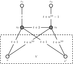
Figure 3: Illustration of the infinity gadget. Gray vertices need to be added to the feedback vertex set.

Lastly, consider two vertices $v,v^{\prime}\in V$. Note that before the addition of the infinity gadget, by construction of $G$ we have that $d(v,v^{\prime})\leq n^{9}+2$ or $d(v,v^{\prime})=\infty$. Furthermore, if $D$ is a Yes-instance, we have shown in the correctness proof of the reduction that the difference between the smallest label and the largest label is at most $n^{9}+1$. This implies that for a vertex pair $v,v^{\prime}\in V$ with $d(v,v^{\prime})=\infty$ we have in the periodic case with $\Delta=n^{11}$, that $d(v,v^{\prime})\geq n^{11}-n^{9}>n^{10}$. Which means, after adding the vertices and edges of the infinity gadget, we indeed have that $d(v,v^{\prime})=n^{10}$. For all vertex pairs $v,v^{\prime}$ where in the original construction we have $d(v,v^{\prime})\neq\infty$, we can also see that adding the infinity gadget and setting $\Delta=n^{11}$ does not change the duration of a fastest path from $v$ to $v^{\prime}$, since all newly added temporal paths have duration at least $n^{10}$. We can conclude that the originally constructed instance $D$ is a Yes-instance if and only if it remains a Yes-instance after adding the infinity gadget and setting $\Delta=n^{11}$.

3 Algorithms for Periodic TGR

In this section we provide several algorithms for Periodic TGR. By Theorem 2.1 we have that Periodic TGR is NP-hard in general, hence we start by identifying restricted cases where we can solve the problem in polynomial time.

We first show in Section 3.1 that in the case when the underlying graph $G$ of an instance $(D,\Delta)$ of Periodic TGR is a tree, then we can determine desired $\Delta$-periodic labeling $\lambda$ of $G$ in polynomial time. In Section 3.2 we generalize this result. We show that Periodic TGR is fixed-parameter tractable when parameterized by the feedback edge number of the underlying graph. Note that our parameterized hardness result (Theorem 2.3) implies that we presumably cannot replace the feedback edge number with the smaller parameter feedback vertex number, or any other parameter that is smaller than the feedback vertex number, such as e.g. the treewidth. Finally, in Section 3.3 we give a dedicated algorithm to solve Periodic TGR in polynomial time if the underlying graph is a cycle. Note that this is already implied by our FPT result, however the direct algorithm we provide is much simpler for this case.

We first start with defining certain notions, that will be of use when solving the problem.

Definition 3.1 (Travel delays).

Let $(G,\lambda)$ be a temporal graph satisfying conditions of Periodic TGR. Let $e_{1}=uv$ and $e_{2}=vz$ be two incident edges in $G$ with $e_{1}\cap e_{2}=v$. We define the travel delay from $u$ to $z$ at vertex $v$, denoted with $\tau_{v}^{uz}$, as the difference of the labels of $e_{2}$ and $e_{1}$, where we subtract the value of the label of $e_{1}$ from the label of $e_{2}$, modulo $\Delta$. More specifically:

$$\tau_{v}^{uz}\equiv\lambda(e_{2})-\lambda(e_{1})\pmod{\Delta}.$$ (1)

Similarly, $\tau_{v}^{zu}\equiv\lambda(e_{1})-\lambda(e_{2})\pmod{\Delta}$.

Intuitively, the value of $\tau_{v}^{uz}$ represents how long a temporal path waits at vertex $v$ when first taking edge $e_{1}=uv$ and then edge $e_{2}=vz$.

From the above definition and the definition of the duration of the temporal path $P$ we get the following two observations. Let $P=(v_{0},v_{1},\dots,v_{p})$ be the underlying path of the temporal path $(P,\lambda)$ from $v_{0}$ to $v_{p}$. Then $d(P,\lambda)=\sum_{i=1}^{p-1}\tau_{v_{i}}^{v_{i-1}v_{i}}+1$.

Proof 3.2.

For the simplicity of the proof denote $t_{i}=\lambda(v_{i-1}v_{i})$, and suppose that $t_{i}\leq t_{i+1}$, for all $i\in\{1,2,3,\dots,p\}$. Then

$$\sum_{i=1}^{p-1}\tau_{v_{i}}^{v_{i-1}v_{i}}+1 =\sum_{i=1}^{p-1}(t_{i+1}-t_{i})+1$$

$$=(t_{2}-t_{1})+(t_{3}-t_{2})+\cdots+(t_{p}-t_{p-1})+1$$

$$=t_{p-1}-t_{1}+1$$

$$=d(P,\lambda)$$

Now in the case when $t_{i}>t_{i+1}$ we get that $\tau_{v_{i}}^{v_{i-1}v_{i+1}}=\Delta+t_{i+1}-t_{i}$. At the end this still results in the correct duration as the last time we traverse the path $P$ is not exactly $t_{p}$ but $k\lambda+t_{p}$, for some $k$.

We also get the following. Let $(G,\lambda)$ be a temporal graph satisfying conditions of the Periodic TGRproblem. For any two incident edges $e_{1}=uv$ and $e_{2}=vz$ on vertices $u,v,z\in V$, with $e_{1}\cap e_{2}=v$, we have $\tau_{v}^{zu}=\Delta-\tau_{v}^{uz}\pmod{\Delta}$.

Proof 3.3.

Let $e_{1}=uv$ and $e_{2}=vz$ be two edges in $G$ for which $e_{1}\cap e_{2}=v$. By the definition $\tau_{v}^{uz}\equiv\lambda(e_{2})-\lambda(e_{1})\pmod{\Delta}$ and $\tau_{v}^{zu}\equiv\lambda(e_{1})-\lambda(e_{2})\pmod{\Delta}$. Summing now both equations we get $\tau_{v}^{uz}+\tau_{v}^{zu}\equiv\lambda(e_{2})-\lambda(e_{1})+\lambda(e_{1})-\lambda(e_{2})\pmod{\Delta}$, and therefore $\tau_{v}^{uz}+\tau_{v}^{zu}\equiv 0\pmod{\Delta}$, which is equivalent as saying $\tau_{v}^{uz}\equiv-\tau_{v}^{zu}\pmod{\Delta}$ or $\tau_{v}^{zu}=\Delta-\tau_{v}^{uz}\pmod{\Delta}$.

Lemma 3.4.

Let $(G,\lambda)$ be a temporal graph satisfying conditions of the Periodic TGRproblem, and let $(P,\lambda)=(P_{1,k},\lambda)$ be a fastest temporal path from $u=v_{1}$ to $v=v_{k}$ on $k$ vertices $v_{1},v_{2},\dots,v_{k}$. Let us denote with $(P_{1,i},\lambda)$ the sub-path of temporal path $(P_{1,k},\lambda)$, that starts at $v_{1}$ and finishes at $v_{i}$. Suppose that for any $v_{i}$ in $P$ it follows that $(P_{1,i},\lambda)$ is also the fastest temporal path from $u=v_{1}$ to $v_{i}$. Then we can determine travel delays on vertices of $P$ using the following equation

$$\tau_{v_{i}}^{v_{i-1},v_{i+1}}=D_{1,i+1}-D_{1,i},$$ (2)

for all $i\in\{2,3,\dots,k-1\}$.

Proof 3.5.

Let $(P,\lambda)$ be a fastest temporal path from $v_{1}$ to $v_{k}$ with the properties from the claim, and let $v_{i}$ be an arbitrary vertex in $P\setminus\{v_{1},v_{k}\}$. Using the properties of fastest paths and the definition of duration, we can rewrite Equation 2 as follows

$$\tau_{v_{i}}^{v_{i-1},v_{i+1}} =D_{1,i+1}-D_{1,i}=d(P_{1,i+1})-d(P_{1,i})$$

$$\equiv\left(\lambda(v_{i}v_{i+1})-\lambda(v_{1}v_{2})+1\right)-\left(\lambda(v_{i-1}v_{i})-\lambda(v_{1}v_{2})+1\right)\pmod{\Delta}$$

$$\equiv\lambda(v_{i}v_{i+1})-\lambda(v_{i-1}v_{i})\pmod{\Delta},$$

which is exactly the definition of $\tau_{v_{i}}^{v_{i-1},v_{i+1}}$.

3.1 Polynomial-time algorithm for trees

We are now ready to provide a polynomial-time algorithm for Periodic TGR when the underlying graph is a tree. Let $D$ be a matrix from Periodic TGR and let the underlying graph $G$ of $D$ be a tree on $n$ vertices $\{v_{1},v_{2},\dots,v_{n}\}$. Let $v_{i},v_{j}$ be two arbitrary vertices in $G$. Then we know that there exists a unique (static) path $P$ among them. Consequently, it follows that the temporal paths $(P_{i,j},\lambda)$ from $v_{i}$ to $v_{j}$ and $(P_{j,i},\lambda)$ from $v_{j}$ to $v_{i}$ are also unique, up to modulo of the period $\Delta$ of the labeling $\lambda$, and therefore are the fastest. Then $D$ is of the following fo:

$$D_{i,j}=\begin{cases}0&\text{if $i=j$},\\ 1&\text{if $v_{i}$ and $v_{j}$ are neighbours in G}\\ d(P_{i,j},\lambda)&\text{else}\end{cases},$$

where $d(P_{i,j},\lambda)$ is the duration of the (unique) temporal path $(P_{i,j},\lambda)$ from $v_{i}$ to $v_{j}$.

Let $v_{i},v_{j}$ be arbitrary two vertices in a tree $G$. Since there is a unique temporal path $(P_{i,j},\lambda)$ from $v_{i}$ to $v_{j}$, it is also the fastest one, therefore $d(P_{i,j},\lambda)=D_{i,j}$. Note, all other vertices $v^{\prime}\in P_{i,j}\setminus\{v_{i},v_{j}\}$ are reached form $v_{i}$ using a part of the path $(P_{i,j},\lambda)$. Now using Lemma 3.4, we can determine the waiting times for all inner vertices of the path $P_{i,j}$.

Theorem 3.6.

Periodic TGR can be solved in polynomial time on trees.

Proof 3.7.

Let $D$ be an input matrix for problem Periodic TGR of dimension $n\times n$. Let us fix the vertices of the corresponding graph $G$ of $D$ as $v_{1},v_{2},\dots,v_{n}$, where vertex $v_{i}$ corresponds to the row and column $i$ of matrix $D$. This can be done in polynomial time as we need to loop through the matrix $D$ once and connect vertices $v_{i},v_{j}$ for which $D_{i,j}=1$. At the same time we also check if $D_{i,i}=0$, for all $i\in[n]$. When $G$ is constructed we run DFS algorithm on it and check if it has no cycles. If at any step we encounter a problem, our algorithm stops and returns a negative answer.

From now on we can assume that we know that the underlying graph $G$ of $D$ is a tree and we know its structure. For the next part of the algorithm we use Section 3.1.

We pick an arbitrary vertex $v_{i}\in V(G)$ and check which vertex $v_{j}\in V(G)$ is furthest away from it, i. e., we find a maximum element in the $i$-th row of the matrix $D$. We now take the unique path $P_{i,j}$ in $G$, which has to also be the underlying path of the fastest temporal path from $v_{i}$ to $v_{j}$, and using Section 3.1 calculate waiting times at all inner vertices. We save those values in a matrix $T$, of size $n\times n\times n$, and mark vertices of the path $P_{i,j}$ as visited. Matrix $T$ stores at the position $(k,j,\ell)$ the value corresponding to the travel delay at vertex $v_{k}$ when traveling from $v_{j}$ to $v_{\ell}$, i. e., it stores the value $\tau_{v_{k}}^{v_{j},v_{\ell}}$, where $v_{j},v_{\ell}\in N(v_{k})$. All other values of $T$ are set to Null. Now we repeat procedure, from vertex $v_{i}$, for vertices that are not marked as visited yet, i. e., vertices in $V\setminus P_{i,j}$. We find a vertex in $V\setminus P_{i,j}$ that is furthest away from $v_{i}$ and repeat the procedure. When we have exhausted the $i$-th row of $D$, i. e., vertex $v_{i}$ now reaches every vertex of $G$, we continue and repeat the procedure for all other vertices. If at any point we get two different values for the same travel delay at a specific vertex, then we stop with the algorithm and return the negative answer. If the above procedure finishes successfully we get the matrix $T$ with travel delays for all vertices in $G$, of degree at least $2$. The above calculation is performed in polynomial time, as for every vertex $v_{i}$ we inspect the whole graph once.

Claim 18.

Matrix $T$ consists of travel delays for all vertices of degree at least $2$ in $G$.

Note, by the definition of travel delays, a vertex of degree $1$ cannot have a travel delay. Suppose now that there is a vertex $v_{i}\in V(G)$ of degree at least $2$, for which our algorithm did not calculate its travel delay. Let $v_{a},v_{b}$ be two arbitrary neighbors of $v_{i}$, i. e., $v_{a}v_{i},v_{i}v_{b}\in E(G)$. Since $G$ is a tree, the unique (and fastest) temporal path from $v_{a}$ to $v_{b}$ passes through $v_{i}$. When our algorithm was inspecting the row of $D$ corresponding to vertex $v_{a}$, it had to consider the temporal path from $v_{a}$ to $v_{b}$. At this point, it calculated $\tau_{v_{i}}^{v_{a},v_{b}}$. Since this is true for any two $v_{a},v_{b}\in N(v_{i})$, it cannot happen that some travel delay at $v_{i}$ is not calculated. Since $v_{i}$ was an arbitrary vertex in $G$ of degree at least $2$, the claim holds.

Now, given the matrix of travel delays $T$, we can find a labeling $\lambda$ that satisfies $D$. We start by fixing the label of an arbitrary edge as $a$, where $a\in[\Delta]$. Knowing the label of one edge, and all waiting times in $T$, we can uniquely determine the labels of all other edges. More specifically, if we know that $\lambda(v_{i}v_{j})=a$, then for all $v_{k}\in N(v_{i})$ (resp. $v_{k^{\prime}}\in N(v_{j})$) the value $\lambda(v_{i}v_{k})\equiv a+\tau_{v_{i}}^{v_{j},v_{k}}\pmod{\Delta}$ (resp. $\lambda(v_{j}v_{k^{\prime}})\equiv a+\tau_{v_{j}}^{v_{i},v_{k^{\prime}}}\pmod{\Delta}$). Since there are $\Delta$ options to fix the first label, we can find $\Delta$ different labelings satisfying $D$. Note, w.l.o.g. we can start determining the labeling $\lambda$ by setting $\lambda(v_{1}v_{2})=1$. It is not hard to see, that also the calculation of the labeling $\lambda$ takes polynomial time, as we have to traverse the graph exactly once, to successfully fix the labeling. Therefore, all together the whole algorithm is performed in polynomial time.

3.2 FPT-algorithm for feedback edge number

In this section we show how to generalize the result presented in Section 3.1. Following the distance-from-triviality parameterization paradigm [26, 38], we aim to obtain fixed-parameter tractability using a parameter that measures the distance from the underlying graph to a tree. Theorem 2.3 tells us that we presumably cannot use the feedback vertex number (or any smaller measure such as the treewidth) as a parameter to obtain tractability. Hence, we choose the feedback edge number as a parameter and we present an FPT algorithm for Periodic TGR parameterized by the feedback edge number of the underlying graph.

In a graph $G=(V,E)$, a feedback edge set $F\subset E(G)$ is a subset of edges, such that each cycle in $G$ has at least one edge in $F$. The minimum such set $F$ is called a minimum feedback edge set and its size, $k=|F|$, is called the feedback edge number of graph $G$. Note that one can find a minimum feedback edge set in linear time, by calculating a spanning tree (or forest) $T$ of the given graph $G$ and then removing all of the edges $T$ from $G$, i. e., $F=E(G)\setminus E(T)$.

Theorem 3.8.

Periodic Temporal Graph Realization is in FPT when parameterized by the feedback edge number of the underlying graph.

We first give an informal and very high-level description of the main ideas of the algorithm. It is well-known that the number of paths between two vertices in a static graph can be upper-bounded by a function of the feedback edge number of the graph. Intuitively, this would allow us to “guess” paths between a small number of vertex pairs in $G$ (the underlying graph of our instance Periodic TGR). These paths would then be used to create (representatives of) fastest temporal paths among vertex pairs in $(G,\lambda)$. We would then try to use the polynomial algorithm for trees (which includes paths) to figure out the labeling $\lambda$ of the edges used by these path. An idea like this has been used for several other temporal graph problems related to the connectivity between two vertices [14, 31, 21].

In our case, however, it is not enough to consider fastest temporal paths among some subset of vertices, but we have to determine the fastest temporal paths between all pairs of vertices. This means that we have to somehow extend the labeling $\lambda$ of the edges used by guessed paths to all other edges of $G$. Besides that we also need to make sure that all temporal paths that do not follow our guessed paths are not too fast.

A further difficulty arises from the somewhat unintuitive characteristic of fastest paths in temporal graphs. When considering the problem of finding shortest paths among vertices in static graphs, we have the nice property that if a shortest path $P$ from vertex $u$ to $v$ traverses the vertex $w$, then the subpath of $P$ from $u$ to $w$ is a shortest path from $u$ to $w$. This can help tremendously when developing algorithms. However, one can see that this property does not carry over to fastest paths in temporal graphs, for an example see Figure 4. For us this means that even if we guess a fastest path between two vertices, we cannot simply determine all labels of the edges used by the fastest path.

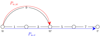
Figure 4: An example of a temporal graph, where the fastest temporal path $P_{u,v}$ (in blue) from $u$ to $v$ is of duration $7$, while the fastest temporal path $P_{u,w}$ (in red) from $u$ to a vertex $w$, that is on a path $P_{u,v}$, is of duration $1$ and is not a subpath of $P_{u,v}$.

To overcome the above mentioned difficulties, we propose the following high-level strategy.

• We identify a small number of “interesting vertices” between which we guess representative fastest paths.

• We show that we can determine most labels along each path up to an additive constant. We show that the number of labels we cannot determine along such a path is small.

• For each additive constant and each non-determined label along such a path we introduce a variable for an Integer Linear Program (ILP).

• We use constraints in the ILP to ensure that alternative connections (not using the guessed fastest path) between vertex pairs are not too fast.

• We compute a solution to the ILP and construct a labeling from that solution. Since the ILP has few variables and not too many constraints, this computation can be done efficiently using Lenstra’s Theorem [46].

For the remainder of this section, we fix the following notation. Let $D$ be the input matrix of Periodic TGR i. e., the matrix of the fastest temporal paths among $n$ vertices, and let $G$ be its underlying graph, on $n$ vertices and $m$ edges. With $F$ we denote a minimum feedback edge set of $G$, and with $k$ the feedback edge number of $G$. We are now ready to present our FPT algorithm. For an easier readability we split the description and analysis of the algorithm in five subsections. We start with a preprocessing procedure for graph $G$, where we define a set of interesting vertices which then allows us to guess the desired structures. Next we introduce some extra properties of our problem, that we then use to create ILP instances and their constraints. At the end we present how to solve all instances and produce the desired labeling $\lambda$ of $G$, if possible.

3.2.1 Preprocessing of the input

From the underlying graph $G$ of $D$ we first create a graph $G^{\prime}$ by iteratively removing vertices of degree one from $G$, and denote with

$$Z=V(G)\setminus V(G^{\prime}).$$

Then we determine a minimum feedback edge set $F$ of $G^{\prime}$. Note that $F$ is also a minimum feedback edge set of $G$. Lastly, we determine sets $U$, of vertices of interest, and $U^{*}$ of the neighbors of vertices of interest, in the following way. Let $T$ be a spanning tree of $G^{\prime}$, with $F$ being the corresponding feedback edge set of $G^{\prime}$. Let $V_{1}\subset V(G^{\prime})$ be the set of leaves in the spanning tree $T$, $V_{2}\subset V(G^{\prime})$ be the set of vertices of degree two in $T$, that are incident to at least one edge in $F$, and let $V_{3}\subset V(G^{\prime})$ be the set of vertices of degree at least $3$ in $T$. Then $|V_{1}|+|V_{2}|\leq 2k$, since every leaf in $T$ and every vertex in $V_{2}$ is incident to at least one edge in $F$, and $|V_{3}|\leq|V_{1}|$ by the properties of trees. We denote with

$$U=V_{1}\cup V_{2}\cup V_{3}$$

the set of vertices of interest. It follows that $|U|\leq 4k$. We set $U^{*}$ to be the set of vertices in $V(G^{\prime})\setminus U$ that are neighbors of vertices in $U$, i. e.,

$$U^{*}=\{v\in V(G^{\prime})\setminus U:u\in U,v\in N(u)\}.$$

Again, using the tree structure, we get that for any $u\in U$ its neighborhood is of size $|N(u)|\in O(k)$, therefore $|U^{*}|\in O(k^{2})$. From the construction of $Z$ (by iteratively removing vertices of degree one from $G$) it follows that $Z$ consists of disjoint trees $T_{1},T_{2},\dots$. For a tree $T_{i}$ we denote with $u_{i}$ the vertex in $G^{\prime}$ that is a neighbor of a vertex in $T_{i}$, and call it a clip vertex of the tree $T_{i}$. It follows that there can be many different trees $T_{i}$ that are incident to the same clip vertex $u_{i}\in V(G^{\prime})$, but each tree $T_{i}$ is incident to exactly one clip vertex $u_{i}\in V(G^{\prime})$. Since $u_{i}$ is the only vertex connecting all of the trees $T_{i}$ incident to it, from now on we assume that a tree $T_{u_{i}}$ in $Z$ is a union of trees on vertices from $V(G)\setminus V(G^{\prime})$, that are clipped at the same vertex $u_{i}\in V(G^{\prime})$. For each of the trees $T_{u_{i}}$ in $Z$, we select one vertex $r_{i}$, that is a neighbor of the clip vertex $u_{i}$, and call it a representative vertex of the tree $T_{u_{i}}$. We now define as $Z^{*}$ the set of representatives $r_{i}$ of trees $T_{i}\in Z$, where the clip vertex $v_{i}$ of $T_{i}$ is a vertex of interest, i. e.,

$$Z^{*}=\{r_{i}:r_{i}\in T_{i},\text{ where $T_{i}\in Z$, the clip vertex $u_{i}$ of $T_{i}$ is in $U$, and $r_{i}u_{i}\in E(G)$}\}.$$

Since there are $O(k)$ vertices of interest, we get that $|Z^{*}|\in O(k)$. Note that determining sets $U$, $U^{*}$, and $Z^{*}$ takes linear time.

Recall that a labeling $\lambda$ of $G$ satisfies $D$ if the duration of a fastest temporal path from vertex $v_{i}$ to $v_{j}$ equals $D_{v_{i},v_{j}}$. In order to find a labeling that satisfies this property we split our analysis in nine cases. We consider fastest temporal paths where the starting vertex is in one of the sets $U,V(G^{\prime})\setminus U,Z$, and similarly the destination vertex is in one of the sets $U,V(G^{\prime})\setminus U,Z$. In each of these cases we guess the underlying path $P$ that at least one fastest temporal path from the vertex $v_{i}$ to $v_{j}$ follows, which results in one equality constraint for the labels on the path $P$. For all other temporal paths from $v_{i}$ to $v_{j}$ we know that they cannot be faster, so we introduce inequality constraints for them. This results in producing $poly(n,m)$ constraints. Note that we have to do this while keeping the total number of variables upper-bounded by some function in $k$.

For an easier understanding and the analysis of the algorithm we give the following definition.

Definition 3.9.

Let $U\subseteq V(G^{\prime})$ be a set of vertices of interest and let $u,v\in U$. A path $P=(u=v_{1},v_{2},\dots,v_{p}=v)$ in graph $G^{\prime}$, where all inner vertices are not in $U$, i. e., $v_{i}\notin U$ for $i\in\{2,3,\dots,p-1\}$, is called a segment from $u$ to $v$. We denote it as $S_{u,v}$. Note $S_{u,v}\neq S_{v,u}$.

Observe that a temporal path in $G^{\prime}$ between two vertices of interest is either a segment, or consists of a sequence of some segments. Furthermore, since we have at most $4k$ interesting vertices in $G^{\prime}$, we can deduce the following important result.

Corollary 3.10.

There are at most $O(k^{2})$ segments in $G^{\prime}$.

3.2.2 Guessing necessary structures

Once the sets $U,U^{*}$ and $Z^{*}$ are determined, we are ready to start guessing the necessary structures. Note that whenever we say that we guess the fastest temporal path between two vertices, we mean that we guess the underlying path of a representative fastest temporal path between those two vertices. In the case when we want to guess the fastest path from $u$, that (somehow) passes through the vertex $x$, and goes directly to $v$ via an edge, we write it as a fastest path of form $u\leadsto x\rightarrow v$. Similarly it holds if we want to include more vertices that have to be visited by the path. If there is an edge (i. e., a unique fastest path) among two vertices, we denote it by $\rightarrow$, if the fastest path among two vertices is not uniquely determined, we denote it by $\leadsto$. We guess the following structures.

1. The fastest temporal paths among all pairs of vertices of $U$. For a pair $u,v$ of vertices in $U$, there are $k!$ possible paths in $G^{\prime}$ between them. Therefore, we have to try all $O(k^{k})$ possible paths, where at least one of them will be a fastest temporal path from $u$ to $v$, respecting the values from $D$. Repeating this procedure for all pairs of vertices $u,v\in U$ we get $O((k^{k})^{k^{2}})=O(k^{k^{3}})$ different variations of the fastest temporal paths among all vertices in $U$.

2. The fastest temporal paths among all vertices in $Z^{*}$, which by similar arguing as for vertices in $U$, gives us $O(k^{k^{3}})$ guesses.

3. The fastest temporal paths among all vertices in $U^{*}$. This gives us $O(k^{k^{6}})$ guesses.

4. The fastest temporal paths from vertices of $U$ to vertices in $U^{*}$, and vice versa, the fastest temporal paths from vertices in $U^{*}$ to vertices in $U$. This gives us $O(k^{k^{4}})$ guesses.

5. The fastest temporal paths from vertices of $U$ to vertices in $Z^{*}$, and vice versa. This gives us $O(k^{k^{3}})$ guesses.

6. The fastest temporal paths from vertices of $U^{*}$ to vertices in $Z^{*}$, and vice versa. This gives us $O(k^{k^{4}})$ guesses.

7. Let $S_{u,v}=(u=v_{1},v_{2},\dots,v_{p}=v)$ and $S_{w,z}=(w=z_{1},z_{2},\dots,z_{r}=z)$ be two segments, first one between vertices $u,v\in U$, second one between vertices $w,z\in U$. We want to guess the following fastest temporal path $v_{2}\rightarrow u\leadsto w\rightarrow z_{2}$. We repeat this procedure for all pairs of segments. Since there are $O(k^{2})$ segments in $G^{\prime}$, there are $O(k^{k^{5}})$ possible paths of this form.
   Recall that $S_{u,v}\neq S_{v,u}$ for every $u,v\in U$. Furthermore note that we did not assume that the sets $\{u,v\}$ and $\{w,z\}$ are disjoint. Therefore, by repeatedly making the above guesses, we also guess the following fastest temporal paths: ${v_{2}\rightarrow u\leadsto z\rightarrow z_{r-1}}$,   ${v_{2}\rightarrow u\leadsto v\rightarrow v_{p-1}}$,   ${v_{p-1}\rightarrow v\leadsto w\rightarrow z_{2}}$,   ${v_{p-1}\rightarrow v\leadsto z\rightarrow z_{r-1}}$, and ${v_{p-1}\rightarrow v\leadsto u\rightarrow v_{2}}$. For an example see Figure 5(a).

8. Let $S_{u,v}=(u=v_{1},v_{2},\dots,v_{p}=v)$ be a line segment in $G^{\prime}$, and let $w\in U\cup Z^{*}$ be either a vertex of interest or a representative vertex of a tree, whose clipped vertex is a of interest. We want to guess the following fastest temporal paths $w\leadsto u\rightarrow v_{2}$, $w\leadsto v\rightarrow v_{p-1}\rightarrow\cdots\rightarrow v_{2}$, and $v_{2}\rightarrow u\leadsto w$, $v_{2}\rightarrow v_{3}\rightarrow\cdots v\leadsto w$.
   For a fixed segment $S_{u,v}$ and a fixed vertex $w\in U\cup Z^{*}$ we have $O(k^{k})$ different possible such paths, therefore we make $O(k^{k^{4}})$ guesses for these paths. For an example see Figure 5(b).

9. Let $S_{u,v}=(u=v_{1},v_{2},\dots,v_{p}=v)$ be a line segment in $G^{\prime}$, and let us fix a vertex $v_{i}\in S_{u,v}\setminus\{u,v\}$. In the case when $S_{u,v}$ is of length $4$, the fixed vertex $v_{i}$ is the middle vertex (i. e., vertex that is on distance two from $u$ and $v$ in $S_{u,v}$). If $S_{u,v}$ is not of length $4$, we fix an arbitrary vertex $v_{i}\in S_{u,v}\setminus\{u,v\}$. Let $S_{w,z}=(w=z_{1},z_{2},\dots,z_{r}=z)$ be another segment in $G^{\prime}$. Note that all inner vertices of $S_{w,z}$ (i. e., vertices in $S_{w,z}\setminus\{w,z\}$) can be reached from $v_{i}$ by some path that has to go through $w$ or $z$. Therefore, the values of the duration of the fastest path from $v_{i}$ to vertices on the segment $S_{w,z}$ have to increase up to a certain point, when traversing the segment coming through $w$ and coming through $z$. We split the analysis into two cases.

   1. There is a single vertex $z_{j}\in S_{w,z}$ for which the duration from $v_{i}$ is the biggest. More specifically, $z_{j}\in S_{w,z}\setminus\{w,z\}$ is the vertex with the biggest value $D_{v_{i},z_{j}}$. We call this vertex a split vertex of $v_{i}$ in the segment $S_{wz}$. Then it holds that $D_{v_{i},z_{2}}<D_{v_{i},z_{3}}<\dots<D_{v_{i},z_{j}}$ and $D_{v_{i},z_{r-1}}<D_{v_{i},z_{r-2}}<\dots<D_{v_{i},z_{j}}$. From this it follows that the fastest temporal paths from $v_{i}$ to $z_{2},z_{3},\dots,z_{j-1}$ go through $w$, and the fastest temporal paths from $v_{i}$ to $z_{r-1},z_{r-2},\dots,z_{j+1}$ go through $z$. We now want to guess which vertex $w$ or $z$ is on a fastest temporal path from $v_{i}$ to $z_{j}$. Similarly, all fastest temporal paths starting at $v_{i}$ have to go either through $u$ or through $v$, which also gives us two extra guesses for the fastest temporal path from $v_{i}$ to $z_{j}$. Therefore, all together we have $4$ possibilities on how the fastest temporal path from $v_{i}$ to $z_{j}$ starts and ends. Besides that we want to guess also how the fastest temporal paths from $v_{i}$ to $z_{j-1},z_{j+1}$ start and end. Note that one of these is the subpath of the fastest temporal path from $v_{i}$ to $z_{j}$, and the ending part is uniquely determined for both of them, i. e., to reach $z_{j-1}$ the fastest temporal path travels through $w$, and to reach $z_{j+1}$ the fastest temporal path travels through $z$. Therefore we have to determine only how the path starts, namely if it travels through $u$ or $v$. This introduces two extra guesses. For a fixed $S_{u,v},v_{i}$ and $S_{w,z}$ we find the vertex $z_{j}$ in polynomial time, or determine that $z_{j}$ does not exist. We then make four guesses where we determine how the fastest temporal path from $v_{i}$ to $z_{j}$ passes through vertices $u,v$ and $w,z$ and for each of them two extra guesses to determine the fastest temporal path from $v_{i}$ to $z_{j-1}$ and from $v_{i}$ to $z_{j+1}$. We repeat this procedure for all pairs of segments, which results in producing $O(k^{k^{6}})$ new guesses. Note, $v_{i}\in S_{u,v}$ is fixed when calculating the split vertex for all other segments $S_{w,z}$.

   2. There are two vertices $z_{j},z_{j+1}\in S_{w,z}$ for which the duration from $v_{i}$ is the biggest. More specifically, $z_{j},z_{j+1}\in S_{w,z}\setminus\{w,z\}$ are the vertices with the biggest value $D_{v_{i},z_{j}}=D_{v_{i},z_{j+1}}$. Then it holds that $D_{v_{i},z_{2}}<D_{v_{i},z_{3}}<\dots<D_{v_{i},z_{j}}=D_{v_{i},z_{j+1}}>D_{v_{i},z_{j+2}}>\cdots>D_{v_{i},z_{r-1}}$. From this it follows that the fastest temporal paths from $v_{i}$ to $z_{2},z_{3},\dots,z_{j}$ go through $w$, and the fastest temporal paths from $v_{i}$ to $z_{r-1},z_{r-2},\dots,z_{j+1}$ go through $z$. In this case we only need to guess the following two fastest temporal paths $u\leadsto w\rightarrow z_{2}$ and $u\leadsto z\rightarrow z_{r-1}$. Each of this paths we then uniquely extend along the segment $S_{w,z}$ up to the vertex $v_{j}$, resp. $v_{j+1}$, which give us fastest temporal paths from $u$ to $v_{j}$ and from $u$ to $v_{j+1}$. Note that in this case we do not introduce any new guesses, as we have aready guessed the fastest paths of form $u\leadsto w\rightarrow z_{2}$ and $u\leadsto z\rightarrow z_{r-1}$ (see guess G-8).

   Note that this case results also in knowing the fastest paths from the vertex $v_{i}\in S_{u,v}$ to $w,z\in S_{w,z}$ for all segments $S_{w,z}$, i. e., we know the fastest paths from a fixed $v_{i}\in S_{u,v}$ to all vertices of interest in $U$. For an example see Figure 5(c).

10. Let $w\in U\cup Z^{*}$ be either a vertex of interest or a representative vertex of a tree, whose clipped vertex is a of interest, and let $S_{u,v}=(u=v_{1},v_{2},\dots,v_{p}=v)$ be a line segment in $G^{\prime}$. Similarly as above, in guess G-9, we want to guess a split vertex of $w$ in $S_{u,v}$, and the fastest temporal path that reaches it. We again have two cases, first one where $v_{i}$ is a unique vertex in $S_{u,v}$ that is furthest away from $w$, and the second one where $v_{i},v_{i+1}$ are two incident vertices in $S_{u,v}$, that are furthest away from $w$. In first case we know exactly how the fastest paths from $w$ to all vertices $v_{j}\in S_{u,v}\setminus\{v_{i}\}$ travel through the segment $S_{u,v}$ (i. e., either through $u$ or $v$). Therefore we have to guess how the fastest path from $w$ reaches vertex $v_{i}$, we have two options, either it travels through $u\rightarrow v_{2}\rightarrow\cdots\rightarrow v_{i-1}\rightarrow v_{i}$ or $v\rightarrow v_{p-1}\rightarrow\cdots\rightarrow v_{i+1}\rightarrow v_{i}$. Which produces two new guesses. In the second case we know exactly how the fastest temporal path reaches $v_{i}$ and $v_{i+1}$, and consequently all the inner vertices. Therefore no new guesses are needed. Note that the above guesses, together with the guesses from G-8, uniquely determine fastest temporal paths from $w$ to all vertices in $S_{u,v}$ (this also holds for the case when $w\in S_{u,v}$, i. e., $w=u$ or $w=v$).

    All together we make two guesses for each pair of vertex $w\in U$ and segment $S_{u,v}$. We repeat this for all vertices of interest, and all segments, which produces $O(k^{k^{2}})$ new guesses. For an example see Figure 5(d).

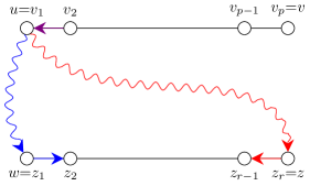
(a) Example of a guess G-7, where we guessed the fastest temporal paths of form $v_{2}\rightarrow u\leadsto w\rightarrow z_{2}$ (in blue) and $v_{2}\rightarrow u\leadsto z\rightarrow z_{r-1}$ (in red).

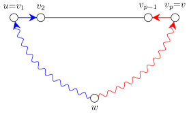
(b) Example of a guess G-8, where we guessed the fastest temporal paths of form $w\leadsto u\rightarrow v_{2}$ (in blue) and $w\leadsto v\rightarrow v_{p-1}$ (in red).

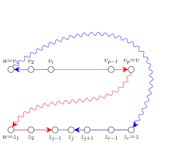
(c) Example of a guess G-9, where, for fixed a vertex $v_{i}\in S_{u,v}$, we calculated its corresponding split vertex $z_{j}\in S_{w,z}$, and guessed the fastest paths of form $v_{i}\rightarrow v_{i-1}\rightarrow\cdots\rightarrow u\leadsto z\rightarrow z_{r-1}\cdots\rightarrow z_{j}$ (in blue) and $v_{i}\rightarrow v_{i+1}\rightarrow\cdots\rightarrow v\leadsto w\rightarrow z_{2}\rightarrow\cdots\rightarrow z_{j-1}$ (in red).

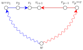
(d) Example of a guess G-10, where, for a vertex of interest $w$, we calculated its corresponding split vertex $v_{i}\in S_{u,v}$, and guessed the fastest paths of form $w\leadsto u\rightarrow v_{2}\rightarrow\cdots\rightarrow v_{i}$ (in blue) and $w\leadsto v\rightarrow v_{p-1}\rightarrow\cdots\rightarrow v_{i+1}$ (in red).

Figure 5: An example of guesses G-7, G-8, G-9 and G-10.

We create all of the guesses independently. We start with the first one, that results in $O(k^{k^{3}})$ different possibilities, then we split each one of these guesses into $O(k^{k^{3}})$ new ones, that respond to the guessing in the second step, etc. After creating all of the guesses we end up with $f(k)$ different cases (where $f$ is a double exponential). We now create one ILP instance for each case. From now on we assume that we know exactly the structure of all paths we have guessed.

3.2.3 Properties of Periodic TGR

In this section we study the properties of our problem, that then help us creating constraints of our ILP instances. Recall that with $G$ we denote our underlying graph of $D$. We want to determine labeling $\lambda$ of each edge of $G$. We start with an empty labeling of edges and try to specify each one of them. Note, that this does not necessarily mean that we assign numbers to the labels, but we might specify labels as variables or functions of other labels. We say that the label of an edge $f$ is determined with respect to the label of the edge edge $e$, if we have determined $\lambda(f)$ as a function of $\lambda(e)$.

In our analysis we exploit the following greatly, that is why we state is as an observation.

Let $P$ be the underlying path of a fastest temporal path from $u$ to $v$, where $e_{1},e_{p}\in P$ are its first and last edge, respectively. Then, knowing the label $\lambda(e_{1})$ of the first edge and the duration $d(P,\lambda)$ of the temporal path $(P,\lambda)$, we can uniquely determine the label $\lambda(e_{p})$ of the last edge of $P$. Symmetrically, knowing $\lambda(e_{p})$ and $d(P)$, we can uniquely determine $\lambda(e_{1})$. The correctness of the above statement follows directly from Definition 1.2. This is because the duration of $(P,\lambda)$ is calculated as the difference of labels of last and first edge plus $1$, where the label of last edge is considered with some delta periods, i. e., $d(P,\lambda)=p_{i}\Delta+\lambda(e_{p})-\lambda(e_{1})+1$, for some $p_{i}\geq 0$. Therefore $d(P,\lambda)\pmod{\Delta}\equiv(\lambda(e_{p})-\lambda(e_{1})+1)\pmod{\Delta}$. Note that if $\lambda(e_{1})$ and $\lambda(e_{p})$ are both unknown, then we can determine one with respect to the other.

In the following we prove that knowing the structure (the underlying path) of a fastest temporal path $P$ from a vertex of interest $u$ to a vertex of interest $v$, results in determining the labeling of each edge in the fastest temporal path from $u$ to $v$ (with the exception of some constant number of edges), with respect to the label of the first edge. More precisely, if path $P$ from $u$ to $v$ is a segment, then we can determine labels of all edges as a function of the label of the first edge. If $P$ consists of $\ell$ segments, then we can determine the labels of all but $\ell-1$ edges as a function of the label of the first edge. For the exact formulation and proofs see Lemmas 3.11 and 3.13.

Lemma 3.11.

Let $u,v\in U$ be two arbitrary vertices of interest and suppose that $P=(u=v_{1},v_{2},\dots,v_{p}=v)$, where $p\geq 2$, is a path in $G^{\prime}$, which is also the underlying path of a fastest temporal path from $u$ to $v$. Moreover suppose also that $P$ is a segment. We can determine the labeling $\lambda$ of every edge in $P$ with respect to the label $\lambda(uv_{2})$ of the first edge.

Proof 3.12.

We claim that $u$ reaches all of the vertices in $P$ the fastest, when traveling along $P$ (i. e., by using a subpath of $P$). To prove this suppose for the contradiction that there is a vertex $v_{i}\in P\setminus\{u,v\}$, that is reached from $v$ on a path different than $P_{i}=(u,v_{2},v_{3},\dots,v_{i})$ faster than through $P_{i}$. Since the only vertices of interest of $P$ are $u$ and $v$, it follows that all other vertices on $P$ are of degree $2$. Then the only way to reach $v_{i}$ from $u$, that differs from $P$, would be to go from $u$ to $v$ using a different path $P_{2}$, and then go from $v$ to $v_{p-1},v_{p-2},\dots,v_{i}$. But since $P$ is the fastest temporal path from $u$ to $v$, we get that $d(P_{2})\geq d(P)$ and $d(P_{2}\cup(v,v_{p-1},\dots,v_{i}))>d(P)>d(P_{i})$.

Now to label $P$ we use the fact that the fastest temporal path from $u$ to any $v_{i}\in P$ is a subpath of $P$, therefore we can label each edge using Section 3.2.3, where the duration from $u$ to $v_{i}$ equals to $D_{u,v_{i}}$ and we set the label of the first edge of $P$ to be a constant $c\in[\Delta]$. This gives us a unique label for each edge of $P$, that depends on the value $\lambda(uv_{2})$.

Lemma 3.13.

Let $u,v\in U$ be two arbitrary vertices of interest and suppose that $P=(u=v_{1},v_{2},\dots,v_{p}=v)$, where $p\geq 2$, is a path in $G^{\prime}$, which is also the underlying path of a fastest temporal path from $u$ to $v$. Let $\ell_{u,v}\geq 1$ be the number of vertices of interest in $P$ different to $u,v$, namely $\ell_{u,v}=|\{P\setminus\{u,v\}\}\cap U|$. We can determine the labeling $\lambda$ of all but $\ell_{u,v}$ edges of $P$, with respect to the label $\lambda(uv_{2})$ of the first edge, such that the labeling $\lambda$ respects the values from $D$.

For the proof of the above lemma, we first prove a weaker statement, for which we need to introduce some extra definitions and fix some notations. In the following we only consider wasteless temporal paths. We call a temporal path $P=((e_{1},t_{1}),\ldots,(e_{k},t_{k}))$ a wasteless temporal path, if for every $i=1,2,\ldots,k-1$, we have that $t_{i+1}$ is the first time after $t_{i}$ that the edge $e_{i+1}$ appears.

Let $u,v\in V$, and let $t\in\mathbb{N}$. Given that a temporal path starts within the period $[t,t+\Delta-1]$, we denote with $A_{t}(u,v)$ the arrival of the fastest path in $(G,\lambda)$ from $u$ to $v$, and with $A_{t}(u,v,P)$, the arrival along path $P$ in $(G,\lambda)$ from $u$ to $v$. Whenever $t=1$, we may omit the index $t$, i.e. we may write $A(u,v,P)=A_{1}(u,v,P)$ and $A(u,v)=A_{1}(u,v)$.

Suppose now that we know the underlying path $P_{u,v}=(u=v_{1},v_{2},\dots,v_{p}=v)$ of the fastest temporal path among vertices of interest $u$ and $v$ in $G^{\prime}$. Let $v_{i}\in U$ with $u\neq v_{i}\neq v$ be a vertex of interest on the path $P_{u,v}$. Suppose that $v_{i}$ is reached the fastest from $u$ by a path $P=(u=u_{1},u_{2},\dots,u_{j-1},v_{i})$. We split the path with $P_{u,v}$ into a path $Q=(u=v_{1},v_{2},\dots,v_{i})$ and $R=(v_{i},v_{i+1},\dots,v_{p}=v)$ (for details see Figure 6).

From the above we get the following assumptions:

1. $d(u,v_{i})=d(u,v_{i},P)\leq d(u,v_{i},Q)$, and

2. $d(u,v_{p})=d(u,v_{p},Q\cup R)\leq d(u,v_{p},P\cup R)$.

In the remainder, we denote with $\delta_{0}$ the difference $d(u,v_{i},Q)-d(u,v_{i})\geq 0$. Let $t_{v_{2}}\in[\Delta]$ be the label of the edge $uv_{2}$, and denote by $t_{u_{2}}$ the appearance of the edge $uu_{2}$ within the period $[t_{v_{2}},t_{v_{2}}+\Delta-1]$. Note that $1\leq t_{v_{2}}\leq\Delta$ and that $t_{v_{2}}\leq t_{u_{2}}\leq 2\Delta$. From Assumption 1 we get

$$\delta_{0}=d(u,v_{i},Q)-d(u,v_{i})=A_{t_{v_{2}}}(u,v_{i},Q)-A_{t_{v_{2}}}(u,v_{i},P)+\left(t_{u_{2}}-t_{v_{2}}\right)$$

and thus

$$A_{t_{v_{2}}}(u,v_{i},P)-A_{t_{v_{2}}}(u,v_{i},Q)=t_{u_{2}}-(t_{v_{2}}+\delta_{0}).$$ (3)

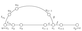
Figure 6: An example of the situation in Lemma 3.13, where we assume that the fastest temporal path from $u$ to $v$ is $P_{u,v}=(u=v_{1},v_{2},\dots v_{p})$, and the fastest temporal path from $u$ to $v_{i}$ in $P_{u,v}$ is $P=(u,u_{2},u_{3},\dots,v_{i})$. We denote with $Q=(u=v_{1},v_{2},\dots,v_{i})$ and with $R=(v_{i},v_{i+1},\dots,v_{p}=v)$.

We use all of the above discussion, to prove the following lemma.

Lemma 3.14.

If $t_{u_{2}}\neq t_{v_{2}}$, then $\delta_{0}\leq\Delta-2$ and $t_{u_{2}}\geq t_{v_{2}}+\delta_{0}+1$.

Proof 3.15.

First assume that $\delta_{0}\geq\Delta-1$. Then, it follows by Equation 3 that $A_{t_{v_{2}}}(u,v_{i},P)-A_{t_{v_{2}}}(u,v_{i},Q)\leq t_{u_{2}}-t_{v_{2}}-\Delta+1\leq 0$, and thus $A_{t_{v_{2}}}(u,v_{i},P)\leq A_{t_{v_{2}}}(u,v_{i},Q)$. Therefore, since we can traverse path $P$ from $u$ to $v_{i}$ by departing at time $t_{u_{2}}\geq t_{v_{2}}+1$ and by arriving no later than traversing path $Q$, we have that $d(u,v_{p},P\cup Q)<d(u,v_{p},Q\cup R)$, which is a contradiction to the second initial assumption. Therefore $\delta_{0}\leq\Delta-2$.

Now assume that $t_{v_{2}}+1\leq t_{u_{2}}\leq t_{v_{2}}+\delta_{0}$. Then, it follows by Equation 3 that $A_{t_{v_{2}}}(u,v_{i},P)\leq A_{t_{v_{2}}}(u,v_{i},Q)$ which is, similarly to the previous case, a contradiction. Therefore $t_{u_{2}}\geq t_{v_{2}}+\delta_{0}+1$.

The next corollary follows immediately from Lemma 3.14.

Corollary 3.16.

If $t_{u_{2}}\neq t_{v_{2}}$, then $1\leq A_{t_{v_{2}}}(u,v_{i},P)-A_{t_{v_{2}}}(u,v_{i},Q)\leq\Delta-1-\delta_{0}$.

We are now ready to prove the following result.

Lemma 3.17.

$d(u,v_{i-1},P\cup\{v_{i}v_{i-1}\})>d(u,v_{i-1},Q\setminus\{v_{i}v_{i-1}\})$.

Proof 3.18.

Let $e\in[\Delta]$ be the label of the edge $v_{i-1}v_{i}$, and let $f\in[e+1,e+\Delta]$ be the time of the first appearance of the edge $v_{i}v_{i+1}$ after time $e$. Let $A_{t_{v_{i}}}(u,v_{i},Q)=x\Delta+e$. Then $A_{t_{v_{i}}}(u,v_{i+1},Q\cup\{v_{i}v_{i+1}\})=x\Delta+f$. Furthermore let $g$ be such that $A_{t_{v_{i}}}(u,v_{i},P)=x\Delta+g$.

Case 1: $t_{u_{2}}\neq t_{v_{2}}$. Then Corollary 3.16 implies that $e+1\leq g\leq e+(\Delta-1-\delta_{0})$. Assume that $g<f$. Then, we can traverse path $P$ from $u$ to $v_{i}$ by departing at time $t_{u_{2}}\geq t_{v_{2}}+1$ and by arriving at most at time $x\Delta+f-1$, and thus $d(u,v_{p},P\cup R)<d(u,v_{p},Q\cup R)$, which is a contradiction to the second initial assumption. Therefore $g\geq f$. That is,

$$e+1\leq f\leq g\leq e+(\Delta-1-\delta_{0}).$$

Consider the path $P^{\ast}=P\cup\{v_{i}v_{i-1}\}$. Assume that we start traversing $P^{\ast}$ at time $t_{u_{2}}$. Then we arrive at $v_{i}$ at time $x\Delta+g$, and we continue by traversing edge $v_{i}v_{i-1}$ at time $(x+1)\Delta+e$. That is, $d(u,v_{i-1},P^{\ast})=(x+1)\Delta+e-t_{u_{2}}+1$.

Now consider the path $Q^{\ast}=Q\setminus\{v_{i}v_{i-1}\}$. Let $h\in[1,\Delta]$ be such that $A_{t_{v_{i}}}(u,v_{i-1},Q^{\ast})=x\Delta+e-h$. That is, if we start traversing $Q^{\ast}$ at time $t_{v_{2}}$, we arrive at $v_{i-1}$ at time $x\Delta+e-h$, i.e. $d(u,v_{i-1},Q^{\ast})=x\Delta+e-h-t_{v_{2}}+1$. Summarizing, we have:

$$d(u,v_{i-1},P^{\ast})-d(u,v_{i-1},Q^{\ast}) = \Delta+h-(t_{u_{2}}-t_{v_{2}})$$

$$\geq (\Delta-\delta_{0})+h>0,$$

which proves the statement of the lemma.

Case 2: $t_{u_{2}}=t_{v_{2}}$. Then, it follows by Equation (3) that $A_{t_{v_{2}}}(u,v_{i},P)=A_{t_{v_{2}}}(u,v_{i},Q)-\delta_{0}\leq A_{t_{v_{2}}}(u,v_{i},Q)$. Therefore $g\leq e$. Similarly to Case 1 above, consider the paths $P^{\ast}=P\cup\{v_{i}v_{i-1}\}$ and $Q^{\ast}=Q\setminus\{v_{i}v_{i-1}\}$. Assume that we start traversing $P^{\ast}$ at time $t_{u_{2}}=t_{v_{2}}$. Then we arrive at $v_{i}$ at time $x\Delta+g$, and we continue by traversing edge $v_{i}v_{i-1}$, either at time $(x+1)\Delta+e$ (in the case where $g=e$) or at time $x\Delta+e$ (in the case where $g\neq e$). That is, $d(u,v_{i-1},P^{\ast})\geq x\Delta+e-t_{v_{2}}+1$.

Similarly to Case 1, let $h\in[1,\Delta]$ be such that $A_{t_{v_{i}}}(u,v_{i-1},Q^{\ast})=x\Delta+e-h$. That is, if we start traversing $Q^{\ast}$ at time $t_{v_{2}}$, we arrive at $v_{i-1}$ at time $x\Delta+e-h$, i.e. $d(u,v_{i-1},Q^{\ast})=x\Delta+e-h-t_{v_{1}}+1$. Summarizing, we have:

$$d(u,v_{i-1},P^{\ast})-d(u,v_{i-1},Q^{\ast})\geq h\geq 1,$$

which proves the statement of the lemma.

From the above it follows that if $P$ is a fastest path from $u$ to $v$, then all vertices of $P$, with the exception of vertices of interest $v_{i}\in P\setminus\{u,v\}$, are reached using the same path $P$. We use this fact in the following proof.

Proof 3.19 (Proof of Lemma 3.13).

For every vertex of interest $v_{i}\in U\cap(P\setminus\{u,v\})$ we have two options. First, when the fastest temporal path $P^{\prime}$ from $u$ to $v_{i}$ is a subpath of $P$. In this case we determine the labeling of $P^{\prime}$ using Lemma 3.11. Second, when the fastest temporal path $P^{\prime}$ from $u$ to $v_{i}$ is not a subpath of $P$. In this case we know exactly how to label all of the edges of $P$, with the exception of edges of from $v_{i-1}v_{i}$, that are incident to $v_{i}$ in $P$.

Lemma 3.20.

Suppose that $S_{u,v},S_{w,z}$ are two segments with $v_{i}\in S_{u,v}$ and $z_{j}\in S_{w,z}$, where $z_{j}$ is a split vertex of $v_{i}$ in the segment $S_{w,z}$. W.l.o.g. suppose that the fastest temporal path from $v_{i}$ to $z_{j}$ travels through vertices $u$ and $w$. Then the fastest temporal path from $v_{i}$ to any other vertex of $S_{w,z}$, that is closer to $w$, travels through the same two vertices $u$ and $w$. Similarly it holds for the cases when the fastest temporal path travels through $w,v$ or $z,u$ or $z,v$.

Proof 3.21.

Let $z_{\ell}$ be a vertex of $S_{w,z}$, that is closer to $w$ than $z$ in the segment. Let us denote with $P_{v_{i},z_{j}}$ the underlying path of the fastest temporal path from $v_{i}$ to $z_{j}$. Denote with $P_{v_{i},z_{j}}^{\ell}$ the subpath of the fastest temporal path from $v_{i}$ to $z_{j}$, that terminates in $z_{\ell}$. We want to show that $P_{v_{i},z_{j}}^{\ell}$ is an underlying path of a fastest temporal path from $v_{i}$ to $z_{j}$. Let us observe the following possibilities.

First, suppose for the contradiction, that the fastest temporal path from $v_{i}$ to $z_{\ell}$ travels through vertices $u$ and $z$. Denote this path as $P^{1}_{v_{i},z_{\ell}}$. Then it follows that $d(P^{1}_{v_{i},z_{\ell}},\lambda)\leq d(P_{v_{i},z_{j}}^{\ell},\lambda)$, which would imply that the duration of the temporal path from $v_{i}$ to $z_{j}$ using the subpath of $P^{1}_{v_{i},z_{\ell}}$, would be strictly smaller than the duration of $(P_{v_{i},z_{j}},\lambda)$, which cannot be possible.

Second, suppose that the fastest temporal path from $v_{i}$ to $z_{\ell}$ travels through vertices $v$ and $w$. Denote this path as $P^{2}_{v_{i},z_{\ell}}$. Note that $P_{v_{i},z_{j}}^{\ell}$ and $P^{2}_{v_{i},z_{\ell}}$ intersect on a segment $S_{w,z}$ from the vertex $w$ to $z_{\ell}$. Therefore since $d(P^{2}_{v_{i},z_{\ell}},\lambda)\leq d(P_{v_{i},z_{j}}^{\ell},\lambda)$, and since there is unique way to extend the path $P^{2}_{v_{i},z_{\ell}}$ from $z_{\ell}$ to $z_{j}$, denote the extended path as $P^{j}_{v_{i},z_{\ell}}$, we get that $d(P^{j}_{v_{i},z_{\ell}},\lambda)\leq$$(P_{v_{i},z_{j}},\lambda)$. Which implies that $d(P^{j}_{v_{i},z_{\ell}},\lambda)=d(P_{v_{i},z_{j}},\lambda)$. Now using the similar argument it follows that $d(P_{v_{i},z_{j}}^{\ell},\lambda)=d(P^{2}_{v_{i},z_{\ell}},\lambda)$, therefore $P_{v_{i},z_{j}}^{\ell}$ is also a fastest temporal path from $v_{i}$ to $z_{j}$.

Third, suppose that the fastest temporal path from $v_{i}$ to $z_{\ell}$ travels through vertices $v$ and $z$. Denote this path as $P^{3}_{v_{i},z_{\ell}}$. Then the duration of the temporal path from $v_{i}$ to $z_{j}$ using the subpath of $P^{3}_{v_{i},z_{\ell}}$, would be strictly smaller than the duration of $(P_{v_{i},z_{j}},\lambda)$, which cannot be possible.

Lemma 3.22.

Let $S_{u,v}$ be a segment in $G$ of length at least $5$, i. e., $S_{u,v}=(u=v_{1},v_{2},\dots,v_{p}=v)$, where $p>5$. It cannot happen that an inner edge $f=v_{i}v_{i+1}$ from $S_{u,v}\setminus\{u,v\}$, is not a part of any fastest temporal path, of length at least $2$, among vertices in $S_{u,v}$, i. e., there has to be a pair $v_{j},v_{j^{\prime}}\in S_{u,v}$ s. t., the fastest temporal path from $v_{j}$ to $v_{j^{\prime}}$ passes through edge $f$. In the case when $p=5$ all temporal paths of length $2$ avoid $f$ if and only if $f$ has the same label as both of the edges incident to it.

Proof 3.23.

For an easier understanding and better readability we present the proof for $S_{u,v}$ of fixed length $5$. The case where $S_{u,v}$ is longer easily follows from presented results.

Let $S_{u,v}=(u=v_{1},v_{2},v_{3},v_{4},v_{5},v_{6}=v)$. We distinguish two cases, first that $f=v_{2}v_{3}$ (note that the case with $f=v_{4}v_{5}$ is symmetrical), and the second that $f=v_{3}v_{4}$. Throughout the proof we denote with $t_{i}$ the label of edge $v_{i}v_{i+1}$. Suppose for the contradiction, that none of the fastest temporal paths among vertices of $S_{u,v}$ traverses the edge $f$.

Case 1: $f=v_{2}v_{3}$. Let us observe the case of fastest temporal paths among $v_{1}$ and $v_{3}$. Denote with $Q=(v_{1},v_{2},v_{3})$ and with $P^{\prime}=(v_{3},v_{4},v_{5},v_{6})$. From our proposition it follows that

• the fastest temporal path $P^{+}$ from $v_{1}$ to $v_{3}$ is of the following form $P^{+}=v_{1}\leadsto v_{6}\rightarrow v_{5}\rightarrow v_{4}\rightarrow v_{3}$, and

• the fastest temporal path $P^{-}$ from $v_{3}$ to $v_{1}$ is of the following form $P^{-}=v_{3}\rightarrow v_{4}\rightarrow v_{5}\rightarrow v_{6}\leadsto v_{1}$.

It follows that $d(v_{1},v_{3},P^{+})\leq d(v_{1},v_{3},Q),$ and $d(v_{1},v_{3},P^{-})\leq d(v_{1},v_{3},Q)$. Let Note that $d(v_{1},v_{3},P^{+})\geq 1+d(v_{6},v_{3},P^{\prime})$, and by the definition $d(v_{6},v_{3},P^{\prime})=1+(t_{4}-t_{5})_{\Delta}+(t_{3}-t_{4})_{\Delta}$, where $(t_{i}-t_{j})_{\Delta}$ denotes the difference of two consecutive labels $t_{i},t_{j}$ modulo $\Delta$. Similarly holds for $d(v_{1},v_{3},P^{+})$. Summing now both of the above equations we get

$$\begin{split}d(v_{1},v_{3},P^{+})+d(v_{3},v_{1},P^{-})&\leq d(v_{1},v_{3},Q)+d(v_{3},v_{1},Q)\\ 1+d(v_{6},v_{3},P^{\prime})+1+d(v_{3},v_{6},P^{\prime})&\leq d(v_{1},v_{3},Q)+d(v_{3},v_{1},Q)\\ 2+1+(t_{4}-t_{5})_{\Delta}+(t_{3}-t_{4})_{\Delta}+1+(t_{4}-t_{3})_{\Delta}+(t_{5}-t_{4})_{\Delta}&\leq 1+(t_{2}-t_{1})_{\Delta}+1+(t_{1}-t_{2})_{\Delta}\\ (t_{4}-t_{5})_{\Delta}+(t_{5}-t_{4})_{\Delta}+(t_{4}-t_{3})_{\Delta}+(t_{3}-t_{4})_{\Delta}+2&\leq(t_{2}-t_{1})_{\Delta}+(t_{1}-t_{2})_{\Delta}.\end{split}$$ (4)

Note that if $t_{i}\neq t_{j}$ we get that the sum $(t_{i}-t_{j})_{\Delta}+(t_{j}-t_{i})_{\Delta}$ equals exactly $\Delta$, and if $t_{i}=t_{j}$ the sum equals $2\Delta$. This follows from the definition of travel delays at vertices (see Section 3). Therefore we get from Equation 4, that the right part is at most $2\Delta$, while the left part is at least $2\Delta+1$, for any relation of labels $t_{1},t_{2},\dots,t_{5}$, which is a contradiction.

Case 2: $f=v_{3}v_{4}$. Here we consider the fastest paths among vertices $v_{2}$ and $v_{4}$. By similar arguments as above we get

$$(t_{5}-t_{1})_{\Delta}+(t_{4}-t_{5})_{\Delta}+(t_{5}-t_{4})_{\Delta}+(t_{1}-t_{5})_{\Delta}+2\leq(t_{3}-t_{2})_{\Delta}+(t_{2}-t_{3})_{\Delta},$$

which is impossible.

In the case when $S_{u,v}$ is longer, we would get even bigger number on the left hand side of Equation 4, so we conclude that in all of the above cases, it cannot happen that all fastest paths of length $2$, among vertices in $S{{}_{u},v}$, avoid an edge $f$.

Let us observe now the case when $S_{u,v}=(u=v_{1},v_{2},v_{3},v_{4},v_{5}=v)$ is of length $4$. Let $f=v_{2}v_{3}$ (the case with $f=v_{3}v_{4}$ is symmetrical). Suppose that the fastest temporal paths among $v_{1}$ and $v_{3}$ do not use the edge $f$. We denote with $R^{+}$ the fastest path from $v_{1}$ to $v_{3}$, which is of form $u\leadsto v\rightarrow v_{4}\rightarrow v_{3}$, and similarly with $R^{-}$ the fastest path from $v_{3}$ to $v_{1}$, which is of form $v_{3}\rightarrow v_{4}\rightarrow v\leadsto u$. We denote with $R^{\prime}=(v_{3},v_{4},v_{5})$ and with $S=(v_{1},v_{2},v_{3})$. Again we get the following.

$$\begin{split}d(v_{1},v_{3},R^{+})+d(v_{3},v_{1},R^{-})&\leq d(v_{1},v_{3},S)+d(v_{3},v_{1},S)\\ 1+d(v_{5},v_{3},R^{\prime})+1+d(v_{3},v_{5},R^{\prime})&\leq d(v_{1},v_{3},S)+d(v_{3},v_{1},S)\\ (t_{3}-t_{4})_{\Delta}+(t_{4}-t_{3})_{\Delta}+2&\leq(t_{2}-t_{1})_{\Delta}+(t_{1}-t_{2})_{\Delta}.\end{split}$$

The only case when the equation has a valid solution is when $t_{1}=t_{2}$ and $t_{3}\neq t_{4}$, since in this case the left hands side evaluates to $\Delta+2$, while the right side evaluates to $2\Delta$.

Repeating the analysis for the fastest paths among $v_{2}$ and $v_{4}$, we get that the only valid solution is when $t_{2}=t_{3}$ and $t_{1}\neq t_{4}$. Altogether, we get that $f$ is not in a fastest path of length $2$ in $S_{u,v}$ if and only if the label of edge $f$ is the same as the labels on the edges incident to it, while the last remaining edge has a different label.

3.2.4 Adding constraints and variables to the ILP

We start by analyzing the case where we want to determine the labels on fastest temporal paths among vertices of interest. We proceed in the following way. Let $u,v\in U$ be two vertices of interest and let $P_{u,v}$ be the fastest temporal path from $u$ to $v$. If $P_{u,v}$ is a segment we determine all the labels of edges of $P_{u,v}$, with respect to the label of the first edge (see Lemma 3.11). In the case when $P_{u,v}$ is a sequence of $\ell$ segments, we determine all but $\ell-1$ labels of edges of $P_{u,v}$, with respect to the label of the first edge (see Lemma 3.13). We call these $\ell-1$ edges, partially determined edges. After repeating this step for all pairs of vertices in $U$, the edges of fastest temporal paths from $u$ to $v$, where $u,v\in U$, are determined with respect to the label of the first edge of each path, or are partially determined. If the fastest temporal path among two vertices $u,v\in U$ is just an edge $e$, then we treat it as being determined, since it gets assigned a label $\lambda(e)$ with respect to itself. All other edges in $G^{\prime}$ are called the not yet determined edges. Note that the not yet determined edges are exactly the ones that are not a part of any fastest temporal path.

Now we want to relate the not yet determined segments with the determined ones. Let $S_{u,v}$ and $S_{w,z}$ be two segments. At the beginning we have guessed the fastest path from $v_{i}$ to all vertices in $S_{w,z}$ (see guess G-9). We did this by determining which vertices $z_{j},z_{j+1}$ in $S_{w,z}$ are furthest away from $v_{i}$ (remember we can have the case when $z_{j}=z_{j+1}$), and then we guessed how the path from $v_{i}$ leaves the segment $S_{u,v}$ (i. e., either through the vertex $u$ or $v$), and then how it reaches $z_{j}$ (in the case when $z_{j}\neq z_{j+1}$ there is a unique way, when $z_{j}=z_{j+1}$ we determined which of the vertices $w$ or $z$ is on the fastest path). W.l.o.g. assume that we have guessed that the fastest path from $v_{i}$ to $z_{j}$ passes through $w$ and $z_{j-1}$. Then the fastest temporal path from $v_{i}$ to $z_{j+1}$ passes through $z$. And all fastest temporal paths from $v_{i}$ to any $z_{j^{\prime}}\in S_{w,z}$ use all of the edges in $S_{w,z}$ with the exception of the edge $z_{j}z_{j+1}$. Using this information and Section 3.2.3, we can determine the labels on all edges, with respect to the first or last label from the segment $S_{u,v}$, with the exception of the edge $z_{j}z_{j+1}$. Therefore, all edges of $S_{w,z}$ but $z_{j}z_{j+1}$ become determined. Since we repeat that procedure for all pairs of segments, we get that for a fixed segment $S_{w,z}$ we end up with a not yet determined edge $z_{j}z_{j+1}$ if and only if this is a not yet determined edge in relation to every other segment $S_{u,v}$ and its fixed vertex $v_{i}$. We repeat this procedure for all pairs of segments. Each specific calculation takes linear time, since there are $O(k^{2})$ segments, this calculation takes $O(k^{4})$ time. At this point the edges of every segment are fully determined, with the exception of at most three edges per segment (the first and last edge and potentially one extra somewhere in the segment). We will now relate also these edges. More precisely, let $S_{u,v}=(u=v_{1},v_{2},\dots,v_{p}=v)$ be a segment with three not yet determined edges, and let $e_{i}=v_{i}v_{i+1}$ denote an edge of $S_{u,v}$. From the above procedure (when we were determining labels of edges of segments with each other) we conclude that all of the edges $e_{i}$ of $S_{u,v}$ are in the following relation. There are some edges $e_{1},e_{2},\dots e_{i-1}$, whose label is determined with respect to the label $\lambda(e_{1})$, we have an edge $f=e_{i}=v_{i}v_{i+1}$ which is not yet determined, and then there follow the edges $e_{i+1},e_{i+2},\dots,e_{p-1}$, whose labels are determined with respect to the $\lambda(e_{p-1})$. We want to now determine all of the edges in such segment $S_{u,v}$ with respect to just one edge (either the first or the last one). For this we use the fact that at least one of the temporal paths among vertices in $S_{u,v}$ has to pass through $f$, when $S_{u,v}$ has at least $5$ edges (see Lemma 3.22). We proceed as follows.

1. For every segment $S_{u,v}=(u=v_{1},v_{2},\dots,v_{p}=v)$ with a not yet determined edge $v_{i}v_{i+1}=f\in S_{u,v}$, we guess which of the following fastest temporal paths pass through the edge $f$, one of the fastest paths between $v_{i-1}$ and $v_{i+1}$ (either from $v_{i-1}$ to $v_{i+1}$, or vice versa), and one of the fastest paths between $v_{i}$ and $v_{i+2}$. We create $4$ guesses for each such segments, therefore we create $O(k^{2})$ new guesses in total, as there are at most $O(k^{2})$ segments.

Once we know which two fastest temporal paths pass through $f$, we can determine the label of edge $f$ with respect to the first edge of the segment (when considering the fastest temporal path between $v_{i-1}$ and $v_{i+1}$), and with respect to the last edge of the segment (when considering the fastest temporal path between $v_{i}$ and $v_{i+2}$). Both these steps together determine all of the labels of $S_{u,v}$ with respect to just one label. Note, from Lemma 3.22 it follows that the above procedure holds only for segments with at least $5$ edges. In the case when segment has $4$ edges, it can happen that the fastest temporal paths from above, do not traverse $f$. But in this case we get that $3$ labels of edges in the segment have to be the same, while one is different, which results in a segment with two not yet determined edges. In the case when the segment $S_{u,v}$ has just three, two or one edge, this procedure does not improve anything, therefore these segments remain with three, two or one not yet determined edges, respectively. From now on we refer to segments of length less than $4$.

At this point $G$ is a graph, where each edge $e$ has a value for its label $\lambda(e)$ that depends on (i. e., is a function of) some other label $\lambda(f)$ of edge $f$, or it depends on no other label. We now describe how we create variables and start building our ILP instances. For every edge $e$ in $G^{\prime}$ that is incident to a vertex of interest we create a variable $x_{e}$ that can have values from $\{1,2,\dots,\Delta\}$. Besides that we create one variable for each edge that is still not yet determined on a segment. Since each vertex of interest is incident to at most $k$ edges, and each segment has at most one extra not yet determined edge, we create $O(k^{2})$ variables. At the end we create our final guess.

1. We guess the permutation of all $O(k^{2})$ variables, together with the relation of each variable to the labels of edges incident to these not yet determined edges. Namely, for an edge $e$ that is not yet determined, we set its value to $x_{e}$ and check labels of all of its neighbors, which are determined by some other label, and variables of the not yet determined neighbors, and guess if $x_{e}$ is smaller, equal or bigger than the labels of the edges of its neighbors. So, for any two variables $x_{e}$ and $x_{f}$, we know if $x_{e}<x_{f}$ or $x_{e}=x_{f}$, or $x_{e}>x_{f}$, and for any neighboring edge $g$ of $e$ we know if $x_{e}<\lambda(g)$ or $x_{e}=\lambda(g)$, or $x_{e}>\lambda(g)$. This results in $O(k^{2}!)=O(k^{2k^{2}})=O(k^{k^{3}})$ guesses and consequently each of the ILP instances we created up to now is further split into $O(k^{k^{3}})$ new ones.

We have now finished creating all ILP instances. From Section 3.2.2 we know the structure of all guessed paths, to which we have just added also the knowledge of permutation of all variables. We proceed with adding constraints to each of our ILP instances. First we add all constraints for the labels of edges that we have determined up to now. We then continue to iterate through all pairs of vertices and start adding equality (resp. inequality) constraints for the fastest (resp. not necessarily fastest) temporal paths among them.

We now describe how we add constraints to a path. Whenever we say that a duration of a path gives an equality or inequality constraint, we mean the following. Let $P=(u=v_{1},v_{2},\dots,v_{p}=v)$ be the underlying path of a fastest temporal path from $u$ to $v$, and let $Q=(u=z_{1},z_{2},\dots,z_{r}=v)$ be the underlying path of another temporal path from $u$ to $v$. Then we know that $d(P,\lambda)=D_{u,v}$ and $d(Q,\lambda)\geq D_{u,v}$. Using Section 3 we create an equality constraint for $P$ of the form

$$D_{u,v}=\sum_{i=2}^{p-1}(\lambda(v_{i}v_{i+1})-\lambda(v_{i-1}v_{i}))_{\Delta}+1,$$ (5)

and an inequality constraint for $Q$

$$D_{u,v}\leq\sum_{i=2}^{r-1}(\lambda(z_{i}z_{i+1})-\lambda(z_{i-1}z_{i}))_{\Delta}+1.$$ (6)

In both cases we implicitly assume that if the difference of $(\lambda(z_{i}z_{i+1})-\lambda(z_{i-1}z_{i}))$ is negative, for some $i$, we add the value $\Delta$ to it (i. e., we consider the difference modulo $\Delta$), therefore we have the sign $\Delta$ around the brackets. Note that we know if the difference of two consecutive labels is positive or negative. In the case when two consecutive labels are determined with respect to the same label $\lambda(e)$ the difference among them is easy to determine, if one or both consecutive labels are not yet determined then we have guessed in what kind of relation they are (see guess G- 12). Therefore we know when $\Delta$ has to be added, which implies that Equations 5 and 6 are calculated correctly for all paths.

We iterate through all pairs of vertices $x,y$ and make sure that the fastest temporal path from $x$ to $y$ produces the equality constrain Equation 5, and all other temporal paths from $x$ to $y$ produce the inequality constraint Equation 6. For each pair we argue how we determine these paths.

Fastest paths among $u,v$ where $u\in U$ and $v\in V$.

First we consider the case when $u,v$ are two vertices of interest. This was the case that we partially studied at the beginning of the algorithm, that helped us determine certain labels of the graph. We now iterate again through all fastest temporal paths from $u$ to $v$ and introduce an equality constraint for them. We then continue through all of the paths from $u$ to $v$, and for every one, that is not the underlying path of a fastest temporal path, we add the inequality constraint. There are $O(k^{k})$ possible paths from $u$ to $v$ in $G^{\prime}$, therefore in this step we introduce $O(k^{k^{3}})$ constraints.

Fastest paths among $u,x$ where $u\in U$ and $x\in V(G^{\prime})\setminus U$.

Next we continue with the case of the fastest path from $u$ to $x$, where $u\in U$ and $x\in V(G^{\prime})\setminus U$. From the guesses G-8 and G-10 it follows that we know the fastest temporal paths from $u$ to all vertices in a segment $S_{w,v}$. In this case we create the equality constraint for the fastest path and iterate through all other paths, for which we introduce the inequality constraints. There are $O(k^{k})$ possible paths of $u\leadsto w$ (resp. $u\leadsto v$), and a unique way how to extend those paths from $w$ (resp. $v$) to reach $x$ in $S_{w,v}$. Therefore we add $O(k^{k})$ inequality constraints.

Now we proceed with the case of determining the fastest path from $x$ to $u$, where $x\in V(G^{\prime})\setminus U$ and $u\in U$. Let $x$ a vertex in the segment $S_{w,z}=(w=z_{1},z_{2},\dots,z_{r}=z)$. If $S_{w,z}$ is of length $3$ or less, then we already know the fastest temporal path from every vertex in the segment to $u$ (since $S_{w,z}$ has at most $2$ inner vertices, we determined the fastest temporal paths from them to $u$ in guess G-4). Therefore assume that $S_{w,z}$ is of length at least $4$. This implies that there are at most two not yet determined edges in it. We can easily compute the vertices $z_{i},z_{i+1}\in S_{w,z}\setminus\{w,z\}$ for which the fastest temporal path from $z_{i}$ to $u$ has the biggest duration. Denote with $P^{+}$ the fastest temporal path of form $z_{2}\rightarrow z\leadsto u$, and with $P^{-}$ the fastest temporal path of form $z_{r-1}\rightarrow w\leadsto u$. Note that we know these paths from guess G-8. Then we know that all vertices $z_{j}$ in $S_{w,z}\setminus\{z_{i},z_{i+1}\}$ that are closer to $w$ than $z_{i},z_{i+1}$ reach $u$ on the following fastest temporal path $(z_{j}\rightarrow z_{j-1}\rightarrow\cdots\rightarrow z_{2})\cup P^{+}$ and all the vertices $z_{j}$ in $S_{w,z}\setminus\{z_{i},z_{i+1}\}$ that are closer to $z$ than $z_{i},z_{i+1}$ reach $u$ on the following fastest temporal path $(z_{j}\rightarrow z_{j+1}\rightarrow\cdots\rightarrow z_{r-1})\cup P^{-}$. Since the first part of fastest paths is unique, and we know the second part is the fastest, the above paths are the fastest temporal paths. We still have to determine the fastest temporal paths from $z_{i},z_{i+1}$ to $u$. We distinguish the following two options.

1. $z_{i}\neq z_{i+1}$. Then the fastest temporal path from $z_{i}$ to $u$ is $(z_{i}\rightarrow z_{i-1}\rightarrow\cdots\rightarrow z_{2})\cup P^{+}$, and the fastest temporal path from $z_{i+1}$ to $u$ is $(z_{i+1}\rightarrow z_{i+2}\rightarrow\cdots\rightarrow z_{r-1})\cup P^{-}$.

2. $z_{i}=z_{i+1}$, i. e., let $z_{i}$ be the unique vertex, that is furthest away from $u$ in $S_{w,z}$. In this case we have to determine if the fastest temporal path from $z_{i}$ to $u$, goes first through vertex $z_{i-1}$ (and then through $w$), or it goes first through $z_{i+1}$ (and then through $z$). Since we know the values $D_{z_{i-1},u},D_{z_{i+1},u}$, and since there are at most two not yet determined labels in $S_{w,z}$, we can uniquely determine one of the following waiting times: the waiting time $\tau_{v_{i-1}}^{v_{i},v_{i-2}}$ at vertex $v_{i-1}$ when traveling from $v_{i}$ to $v_{i-2}$, or the waiting time $\tau_{v_{i+1}}^{v_{i},v_{i+2}}$ at vertex $v_{i+1}$ when traveling from $v_{i}$ to $v_{i+2}$. Suppose we know the former (for the latter case, analysis follows similarly). Then we set $c=D_{z_{i-1},u}+\tau_{v_{i-1}}^{v_{i},v_{i-2}}$. We now compare $c$ and the value $D_{z_{i},u}$. If $c<D_{z_{i},u}$ we conclude that our ILP has no solution and we stop with calculations, if $c=D_{z_{i},u}$ then the fastest temporal path from $z_{i}$ to $u$ is of form $(z_{i}\rightarrow z_{i-1}\rightarrow\cdots\rightarrow z_{2})\cup P^{+}$, if $c>D_{z_{i},u}$ then the fastest temporal path from $z_{i}$ to $u$ is of form $(z_{i}\rightarrow z_{i+1}\rightarrow\cdots\rightarrow z_{r-1})\cup P^{-}$.

Once the fastest temporal paths are determined and we introduce the equality constraints for them. For all other $O(k^{k})$ paths (which correspond to all paths of form $w\leadsto u$ and $z\leadsto u$, together with the unique subpath on $S_{w,z}$), we introduce the inequality constraints.

Fastest paths among $x,y$ where $x\in V(G^{\prime})\setminus U$ and $y\in V(G^{\prime})\setminus U$.

Next is the case of determining the fastest path from $x$ to $y$, where $x,y\in V(G^{\prime})\setminus U$. We have two options.

1. Vertices $x,y$ are in the same segment $S_{u,v}=(u,v_{1},v_{2},\dots,v_{p},v)$. If the length of $S_{u,v}$ is less than $4$ then we know what is the fastest path among vertices. Suppose now that $S_{u,v}$ is of length at least $5$. Then there are at most two not yet determined edges in $S_{u,v}$.

   W.l.o.g. suppose that $x$ is closer to $u$ in $S_{u,v}$ than $y$. Denote with $x=v_{i}$. Let $v_{k}\in S_{u,v}$ be a vertex for which the duration from $v_{i}$ is the biggest (note that in the case when we have two such vertices, $v_{k}$ and $v_{k+1}$ we know exactly what are the fastest paths from $x$ to every vertex in $S_{u,v}$, by similar arguing as in case (i) from above, when we were determining the fastest path from $x\in V(G^{\prime})$ to $u\in U$. Then we know that $D_{x,v_{i+1}}<D_{x,v_{i+2}}<\cdots<D_{x,v_{k}}$ and $D_{x,v_{i-1}}<D_{x,v_{i-2}}<\cdots<D_{x,v_{k}}$, where indices are taken modulo $p$. Therefore we know exactly the structure of all the fastest paths from $x$ to every vertex in $S_{u,v}$, with the exception of the fastest path from $x$ to $v_{k}$. Since there is at most one undetermined edge in $S_{u,v}$, and since we know the exact durations $D_{x,v_{k-1}}$ and $D_{x,v_{k+1}}$, we can determine either $c=D_{x,v_{k-1}}+\tau_{v_{k}-1}^{v_{k},v_{k-2}}$ or $c^{\prime}=D_{x,v_{k+1}}+\tau_{v_{k}+1}^{v_{k},v_{k+2}}$. We then compare (one of) these values to $D_{x,v_{k}}$ which then uniquely determines the fastest temporal path from $x$ to $v_{k}$ (for details see case (ii) from above, when we were determining the fastest path from $x\in V(G^{\prime})$ to $u\in U$).

2. Vertices $x$ and $y$ are in different segments. Let $x$ be a vertex in the segment $S_{u,v}=(u=v_{1},v_{2},\dots,v_{p}=v)$ and let $y$ be a vertex in the segment $S_{w,z}=(w=z_{1},z_{2},z_{3},\dots,z_{r}=z)$. By checking the durations of the fastest paths from $x$ to every vertex in $S_{w,z}\setminus\{w,z\}$ we can determine the vertex $z_{i}\in S_{w,z}$, for which the duration from $x$ is the biggest. Note that if there are two such vertices $z_{i}$ and $z_{i+1}$, we know exactly how all fastest temporal paths enter $S_{w,z}$ (we use similar arguing as in case (i) from above, when we were determining the fastest path from $x\in V(G^{\prime})$ to $u\in U$). This implies that the fastest temporal paths from $x$ to all vertices $z_{2},z_{3},\dots,z_{i-1}$ (resp. $z_{i+1},z_{i+2},\dots,z_{r-1}$) pass through $w$ (resp. $z$). Now we determine the vertex $v_{j}\in S_{u,v}\setminus\{u,v\}$, for which the value of the durations of the fastest paths from it to the vertex $y$ is the biggest. Again, if there are two such vertices $v_{j}$ and $v_{j+1}$ we know exactly how the fastest temporal paths, starting in these two vertices, leave the segment $S_{u,v}$. We use similar arguing as in case (i) from above, when we were determining the fastest path from $x\in V(G^{\prime})$ to $u\in U$. Knowing the vertex $v_{j}$ implies that the fastest temporal paths from the vertices $v_{2},v_{2},\dots,v_{j-1}$ (resp. $v_{j+1},v_{j+2},\dots,v_{p-1}$) to the vertex $y$ passes through $u$ (resp. $v$). Since we know the following fastest temporal paths (see guess G-7) $z_{2}\rightarrow w\leadsto u\rightarrow v_{2}$, $z_{2}\rightarrow w\leadsto v\rightarrow v_{p-1}$, $z_{r-1}\rightarrow z\leadsto v\rightarrow v_{p-1}$ and $z_{r-1}\rightarrow z\leadsto v\rightarrow v_{p-1}$, we can uniquely determine all fastest temporal paths from $x\neq v_{j}$ to any $y\in S_{u,v}\setminus\{z_{i}\}$.

   We have to now consider the case when $x=v_{j}$ and $y=z_{i}$. If at least one of the segments $S_{u,v}$ and $S_{w,z}$ is of length more than $5$, then this segment has no inner edges with not yet determined labels and we can uniquely determine the fastest path from $v_{j}$ to $z_{i}$, using similar arguing as in case (ii) from above, when we were determining the fastest path from $x\in V(G^{\prime})$ to $u\in U$. If at least one of them is of length $3$ or less, we can again uniquely determine the fastest path from $v_{j}$ to $z_{i}$, using the same approach, and the knowledge of fastest paths to (or from) all vertices of the segment of length $3$ (as we guessed them in guess G-7). If both segments are of the length $4$, then we know how all vertices reach each other, as we guessed the fastest paths in guesses G-7 and G-9.

Once the fastest paths are uniquely determined we introduce the equality constraints for them and iterate through all other paths, that produce inequalities. To find all non-fastest temporal paths we have to consider all possible paths $u\leadsto w$ among vertices of interest, that are the endpoints of observed segments, once the segment is reached there is a unique path how to traverse it. Therefore we introduce $O(k^{k})$ inequality constraints for each pair of vertices $x,y$.

Considering the paths for vertices from $Z$.

All of the above is enough to determine the labeling $\lambda$ of $G^{\prime}$. Now we have to make sure that the labeling considers also the vertices in $Z$ that we initially removed from $G$. Remember that removed vertices form disjoint trees in $G$. Let us denote $Z$ as the set of disjoint trees, i. e., $Z=T_{1}\cup T_{2}\cup\cdots\cup T_{t}$, where $T_{i}$ represents one of the trees. Since there is a unique (static) path between any two vertices $z_{1},z_{2}$ in a tree $T_{i}$, it follows that there is also a unique (therefore also the fastest) temporal path among them. Thus determining the label of an edge in $T_{i}$ uniquely determines the labels on all other edges of tree $T_{i}$. Let us describe now how to determine the labels on edges of an arbitrary $T_{i}\in Z$. Recall that for every tree $T_{i}$ there is a representative vertex $v_{i}$ of $T_{i}$, and a clip vertex $u_{i}\in V(G^{\prime})$, such that $v_{i}\in N_{G}(u_{i})$. To determine the correct label of all edges of $T_{i}$ we use the following property.

Lemma 3.24.

Let $T_{i}$ be a tree in $Z$ and let $e_{i}=(u_{i},r_{i})$ be an edge in $G$, where $u_{i}\in V(G^{\prime})$ is a clip vertex of $T_{i}$ and $r_{i}\in T_{i}$ is a representative of $T_{i}$. Let $v\in N_{G^{\prime}}(u_{i})$ be the closest vertex to $r_{i}$, regarding the values of $D$, i. e., $D_{r_{i},v}\leq D_{r_{i},w}$ for all $w\in N_{G^{\prime}}(u)$. Then the path $P^{*}=(r_{i},u_{i},v)$ has to be the fastest temporal path from $r_{i}$ to $v$ in $G$.

Proof 3.25.

Suppose that this is not true. Then there exists a faster path $P^{*}_{2}$ from $r_{i}$ to $v$, that goes through the clip vertex $u_{i}$ of $T_{i}$ (as this is the only neighbor of $r_{i}$), through some other vertex $w\in N_{G^{\prime}}(u)\setminus\{v\}$, and through some other path $P^{\prime}$ in $G$, before it finishes in $v$, where $P^{\prime}$ is at least an edge (from $w$ to $v$). Therefore $P^{*}_{2}=(r_{i},u_{i},w,P^{\prime},v)$, where $d(P^{*}_{2})\leq d(P^{*})$. Now since $D_{r_{i},v}\leq D_{r_{i},w}$ for all $w\in N_{G^{\prime}}(u)$ the first part of path $P^{*}_{2}$ from $r_{i}$ to $w$ takes at least $D_{r_{i},v}$ time. Since $v\neq w$ we need at least one more time-step (one more edge) to traverse from $w$ to reach $v$. So $d(P^{*}_{2})\geq D_{r_{i},v}+1$, and so $P^{*}_{2}$ cannot be faster than $P^{*}$.

Suppose now that we know that $(r_{i},u_{i},v)$ is the fastest temporal path from the representative $r_{i}$ of $T_{i}$ to the vertex $v$ in the neighborhood of the clip vertex $v_{i}$ of $T_{i}$. Then we can determine the label of edge $r_{i}u_{i}$ as $\lambda(r_{i}u_{i})\equiv\lambda(u_{i}v)+1-D_{r_{i},v}\pmod{\Delta}$. Now, using the algorithm for trees (see Theorem 3.6), we determine labels on all edges of $T_{i}$. We repeat this procedure for all trees in $Z$. What remains, is to add the equality (resp. inequality) constraints for the fastest (resp. non-fastest) temporal paths from vertices of $Z$ to all other vertices in $G^{\prime}$ and vice versa. Note that since there is a unique path between vertices of tree $T_{i}$, and since all edges of tree $T_{i}$ are determined with respect to the same label, we present the study for cases when we find fastest temporal paths from and to the representative vertex $r_{i}$ of tree $T_{i}$. Each of these paths are then uniquely extended to all vertices in $T_{i}$.

Fastest paths among $z,u$ where $z\in Z$ and $u\in U$.

Let us start with the case when we want to determine the fastest temporal path from a representative vertex $r_{i}$ in some tree $T_{i}$ to a vertex of interest $u\in U$. We distinguish the following two cases.

1. The clip vertex $x$ of the tree $T_{i}$ is not a vertex of interest. Let $x=z_{i}$ be a part of a segment $S_{w,z}=(w=z_{1},z_{2},\dots,z_{r}=z)$, and denote with $z_{i-1}$ and $z_{i+1}$ the neighbouring vertices of $x$, where $z_{i-1}$ is closer to $w$ in $S_{w,z}$ and $z_{i+1}$ is closer to $z$ in $S_{w,z}$. From guess G-8 we know the following fastest paths $z_{2}\rightarrow w\leadsto u$ and $z_{r-1}\rightarrow z\leadsto u$. Denote thew with $Q_{1}$ and $Q_{r}$ respectively. There are two options.

   1. The segment $S_{w,z}$ is of length at least $5$ and has no not yet determined edges, with the exception of the first/last one. Which results in knowing all the waiting times at vertices of $S_{w,z}$ when traversing the segment. Then we also know that the labels of tree $T_{i}$ edges are determined with respect to that same edge label. This results in knowing the value of waiting time $\tau_{x}^{r_{i},z_{i-1}}$ at vertex $x$ when traversing it from $r_{i}$ to $z_{i-1}$ and the value of waiting time $\tau_{x}^{r_{i},z_{i+1}}$ at vertex $x$ when traversing it from $r_{i}$ to $z_{i+1}$. We also know the value $D_{x,u}$ and the underlying path of the fastest temporal path from $x$ to $u$ (which we determined in previous steps). W.l.o.g. suppose that the fastest path from $x$ to $u$ goes through $z_{i-1}$ and uses the path $Q_{1}$. Denote with $P^{-}=(r_{i},x,z_{i-1},z_{2})\cup Q_{1}$ and with $P^{+}=(r_{i},x,z_{i+1},z_{r-1})\cup Q_{r}$. Then we calculate the duration $d(P^{-})$ as $d(P^{-})=D_{x,u}+\tau_{x}^{r_{i},z_{i}-1}$ and compare it to $D_{r_{i},u}$. If $d(P^{-})<D_{r_{i},u}$ then we stop with the calculation and determine that our input graph has no solution. If $d(P^{-})=D_{r_{i},u}$ then we know that $P^{-}$ is the underlying path of the fastest temporal path from $r_{i}$ to $u$. If $d(P^{-})>D_{r_{i},u}$ then the fastest temporal path from $r_{i}$ to $u$ has to be $P^{+}$. For the fastest temporal path we introduce the equality constraint, for all other paths we introduce the inequality constraints. By similar arguing as in cases above, we introduce $O(k^{k})$ inequality constraints.

   2. The segment $S_{w,z}$ is of length $4$ or less and has an extra not yet determined edge $p$. If $p\cap\{x\}=\emptyset$, we can proceed with the same approach as above. So suppose now that $p=xz_{i+1}$. Then, from knowing that $p$ is a not yet determined edge we conclude that all fastest temporal paths from $x$ to any vertex of interest $u^{\prime}$ go through the edge $z_{i-1}x$, not trough $p$ (this is true as if a fastest temporal path from $x$ to some vertex of interest $w^{\prime}$ went through $p$, then $p$ would be determined). Now, if the edges of tree are determined with respect to the label of the edge $z_{i-1}x$ (not $p$), we use the same approach as above to determine the fastest temporal path from $r_{i}$ to $u$. Therefore, suppose that the edges of the tree $T_{i}$ are determined with respect to the label of the edge $p$. Which means that $D_{r_{i},z_{i+1}}<D_{r_{i},z_{i-1}}$. We want to now determine if the fastest temporal path from $r_{i}$ to $u$ is of form $r_{i}\rightarrow x\rightarrow z_{i-1}\rightarrow\dots\rightarrow w\leadsto u$ or $r_{i}\rightarrow x\rightarrow z_{i+1}\rightarrow\dots\rightarrow z\leadsto u$. We do the following. Denote with $c$ the value $c=D_{r_{i}z_{i-1}}+D_{xu}+1$. We now claim the following, note that we do not know what is the fastest temporal path from $r_{i}$ to $x_{i-1}$. It can be of the form $P^{-}=(r_{i},x,z_{i-1})$, or of the form $P^{+}=(r_{i},x,z_{i+1},z_{i+2},\dots,z)\cup Q\cup(w,z_{2},\dots,z_{i-1})$, where $Q$ is some path from $z$ to $w$. Denote with $R^{x}$ the underlying path of the fastest temporal path from $x$ to $u$, and with $R^{i-1}$ the underlying path of a fastest temporal path from $z_{i-1}$ to $u$. Note $R^{i-1}\subset R^{x}$. Similarly, denote with $R^{i+1}$ the underlying path of the fastest temporal path from $z_{i+1}$ to $u$, for which we know it goes through the vertex $z$.

      • If $c<D_{r_{i},u}$, then we have a contradiction and we stop with the calculation.
        This is true since we have found a temporal path from $r_{i}$ to $u$, with faster duration than the fastest temporal path from $r_{i}$ to $u$, which cannot happen.

      • If $c=D_{r_{i},u}$, then the fastest temporal path is of form $r_{i}\rightarrow x\rightarrow z_{i-1}\rightarrow\dots\rightarrow w\leadsto u$.
        We have two options, first when the fastest temporal path from $r_{i}$ to $z_{i-1}$ is $P^{-}$. In this case we have determined that $P^{-}\cup R^{i-1}$ is the fastest temporal path from $r_{i}$ to $u$. In the second case we suppose that the fastest temporal path from $r_{i}$ to $z_{i-1}$ is $P^{+}$. But then the duration of the path $P^{+}\cup R^{i-1}$ from $r_{i}$ to $u$ equals the duration of the fastest path from $r_{i}$ to $u$. But note that $P^{+}\cup R^{i-1}$ is actually not a path but a walk, since there is repetition of edges between $w$ and $z_{i-1}$, therefore it includes a path from $r_{i}$ to $u$, which is even faster, a contradiction. Therefore we get that in this case $P^{-}$ is always the underlying path of the fastest path from $r_{i}$ to $z_{i-1}$. And the fastest path from $r_{i}$ to $z_{i-1}$ is $P^{-}\cup R^{i-1}$.

      • If $c>D_{r_{i},u}$, then the fastest temporal path is of form $r_{i}\rightarrow x\rightarrow z_{i+1}\rightarrow\dots\rightarrow z\leadsto u$.
        We again have two options. First when the fastest temporal path from $r_{i}$ to $z_{i-1}$ is $P^{-}$. In this case we easily deduce that $P^{-}\cup R^{i-1}$ is not the underlying path of the fastest temporal path from $r_{i}$ to $u$. And therefore it follows that the the underlying path of the fastest temporal path from $r_{i}$ to $u$ is $(r_{i},x,z_{i+1})\cup R^{i+1}$. In the second case, suppose that $P^{+}$ is the underlying path of the fastest temporal path from $x_{i}$ to $z_{i-1}$. We want to now prove that the fastest temporal path from $r_{i}$ to $u$ travels through vertices $z_{i+1},z_{i+2},\dots z$. Suppose for the contradiction that this is not true. Then $S=(r_{i},x,z_{i-1})\cup R^{i-1}$ is the underlying path of the fastest temporal path from $r_{i}$ to $u$. Then we get that the duration $d(S)$ of $S$ equals to $D_{r_{i},u}$. Let $D(r_{i},z_{i-1},S)$ be the duration of the temporal path from $r_{i}$ to $z_{i-1}$ along the path $S$. By the definition we get that $d(S)=D(r_{i},z_{i-1},S)+D_{x,u}-1$. From this it follows that $D(r_{i},z_{i-1},S)=D_{r_{i},z_{i-1}}$, which is in contradiction with our assumption. Therefore we get that in this case $(r_{i},x,z_{i+1})\cup R^{i+1}$ is always the underlying path of the fastest path from $r_{i}$ to $z_{i-1}$.

      In all of the cases, we have uniquely determined the underlying path of the fastest temporal path from $r_{i}$ to $u$, which gives us an equality constraint. For all other paths we add the inequality constraints. There are $O(k^{k})$ of paths like this.

2. The clip vertex $w$ of the tree $T_{i}$ is a vertex of interest. In this case we know exactly the fastest path from a representative vertex $r_{i}$ to $u$ (we determined it in guess G-8). We create an equality constraint for this path, and create inequality constraints for all other paths. Since there are $O(k^{k})$ possible paths from $w$ to $u$, and there is a unique path (edge) from $r_{i}$ to $w$, we create $O(k^{k})$ inequality constraints. .

In the case when we want to determine the fastest path from a vertex of interest $u\in U$ to a representative vertex $r_{i}$ in $T_{i}$, we again have to split the analysis in two cases.

• The clip vertex $x\in S_{w,z}$ of $T_{i}$ is not a vertex of interest. In this case we know the fastest paths from $u$ to $x$, and to both of its neighbors $x_{i}$ and $x_{j}$, on the segment $S_{w,z}$, which is enough to determine the exact fastest path from $u$ to $r_{i}$ (we use the same procedure as in the case i when determining the fastest paths from $x$ to $u$).

• The clip vertex of $T_{i}$ is a vertex of interest. In this case we know exactly what is the fastest path (see guess G-8).

The procedure produces one equality constraint (for the fastest path) and $O(k^{k})$ inequality constraints.

Fastest paths among $z,y$ where $z\in Z$ and $y\in V(G^{\prime})\setminus U$.

The next two cases are the ones where we want to determine the fastest temporal path from a representative vertex $r_{i}$ in $T_{i}$, to some vertex $y\in V(G^{\prime})\setminus U$ that is not a vertex of interest, and vice versa. Since $y$ is not a vertex of interest it holds that $y\in S_{u,v}=(u=v_{1},v_{2},\dots,v_{p}=v)$. We use the similar approach as in the above case when we were determining paths between vertices in $Z$ and $U$, to determine the fastest temporal path from $r_{i}$ to $y$. The difference in this case is that we know the fastest temporal path from the clip vertex of $T_{i}$ to $y$ (when the clip vertex is not a vertex of interest), or we know the exact fastest path from the representative $r_{i}$ of $T_{i}$ to $y$ (when the clip vertex is a vertex of interest). The latter follows from the guess G-10.
Since $y\in S_{u,v}$ there are $O(k^{k})$ paths from the clip vertex to $y$, when the clip vertex is not a vertex of interest, and $O(k^{k})$ paths from the clip vertex to $y$, when the clip vertex is a vertex of interest. In all of the cases, we can uniquely determine the underlying path of the fastest temporal path from $r_{i}$ to $y$, which gives us an equality constraint. For all other paths we add the inequality constraints.

In the case when we want to determine the fastest path from a vertex $y\in V(G^{\prime})$, that is not a vertex of interest, to a representative vertex $r_{i}$ in $T_{i}$, we again have to split the analysis in two cases.

• The clip vertex $x\in S_{w,z}$ of $T_{i}$ is not a vertex of interest. In this case we know the fastest paths from $y$ to $x$, and to both of its neighbors $x_{i}$ and $x_{j}$, on the segment $S_{w,z}$, which is enough to determine the exact fastest path from $x$ to $r_{i}$ (we use the same procedure as in the case i when determining the fastest paths from $x$ to $u$).

• The clip vertex $u_{i}$ of $T_{i}$ is a vertex of interest. Let $y\in S_{u,v}=(u=v_{1},v_{2},\dots,v_{p}=v)$. In this case we know the fastest paths from $v_{2}$ and $v_{p-1}$ to $r_{i}$ (see guess G-8). Since the path from $y$ to $v_{2}$ (resp. $v_{p-1}$) is uniquely extended, we use the same procedure as in the case i, when determining the fastest paths from $x$ to $u$, to determine which is the fastest path from $y$ to $r_{i}$.

The procedure produces one equality constraint (for the fastest path) and $O(k^{k})$ inequality constraints.

Fastest paths among $z,z^{\prime}$ where $z\in Z$ and $z^{\prime}\in Z$.

The last case to consider is when we want to determine the fastest temporal paths among two vertices from $Z$. Let $r_{i},r_{j}$ be representative vertices of trees $T_{i}$ and $T_{j}$ and let $w_{i},w_{j}$ be their clip vertices, respectively. We distinguish following cases.

• Both clip vertices $w_{i},w_{j}$ are vertices of interest. In this case $r_{i},r_{j}\in Z^{*}$ and therefore we know the fastest paths among them (see guess G-8).

• One clip vertex is a vertex of interest and the other is not. Let $w_{i}\in U$ and $w_{j}\in S_{u,v}\setminus\{u,v\}$. Denote with $w_{j-1}$ and $w_{j+1}$ the two neighbors of $w_{j}\in S_{u,v}$. We know the fastest paths from the representative $r_{i}$ of tree $T_{i}$, to vertices $w_{j-1},w_{j},w_{j+1}$ (we determined them in the above case when we were determining the fastest paths from $z\in Z$ to $y\in V(G^{\prime})\setminus U$).

  Now we use the same procedure as in the case i, when determining the fastest paths from $x$ to $u$, to determine the exact fastest path from $r_{i}$ to $r_{j}$.

• None of the clip vertices $w_{i},w_{j}$ is a vertex of interest. Let $w_{i}\in S_{w,z}$ and $w_{j}\in S_{u,v}\setminus\{u,v\}$. Denote with $w_{j-1}$ and $w_{j+1}$ the two neighbors of $w_{j}\in S_{u,v}$, and similarly with $w_{i-1}$ and $w_{i+1}$ the two neighbors of $w_{i}\in S_{w,z}$. We know all the fastest paths from $r_{i}$ to $w_{j-1},w_{j},w_{j+1}$, and similarly all fastest paths from $r_{j}$ to $w_{i-1},w_{i},w_{i+1}$, together with all the fastest paths among each pair of the following vertices $w_{j-1},w_{j},w_{j+1}w_{i-1},w_{i},w_{i+1}$.

  Now we use the same procedure as in the case i, when determining the fastest paths from $x$ to $u$, to determine the exact fastest path from $r_{i}$ to $r_{j}$.

The procedure produces one equality constraint (for the fastest path) and $O(k^{k})$ inequality constraints.

3.2.5 Solving ILP instances

All of the above finishes our construction of ILP instances. We have created $f(k)$ instances (where $f$ is a double exponential function), each with $O(k^{2})$ variables and $n^{2}g(k)$ constraints (again, $g$ is a double exponential function). We now solve each ILP instance $I$, using results from Lenstra [46], in the FPT time, with respect to $k$. If none of the ILP instances gives a positive solution, then there exists no labeling $\lambda$ of $G$ that would realize the matrix $D$ (i. e., for any pair of vertices $u,v\in V(G)$ the duration of a fastest temporal path from $u$ to $v$ has to be $D_{u,v}$). If there is at least one $I$ that has a valid solution, we use this solution and produce our labeling $\lambda$, for which $(G,\lambda)$ realizes the matrix $D$. We have proven in the previous subsections that this is true since each ILP instance corresponds to a specific configuration of fastest temporal paths in the graph (i. e., considering all ILP instances is equivalent to exhaustively searching through all possible temporal paths among vertices). Besides that, in each ILP instance we add also the constraints for durations of all temporal paths among each pair of vertices. This results in setting the duration of a fastest path from a vertex $u\in V(G)$ to a vertex $v\in V(G)$ as $D_{u,v}$, and the duration of all other temporal paths from $u$ to $v$, to be greater or equal to $D_{u,v}$, for all pairs of vertices $u,v$. Therefore, if there is an instance with a positive solution, then this instance gives rise to the desired labeling, as it satisfies all of the constraints. For the other direction we can observe that if there is a labeling $\lambda$ meeting all duration requirements specified by $D$, then this labeling produces a specific configuration of fastest temporal paths. Since we consider all configurations, one of the produced ILP instances will correspond the configuration implicitly defined by $\lambda$, and hence our algorithm finds a solution.

To create the labeling $\lambda$ from a solution $X$, of a positive ILP instance, we use the following procedure. First we label each edge $e$, that corresponds to the variable $x_{e}$ by assigning the value $\lambda(e)=x_{e}$. We then continue to set the labels of all other edges. We know that the labels of all of the remaining edges depend on the label of (at least one) of the edges that were determined in previous step. Therefore, we easily calculate the desired labels for all remaining edges.

3.3 Polynomial-time algorithm for cycles

In this section, we present a polynomial-time algorithm for Periodic TGR when the underlying graph is a cycle. Note that Theorem 3.8 already implies that Periodic TGR on cycles is polynomial time solvable, however, for this particular case we can give a much simpler algorithm.

Let us observe some properties of the matrix $D$ from Periodic TGR, when the underlying graph $G$ of $D$ is a cycle $C_{n}=\{v_{1},v_{2},\dots,v_{n}\}$ on $n$ vertices. By the definition, each vertex is on distance $0$ from itself, and therefore also the duration $0$. This corresponds with all diagonal entries of $D$ being $0$. Now, let us observe that each vertex $v_{i}$ has exactly two neighbours in $C_{n}$, namely $v_{i-1}$ and $v_{i+1}$, therefore for all $i\in[n]$ we set $D_{i,i-1}=D_{i,i+1}=1$, where indices are taken modulo $n$. This results in the upper and lower diagonal of $D$ having all $1$’s, together with $D_{1,n}=D_{n,1}=1$. The matrix $D$ is of the following form

$$D=\begin{bmatrix}0&1&&&&1\\ 1&0&1&&&\\ &1&0&1&&\\ &&\ddots&\ddots&\ddots&\\ &&&1&0&1\\ 1&&&&1&0\end{bmatrix},$$ (7)

where the empty entries consists of positive integers different than $1$.

Given a matrix in the input of Periodic TGR we can check in $O(n^{2})$ time if it is of correct form, by traversing it once. If it is not of correct form, our algorithm stops and returns the negative answer. From now on, we assume, that the input matrix has the same form as $D$ from Equation 7.

Let $v_{i}$ be an arbitrary vertex in the cycle $C_{n}=\{v_{1},v_{2},\dots,v_{n}\}$. Vertex $v_{i}$ can reach an arbitrary vertex $v_{k}\in C_{n}$ using a positive side of the cycle (i. e., going from $v_{i}$ to $v_{i+1},v_{i+2}$, etc.), and using the negative side of the cycle (i. e., going from $v_{i}$ to $v_{i-1},v_{i-2}$, etc.). Let us denote with the $d^{+}(i,k)$ the duration of the temporal path from $v_{i}$ to $v_{k}$ using the positive side of the cycle, and with $d^{-}(i,k)$, the duration of the temporal path from $v_{i}$ to $v_{k}$ using the negative side of the cycle. Since these two are the only possible paths from $v_{i}$ to $v_{k}$ in $C_{n}$ we know that $D_{i,k}=min\{d^{+}(i,k),d^{-}(i,k)\}$.

Lemma 3.26.

If vertex $v_{i}$ reaches vertex $v_{j}$ the fastest, using the positive (resp. negative) side of the cycle, i. e., $v_{i},v_{i+1},\dots,v_{j-1},v_{j}$ (resp. $v_{i},v_{i-1},\dots,v_{j+1},v_{j}$), then $v_{i}$ reaches all other vertices $v_{k}$, where $k\in\{i+1,i+2,\dots,j-1\}$ (resp.  $k\in\{i-1,i-2,\dots,j+1\}$) using the same, positive (resp. negative) side of the cycle, where the indices are taken modulo $n$.

Proof 3.27.

Let $v_{i},v_{j}$ be two arbitrary vertices in $C_{n}$ and suppose that $D_{i,j}=d^{+}(i,j)$, but there exists a vertex $v_{k}$ from $C_{n}$, where $k\in\{i+1,i+2,\dots,j-1\}$, for which $D_{i,k}\neq d^{+}(i,k)$. Then $d^{-}(i,k)$ passes through vertex $v_{j}$, and we can split the path from $v_{i}$ to $v_{k}$ into two pieces, first from $v_{i}$ to $v_{j}$ and the second one from $v_{k}$ to $v_{j}$. So

$$d^{-}(i,k)=d^{-}(i,j)+d^{-}(j,k)^{*},$$ (8)

where $d^{-}(j,k)^{*}$ is the duration of the path from $v_{j}$ to $v_{k}$, using the negative side of the cycle, with consideration that we come to vertex $v_{j}$ at time $d^{-}(i,j)$ and we potentially have to wait there for some positive amount of time, before we continue to $v_{j}$ (i. e., $d^{-}(j,k)^{*}\geq d^{-}(i,j)\geq D_{j,k}$ includes some waiting time at vertex $v_{j}$). By the assumption we know that $d^{+}(i,j)\leq d^{-}(i,j)$, so we can rewrite Equation 8 as $d^{-}(i,k)\leq d^{+}(i,j)+d^{-}(j,k)^{*}$. This means that we can reach $v_{k}$ from $v_{j}$ by going from $v_{i}$ to $v_{j}$ using the positive side of the cycle, wait some time at $v_{j}$, before we continue back to $v_{j}$. In the above construction vertex $v_{k}$ is visited twice. By the definition, the fastest temporal path from $v_{i}$ to $v_{k}$ visits $v_{k}$ exactly once. Therefore we can stop at $v_{k}$ already when traveling from $v_{i}$ to $v_{j}$ the first time, using the positive side of the cycle. It follows that $D_{i,j}=d^{+}(i,j)\leq d^{-}(i,j)$, which contradicts with our assumption.

Let $v_{i}$ and $v_{j}$ be two arbitrary vertices in the cycle $C_{n}$, for which $v_{i}v_{j}\notin E(C_{n})$. Suppose that $P^{+}_{i,j}$ (resp. $P^{-}_{i,j})$ is the underlying path of the fastest temporal path from $v_{i}$ to $v_{j}$, using positive (resp. negative) side of the cycle, i. e., $v_{i},v_{i+1},\dots,v_{j-1},v_{j}$ (resp. $v_{i},v_{i-1},\dots,v_{j+1},v_{j}$). Then by Lemma 3.26 and Lemma 3.4, we get that we can determine all travel delays at vertices of $P^{+}_{i,j}\setminus\{v_{i},v_{j}\}$ (resp. $P^{-}_{i,j}\setminus\{v_{i},v_{j}\}$).

Let $v_{i}$ be an arbitrary vertex of $C_{n}$. Let us look at the row $i$ of the matrix $D$, which corresponds to the durations of fastest temporal paths from $v_{i}$ to all other vertices $v_{j}\in C_{n}$. Using Lemma 3.26 we know that $v_{i}$ will reach some consecutive vertices $v_{i+1},v_{i+2},\dots,v_{j}$ the fastest, using the positive side of the cycle and $v_{i-1},v_{i-2},\dots,v_{j+1}$ the fastest, using the negative side of the cycle. Suppose $v_{j}\in C_{n}$ is the last vertex $v_{i}$ reaches using the positive side of the cycle, and $v_{j+1}$ the last vertex that is reached using the negative side of the cycle. Then we know that $D_{i,i+1}<D_{i,i+2}<\cdots<D_{i,j-1}<D_{i,j}$ and $D_{i,i-1}<D_{i,i-2}<\cdots<D_{i,j+2}<D_{i,j+1}$. Note that it can happen that $v_{j}=v_{j+1}$, i. e., to reach vertex $v_{j}$ from $v_{i}$ the fastest, we can use either positive or negative side of the cycle. Using the above observations, every row $i$ ($i\in[n]$) of matrix $D$ has two (or one) maximum elements, one at position $j$ and the other at position $j+1$, where $j,j+1\in[n]$ and the indices are considered modulo $n$. Let us denote these two values as $m_{i}^{1}$ and $m_{i}^{2}$. The row $i$ of $D$ is of the following form, it has a $0$ at the entry $i$, it has $1$ at entries $i-1,i+1$, the values increase on the positions $i+1,i+2,i+3,\dots,j-1,j$ for some $j$ with value $m_{i}^{1}$, and on the other side, values increase on the positions $i-1,i-2,i-3,\dots,j+2,j+1$ for some $j+1$ with value $m_{i}^{2}$, where indices are taken modulo $n$.

Knowing this, we can split the vertices $v_{j}\in V(C_{n})\setminus\{v_{i}\}$ into two parts, ones that are reached from $v_{i}$ the fastest using the positive side of the cycle and ones that are reached using the negative side of the cycle. To determine these two sets we do the following. We fix a vertex $v_{i}\in C_{n}$ and check its corresponding row in the matrix $D$. We determine two max values $m_{i}^{1}$ and $m_{i}^{2}$ at positions $j$ and $j+1$ (modulo $n$), respectively, for which it has to hold that $D_{i,i+1}<D_{i,i+2}<\cdots<D_{i,j-1}<D_{i,j}=m_{i}^{1}$ and $D_{i,i-1}<D_{i,i-2}<\cdots<D_{i,j+2}<D_{i,j+1}=m_{i}^{2}$. Note, it can also happen that $m_{i}^{1}=m_{i}^{2}$. Now denote the path that uses the positive side of the cycle, from $v_{i}$ to $v_{j}$, as $P^{+}_{i}$ and the path that uses the negative side of the cycle, from $v_{i}$ to $v_{j+1}$, as $P^{-}_{i}$. By Lemma 3.26 and Lemma 3.4 we can calculate travel delays at every vertex $v_{k}\in C_{n}\setminus\{v_{i},v_{j},v_{j+1}\}$, which we store in a list $T$ of length $n$, where the entry at the position $k$ corresponds to the travel delay at vertex $v_{k}$ when traveling from $v_{k-1}$ to $v_{k+1}$. Note, from Section 3 it follows, that it is enough to store the value of the travel delay in one direction (i. e., knowing $\tau_{v}^{u,w}$ we know also $\tau_{v}^{w,u}$). We repeat the above procedure for all rows in the matrix $D$, i. e., for all vertices $v_{i}\in C_{n}$. Calculation in one row is performed in $O(n)$ time, repeating it for all rows we need $O(n^{2})$ time.

To determine the labeling $\lambda$ satisfying the matrix $D$, we have to make sure that we have calculated travel delays for all vertices.

Lemma 3.28.

List $T$ of travel delays has non-empty values at all positions, i. e., we have successfully calculated travel delays for all vertices.

Proof 3.29.

Throughout the proof we denote with $d^{+}(i,j)$ the duration of the temporal path that starts at $v_{i}$ and finishes at $v_{j}$, that uses the positive side of the cycle $C_{n}$, and similarly with $d^{-}(i,j)$ the duration of the temporal path that starts at $v_{i}$ and finishes at $v_{j}$, that uses the negative side of the cycle $C_{n}$, where indices are taken modulo $n$.

Suppose for the contradiction that the statement of the claim does not hold. Then there exists a vertex $v_{i}\in C_{n}$, for which we did not calculate its travel delay. Let $v_{j}\in C_{n}\setminus\{v_{i}\}$ be an arbitrary vertex. Note that the only time we cannot calculate the travel delay at vertex $v_{i}$, when considering vertex $v_{j}$, is in this case when $v_{i}$ is one of the maximum elements in $D_{j}$, i. e., $v_{i}$ is a vertex that is on a maximum duration from $v_{j}$. This has to hold for all vertices $v_{j}$, therefore $v_{i}$ has to be on the maximum duration from every vertex $v_{j}\in C_{n}\setminus\{v_{i}\}$. It then also has to hold for vertices $v_{i-1},v_{i+1}$, that are neighbours of $v_{i}$. We know that in this case $d^{+}(i-1,i)=1,d^{-}(i+1,i)=1$. Since $v_{i}$ has to be on the maximum duration from both of them (i. e., is one of the two maximum values $m^{1}_{i-1},m^{2}_{i-1}$ for vertex $v_{i-1}$ and one of the two maximum values $m^{1}_{i+1},m^{2}_{i+1}$ for vertex $v_{i+1}$), we know that

$$d^{+}(i+1,i-1)<d^{-}(i+1,i-1)$$ and (9)

$$d^{-}(i-1,i+1)<d^{+}(i-1,i+1).$$ (10)

If this would not hold, the fastest path would go through $v_{i}$ and we would be able to calculate the travel delay at $v_{i}$.

Denote the labels $\lambda(v_{i-1}v_{i})=a,\lambda(v_{i}v_{i+1})=a^{\prime}$, and $\lambda(v_{i-2}v_{i-1})=b,\lambda(v_{i+1}v_{i+2})=b^{\prime}$, where $a,a^{\prime},b,b^{\prime}\in[\Delta]$. W.l.o.g. we can suppose that $a\geq a^{\prime}$. Therefore, using the definition for the duration of temporal paths, we get that $d^{+}(i+1,i-1)=(k\Delta+b)-b^{\prime}+1$, where $k$ is some non-negative integer, and $d^{-}(i+1,i-1)=a-a^{\prime}+1$. Using the first inequality from Equation 9 we get that $(k\Delta+b)-b^{\prime}+1<a-a^{\prime}+1$ which is equivalent to $(k\Delta+b)-b^{\prime}<a-a^{\prime}$, which can be true only when $k=0$, but because the duration is positive we get that $b>b^{\prime}$ and $b-b^{\prime}<a-a^{\prime}$. Now again using the definition of the duration, we get $d^{+}(i-1,i+1)=(k\Delta+a^{\prime})-a+1$, where $k$ is some non-negative integer, but since $v_{i-1}v_{i}$ and $v_{i}v_{i+1}$ are incident edges, we know also that $k=1$, therefore $d^{+}(i-1,i+1)=\Delta+a-a+1$. Again by the definition, $d^{-}(i-1,i+1)=(k^{\prime}\Delta+b^{\prime})-b+1$, for some non-negative integer $k^{\prime}$. Using the second inequality from Equation 9 we get that $(k^{\prime}\Delta+b^{\prime})-b+1<\Delta+a-a+1$. Which is equivalent to $(k^{\prime}\Delta+b^{\prime})-b<\Delta+a^{\prime}-a$. This can hold only when $k^{\prime}=1$, in that case we get $\Delta+b^{\prime}-b<\Delta+a^{\prime}-a$ which is equivalent to $b^{\prime}-b<a^{\prime}-a$. This is in the contradiction with the inequality $b-b^{\prime}<a-a^{\prime}$ as this is equivalent to $b^{\prime}-b>a^{\prime}-a$.

Therefore it cannot happen that there is a vertex $v_{i}$ for which we cannot calculate its travel delay in $C_{n}$.

All of the above observations imply the following result.

Theorem 3.30.

Periodic TGR can be solved in polynomial time on cycles.

Proof 3.31.

As stated above, we can determine travel delays at every vertex in $O(n^{2})$ time. Once all of the delays are calculated, we have to only construct the labeling $\lambda$ that satisfies the matrix $D$. We start by fixing a label of one edge as $a$, where $a\in[\Delta]$. Knowing the label of edge $v_{1}v_{2}$ and all waiting times in $T$, we can uniquely determine the labels of all other edges. More specifically, if we know that $\lambda(v_{i}v_{j})=a$, then for all $v_{k}\in N(v_{i})$ (resp. $v_{k^{\prime}}\in N(v_{j})$) the value $\lambda(v_{i}v_{k})\equiv a+\tau_{v_{i}}^{v_{j},v_{k}}\pmod{\Delta}$ (resp. $\lambda(v_{j}v_{k^{\prime}})\equiv a+\tau_{v_{j}}^{v_{i},v_{k^{\prime}}}\pmod{\Delta}$). Since there are $\Delta$ options to fix the first label, we can find $\Delta$ different labelings satisfying $D$. Note, w.l.o.g. we can start determining the labeling $\lambda$ by setting $\lambda(v_{1}v_{2})=1$.

4 Conclusion

We have introduced a natural and canonical temporal version of the graph realization problem with respect to distance requirements, called Periodic Temporal Graph Realization. We have shown that the problem is NP-hard in general and polynomial-time solvable if the underlying graph is a tree. Building upon those results, we have investigated its parameterized computational complexity with respect to structural parameters of the underlying graph that measure “tree-likeness”. For those parameters, we essentially gave a tight classification between parameters that allow for tractability (in the FPT sense) and parameters that presumably do not. We showed that our problem is W[1]-hard when parameterized by the feedback vertex number of the underlying graph, and that it is in FPT when parameterized by the feedback edge number of the underlying graph. Note that most other common parameters that measure tree-likeness (such as the treewidth) are smaller than the vertex cover number.

We believe that our work spawns several interesting future research directions and builds a base upon which further temporal graph realization problems can be investigated.

Further parameterizations.

There are several structural parameters which can be considered to obtain tractability which are either larger or incomparable to the feedback vertex number.

• The vertex cover number measures the distance to an independent set, on which we trivially only have no-instances of our problem. We believe this is a promising parameter to obtain tractability.

• The tree-depth measures “star-likeness” of a graph and is incomparable to both the feedback vertex number and the feedback edge number. We leave the parameterized complexity of our problem with respect to this parameter open.

• Parameters that measure “path-likeness” such as the pathwidth or the vertex deletion distance to disjoint paths are also natural candidates to investigate.

Furthermore, we can consider combining a structural parameter with $\Delta$. Our NP-hardness reduction (Theorem 2.1) produces instances with constant $\Delta$, so as a single parameter $\Delta$ cannot yield fixed-parameter tractability. However, in our parameterized hardness reduction (Theorem 2.3) the value for $\Delta$ in the produced instance is large. This implies that our result does not rule out e.g. fixed-parameter tractability for the combination of the treewidth and $\Delta$ as a parameter. We believe that investigating such parameter combinations is a promising future research direction.

Further problem variants.

There are many natural variants of our problem that are well-motivated and warrant consideration. In the following, we give two specific examples. We believe that one of the most natural generalizations of our problem is to allow more than one label per edge in every $\Delta$-period. A well-motivated variant (especially from the network design perspective) of our problem would be to consider the entries of the duration matrix $D$ as upper-bounds on the duration of fastest paths rather than exact durations. Our work gives a starting point for many interesting future research directions such as the two mentioned examples.

References

- [1] Eleni C Akrida, Leszek Gąsieniec, George B. Mertzios, and Paul G Spirakis. The complexity of optimal design of temporally connected graphs. Theory of Computing Systems, 61:907–944, 2017.
- [2] Eleni C. Akrida, George B. Mertzios, Paul G. Spirakis, and Christoforos Raptopoulos. The temporal explorer who returns to the base. Journal of Computer and System Sciences, 120:179–193, 2021.
- [3] Emmanuel Arrighi, Niels Grüttemeier, Nils Morawietz, Frank Sommer, and Petra Wolf. Multi-parameter analysis of finding minors and subgraphs in edge-periodic temporal graphs. In Proceedings of the 48th International Conference on Current Trends in Theory and Practice of Computer Science (SOFSEM), pages 283–297, 2023.
- [4] John Augustine, Keerti Choudhary, Avi Cohen, David Peleg, Sumathi Sivasubramaniam, and Suman Sourav. Distributed graph realizations. IEEE Transactions on Parallel and Distributed Systems, 33(6):1321–1337, 2022.
- [5] Amotz Bar-Noy, Keerti Choudhary, David Peleg, and Dror Rawitz. Efficiently realizing interval sequences. SIAM Journal on Discrete Mathematics, 34(4):2318–2337, 2020.
- [6] Amotz Bar-Noy, Keerti Choudhary, David Peleg, and Dror Rawitz. Graph realizations: Maximum degree in vertex neighborhoods. In Proceedings of the 17th Scandinavian Symposium and Workshops on Algorithm Theory (SWAT), pages 10:1–10:17, 2020.
- [7] Amotz Bar-Noy, David Peleg, Mor Perry, and Dror Rawitz. Composed degree-distance realizations of graphs. In Proceedings of the 32nd International Workshop on Combinatorial Algorithms (IWOCA), pages 63–77, 2021.
- [8] Amotz Bar-Noy, David Peleg, Mor Perry, and Dror Rawitz. Graph realization of distance sets. In Proceedings of the 47th International Symposium on Mathematical Foundations of Computer Science (MFCS), pages 13:1–13:14, 2022.
- [9] Mehdi Behzad and James E Simpson. Eccentric sequences and eccentric sets in graphs. Discrete Mathematics, 16(3):187–193, 1976.
- [10] Robert E Bixby and Donald K Wagner. An almost linear-time algorithm for graph realization. Mathematics of Operations Research, 13(1):99–123, 1988.
- [11] Binh-Minh Bui-Xuan, Afonso Ferreira, and Aubin Jarry. Computing shortest, fastest, and foremost journeys in dynamic networks. International Journal of Foundations of Computer Science, 14(02):267–285, 2003.
- [12] Arnaud Casteigts, Timothée Corsini, and Writika Sarkar. Invited paper: Simple, strict, proper, happy: A study of reachability in temporal graphs. In Proceedings of the 24th International Symposium on Stabilization, Safety, and Security of Distributed Systems (SSS), pages 3–18, 2022.
- [13] Arnaud Casteigts, Paola Flocchini, Walter Quattrociocchi, and Nicola Santoro. Time-varying graphs and dynamic networks. International Journal of Parallel, Emergent and Distributed Systems, 27(5):387–408, 2012.
- [14] Arnaud Casteigts, Anne-Sophie Himmel, Hendrik Molter, and Philipp Zschoche. Finding temporal paths under waiting time constraints. Algorithmica, 83(9):2754–2802, 2021.
- [15] Wai-Kai Chen. On the realization of a -digraph with prescribed degrees. Journal of the Franklin Institute, 281(5):406–422, 1966.
- [16] Fan Chung, Mark Garrett, Ronald Graham, and David Shallcross. Distance realization problems with applications to internet tomography. Journal of Computer and System Sciences, 63(3):432–448, 2001.
- [17] Joseph C. Culberson and Piotr Rudnicki. A fast algorithm for constructing trees from distance matrices. Information Processing Letters, 30(4):215–220, 1989.
- [18] Argyrios Deligkas and Igor Potapov. Optimizing reachability sets in temporal graphs by delaying. Information and Computation, 285:104890, 2022.
- [19] Jessica Enright, Kitty Meeks, George B. Mertzios, and Viktor Zamaraev. Deleting edges to restrict the size of an epidemic in temporal networks. Journal of Computer and System Sciences, 119:60–77, 2021.
- [20] Jessica Enright, Kitty Meeks, and Fiona Skerman. Assigning times to minimise reachability in temporal graphs. Journal of Computer and System Sciences, 115:169–186, 2021.
- [21] Jessica A. Enright, Kitty Meeks, and Hendrik Molter. Counting temporal paths. CoRR, abs/2202.12055, 2022. URL: https://arxiv.org/abs/2202.12055.
- [22] Paul Erdös and Tibor Gallai. Graphs with prescribed degrees of vertices. Mat. Lapok, 11:264–274, 1960.
- [23] Thomas Erlebach, Michael Hoffmann, and Frank Kammer. On temporal graph exploration. Journal of Computer and System Sciences, 119:1–18, 2021.
- [24] Thomas Erlebach and Jakob T. Spooner. A game of cops and robbers on graphs with periodic edge-connectivity. In Proceedings of the 46th International Conference on Current Trends in Theory and Practice of Informatics (SOFSEM), pages 64–75, 2020.
- [25] Michael R. Fellows, Danny Hermelin, Frances Rosamond, and Stéphane Vialette. On the parameterized complexity of multiple-interval graph problems. Theoretical Computer Science, 410(1):53–61, 2009.
- [26] Michael R. Fellows, Bart M. P. Jansen, and Frances A. Rosamond. Towards fully multivariate algorithmics: Parameter ecology and the deconstruction of computational complexity. European Journal of Combinatorics, 34(3):541–566, 2013.
- [27] Till Fluschnik, Hendrik Molter, Rolf Niedermeier, Malte Renken, and Philipp Zschoche. Temporal graph classes: A view through temporal separators. Theoretical Computer Science, 806:197–218, 2020.
- [28] András Frank. Augmenting graphs to meet edge-connectivity requirements. SIAM Journal on Discrete Mathematics, 5(1):25–53, 1992.
- [29] András Frank. Connectivity augmentation problems in network design. Mathematical Programming: State of the Art 1994, 1994.
- [30] H. Frank and Wushow Chou. Connectivity considerations in the design of survivable networks. IEEE Transactions on Circuit Theory, 17(4):486–490, 1970.
- [31] Eugen Füchsle, Hendrik Molter, Rolf Niedermeier, and Malte Renken. Delay-robust routes in temporal graphs. In Proceedings of the 39th International Symposium on Theoretical Aspects of Computer Science (STACS), pages 30:1–30:15, 2022.
- [32] Eugen Füchsle, Hendrik Molter, Rolf Niedermeier, and Malte Renken. Temporal connectivity: Coping with foreseen and unforeseen delays. In Proceedings of the 1st Symposium on Algorithmic Foundations of Dynamic Networks (SAND), pages 17:1–17:17, 2022.
- [33] D.R. Fulkerson. Zero-one matrices with zero trace. Pacific Journal of Mathematics, 10(3):831–836, 1960.
- [34] Petr A. Golovach and George B. Mertzios. Graph editing to a given degree sequence. Theoretical Computer Science, 665:1–12, 2017.
- [35] Martin Charles Golumbic and Ann N. Trenk. Tolerance Graphs. Cambridge Studies in Advanced Mathematics. Cambridge University Press, 2004.
- [36] Ralph E Gomory and Tien Chung Hu. Multi-terminal network flows. Journal of the Society for Industrial and Applied Mathematics, 9(4):551–570, 1961.
- [37] Martin Grötschel, Clyde L Monma, and Mechthild Stoer. Design of survivable networks. Handbooks in Operations Research and Management Science, 7:617–672, 1995.
- [38] Jiong Guo, Falk Hüffner, and Rolf Niedermeier. A structural view on parameterizing problems: Distance from triviality. In Proceedings of the 1st International Workshop on Parameterized and Exact Computation (IWPEC), pages 162–173, 2004.
- [39] S. Louis Hakimi. On realizability of a set of integers as degrees of the vertices of a linear graph. I. Journal of the Society for Industrial and Applied Mathematics, 10(3):496–506, 1962.
- [40] S. Louis Hakimi and Stephen S. Yau. Distance matrix of a graph and its realizability. Quarterly of applied mathematics, 22(4):305–317, 1965.
- [41] Pavol Hell and David Kirkpatrick. Linear-time certifying algorithms for near-graphical sequences. Discrete Mathematics, 309(18):5703–5713, 2009.
- [42] David Kempe, Jon M. Kleinberg, and Amit Kumar. Connectivity and inference problems for temporal networks. Journal of Computer and System Sciences, 64(4):820–842, 2002.
- [43] Nina Klobas, George B. Mertzios, Hendrik Molter, Rolf Niedermeier, and Philipp Zschoche. Interference-free walks in time: Temporally disjoint paths. Autonomous Agents and Multi-Agent Systems, 37(1):1, 2023.
- [44] Nina Klobas, George B. Mertzios, Hendrik Molter, and Paul G. Spirakis. The complexity of computing optimum labelings for temporal connectivity. In Proceedings of the 47th International Symposium on Mathematical Foundations of Computer Science (MFCS), pages 62:1–62:15, 2022.
- [45] Fabian Kuhn and Rotem Oshman. Dynamic networks: Models and algorithms. SIGACT News, 42(1):82–96, mar 2011.
- [46] Hendrik W. Lenstra. Integer programming with a fixed number of variables. Mathematics of Operations Research, 8:538–548, 1983.
- [47] Jure Leskovec and Andrej Krevl. SNAP Datasets: Stanford large network dataset collection. http://snap.stanford.edu/data, June 2014.
- [48] Linda Lesniak. Eccentric sequences in graphs. Periodica Mathematica Hungarica, 6:287–293, 1975.
- [49] Ross M. McConnell and Jeremy P. Spinrad. Construction of probe interval models. In Proceedings of the 13th Annual ACM-SIAM Symposium on Discrete Algorithms (SODA), pages 866–875, 2002.
- [50] F.R. McMorris, Chi Wang, and Peisen Zhang. On probe interval graphs. Discrete Applied Mathematics, 88(1):315–324, 1998. Computational Molecular Biology DAM - CMB Series.
- [51] George B. Mertzios, Othon Michail, and Paul G. Spirakis. Temporal network optimization subject to connectivity constraints. Algorithmica, 81(4):1416–1449, 2019.
- [52] George B. Mertzios, Hendrik Molter, Malte Renken, Paul G. Spirakis, and Philipp Zschoche. The complexity of transitively orienting temporal graphs. In Proceedings of the 46th International Symposium on Mathematical Foundations of Computer Science (MFCS), pages 75:1–75:18, 2021.
- [53] Hendrik Molter, Malte Renken, and Philipp Zschoche. Temporal reachability minimization: Delaying vs. deleting. In Proceedings of the 46th International Symposium on Mathematical Foundations of Computer Science (MFCS), pages 76:1–76:15, 2021.
- [54] Nils Morawietz, Carolin Rehs, and Mathias Weller. A timecop’s work is harder than you think. In Proceedings of the 45th International Symposium on Mathematical Foundations of Computer Science (MFCS), volume 170, pages 71–1, 2020.
- [55] Nils Morawietz and Petra Wolf. A timecop’s chase around the table. In Proceedings of the 46th International Symposium on Mathematical Foundations of Computer Science (MFCS), 2021.
- [56] A.N. Patrinos and S. Louis Hakimi. The distance matrix of a graph and its tree realization. Quarterly of Applied Mathematics, 30:255–269, 1972.
- [57] Elena Rubei. Weighted graphs with distances in given ranges. Journal of Classification, 33:282––297, 2016.
- [58] Piotr Sapiezynski, Arkadiusz Stopczynski, Radu Gatej, and Sune Lehmann. Tracking human mobility using wifi signals. PloS one, 10(7):e0130824, 2015.
- [59] Thomas J. Schaefer. The complexity of satisfiability problems. In Proceedings of the 10th Annual ACM Symposium on Theory of Computing (STOC), pages 216–226, 1978.
- [60] H. Tamura, M. Sengoku, S. Shinoda, and T. Abe. Realization of a network from the upper and lower bounds of the distances (or capacities) between vertices. In Proceedings of the 1993 IEEE International Symposium on Circuits and Systems (ISCAS), pages 2545––2548, 1993.
- [61] Huanhuan Wu, James Cheng, Yiping Ke, Silu Huang, Yuzhen Huang, and Hejun Wu. Efficient algorithms for temporal path computation. IEEE Transactions on Knowledge and Data Engineering, 28(11):2927–2942, 2016.
- [62] Philipp Zschoche, Till Fluschnik, Hendrik Molter, and Rolf Niedermeier. The complexity of finding separators in temporal graphs. Journal of Computer and System Sciences, 107:72–92, 2020.