Comment on “A single level tunneling model for molecular junctions: evaluating the simulation methods”

Ioan Bâldea ^a∗

Abstract:
The present Comment demonstrates important flaws of the paper Phys. Chem. Chem. Phys. 2022, 24, 11958 by Opodi et al. Their crown result (“applicability map”) aims at indicating parameter ranges wherein two approximate methods (called method 2 and 3) apply. My calculations reveal that the applicability map is a factual error. Deviations of $I_{2}$ from the exact current $I_{1}$ do not exceed 3% for model parameters where Opodi et al. claimed that method 2 is inapplicable. As for method 3, the parameter range of the applicability map is beyond its scope, as stated in papers cited by Opodi et al. themselves.

Keywords: molecular electronics, nanojunctions, single level model

Comparing currents $I_{1}$, $I_{2}$, and $I_{3}$ through tunneling molecular junctions computed via three single level models (see below), Opodi et al.¹ claimed, e.g., that:
(i) The applicability of the method based on $I_{3}$,² which was previously validated against experiments on benchmark molecular junctions (e.g., ref 3, 4, 5) is “quite limited”.
(ii) The “applicability map” (Fig. 5 of ref 1) should be used in practice as guidance for the applicability of methods 2 and 3 (i.e., based on $I_{2}$ and $I_{3}$) because (ii₁) not only method 3 (ii₂) but also method 2 is drastically limited.
(iii) Model parameters for molecular junctions previously extracted from experimental $I$-$V$-data need revision.

Before demonstrating that these claims are incorrect, let me briefly summarize the relevant information available prior to ref 1. Unless otherwise noted (e.g., the difference between $\Gamma$ and $\tilde{\Gamma}$ expressed by eqn (5)), I use the same notations as ref 1.

$$I_{1}=\frac{2e}{h}\left(N\Gamma_{g}^{2}\right)\int_{-\infty}^{\infty}\frac{f\left(\varepsilon-eV/2\right)-f\left(\varepsilon+eV/2\right)}{\left(\varepsilon-\varepsilon_{0}\right)^{2}+\Gamma_{a}^{2}}d\!\varepsilon$$ (1)

$$I_{2}=\frac{2e}{h\Gamma_{a}}\left(N\Gamma_{g}^{2}\right)\left(\tan^{-1}\frac{\varepsilon_{0}+eV/2}{\Gamma_{a}}-\tan^{-1}\frac{\varepsilon_{0}-eV/2}{\Gamma_{a}}\right)$$ (2)

$$I_{3}=\frac{2e}{h}\left(N\Gamma_{g}^{2}\right)\frac{eV}{\varepsilon_{0}^{2}-(eV/2)^{2}}=\underbrace{G_{0}\frac{\left(N\Gamma_{g}^{2}\right)}{\varepsilon_{0}^{2}}}_{G_{3}}\frac{\varepsilon_{0}^{2}V}{\varepsilon_{0}^{2}-(eV/2)^{2}}$$ (3)

(a) As a particular case of a formula ⁶, eqn (1) expresses the exact current in the coherent tunneling regime through a junction consisting of $N$ molecules (set to $N=1$ unless otherwise specified) mediated by a single level whose energy offset relative to the electrodes’ unbiased Fermi energy is $\varepsilon_{0}$, coupled to wide, flat band electrodes (hence Lorentzian transmission). The effective level coupling to electrodes $\Gamma_{g}\equiv\sqrt{\Gamma_{s}\Gamma_{t}}$ is expressed in terms of energy independent quantities $\Gamma_{s,t}$, representing the level couplings to the two electrodes— substrate (label $s$) and tip (label $t$)—, which also contribute to the finite level width $\Gamma_{a}=\left(\Gamma_{s}+\Gamma_{t}\right)/2$.

In the symmetric case assumed following Opodi et al.

$$\tilde{\Gamma}=\Gamma_{s}=\Gamma_{t}=\Gamma_{g}=\Gamma_{a}$$ (4)

and $\varepsilon_{0}$ is independent of bias.

In this Comment, I use the symbol $\tilde{\Gamma}$— a quantity denoted by $\Gamma$ in ref 2 and in all studies on junctions fabricated with the conducting probe atomic force microscopy (CP-AFM) platform cited in ref 1— in order to distinguish it from the quantity denoted by $\Gamma$ by Opodi et al.¹ Comparison of the present eqn (2) and (3)— in ref 2 these are eqn (3) and (4), respectively— with eqn (2) and (3) of ref 1 makes it clear why: $\tilde{\Gamma}$ is one half of the quantity denoted by $\Gamma=\Gamma_{L}+\Gamma_{R}=2\Gamma_{L}=2\Gamma_{R}$ by Opodi et al.¹

$$\tilde{\Gamma}=\Gamma/2$$ (5)

(b) Eqn (2) follows as an exact result from eqn (1) in the zero temperature limit ($T\to 0$), when the Fermi distribution $f(\varepsilon)\equiv 1/\left[1+\exp\left(\varepsilon/k_{B}T\right)\right]$ reduces to the step function.

This low temperature limit (expressed by eqn (6a) and (6b) below) assumes a negligible variation of the transmission function (which is controlled by $\varepsilon_{0}$ and $\tilde{\Gamma}$) within energy ranges of widths $\sim k_{B}T$ around the electrodes’ Fermi level wherein electron states switch between full ($f\approx 1$) and empty ($f\approx 0$) occupancies. Away from resonance, $\tilde{\Gamma}$ (usually a small value, $\tilde{\Gamma}\ll\left|\varepsilon_{0}\right|$, see eqn (11)) plays a negligible role and

$$\left|\varepsilon_{0}\pm eV/2\right|\gg k_{B}T$$ (6a)

is sufficient for the low temperature limit to apply.⁷ However, closer to resonance the aforementioned weakly energy-dependent transmission also implies a sufficiently large $$\tilde{\Gamma} \sim\tilde{\Gamma} \sim k_{B}T \sim\left(\varepsilon\pm eV/2-k_{B}T,\varepsilon\pm eV/2+k_{B}T\right)$$. This implies a relationship between the transmission width () and the width () of the range (, cf. 1)) wherein the electrode Fermi functions rapidly vary. In practice, very close to resonance, loosely speaking, this means ^{8, 9, 10}

$$\tilde{\Gamma}\sim k_{B}T$$ (6b)

(c) Eqn (3) was analytically derived ² from eqn (2) for sufficiently large arguments of the inverse trigonometric functions

$$\tan^{-1}(x)\simeq\frac{\pi}{2}-\frac{1}{x}\mbox{ (holds within 1\% for }x>x_{0}=2.929)$$ (7)

The bias range wherein eqn (3) holds within the above accuracy can be expressed as follows

$$e|V|<2\left(\left|\varepsilon_{0}\right|-x_{0}\tilde{\Gamma}\right)\simeq 2\left|\varepsilon_{0}\right|\left(1-x_{0}\sqrt{g}\right)$$ (8)

where

$$g=\frac{1}{N}\frac{G}{G_{0}}=\frac{\tilde{\Gamma}^{2}}{\varepsilon_{0}^{2}+\tilde{\Gamma}^{2}}=\underbrace{\frac{\tilde{\Gamma}^{2}}{\varepsilon_{0}^{2}}}_{g_{3}}\left[1+\mathcal{O}\left(\frac{\tilde{\Gamma}^{2}}{\varepsilon_{0}^{2}}\right)\right]$$ (9)

is the zero-temperature low bias conductance per molecule ($G/N$) in units of the universal conductance quantum $G_{0}=2e^{2}/h=77.48\,\mu$S. Strict on-resonance ($\varepsilon_{0}\equiv 0$) single-channel transport is characterized by $g\equiv 1$. In the vast majority of molecular junctions fabricated so far, tunneling transport is off-resonant ($g\ll 1$), and $g<g_{max}=0.01$ safely holds in all experimental situations of which I am aware, including all CP-AFM junctions considered in ref 1. Imposing

$$g<0.01$$ (10)

in eqn (9) yields

$$\tilde{\Gamma}<0.1005\left|\varepsilon_{0}\right|\simeq\left|\varepsilon_{0}\right|/10$$ (11)

and via eqn (8)^{3, 11}

$$|eV| < 1.4\,\left|\varepsilon_{0}\right|\mbox{ or, equivalently}$$ (12a)

$$|eV| < 1.25\,eV_{t}\mbox{ (\emph{cf.}~{}eqn~{}(\ref{eq-vt0}))}$$ (12b)

Along with the low-$T$ limit assumed by eqn (2), eqn (11) and (12a) are necessary conditions for eqn (3) to apply.

Aiming at aiding experimentalists interested in $I$-$V$ data processing, who do not know $\varepsilon_{0}$ a priori, in ref 2 I rephrased eqn (7) by saying that eqn (3) holds for biases not much larger than the transition voltage $V_{t}$ (eqn (12b)). $V_{t}$ is a quantity that can be directly extracted from experiment without any theoretical assumption from the maximum of $V^{2}/|I|$ plotted vs $V$.^{12, 3} The fact that eqn (3) should be applied only for biases compatible with eqn (12a) has been steadily emphasized (e.g., ref 13 and discussion related to Fig. 2 and 3, and eqn 4 of ref 11).

(d) Eqn (3) is particularly useful because it allows expression of the transition voltage $V_{t}$ in terms of the level offset ²

$$eV_{t}=2\left|\varepsilon_{0}\right|/\sqrt{3}$$ (13)

which can thus be easily estimated. $\varepsilon_{0}$ is a key quantity in discussing the structure-function relationship in molecular electronics. Thermal corrections to eqn (13), which are significant for small offsets ($\left|\varepsilon_{0}\right|\raisebox{-1.29167pt}{$\stackrel{{\scriptstyle<}}{{\sim}}$}0.4$ eV) even at the room temperature ($k_{B}T=25$ meV) assumed by Opodi et al. were also quantitatively analyzed (e.g., Fig. 4 in ref 11).

To sum up, method 2 applies to situations compatible with eqn (6), and method 3 applies in situations compatible with eqn (6) and (12). This is a conclusion of a general theoretical analysis that needs no additional confirmation from numerical calculations like those of ref 1.

Switching to the above claims, the following should be said:

To claim (i):

Fig. 2 of ref 1 shows (along with $|I_{1,2}|$ also) currents $|I_{3}|$ computed for biases $-1.5\,\mbox{V}<V<+1.5\,\mbox{V}$ at couplings $\Gamma=2\tilde{\Gamma}=\{1;5;10;100\}$ meV and offsets $\varepsilon_{0}=\{0.1;0.5;1\}$ eV. The lower cusps visible there depict currents vanishing ($I\to 0,\log|I|\to-\infty$) at $V=0$. The upper symmetric cusps ($\log|I|\to+\infty$ at $V\to\pm 2\varepsilon_{0}$) depicted by the blue lines were obtained by mathematical application of eqn (3) beyond the physically meaningful bias range of eqn (12a), for which eqn (3) was theoretically deduced.

To make clear this point, I corrected in the present Fig. 1 Fig. 2 of ref 1. The blue lines in the present Fig. 1 depict $I_{3}$ in the bias range $e|V|<1.4\,\left|\varepsilon_{0}\right|$ for which eqn (3) was theoretically deduced and for which it makes physical sense. The dashed orange lines are merely mathematical curves for $I_{3}$ computed using eqn (3) at $e|V|>1.4\,\left|\varepsilon_{0}\right|$, where they have no physical meaning. “By definition”, these orange curves are beyond the scope of method 3.

The presentation adopted in Fig. 2 by Opodi et al. also masks the fallacy of applying eqn (3) at biases $|eV|>2\left|\varepsilon_{0}\right|$. There, the denominator in the RHS becomes negative and bias and current have opposite directions (i.e., $I>0$ for $V<0$ and $I<0$ for $V>0$). Visible at $|eV|=2\left|\varepsilon_{0}\right|$ are the nonphysical cusps of the blue ($I_{3}$) curves in Fig. 2 by ref. 1, same as the cusps of the orange curves of the present Fig. 1.

With this correction, the present Fig. 1 reveals what it should. Namely that, as long as the off-resonance condition of eqn (11) is satisfied — i.e., excepting for Fig. 1A—, in all other panels the blue and green curves ($I_{3}$ and $I_{2}$, respectively) practically coincide. Significant differences between the exact red curve ($I_{1}$) and the approximate green and blue ($I_{2}$ and $I_{3}$, respectively) are only visible in situations violating the low temperature condition (eqn (6)): in panels D, E, G, and H violating eqn (6b), and at biases incompatible with eqn (6a).

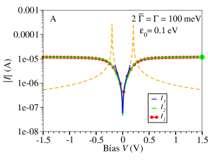
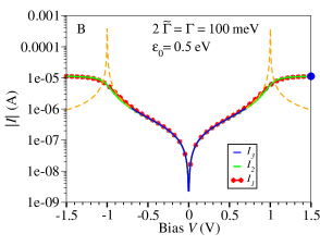
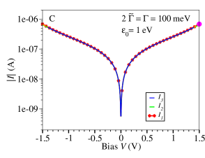
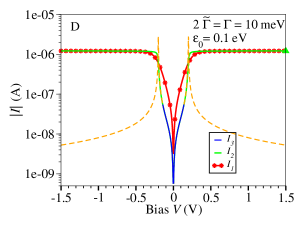
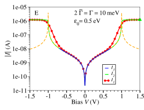
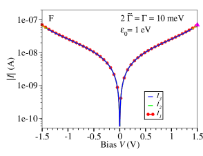
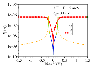
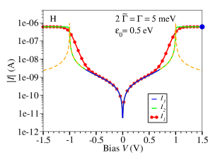
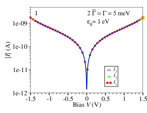
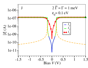
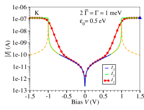
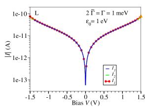
Fig.  1: Currents $I_{1}$, $I_{2}$, and $I_{3}$ computed using the parameters of Fig. 2 of Opodi et al.. Redrawing their figure emphasizes the difference between the current $I_{3}$ in the bias range for which eqn (3) was theoretically deduced ² (blue curves) and $I_{3}$ computed outside of bias range (orange dashed curves), wherein eqn (3) is merely a mathematical formula without any physical sense. Notice that, throughout, the green ($I_{2}$) and blue ($I_{3}$) curves excellently agree with the exact red curves ($I_{1}$) precisely in the parameter ranges predicted by theory, i.e. eqn (6) and eqn (12a). The tick symbols at $V=1.5$ V depicted in all panels emphasize that method 2 is very accurate, invalidating thereby the “applicability map” shown by Opodi et al. in their Fig. 5 (also reproduced in the present Fig. 2a).

To claim (ii):

Refuting claim (ii₁) is straightforward. Based on their Fig. 5, Opodi et al. cannot make a statement on method 3: they consider parameters $\varepsilon_{0}<1$ eV at the bias $V=1.5$ V($>1.4\,\left|\varepsilon_{0}\right|$), which is incompatible with eqn (12a). Noteworthily, the condition expressed by eqn (12a) defied by ref 1 was clearly stated in references that Opodi et al. have cited.

To reject claim (ii₂), I show in Fig. 2b, c, and d deviations of the current $I_{2}$ from the exact value $I_{1}$ in snapshots taken horizontally (i.e., constant $\Gamma$) and vertically (i.e., constant $\varepsilon_{0}$) across the “applicability map” (cf. Fig. 2a). As visible in Fig. 2b and c, in all regions where Opodi et al. claimed that method 2 is invalid the contrary is true; the largest relative deviation $I_{2}/I_{1}-1$ does not exceed 3%.

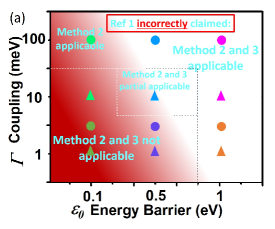
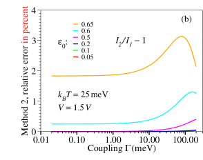
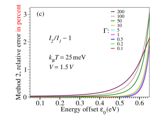
Fig.  2: (a) Tick symbols depicting excellent agreement between $I_{2}$ and $I_{1}$ in all panels of Fig. 1 overimposed on the “applicability map” adapted after Fig. 5 (courtesy Xi Yu) of ref. 1 contradict the claim of Opodi et al. on the inaplicability of method 2. (b,c) Deviations of $I_{2}$ from the exact current $I_{1}$ reveal that method 2 excellently works in situations where Opodi et al claimed the contrary. Importantly, showing parameter values $\left|\varepsilon_{0}\right|<1$ eV at bias $V=1.5$ V, panel a is beyond the scope of method 3 (cf. eqn (12a)).

What the physical quantity is underlying the color code depicted in their Fig. 5 (reproduced here in Fig. 2a) is not explained by Opodi et al. Anyway, the conclusion of Opodi et al. summarized in their Fig. 5 contradicts their results shown in their Fig. 2; all panels of that figure reveal excellent agreement between the green ($I_{2}$) and red (exact $I_{1}$) curves at $V=1.5$ V. For the reader’s convenience, the thick symbols at $V=1.5$ V in the present Fig. 1 overlapped on the “applicability map”of ref 1 emphasize this aspect. Inspection of these symbols (indicating that method 2 is excellent) overimposed on Fig. 2a reveals that they (also) lie in regions where Opodi et al. claimed that method 2 fails. Once more, their “applicability map” is factually incorrect.

To claim (iii): In their Fig. 3, 4A, 4B, S1 to S4, and S8 as well as in Table 2 Opodi et al. made unsuitable comparisons: the values for the CP-AFM junctions taken from their ref 38, 39, 44, and 57 (present ref 14, 4, 5, 15) are values of $\tilde{\Gamma}=\Gamma/2$, while those estimated by themselves are values of $\Gamma=2\tilde{\Gamma}$. Confusing $\tilde{\Gamma}$ and $\Gamma$, no wonder that they needed re-fitting of the original $I$-$V$ data. If they had correctly re-fitted the CP-AFM data using $I_{3}$, with all the values of $N$ given in the original works (namely, their ref 38, 39, 44, and 57, the present ref 14, 4, 5, 15), up to minor inaccuracies inherently arising from digitizing the experimental $I$-$V$-curves, they would have reconfirmed the values of $\varepsilon_{0}$ reported in the original publications, and would have obtained values of $\Gamma=2\tilde{\Gamma}$ two times larger than those originally reported for $\tilde{\Gamma}$ (cf. eqn (5)).

I still have to emphasize a difference of paramount importance between $I$-$V$ data fitting based on eqn (1) and (2) on one side, and eqn (3) on the other side. Eqn (1) and (2) have three independent fitting parameters $\left(\varepsilon_{0},N\Gamma_{g}^{2},\Gamma_{a}\right)\to\left(\left|\varepsilon_{0}\right|,N{\Gamma}^{2},{\Gamma}\right)$ while eqn (3) has only two independent fitting parameters $\left(\left|\varepsilon_{0}\right|,N\Gamma_{g}^{2}\right)\to\left(\left|\varepsilon_{0}\right|,N{\Gamma}^{2}\right)$.

All the narrative on the $N$-$\Gamma$-entanglement and wording on “twin sisters” used in Sec. 3.4 of the original article clearly reveal that ref. 1 overlooked that, when using $I_{3}$, $N$ and $\Gamma$ are two parameters whose values are impossible to separate; they build a unique fitting parameter $N{\Gamma}^{2}\equiv 4N\tilde{\Gamma}^{2}$. Data fitting using $I_{3}$ and three fitting parameters $\left(\varepsilon_{0},\Gamma,N\right)$ has an infinity number of solutions for $\Gamma$ and $N$ but they all yield a unique value of $N{\Gamma}^{2}$.

Were method 3 “quite limited” and the deviations of $I_{3}$ from $I_{1}$ or $I_{2}$ significant, Opodi et al. would have been able to determine three best fit parameters $\left(\left|\varepsilon_{0}\right|,\Gamma,N\right)$; at least for the “most problematic” junctions where they claimed important departures of $I_{3}$-based estimates from those based on $I_{1}$ and $I_{2}$. If this is indeed the case, the value of $N$ can be determined from data fitting ¹⁰. Their MATLAB code (additionally relevant details in the ESI) clearly reveals how they arrived at showing such differences for real junctions considered. In that code, they keep $N$ fixed and adjust $\varepsilon_{0}$ and $\Gamma$. As long it is reasonably realistic, an arbitrarily chosen value of $N$ has no impact on directly measurable properties. It changes the value of $\Gamma$ but neither $N\Gamma^{2}\propto G_{3}\approx G$ nor the level offset $\varepsilon_{0}$ changes, because method 3 performs well in almost all real cases.

However, defying available values of $N$ for the CP-AFM junctions to which they referred, Opodi et al. spoke of values up to $N\sim 10^{5}$. Employing such artificially large $N$’s nonphysically reduces $\Gamma$ ($N\Gamma^{2}\approx\mbox{constant}$, $\Gamma\propto 1/\sqrt{N}$) down to values incompatible with eqn (6b), arriving thereby at the idea that eqn (3) no longer applies.

In spot checks, I also interrogated curves shown by Opodi et al. for single-molecule mechanically controllable break junctions. I arrived so at the junction of 4,4’-bisnitrotolane (BNT),¹⁶ the real junction for which they claimed the most severe failure of method 3. If Fig. S7D to S7F and 4D of ref. 1 were correct, both $\varepsilon_{0}$ and $\Gamma$ based on $I_{3}$ would be in error by a factor of two.

To reject this claim, in Fig. 3 I show curves for $I_{1}$, $I_{2}$, and $I_{3}$ computed with the values of $\varepsilon_{0}$ and $\Gamma$ indicated by Opodi et al. in their Fig. S7D, E, and F, respectively. They should coincide with the black curves of Fig. S7D, E, and F, respectively if the latter were correct. According to Opodi et al., all these would represent fitting curves of the same experimental curve (red points in Fig. S7D, E, and F).

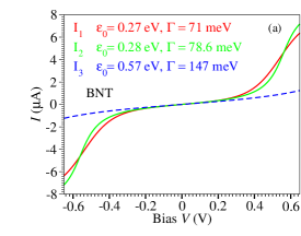
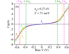
Fig.  3: (a) $I$-$V$ curves for single-molecule junctions ¹⁶ obtained using $N=1$ and parameters taken from the figures of ref. 1 indicated in the legends. To convince himself or herself that the present curves for $I_{2}$ and $I_{3}$ are correct and different from those of Fig. S7E and S7E of ref. 1, the reader can easily generate the present green and blue curves by using the GNUPLOT script of the ESI^†. (b) The curves for $I_{1}$, $I_{2}$, and $I_{3}$ computed with the parameter values (indicated in the inset) taken from Fig. S7D of ref. 1 do not support the failure of method 3 claimed by Opodi et al.

Provided that MATLAB is available, the reader can run the code “generateIVfitIV.m” included in the ESI^† to convince himself or herself that the red curve of Fig. 3a and not the black curve of Fig. S7D represents the exact current $I_{1}$ computed using eqn (1). Otherwise, running the GNUPLOT script also put in the ESI^† will at least convince the reader that the green and the blue lines of this figure and not the black curves in Fig. S7E and F, respectively do represent the currents $I_{2}$ and $I_{3}$ computed using eqn (2) and (3) for the parameters and the bias range indicated. The reader will realize that the three curves shown in Fig. 3 cannot represent best fits of the same experimental $I$-$V$-curve (red points in Fig. S7D, E, and F of ref 1).

If Opodi et al. had calculated $I_{2}$ and $I_{3}$ using the parameters indicated in their Fig. S7D, E, and F (same as in the present Fig. 3a), they would not have obtained the black curves of their Fig. S7D, E, and F but the red, green, and blue curves of Fig. 3a. The values $\varepsilon_{0}=0.57$ eV and $\Gamma=147$ meV of Fig. S7F (so much different from $\varepsilon_{0}=0.27$ eV and $\Gamma=71$ meV of Fig. S7D and $\varepsilon_{0}=0.28$ eV and $\Gamma=78.6$ meV of Fig. S7E) can by no means be substantiated from these calculations. All aforementioned values of $\varepsilon_{0}$ and $\Gamma$ of Fig. S7D, E, and F are exactly the same as the values shown in Table 2 and Fig. 4D of ref 1, and used as argument against method 3.

As additional support, I also show (Fig. 3b) the curves for $I_{1}$, $I_{2}$, and $I_{3}$, all computed with the same parameters, namely those of Fig. S7D of ref 1 ($\varepsilon_{0}=0.27$ eV and $\Gamma=71$ meV). In accord with the general theoretical considerations presented under (b) and (c), the differences between $I_{2}$ and $I_{3}$ (blue and green curves) are negligible, while deviations of $I_{2}$ from $I_{1}$ are notable only for biases close $\pm 2\varepsilon_{0}$ that invalidate eqn (6a).

To sum up, the claim of Opodi et al. on the failure of method 3 for the specific case considered above is incorrect because is based on values incompatible with calculations.

As made clear under (c) above, eqn (12a) is a condition deduced analytically. If it holds, eqn (3) is within $\sim 1\%$ as good as eqn (2). It makes little sense to check numerically a general condition deduced analytically, or even worse (as done in ref. 1) to claim that it does not apply for biases incompatible with eqn (12a).

The interested scholar needs not the “applicability map” (Fig. 5 of ref 1, to be corrected elsewhere (I. Bâldea, to be submitted)). In the whole parameter ranges where Opodi et al. claimed the opposite, method 2 turned out to be extremely accurate (cf. Fig. 2b and c). Likewise, “by definition” (cf. eqn (12a)), method 3 should not be applied at biases above $eV>2\left|\varepsilon_{0}\right|$ shown there, which makes the “applicability map” irrelevant for method 3.

Theory should clearly indicate the parameter ranges where an analytic formula is valid. This is a task accomplished in case of eqn (3). In publications also cited by Opodi et al. ^{3, 11}, particular attention has been drawn on not to apply eqn (3) at biases violating eqn (12a)³ and/or for energy offsets ($\left|\varepsilon_{0}\right|\raisebox{-1.29167pt}{$\stackrel{{\scriptstyle<}}{{\sim}}$}0.5$ eV) where thermal effects ($k_{B}T\simeq 25\,\mbox{meV}\neq 0$) matter ¹¹. It is experimentalists’ responsibility not to apply it under conditions that defy the boundaries under which it was theoretically deduced.

Financial support from the German Research Foundation (DFG Grant No. BA 1799/3-2) in the initial stage of this work and computational support by the state of Baden-Württemberg through bwHPC and the German Research Foundation through Grant No. INST 40/575-1 FUGG (bwUniCluster 2.0, bwForCluster/MLS&WISO 2.0/HELIX, and JUSTUS 2.0 cluster) are gratefully acknowledged.

4:

5:

6:

7:

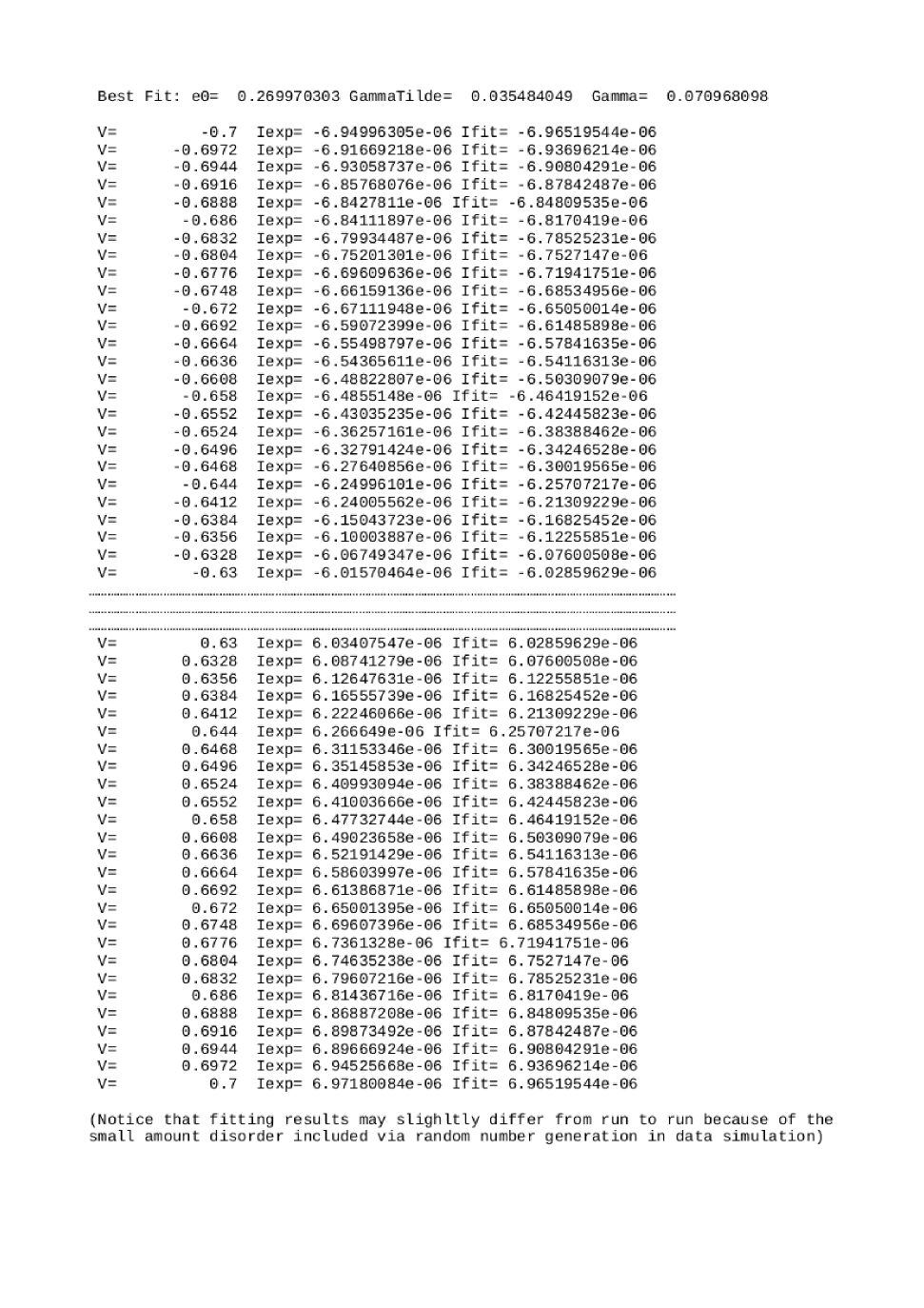
8: