Polynomiality of surface braid and mapping class group representations

Abstract

We study a wide range of homologically-defined representations of surface braid groups and of mapping class groups of surfaces, extending the Lawrence-Bigelow representations of the classical braid groups. These representations naturally come in families, defined either on all surface braid groups as the number of strands varies or on all mapping class groups as the genus varies. We prove that each of these families of representations is polynomial. This has applications to twisted homological stability as well as to understanding the structure of the representation theory of these families of groups. Our polynomiality result is a consequence of a more fundamental result establishing relations amongst the families of representations that we consider via short exact sequences of functors. As well as polynomiality, these short exact sequences also have applications to understanding the kernels of the homological representations under consideration.

Introduction

The representation theory of surface braid groups and of mapping class groups has been the subject of intensive study for several decades, and continues to be so; see for example the survey of Birman and Brendle [BB05, §4] or the expository article of Margalit [Mar19]. These groups naturally come in families – we will consider the following ones (where all surfaces are assumed connected, compact and with one boundary-component): the family of surface braid groups $\mathbf{B}_{n}(S)$ for each fixed surface $S$, as well as the two families $\mathbf{\Gamma}_{g,1}$ and $\boldsymbol{\mathcal{N}}_{h,1}$ of the mapping class groups of orientable and non-orientable surfaces respectively.

One way to make the representation theory of these groups more tractable is to study families of representations of each family of groups. Here, a family of representations means a collection of one representation of each group in the family so that the whole collection of representations is compatible, in a certain sense, with the natural homomorphisms between the groups. This structure is encoded by a functor $\langle\mathcal{G},\mathcal{M}\rangle\to R{}\textrm{-}\mathrm{Mod}$, where $\langle\mathcal{G},\mathcal{M}\rangle$ is a certain category whose automorphism groups are the family of groups in question. The richer structure of this category beyond its automorphism groups gives rise to the notion of polynomiality of functors $\langle\mathcal{G},\mathcal{M}\rangle\to R{}\textrm{-}\mathrm{Mod}$. This notion provides a way to organise and to understand more finely the structure of the representation theory of these families of groups. Moreover, polynomiality of such a functor implies, by the main result of Randal-Williams and Wahl [RW17], twisted homological stability for the family of groups with coefficients in the family of representations encoded by the functor.

The principal goal of this paper is to prove that a wide range of homologically-defined families of representations of surface braid groups and of mapping class groups are polynomial in this sense; see Corollary C. This is a consequence of our main result, Theorem B, which establishes fundamental short exact sequences relating different homological representation functors. This in turn depends on an initial study of the underyling module structure of these representations; see Theorem A. The short exact sequences that we construct also have further corollaries, concerning the kernels of homological representations (Corollaries E and F) and analyticity of quantum braid group representations (Corollary G).

Families of representations.

The families of representations of surface braid groups and of mapping class groups that we study in this paper are constructed systematically from natural actions on the homology of configuration spaces on the underlying surface, with coefficients twisted by certain local systems on these configuration spaces. Special cases of this construction recover, for example, the Lawrence-Bigelow representations of the classical braid groups [Law90, Big04] (Example 1.11), the An-Ko representations of surface braid groups [AK10] (Example 1.13) and the Moriyama representations of mapping class groups [Mor07] Example 1.16). In general, our construction depends on a choice of an ordered partition $\mathbf{k}$ of a positive integer $k$, corresponding to the number and partition of points in the configuration space, together with a non-negative integer $\ell$, which determines the local system via a lower central series, and produces a functor

$$\mathfrak{L}_{(\mathbf{k},\ell)}\colon\langle\mathcal{G},\mathcal{M}\rangle\longrightarrow R{}\textrm{-}\mathrm{Mod}.$$ (0.1)

This construction (together with some variants) is described in detail in §1.2, where we also explain how it fits into the larger framework of [PS21]. The objects of $\langle\mathcal{G},\mathcal{M}\rangle$ are indexed by non-negative integers $\mathtt{n}$ whose automorphism group is either $\mathbf{B}_{n}(S)$, $\mathbf{\Gamma}_{n,1}$ or $\boldsymbol{\mathcal{N}}_{n,1}$, depending on the context.

We mention for the sake of accuracy that the target category of (0.1) must in general be enlarged to the category $R{}\textrm{-}\mathrm{Mod}^{\mathrm{tw}}$ of twisted $R$-modules: this has the same objects as $R{}\textrm{-}\mathrm{Mod}$ but morphisms are permitted to act on the underlying ring $R$ as well as on the modules (see §1.2.2). We will elide this subtlety in the introduction, although we are careful in the rest of the paper about when the target is $R{}\textrm{-}\mathrm{Mod}^{\mathrm{tw}}$ and when we may restrict to $R{}\textrm{-}\mathrm{Mod}$. (One may always compose with the functor $R{}\textrm{-}\mathrm{Mod}^{\mathrm{tw}}\to\mathbb{Z}{}\textrm{-}\mathrm{Mod}$ that forgets module structures to avoid this twisting.)

Notation.

When we are not working in a specific setting, we denote the functors that we construct by $\mathfrak{L}_{(\mathbf{k},\ell)}$, as in (0.1) above. When we are working in the setting of surface braid groups on a fixed surface $S$, we write $\mathfrak{L}_{(\mathbf{k},\ell)}=\mathfrak{L}_{(\mathbf{k},\ell)}(S)$. In the special case of classical braid groups ($S=\mathbb{D}$) we also write $\mathfrak{L}_{(\mathbf{k},\ell)}(\mathbb{D})=\mathfrak{LB}_{(\mathbf{k},\ell)}$, since they extend the $\mathfrak{L}$awrence-$\mathfrak{B}$igelow representations. In the setting of mapping class groups of orientable surfaces, we write $\mathfrak{L}_{(\mathbf{k},\ell)}=\mathfrak{L}_{(\mathbf{k},\ell)}(\mathbf{\Gamma})$; in the setting of mapping class groups of non-orientable surfaces, we write $\mathfrak{L}_{(\mathbf{k},\ell)}=\mathfrak{L}_{(\mathbf{k},\ell)}(\boldsymbol{\mathcal{N}})$.

Module structure.

As a first step, we study the structure of the underlying modules of our representations.

The underlying modules of our representations are all of the following form. Let $S$ be a compact, connected surface with one boundary component and let $A\subset S$ be either a finite subset of its interior or a point on its boundary. For a tuple $\mathbf{k}=(k_{1},\ldots,k_{r})$ of positive integers summing to $k$, we consider the $\mathbf{k}$-partitioned configuration space

$$C_{\mathbf{k}}(S\smallsetminus A)=\{(x_{1},\ldots,x_{k})\in(S\smallsetminus A)^{k}\mid x_{i}\neq x_{j}\text{ for }i\neq j\}/\mathfrak{S}_{\mathbf{k}},$$

where $\mathfrak{S}_{\mathbf{k}}=\mathfrak{S}_{k_{1}}\times\cdots\times\mathfrak{S}_{k_{r}}\subseteq\mathfrak{S}_{k}$. Let $\mathcal{L}$ be a local system on $C_{\mathbf{k}}(S\smallsetminus A)$, defined over a ring $R$, and denote its fibre by $V$. The underlying modules of our representations are given by the twisted Borel-Moore homology modules $H_{k}^{\mathrm{BM}}(C_{\mathbf{k}}(S\smallsetminus A);\mathcal{L})$.

Theorem A (Proposition 2.4)

The twisted Borel-Moore homology $H_{*}^{\mathrm{BM}}(C_{\mathbf{k}}(S\smallsetminus A);\mathcal{L})$ is trivial except in degree $k$. There is an isomorphism of $R$-modules

$$H_{k}^{\mathrm{BM}}(C_{\mathbf{k}}(S\smallsetminus A);\mathcal{L})\;\cong\;\bigoplus_{w}V,$$ (0.2)

where the direct sum on the right-hand side is indexed by the following combinatorial data. Let $\Gamma$ be an embedded graph in $S$ with set of vertices $A$, such that $S$ deformation retracts onto $\Gamma$ relative to $A$; see Figure 2.1 for illustrations. There is then one copy of $V$ in the direct sum for each function $w$ assigning to each edge of $\Gamma$ a word in the alphabet $\{1,\ldots,r\}$ so that each letter $i\in\{1,\ldots,r\}$ appears precisely $k_{i}$ times as $w$ runs over all edges of $\Gamma$.

In each of our examples, $\mathcal{L}$ will be a rank-$1$ local system, i.e. $V\cong R$, so Theorem A says that $H_{k}^{\mathrm{BM}}(C_{\mathbf{k}}(S\smallsetminus A);\mathcal{L})$ is a free $R$-module, with a free generating set given by the set of functions $w$ described above. We note that, in the special case when $\mathbf{k}=(k)$, the direct sum in (0.2) is indexed by functions $w$ assigning non-negative integers to each edge of $\Gamma$ that sum to $k$.

Remark 0.1

The principal reason why we work with Borel-Moore homology instead of ordinary homology is the structural result of Theorem A. In contrast, the ordinary (co)homology of configuration spaces on surfaces is in general much more complicated, and the few cases in which the computations are known lead to representations that are much harder to handle; see for instance [Sta23, Th. 1.4]. On the other hand, under a certain condition on the local system $\mathcal{L}$ (called “genericity”), the ordinary and Borel-Moore homology of configuration spaces on orientable surfaces with coefficients in $\mathcal{L}$ are naturally isomorphic. Over the field $R=\mathbb{C}$ this is due to [Koh17, Theorem 3.1]; see also [AP20, Proposition D] for an extension to more general ground rings.

Short exact sequences of functors.

Our main result proves the existence of fundamental short exact sequences relating various different homological representation functors. Our polynomiality results, as well as results establishing other properties of these representations, are corollaries of these.

The short exact sequences depend on a “translation” operation $\tau_{\mathtt{1}}$ defined on functors (0.1), which is defined precisely in §3.1.1. For a tuple $\mathbf{k}=(k_{1},\ldots,k_{r})$ of positive integers, write $\mathbf{k}_{j}$ for the tuple obtained by subtracting $1$ from the $j$th term (and removing the $j$th term entirely, if it is now zero); see also Notation 3.2. In the setting of the classical braid groups (corresponding to $\mathcal{G}=\mathcal{M}=\boldsymbol{\beta}$), our result is the following.

Theorem B (Theorems 3.14, 3.19 and 3.27)

For any $\mathbf{k}=(k_{1},\ldots,k_{r})$ and $\ell$, there is a short exact sequence

(0.3)

of functors $\langle\boldsymbol{\beta},\boldsymbol{\beta}\rangle\to R{}\textrm{-}\mathrm{Mod}$. There are analogous short exact sequences of functors in the settings of surface braid groups – see (3.13) – and mapping class groups of surfaces –see (3.19) and (3.20). In the latter case, these short exact sequences are moreover split.

Polynomiality.

Our first corollary of Theorem B, and its analogues for surface braid groups and mapping class groups of surfaces, is that all of the functors (0.1) are polynomial in the sense recalled precisely in §4.1. Fix a positive integer $k$ and a tuple $\mathbf{k}=(k_{1},\ldots,k_{r})$ of positive integers summing to $k$, as well as a non-negative integer $\ell$.

Corollary C

In the setting of the classical braid groups:

• The functor $\mathfrak{LB}_{((1),\ell)}$ is strong polynomial of degree $2$ and weak polynomial of degree $1$.

• For $k\geqslant 2$, the functor $\mathfrak{LB}_{(\mathbf{k},\ell)}$ is very strong polynomial and weak polynomial of degree $k$.

In the setting of surface braid groups on $S=\Sigma_{g,1}\text{ or }\mathscr{N}_{h,1}$ for $g,h\geqslant 1$:

• The functor $\mathfrak{L}_{(\mathbf{k},\ell)}(S)$ is very strong polynomial and weak polynomial of degree $k$.

In the setting of mapping class groups of surfaces:

• The functors $\mathfrak{L}_{(\mathbf{k},\ell)}(\mathbf{\Gamma})$ and $\mathfrak{L}_{(\mathbf{k},\ell)}(\boldsymbol{\mathcal{N}})$ are split polynomial and weak polynomial of degree $k$.

In each setting, we also define an alternative version of each of the functors $\mathfrak{L}_{(\mathbf{k},\ell)}$, which we call its “vertical-type alternative” functor (this terminology refers to the shape of the homology cycles representing a basis for the underlying modules of these alternative representations; see Figure 2.3) and denote by $\mathfrak{L}^{v}_{(\mathbf{k},\ell)}$. In general, these functors have very different polynomiality behaviour:

Theorem D

In the setting of the classical braid groups:

• The functor $\mathfrak{LB}^{v}_{(\mathbf{k},\ell)}$ is not strong polynomial, but it is weak polynomial of degree $0$.

In the setting of surface braid groups on $S=\Sigma_{g,1}\text{ or }\mathscr{N}_{h,1}$ for $g,h\geqslant 1$:

• The functor $\mathfrak{L}^{v}_{(\mathbf{k},\ell)}(S)$ is not strong polynomial, but it is weak polynomial of degree $0$.

In the setting of mapping class groups of surfaces:

• For $\ell\in\{1,2\}$, the functors $\mathfrak{L}^{v}_{(\mathbf{k},\ell)}(\mathbf{\Gamma})$ and $\mathfrak{L}^{v}_{(\mathbf{k},\ell)}(\boldsymbol{\mathcal{N}})$ are split polynomial and weak polynomial of degree $k$.

Corollary C and Theorem D are proven in §4.2 for the classical braid groups and surface braid groups and §4.3 for mapping class groups of surfaces. Closely related to the functors $\mathfrak{L}^{v}_{(\mathbf{k},\ell)}$ are certain other functors $\mathfrak{L}^{\vee}_{(\mathbf{k},\ell)}$, which on objects are given by the dual representations of the representations associated to the objects of $\mathfrak{L}_{(\mathbf{k},\ell)}$. See Remark 2.11 for the relation between these. The statement of Theorem D also holds for these functors, as we prove in Theorems 4.7 and 4.9.

Consequences of polynomiality.

Corollary C and Theorem D have immediate consequences for twisted homological stability of surface braid groups on $\Sigma_{g,1}$ or $\mathscr{N}_{h,1}$ and mapping class groups of orientable or non-orientable surfaces. In each of these settings, twisted homological stability holds with coefficients in any functor that is either very strong polynomial or split polynomial, by work of Randal-Williams and Wahl [RW17, Theorems D, 5.26 and I]. In the case of mapping class groups of orientable surfaces, this was also proven earlier by Ivanov [Iva93] and Boldsen [Bol12].

Functors (0.1) that are weak polynomial of degree at most $d$ form a category $\mathcal{P}ol_{d}(\langle\mathcal{G},\mathcal{M}\rangle)$ that is localising in $\mathcal{P}ol_{d+1}(\langle\mathcal{G},\mathcal{M}\rangle)$; see Proposition 4.2. This allows one to define a sequence of quotient categories

(0.4)

where each functor $\mathcal{P}_{d}$ is induced by the difference functor defined in §3.1.1. This provides an organising tool for families of representations. It follows from Corollary C that, in each of our settings, the functor $\mathfrak{L}_{(\mathbf{k},\ell)}$ is a non-trivial element of $\mathcal{P}ol_{k}(\langle\mathcal{G},\mathcal{M}\rangle)/\mathcal{P}ol_{k-1}(\langle\mathcal{G},\mathcal{M}\rangle)$. Moreover, for each partition $\mathbf{k}^{\prime}\vdash k-1$ obtained from $\mathbf{k}$ by subtracting $1$ in one partition block, the functor $\mathfrak{L}_{(\mathbf{k}^{\prime},\ell)}$ is a direct summand of $\mathcal{P}_{d}(\mathfrak{L}_{(\mathbf{k},\ell)})$.

Faithfulness.

A second application of the short exact sequence (0.3) of Theorem B is to deduce inclusions between the kernels of different homological representations. In the case of the classical braid groups, applying the celebrated result of Bigelow [Big01] and Krammer [Kra02] (in the form proven in [Big02, §4]) on the faithfulness of certain homological representations of the braid groups, we deduce that many other homological representations of the braid groups are also faithful.

For tuples $\mathbf{k}^{\prime}=(k^{\prime}_{1},\ldots,k^{\prime}_{s})$ and $\mathbf{k}=(k_{1},\ldots,k_{r})$, write $\mathbf{k}^{\prime}\prec\mathbf{k}$ if for each $1\leqslant i\leqslant s$ we have $k^{\prime}_{i}\leqslant k_{j_{i}}$ for $1\leqslant j_{1}<\cdots<j_{s}\leqslant r$. This is a partial ordering on tuples of positive integers.

Corollary E

Whenever $\mathbf{k}^{\prime}\prec\mathbf{k}$ and $\ell\geqslant 1$, we have an inclusion

$$\mathrm{ker}\bigl{(}\mathfrak{LB}_{(\mathbf{k},\ell)}(\mathtt{n}+1)\bigr{)}\subseteq\mathrm{ker}\bigl{(}\mathfrak{LB}_{(\mathbf{k}^{\prime},\ell)}(\mathtt{n}+1)\bigr{)}$$

of kernels of $\mathbf{B}_{n}$-representations.

We note that, by construction, these are representations of $\mathbf{B}_{n+1}$ that we are considering as representations of $\mathbf{B}_{n}$ by restriction.

Proof.

By Theorem B, there is an epimorphism of functors $\tau_{\mathtt{1}}\mathfrak{LB}_{(\mathbf{k},\ell)}\twoheadrightarrow\tau_{\mathtt{1}}\mathfrak{LB}_{(\mathbf{k}_{j},\ell)}$ for any $1\leqslant j\leqslant r$. Repeating this finitely many times, we therefore obtain an epimorphism $\tau_{\mathtt{1}}\mathfrak{LB}_{(\mathbf{k},\ell)}\twoheadrightarrow\tau_{\mathtt{1}}\mathfrak{LB}_{(\mathbf{k}^{\prime},\ell)}$. Restricting to the automorphism group of the object $\mathtt{n}$, we obtain a surjection of $\mathbf{B}_{n}$-representations $\mathfrak{LB}_{(\mathbf{k},\ell)}(\mathtt{n}+1)\twoheadrightarrow\mathfrak{LB}_{(\mathbf{k}^{\prime},\ell)}(\mathtt{n}+1)$, which implies the claimed inclusion of kernels. ∎

Analogous inclusions of kernels of representations of $\mathbf{B}_{n}(S)$, $\mathbf{\Gamma}_{g,1}$ and $\boldsymbol{\mathcal{N}}_{h,1}$ follow by the same reasoning from the short exact sequences (3.13), (3.19) and (3.20).

Corollary F

For any $\ell\geqslant 2$ and any tuple $\mathbf{k}=(k_{1},\ldots,k_{r})$ where $k_{i}\geqslant 2$ for at least one $1\leqslant i\leqslant r$, the $\mathbf{B}_{n}$-representation $\mathfrak{LB}_{(\mathbf{k},\ell)}(\mathtt{n}+1)$ is faithful.

Proof.

By hypothesis $(2)\prec\mathbf{k}$, so it suffices by Corollary E to prove that $\mathfrak{LB}_{((2),\ell)}(\mathtt{n}+1)$ is faithful as a $\mathbf{B}_{n}$-representation. For $\ell=2$, it is proven in [Big02, §4] (see also [Big01, Kra02]) that $\mathfrak{LB}_{((2),2)}(\mathtt{n}+1)$ is faithful as a $\mathbf{B}_{n+1}$-representation and hence, by restriction, also as a $\mathbf{B}_{n}$-representation. In [PS21, §5.2.1.2], it is explained how to deduce from this that $\mathfrak{LB}_{((2),\ell)}(\mathtt{n}+1)$ is faithful for all $\ell\geqslant 2$. ∎

Analyticity.

As a final application, we prove analyticity (and non-polynomiality) of a functor encoding certain quantum representations of the braid groups.

There is a representation $\mathbb{V}$ of $\mathbb{U}_{q}(\mathfrak{sl}_{2})$, the quantum enveloping algebra of the Lie algebra $\mathfrak{sl}_{2}$, defined over the ring $\mathbb{L}:=\mathbb{Z}[\mathfrak{s}^{\pm 1},\mathfrak{q}^{\pm 1}]$, introduced by Jackson and Kerler [JK11] and called the generic Verma module. The structure of $\mathbb{U}_{q}(\mathfrak{sl}_{2})$ as a quasitriangular Hopf algebra induces a $\mathbf{B}_{n}$-representation on its $n$th tensor power $\mathbb{V}^{\otimes n}$, which we call the $n$th Verma module representation.

Corollary G (Corollary 4.11)

There is a functor $\mathfrak{Ver}\colon\langle\boldsymbol{\beta},\boldsymbol{\beta}\rangle\to\mathbb{L}{}\textrm{-}\mathrm{Mod}$ whose restriction to the automorphism group of $\mathtt{n}$ is the $n$th Verma module representation. Moreover, this functor is analytic, i.e. a colimit of polynomial functors, but it is not polynomial.

Remark 0.2

Theorem D and Corollary G illustrate that polynomiality is not an “automatic” property of families of representations, even in cases (such as the first two points of Theorem D) where the dimensions of the underlying modules of the representations grow polynomially with $\mathtt{n}$. See also Remark 4.12 for more examples of non-polynomial families of representations.

Outline.

In §1, we explain the categorical framework for families of groups that we work with (§1.1), construct the functors (0.1) in this framework (§1.2) and then discuss this construction in more detail (§1.3) in each of our three settings: classical braid groups, surface braid groups and mapping class groups of surfaces. In §2, we study the underlying module structure of these representations, proving Theorem A. In §3 we then construct the short exact sequences of Theorem B, recalling first the necessary background on translation, difference and evanescence operations on functors (§3.1). Finally, in §4 we prove our results on polynomiality (Corollary C and Theorem D) and analyticity (Corollary G).

General notation.

We denote by $\mathbb{N}$ the set of non-negative integers. For a small category $\mathcal{C}$, we use the abbreviation $\mathrm{ob}(\mathcal{C})$ to denote the set of objects of $\mathcal{C}$. For $\mathcal{D}$ any category and $\mathcal{C}$ a small category, we denote by $\mathbf{Fct}(\mathcal{C},\mathcal{D})$ the category of functors from $\mathcal{C}$ to $\mathcal{D}$. For $X$ a manifold with boundary, $\mathring{X}$ denotes its interior. For $R$ a non-zero unital ring, we denote by ${R}{}\textrm{-}\mathrm{Mod}$ the category of left $R$-modules. For an $R$-module $M$, we denote by $\mathrm{Aut}_{R}(M)$ the group of $R$-module automorphisms of $M$. When $R=\mathbb{Z}$, we omit it from the notation as long as there is no ambiguity. We denote by $\mathfrak{S}_{n}$ the symmetric group on a set of $n$ elements. For an integer $n\geqslant 1$, an ordered partition of $n$ means an ordered $r$-tuple $\mathbf{n}=\boldsymbol{\{}n_{1},...,n_{r}\boldsymbol{\}}$ of integers $n_{i}\geqslant 1$ (for some $r\geqslant 1$ called the length of $\mathbf{n}$) such that $n=\sum_{1\leqslant i\leqslant r}n_{i}$ (and without the condition $n_{i}\geqslant n_{i+1}$). The lower central series of a group $G$ is the descending chain of subgroups $\{\varGamma_{l}(G)\}_{l\geqslant 1}$ defined by $\varGamma_{1}(G):=G$ and $\varGamma_{l+1}(G):=[G,\varGamma_{l}(G)]$, the subgroup of $G$ generated by the commutators $[g,h]$ for $g\in G$ and $h\in\varGamma_{l}(G)$.

Acknowledgements.

The authors would like to thank Tara Brendle, Brendan Owens, Geoffrey Powell, Oscar Randal-Williams and Christine Vespa for illuminating discussions and questions. They would also like to thank Oscar Randal-Williams for inviting the first author to the University of Cambridge in November 2019, where the authors were able to make significant progress on the present article. In addition, they would like to thank Geoffrey Powell for a careful reading and many valuable comments on an earlier draft of this article. The first author was partially supported by a grant of the Romanian Ministry of Education and Research, CNCS - UEFISCDI, project number PN-III-P4-ID-PCE-2020-2798, within PNCDI III. The second author was supported by the Institute for Basic Science IBS-R003-D1, by a Rankin-Sneddon Research Fellowship of the University of Glasgow and by the ANR Project AlMaRe ANR-19-CE40-0001-01. The authors were able to make significant progress on the present article thanks to research visits to Glasgow and Bucharest, funded respectively by the School of Mathematics and Statistics of the University of Glasgow and the above-mentioned grant PN-III-P4-ID-PCE-2020-2798.

Contents

1. 1 Background
   1. 1.1 Categorical framework for families of groups
   2. 1.2 Construction of homological representation functors
   3. 1.3 Applications for surface braid groups and mapping class groups
2. 2 Module structure
   1. 2.1 An isomorphism criterion for twisted Borel-Moore homology
   2. 2.2 Free bases
   3. 2.3 Dual bases
3. 3 Short exact sequences
   1. 3.1 Background and preliminaries
   2. 3.2 For surface braid group functors
   3. 3.3 For mapping class group functors
4. 4 Polynomiality
   1. 4.1 Notions of polynomiality
   2. 4.2 For surface braid group functors
   3. 4.3 For mapping class group functors
   4. 4.4 Analyticity of a quantum representation

1 Background

This section recollects the construction of homological representation functors introduced in [PS21]; see §1.2. We first recall the underlying categorical framework in §1.1 and then detail in §1.3 the outputs of the construction of [PS21] for the families of groups studied in this paper.

1.1 Categorical framework for families of groups

We introduce here the categorical framework that is central to this paper to handle families of groups. A reader familiar with [RW17] may skip this subsection.

Preliminaries on categorical tools.

We refer to [Mac98] for a complete introduction to the notions of strict monoidal categories and modules over them. We generically denote a strict monoidal category by $(\mathcal{C},\natural,\mathtt{0})$, where $\mathcal{C}$ is a category, $\natural$ is the monoidal product and $\mathtt{0}$ is the monoidal unit. If it is braided, then its braiding is denoted by $b_{A,B}^{\mathcal{C}}\colon A\natural B\overset{\sim}{\to}B\natural A$ for all objects $A$ and $B$ of $\mathcal{C}$. A left-module $(\mathcal{M},\natural)$ over a (strict) monoidal category $(\mathcal{C},\natural,\mathtt{0})$ is a category $\mathcal{M}$ with a functor $\natural\colon\mathcal{C}\times\mathcal{M}\to\mathcal{M}$ that is unital and associative. For instance, a monoidal category $(\mathcal{C},\natural,\mathtt{0})$ is equipped with a (strict) left-module structure over itself, induced by its monoidal product.

Considering the category of (small skeletal strict) braided monoidal groupoids $\mathfrak{BrG}$, there is always an arbitrary binary choice for the convention of the braiding. We may pass from one to the other by the following inversion of the braiding operator. Let $(-)^{\dagger}\colon\mathfrak{BrG}\to\mathfrak{BrG}$ be the endofunctor defined on each object $(\mathcal{G},\natural,\mathtt{0})$ by $(\mathcal{G},\natural,\mathtt{0})^{\dagger}=(\mathcal{G},\natural,\mathtt{0})$ as a monoidal groupoid but whose braiding is defined by the inverse of that of $(\mathcal{G},\natural,\mathtt{0})$, i.e. $b^{\mathcal{G}^{\dagger}}_{A,B}:=(b^{\mathcal{G}}_{B,A})^{-1}$.

1.1.1 The Quillen bracket construction

In this section, we describe a useful categorical construction to encode families of groups: the bracket construction due to Quillen, which is a particular case of a more general construction described in [Gra76, p.219]; see also [RW17, §1]. Throughout §1, we fix an object $(\mathcal{G},\natural,\mathtt{0})$ of $\mathfrak{BrG}$ and a (small strict) left-module $(\mathcal{M},\natural)$ over $\mathcal{G}$.

The Quillen bracket construction $\langle\mathcal{G},\mathcal{M}\rangle$ on the left-module $(\mathcal{M},\natural)$ over the groupoid $(\mathcal{G},\natural,\mathtt{0})$ is the category with the same objects as $\mathcal{M}$ and whose morphisms are given by:

$$\mathrm{Hom}_{\langle\mathcal{G},\mathcal{M}\rangle}(X,Y)=\underset{\mathcal{G}}{\mathrm{colim}}[\mathrm{Hom}_{\mathcal{M}}(-\natural X,Y)].$$

Thus, a morphism from $X$ to $Y$ in $\langle\mathcal{G},\mathcal{M}\rangle$ is an equivalence class of pairs $(A,\varphi)$, denoted by $[A,\varphi]\colon X\to Y$, where $A$ is an object of $\mathcal{G}$ and $\varphi\colon A\natural X\to Y$ is a morphism in $\mathcal{M}$. Also, for two morphisms $[A,\varphi]\colon X\to Y$ and $[B,\psi]\colon Y\to Z$ in $\langle\mathcal{G},\mathcal{M}\rangle$, the composition is defined by $[B,\psi]\circ[A,\varphi]=[B\natural A,\psi\circ(\mathrm{id}_{B}\natural\varphi)]$.

There is a faithful canonical functor $\mathcal{M}\hookrightarrow\langle\mathcal{G},\mathcal{M}\rangle$ defined as the identity on objects and sending $f\in\mathrm{Hom}_{\mathcal{M}}(X,Y)$ to $[\mathtt{0},f]$. From now on, we assume that $\mathcal{M}$ is a groupoid, that $(\mathcal{G},\natural,\mathtt{0})$ has no zero divisors (i.e. $A\natural B\cong\mathtt{0}$ if and only if $A\cong B\cong\mathtt{0}$ for $A,B\in\mathrm{Obj}(\mathcal{G})$) and that $\mathrm{Aut}_{\mathcal{G}}(\mathtt{0})=\{\mathrm{id}_{\mathtt{0}}\}$. These are properties that are satisfied in all the situations of this paper; see §1.1.2. Then $\mathcal{M}$ is the maximal subgroupoid of $\langle\mathcal{G},\mathcal{M}\rangle$ and, as an element of $\mathrm{Hom}_{\langle\mathcal{G},\mathcal{M}\rangle}(X,X)$, we abuse notation and write $f$ for $[\mathtt{0},f]$ for each $X\in\mathrm{Obj}(\mathcal{M})$ and $f\in\mathrm{Aut}_{\mathcal{G}}(X)$; see [RW17, Prop. 1.7].

Module structure.

The following discussion is a direct generalisation of [RW17, Prop. 1.8] to which we refer for further details. The category $\langle\mathcal{G},\mathcal{M}\rangle$ inherits a (strict) left-module structure over $(\mathcal{G},\natural,\mathtt{0})$ as follows. The module bifunctor $\natural$ extends to $\langle\mathcal{G},\mathcal{M}\rangle$ with the same assignment on objects, by letting, for $[X,\varphi]\in\mathrm{Hom}_{\langle\mathcal{G},\mathcal{M}\rangle}(A,B)$ and $[Y,\psi]\in\mathrm{Hom}_{\langle\mathcal{G},\mathcal{M}\rangle}(C,D)$:

$$\varphi\natural[Y,\psi]=[Y,(\varphi\natural\psi)\circ((b_{A,Y}^{\mathcal{G}})^{-1}\natural\mathrm{id}_{C})].$$ (1.1)

Extensions along the Quillen bracket construction.

The following result provides a way to extend a functor on the category $\mathcal{M}$ to a functor with $\langle\mathcal{G},\mathcal{M}\rangle$ as source category. Its proof repeats mutatis mutandis that of [Sou22, Lem. 1.2].

Lemma 1.1

Let $\mathcal{C}$ be a category and F an object of $\mathbf{Fct}(\mathcal{M},\mathcal{C})$. Assume that, for each $X\in\mathrm{Obj}(\mathcal{G})$ and $A\in\mathrm{Obj}(\mathcal{M})$, there exists a morphism $\alpha_{X,A}\colon F(A)\to F(X\natural A)$ such that $\alpha_{Y,X\natural A}\circ\alpha_{X,A}=\alpha_{Y\natural X,A}$ for all $Y\in\mathrm{Obj}(\mathcal{G})$ and $\alpha_{\mathtt{0},A}=\mathrm{id}_{F(A)}$. Then the assignments $F([X,\varphi])=F(\varphi)\circ\alpha_{X,A}$ to all morphisms $[X,\varphi]\colon A\to X\natural A$ of $\langle\mathcal{G},\mathcal{M}\rangle$ extend the functor $F\colon\mathcal{M}\to\mathcal{C}$ to a functor $F\colon\langle\mathcal{G},\mathcal{M}\rangle\to\mathcal{C}$ if and only if for all $X\in\mathrm{Obj}(\mathcal{G})$ and $A\in\mathrm{Obj}(\mathcal{M})$, for all $\varphi^{\prime}\in\mathrm{Aut}_{\mathcal{G}}(X)$ and $\varphi^{\prime\prime}\in\mathrm{Aut}_{\mathcal{M}}(A)$, the following relation holds:

$$F(\varphi^{\prime}\natural\varphi^{\prime\prime})\circ\alpha_{X,A}=\alpha_{X,A}\circ F(\varphi^{\prime\prime}).$$ (1.2)

Similarly, we may extend a morphism in $\mathbf{Fct}(\mathcal{M},\mathcal{C})$ to a morphism in $\mathbf{Fct}(\langle\mathcal{G},\mathcal{M}\rangle,\mathcal{C})$ thanks to the following result, whose proof repeats verbatim that of [Sou19, Lem. 1.12].

Lemma 1.2

Let $\mathcal{C}$ be a category, $F$ and $G$ objects of $\mathbf{Fct}(\langle\mathcal{G},\mathcal{M}\rangle,\mathcal{C})$ and $\eta\colon F\to G$ a natural transformation in $\mathbf{Fct}(\mathcal{M},\mathcal{C})$. The restriction $\mathbf{Fct}(\langle\mathcal{G},\mathcal{M}\rangle,\mathcal{C})\to\mathbf{Fct}(\mathcal{M},\mathcal{C})$ is obtained by precomposing by the canonical inclusion $\mathcal{M}\hookrightarrow\langle\mathcal{G},\mathcal{M}\rangle$. Then $\eta$ is a natural transformation in the category $\mathbf{Fct}(\langle\mathcal{G},\mathcal{M}\rangle,\mathcal{C})$ if and only if for all $A,B\in\mathrm{Ob}(\mathcal{M})$ such that $B\cong X\natural A$ with $X\in\mathrm{Ob}(\mathcal{G})$:

$$\eta_{B}\circ F([X,\mathrm{id}_{B}])=G([X,\mathrm{id}_{B}])\circ\eta_{A}.$$ (1.3)

1.1.2 Categories for surface braid groups and mapping class groups

We now recollect the suitable categories associated to the families of groups we study. The content of this section is classical knowledge; see [RW17, §5.6] (for the original definitions of the categories) and [Sou22, §3.1] (for the skeletal versions) for further technical justifications of the properties and definitions.

1.1.2.1 For mapping class groups of surfaces

The decorated surface groupoid $\hat{\mathcal{M}}_{2}$ is introduced in [RW17, §5.6] and defined as follows. Its objects are the decorated surfaces $\left(S,k,I\right)$, where $S$ is a smooth connected compact surface with one boundary component $\partial S$, with a finite set of $k\geqslant 0$ points removed from the interior of $S$ (in other words with punctures) together with a parametrised interval $I\colon[-1,1]\hookrightarrow\partial S$ in the boundary. When there is no ambiguity, we omit $k$ and $I$ from the notation for convenience. Let $\mathrm{Diff}_{I}(S,\mathbf{k})$ be the group of diffeomorphisms of the surface $\bar{S}$ obtained from $S$ by filling in each puncture with a marked point, which restrict to the identity on a neighbourhood of the parametrised interval $I$ and fixing the $k$ marked points setwise by stabilising the partition $\mathbf{k}$ as a subset. When the surface $S$ is orientable, the orientation on $S$ is induced by the orientation of $I$, and then the isotopy classes of $\mathrm{Diff}_{I}(S,\mathbf{k})$ automatically preserve that orientation. The (auto)morphisms of $\hat{\mathcal{M}}_{2}$ are the mapping class groups of $(S,\mathbf{k},I)$ denoted by $\mathrm{MCG}(S,\mathbf{k})$, i.e. the isotopy classes $\pi_{0}\mathrm{Diff}_{I}(S,\mathbf{k})$.

By [RW17, §5.6.1], the boundary connected sum $\natural$ induces a braided monoidal structure on $\hat{\mathcal{M}}_{2}$ as follows. For a parametrised interval $I$, the left half-interval $[-1,0]\hookrightarrow\partial S$ of $I$ is denoted by $I^{-}$ and the right half-interval $[0,1]\hookrightarrow\partial S$ of $I$ is denoted by $I^{+}$, so that $I=I^{-}\cup I^{+}$. For two decorated surfaces $(S_{1},I_{1})$ and $(S_{2},I_{2})$, the boundary connected sum $(S_{1},I_{1})\natural(S_{2},I_{2})$ is defined to be the surface $(S_{1}\natural S_{2},I_{1}\natural I_{2})$, where $S_{1}\natural S_{2}$ is obtained by gluing $S_{1}$ and $S_{2}$ along the half-interval $I_{1}^{+}$ and the half-interval $I_{2}^{-}$ and $I_{1}\natural I_{2}=I_{1}^{-}\cup I_{2}^{+}$. The braiding $b_{S_{1},S_{2}}^{\hat{\mathcal{M}}_{2}}$ of the monoidal structure is the half Dehn twist with respect to the separating curve $I_{2}^{-}=I_{1}^{+}$ that exchanges the two summands $S_{1}$ and $S_{2}$; see [RW17, Fig. 2] or Figure 3.6. In order to strictify this monoidal structure, we arbitrarily pick a surface that is homeomorphic to the $2$-disc, which is thus a monoidal unit $\mathtt{0}$ for $\hat{\mathcal{M}}_{2}$. We then apply [Sch01, Th. 4.3], which says that one may force the monoidal structure to be strict, without changing the underlying category or the unit object, by making careful choices of concrete (set-theoretic) realisations of $S_{1}\natural S_{2}$ for each $S_{1}$ and $S_{2}$. Let us denote the resulting strict braided monoidal groupoid by $(\mathcal{M}_{2},\natural,\mathtt{0},b_{-,-}^{\mathcal{M}_{2}})$.

Now we fix a once-punctured disc $\mathbb{D}_{1}$, a torus with one boundary component $\mathbb{T}$ and a Möbius strip $\mathbb{M}$. We will generally denote $\mathbb{D}_{1}^{\natural s}$ by $\mathbb{D}_{s}$ for concision. Let $\mathcal{M}_{2}^{+}$ and $\mathcal{M}_{2}^{-}$ be the full subgroupoids of $\mathcal{M}_{2}$ on the objects $\{\mathbb{T}^{\natural g}\}_{g\in\mathbb{N}}$ and $\{\mathbb{M}^{\natural h}\}_{h\in\mathbb{N}}$ respectively, where $\mathbb{T}^{\natural 0}=\mathbb{M}^{\natural 0}=\mathtt{0}$. The strict braided monoidal structure on $\mathcal{M}_{2}$ restricts to a strict braided monoidal structure on each of $\mathcal{M}_{2}^{+}$ and $\mathcal{M}_{2}^{-}$. We also note that these two subgroupoids are small, skeletal, have no zero divisors and that $\mathrm{Aut}_{\mathcal{M}_{2}^{+}}(\mathbb{T}^{\natural 0})=\mathrm{Aut}_{\mathcal{M}_{2}^{-}}(\mathbb{M}^{\natural 0})=\{id_{\mathtt{0}}\}$. We denote the mapping class groups $\mathrm{MCG}(\mathbb{T}^{\natural g})$ and $\mathrm{MCG}(\mathbb{M}^{\natural h})$ by $\mathbf{\Gamma}_{g,1}$ and $\boldsymbol{\mathcal{N}}_{h,1}$ respectively. In particular, we stress that the sets of objects $\mathrm{Obj}(\mathcal{M}_{2}^{+})$ and $\mathrm{Obj}(\mathcal{M}_{2}^{-})$ are both canonically isomorphic to the set of non-negative integers. Therefore, when there is no ambiguity or risk of confusion, we implicitly use these canonical identifications on the objects for the sake of simplicity, thus using the notation $\mathtt{n}$ to denote the surfaces $\mathbb{T}^{\natural n}$ or $\mathbb{M}^{\natural n}$.

1.1.2.2 For braid goups on surfaces

Let $S$ be a compact, connected, smooth surface with one boundary component. There exist integers $g\geqslant 0$ and $h\geqslant 0$ and a homeomorphism $S\cong\mathbb{T}^{\natural g}\natural\mathbb{M}^{\natural h}$ using the notations of §1.1.2.1. If the surface is orientable (i.e. $h=0$), then $g$ is unique and we prefer to denote $S\cong\mathbb{T}^{\natural g}$ by $\Sigma_{g,1}$. We also denote $S\cong\mathbb{M}^{\natural h}$ by $\mathscr{N}_{h,1}$. There are several ways to introduce (partitioned) surface braid groups; see for example [DPS22, §6.2–6.3] for a detailed overview. For a partition $\mathbf{n}=\boldsymbol{\{}n_{1},\ldots,n_{r}\boldsymbol{\}}\vdash n$, we denote by $C_{\mathbf{n}}(S)$ the $\mathbf{n}$-configuration space $\left\{\left(x_{1},\ldots,x_{n}\right)\in S^{\times n}\mid x_{i}\neq x_{j}\textrm{ if }i\neq j\right\}/\mathfrak{S}_{\mathbf{n}}$ of $n$ points in the surface $S$, with $\mathfrak{S}_{\mathbf{n}}:=\mathfrak{S}_{n_{1}}\times\cdots\times\mathfrak{S}_{n_{r}}$. The $\mathbf{n}$-partitioned braid group on $n$ strings on the surface $S$ is the fundamental group of this configuration space: $\mathbf{B}_{\mathbf{n}}(S)=\pi_{1}(C_{\mathbf{n}}(S),c_{0})$, where $c_{0}$ is a configuration in the boundary of $S$. The braid groups on the $2$-disc $\mathbb{D}$ are the classical braid groups; we omit $\mathbb{D}$ from the notation in this case. Full presentations of these groups are recalled in [PS23, Prop. 2.2].

The family of classical braid groups is associated with the small skeletal groupoid $\boldsymbol{\beta}$, with objects the non-negative integers denoted by $\mathtt{n}$, and morphisms $\mathrm{Hom}_{\boldsymbol{\beta}}(\mathtt{n},\mathtt{m})=\mathbf{B}_{n}$ if $\mathtt{n}=\mathtt{m}$ and the empty set otherwise. The composition of morphisms $\circ$ in the groupoid $\boldsymbol{\beta}$ corresponds to the group operation of the braid groups. We recall from [Mac98, Chapter XI, §4] that $\boldsymbol{\beta}$ has a canonical strict monoidal product $\natural\colon\boldsymbol{\beta}\times\boldsymbol{\beta}\to\boldsymbol{\beta}$ defined by the usual addition for the objects and laying two braids side by side for the morphisms. The object $\mathtt{0}$ is the unit of this monoidal product. The strict monoidal groupoid $(\boldsymbol{\beta},\natural,\mathtt{0})$ is braided: the braiding is defined for all $\mathtt{n},\mathtt{m}\in\mathrm{Obj}(\boldsymbol{\beta})$ such that $\mathtt{n}+\mathtt{m}\geqslant 2$ by $b_{\mathtt{n},\mathtt{m}}^{\boldsymbol{\beta}}=(\sigma_{m}\circ\cdots\circ\sigma_{2}\circ\sigma_{1})\circ\cdots\circ(\sigma_{n+m-1}\circ\cdots\circ\sigma_{n+1}\circ\sigma_{n})$, where each $\sigma_{i}$ denotes the $i$th Artin generator. We note that $(\boldsymbol{\beta},\natural,\mathtt{0})$ has no zero divisors and that $\mathrm{Aut}_{\boldsymbol{\beta}}(\mathtt{0})=\{\mathrm{id}_{\mathtt{0}}\}$. Finally, there is an evident strict monoidal isomorphism between $(\boldsymbol{\beta},\natural,\mathtt{0})$ and the full subgroupoid of $\mathcal{M}_{2}$ on the objects $\{\mathbb{D}_{n}\}_{n\in\mathbb{N}}$, which obviously upgrades to a (strict) braided monoidal isomorphism with the following convention on the Artin generators.

Convention 1.3

For each $n\in\mathbb{N}$, we consider the punctured disc $\mathbb{D}_{n}$ with the canonical ordering of the punctures from the left to the right (under the “bird’s eye” viewpoint). Following [RW17, Fig. 2], we choose each generator $\sigma_{i}$ to be the geometric braid that swaps anticlockwise the points $i$ and $i+1$; see Figure 4.1 for an illustration of $\sigma_{1}$.

Similarly, let $\boldsymbol{\beta}^{S}$ be the groupoid with the same objects as $\boldsymbol{\beta}$ and morphisms given by $\mathrm{Hom}_{\boldsymbol{\beta}^{S}}(\mathtt{n},\mathtt{m})=\mathbf{B}_{n}(S)$ if $\mathtt{n}=\mathtt{m}$ and the empty set otherwise. In particular, we note that $\boldsymbol{\beta}^{S}\cong\boldsymbol{\beta}$ for $S\cong\mathbb{D}$. For each surface $S$, there is a canonical strict left $\boldsymbol{\beta}$-module structure on $\boldsymbol{\beta}^{S}$: the associative, unital functor $\natural\colon\boldsymbol{\beta}\times\boldsymbol{\beta}^{S}\to\boldsymbol{\beta}^{S}$ is defined by addition on objects and, on morphisms, by the maps of configuration spaces $C_{n}(\mathbb{D})\times C_{m}(S)\to C_{n+m}(S)$ induced by a choice of homeomorphism $\mathbb{D}\natural S\cong S$ whose restriction to the right-hand summand is a self-embedding of $S$ that is isotopic to the identity.

1.2 Construction of homological representation functors

Here we introduce the construction, based on the general machinery of [PS21, §2, §5], of homological representation functors for surface braid groups and mapping class groups of surfaces. Namely, we take inspiration from the constructions of [PS21], but follow a more direct method (although equivalent in the end) to define the homological representations functors; see Remark 1.8.

1.2.1 Framework

Let $\mathcal{G}$ be one of the small strict braided monoidal groupoids $\{\mathcal{M}_{2}^{+},\mathcal{M}_{2}^{-},\boldsymbol{\beta}\}$ introduced in §1.1.2 along with any associated $\mathcal{G}$-module $\mathcal{M}$ defined there (typically $\mathcal{M}_{2}^{+}$, $\mathcal{M}_{2}^{-}$ or $\boldsymbol{\beta}^{S}$). We denote by $\{G_{n}\}_{n\in\mathbb{N}}$ the family of automorphism groups $\{\mathrm{Aut}_{\mathcal{M}}(\mathtt{n})\}_{\mathtt{n}\in\mathrm{Obj}(\mathcal{M})}$ encoded by $\mathcal{M}$. These come equipped with canonical injections induced by the $\mathcal{G}$-module structure $\mathrm{id}_{\mathtt{1}}\natural(-)_{n}\colon G_{n}\hookrightarrow G_{n+1}$. The first key ingredient to define homological representations is to find a family of spaces on which the family $\{G_{n}\}_{n\in\mathbb{N}}$ acts. In the case of surface braid groups, this will involve considering “partitioned versions” of the groups $G_{n}$, which we define in a general context:

Definition 1.4 (Partitioned groups.)

Let $\mathsf{G}_{k}$ be a group equipped with a surjection $\mathsf{s}_{k}\colon\mathsf{G}_{k}\twoheadrightarrow\mathfrak{S}_{k}$. Given a partition $\mathbf{k}=\boldsymbol{\{}k_{1},\ldots,k_{r}\boldsymbol{\}}\vdash k$, for $j\leqslant r$, we define $t_{j}:=\sum_{i\leqslant j}k_{i}$ (including $t_{0}=0$). Then the set $\{t_{j-1}+1,\ldots,t_{j}\}$ is referred to as the $j$th block of $\mathbf{k}$, and $k_{i}$ is called the size of the $i$th block. The preimage $\mathsf{G}_{\mathbf{k}}:=\mathsf{s}_{k}^{-1}(\mathfrak{S}_{\mathbf{k}})$ (where $\mathfrak{S}_{\mathbf{k}}:=\mathfrak{S}_{k_{1}}\times\cdots\times\mathfrak{S}_{k_{r}}$) is called the $\mathbf{k}$-partitioned version of $\mathsf{G}_{k}$. The extremal situations are the discrete partition $\mathbf{k}=\boldsymbol{\{}1,\ldots,1\boldsymbol{\}}$, which corresponds to the pure version of the group $\mathsf{G}_{k}$, and the trivial case $\mathbf{k}=(k)$, which is simply the group $\mathsf{G}_{k}$ itself. The group $\mathsf{G}_{\mathbf{k}}$ fits into the short exact sequence: $1\to\mathsf{G}_{\boldsymbol{\{}1,\ldots,1\boldsymbol{\}}}\to\mathsf{G}_{\mathbf{k}}\to\mathfrak{S}_{\mathbf{k}}\to 1$.

In all the situations addressed in this paper, the parameter $k$ corresponds to the motion of $k$ points, while the surjection corresponds to the permutations of these points. For the remainder of §1.2, we consider a partition $\mathbf{k}=\boldsymbol{\{}k_{1};\ldots;k_{r}\boldsymbol{\}}\vdash k$ of an integer $k\geqslant 1$. Furthermore, for each $n\in\mathbb{N}$, we consider the surface $\mathcal{S}_{n}$ defined from the object $\mathtt{n}\in\mathrm{Obj}(\mathcal{M})$ as follows:

• When $G_{n}=\mathbf{B}_{n}(S)$ (where $S=\Sigma_{g,1}\text{ or }\mathscr{N}_{h,1}$), we set $\mathcal{S}_{n}:=\mathbb{D}_{n}\natural S$ and $G_{k,n}:=\mathbf{B}_{k,n}(S)$ equipped with the evident surjection $\mathbf{B}_{k,n}(S)\twoheadrightarrow\mathfrak{S}_{k}$; thus $G_{\mathbf{k},n}=\mathbf{B}_{\mathbf{k},n}(S)$.

• When $G_{n}=\mathrm{MCG}(\mathscr{S}^{\natural n})$ (where $\mathscr{S}=\mathbb{T}\text{ or }\mathbb{M}$), we set $\mathcal{S}_{n}:=(\mathscr{S}^{\natural n})\smallsetminus{I^{\prime}}$ where $I^{\prime}\subsetneq I$ denotes the image of the closed subinterval $[-1/2,1/2]$ in the boundary $\partial\mathscr{S}^{\natural n}$ (see Remark 1.15 for a justification of this choice). We also set $G_{k,n}:=\mathrm{MCG}(\mathscr{S}^{\natural n},k)$ equipped with the evident surjection $\mathrm{MCG}(\mathscr{S}^{\natural n},k)\twoheadrightarrow\mathfrak{S}_{k}$; thus $G_{\mathbf{k},n}=\mathrm{MCG}(\mathscr{S}^{\natural n},\mathbf{k})$.

We denote by $C_{\mathbf{k}}(\mathcal{S}_{n})$ the configuration space of points $\left\{\left(x_{1},\ldots,x_{k}\right)\in\mathcal{S}_{n}^{\times k}\mid x_{i}\neq x_{j}\textrm{ if }i\neq j\right\}/\mathfrak{S}_{\mathbf{k}}$ associated to the partition $\mathbf{k}$ of $k$ points in the surface $\mathcal{S}_{n}$. In each case, there is a split short exact sequence

(1.4)

known as the Fadell-Neuwirth exact sequence if $G_{n}=\mathbf{B}_{n}(S)$ (see for instance [PS21, Prop. 4.15] or [DPS22, Prop. 6.15]) and as the Birman short exact sequence if $G_{n}=\mathrm{MCG}(\mathscr{S}^{\natural n})$ (see for instance [FM12, Lem. 4.16] or [PS21, Cor. 4.19, §5.1.3]). In the latter case, we note that the kernel is a priori equal to $\mathbf{B}_{\mathbf{k}}(\mathscr{S}^{\natural n})$, but removing an interval from the boundary of $\mathscr{S}^{\natural n}$ does not change its isotopy type and so $\mathbf{B}_{\mathbf{k}}(\mathscr{S}^{\natural n})$ is identified with $\mathbf{B}_{\mathbf{k}}(\mathscr{S}^{\natural n}\smallsetminus I^{\prime})=\mathbf{B}_{\mathbf{k}}(\mathcal{S}_{n})$. This short exact sequence provides an action (by conjugation) of $G_{n}$ on $\mathbf{B}_{\mathbf{k}}(\mathcal{S}_{n})$. We note in passing that, in the case $G_{n}=\mathbf{B}_{n}(S)$, the section of (1.4), denoted by $s_{(\mathbf{k},n)}$, is such that its composition with the canonical injection $G_{\mathbf{k},n}\hookrightarrow G_{k+n}$ is equal to $\mathrm{id}_{k}\natural(-)_{n}\colon G_{n}\hookrightarrow G_{k+n}$.

1.2.2 Twisted representations

Another preliminary is the recollection of the notion of twisted representations.

Definition 1.5 (Category of twisted modules.)

Let $\mathbb{A}$ be a non-zero associative unital ring and let $R$ be an associative unital $\mathbb{A}$-algebra. The category of twisted $R$-modules, denoted by $R{}\textrm{-}\mathrm{Mod}^{\mathrm{tw}}$, is defined as follows. An object of $R{}\textrm{-}\mathrm{Mod}^{\mathrm{tw}}$ is simply a left $R$-module $V$. A morphism $V\to V^{\prime}$ is an automorphism $\psi\in\mathrm{Aut}_{\mathbb{A}\textrm{-}\mathsf{Alg}}(R)$ of unital $\mathbb{A}$-algebras together with a morphism $\theta\colon V\to\psi^{*}(V^{\prime})$ of left $R$-modules.

We will henceforth set $\mathbb{A}=\mathbb{Z}$, so that $\mathbb{A}$-algebras are just rings. From §1.2.3 onwards, we will typically work with group rings $R=\mathbb{Z}[Q]$.

A functor $F\colon\langle\mathcal{G},\mathcal{M}\rangle\to R{}\textrm{-}\mathrm{Mod}^{\mathrm{tw}}$ encodes twisted $R$-representations. More precisely, at the level of group representations, it means that the action of $G_{n}$ on the corresponding $R$-module commutes with the $R$-module structure only up to a “twist”, i.e. an action $a_{n}\colon G_{n}\to\mathrm{Aut}_{\mathsf{Ring}}(R)$. When this action $a_{n}$ is trivial, we recover the classical notion of an $R$-representation (also called genuine $R$-representation) of the group $G_{n}$.

Furthermore, the module category $R{}\textrm{-}\mathrm{Mod}$ is by definition the subcategory of $R{}\textrm{-}\mathrm{Mod}^{\mathrm{tw}}$ on the same objects and those morphisms $(\psi,\theta)$ with $\psi=\mathrm{id}_{R}$, so there is a canonical embedding $R{}\textrm{-}\mathrm{Mod}\subset R{}\textrm{-}\mathrm{Mod}^{\mathrm{tw}}$. In particular, a representation encoded by a functor $F\colon\langle\mathcal{G},\mathcal{M}\rangle\to R{}\textrm{-}\mathrm{Mod}^{\mathrm{tw}}$ is a genuine $R$-representation if and only if $F$ factors through the module subcategory $R{}\textrm{-}\mathrm{Mod}$:

$$F\colon\langle\mathcal{G},\mathcal{M}\rangle\longrightarrow R{}\textrm{-}\mathrm{Mod}\lhook\joinrel\longrightarrow R{}\textrm{-}\mathrm{Mod}^{\mathrm{tw}}.$$ (1.5)

In any case, representations encoded by functors $\langle\mathcal{G},\mathcal{M}\rangle\to R{}\textrm{-}\mathrm{Mod}^{\mathrm{tw}}$ may always be viewed as genuine $\mathbb{Z}$-module representations. Indeed, there is a forgetful functor $R{}\textrm{-}\mathrm{Mod}^{\mathrm{tw}}\to{\mathbb{Z}}{}\textrm{-}\mathrm{Mod}$, where we forget the $R$-module structure on objects and the $\psi$ component of a morphism $(\psi,\theta)$ in Definition 1.5. Hence, we may always form the composite

$$\langle\mathcal{G},\mathcal{M}\rangle\longrightarrow R{}\textrm{-}\mathrm{Mod}^{\mathrm{tw}}\longrightarrow{\mathbb{Z}}{}\textrm{-}\mathrm{Mod},$$ (1.6)

in order to view twisted $R$-module representations as genuine $\mathbb{Z}$-module representations.

1.2.3 Local coefficient systems

We now introduce the key parameter to define a homological representation functor. For the remainder of §1.2, we consider an integer $\ell\geqslant 1$ corresponding to a lower central series index. For each $n$, the short exact sequence (1.4) induces the key defining diagram:

(1.7)

More precisely, the right-exactness of the quotient $-/\varGamma_{\ell}$ gives the right half of the bottom short exact sequence and ensures that the right-hand square of the diagram is commutative; the group $Q_{(\mathbf{k},\ell,n)}$ is defined as the kernel of the surjection $G_{\mathbf{k},n}/\varGamma_{\ell}\twoheadrightarrow G_{n}/\varGamma_{\ell}$; the map $\phi_{(\mathbf{k},\ell,n)}\colon\mathbf{B}_{\mathbf{k}}(\mathcal{S}_{n})\twoheadrightarrow Q_{(\mathbf{k},\ell,n)}$ is uniquely defined by the universal property of $\mathbf{B}_{\mathbf{k}}(\mathcal{S}_{n})$ as a kernel and its surjectivity follows from the $5$-lemma. Furthermore, the universal property of $G_{\mathbf{k},n}/\varGamma_{\ell}$ and $G_{n}/\varGamma_{\ell}$ as cokernels ensure there exist unique maps $G_{\mathbf{k},n}/\varGamma_{\ell}\to G_{\mathbf{k},n+1}/\varGamma_{\ell}$ and $G_{n}/\varGamma_{\ell}\to G_{n+1}/\varGamma_{\ell}$, induced by $\mathrm{id}_{\mathtt{1}}\natural(-)$, making the following square commutative:

Hence, by the universal property of a kernel, there exists a canonical map $q_{(\mathbf{k},\ell,n)}\colon Q_{(\mathbf{k},\ell,n)}\to Q_{(\mathbf{k},\ell,n+1)}$ making the obvious diagram commutative. The colimit of the groups $\{(Q_{(\mathbf{k},\ell,n)})\}_{n\in\mathbb{N}}$ with respect to the maps $q_{(\mathbf{k},\ell,n)}$ is denoted by $Q_{(\mathbf{k},\ell)}$. Let us write $\phi_{(\mathbf{k},\ell)}\colon\mathbf{B}_{\mathbf{k}}(\mathcal{S}_{n})\to Q_{(\mathbf{k},\ell)}$ for the composition of $\phi_{(\mathbf{k},\ell,n)}$ with the map to the colimit. Since the configuration space $C_{\mathbf{k}}(\mathcal{S}_{n})$ is path-connected, locally path-connected and semi-locally simply-connected, this map defines a regular covering of $C_{\mathbf{k}}(\mathcal{S}_{n})$ with deck transformation group $\mathrm{Im}(\phi_{(\mathbf{k},\ell)})\subseteq Q_{(\mathbf{k},\ell)}$ by classical covering space theory (see for instance [Hat02, §1.3]). Equivalently, it defines a rank-$1$ local system on $C_{\mathbf{k}}(\mathcal{S}_{n})$ with fibre $\mathbb{Z}[\mathrm{Im}(\phi_{(\mathbf{k},\ell)})]$. Using the inclusion $\mathbb{Z}[\mathrm{Im}(\phi_{(\mathbf{k},\ell)})]\subseteq\mathbb{Z}[Q_{(\mathbf{k},\ell)}]$, we may take a fibrewise tensor product to change the base ring to $\mathbb{Z}[Q_{(\mathbf{k},\ell)}]$. By abuse of notation, we denote the resulting rank-$1$ local system on $C_{\mathbf{k}}(\mathcal{S}_{n})$ by the name of its fibre, i.e. $\mathbb{Z}[Q_{(\mathbf{k},\ell)}]$.

Moreover, we deduce from (1.7) that the group $G_{n}$ naturally acts by conjugation on the transformation group $Q_{(\mathbf{k},\ell,n)}$. Via the inclusions $\mathrm{id}_{m}\natural(-)_{n}\colon G_{n}\hookrightarrow G_{m+n}$ it also acts (compatibly) by conjugation on $Q_{(\mathbf{k},\ell,N)}$ for each $N\geqslant n$ and thus on the colimit $Q_{(\mathbf{k},\ell)}$ of this direct system.

A natural goal (for the purpose of constructing genuine, rather than twisted, representations) is to choose transformation groups such that the actions of the groups $G_{n}$ on their colimit group are trivial. The optimal way to do this consists in taking the coinvariants of the group $Q_{(\mathbf{k},\ell)}$ under the action of each $G_{n}$. Namely, we consider for each $n$ the coinvariants $(Q_{(\mathbf{k},\ell,n)})_{G_{n}}$, i.e. the largest quotient of $Q_{(\mathbf{k},\ell,n)}$ that collapses the orbits of the $G_{n}$-action, and let $Q^{u}_{(\mathbf{k},\ell)}$ be the colimit of the groups $\{(Q_{(\mathbf{k},\ell,n)})_{G_{n}}\}_{n\in\mathbb{N}}$ with respect to the maps $(Q_{(\mathbf{k},\ell,n)})_{G_{n}}\to(Q_{(\mathbf{k},\ell,n+1)})_{G_{n+1}}$ induced by the canonical morphisms $\mathrm{id}_{\mathtt{1}}\natural(-)_{n}\colon G_{n}\hookrightarrow G_{n+1}$. Hence, there is a canonical surjective morphism $Q_{(\mathbf{k},\ell)}\twoheadrightarrow Q^{u}_{(\mathbf{k},\ell)}$. The quotient group $Q^{u}_{(\mathbf{k},\ell)}$ of $Q_{(\mathbf{k},\ell)}$ is optimal in the sense that any other untwisted (i.e. with trivial $G_{n}$-actions) quotient $Q^{\prime}$ of $Q_{(\mathbf{k},\ell)}$ is a quotient of $Q^{u}_{(\mathbf{k},\ell)}$; the “$u$” in the notation stands for untwisted.

1.2.4 Definition of the homological representation functors

We may now define the homological representations and their associated functors. From the action, induced by the splittings of (1.7), of the group $G_{n}$ on $\pi_{1}(C_{\mathbf{k}}(\mathcal{S}_{n}))$ and on the associated rank-$1$ local system $\mathbb{Z}[Q_{(\mathbf{k},\ell)}]$, there is a well-defined representation

$$G_{n}\longrightarrow\mathrm{Aut}_{\mathbb{Z}[Q_{(\mathbf{k},\ell)}]{}\textrm{-}\mathrm{Mod}^{\mathrm{tw}}}\bigl{(}H^{\mathrm{BM}}_{k}(C_{\mathbf{k}}(\mathcal{S}_{n});\mathbb{Z}[Q_{(\mathbf{k},\ell)}])\bigr{)}$$ (1.8)

using the functoriality of (twisted) Borel-Moore homology. (In fact, a priori, we need more: we need an action up to homotopy of $G_{n}$ on the based space $C_{\mathbf{k}}(\mathcal{S}_{n})$ that induces the action on $\pi_{1}(-)$. However, since $C_{\mathbf{k}}(\mathcal{S}_{n})$ is aspherical, i.e. a classifying space for its fundamental group, by [FN62, Corollary 2.2], this exists and is unique, so it comes “for free”.) These combine to define a functor

$$\mathfrak{L}_{(\mathbf{k},\ell)}\colon\mathcal{M}\longrightarrow{\mathbb{Z}[Q_{(\mathbf{k},\ell)}]}{}\textrm{-}\mathrm{Mod}^{\mathrm{tw}}.$$ (1.9)

Alternatively, considering instead the untwisted transformation group $Q^{u}_{(\mathbf{k},\ell)}$, each group $G_{n}$ acts trivially the rank-$1$ local system $\mathbb{Z}[Q^{u}_{(\mathbf{k},\ell)}]$ and thus the analogous representation to that of (1.8) preserves the $\mathbb{Z}[Q^{u}_{(\mathbf{k},\ell)}]$-module structure of $H^{\mathrm{BM}}_{k}(C_{\mathbf{k}}(\mathcal{S}_{n});\mathbb{Z}[Q^{u}_{(\mathbf{k},\ell)}])$. Therefore, the analogue of (1.9) using the untwisted transformation group $Q^{u}_{(\mathbf{k},\ell)}$ is a functor

$$\mathfrak{L}^{u}_{(\mathbf{k},\ell)}\colon\mathcal{M}\longrightarrow{\mathbb{Z}[Q^{u}_{(\mathbf{k},\ell)}]}{}\textrm{-}\mathrm{Mod}\subset{\mathbb{Z}[Q^{u}_{(\mathbf{k},\ell)}]}{}\textrm{-}\mathrm{Mod}^{\mathrm{tw}}.$$ (1.10)

Notation 1.6

We generically denote by $\mathfrak{L}^{\star}_{(\mathbf{k},\ell)}$ the functors (1.9) and (1.10) and by ${\mathbb{Z}[Q^{\star}_{(\mathbf{k},\ell)}]}{}\textrm{-}\mathrm{Mod}^{\mathrm{tw}}$ the associated target categories for simplicity, where $\star$ either stands for the blank space or $\star=u$.

We now extend the functors (1.9) and (1.10) along the canonical inclusion $\mathcal{M}\hookrightarrow\langle\mathcal{G},\mathcal{M}\rangle$ for the source category thanks to Lemma 1.1. In each situation described in §1.2.1, for each $\mathtt{m}\in\mathrm{Obj}(\mathcal{G})$ and $\mathtt{n}\in\mathrm{Obj}(\mathcal{M})$, the morphism $[\mathtt{m},\mathrm{id}_{\mathtt{m}\natural\mathtt{n}}]$ of the category $\langle\mathcal{G},\mathcal{M}\rangle$ corresponds to a proper embedding $\mathcal{S}_{n}\hookrightarrow\mathcal{S}_{m+n}$, which in turn induces a map $H^{\mathrm{BM}}_{k}(C_{\mathbf{k}}(\mathcal{S}_{n});\mathbb{Z}[Q^{\star}_{(\mathbf{k},\ell)}])\to H^{\mathrm{BM}}_{k}(C_{\mathbf{k}}(\mathcal{S}_{m+n});\mathbb{Z}[Q^{\star}_{(\mathbf{k},\ell)}])$ that we denote by $\iota_{\mathtt{m},\mathtt{n}}$.

Lemma 1.7

Assigning $\mathfrak{L}^{\star}_{(\mathbf{k},\ell)}([\mathtt{m},\mathrm{id}_{\mathtt{m}\natural\mathtt{n}}])$ to be $\iota_{\mathtt{m},\mathtt{n}}$ for each $\mathtt{m}\in\mathrm{Obj}(\mathcal{G})$ and $\mathtt{n}\in\mathrm{Obj}(\mathcal{M})$, we extend the functor $\mathfrak{L}^{\star}_{(\mathbf{k},\ell)}\colon\mathcal{M}\to{\mathbb{Z}[Q^{\star}_{(\mathbf{k},\ell)}]}{}\textrm{-}\mathrm{Mod}^{\mathrm{tw}}$ to a functor $\mathfrak{L}^{\star}_{(\mathbf{k},\ell)}\colon\langle\mathcal{G},\mathcal{M}\rangle\to{\mathbb{Z}[Q^{\star}_{(\mathbf{k},\ell)}]}{}\textrm{-}\mathrm{Mod}^{\mathrm{tw}}$.

Proof.

By Lemma 1.1, it is enough to prove that the compatibility relation (1.2) is satisfied. We consider $f\in\mathrm{Aut}_{\mathcal{G}}(\mathtt{m})$ and $g\in\mathrm{Aut}_{\mathcal{M}}(\mathtt{n})$, and denote by $\mathcal{S}^{\prime}_{m}$ the surface $\mathbb{D}_{m}$ if $\mathcal{G}=\boldsymbol{\beta}^{S}$ and $\mathscr{S}^{\natural m}$ if $\mathcal{G}=\mathcal{M}_{2}^{\pm}$ so that $\mathcal{S}_{m+n}\cong\mathcal{S}^{\prime}_{m}\natural\mathcal{S}_{n}$. We note that the image of $\iota_{\mathtt{m},\mathtt{n}}$ consists of homology classes of configurations that are fully supported in the subsurface $\mathcal{S}_{n}\hookrightarrow\mathcal{S}_{m+n}$. Then, since the action of $f\natural\mathrm{id}_{\mathtt{n}}$ is supported in the subsurface $\mathcal{S}^{\prime}_{m}\hookrightarrow\mathcal{S}_{m+n}$, the map $\mathfrak{L}^{\star}_{(\mathbf{k},\ell)}(f\natural\mathrm{id}_{\mathtt{n}})$ acts trivially on the image of $\iota_{\mathtt{m},\mathtt{n}}$, and so $\mathfrak{L}^{\star}_{(\mathbf{k},\ell)}(f\natural\mathrm{id}_{\mathtt{n}})\circ\iota_{\mathtt{m},\mathtt{n}}=\iota_{\mathtt{m},\mathtt{n}}$.

Furthermore, the above description of the image of $\iota_{\mathtt{m},\mathtt{n}}$ implies that the action of $\mathfrak{L}^{\star}_{(\mathbf{k},\ell)}(\mathrm{id}_{\mathtt{m}}\natural g)$ on the image of $\iota_{\mathtt{m},\mathtt{n}}$ is fully determined by the action of $\mathfrak{L}^{\star}_{(\mathbf{k},\ell)}(g)$ on the homology classes of configurations supported in the subsurface $\mathcal{S}_{n}\hookrightarrow\mathcal{S}_{m+n}$ (because the action of $\mathrm{id}_{\mathtt{m}}\natural g$ is supported in that subsurface). Hence $\mathfrak{L}^{\star}_{(\mathbf{k},\ell)}(\mathrm{id}_{\mathtt{m}}\natural g)\circ\iota_{\mathtt{m},\mathtt{n}}=\iota_{\mathtt{m},\mathtt{n}}\circ\mathfrak{L}^{\star}_{(\mathbf{k},\ell)}(g)$. Since $\mathfrak{L}^{\star}_{(\mathbf{k},\ell)}(\mathrm{id}_{\mathtt{m}}\natural g)\circ\mathfrak{L}^{\star}_{(\mathbf{k},\ell)}(f\natural\mathrm{id}_{\mathtt{n}})=\mathfrak{L}^{\star}_{(\mathbf{k},\ell)}(f\natural\mathrm{id}_{\mathtt{n}})\circ\mathfrak{L}^{\star}_{(\mathbf{k},\ell)}(\mathrm{id}_{\mathtt{m}}\natural g)=\mathfrak{L}^{\star}_{(\mathbf{k},\ell)}(f\natural g)$, we deduce that (1.2) is satisfied, which ends the proof. ∎

Remark 1.8 (Alternative using [PS21].)

The way we extend the homological representation functors along the Quillen bracket construction $\langle\mathcal{G},\mathcal{M}\rangle$ in Lemma 1.7 may seem a little ad hoc since we make an apparently arbitrary choice for this extension. In [PS21], we have a more conceptual (although equivalent) method of the construction of the homological representation functors $\mathfrak{L}^{\star}_{(\mathbf{k},\ell)}$. In particular, the fact that these functors are well-defined on the category $\langle\mathcal{G},\mathcal{M}\rangle$ is already encoded in the method of [PS21], and our choice in Lemma 1.7 matches with this alternative definition. We refer to [PS21, §2 and §5] for further details. However, we prefer to follow a more direct approach here, since the results of the present paper do not depend on those of [PS21].

Finally, we note that the homological representations obtained with the parameters $\ell\in\{1,2\}$ are always untwisted:

Lemma 1.9

There are equalities $Q^{u}_{(\mathbf{k},\ell)}=Q_{(\mathbf{k},\ell)}$ and $\mathfrak{L}^{u}_{(\mathbf{k},\ell)}=\mathfrak{L}_{(\mathbf{k},\ell)}$ for $\ell\leqslant 2$.

Proof.

The result for $\ell=1$ is obvious since $Q_{(\mathbf{k},1)}=0$. For $\ell=2$, the $G_{n}$-action on $Q_{(\mathbf{k},2,n)}$ is trivial for each $n$, since this is induced by conjugation in the abelian group $G_{\mathbf{k},n}/\varGamma_{2}$. Hence the surjection $Q_{(\mathbf{k},\ell)}\twoheadrightarrow Q^{u}_{(\mathbf{k},\ell)}$ is an equality. The result for $\mathfrak{L}^{u}_{(\mathbf{k},\ell)}$ then follows by construction. ∎

1.2.5 The vertical-type alternatives

Finally, we describe an important general modification that we may make in the parameters of the construction. We recall that we consider the configuration space $C_{\mathbf{k}}(\mathcal{S}_{n})$ of $k$ points in a surface $\mathcal{S}_{n}$, which is obtained from a compact surface by removing finitely many punctures from its interior or by removing a closed interval (equivalently, one puncture) from its boundary. For such surfaces, we introduce the associated notions of blow-up and dual surfaces:

Definition 1.10 (Dual surfaces.)

Consider a finite-type surface $S\smallsetminus\mathcal{P}$, namely a compact surface $S$ minus a finite subset $\mathcal{P}\subset S$. Its blow-up $\overline{S}$ is then obtained from $S$ by blowing up each $p\in\mathcal{P}$ to a new boundary component (if $p\in S\smallsetminus\partial S$) or an interval (if $p\in\partial S$). Furthermore, its dual surface $\check{S}$ is obtained by removing from $\overline{S}$ the original boundary $\partial(S\smallsetminus\mathcal{P})$. Note that $(\overline{S};S\smallsetminus\mathcal{P},\check{S})$ is a manifold triad.

Hence, we may alternatively use the dual surface surface $\check{\mathcal{S}}_{n}$ instead of $\mathcal{S}_{n}$ and repeat mutatis mutandis the construction of §1.2.1–§1.2.4. This modification has a deep impact on the module structures of the representations, in particular for the basis we obtain for the modules for surface braid group representations; see §2.2. We single this variant out by calling it the vertical-type alternative as a reference to the shape of the homology classes in the alternative module basis (see Figure 2.3), and we denote it by $\mathfrak{L}^{v}_{(\mathbf{k},\ell)}$ (where “$v$” stands for “vertical”).

1.3 Applications for surface braid groups and mapping class groups

We now review the application of the construction of §1.2 to produce homological representation functors for classical braid groups (see §1.3.1), surface braid groups (see §1.3.2) and mapping class groups of surfaces (see §1.3.3). Throughout §1.3, we consider an integer $k\geqslant 1$ and a partition $\mathbf{k}=\boldsymbol{\{}k_{1};\ldots;k_{r}\boldsymbol{\}}\vdash k$ and we denote by $r^{\prime}$ the number of indices $i\leqslant r$ in $\mathbf{k}$ such that $k_{i}\geqslant 2$.

1.3.1 Classical braid groups

We apply the construction of §1.2 with the setting $G_{n}:=\mathbf{B}_{n}$, $\mathcal{S}_{n}=\mathbb{D}_{n}$ and $\mathcal{G}=\mathcal{M}=\boldsymbol{\beta}$, and denote by $Q_{(\mathbf{k},\ell)}(\mathbb{D})$ the colimit transformation group defined in §1.2.3 with these assignments. Taking quotients by the $\varGamma_{\ell}$ terms for each $\ell\geqslant 1$, the construction of §1.2 provides functors

$$\mathfrak{LB}_{(\mathbf{k},\ell)}\colon\langle\boldsymbol{\beta},\boldsymbol{\beta}\rangle\longrightarrow{\mathbb{Z}[Q_{(\mathbf{k},\ell)}(\mathbb{D})]}{}\textrm{-}\mathrm{Mod}^{\mathrm{tw}}\,\text{ and }\,\mathfrak{LB}^{u}_{(\mathbf{k},\ell)}\colon\langle\boldsymbol{\beta},\boldsymbol{\beta}\rangle\longrightarrow{\mathbb{Z}[Q^{u}_{(\mathbf{k},\ell)}(\mathbb{D})]}{}\textrm{-}\mathrm{Mod},$$ (1.11)

which we call the twisted and untwisted $(\mathbf{k},\ell)$-Lawrence-Bigelow functors.

Example 1.11 (The Lawrence-Bigelow representations [Law90, Big04].)

This terminology for the above functors comes from the fact that, when $\mathbf{k}=(k)$ and $\ell=2$, the functor $\mathfrak{LB}_{((k),2)}$ encodes the $k$th family of the Lawrence-Bigelow representations; see [PS21, Th. 5.31]. These representations were originally introduced by Lawrence [Law90] as representations of Hecke algebras and then by Bigelow [Big04] via topological methods. The Burau representations originally introduced in [Bur35] are encoded by the functor $\mathfrak{LB}_{((1),2)}$, while the Lawrence-Krammer-Bigelow representations that Bigelow [Big01] and Krammer [Kra02] independently proved to be faithful are encoded by the functor $\mathfrak{LB}_{((2),2)}$; see [PS21, §5.2.1.1]. Also, each functor $\mathfrak{LB}_{((k),1)}$ corresponds to the trivial specialisation $\mathbb{Z}[Q_{((k),2)}(\mathbb{D})]\twoheadrightarrow\mathbb{Z}$ of the functor $\mathfrak{LB}_{((k),2)}$, and Lawrence [Law90, §3.4] proves that it encodes the representations factoring through $\mathbf{B}_{n}\twoheadrightarrow\mathfrak{S}_{n}$.

Remark 1.12 (Calculations of transformation groups and dependence on $\ell$.)

By [PS23, Lem. 3.3], we have $Q_{(\mathbf{k},2)}(\mathbb{D})\cong\mathbb{Z}^{r^{\prime}}\times\mathbb{Z}^{r(r-1)/2}\times\mathbb{Z}^{r}$. If $k_{i}\geqslant 3$ for all $1\leqslant i\leqslant r$ or $\mathbf{k}$ is either $1$ or $\boldsymbol{\{}1;1\boldsymbol{\}}$, it follows from [DPS22, Th. 3.6] that $Q_{(\mathbf{k},\ell)}(\mathbb{D})=Q^{u}_{(\mathbf{k},2)}(\mathbb{D})=Q_{(\mathbf{k},2)}(\mathbb{D})$, and a fortiori that $\mathfrak{LB}_{(\mathbf{k},\ell)}=\mathfrak{LB}^{u}_{(\mathbf{k},\ell)}=\mathfrak{LB}_{(\mathbf{k},2)}$ by construction. In contrast, it follows from [PS22, Tab. 2] that as soon as $\mathbf{k}$ is of the form $\boldsymbol{\{}2;\mathbf{k}^{\prime}\boldsymbol{\}}$, $\boldsymbol{\{}1;1;1;\mathbf{k}^{\prime}\boldsymbol{\}}$, $\boldsymbol{\{}2;2;\mathbf{k}^{\prime}\boldsymbol{\}}$ or $\boldsymbol{\{}1;2;\mathbf{k}^{\prime}\boldsymbol{\}}$, then $\mathfrak{LB}_{(\mathbf{k},\ell)}\neq\mathfrak{LB}_{(\mathbf{k},\ell+1)}$ for each $\ell\geqslant 1$. Furthermore, when $\mathbf{k}=\boldsymbol{\{}2;\mathbf{k}^{\prime}\boldsymbol{\}}$ for $\mathbf{k}^{\prime}$ such that each $k^{\prime}_{l}\geqslant 3$, the transformation group $Q_{(\mathbf{k},\ell)}(\mathbb{D})$ is computed in [PS23, Lem. 3.5]. We prove in [PS22, §5] that the representations are untwisted in this case, and a fortiori that $\mathfrak{LB}_{(\mathbf{k},\ell)}=\mathfrak{LB}^{u}_{(\mathbf{k},\ell)}$. We may also compute the explicit formulas of the $\mathbf{B}_{n}$-actions; see [PS22, Tab. 1 and Rem. 4.9].

Considering the dual surface $\check{\mathcal{S}}_{n}=\check{\mathbb{D}}_{n}$ rather than $\mathcal{S}_{n}=\mathbb{D}_{n}$, the construction of §1.2.5 defines for each $\ell\geqslant 1$ the vertical Lawrence-Bigelow functors $\mathfrak{LB}^{v}_{(\mathbf{k},\ell)}\colon\langle\boldsymbol{\beta},\boldsymbol{\beta}\rangle\to{\mathbb{Z}[Q_{(\mathbf{k},\ell)}(\mathbb{D})]}{}\textrm{-}\mathrm{Mod}^{\mathrm{tw}}$ and $\mathfrak{LB}^{u,v}_{(\mathbf{k},\ell)}\colon\langle\boldsymbol{\beta},\boldsymbol{\beta}\rangle\to{\mathbb{Z}[Q^{u}_{(\mathbf{k},\ell)}(\mathbb{D})]}{}\textrm{-}\mathrm{Mod}$. The properties discussed in Remark 1.12 for the functors (1.11) are the same for these vertical alternatives.

1.3.2 Braid groups on surfaces different from the disc

We fix two integers $g\geqslant 1$ and $h\geqslant 1$, and a surface $S$ that is either $\Sigma_{g,1}$ or else $\mathscr{N}_{h,1}$ defined in §1.1.2.2. We apply the construction of §1.2 with the setting $G_{n}:=\mathbf{B}_{n}(S)$, $\mathcal{S}_{n}=\mathbb{D}_{n}\natural S$, $\mathcal{G}=\boldsymbol{\beta}$ and $\mathcal{M}=\boldsymbol{\beta}^{S}$, and denote by $Q_{(\mathbf{k},\ell)}(S)$ the colimit transformation group defined in §1.2.3 with these assignments. Taking quotients by the $\varGamma_{\ell}$ terms for each $\ell\geqslant 1$, the construction of §1.2 provides homological representation functors, for $S\in\{\Sigma_{g,1},\mathscr{N}_{h,1}\}$:

$$\mathfrak{L}_{(\mathbf{k},\ell)}(S)\colon\langle\boldsymbol{\beta},\boldsymbol{\beta}^{S}\rangle\longrightarrow\mathbb{Z}[Q_{(\mathbf{k},\ell)}(S)]{}\textrm{-}\mathrm{Mod}^{\mathrm{tw}}\,\text{ and }\,\mathfrak{L}^{u}_{(\mathbf{k},\ell)}(S)\colon\langle\boldsymbol{\beta},\boldsymbol{\beta}^{S}\rangle\longrightarrow\mathbb{Z}[Q^{u}_{(\mathbf{k},\ell)}(S)]{}\textrm{-}\mathrm{Mod}.$$ (1.12)

Example 1.13 (The An-Ko representations [AK10].)

For orientable surfaces, the trivial partition $\mathbf{k}=(k)$ and $\ell=3$, the $\mathbf{B}_{n}(\Sigma_{g,1})$-representation $\mathfrak{L}_{((k),3)}(\Sigma_{g,1})(\mathtt{n})\otimes_{\mathbb{Z}[Q_{((k),3)}(\Sigma_{g,1})]}\mathbb{Z}[\mathbf{B}_{k,n}(\Sigma_{g,1})/\varGamma_{3}]$ is isomorphic to the one introduced by An and Ko in [AK10, Th. 3.2]; see [PS21, §5.2.2.2]. The group $Q_{((k),3)}(\Sigma_{g,1})$ is abstractly defined in [AK10] in terms of group presentations to satisfy certain technical homological constraints, while [BGG17, §4] gives all the connections to the third lower central series quotient. On the other hand, the untwisted representations encoded by the functor $\mathfrak{L}^{u}_{((k),3)}(\Sigma_{g,1})$ are specific to [PS21, §5.2.2.2].

Remark 1.14 (Calculations of transformation groups and dependence on $\ell$.)

We know from [PS23, Lem. 3.3] that $Q_{(\mathbf{k},2)}(S)\cong(\mathbb{Z}/2)^{r^{\prime}}\times H_{1}(S;\mathbb{Z})^{\times r}$ for $S\in\{\Sigma_{g,1},\mathscr{N}_{h,1}\}$. If $k_{i}\geqslant 3$ for all $1\leqslant i\leqslant r$, it follows from [DPS22, Th. 6.52 and Prop. 6.62] that $\mathfrak{L}_{(\mathbf{k},\ell)}(S)=\mathfrak{L}^{u}_{(\mathbf{k},\ell)}(S)=\mathfrak{L}_{(\mathbf{k},3)}(S)$ for $\ell\geqslant 4$. Moreover, we explicitly compute the transformation groups $Q_{(\mathbf{k},3)}(\Sigma_{g,1})$, $Q^{u}_{(\mathbf{k},3)}(\Sigma_{g,1})$, $Q_{(\mathbf{k},3)}(\mathscr{N}_{h,1})$ and $Q^{u}_{(\mathbf{k},3)}(\mathscr{N}_{h,1})$ in [PS23, Lem. 3.5]. In particular, we deduce that $\mathfrak{L}^{u}_{(\mathbf{k},\ell)}(S)\neq\mathfrak{L}_{(\mathbf{k},\ell)}(S)$ if $k_{i}\geqslant 3$ for all $1\leqslant i\leqslant r$. In contrast, it follows from [PS22, Tab. 2] that if $\mathbf{k}$ is of the form $\boldsymbol{\{}2;\mathbf{k}^{\prime}\boldsymbol{\}}$ or $\boldsymbol{\{}1;\mathbf{k}^{\prime}\boldsymbol{\}}$ (assuming that $S\neq\mathbb{M}$ for the latter), then $\mathfrak{L}_{(\mathbf{k},\ell)}(S)\neq\mathfrak{L}_{(\mathbf{k},\ell+1)}(S)$ for each $\ell\geqslant 3$. It is unclear whether $\mathfrak{L}_{(\mathbf{k},\ell)}(S)=\mathfrak{L}^{u}_{(\mathbf{k},\ell)}(S)$ in this situation; see [PS23, Rem. 3.6].

Considering the dual surface $\check{\mathcal{S}}_{n}=(\mathbb{D}_{n}\natural S)\,\check{}$ instead of $\mathcal{S}_{n}=\mathbb{D}_{n}\natural S$, the construction of §1.2.5 defines the vertical homological representation functors $\mathfrak{L}^{u,v}_{(\mathbf{k},\ell)}(\Sigma_{g,1})$, $\mathfrak{L}^{v}_{(\mathbf{k},\ell)}(\Sigma_{g,1})$, $\mathfrak{L}^{u,v}_{(\mathbf{k},\ell)}(\mathscr{N}_{h,1})$ and $\mathfrak{L}^{v}_{(\mathbf{k},\ell)}(\mathscr{N}_{h,1})$ for each $\ell\geqslant 1$. Their source and target categories are the same as for their non-vertical counterparts, and the properties discussed in Remark 1.14 for the functors (1.12) are the same for these vertical alternatives.

1.3.3 Mapping class groups of surfaces

We apply the construction of §1.2 with the setting $G_{n}:=\mathbf{\Gamma}_{n,1}$ or $\boldsymbol{\mathcal{N}}_{n,1}$, $\mathcal{S}_{n}=(\mathscr{S}^{\natural n})\smallsetminus{I^{\prime}}$ where $\mathscr{S}=\mathbb{T}\text{ or }\mathbb{M}$ respectively and $\mathcal{G}=\mathcal{M}=\mathcal{M}_{2}^{+}$ or $\mathcal{M}_{2}^{-}$ respectively. We denote by $Q_{(\mathbf{k},\ell)}(\mathscr{S})$ the colimit transformation group defined in §1.2.3 with these assignments.

Remark 1.15

A more natural assignment for applying the construction of §1.2 would be to take $\mathcal{S}_{n}=\mathscr{S}^{\natural n}$, i.e. not to remove the subinterval $I^{\prime}$ from $\partial\mathscr{S}^{\natural n}$. We do however choose $(\mathscr{S}^{\natural n})\smallsetminus{I^{\prime}}$ instead because it is necessary for applying Lemma 2.1 in order to compute the underlying modules of the representations; see §2.2.

Otherwise, the calculations of the representations using $\mathcal{S}_{n}=\mathscr{S}^{\natural n}$ are much more complicated. See for instance the work of Stavrou [Sta23, Th. 1.4], who computes the $\mathbf{\Gamma}_{n,1}$-representation equivalent to that obtained from the construction of §1.2 with $\mathcal{S}_{n}=\mathbb{T}^{\natural n}$, $\ell=1$, taking $\mathbb{Q}$ as ground ring and using classical homology instead of Borel-Moore homology.

Taking quotients by the $\varGamma_{\ell}$ terms for each $\ell\geqslant 1$, the construction of §1.2 defines homological representation functors

$$\mathfrak{L}_{(\mathbf{k},\ell)}(\mathbf{\Gamma})\colon\langle\mathcal{M}_{2}^{+},\mathcal{M}_{2}^{+}\rangle\to\mathbb{Z}[Q_{(\mathbf{k},\ell)}(\mathbb{T})]{}\textrm{-}\mathrm{Mod}^{\mathrm{tw}}\,\text{ and }\,\mathfrak{L}^{u}_{(\mathbf{k},\ell)}(\mathbf{\Gamma})\colon\langle\mathcal{M}_{2}^{+},\mathcal{M}_{2}^{+}\rangle\to\mathbb{Z}[Q^{u}_{(\mathbf{k},\ell)}(\mathbb{T})]{}\textrm{-}\mathrm{Mod},$$ (1.13)

$$\mathfrak{L}_{(\mathbf{k},\ell)}(\boldsymbol{\mathcal{N}})\colon\langle\mathcal{M}_{2}^{-},\mathcal{M}_{2}^{-}\rangle\to\mathbb{Z}[Q_{(\mathbf{k},\ell)}(\mathbb{M})]{}\textrm{-}\mathrm{Mod}^{\mathrm{tw}}\,\text{ and }\,\mathfrak{L}^{u}_{(\mathbf{k},\ell)}(\boldsymbol{\mathcal{N}})\colon\langle\mathcal{M}_{2}^{-},\mathcal{M}_{2}^{-}\rangle\to\mathbb{Z}[Q^{u}_{(\mathbf{k},\ell)}(\mathbb{M})]{}\textrm{-}\mathrm{Mod}.$$ (1.14)

Example 1.16 (The Moriyama representations [Mor07].)

For orientable surfaces, the discrete partition $\mathbf{k}=\boldsymbol{\{}1,...,1\boldsymbol{\}}$ and $\ell=1$, the functor $\mathfrak{L}_{(\boldsymbol{\{}1,...,1\boldsymbol{\}},1)}(\mathbf{\Gamma})$ encodes the mapping class group representations introduced by Moriyama [Mor07]; see [PS23, Prop. 4.7]. It is thus called the $k$th Moriyama functor. In particular, the representations encoded by the functor $\mathfrak{L}_{((1),1)}(\mathbf{\Gamma})$ are equivalent to the standard representations on $H_{1}(\Sigma_{g,1};\mathbb{Z})$, which factor through the symplectic groups $\mathrm{Sp}_{2g}(\mathbb{Z})$.

We record here the computations of the transformation groups for the functors (1.13) and (1.14) when $\ell=2$, the proofs of which are elementary (see [PS23, Cor. 3.8] for instance). They will be of key use later; see Lemma 3.24.

Lemma 1.17

We have $Q_{(\mathbf{k},2)}(\mathbb{T})\cong(\mathbb{Z}/2)^{r^{\prime}}$ and $Q_{(\mathbf{k},2)}(\mathbb{M})\cong(\mathbb{Z}/2)^{r^{\prime}}\times(\mathbb{Z}/2)^{r}$.

Remark 1.18 (Further computations of transformation groups and dependence on $\ell$.)

For orientable surfaces, it follows from [PS23, Cor. 3.8 and 3.9] that, for all $\ell\geqslant 3$, we have $Q_{(\mathbf{k},\ell)}(\mathbb{T})=Q_{(\mathbf{k},2)}(\mathbb{T})$. A fortiori, $\mathfrak{L}_{(\mathbf{k},\ell)}(\mathbf{\Gamma})=\mathfrak{L}_{(\mathbf{k},2)}(\mathbf{\Gamma})$ for all $\ell\geqslant 3$ by construction. On the other hand, for non-orientable surfaces, it is unclear whether $Q_{(\mathbf{k},\ell)}(\mathbb{M})=Q_{(\mathbf{k},2)}(\mathbb{M})$ for $\ell\geqslant 3$; if not, the functors $\mathfrak{L}_{(\mathbf{k},\ell)}(\boldsymbol{\mathcal{N}})$ will give rise to more sophisticated sequences of representations of the mapping class groups of non-orientable surfaces; see [PS23, Rem. 3.10].

Finally, we may consider the dual surface $\check{\mathcal{S}}_{n}=((\mathscr{S}^{\natural n})\smallsetminus I^{\prime})\,\check{}$ instead of $\mathcal{S}_{n}=(\mathscr{S}^{\natural n})\smallsetminus I^{\prime}$ (as before, $S$ is either $\mathbb{T}$ or $\mathbb{M}$). In other words, instead of removing the interval $I^{\prime}$ from the (circle) boundary of $\mathscr{S}^{\natural n}$, we remove the complementary interval, i.e. the closure of $\partial(\mathscr{S}^{\natural n})\smallsetminus I^{\prime}$. However, in this case, we also change our convention on the braiding for the groupoid $\mathcal{M}_{2}$ by choosing its opposite:

Convention 1.19

In this setting, we apply the construction of §1.2 taking $\mathcal{G}=\mathcal{M}$ to be equal to one of the braided monoidal groupoids $(\mathcal{M}_{2}^{+})^{\dagger}$ or $(\mathcal{M}_{2}^{-})^{\dagger}$ (depending on the case, orientable or non-orientable), instead of the braided monoidal groupoids $\mathcal{M}_{2}^{+}$ or $\mathcal{M}_{2}^{-}$. Recall from the beginning of §1.1 that this simply consists in choosing the opposite convention for the braiding. This purely arbitrary choice is motivated by the construction of short exact sequences; see Theorem 3.28. These rely on computations explained in §3.3.1 that would not be satisfied defining these functors over $\mathcal{M}_{2}^{+}$ and $\mathcal{M}_{2}^{-}$; see Remarks 3.26 and 3.29.

Then, for each $\ell\geqslant 1$, the construction of §1.2.5 defines the vertical homological representation functors $\mathfrak{L}^{v}_{(\mathbf{k},\ell)}(\mathbf{\Gamma})\colon\langle(\mathcal{M}_{2}^{+})^{\dagger},(\mathcal{M}_{2}^{+})^{\dagger}\rangle\to\mathbb{Z}[Q_{(\mathbf{k},\ell)}(\mathbb{T})]{}\textrm{-}\mathrm{Mod}^{\mathrm{tw}}$ and $\mathfrak{L}^{v}_{(\mathbf{k},\ell)}(\boldsymbol{\mathcal{N}})\colon\langle(\mathcal{M}_{2}^{-})^{\dagger},(\mathcal{M}_{2}^{-})^{\dagger}\rangle\to{\mathbb{Z}[Q_{(\mathbf{k},\ell)}(\mathbb{M})]}{}\textrm{-}\mathrm{Mod}^{\mathrm{tw}}$ as well as their untwisted versions $\mathfrak{L}^{u,v}_{(\mathbf{k},\ell)}(\mathbf{\Gamma})$ and $\mathfrak{L}^{u,v}_{(\mathbf{k},\ell)}(\boldsymbol{\mathcal{N}})$. The properties of Lemma 1.17 and Remark 1.18 for (1.13) and (1.14) are exactly the same for these vertical alternatives.

2 Module structure

The homological representations described above (see §1.2.4) are constructed from actions on the twisted Borel-Moore homology of configuration spaces on surfaces. In this section, we study the underlying module structure of these representations.

In §2.1 we prove a general criterion implying that the (possibly twisted) Borel-Moore homology of configuration spaces on a given underlying space is isomorphic to the Borel-Moore homology of configuration spaces on a subspace. Roughly, this works when the underlying space has a metric and the subspace is a “skeleton” onto which it deformation retracts in a controlled, non-expanding way. See Lemma 2.1 for the precise statement and Examples 2.3 for several examples corresponding to the underlying modules of representations of surface braid groups, mapping class groups, loop braid groups and related groups.

In §2.2 we study several applications of Lemma 2.1 in more detail, describing explicit free generating sets for certain Borel-Moore homology modules. In §2.3 we then describe their “dual bases” with respect to certain perfect pairings. These dual bases, together with some diagrammatic reasoning, are used to prove some key lemmas needed in our arguments of §3. The dual bases are also closely related to the “vertical-type” alternative representations described in §1.2.5; see Remark 2.11.

In total, this gives us a detailed understanding of the underlying module structure of the surface braid group and mapping class group representations that we consider. One may then attempt to derive explicit formulas for the group action in these models. We shall not pursue this here (beyond the qualitative diagrammatic arguments referred to above), since such explicit formulas are not needed to prove our polynomiality results. On the other hand, explicit formulas are derived in our forthcoming work [PS], where they are used to prove irreducibility results for surface braid group and mapping class group representations.

2.1 An isomorphism criterion for twisted Borel-Moore homology

In this section, we give a criterion for an inclusion of metric spaces to induce isomorphisms on the (possibly twisted) Borel-Moore homology of their associated configuration spaces. It abstracts the essential idea of [Big04, Lemma 3.1], where the underlying space is a surface of genus zero (see also [Mar22, Lemma 3.7] for a slight variation of this). Similar results for more general surfaces appear in [AK10, Lemma 3.3], [AP20, Theorem 6.6], [BPS21, Theorem A(a)] and (for thickenings of ribbon graphs) in [Bla23, Theorem 2]. The general criterion below (Lemma 2.1) recovers all of these examples (see Examples 2.3), as well as many other interesting examples.

Lemma 2.1

Let $M$ be a compact metric space with closed subspaces $A\subseteq B\subseteq M$, where $M$ and $B$ are locally compact. Suppose that there exists a strong deformation retraction $h$ of $M$ onto $B$, in other words a map $h\colon[0,1]\times M\to M$ satisfying the following two conditions:

• $h(t,x)=x$ whenever $t=0$ or $x\in B$,

• $h(1,x)\in B$ for all $x\in M$,

such that moreover the following two additional conditions hold:

• $h(t,-)$ is non-expanding for all $t$, i.e. $d(x,y)\geqslant d(h(t,x),h(t,y))$ for all $x,y\in M$,

• $h(t,-)$ is a topological self-embedding of $M$ for all $t<1$.

Then, for all $k\in\mathbb{N}$ and partitions $\mathbf{k}\vdash k$, the inclusion of configuration spaces

$$C_{\mathbf{k}}(B\smallsetminus A)\lhook\joinrel\longrightarrow C_{\mathbf{k}}(M\smallsetminus A)$$

induces isomorphisms on Borel-Moore homology in all degrees and for all local coefficient systems that extend to $C_{\mathbf{k}}(M)$.

The point of this lemma, for the present paper, is that the Borel-Moore homology of the configuration space $C_{\mathbf{k}}(M\smallsetminus A)$ is the underlying module of a representation that we are studying, whereas the Borel-Moore homology of its subspace $C_{\mathbf{k}}(B\smallsetminus A)$ is easily computable.

Remark 2.2

The condition that the local coefficient systems under consideration must extend to the larger space $C_{\mathbf{k}}(M)$ is automatically satisfied in all of the examples that we shall consider, since in these examples the inclusion $C_{\mathbf{k}}(M\smallsetminus A)\hookrightarrow C_{\mathbf{k}}(M)$ is a homotopy equivalence. Indeed, this holds whenever $M$ is a manifold and $A\subseteq M$ is a subset of its boundary. Notice also that the hypotheses on $A$ are rather weak in Lemma 2.1: it is simply any closed subset of $B$; the non-trivial hypothesis is the existence of a controlled deformation retraction of $M$ onto $B$, without reference to $A$. We will apply Lemma 2.1 in situations where $M=S$ is a surface that deformation retracts onto an embedded graph $B=\Gamma\subset S$.

Proof of Lemma 2.1.

We follow the outline of [AP20, Th. 6.6], which in turn is inspired by the idea of [Big04, Lem. 3.1]. For $t\in[0,1]$, we write $h_{t}=h(t,-)\colon M\to M$ and recall that $h_{0}=\mathrm{id}$ and $h_{1}(M)=B$. For $\epsilon>0$, we define

$$C_{\epsilon}\coloneqq\bigl{\{}[c_{1},\ldots,c_{k}]\in C_{\mathbf{k}}(M)\mid d(c_{i},c_{j})<\epsilon\text{ for some }i\neq j\text{ or }d(c_{i},a)<\epsilon\text{ for some }a\in A\bigr{\}}.$$

For each $t\in[0,1]$, every compact subspace of $C_{\mathbf{k}}(h_{t}(M)\smallsetminus A)$ is disjoint from $C_{\epsilon}$ for some $\epsilon>0$, so we may write its Borel-Moore homology as the inverse limit

$$H_{*}^{\mathrm{BM}}\bigl{(}C_{\mathbf{k}}(h_{t}(M)\smallsetminus A);\mathcal{L}\bigr{)}\cong\underset{\epsilon\to 0}{\mathrm{lim}}\,H_{*}\bigl{(}C_{\mathbf{k}}(h_{t}(M)\smallsetminus A),C_{\mathbf{k}}(h_{t}(M)\smallsetminus A)\cap C_{\epsilon};\mathcal{L}\bigr{)}$$

for any local system $\mathcal{L}$. Thus it suffices to show that the inclusion of pairs

$$(C_{\mathbf{k}}(B\smallsetminus A),C_{\mathbf{k}}(B\smallsetminus A)\cap C_{\epsilon})\lhook\joinrel\longrightarrow(C_{\mathbf{k}}(M\smallsetminus A),C_{\mathbf{k}}(M\smallsetminus A)\cap C_{\epsilon})$$ (2.1)

induces isomorphisms on twisted homology in all degrees for all local systems extending to $C_{\mathbf{k}}(M)$, for all $\epsilon>0$. This fits into a diagram of inclusions of pairs of spaces

(2.2)

The vertical inclusions in (2.2) induce isomorphisms on twisted homology in all degrees by excision. Hence, abbreviating $C^{t}:=C_{\mathbf{k}}(h_{t}(M))$ and $C:=C^{0}$, it suffices to show that the inclusion of pairs $(C^{1},C^{1}\cap C_{\epsilon})\hookrightarrow(C,C_{\epsilon})$ induces isomorphisms on twisted homology in all degrees, for all $\epsilon>0$.

Let us now fix $\epsilon>0$. The hypothesis that $h_{t}\colon M\to M$ is a topological self-embedding for $t<1$ implies that it induces well-defined maps of configuration spaces that define a strong deformation retraction of $C$ onto $C^{t}$ for any $t<1$. Moreover, the hypothesis that $h_{t}$ is non-expanding means that these maps of configuration spaces preserve the subspace $C_{\epsilon}$, so we in fact have a strong deformation retraction of the pair $(C,C_{\epsilon})$ onto the pair $(C^{t},C^{t}\cap C_{\epsilon})$ for any $t<1$. On the other hand, we cannot conclude the same statement for $t=1$, since $h_{1}\colon M\to M$ is not assumed to be an embedding (and in our key examples it will not be). In order to continue the deformation retraction of configuration spaces, we first pass to a subspace: for any $t<1$, we define

$$\check{C}^{t}\coloneqq\bigl{\{}[c_{1},\ldots,c_{k}]\in C^{t}\mid h_{1}(h_{t}^{-1}(c_{i}))\neq h_{1}(h_{t}^{-1}(c_{j}))\text{ for each }i\neq j\bigr{\}}.$$

This additional condition precisely ensures that points do not collide if we continue applying the deformation retraction $h_{t}$ to configurations until time $t=1$. Thus there is a strong deformation retraction of the pair $(\check{C}^{t},\check{C}^{t}\cap C_{\epsilon})$ onto the pair $(C^{1},C^{1}\cap C_{\epsilon})$ for any $t<1$. It therefore remains to show that there exists some $t<1$ (depending on $\epsilon$) such that the inclusion

$$(\check{C}^{t},\check{C}^{t}\cap C_{\epsilon})\lhook\joinrel\longrightarrow(C^{t},C^{t}\cap C_{\epsilon})$$

induces isomorphisms on twisted homology in all degrees. By excision, it suffices to show that $\check{C}^{t}$ and $C^{t}\cap C_{\epsilon}$ form an open covering of $C^{t}$. It is clear that these are both open subspaces, so we just have to show that there exists some $t<1$ such that $\check{C}^{t}\cup(C^{t}\cap C_{\epsilon})=C^{t}$, or equivalently such that $C^{t}\smallsetminus\check{C}^{t}\subseteq C_{\epsilon}$.

By continuity of $h$ and compactness of $M$, there exists $\delta<1$ such that $d(h_{\delta}(x),h_{1}(x))<\epsilon/2$ for all $x\in M$. By the argument so far, it suffices to show that $C^{\delta}\smallsetminus\check{C}^{\delta}\subseteq C_{\epsilon}$. Let $c=[c_{1},\ldots,c_{k}]$ be a configuration in $C^{\delta}\smallsetminus\check{C}^{\delta}$, in other words we have $c_{i}=h_{\delta}(x_{i})$ for some configuration $[x_{1},\ldots,x_{k}]$ in $C=C_{\mathbf{k}}(M)$ and $h_{1}(x_{i})=h_{1}(x_{j})$ for some $i\neq j$. The distance from $c_{i}$ to $c_{j}$ is therefore at most the sum of the distances from $c_{i}=h_{\delta}(x_{i})$ to $h_{1}(x_{i})$ and from $h_{1}(x_{i})=h_{1}(x_{j})$ to $h_{\delta}(x_{j})=c_{j}$. These latter distances are both less than $\epsilon/2$ by our choice of $\delta$, so we have $d(c_{i},c_{j})<\epsilon$ and hence $c\in C_{\epsilon}$. Thus we complete the excision argument in the previous paragraph with $t=\delta$.

In summary, we have proved Lemma 2.1 by showing that, in the diagram

the arrows $(*)$ induce isomorphisms on twisted homology in all degrees (by excision), the arrows $(\ddagger)$ are homotopy equivalences and for each $\epsilon>0$ there exists $t\in(0,1)$ such that the arrow $(**)$ induces isomorphisms on twisted homology in all degrees (again by excision). ∎

Examples 2.3

We describe several examples of nested subspaces $A\subseteq B\subseteq M$ satisfying the hypotheses of Lemma 2.1 and the corresponding inclusions of configuration spaces

$$C_{\mathbf{k}}(B\smallsetminus A)\lhook\joinrel\longrightarrow C_{\mathbf{k}}(M\smallsetminus A).$$ (2.3)

• (Configurations on punctured discs.) Let us first consider the $n$-holed disc $M=\Sigma_{0,n+1}$, let $A$ be the union of the $n$ inner boundary components and let $B$ be the union of $A$ with $n-1$ arcs connecting the consecutive components of $A$. With respect to an appropriate metric, this satisfies the hypotheses of Lemma 2.1. Moreover, since $A$ is part of the boundary of $M$, all local coefficient systems on $C_{\mathbf{k}}(M\smallsetminus A)$ extend to $C_{\mathbf{k}}(M)$. Thus Lemma 2.1 implies that (2.3) induces isomorphisms on twisted Borel-Moore homology in all degrees. This special case recovers [Big04, Lem. 3.1]. In this setting, $M\smallsetminus A$ is the $n$-punctured $2$-disc and $B\smallsetminus A$ is a disjoint union of $n-1$ open arcs.

  As a slight variant, we may instead take $A$ to be the union of the $n$ inner boundary components together with a point $p$ on the outer boundary component. We then take $B$ to be the union of $A$ with $n$ arcs, each connecting a different component of $A$ to the point $p$. In this setting, $M\smallsetminus A$ is the $n$-punctured disc minus a point on its boundary and $B\smallsetminus A$ is a disjoint union of $n$ open arcs, and Lemma 2.1 recovers [Mar22, Lem. 3.7].

• (Configurations on non-closed surfaces.) Generalising the previous point, we take $M=S$ to be any compact surface with non-empty boundary and $B=\Gamma\subseteq S$ to be an embedded finite graph onto which it deformation retracts. Choosing an appropriate metric, this satisfies the hypotheses of Lemma 2.1. If we then take $A$ to be any closed subset of $\Gamma$, we conclude that the inclusion (2.3) induces isomorphisms on twisted Borel-Moore homology in all degrees (for local systems on $C_{\mathbf{k}}(S\smallsetminus A)$ that extend to $C_{\mathbf{k}}(S)$; this is automatic if $A\subseteq\Gamma\cap\partial S$). In the case $S=\Sigma_{g,1}$, this recovers [AK10, Lem. 3.3], [AP20, Th. 6.6] and [BPS21, Th. A(a)].

• (Higher dimensions.) Extending to higher dimensions, we may take $M$ to be the manifold $W_{g,1}=(S^{n}\times S^{n})^{\sharp g}\smallsetminus\mathring{D}^{2n}$, where $\sharp$ denotes the connected sum. This deformation retracts onto a subspace $B\subseteq W_{g,1}$ that is homeomorphic to $\vee^{2g}S^{n}$, with the basepoint of the wedge sum corresponding to a point $p$ in the boundary of $W_{g,1}$. Taking $A=\{p\}$, Lemma 2.1 then implies that the twisted Borel-Moore homology of configurations in $W_{g,1}\smallsetminus\{p\}$ is given by the twisted Borel-Moore homology of configurations in disjoint unions of Euclidean spaces.

• (Complements of links.) In a different direction, we may also apply Lemma 2.1 to configurations in link complements. In this setting, we take $M$ to be the complement of an open tubular neighbourhood $U$ of a link $L$ in the $3$-ball $\mathbb{D}^{3}$ and let $A$ be the union of the torus boundary components of $M$. The intermediate subspace $A\subset B\subset M$ onto which $M$ deformation retracts depends on the link $L$. In the simplest case when $L$ is an unlink, we may assume by an isotopy that $L$ consists of $n$ concentric circles contained in an embedded plane in $\mathbb{D}^{3}$ and then take $B$ to be the union of $A$ with $n-1$ annuli (connecting consecutive components of $A$) and one $2$-disc (filling the component of $A$ corresponding to the innermost circle). The difference $B\smallsetminus A$ is then a disjoint union of $n-1$ open annuli and one open disc. This situation, corresponding to the loop braid groups, will be studied in more detail in forthcoming work.

2.2 Free bases

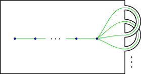
(a) The model for orientable surface braid groups.

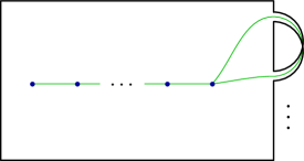
(b) The model for non-orientable surface braid groups.

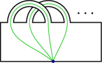
(c) The model for orientable mapping class groups.

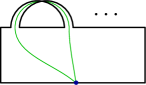
(d) The model for non-orientable mapping class groups.

Figure 2.1: Four examples of the setting of Lemma 2.1 where $S$ is a compact, connected surface with one boundary component, $\Gamma$ is the embedded graph (in green) and $A$ is its set of vertices (blue).

The key setting for the rest of the paper will be the second point of Examples 2.3, which we now consider in more detail. Let $S$ be a connected, compact surface with one boundary component, let $\Gamma$ be the embedded graph pictured in Figure 2.1 and let $A$ denote the set of vertices of $\Gamma$.

To apply Lemma 2.1, it will be convenient to modify these spaces a little in cases (a) and (b) of Figure 2.1, where the vertices lie in the interior of $S$. In these cases, let $\overline{S}$ be the result of blowing up each vertex of $\Gamma$ to a boundary component (so that the total number of boundary components of $\overline{S}$ is $\lvert A\rvert+1$), let $\overline{\Gamma}$ be the result of replacing each vertex $v$ of $\Gamma$ with a circle (coinciding with the corresponding new boundary component of $\overline{S}$) subdivided into $\nu(v)$ vertices and $\nu(v)$ edges, where $\nu(v)$ is the valence of $v$, and finally let $\overline{A}\subset\overline{\Gamma}$ be the union of these circles (equivalently, the new boundary components of $\overline{S}$). We clearly have homeomorphisms $\overline{S}\smallsetminus\overline{A}\cong S\smallsetminus A$ and $\overline{\Gamma}\smallsetminus\overline{A}\cong\Gamma\smallsetminus A$. In cases (c) and (d) of Figure 2.1, we simply take $\overline{S}=S$, $\overline{\Gamma}=\Gamma$ and $\overline{A}=A$.

By Lemma 2.1, the inclusion

$$C_{\mathbf{k}}(\Gamma\smallsetminus A)\cong C_{\mathbf{k}}(\overline{\Gamma}\smallsetminus\overline{A})\lhook\joinrel\longrightarrow C_{\mathbf{k}}(\overline{S}\smallsetminus\overline{A})\cong C_{\mathbf{k}}(S\smallsetminus A)$$ (2.4)

induces isomorphisms on Borel-Moore homology for all local coefficient systems on $C_{\mathbf{k}}(\overline{S}\smallsetminus\overline{A})$ that extend to $C_{\mathbf{k}}(\overline{S})$. But $\overline{A}$ is contained in the boundary of $\overline{S}$ (the purpose of replacing $S,\Gamma,A$ with $\overline{S},\overline{\Gamma},\overline{A}$ was precisely to ensure this) so, by Remark 2.2, the inclusion (2.4) induces isomorphisms on Borel-Moore homology with all local coefficient systems.

The twisted Borel-Moore homology of $C_{\mathbf{k}}(S\smallsetminus A)$ may therefore be computed from the twisted Borel-Moore homology of $C_{\mathbf{k}}(\Gamma\smallsetminus A)$, where we may now consider $\Gamma$ as an abstract graph (forgetting its embedding into $S$) with vertex set $A$, as depicted in Figure 2.2. Since the complement $\Gamma\smallsetminus A$ is simply the disjoint union of the (open) edges of the graph $\Gamma$, its configuration space $C_{\mathbf{k}}(\Gamma\smallsetminus A)$ is a disjoint union of open $k$-dimensional simplices, one for each choice of:

• the number of points that lie on each edge of $\Gamma$;

• for each edge of $\Gamma$, an ordered list of blocks of the partition $\mathbf{k}$, prescribing which blocks of the partition the configuration points that lie on this edge must belong to, as we pass from left to right along the edge (with respect to an arbitrary orientation of the edge, chosen once and for all).

This combinatorial information may be summarised succinctly as a choice, for each edge $e$ of $\Gamma$, of a word $w_{e}$ on the alphabet of blocks of the partition $\mathbf{k}$. This choice must have the property that the total number of times that a block of $\mathbf{k}$ appears in $w_{e}$, as $e$ runs over all edges of $\Gamma$, is equal to the size of the block. In this notation, the labelled graphs depicted in Figure 2.2 correspond to the different components of the configuration space $C_{\mathbf{k}}(\Gamma\smallsetminus A)$ as the set of labels $\{w_{e}\}_{e}$ varies.

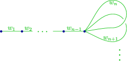
(a) The graph for orientable surface braid groups.

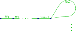
(b) The graph for non-orientable surface braid groups.

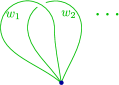
(c) The graph for orientable mapping class groups.

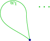
(d) The graph for non-orientable mapping class groups.

Figure 2.2: The graphs from Figure 2.1, considered now as abstract graphs and equipped with labels, viewed as generators of the Borel-Moore homology of $C_{\mathbf{k}}(\Gamma\smallsetminus A)$; equivalently, by Proposition 2.4, the Borel-Moore homology of $C_{\mathbf{k}}(S\smallsetminus A)$.

We summarise this discussion in the following result.

Proposition 2.4

Let $S$ be a connected, compact surface with one boundary component, let $A$ be either a finite subset of its interior or a single point on its boundary and let $\mathbf{k}$ be a partition of a positive integer $k$. Then there is a map

$$\bigsqcup_{w}\mathring{\Delta}^{k}\longrightarrow C_{\mathbf{k}}(S\smallsetminus A),$$ (2.5)

where $\mathring{\Delta}^{k}$ denotes the open $k$-dimensional simplex, that induces isomorphisms on Borel-Moore homology in all degrees and with coefficients in any local system $\mathcal{L}$ on $C_{\mathbf{k}}(S\smallsetminus A)$ defined over a ring $R$. The disjoint union on the left-hand side of (2.5) is indexed by functions

$$w\colon\{\text{edges of }\Gamma\}\longrightarrow\{\text{blocks of }\mathbf{k}\}^{*},$$ (2.6)

where $\Gamma$ is the abstract graph depicted in Figure 2.2, the notation $X^{*}$ means the monoid of words on a set $X$ and the total number of times that a block of $\mathbf{k}$ appears in the word $w_{e}$, as $e$ runs over all edges of $\Gamma$, is equal to the size of the block. Thus the Borel-Moore homology $H_{*}^{\mathrm{BM}}(C_{\mathbf{k}}(S\smallsetminus A);\mathcal{L})$ is concentrated in degree $k$ and the $R$-module

$$H_{k}^{\mathrm{BM}}(C_{\mathbf{k}}(S\smallsetminus A);\mathcal{L})$$ (2.7)

decomposes as a direct sum of copies of the fibre of $\mathcal{L}$, indexed by the combinatorial data (2.6).

Notation 2.5

It will be convenient later to fix some standard notation for the different parts of the graphs $\Gamma$ appearing in Proposition 2.4 and depicted in Figure 2.2. In cases (a) and (b), assuming that there are $n$ punctures, i.e. $\lvert A\rvert=n$, let us write $\mathbb{I}_{n}$ for the linear (or “tail”) part of the graph, which is a linear graph with $n$ vertices and $n-1$ edges. When the surface $S$ is orientable (cases (a) and (c)), we write $\mathbb{W}_{g}^{\Sigma}$ for the “wedge” part of the graph, which is a graph with one vertex and $2g$ edges, where $g$ is the genus of $S$. When the surface $S$ is non-orientable (cases (b) and (d)), we write instead $\mathbb{W}_{h}^{\mathscr{N}}$ for the “wedge” part of the graph, which is a graph with one vertex and $h$ edges, where $h$ is the non-orientable genus of $S$. The elements (2.6) of the set indexing the decomposition of (2.7) will typically be denoted by

$$(w_{1},\ldots,w_{n-1},[w_{n},w_{n+1}],\ldots,[w_{n+2g-2},w_{n+2g-1}])$$ (2.8)

when $S=\Sigma_{g,1}$ and by

$$(w_{1},\ldots,w_{n-1},[w_{n}],\ldots,[w_{n+h-1}])$$ (2.9)

when $S=\mathscr{N}_{h,1}$. The first $n-1$ terms are the values of $w$ on $\mathbb{I}_{n}$ and the remaining $2g$ respectively $h$ terms in square brackets are the values of $w$ on $\mathbb{W}_{g}^{\Sigma}$ respectively $\mathbb{W}_{h}^{\mathscr{N}}$.

Recall from Definition 1.10 the notion of the dual surface of a punctured surface, which we will apply to the surfaces depicted in Figure 2.1. In cases (a) and (b), the blow-up $\overline{S}$ is obtained from the punctured surface $S\smallsetminus A$ by blowing up each (interior) puncture in $A$ to a new boundary component and the dual surface $\check{S}$ is given by removing the original boundary component $\partial S$ from $\overline{S}$ but keeping the $\lvert A\rvert$ new boundary components. In cases (c) and (d), the blow-up $\overline{S}$ simply replaces the single boundary puncture $A$ in $\partial S$ with a closed interval and the dual surface $\check{S}$ is the union of the interior of $S$ with this closed interval in the boundary of $\overline{S}$.

The twisted Borel-Moore homology $H_{*}^{\mathrm{BM}}(C_{\mathbf{k}}(\check{S});\mathcal{L})$ has an explicit description similar to that of $H_{*}^{\mathrm{BM}}(C_{\mathbf{k}}(S\smallsetminus A);\mathcal{L})$ in Proposition 2.4. This is another direct application of Lemma 2.1, this time applied to the triple $(M^{\prime},B^{\prime},A^{\prime})$ where $M^{\prime}=\overline{S}$, $A^{\prime}=\partial(S\smallsetminus A)$ (so that $M^{\prime}\smallsetminus A^{\prime}=\check{S}$) and $B^{\prime}$ equal to the union of $A^{\prime}$ with the green arcs pictured in Figure 2.3. We record this here:

Proposition 2.6

Let $S$ and $A$ be as in Proposition 2.4 and define $\check{S}$ as in Definition 1.10. Let $\mathbf{k}$ be a partition of a positive integer $k$. Then the statement of Proposition 2.4 holds with $S\smallsetminus A$ replaced with $\check{S}$ and using the graphs of Figure 2.3 instead of those of Figure 2.2.

More precisely, the graphs of Figure 2.3 should be interpreted as follows in Proposition 2.6. Consider each collection of parallel arcs labelled by $w_{i}$ to be a single arc (the collections of parallel arcs will become relevant only in §2.3, for Definition 2.7). The set of labels $w_{1},w_{2},\ldots$ then describes the subspace of the configuration space where every configuration point lies in the interior of an arc and the sub-configuration lying on the $i$th arc consists of $\lvert w_{i}\rvert$ points belonging to the blocks of the partition $\mathbf{k}$ given by the letters of $w_{i}$ (with respect to an arbitrary orientation of the edge, chosen once and for all).

2.3 Dual bases

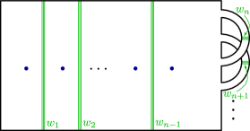
(a) Dual basis for orientable surface braid groups.

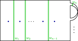
(b) Dual basis for non-orientable surface braid groups.

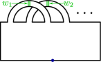
(c) Dual basis for orientable mapping class groups.

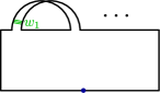
(d) Dual basis for non-orientable mapping class groups.

Figure 2.3: A linearly independent set of elements of $H_{k}(C_{\mathbf{k}}(S\smallsetminus A),\partial;\mathcal{L})$ whose span is isomorphic to the dual of $H_{k}^{\mathrm{BM}}(C_{\mathbf{k}}(S\smallsetminus A);\mathcal{L})$ via the perfect pairing (2.11). See Definition 2.7.

We now describe, using Poincaré-Lefschetz duality, a perfect pairing between (2.7) and another naturally-defined homology $R$-module, for which we describe a “dual” basis. In order to apply Poincaré-Lefschetz duality, we assume until the statement of Corollary 2.9 that the surface $S$ is orientable. By tensoring appropriately with the orientation local system, one may generalise this discussion to allow also non-orientable surfaces; this is explained in Corollary 2.9.

Let us now consider the relative homology group $H_{k}(C_{\mathbf{k}}(S\smallsetminus A),\partial;\mathcal{L})$, where $\partial$ is an abbreviation of $\partial C_{\mathbf{k}}(S\smallsetminus A)$, the boundary of the topological manifold $C_{\mathbf{k}}(S\smallsetminus A)$, which consists of all configurations that non-trivially intersect the boundary of $S\smallsetminus A$. In case (c), we implicitly make a small modification here: we replace $A$, which is a single point in $\partial S$, with a small closed interval in $\partial S$ and we correspondingly replace $S\smallsetminus A$ with the closure in $S$ of the complement of this small closed interval. In other words, similarly to the modification that we made in cases (a) and (b) in §2.2, we are blowing up the (unique) vertex of the graph $\Gamma$ on $\partial S$.

For this subsection, we assume that $\mathcal{L}$ is a rank-one local system; i.e. its fibre over each point is a free module of rank one over the ground ring $R$. In this case, the direct sum decomposition of Proposition 2.4 corresponds to a free basis for $H_{k}^{\mathrm{BM}}(C_{\mathbf{k}}(S\smallsetminus A);\mathcal{L})$ over $R$. There is a naturally corresponding set of elements of the relative homology group $H_{k}(C_{\mathbf{k}}(S\smallsetminus A),\partial;\mathcal{L})$, depicted in Figure 2.3 and indexed by the same combinatorial data as described in Proposition 2.4:

Definition 2.7

Consider one of the labelled graphs of Figure 2.3. Each of these is simply a disjoint union of collections of parallel arcs beginning and ending on the boundary of the surface, each labelled by a word $w_{i}$ on the alphabet of blocks of the partition $\mathbf{k}$. The number of parallel arcs in the collection labelled by $w_{i}$ is the length $\lvert w_{i}\rvert$ of this word, and each individual arc inherits a label which is the corresponding letter (i.e. block of $\mathbf{k}$) of this word (the parallel arcs in each collection are ordered using the orientation of the surface). The relative homology class depicted by this figure is the one represented by the relative cycle given by the subspace of configurations where exactly one point lies on each arc and this point belongs to the block of $\mathbf{k}$ specified by the label of the arc.

The relative homology classes described in Definition 2.7 are indexed by the same combinatorial data (2.6) as in Proposition 2.4, once we identify the edges of $\Gamma$ with the edges of its dual graph depicted in Figure 2.3 in the evident way (each edge of $\Gamma$ intersects precisely one edge of its dual graph).

As explained in [AP20, Th. A], the relative cap product and Poincaré-Lefschetz duality induce a pairing

$$H_{k}^{\mathrm{BM}}(C_{\mathbf{k}}(S\smallsetminus A);\mathcal{L})\otimes_{R}H_{k}(C_{\mathbf{k}}(S\smallsetminus A),\partial;\mathcal{L})\longrightarrow R$$ (2.10)

whose evaluation on a basis element of $H_{k}^{\mathrm{BM}}(C_{\mathbf{k}}(S\smallsetminus A);\mathcal{L})$ (from Proposition 2.4) together with an element of Definition 2.7 is equal to $1$ if the two elements are indexed by the same function $w$ and equal to $0$ otherwise. It follows that the submodule spanned by the elements of Definition 2.7 is freely spanned by them (i.e. they are linearly independent), and the pairing (2.10) restricts to a perfect pairing when we restrict to this submodule on the right-hand factor of its domain.

Notation 2.8

We write $H_{k}^{\partial}(C_{\mathbf{k}}(S\smallsetminus A);\mathcal{L})$ for the $R$-submodule of $H_{k}(C_{\mathbf{k}}(S\smallsetminus A),\partial;\mathcal{L})$ (freely) spanned by the elements defined in Definition 2.7. In general, for a module $W$ over a ring $R$, we denote by $W^{\vee}$ its linear dual $R$-module $\mathrm{Hom}_{R}(W,R)$.

With this notation, the discussion above may be summarised as follows.

Corollary 2.9

Let $S$ be a connected, compact, orientable surface with one boundary component, let $A$ be either a finite subset of its interior or a closed interval in its boundary and let $\mathbf{k}$ be a partition of a positive integer $k$. Choose any rank-one local system $\mathcal{L}$ on $C_{\mathbf{k}}(S\smallsetminus A)$ defined over a ring $R$. Then the $R$-module $H_{k}^{\partial}(C_{\mathbf{k}}(S\smallsetminus A);\mathcal{L})$ is freely generated over $R$ by the elements of Definition 2.7, indexed by the same combinatorial data as in Proposition 2.4. Moreover, there is a perfect pairing

$$H_{k}^{\mathrm{BM}}(C_{\mathbf{k}}(S\smallsetminus A);\mathcal{L})\otimes_{R}H_{k}^{\partial}(C_{\mathbf{k}}(S\smallsetminus A);\mathcal{L})\longrightarrow R,$$ (2.11)

given by the relative cap product and Poincaré-Lefschetz duality, whose matrix with respect to the two bases that we have described is the identity matrix. In particular, we therefore have

$$H_{k}^{\partial}(C_{\mathbf{k}}(S\smallsetminus A);\mathcal{L})\;\cong\;\left(H_{k}^{\mathrm{BM}}(C_{\mathbf{k}}(S\smallsetminus A);\mathcal{L})\right)^{\vee}.$$ (2.12)

When $S$ is non-orientable, there is also a perfect pairing (2.11), and thus an identification (2.12), with the only difference being that we must replace the local system $\mathcal{L}$ in the coefficients of $H_{k}^{\partial}(-)$ by $\mathcal{L}\otimes\mathcal{O}$, where $\mathcal{O}$ denotes the orientation local system of the non-orientable manifold $C_{\mathbf{k}}(S\smallsetminus A)$.

Remark 2.10

The perfect pairing (2.11) and the dual basis described in Definition 2.7 (and illustrated in Figure 2.3) will be used in some diagrammatic proofs in the next section, including in the proof of the “Cloud lemma” (Lemma 3.11).

Remark 2.11

Although we shall not need it in the present paper, we point out that there is an embedding (of mapping class group representations) from $H_{k}^{\partial}(C_{\mathbf{k}}(S\smallsetminus A);\mathcal{L})$ into $H_{k}^{\mathrm{BM}}(C_{\mathbf{k}}(\check{S});\mathcal{L})$, which acts diagonally with respect to the free bases described in Definition 2.7 and Proposition 2.6 respectively; see [AP20, Theorem B and Corollary C]. In light of the identification (2.12), when $\lvert A\rvert=n$ and $\mathcal{L}=\mathbb{Z}[Q_{(\mathbf{k},\ell)}]$ this is an embedding $\mathfrak{L}_{(\mathbf{k},\ell)}(\mathtt{n})^{\vee}\hookrightarrow\mathfrak{L}^{v}_{(\mathbf{k},\ell)}(\mathtt{n})$.

3 Short exact sequences

In this section, we construct the fundamental short exact sequences for homological representation functors of Theorem B. We start by recalling the categorical background of these short exact sequences in §3.1. Then we construct the short exact sequences for the functors of surface braid groups in §3.2, and in §3.3 for those of mapping class groups of surfaces. Throughout §3, we consider homological representation functors indexed by a partition $\mathbf{k}=\boldsymbol{\{}k_{1};\ldots;k_{r}\boldsymbol{\}}\vdash k$ of an integer $k\geqslant 1$ and by the stage $\ell\geqslant 1$ of a lower central series.

3.1 Background and preliminaries

This section recollects the key categorical tools that define the setting in which we unearth the short exact sequences of homological representation functors of §3.2 and §3.3. We also prepare the work of these sections with an important foreword in §3.1.2.

3.1.1 Short exact sequences induced from the categorical framework

We recollect here the notions and first properties of translation, difference and evanescence functors, which give rise to the key natural short exact sequences that we study for homological representation functors in §3.2 and §3.3. The following definitions and results extend verbatim to the present slightly larger framework from the previous literature on this topic; see [DV19] and [Sou22, §4] for instance. The various proofs are straightforward generalisations of these previous works. For the remainder of §3.1, we fix an abelian category $\mathcal{A}$, a strict left-module $(\mathcal{M},\natural)$ over a strict monoidal small groupoid $(\mathcal{G},\natural,\mathtt{0})$, where $\mathcal{M}$ is a small (skeletal) groupoid, $(\mathcal{G},\natural,\mathtt{0})$ has no zero divisors and $\mathrm{Aut}_{\mathcal{G}}(\mathtt{0})=\{\mathrm{id}_{\mathtt{0}}\}$. We assume that $\mathcal{M}$ and $\mathcal{G}$ have the same set of objects, identified with the non-negative integers $\mathbb{N}$, with the standard notation $\mathtt{n}$ to denote an object, and that both the monoidal and module structures $\natural$ are given on objects by addition. In particular, this is consistent with the fact that $\mathtt{0}$ is the unit for the monoidal structure of $\mathcal{G}$. One quickly checks that all the groupoids of the types of $\mathcal{M}$ and $\mathcal{G}$ defined in §1.3 satisfy all of these assumptions.

For an object $\mathtt{n}$ of $\mathcal{G}$, let $\tau_{\mathtt{n}}$ be the endofunctor of the functor category $\mathbf{Fct}(\langle\mathcal{G},\mathcal{M}\rangle,\mathcal{A})$ defined by $\tau_{\mathtt{n}}(F)=F(\mathtt{n}\natural-)$, called the translation functor. Let $i_{\mathtt{n}}\colon\mathit{Id}\to\tau_{\mathtt{n}}$ be the natural transformation of $\mathbf{Fct}(\mathcal{M},\mathcal{A})$ defined by precomposition with the morphisms $[\mathtt{n},\mathrm{id}_{\mathtt{n}\natural\mathtt{m}}]\colon\mathtt{m}\to\mathtt{n}\natural\mathtt{m}$ for each $\mathtt{m}\in\mathrm{Obj}(\mathcal{M})$. We define $\delta_{\mathtt{n}}=\mathrm{coker}(i_{\mathtt{n}})$, called the difference functor, and $\kappa_{\mathtt{n}}=\mathrm{ker}(i_{\mathtt{n}})$, called the evanescence functor. We denote by $\tau_{\mathtt{n}}^{d}$ and $\delta_{\mathtt{n}}^{d}$ the $d$-fold iterations $\tau_{\mathtt{n}}\cdots\tau_{\mathtt{n}}\tau_{\mathtt{n}}$ and $\delta_{\mathtt{n}}\cdots\delta_{\mathtt{n}}\delta_{\mathtt{n}}$ respectively. The translation functor $\tau_{\mathtt{n}}^{d}$ is by definition naturally isomorphic to $\tau_{\mathtt{n}^{d}}$.

The translation functor $\tau_{\mathtt{n}}$ is exact and induces the following exact sequence of endofunctors of $\mathbf{Fct}(\langle\mathcal{G},\mathcal{M}\rangle,\mathcal{A})$:

$$0\longrightarrow\kappa_{\mathtt{n}}\overset{\Omega_{\mathtt{n}}}{\longrightarrow}\mathit{Id}\overset{i_{\mathtt{n}}}{\longrightarrow}\tau_{\mathtt{n}}\overset{\Delta_{\mathtt{n}}}{\longrightarrow}\delta_{\mathtt{n}}\longrightarrow 0.$$ (3.1)

Moreover, for a short exact sequence $0\longrightarrow F\longrightarrow G\longrightarrow H\longrightarrow 0$ in the category $\mathbf{Fct}(\langle\mathcal{G},\mathcal{M}\rangle,\mathcal{A})$, there is a natural exact sequence defined from the snake lemma:

$$0\longrightarrow\kappa_{\mathtt{n}}F\longrightarrow\kappa_{\mathtt{n}}G\longrightarrow\kappa_{\mathtt{n}}H\longrightarrow\delta_{\mathtt{n}}F\longrightarrow\delta_{\mathtt{n}}G\longrightarrow\delta_{\mathtt{n}}H\longrightarrow 0.$$ (3.2)

In addition, for $\mathtt{n},\mathtt{m}\in\mathrm{Obj}(\mathcal{G})$, $\tau_{\mathtt{n}}$ and $\tau_{\mathtt{m}}$ commute up to natural isomorphism and they commute with limits and colimits; $\delta_{\mathtt{n}}$ and $\delta_{\mathtt{m}}$ commute up to natural isomorphism and they commute with colimits; $\kappa_{\mathtt{n}}$ and $\kappa_{\mathtt{m}}$ commute up to natural isomorphism and they commute with limits; and $\tau_{\mathtt{n}}$ commute with the functors $\delta_{\mathtt{m}}$ and $\kappa_{\mathtt{m}}$ up to natural isomorphism. Finally, for $F$ an object of $\mathbf{Fct}(\langle\mathcal{G},\mathcal{M}\rangle,\mathcal{A})$, we obtain the following natural exact sequence by applying the snake lemma twice:

$$0\longrightarrow\kappa_{\mathtt{n}}F\longrightarrow\kappa_{\mathtt{m}\natural\mathtt{n}}F\longrightarrow\kappa_{\mathtt{m}}\tau_{\mathtt{n}}F\longrightarrow\delta_{\mathtt{n}}F\longrightarrow\delta_{\mathtt{m}\natural\mathtt{n}}F\longrightarrow\delta_{\mathtt{m}}\tau_{\mathtt{n}}F\longrightarrow 0.$$ (3.3)

3.1.2 Preliminaries for the homological representation functors

We now briefly discuss some key preliminaries for the work of §3.2–§3.3. Throughout §3.1.2, we consider any one of the homological representation functors of §1.3. Following Notation 1.6, we denote it by $\mathfrak{L}^{\star}_{(\mathbf{k},\ell)}$ with $\mathbb{Z}[Q^{\star}_{(\mathbf{k},\ell)}]$ the ground ring of the target module category, where $\star$ either stands for the blank space or $\star=u$. We begin with the following general observations.

Observation 3.1

The short exact sequences that we exhibit in §3.2–§3.3 are applications of the exact sequence (3.1), with $\mathtt{n}=\mathtt{1}$, to each homological representation functor of §1.3. With a little more work, one could deduce analogous (though slightly more complex) results from (3.1) for any object $\mathtt{n}$. However, only the case $\mathtt{n}=\mathtt{1}$ will be needed in §4 to prove our polynomiality results, so we shall not pursue this generalisation here.

Subpartitions.

Our descriptions of the difference functor $\delta_{\mathtt{1}}\mathfrak{L}^{\star}_{(\mathbf{k},\ell)}$ in §3.2–§3.3 make key use of some appropriate partitions of $k-1$ obtained from $\mathbf{k}\vdash k$. We denote these partitions and their sets as follows:

Notation 3.2

For integers $k\geqslant k^{\prime}\geqslant 1$ and a partition $\mathbf{k}=\boldsymbol{\{}k_{1};\ldots;k_{r}\boldsymbol{\}}\vdash k$, we denote by $\{\mathbf{k}-k^{\prime}\}$ the set $\left\{\boldsymbol{\{}k_{1}-k^{\prime}_{1};\ldots;k_{r}-k^{\prime}_{r}\boldsymbol{\}}\bigm{|}0\leqslant k^{\prime}_{i}\leqslant k_{i}\textrm{ such that }\sum_{1\leqslant l\leqslant r}k^{\prime}_{l}=k^{\prime}\right\}$.

When $k^{\prime}=1$, we denote by $\mathbf{k}_{i}$ the element $\boldsymbol{\{}k_{1};\ldots;k_{i}-1;\ldots;k_{r}\boldsymbol{\}}$ of $\{\mathbf{k}-1\}$, for each $1\leqslant i\leqslant r$ such that $k_{i}\geqslant 1$.

When $k^{\prime}=2$, we denote by $\mathbf{k}_{i,j}$ the element $\boldsymbol{\{}k_{1};\ldots;k_{i}-1;\ldots;k_{j}-1;\ldots;k_{r}\boldsymbol{\}}$ of $\{\mathbf{k}-2\}$, for each $1\leqslant i<j\leqslant r$ such that $k_{i}\geqslant 1$ and $k_{j}\geqslant 1$. We similarly denote by $\mathbf{k}_{i,i}$ the element $\boldsymbol{\{}k_{1};\ldots;k_{i}-2;\ldots;k_{r}\boldsymbol{\}}$ of $\{\mathbf{k}-2\}$, for each $1\leqslant i\leqslant r$ such that $k_{i}\geqslant 2$.

Furthermore, we deal with partitions where some blocks may be null as follows. Let us consider $\mathbf{h}=\boldsymbol{\{}h_{1};\ldots;h_{r}\boldsymbol{\}}\vdash h$ with $h\geqslant 0$ such that $0\leqslant h_{l}\leqslant h$ for all $1\leqslant l\leqslant r$. We denote by $\overline{\mathbf{h}}$ the partition of $h$ obtained from $\mathbf{h}$ by removing the $0$-blocks. Then, we always identify $\mathfrak{L}^{\star}_{(\mathbf{h},\ell)}$ with $\mathfrak{L}^{\star}_{(\overline{\mathbf{h}},\ell)}$ since these functors are obviously isomorphic. Also, as a convention, we define the homological representation functors of §1.3.2 and §1.3.3 for $k=0$ as follows:

Notation 3.3

Except for the Lawrence-Bigelow functors (see Notation 3.13), we denote by $\mathfrak{L}^{\star}_{(0,\ell)}$ the functor $\langle\mathcal{G},\mathcal{M}\rangle\to{\mathbb{Z}[Q^{\star}_{((1),\ell)}]}{}\textrm{-}\mathrm{Mod}^{\mathrm{tw}}$ sending each object $\mathtt{n}$ to $\mathbb{Z}[Q^{\star}_{((1),\ell)}]$, the canonical action on $\mathbb{Z}[Q^{\star}_{((1),\ell)}]$ of the groups $G_{n}$ for the automorphisms and the identity for the morphisms of type $[\mathtt{m},\mathrm{id}_{\mathtt{m}\natural\mathtt{n}}]$ for $m>0$.

Twisted functors.

Let us now consider a homological representation functor $\mathfrak{L}^{\star}_{(\mathbf{k},\ell)}=\mathfrak{L}_{(\mathbf{k},\ell)}$ that is twisted, i.e. where $\mathfrak{L}_{(\mathbf{k},\ell)}\neq\mathfrak{L}^{u}_{(\mathbf{k},\ell)}$ has a category of twisted modules ${\mathbb{Z}[Q_{(\mathbf{k},\ell)}]}{}\textrm{-}\mathrm{Mod}^{\mathrm{tw}}$ as its target; see Definition 1.5. (Recall that we sometimes have $\mathfrak{L}_{(\mathbf{k},\ell)}=\mathfrak{L}^{u}_{(\mathbf{k},\ell)}$, e.g. if $\ell\leqslant 2$; see Lemma 1.9.) The problem arising in this setting is that the category ${\mathbb{Z}[Q_{(\mathbf{k},\ell)}]}{}\textrm{-}\mathrm{Mod}^{\mathrm{tw}}$ is not abelian (because it lacks a null object), while this is a necessary condition of the categorical framework to introduce the exact sequences of §3.1.1 and later to define polynomiality in §4.1. However, this subtlety does not impact the core ideas we deal with, and we solve this minor issue by adopting the following convention:

Convention 3.4

Throughout §3, when we consider a twisted homological representation functor $\mathfrak{L}_{(\mathbf{k},\ell)}$, we always postcompose it by the forgetful functor ${\mathbb{Z}[Q_{(\mathbf{k},\ell)}]}{}\textrm{-}\mathrm{Mod}^{\mathrm{tw}}\to{\mathbb{Z}}{}\textrm{-}\mathrm{Mod}$ as in (1.6). A fortiori, the target category of $\mathfrak{L}^{\star}_{(\mathbf{k},\ell)}$ is either ${\mathbb{Z}}{}\textrm{-}\mathrm{Mod}$ if $\mathfrak{L}^{\star}_{(\mathbf{k},\ell)}$ is twisted, and it is ${\mathbb{Z}[Q_{(\mathbf{k},\ell)}]}{}\textrm{-}\mathrm{Mod}$ otherwise. Following Notation 1.6, we denote by ${\mathbb{Z}[Q^{\star}_{(\mathbf{k},\ell)}]}{}\textrm{-}\mathrm{Mod}^{\bullet}$ the target category of $\mathfrak{L}^{\star}_{(\mathbf{k},\ell)}$ under this convention.

Change of rings operations.

Finally, we explain some key manipulations of the transformation groups associated to homological representation functors. Let $R$ be an associative unital ring. For a category $\mathcal{C}$ and a ring homomorphism $f\colon\mathbb{Z}[Q]\to R$, the change of rings operation on a functor $F\colon\mathcal{C}\to{\mathbb{Z}[Q]}{}\textrm{-}\mathrm{Mod}^{*}$ consists in composing with the induced module functor $f_{!}\colon{\mathbb{Z}[Q]}{}\textrm{-}\mathrm{Mod}^{*}\to R{}\textrm{-}\mathrm{Mod}^{*}$, also known as the tensor product functor $R\otimes_{f}-$, where $*$ either stands for the blank space or $*=\mathrm{tw}$. A key use of the change of rings operations is the following natural modification of the ground rings of homological representation functors with respect to partitions.

Using the notation of §1.2.1, we consider partitions $\mathbf{k}=\boldsymbol{\{}k_{1};\ldots;k_{r}\boldsymbol{\}}\vdash k$ and $\mathbf{k}^{\prime}=\boldsymbol{\{}k_{1}^{\prime};\ldots;k_{r}^{\prime}\boldsymbol{\}}\vdash k^{\prime}$ such that $1\leqslant k^{\prime}\leqslant k$, $k_{l}\geqslant 1$ and $0\leqslant k^{\prime}_{l}\leqslant k_{l}$ for all $1\leqslant l\leqslant r$. For each $k^{\prime}_{i}<k_{i}$, there is an evident analogue of the short exact sequence (1.4) with $G_{k^{\prime}_{i},n}$ as quotient and $G_{\boldsymbol{\{}k_{i}-k^{\prime}_{i},k^{\prime}_{i}\boldsymbol{\}},n}$ as the middle term. The section $s_{\boldsymbol{\{}k_{i}-k^{\prime}_{i},k^{\prime}_{i}\boldsymbol{\}},n}$ of that short exact sequence provides an injection $G_{k^{\prime}_{i},n}\hookrightarrow G_{\boldsymbol{\{}k_{i}-k^{\prime}_{i},k^{\prime}_{i}\boldsymbol{\}},n}$. Composing this with the canonical injection $G_{\boldsymbol{\{}k_{i}-k^{\prime}_{i},k^{\prime}_{i}\boldsymbol{\}},n}\hookrightarrow G_{k_{i},n}$, we obtain an injection $G_{k^{\prime}_{i},n}\hookrightarrow G_{k_{i},n}$. Applying this procedure for each block, we obtain a canonical injection $G_{\mathbf{k}^{\prime},n}\hookrightarrow G_{\mathbf{k},n}$. Now, for some fixed $\ell\geqslant 1$, we consider the transformation groups $Q^{\star}_{(\mathbf{k},\ell)}$ and $Q^{\star}_{(\mathbf{k}^{\prime},\ell)}$ associated to homological representation functors $\mathfrak{L}^{\star}_{(\mathbf{k},\ell)}$ and $\mathfrak{L}^{\star}_{(\mathbf{k}^{\prime},\ell)}$ respectively.

Lemma 3.5

There is a canonical group homomorphism $\mathcal{Q}_{(\mathbf{k}^{\prime}\to\mathbf{k},\ell)}\colon Q^{\star}_{(\mathbf{k}^{\prime},\ell)}\longrightarrow Q^{\star}_{(\mathbf{k},\ell)}$.

Proof.

The injection $G_{\mathbf{k}^{\prime},n}\hookrightarrow G_{\mathbf{k},n}$ induces the following commutative triangle:

Taking kernels and the colimit as $n\to\infty$, we uniquely define the morphism $\mathcal{Q}_{(\mathbf{k}^{\prime}\to\mathbf{k},\ell)}$. ∎

In §3.2–§3.3, we will apply a change of rings operation using morphisms of the type $\mathcal{Q}_{(\mathbf{k}^{\prime}\to\mathbf{k},\ell)}$ and use the following property:

Observation 3.6

The change of rings operation $(\mathbb{Z}[\mathcal{Q}_{(\mathbf{k}^{\prime}\to\mathbf{k},\ell)}])_{!}\colon\mathbb{Z}[Q^{\star}_{(\mathbf{k}^{\prime},\ell)}]{}\textrm{-}\mathrm{Mod}^{*}\to\mathbb{Z}[Q^{\star}_{(\mathbf{k},\ell)}]{}\textrm{-}\mathrm{Mod}^{*}$ gives $\mathfrak{L}^{\star}_{(\mathbf{k}^{\prime},\ell)}$ the same ground ring as $\mathfrak{L}^{\star}_{(\mathbf{k},\ell)}$. In the case when $*=\mathrm{tw}$, it also gives $\mathfrak{L}^{\star}_{(\mathbf{k}^{\prime},\ell)}$ the same action of each group $G_{n}$ on $\mathbb{Z}[Q^{\star}_{(\mathbf{k}^{\prime},\ell)}]$ as $\mathfrak{L}^{\star}_{(\mathbf{k},\ell)}$.

Hence, the change of rings operation $(\mathbb{Z}[\mathcal{Q}_{(\mathbf{k}^{\prime}\to\mathbf{k},\ell)}])_{!}$ allows us to canonically switch the module structure of $\mathfrak{L}^{\star}_{(\mathbf{k}^{\prime},\ell)}$ from $\mathbb{Z}[Q^{\star}_{(\mathbf{k}^{\prime},\ell)}]$ to $\mathbb{Z}[Q^{\star}_{(\mathbf{k},\ell)}]$, as well as the potential twisted structure, i.e. actions of the groups $G_{n}$ on these modules. In particular, we use this type of operation to identify $\mathfrak{L}^{\star}_{(\mathbf{k}^{\prime},\ell)}$ as a summand of the difference functor $\delta_{\mathtt{1}}\mathfrak{L}^{\star}_{(\mathbf{k},\ell)}$ in §3.2–§3.3. This change of ground ring map is just the identity in many situations, and in any case it does not impact the key underlying structures of $\mathfrak{L}^{\star}_{(\mathbf{k}^{\prime},\ell)}$ for our work. Because these subtleties are minor points and do not affect the key points of the reasoning, we choose to use the following conventions to simplify the notation:

Convention 3.7

Throughout §3.2–§3.3, change of ground ring operations $(\mathbb{Z}[\mathcal{Q}_{(\mathbf{k}^{\prime}\to\mathbf{k},\ell)}])_{!}$ must be applied in order to properly identify the functor $\mathfrak{L}^{\star}_{(\mathbf{k}^{\prime},\ell)}$ as a summand of $\delta_{1}\mathfrak{L}^{\star}_{(\mathbf{k},\ell)}$. However, we generally keep the notation $\mathfrak{L}^{\star}_{(\mathbf{k}^{\prime},\ell)}$ for this modified functor for the sake of simplicity and to avoid overloading the notation, insofar as all these change of rings operations are clear from the context.

Finally, the following lemma will be the key point justifying that a change of rings operation does not impact the results of §3.2–§3.3.

Lemma 3.8

Let $Q$ be a group, $R$ a ring and $f\colon\mathbb{Z}[Q]\to R$ a ring homomorphism. We consider a functor $F\colon\langle\mathcal{G},\mathcal{M}\rangle\to{\mathbb{Z}[Q]}{}\textrm{-}\mathrm{Mod}$ such that $\kappa_{\mathtt{1}}F=0$ and so that $F(\mathtt{n})$, $\tau_{\mathtt{1}}F(\mathtt{n})$ and $\delta_{\mathtt{1}}F(\mathtt{n})$ are free $\mathbb{Z}[Q]$-modules for all $\mathtt{n}\in\mathrm{Obj}(\mathcal{M})$. If $\delta_{\mathtt{1}}F=0$, then both $\delta_{\mathtt{1}}f_{!}F=0$ and $\kappa_{\mathtt{1}}f_{!}F=0$.

The same statement also holds if $F$ takes values in $\mathbb{Z}[Q]{}\textrm{-}\mathrm{Mod}^{\mathrm{tw}}$. In this case, the change of rings operation $f_{!}$ takes place at the level of twisted module categories $\mathbb{Z}[Q]{}\textrm{-}\mathrm{Mod}^{\mathrm{tw}}\to R{}\textrm{-}\mathrm{Mod}^{\mathrm{tw}}$ but, as explained in Convention 3.4, all of the statements take place in the category of functors into $\mathbb{Z}{}\textrm{-}\mathrm{Mod}$, via post-composing with the forgetful functor.

Proof.

We first note that the functor $f_{!}$ commutes with the translation functor $\tau_{\mathtt{1}}$. The result then follows from the fact that the functor $f_{!}$ turns split short exact sequences of $\mathbb{Z}[Q]$-modules to split short exact sequences of $R$-modules. ∎

3.2 For surface braid group functors

We prove in §3.2.2 and §3.2.3 our results on short exact sequences of Theorem B for surface braid group functors. The proofs of these results require certain diagrammatic arguments, which we explain first in §3.2.1. For the remainder of §3.2, we consider any one of the homological representation functors of (1.11) and (1.12) with the classical (i.e. non-vertical) setting. Following Notation 1.6, we generically denote it by $\mathfrak{L}^{\star}_{(\mathbf{k},\ell)}(S)$ where $\star$ either stands for the blank space or $\star=u$, $S\in\{\mathbb{D},\Sigma_{g,1},\mathscr{N}_{h,1}\}$ with $g\geqslant 1$ and $h\geqslant 1$, and the associated transformation group is denoted by $Q^{\star}_{(\mathbf{k},\ell)}(S)$. This generic notation is the same as that of (1.12), and in particular this is the Lawrence-Bigelow functor $\mathfrak{LB}^{\star}_{(\mathbf{k},\ell)}$ in the case when $S=\mathbb{D}$.

3.2.1 Preliminary properties and diagrammatic arguments

We start here with some first observations and qualitative properties of the representations to prepare the work of §3.2.2 and §3.2.3. First and foremost, we recall that we have introduced model graphs $\mathbb{I}_{n}$, $\mathbb{W}_{g}^{\Sigma}$ and $\mathbb{W}_{h}^{\mathscr{N}}$ in Notation 2.5, modelled by Figures 1(a) and 1(b). Let us abbreviate by writing $\mathbb{W}^{S}=\mathbb{W}_{g}^{\Sigma}$ if $S=\Sigma_{g,1}$ and $\mathbb{W}^{S}=\mathbb{W}_{h}^{\mathscr{N}}$ if $S=\mathscr{N}_{h,1}$.

Remark 3.9

For convenience, the diagrammatic arguments below illustrated in Figures 3.1–3.3 are drawn only with the case $S=\Sigma_{g,1}$. Indeed, only the planar parts of these figures are important: to obtain the case $S=\mathscr{N}_{h,1}$, one simply has to modify the right-hand sides of Figures 3.1–3.3 with non-orientable handles of the type of Figure 1(b), while we simply cut this right-hand side off to obtain the case $S=\mathbb{D}$.

We take up the notations of §2.2 and we consider, for each $\mathtt{n}\in\mathrm{Obj}(\boldsymbol{\beta}^{S})$, the surface braid group $\mathbf{B}_{n}(S)$ representation $\mathfrak{L}^{\star}_{(\mathbf{k},\ell)}(S)(\mathtt{n})=H_{k}^{\mathrm{BM}}(C_{\mathbf{k}}(\mathbb{D}_{n}\natural S);\mathbb{Z}[Q^{\star}_{(\mathbf{k},\ell)}(S)])$ where $\mathbb{Z}[Q^{\star}_{(\mathbf{k},\ell)}(S)]$ is a rank-one local system explained in the general construction of §1.2. Proposition 2.4 describes a free basis for the underlying $\mathbb{Z}[Q^{\star}_{(\mathbf{k},\ell)}(S)]$-module of $\mathfrak{L}^{\star}_{(\mathbf{k},\ell)}(S)(\mathtt{n})$ indexed by labellings of the embedded graph $\mathbb{I}_{n}\vee\mathbb{W}^{S}\subset S$ by words in the blocks of the partition $\mathbf{k}$. More precisely, the basis is the set of tuples of the form (2.8) if $S=\Sigma_{g,1}$ and (2.9) if $S=\mathscr{N}_{h,1}$. We use the following slight simplification of Notation 2.5 for §3.2.

Notation 3.10

Let $g_{S}$ denote the genus of the surface $S$ (i.e. $2g$ if $S=\Sigma_{g,1}$ and $h$ if $S=\mathscr{N}_{h,1}$). For the sake of simplicity, we generically write the basis elements (2.8) and (2.9) as $(w_{1},\ldots,w_{g_{S}+n-1})$ since the diagrammatic arguments of this subsection work in the same way for both the orientable surfaces and non-orientable ones. Also, choosing an ordering of the edges of the embedded graph $\mathbb{I}_{n}\vee\mathbb{W}^{S}\subset\mathbb{D}_{n}\natural S$, we write $(w_{1},\ldots,w_{g_{S}+n-1})\vdash\mathbf{k}$ in order to indicate that the basis element $(w_{1},\ldots,w_{g_{S}+n-1})$ is a tuple of words in the alphabet $\{1,2,\ldots,r\}$ such that each letter $i\in\{1,2,\ldots,r\}$ appears precisely $k_{i}$ times.

The representation $\tau_{\mathtt{1}}\mathfrak{L}^{\star}_{(\mathbf{k},\ell)}(S)(\mathtt{n})=H_{k}^{\mathrm{BM}}(C_{\mathbf{k}}(\mathbb{D}_{1+n}\natural S);\mathbb{Z}[Q^{\star}_{(\mathbf{k},\ell)}(S)])$ has a very similar description as a free module: the only difference is that there is one extra edge of the embedded graph $\mathbb{I}_{1+n}\vee\mathbb{W}^{S}\subset\mathbb{D}_{1+n}\natural S$ whose edge-labellings index the free generating set for $\tau_{\mathtt{1}}\mathfrak{L}^{\star}_{(\mathbf{k},\ell)}(S)(\mathtt{n})$. We write this as $(w_{0},w_{1},\ldots,w_{g_{S}+n-1})\vdash\mathbf{k}$, where $w_{0}$ is the label of the extra edge. Now, we recall from Lemma 1.7 that the image of the canonical morphism $[\mathtt{1},\mathrm{id}_{\mathtt{1}\natural\mathtt{n}}]\in\langle\boldsymbol{\beta},\boldsymbol{\beta}^{S}\rangle(\mathtt{n},\mathtt{1}\natural\mathtt{n})$ by $\mathfrak{L}^{\star}_{(\mathbf{k},\ell)}(S)$ is the map $H_{k}^{\mathrm{BM}}(C_{\mathbf{k}}(\mathbb{D}_{n}\natural S);\mathbb{Z}[Q^{\star}_{(\mathbf{k},\ell)}(S)])\to H_{k}^{\mathrm{BM}}(C_{\mathbf{k}}(\mathbb{D}_{1+n}\natural S);\mathbb{Z}[Q^{\star}_{(\mathbf{k},\ell)}(S)])$ induced by the evident inclusion of configuration spaces $C_{\mathbf{k}}(\mathbb{D}_{n}\natural S)\hookrightarrow C_{\mathbf{k}}(\mathbb{D}_{1}\natural(\mathbb{D}_{n}\natural S))$ coming from the boundary connected sum with the left-most copy of $\mathbb{D}_{1}$. In terms of the above free generating sets coming from Proposition 2.4, the map $\mathfrak{L}^{\star}_{(\mathbf{k},\ell)}(S)([\mathtt{1},\mathrm{id}_{\mathtt{1}\natural\mathtt{n}}])$ is thus the injection $(w_{1},\ldots,w_{g_{S}+n-1})\mapsto(\varnothing,w_{1},\ldots,w_{g_{S}+n-1})$. The cokernel $\delta_{\mathtt{1}}\mathfrak{L}^{\star}_{(\mathbf{k},\ell)}(S)(\mathtt{n})$ may therefore be described as the free $\mathbb{Z}[Q^{\star}_{(\mathbf{k},\ell)}(\mathbb{D})]$-module generated by all edge-labellings $(w_{0},w_{1},\ldots,w_{g_{S}+n-1})\vdash\mathbf{k}$ of $\mathbb{I}_{1+n}\vee\mathbb{W}^{S}$ such that $w_{0}$ is not the empty word, while $\kappa_{\mathtt{1}}\mathfrak{L}^{\star}_{(\mathbf{k},\ell)}(S)(\mathtt{n})=0$.

Furthermore, using Notation 3.2, the direct sum $\bigoplus_{i=1}^{r}\tau_{\mathtt{1}}\mathfrak{L}^{\star}_{(\mathbf{k}_{i},\ell)}(S)(\mathtt{n})$ then has a basis indexed by pairs $(i,(w_{0},w_{1},\ldots,w_{g_{S}+n-1}))$, where $1\leqslant i\leqslant r$ and $(w_{0},w_{1},\ldots,w_{g_{S}+n-1})\vdash\mathbf{k}_{i}$. There is an evident bijection between the basis for $\delta_{\mathtt{1}}\mathfrak{L}^{\star}_{(\mathbf{k},\ell)}(S)(\mathtt{n})$ and this basis for $\bigoplus_{i=1}^{r}\tau_{\mathtt{1}}\mathfrak{L}^{\star}_{(\mathbf{k}_{i},\ell)}(S)(\mathtt{n})$ given by

$$(w_{0},w_{1},\ldots,w_{g_{S}+n-1})\longmapsto(i,(w^{\prime}_{0},w_{1},\ldots,w_{g_{S}+n-1})),$$ (3.4)

where $w_{0}=iw^{\prime}_{0}$. Extending by linearity, this bijection determines an isomorphism of free modules

$$\delta_{\mathtt{1}}\mathfrak{L}^{\star}_{(\mathbf{k},\ell)}(S)(\mathtt{n})\overset{\cong}{\longrightarrow}\bigoplus_{i=1}^{r}\tau_{\mathtt{1}}\mathfrak{L}^{\star}_{(\mathbf{k}_{i},\ell)}(S)(\mathtt{n}).$$ (3.5)

The cloud lemma.

In order to construct the fundamental short exact sequences of Theorem B for surface braid groups, we will need to show that the isomorphism of modules (3.5) is in fact an isomorphism of representations. (In fact, we will show that it is moreover an isomorphism of functors as $n$ varies.) We assume that $\mathtt{n}\geqslant\mathtt{2}$. The key ingredient to prove this is Lemma 3.11 below, which is pictorially summarised in Figure 3.1. To give the precise statement of the lemma, we first have to describe precisely what this figure is illustrating.

The left-hand side of the figure depicts a Borel-Moore cycle on the partitioned configuration space $C_{\mathbf{k}}(\mathbb{D}_{1+n}\natural S)$, representing an element of $\tau_{\mathtt{1}}\mathfrak{L}^{\star}_{(\mathbf{k},\ell)}(S)(\mathtt{n})=H_{k}^{\mathrm{BM}}(C_{\mathbf{k}}(\mathbb{D}_{1+n}\natural S);\mathbb{Z}[Q^{\star}_{(\mathbf{k},\ell)}(S)])$ and thus determining an element of the quotient $\delta_{\mathtt{1}}\mathfrak{L}^{\star}_{(\mathbf{k},\ell)}(S)(\mathtt{n})$ of $\tau_{\mathtt{1}}\mathfrak{L}^{\star}_{(\mathbf{k},\ell)}(S)(\mathtt{n})$. This cycle is assumed to be of the following form. Choose a non-empty word $w_{0}$ on the alphabet $\{1,\ldots,r\}$ and write $\mathbf{j}=\boldsymbol{\{}j_{1};\ldots;j_{r}\boldsymbol{\}}$ where $j_{i}$ denotes the number of copies of the letter $i$ in $w_{0}$. Choose any cycle $\alpha$ on $C_{\mathbf{k}-\mathbf{j}}(\mathbb{D}_{1+n}\natural S)$ supported in the blue shaded region (the “cloud”) and let $\beta$ denote the cycle on $C_{\mathbf{j}}(\mathbb{D}_{1+n}\natural S)$ given by the open singular simplex consisting of all configurations lying on the open green arc labelled according to the word $w_{0}$. Then $\alpha\times\beta$ is a cycle on $C_{\mathbf{k}}(\mathbb{D}_{1+n}\natural S)$; this is the cycle that we consider on the left-hand side.

The right-hand side has a similar description, where we decompose the non-empty word $w_{0}$ as $iw^{\prime}_{0}$. The “$i$” component simply says that the element lies in the $i$th summand on the right-hand side of (3.5). The second, pictorial component then describes an explicit Borel-Moore cycle on $C_{\mathbf{k}_{i}}(\mathbb{D}_{1+n}\natural S)$ representing an element of $\tau_{\mathtt{1}}\mathfrak{L}^{\star}_{(\mathbf{k}_{i},\ell)}(S)(\mathtt{n})$. Precisely, it is $\alpha\times\beta^{\prime}$, where $\alpha$ is the previously-chosen cycle and $\beta^{\prime}$ is the cycle on $C_{\mathbf{j}_{i}}(\mathbb{D}_{1+n}\natural S)$ given by the open singular simplex consisting of all configurations lying on the open green arc labelled according to the word $w^{\prime}_{0}$.

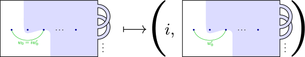
Figure 3.1: The Borel-Moore cycles considered in Lemma 3.11.

With these descriptions, we may now give the precise statement of the lemma.

Lemma 3.11 (“Cloud lemma”.)

For any choices of $w_{0}=iw^{\prime}_{0}$ and $\alpha$ as above, the module isomorphism (3.5) sends the element $[\alpha\times\beta]$ to the element $(i,[\alpha\times\beta^{\prime}])$, where $\beta$ and $\beta^{\prime}$ are determined by $w_{0}$ as described earlier.

Proof.

Let us write $\mathbf{w}=(w_{0},w_{1},\ldots,w_{g_{S}+n-1})\vdash\mathbf{k}$ and define an operation $(-)^{\prime\prime}$ on such tuples of words by setting $\mathbf{w}^{\prime\prime}=(w^{\prime\prime}_{0},w_{1},\ldots,w_{g_{S}+n-1})$, where $w_{0}=jw^{\prime\prime}_{0}$; in other words the operation $(-)^{\prime\prime}$ removes the first letter of the first word of $\mathbf{w}$. Note that $\mathbf{w}^{\prime\prime}\vdash\mathbf{k}_{j}$. For the sake of clarity, we prefer in this proof to denote by $e_{\mathbf{w}}$ (rather than $\mathbf{w}$) the standard basis element corresponding to the tuple $\mathbf{w}$, depicted in Figure 2.2. Then we denote by $e^{\prime}_{\mathbf{w}}$ the corresponding dual basis element depicted in Figure 2.3. By definition, the isomorphism (3.5) takes $e_{\mathbf{w}}$ to the element $e_{\mathbf{w}^{\prime\prime}}$ in the $j$th summand of the right-hand side.

Let us first decompose the element represented by the left-hand side of Figure 3.1 as

$$\sum_{\mathbf{w}\vdash\mathbf{k}}e_{\mathbf{w}}.\lambda_{\mathbf{w}}=\sum_{j=1}^{r}\sum_{\begin{subarray}{c}\mathbf{w}\vdash\mathbf{k}\\ w_{0}=jw^{\prime\prime}_{0}\end{subarray}}e_{\mathbf{w}}.\lambda_{\mathbf{w}},$$ (3.6)

where $\lambda_{\mathbf{w}}=\langle\mathrm{LHS},e^{\prime}_{\mathbf{w}}\rangle$ is the value of the intersection pairing (2.10) evaluated on the left-hand side of Figure 3.1 and the dual basis element $e^{\prime}_{\mathbf{w}}$. This is illustrated on the left-hand side of Figure 3.2. From that figure, it is clear that $\lambda_{\mathbf{w}}=0$ unless $j=i$, so we may remove the outer sum and set $j=i$ in the formula (3.6). Its image under the map (3.5) is

$$\sum_{\begin{subarray}{c}\mathbf{w}\vdash\mathbf{k}\\ w_{0}=iw^{\prime\prime}_{0}\end{subarray}}e_{\mathbf{w}^{\prime\prime}}.\lambda_{\mathbf{w}}.$$ (3.7)

On the other hand, the element represented by the right-hand side of Figure 3.1 decomposes as

$$\sum_{\mathbf{v}\vdash\mathbf{k}_{i}}e_{\mathbf{v}}.\mu_{\mathbf{v}},$$ (3.8)

where $\mu_{\mathbf{v}}=\langle\mathrm{RHS},e^{\prime}_{\mathbf{v}}\rangle$ is the value of the intersection pairing (2.10) evaluated on the right-hand side of Figure 3.1 and the dual basis element $e^{\prime}_{\mathbf{v}}$. This is illustrated on the right-hand side of Figure 3.2. There is clearly a bijection between the two indexing sets of the sums above given by sending $\mathbf{w}$ to $\mathbf{v}=\mathbf{w}^{\prime\prime}$. Thus, in order to prove that $\eqref{eq:cloud-lemma-LHS-image}=\eqref{eq:cloud-lemma-RHS}$, as desired, it remains to show that we have an equality of coefficients: $\langle\mathrm{LHS},e^{\prime}_{\mathbf{w}}\rangle=\lambda_{\mathbf{w}}=\mu_{\mathbf{w}^{\prime\prime}}=\langle\mathrm{RHS},e^{\prime}_{\mathbf{w}^{\prime\prime}}\rangle$.

To explain this, we briefly recall some of the details of how the intersection pairings $\langle\mathrm{LHS},e^{\prime}_{\mathbf{w}}\rangle$ and $\langle\mathrm{RHS},e^{\prime}_{\mathbf{w}^{\prime\prime}}\rangle$ may be computed; for more precise details, see [Big01, §2.1] or [PS22, §4.3] (when the surface is a disc) or [BPS21, §7] (for more general orientable surfaces).

We first consider $\langle\mathrm{LHS},e^{\prime}_{\mathbf{w}}\rangle$. We may assume without loss of generality that the Borel-Moore homology class denoted by $\mathrm{LHS}$ (the left-hand side of Figure 3.1) is represented by configuration spaces on a collection of pairwise disjoint properly-embedded arcs, one of these being the arc depicted and the others being contained in the shaded “cloud”. Indeed, this is due to the basis that we have described in §2. The dual basis element $e^{\prime}_{\mathbf{w}}$ is represented by the cycle given by the red vertical (and horizontal, in the handles) arcs on the left-hand side of Figure 3.2. We assume that these intersect the arcs representing $\mathrm{LHS}$ transversely, in particular in finitely many points.

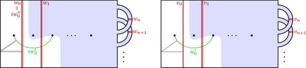
Figure 3.2: An illustration of the intersection pairings $\lambda_{\mathbf{w}}=\langle\mathrm{LHS},e^{\prime}_{\mathbf{w}}\rangle$ (left) and $\mu_{\mathbf{w}^{\prime\prime}}=\langle\mathrm{RHS},e^{\prime}_{\mathbf{w}^{\prime\prime}}\rangle$ (right). Here, $\mathrm{LHS}$ and $\mathrm{RHS}$ refer to the Borel-Moore homology classes depicted on the left-hand side and right-hand side of Figure 3.1 respectively.

The value of the pairing $\langle\mathrm{LHS},e^{\prime}_{\mathbf{w}}\rangle\in\mathbb{Z}[Q^{\star}_{(\mathbf{k},\ell)}(S)]$ is then a sum of terms $\epsilon_{p}\phi_{(\mathbf{k},\ell)}(\gamma_{p})$ indexed by these intersection points $p$, where $\epsilon_{p}\in\{\pm 1\}$ is a sign, $\gamma_{p}$ is a based loop in the configuration space $C_{\mathbf{k}}(\mathbb{D}_{1+n}\natural S)$ and $\phi_{(\mathbf{k},\ell)}\colon\pi_{1}(C_{\mathbf{k}}(\mathbb{D}_{1+n}\natural S))\to Q^{\star}_{(\mathbf{k},\ell)}(S)$ is the homomorphism determining the local system in the definition of $\mathfrak{L}^{\star}_{(\mathbf{k},\ell)}$ (see §1.2.3). More concretely, $\phi_{(\mathbf{k},\ell)}(\gamma_{p})$ is a tuple of integers counting various winding numbers of configuration points around the punctures of $\mathbb{D}_{1+n}\natural S$ and around each other during the loop $\gamma_{p}$. To determine $\gamma_{p}$, one must first of all choose a path from the base configuration to some point $x$ on (the cycle representing the homology class) $\mathrm{LHS}$ and another path from the base configuration to some point $y$ on (the cycle representing the homology class) $e^{\prime}_{\mathbf{w}}$. Such choices of “tethers” are in fact necessary to fully describe the homology classes that we are considering. However, different choices correspond to homology classes that differ only by unit scalars in the ground ring, so the choice does not matter for us, since (3.5) is a module morphism. We will assume, for convenience, that the parts of the tethers attached to the left-most arcs are as depicted in Figure 3.2. Given these choices, the loop $\gamma_{p}$ is then a concatenation of four paths

$$*\rightsquigarrow x\rightsquigarrow p\rightsquigarrow y\rightsquigarrow*$$

where the first and last are the tethers, the second is any path in $\mathrm{LHS}$ from $x$ to the intersection point $p$ and the third is any path in $e^{\prime}_{\mathbf{w}}$ from $p$ to $y$.

The intersection pairing $\langle\mathrm{RHS},e^{\prime}_{\mathbf{w}^{\prime\prime}}\rangle$ has an almost identical description, the only difference being that one red vertical arc (containing a single point in the $i$th block of the partition $\mathbf{k}$) has been removed and the green arc labelled by $iw^{\prime}_{0}$ is now labelled by $w^{\prime}_{0}$, so its left-most point (in the $i$th block of the partition $\mathbf{k}$) has also been removed.

To compare these two elements of $\mathbb{Z}[Q^{\star}_{(\mathbf{k},\ell)}(S)]$, first notice that there is a bijection of intersection points $\mathrm{RHS}\cap e^{\prime}_{\mathbf{w}^{\prime\prime}}\to\mathrm{LHS}\cap e^{\prime}_{\mathbf{w}}$ given by $p\mapsto\bar{p}=p\cup\{p_{0}\}$, where $p_{0}\in\mathbb{D}_{1+n}\natural S$ is the unique intersection point between the left-most vertical arc and the curved (green) arc on the left-hand side of Figure 3.2. It therefore suffices to check that we have $\epsilon_{\bar{p}}=\epsilon_{p}$ and $\phi_{(\mathbf{k},\ell)}(\gamma_{\bar{p}})=\phi_{(\mathbf{k},\ell)}(\gamma_{p})$, where the values with a subscript $\bar{p}$ are computed using the left-hand side of Figure 3.2 and those with a subscript $p$ are computed using the right-hand side of Figure 3.2.

The loop $\gamma_{\bar{p}}$ lies in a configuration space with one more point than the configuration space containing the loop $\gamma_{p}$. The key observation is that – up to basepoint-preserving homotopy – $\gamma_{\bar{p}}$ is obtained from $\gamma_{p}$ by simply adjoining a stationary point in the boundary of the surface. This fact may be read off directly, using the description above of how the loops are constructed, by comparing the two sides of Figure 3.2. In particular, no winding numbers are changed by adjoining this additional stationary point, so $\phi_{(\mathbf{k},\ell)}(\gamma_{\bar{p}})=\phi_{(\mathbf{k},\ell)}(\gamma_{p})$.

Finally, we recall that the sign $\epsilon_{p}$ is the product of the local signs of the intersections of arcs in the surface at each point of $p=\{p_{1},\ldots,p_{k}\}$ together with an additional sign recording the parity of the permutation of the base configuration induced by $\gamma_{p}$. The local sign of the intersection at $p_{0}$ is $+1$, so adjoining $p_{0}$ does not change the product of the local signs. In addition, as a consequence of the paragraph above, the permutation induced by $\gamma_{\bar{p}}$ is obtained from the permutation induced by $\gamma_{p}$ by adjoining a fixed point; in particular they both have the same parity. Thus $\epsilon_{\bar{p}}=\epsilon_{p}$. ∎

A decomposition property.

We also will need the following (easier) diagrammatic facts in §3.2.2–§3.2.3. This is an identity taking place in the Borel-Moore homology group $\mathfrak{L}^{\star}_{(\mathbf{k},\ell)}(S)(\mathtt{n})=H_{k}^{\mathrm{BM}}(C_{\mathbf{k}}(\mathbb{D}_{n}\natural S);\mathbb{Z}[Q^{\star}_{(\mathbf{k},\ell)}(S)])$ depicted in Figure 3.3.

The left-hand side of the figure represents a Borel-Moore cycle on $C_{\mathbf{k}}(\mathbb{D}_{n}\natural S)$ defined as follows. Choose a word $w$ on the alphabet $\{1,\ldots,r\}$ and write $\mathbf{j}=\boldsymbol{\{}j_{1};\ldots;j_{r}\boldsymbol{\}}$ where $j_{i}$ denotes the number of copies of the letter $i$ in $w$. Choose any cycle $\xi$ on $C_{\mathbf{k}-\mathbf{j}}(\mathbb{D}_{n}\natural S)$ supported in the blue shaded region and let $\omega$ denote the cycle on $C_{\mathbf{j}}(\mathbb{D}_{n}\natural S)$ given by the open singular simplex consisting of all configurations lying on the open green arc labelled according to the word $w$. Then $\xi\times\omega$ is the cycle depicted on the left-hand side.

The right-hand side of the figure represents a sum of classes, taken over all possible decompositions of the word $w$ into two words $w=w_{1}w_{2}$. The class in this sum corresponding to $(w_{1},w_{2})$ is $\xi\times\omega^{\prime}$, where $\xi$ is the previously-chosen cycle and $\omega^{\prime}$ is the cycle on $C_{\mathbf{j}}(\mathbb{D}_{n}\natural S)$ given by the open singular simplex consisting of all configurations lying on the two open green arcs labelled according to the words $w_{1}$ and $w_{2}$ respectively.

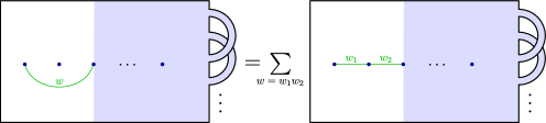
Figure 3.3: The identity of Lemma 3.12 in the orientable case. The identity in the non-orientable case is the obvious analogue; only the left-hand side of each diagram, which is planar, is important.

Lemma 3.12

For any choices of a cycle $\xi$ and a word $w$, defining the cycles $\omega$ and $\omega^{\prime}$ as described above, we have the relation $[\xi\times\omega]=\sum_{w=w_{1}w_{2}}[\xi\times\omega^{\prime}]$ in $\mathfrak{L}^{\star}_{(\mathbf{k},\ell)}(S)(\mathtt{n})$.

Proof.

We follow the notation of the proof of Lemma 3.11. The result follows immediately by verifying that each side of the equation evaluates to the same element of the ground ring when applying the intersection pairing $\langle-,e^{\prime}_{\mathbf{v}}\rangle$ with the dual basis element $e^{\prime}_{\mathbf{v}}$ for each $\mathbf{v}=(v_{1},v_{2},v_{3}\ldots)\vdash\mathbf{k}$. (Details of how these intersection pairings are computed are explained in the proof of Lemma 3.11 above.) ∎

3.2.2 For classical braid groups

Our aim here is to prove Theorem B for each $(\mathbf{k},\ell)$-Lawrence-Bigelow functor $\mathfrak{LB}_{(\mathbf{k},\ell)}$ and its untwisted version $\mathfrak{LB}^{u}_{(\mathbf{k},\ell)}$ of §1.3.1, i.e. for the homological representation functors of §3.2.1 with $S=\mathbb{D}$. The arguments for this are exactly the same for both $\mathfrak{LB}_{(\mathbf{k},\ell)}$ and $\mathfrak{LB}^{u}_{(\mathbf{k},\ell)}$. So, following Notation 1.6 and §3.2.1, we henceforth speak of the functor $\mathfrak{LB}^{\star}_{(\mathbf{k},\ell)}$ where $\star$ either stands for the blank space or $\star=u$. We also define the following Lawrence-Bigelow functors for the parameter $k=0$, noting that this convention differs from the general convention of Notation 3.3:

Notation 3.13

We denote by $\mathfrak{LB}_{(0,\ell)}\colon\langle\boldsymbol{\beta},\boldsymbol{\beta}\rangle\to{\mathbb{Z}[Q_{((1),\ell)}(\mathbb{D})]}{}\textrm{-}\mathrm{Mod}$ the subobject of the constant functor at $\mathbb{Z}[Q_{((1),\ell)}(\mathbb{D})]$ with $\mathfrak{LB}_{(0,\ell)}(\mathtt{0})=\mathfrak{LB}_{(0,\ell)}(\mathtt{1})=0$ and $\mathfrak{LB}_{(0,\ell)}(\mathtt{n})=\mathbb{Z}[Q_{((1),\ell)}(\mathbb{D})]$ for $\mathtt{n}\geqslant\mathtt{2}$. This choice is driven by consistency with the definition of the Lawrence-Bigelow functors, because $\mathfrak{LB}_{(\mathbf{k},\ell)}(\mathtt{0})=\mathfrak{LB}_{(\mathbf{k},\ell)}(\mathtt{1})=0$.

For any $\mathtt{n}\in\mathrm{Obj}(\boldsymbol{\beta})$, we recall from the preliminary study of §3.2.1 that $\kappa_{\mathtt{1}}\mathfrak{LB}^{\star}_{(\mathbf{k},\ell)}(\mathtt{n})=0$ and $\delta_{\mathtt{1}}\mathfrak{LB}^{\star}_{(\mathbf{k},\ell)}(\mathtt{n})$ is the free $\mathbb{Z}[Q^{\star}_{(\mathbf{k},\ell)}(\mathbb{D})]$-module with basis given by the tuples $(w_{0},w_{1},\ldots,w_{n-1})\vdash\mathbf{k}$ such that $|w_{0}|\geqslant 1$, which identifies as a $\mathbb{Z}[Q^{\star}_{(\mathbf{k},\ell)}(\mathbb{D})]$-module to the direct sum $\bigoplus_{1\leqslant j\leqslant r}\tau_{\mathtt{1}}\mathfrak{LB}^{\star}_{(\mathbf{k}_{j},\ell)}(\mathtt{n})$ via the isomorphism (3.5) (if $\mathtt{n}\geqslant\mathtt{1}$; it is trivial otherwise). From now on, we denote this isomorphism by $(\mathfrak{p}_{(\mathbf{k},\ell)})_{\mathtt{n}}$, setting $(\mathfrak{p}_{(\mathbf{k},\ell)})_{\mathtt{0}}$ to be the null morphism. We now prove the main result of §3.2.2:

Theorem 3.14

For each $\mathbf{k}\vdash k\geqslant 1$ and $\ell\geqslant 1$, the exact sequence (3.1) induces the short exact sequences:

(3.9)

(3.10)

in $\mathbf{Fct}(\langle\boldsymbol{\beta},\boldsymbol{\beta}\rangle,{\mathbb{Z}[Q_{(\mathbf{k},\ell)}(\mathbb{D})]}{}\textrm{-}\mathrm{Mod}^{\bullet})$ and $\mathbf{Fct}(\langle\boldsymbol{\beta},\boldsymbol{\beta}\rangle,{\mathbb{Z}[Q^{u}_{(\mathbf{k},\ell)}(\mathbb{D})]}{}\textrm{-}\mathrm{Mod})$ respectively. Furthermore, the short exact sequences (3.9) and (3.10) still hold after any change of rings operation.

Proof.

The strategy consists in showing that the isomorphisms $\{(\mathfrak{p}_{(\mathbf{k},\ell)})_{\mathtt{n}}\}_{\mathtt{n}\in\mathrm{Obj}(\boldsymbol{\beta})}$ define an isomorphism $\mathfrak{p}_{(\mathbf{k},\ell)}\colon\delta_{\mathtt{1}}\mathfrak{LB}^{\star}_{(\mathbf{k},\ell)}\overset{\sim}{\to}\bigoplus_{1\leqslant j\leqslant r}\tau_{\mathtt{1}}\mathfrak{LB}^{\star}_{(\mathbf{k}_{j},\ell)}$ in $\mathbf{Fct}(\langle\boldsymbol{\beta},\boldsymbol{\beta}\rangle,{\mathbb{Z}[Q^{\star}_{(\mathbf{k},\ell)}(\mathbb{D})]}{}\textrm{-}\mathrm{Mod}^{\bullet})$.

We start by proving that assembling these isomorphisms of modules defines an isomorphism in the category $\mathbf{Fct}(\boldsymbol{\beta},{\mathbb{Z}[Q^{\star}_{(\mathbf{k},\ell)}(\mathbb{D})]}{}\textrm{-}\mathrm{Mod}^{\bullet})$, in other words that each $(\mathfrak{p}_{(\mathbf{k},\ell)})_{\mathtt{n}}$ is a $\mathbf{B}_{n}$-module morphism. The braid group $\mathbf{B}_{n}$ being trivial for $n\in\{0,1\}$, we consider $\mathtt{n}\geqslant\mathtt{2}$ and prove the commutation of $(\mathfrak{p}_{(\mathbf{k},\ell)})_{\mathtt{n}}$ with respect to the action of any Artin generator $\sigma_{i}$ of $\mathbf{B}_{n}$ with $1\leqslant i\leqslant n-1$. We recall from Proposition 2.4 that the morphisms $\tau_{\mathtt{1}}\mathfrak{LB}^{\star}_{(\mathbf{k}_{j},\ell)}(\sigma_{i})$ for all $1\leqslant j\leqslant r$ and $\delta_{\mathtt{1}}\mathfrak{LB}^{\star}_{(\mathbf{k},\ell)}(\sigma_{i})$ are defined by the action of the generator $\sigma_{i+1}$ on the Borel-Moore homology classes on the graph $\mathbb{I}_{1+n}$; see Figure 1(a) with $g=0$.

For $i=1$, we note that the actions of $\tau_{\mathtt{1}}\mathfrak{LB}^{\star}_{(\mathbf{k}_{j},\ell)}(\sigma_{1})$ and of $\delta_{\mathtt{1}}\mathfrak{LB}^{\star}_{(\mathbf{k},\ell)}(\sigma_{1})$ on the basis elements $(w^{\prime}_{0},\ldots,w_{n})$ and $(jw^{\prime}_{0},\ldots,w_{n})$ are illustrated, respectively, by the right-hand side and left-hand side of Figure 3.1 (with $g=0$). Namely, by the choice of Convention 1.3, the labelled green arc is the image of the left-most edge of the graph $\mathbb{I}_{1+n}$, denoted $(1,2)$ (using the obvious enumeration of its vertices), under the action of $\sigma_{2}$, which swaps the points $2$ and $3$ anticlockwise, while the other edges are concentrated in the blue shaded region. It thus follows from Lemma 3.11 and the definition of $(\mathfrak{p}_{(\mathbf{k},\ell)})_{\mathtt{n}}$ that $(\mathfrak{p}_{(\mathbf{k},\ell)})_{\mathtt{n}}\circ\delta_{\mathtt{1}}\mathfrak{LB}^{\star}_{(\mathbf{k},\ell)}(\mathtt{n})(\sigma_{1})=(\bigoplus_{1\leqslant j\leqslant r}\tau_{\mathtt{1}}\mathfrak{LB}^{\star}_{(\mathbf{k}_{j},\ell)}(\sigma_{1}))\circ(\mathfrak{p}_{(\mathbf{k},\ell)})_{\mathtt{n}}$.

For $i\geqslant 2$, we note that $\sigma_{i+1}$ acts trivially on the parts of the cycles representing the basis elements $(w^{\prime}_{0},\ldots,w_{n-1})$ and $(jw^{\prime}_{0},\ldots,w_{n-1})$ corresponding to the words $w^{\prime}_{0}$ and $jw^{\prime}_{0}$. Indeed, the action of $\sigma_{i+1}$ is supported in the subsurface containing the subgraph $\mathbb{I}_{n}\subset\mathbb{I}_{1+n}$, but excluding the left-most edge $(1,2)$, where the parts of the cycles corresponding to the words $w^{\prime}_{0}$ and $jw^{\prime}_{0}$ are supported. It follows by definition of $(\mathfrak{p}_{(\mathbf{k},\ell)})_{\mathtt{n}}$ (see (3.4)) that we have $(\mathfrak{p}_{(\mathbf{k},\ell)})_{\mathtt{n}}\circ\delta_{\mathtt{1}}\mathfrak{LB}^{\star}_{(\mathbf{k},\ell)}(\mathtt{n})(\sigma_{i})=(\bigoplus_{1\leqslant j\leqslant r}\tau_{\mathtt{1}}\mathfrak{LB}^{\star}_{(\mathbf{k}_{j},\ell)}(\sigma_{i}))\circ(\mathfrak{p}_{(\mathbf{k},\ell)})_{\mathtt{n}}$ for $i\geqslant 2$. (To be meticulous, this also uses a (simpler) analogue of Lemma 3.11, similarly to the case of $i=1$ above.) We have thus verified that $\mathfrak{p}_{(\mathbf{k},\ell)}$ is a natural transformation in $\mathbf{Fct}(\boldsymbol{\beta},{\mathbb{Z}[Q^{\star}_{(\mathbf{k},\ell)}(\mathbb{D})]}{}\textrm{-}\mathrm{Mod}^{\bullet})$.

We now prove that $\mathfrak{p}_{(\mathbf{k},\ell)}$ is a natural transformation in $\mathbf{Fct}(\langle\boldsymbol{\beta},\boldsymbol{\beta}\rangle,{\mathbb{Z}[Q^{\star}_{(\mathbf{k},\ell)}(\mathbb{D})]}{}\textrm{-}\mathrm{Mod}^{\bullet})$ via the strategy of Lemma 1.2. We fix an integer $\mathtt{n}\geqslant\mathtt{1}$, the proof being trivial for $\mathtt{n}=\mathtt{0}$. We note from (1.1) that $\tau_{\mathtt{1}}\mathfrak{LB}^{\star}_{(\mathbf{k},\ell)}([\mathtt{1},\mathrm{id}_{\mathtt{1}\natural\mathtt{n}}])=\mathfrak{LB}^{\star}_{(\mathbf{k},\ell)}(\sigma_{1}^{-1})\circ\mathfrak{LB}^{\star}_{(\mathbf{k},\ell)}([\mathtt{1},\mathrm{id}_{\mathtt{2}\natural\mathtt{n}}])$. (Here, we recall from §1.1.2.2 that we have the canonical identification $\sigma_{1}=b_{\mathtt{1},\mathtt{1}}^{\boldsymbol{\beta}}\natural\mathrm{id}_{\mathtt{n}}$ defined by the braiding $b_{\mathtt{1},\mathtt{1}}^{\boldsymbol{\beta}}\colon\mathtt{1}\natural\mathtt{1}\cong\mathtt{1}\natural\mathtt{1}$.)

We deduce from the description of $\mathfrak{LB}^{\star}_{(\mathbf{k},\ell)}([\mathtt{1},\mathrm{id}_{\mathtt{1}\natural\mathtt{n}}])$ in §3.2.1 that the map $\mathfrak{LB}^{\star}_{(\mathbf{k},\ell)}([\mathtt{1},\mathrm{id}_{\mathtt{2}\natural\mathtt{n}}])$ is the morphism induced by the embedding of $\mathbb{I}_{1+n}$ into $\mathbb{I}_{2+n}$ defined by sending each edge $(i,i+1)$ for $1\leqslant i\leqslant n$ to the edge $(i+1,i+2)$. Hence there are no configuration points on the left-most edge $(1,2)$ of $\mathbb{I}_{2+n}$ in the image of $\mathfrak{LB}^{\star}_{(\mathbf{k},\ell)}([\mathtt{1},\mathrm{id}_{\mathtt{2}\natural\mathtt{n}}])$. Also, the morphism $\mathfrak{LB}^{\star}_{(\mathbf{k},\ell)}(\sigma_{1}^{-1})$ is defined by the action of $\sigma_{1}^{-1}$ on $\mathbb{I}_{2+n}$ as illustrated on the left-hand side of Figure 3.3. For each $1\leqslant j\leqslant r$, we thus deduce from Lemma 3.12 that $((\mathfrak{p}_{(\mathbf{k},\ell)})_{\mathtt{1}\natural\mathtt{n}}\circ\delta_{\mathtt{1}}\mathfrak{LB}^{\star}_{(\mathbf{k},\ell)}([\mathtt{1},\mathrm{id}_{\mathtt{1}\natural\mathtt{n}}]))(jw^{\prime}_{0},\ldots,w_{n})$ and $\tau_{\mathtt{1}}\mathfrak{LB}^{\star}_{(\mathbf{k}_{j},\ell)}(\mathtt{n})([\mathtt{1},\mathrm{id}_{\mathtt{1}\natural\mathtt{n}}])(w^{\prime}_{0},\ldots,w_{n})$ are both equal to $\sum_{u_{0}v_{0}=w^{\prime}_{0}}(u_{0},v_{0},w_{1},\ldots,w_{n})$.

Therefore, it follows from the definition of $(\mathfrak{p}_{(\mathbf{k},\ell)})_{\mathtt{n}}$ and induction on $\mathtt{m}$ (the base case $\mathtt{m}=\mathtt{1}$ being the previous paragraph) that $(\bigoplus_{1\leqslant j\leqslant r}\tau_{\mathtt{1}}\mathfrak{LB}^{\star}_{(\mathbf{k}_{j},\ell)}([\mathtt{m},\mathrm{id}_{\mathtt{m}\natural\mathtt{n}}]))\circ(\mathfrak{p}_{(\mathbf{k},\ell)})_{\mathtt{n}}$ is equal to $(\mathfrak{p}_{(\mathbf{k},\ell)})_{\mathtt{m}\natural\mathtt{n}}\circ\delta_{\mathtt{1}}\mathfrak{LB}^{\star}_{(\mathbf{k},\ell)}([\mathtt{m},\mathrm{id}_{\mathtt{m}\natural\mathtt{n}}])$. Hence Relation (1.3) is satisfied for all $\mathtt{n}\geqslant\mathtt{1}$, which implies, by Lemma 1.2, that $\mathfrak{p}_{(\mathbf{k},\ell)}$ is a natural transformation (indeed, a natural isomorphism) on $\langle\boldsymbol{\beta},\boldsymbol{\beta}\rangle$. This provides the short exact sequences (3.9) and (3.10) of functors on $\langle\boldsymbol{\beta},\boldsymbol{\beta}\rangle$.

In the above arguments, whenever we consider a twisted homological representation functor, we stress that the associated action of $\delta_{\mathtt{1}}\mathfrak{LB}^{\star}_{(\mathbf{k},\ell)}$ on the ground ring $\mathbb{Z}[Q^{\star}_{(\mathbf{k},\ell)}(\mathbb{D})]$ does not affect the reasoning, since $\bigoplus_{1\leqslant j\leqslant r}\tau_{\mathtt{1}}\mathfrak{LB}^{\star}_{(\mathbf{k}_{j},\ell)}$ is automatically equipped with the same action via the implicit change of rings of Convention 3.7 for each summand; see Observation 3.6.

The fact that the short exact sequences (3.9) and (3.10) still hold after any change of rings operation follows from Lemma 3.8. ∎

Remark 3.15

There is no obvious splitting for the short exact sequences of functors (3.9) and (3.10). For instance, there is an obvious splitting of (3.9) at the level of modules given by sending each basis element $(w_{0},\ldots,w_{n})\in\tau_{\mathtt{1}}\mathfrak{LB}_{(\mathbf{k}_{j},\ell)}(\mathtt{n})$ for $1\leqslant j\leqslant r$ to $(jw_{0},\ldots,w_{n})$. However, one may check that this splitting does not commute with the action of $\sigma_{1}$; in particular it is not a natural transformation of functors on $\langle\boldsymbol{\beta},\boldsymbol{\beta}\rangle$.

3.2.3 For braid groups on surfaces different from the disc

We deal here with the short exact sequences for the homological representation functors $\mathfrak{L}_{(\mathbf{k},\ell)}(\Sigma_{g,1})$, $\mathfrak{L}^{u}_{(\mathbf{k},\ell)}(\Sigma_{g,1})$, $\mathfrak{L}_{(\mathbf{k},\ell)}(\mathscr{N}_{h,1})$ and $\mathfrak{L}^{u}_{(\mathbf{k},\ell)}(\mathscr{N}_{h,1})$ of §1.3.2 for any $\mathbf{k}\vdash k\geqslant 1$, $\ell\geqslant 1$, $g\geqslant 1$ and $h\geqslant 1$; see Theorem 3.19. The arguments for our work in this section are analogous regardless of which of the homological representation functors amongst this list we consider. For the sake of simplicity and to avoid repetition, we thus pool the key steps and common arguments for the remainder of §3.2.3, only emphasising the (minor) differences when necessary. Following Notation 1.6 and §3.2.1, we use the standard notation $\mathfrak{L}^{\star}_{(\mathbf{k},\ell)}(S)$, where $\star$ either stands for the blank space or $\star=u$, $S$ is either $\Sigma_{g,1}$ or $\mathscr{N}_{h,1}$ with $g,h\geqslant 1$, $Q^{\star}_{(\mathbf{k},\ell)}(S)$ is the associated transformation group and $\boldsymbol{\beta}^{S}$ is the associated groupoid.

Furthermore, it will be convenient to consider various “cut versions” of these homological representation functors defined on $\langle\boldsymbol{\beta},\boldsymbol{\beta}^{S}\rangle$. In fact, this definition makes sense more generally:

Definition 3.16 (Cut functors.)

Let $\mathcal{C}$ be a category whose objects form a totally-ordered set and in which there are no morphisms $a\to b$ if $a>b$. For such a category $\mathcal{C}$, a functor $F\colon\mathcal{C}\to R{}\textrm{-}\mathrm{Mod}$ and an object $c$ of $\mathcal{C}$, we define the truncation $F_{\mid\geqslant c}\colon\mathcal{C}\to R{}\textrm{-}\mathrm{Mod}$ on objects by $F_{\mid\geqslant c}(a)=F(a)$ for $a\geqslant c$ and $F_{\mid\geqslant c}(a)=0$ for $a<c$ and on morphisms by $F_{\mid\geqslant c}(f)=F(f)$ if the domain of $f$ is $\geqslant c$ and $F_{\mid\geqslant c}(f)=0$ otherwise.

In the case of $\mathcal{C}=\langle\boldsymbol{\beta},\boldsymbol{\beta}^{S}\rangle$, the objects form the totally-ordered set $\mathbb{N}$. This “cut” alteration is negligible for our later study of polynomiality (see the proof of Corollary C for surface braid groups in §4.2), while the “cut” subfunctors are much more convenient to deal with (see Remark 3.21).

We recall from the preliminary study of §3.2.1 that $\kappa_{\mathtt{1}}\mathfrak{L}^{\star}_{(\mathbf{k},\ell)}(S)(\mathtt{n})=0$ and that $\delta_{\mathtt{1}}\mathfrak{L}^{\star}_{(\mathbf{k},\ell)}(S)(\mathtt{n})$ is the free $\mathbb{Z}[Q^{\star}_{(\mathbf{k},\ell)}(S)]$-module with basis given by the tuples of words $(w_{0},w_{1},\ldots,w_{g_{S}+n-1})\vdash\mathbf{k}$ such that $|w_{0}|\geqslant 1$ for each $\mathtt{n}\in\mathrm{Obj}(\boldsymbol{\beta}^{S})$. For $\mathtt{n}\geqslant\mathtt{2}$, we denote by $(\mathfrak{p}_{(\mathbf{k},\ell)})_{\mathtt{n}}$ the $\mathbb{Z}[Q^{\star}_{(\mathbf{k},\ell)}(S)]$-module isomorphism (3.5), which may be written as

$$\delta_{\mathtt{1}}\mathfrak{L}^{\star}_{(\mathbf{k},\ell)\mid\geqslant 2}(S)(\mathtt{n})\overset{\cong}{\longrightarrow}\underset{1\leqslant j\leqslant r}{\bigoplus}(\tau_{\mathtt{1}}\mathfrak{L}^{\star}_{(\mathbf{k}_{j},\ell)}(S))_{\mid\geqslant 2}(\mathtt{n})$$ (3.11)

since the truncations do not make any difference when $\mathtt{n}\geqslant\mathtt{2}$. We also set $(\mathfrak{p}_{(\mathbf{k},\ell)})_{\mathtt{0}}$ to be the trivial morphism; this gives an isomorphism of the form (3.11) for $\mathtt{n}=\mathtt{0}$. However, for $\mathtt{n}=\mathtt{1}$ there is no isomorphism of the form (3.11), since the right-hand side is zero, whereas we have $\delta_{\mathtt{1}}\mathfrak{L}^{\star}_{(\mathbf{k},\ell)\mid\geqslant 2}(S)(\mathtt{1})\cong\tau_{\mathtt{1}}\mathfrak{L}^{\star}_{(\mathbf{k},\ell)\mid\geqslant 2}(S)(\mathtt{1})$ as $\mathbf{B}_{1}(S)$-representations over $\mathbb{Z}[Q^{\star}_{(\mathbf{k},\ell)}(S)]$.

Our first goal in this section is to promote (3.11) to a natural isomorphism of functors on $\langle\boldsymbol{\beta},\boldsymbol{\beta}^{S}\rangle$, so we first need to correct the right-hand side on the object $\mathtt{n}=\mathtt{1}$. To do this, we choose a certain extension of functors, via the following lemma:

Lemma 3.17

Let $\mathcal{M}$ be a module over a braided monoidal groupoid $\mathcal{G}$ that on objects is given by the monoid $\mathbb{N}$ as a module over itself. Let $F,G\colon\langle\mathcal{G},\mathcal{M}\rangle\to R{}\textrm{-}\mathrm{Mod}$ be two functors with $F(n)=0$ for $n\leqslant c-1$ and $G(n)=0$ for $n\geqslant c$ for an integer $c\geqslant 1$. Then there is a one-to-one correspondence between extensions of $G$ by $F$, i.e. short exact sequences $0\to F\to{?}\to G\to 0$, and morphisms $G(c-1)\to F(c)$ in $R{}\textrm{-}\mathrm{Mod}$, given by evaluating the extension functor at $[\mathtt{1},\mathrm{id}_{c}]$.

Proof.

Since $F$ and $G$ have disjoint support, there is no choice about the action of any such extension on objects and on automorphisms; in other words, there is a unique extension of $G$ by $F$ when restricting the domain to the subgroupoid $\mathcal{G}$. Lemma 1.1 describes the data and conditions required to extend a functor on $\mathcal{G}$ to a functor on $\langle\mathcal{G},\mathcal{M}\rangle$. In light of the requirement that this is an extension of $G$ by $F$, the only remaining choice is the value assigned to the morphism $[\mathtt{1},\mathrm{id}_{c}]$; conversely, any such choice determines an extension. ∎

Definition 3.18 (An extension by an atomic functor.)

Denote by $\tau_{\mathtt{1}}\mathfrak{L}^{\star}_{(\mathbf{k},\ell)\mid\geqslant 2}(S)(\mathtt{1})$ the “atomic” functor on $\langle\boldsymbol{\beta},\boldsymbol{\beta}^{S}\rangle$ whose value on the object $\mathtt{1}$ is $\tau_{\mathtt{1}}\mathfrak{L}^{\star}_{(\mathbf{k},\ell)\mid\geqslant 2}(S)(\mathtt{1})$ and whose value on all other objects is the zero module. Denote by $\widetilde{\bigoplus}_{1\leqslant j\leqslant r}(\tau_{\mathtt{1}}\mathfrak{L}^{\star}_{(\mathbf{k}_{j},\ell)}(S))_{\mid\geqslant 2}$ the unique extension of this atomic functor by the functor $\bigoplus_{1\leqslant j\leqslant r}(\tau_{\mathtt{1}}\mathfrak{L}^{\star}_{(\mathbf{k}_{j},\ell)}(S))_{\mid\geqslant 2}$ whose value on $[\mathtt{1},\mathrm{id}_{\mathtt{2}}]$ is:

We also denote by $(\mathfrak{p}_{(\mathbf{k},\ell)})_{1}$ the isomorphism

(3.12)

Using the extension of Definition 3.18, we may now upgrade (3.11) to an isomorphism of functors:

Theorem 3.19

For any $S=\Sigma_{g,1}\text{ or }\mathscr{N}_{h,1}$, $\mathbf{k}\vdash k\geqslant 1$ and $\ell\geqslant 1$, the exact sequence (3.1) induces a short exact sequence

(3.13)

of functors in

• $\mathbf{Fct}(\langle\boldsymbol{\beta},\boldsymbol{\beta}^{S}\rangle,\mathbb{Z}[Q_{(\mathbf{k},\ell)}(S)]{}\textrm{-}\mathrm{Mod})$ if $\ell\leqslant 2$;

• $\mathbf{Fct}(\langle\boldsymbol{\beta},\boldsymbol{\beta}^{S}\rangle,\mathbb{Z}[Q^{u}_{(\mathbf{k},\ell)}(S)]{}\textrm{-}\mathrm{Mod})$ if $\ell\geqslant 3$ and $\star=u$;

• $\mathbf{Fct}(\langle\boldsymbol{\beta},\boldsymbol{\beta}^{S}\rangle,\mathbb{Z}{}\textrm{-}\mathrm{Mod})$ if $\ell\geqslant 3$ and $\star$ is the blank space.

These short exact sequences hold also after any change of rings operation.

Proof.

The roadmap of this proof is similar to that of Theorem 3.14, whose arguments are reused below for the analogous steps. As in the proof of Theorem 3.14, we stress that, when we deal with a twisted homological representation functor, the action on the ground ring $\mathbb{Z}[Q_{(\mathbf{k},\ell)}(S)]$ does not affect any point of the following work thanks to the implicit change of rings of Convention 3.7.

To prove the theorem, it will suffice to show that the module isomorphisms (3.11) and (3.12) assemble to an isomorphism of functors on $\langle\boldsymbol{\beta},\boldsymbol{\beta}^{S}\rangle$. As a first step, we show that they assemble to an isomorphism of functors on $\boldsymbol{\beta}^{S}$; in other words, that they are isomorphisms of $\mathbf{B}_{n}(S)$-representations for each $\mathtt{n}\geqslant\mathtt{1}$.

We first consider the case where $\mathtt{n}\geqslant\mathtt{2}$ and use the generating set for $\mathbf{B}_{n}(S)$ recalled in [PS23, Prop. 2.2]. For each generator $\rho\in\mathbf{B}_{n}(S)$, the morphisms $(\tau_{\mathtt{1}}\mathfrak{L}^{\star}_{(\mathbf{k}_{j},\ell)}(S))_{\mid\geqslant 2}(\rho)$ for all $1\leqslant j\leqslant r$ and $\delta_{\mathtt{1}}\mathfrak{L}^{\star}_{(\mathbf{k},\ell)\mid\geqslant 2}(S)(\rho)$ are induced by the action of $\mathrm{id}_{\mathtt{1}}\natural\rho$ on the Borel-Moore homology classes supported on the embedded graph $\mathbb{I}_{1+n}\vee\mathbb{W}^{S}\subset\mathbb{D}_{1+n}\natural S$.

If $\rho\neq\sigma_{1}$, the action of $\mathrm{id}_{\mathtt{1}}\natural\rho$ is supported on a subsurface containing the graph $\mathbb{I}_{n}\vee\mathbb{W}^{S}$ and disjoint from the left-most edge $(1,2)$. The action therefore does not affect the first entries of the basis elements $(w^{\prime}_{0},\ldots)$ and $(jw^{\prime}_{0},\ldots)$. Thus $(\tau_{\mathtt{1}}\mathfrak{L}^{\star}_{(\mathbf{k}_{j},\ell)}(S))_{\mid\geqslant 2}(\rho)$ does not interact with the action of $(\mathfrak{p}_{(\mathbf{k},\ell)})_{\mathtt{n}}$ and we have $(\mathfrak{p}_{(\mathbf{k},\ell)})_{\mathtt{n}}\circ\delta_{\mathtt{1}}\mathfrak{L}^{\star}_{(\mathbf{k},\ell)\mid\geqslant 2}(S)(\rho)=\bigl{(}\widetilde{\bigoplus}_{1\leqslant j\leqslant r}(\tau_{\mathtt{1}}\mathfrak{L}^{\star}_{(\mathbf{k}_{j},\ell)}(S))_{\mid\geqslant 2}(\rho)\bigr{)}\circ(\mathfrak{p}_{(\mathbf{k},\ell)})_{\mathtt{n}}$. Hence the only remaining fact to check is that this last equality also holds for $\sigma_{1}$: this is done by repeating verbatim the corresponding point in the proof of Theorem 3.14, using Lemma 3.11. Furthermore, the analogous relations trivially hold also for $\mathtt{n}=\mathtt{0}$ (because $\mathfrak{L}^{\star}_{(\mathbf{k},\ell)\mid\geqslant 2}(S)(\mathtt{0})=0$) and for $\mathtt{n}=\mathtt{1}$ (because the isomorphism $(\mathfrak{p}_{(\mathbf{k},\ell)})_{1}=\eqref{eq:isomorphism-in-degree-one}$ is $\mathbf{B}_{1}(S)$-equivariant by construction). Therefore, the collection of isomorphisms $\{(\mathfrak{p}_{(\mathbf{k},\ell)})_{\mathtt{n}}\}$ assembles into a natural isomorphism $\mathfrak{p}_{(\mathbf{k},\ell)}$ of functors on $\boldsymbol{\beta}^{S}$ from $\delta_{\mathtt{1}}\mathfrak{L}^{\star}_{(\mathbf{k},\ell)\mid\geqslant 2}(S)$ to $\widetilde{\bigoplus}_{1\leqslant j\leqslant r}(\tau_{\mathtt{1}}\mathfrak{L}^{\star}_{(\mathbf{k}_{j},\ell)}(S))_{\mid\geqslant 2}$.

Since the canonical inclusion $\boldsymbol{\beta}^{S}\hookrightarrow\langle\boldsymbol{\beta},\boldsymbol{\beta}^{S}\rangle$ is the identity on objects, to check that $\mathfrak{p}_{(\mathbf{k},\ell)}$ extends to a natural isomorphism of functors on $\langle\boldsymbol{\beta},\boldsymbol{\beta}^{S}\rangle$, it suffices to check certain additional relations. Specifically, by Lemma 1.2, it suffices to check Relation (1.3), which we do now. First, we note from (1.1) that $\tau_{\mathtt{1}}\mathfrak{L}^{\star}_{(\mathbf{k},\ell)\mid\geqslant 2}(S)([\mathtt{1},\mathrm{id}_{\mathtt{1}\natural\mathtt{n}}])=\mathfrak{L}^{\star}_{(\mathbf{k},\ell)\mid\geqslant 2}(S)(\sigma_{1}^{-1})\circ\mathfrak{L}^{\star}_{(\mathbf{k},\ell)\mid\geqslant 2}(S)([\mathtt{1},\mathrm{id}_{\mathtt{2}\natural\mathtt{n}}])$ (using the canonical identification $b_{\mathtt{1},\mathtt{1}}^{\boldsymbol{\beta}}\natural\mathrm{id}_{\mathtt{n}}=\sigma_{1}$). We recall from the description of $\mathfrak{L}^{\star}_{(\mathbf{k},\ell)}(S)([\mathtt{1},\mathrm{id}_{\mathtt{1}\natural\mathtt{n}}])$ in §3.2.1 that $\mathfrak{L}^{\star}_{(\mathbf{k},\ell)\mid\geqslant 2}(S)([\mathtt{1},\mathrm{id}_{\mathtt{2}\natural\mathtt{n}}])$ is induced by the embedding of $\mathbb{I}_{1+n}$ into $\mathbb{I}_{2+n}$ defined by sending each edge $(i,i+1)$ to the edge $(i+1,i+2)$ and by the identity on the wedge $\mathbb{W}^{S}$. Using Lemma 3.12 with the illustration of Figure 3.3, the analogous point in the proof of Theorem 3.14 repeats mutatis mutandis here. This proves that ${(\mathfrak{p}_{(\mathbf{k},\ell)})}_{\mathtt{m}\natural\mathtt{n}}\circ\delta_{\mathtt{1}}\mathfrak{L}^{\star}_{(\mathbf{k},\ell)\mid\geqslant 2}(S)([\mathtt{m},\mathrm{id}_{\mathtt{m}\natural\mathtt{n}}])=\left(\widetilde{\bigoplus}_{1\leqslant j\leqslant r}(\tau_{\mathtt{1}}\mathfrak{L}^{\star}_{(\mathbf{k}_{j},\ell)}(S))_{\mid\geqslant 2}([\mathtt{m},\mathrm{id}_{\mathtt{m}\natural\mathtt{n}}])\right)\circ(\mathfrak{p}_{(\mathbf{k},\ell)})_{\mathtt{n}}$ for each $\mathtt{m}\geqslant 1$ and $\mathtt{n}\geqslant\mathtt{2}$. The analogous relation follows in the exact same way for $\mathtt{n}=\mathtt{1}$, the point being that $\widetilde{\bigoplus}_{1\leqslant j\leqslant r}(\tau_{\mathtt{1}}\mathfrak{L}^{\star}_{(\mathbf{k}_{j},\ell)}(S))_{\mid\geqslant 2}([\mathtt{1},\mathrm{id}_{\mathtt{2}}])=\delta_{\mathtt{1}}\mathfrak{L}_{(\mathbf{k},\ell)\mid\geqslant 2}^{\star}([\mathtt{1},\mathrm{id}_{\mathtt{2}}])\circ\Delta_{\mathtt{1}}\mathfrak{L}_{(\mathbf{k},\ell)\mid\geqslant 2}^{\star}(\mathtt{1})$. In addition, this relation also holds trivially for $\mathtt{n}=\mathtt{0}$ because $\mathfrak{L}^{\star}_{(\mathbf{k},\ell)\mid\geqslant 2}(S)(\mathtt{0})=0$. Hence Relation (1.3) is satisfied for each $\mathtt{n}\in\mathrm{Obj}(\boldsymbol{\beta}^{S})$, so Lemma 1.2 implies that the isomorphisms $(\mathfrak{p}_{(\mathbf{k},\ell)})_{\mathtt{n}}=\text{\eqref{eq:isom-of-modules-truncated} and \eqref{eq:isomorphism-in-degree-one}}$ assemble to an isomorphism of functors on $\langle\boldsymbol{\beta},\boldsymbol{\beta}^{S}\rangle$, as desired.

Finally, the fact that the short exact sequences (3.13) hold also after any change of rings operation follows from Lemma 3.8. ∎

Remark 3.20

Similarly to Remark 3.15, we note that there is no obvious splitting for the short exact sequence of functors (3.13).

Remark 3.21

We conjecture that Theorem 3.19 holds also for the functors $\mathfrak{L}^{\star}_{(\mathbf{k},\ell)}(S)$, i.e., without truncating to the functors $\mathfrak{L}^{\star}_{(\mathbf{k},\ell)\mid\geqslant 2}(S)$ via Definition 3.16. By the arguments of §4 below it would then follow that that these non-truncated functors are strong and weak polynomial with the same degrees as the truncated ones. For the trivial partition $\mathbf{k}=(k)$, we have verified this for the functor $\mathfrak{L}_{((k),2)}(\Sigma_{g,1})$ for each $k\geqslant 1$ by using explicit formulas for the action of $\mathbf{B}_{n}(\Sigma_{g,1})$ from [PS]. However, it seems significantly more difficult to prove this in general for any partition $\mathbf{k}$.

3.3 For mapping class group functors

We construct here the short exact sequences for the functors associated to mapping class groups defined in §1.3.3, i.e. the functors (1.13) and (1.14), as well as their vertical-type alternatives, for any $\mathbf{k}\vdash k\geqslant 1$ and $\ell\geqslant 1$. The results in the classical (i.e. non-vertical) setting are in §3.3.2, those in the vertical setting in §3.3.3, preceded by preliminary work and diagrammatic lemmas in §3.3.1.

The arguments being analogous for orientable and non-orientable surfaces, we pool the key steps and common arguments for these two cases. Following Notation 1.6, we use the generic notation $\mathscr{S}$ for either $\mathbb{T}\cong\Sigma_{1,1}$ or $\mathbb{M}\cong\mathscr{N}_{1,1}$, $\mathrm{MCG}(\mathscr{S}^{\natural n})$ for either $\mathbf{\Gamma}_{n,1}$ or $\boldsymbol{\mathcal{N}}_{n,1}$, $\mathfrak{L}^{\star}_{(\mathbf{k},\ell)}$ for any one of the functors (1.13) and (1.14), $\mathfrak{L}^{\star,v}_{(\mathbf{k},\ell)}$ for the vertical-type alternative, $Q^{\star}_{(\mathbf{k},\ell)}(\mathscr{S})$ for the associated transformation group and $\mathcal{M}$ for either $\mathcal{M}_{2}^{+}$ or $\mathcal{M}_{2}^{-}$.

3.3.1 Preliminary properties and diagrammatic arguments

For the purposes of §3.3.2 and §3.3.3, we begin by proving qualitative properties of the representations, including a disjoint support argument in the case of boundary connected sums of two surfaces and some calculations of the actions of various braiding actions.

Let us first focus on the classical (i.e. non-vertical) setting for homological representation functors. We follow the notation of §2.2 and consider, for each $\mathtt{n}\in\mathrm{Obj}(\mathcal{M})$, the mapping class group $\mathrm{MCG}(\mathscr{S}^{\natural n})$ representation $\mathfrak{L}^{\star}_{(\mathbf{k},\ell)}(\mathtt{n})=H_{k}^{\mathrm{BM}}(C_{\mathbf{k}}(\mathscr{S}^{\natural n}\smallsetminus I^{\prime});\mathbb{Z}[Q^{\star}_{(\mathbf{k},\ell)}(\mathscr{S})])$ where $\mathbb{Z}[Q^{\star}_{(\mathbf{k},\ell)}(\mathscr{S})]$ is the rank-one local system explained in the general construction of §1.2. We recall that we introduce model graphs $\mathbb{W}_{g}^{\Sigma}$ and $\mathbb{W}_{h}^{\mathscr{N}}$ in Notation 2.5, which are illustrated in Figures 1(c) and 1(d). Let us write $\mathbb{W}_{n}^{\mathscr{S}}:=\mathbb{W}_{n}^{\Sigma}$ in the orientable setting and $\mathbb{W}_{n}^{\mathscr{S}}:=\mathbb{W}_{n}^{\mathscr{N}}$ in the non-orientable setting. By Proposition 2.4, the $\mathbb{Z}[Q^{\star}_{(\mathbf{k},\ell)}(\mathscr{S})]$-module $\mathfrak{L}^{\star}_{(\mathbf{k},\ell)}(\mathtt{n})$ is free with basis indexed by labellings of the embedded graph $\mathbb{W}_{n}^{\mathscr{S}}\subset\mathscr{S}^{\natural n}$ by words in the blocks of the partition $\mathbf{k}$. In other words, the basis is the set of tuples $\mathbf{w}$ of the form (2.8) if $\mathscr{S}=\mathbb{T}$ and (2.9) if $\mathscr{S}=\mathbb{M}$ (ignoring the initial tuple of words corresponding to the linear part of the graph, which does not exist in the mapping class group setting).

Similarly, the $\mathrm{MCG}(\mathscr{S}^{\natural n})$-representation $\tau_{\mathtt{1}}\mathfrak{L}^{\star}_{(\mathbf{k},\ell)}(\mathtt{n})=H_{k}^{\mathrm{BM}}(C_{\mathbf{k}}(\mathscr{S}^{\natural(1+n)}\smallsetminus I^{\prime});\mathbb{Z}[Q^{\star}_{(\mathbf{k},\ell)}(\mathscr{S})])$ is a free $\mathbb{Z}[Q^{\star}_{(\mathbf{k},\ell)}(\mathscr{S})]$-module with basis indexed by labellings of the embedded graph $\mathbb{W}_{1+n}^{\mathscr{S}}\subset\mathscr{S}^{\natural(1+n)}$ by words in the blocks of the partition $\mathbf{k}$. Recall from Lemma 1.7 that the image of the morphism $[\mathtt{1},\mathrm{id}_{\mathtt{1}\natural\mathtt{n}}]\colon\mathtt{n}\to\mathtt{1}\natural\mathtt{n}$ of $\langle\mathcal{M},\mathcal{M}\rangle$ under $\mathfrak{L}^{\star}_{(\mathbf{k},\ell)}$ is the map $H_{k}^{\mathrm{BM}}(C_{\mathbf{k}}(\mathscr{S}^{\natural n}\smallsetminus I^{\prime});\mathbb{Z}[Q^{\star}_{(\mathbf{k},\ell)}(\mathscr{S})])\to H_{k}^{\mathrm{BM}}(C_{\mathbf{k}}(\mathscr{S}^{\natural(1+n)}\smallsetminus I^{\prime});\mathbb{Z}[Q^{\star}_{(\mathbf{k},\ell)}(\mathscr{S})])$ induced by the inclusion of configuration spaces $C_{\mathbf{k}}(\mathscr{S}^{\natural n}\smallsetminus I^{\prime})\hookrightarrow C_{\mathbf{k}}(\mathscr{S}^{\natural(1+n)}\smallsetminus I^{\prime})$ coming from the boundary connected sum with the left-most copy of $\mathscr{S}$. It thus follows that the map $\mathfrak{L}^{\star}_{(\mathbf{k},\ell)}([\mathtt{1},\mathrm{id}_{\mathtt{1}\natural\mathtt{n}}])$ is the injection given on basis elements by adjoining the empty word as the label of the left-most edge of $\mathbb{W}_{1+n}^{\mathscr{S}}$.

Hence $\kappa_{\mathtt{1}}\mathfrak{L}^{\star}_{(\mathbf{k},\ell)}(\mathtt{n})=0$ and $\delta_{\mathtt{1}}\mathfrak{L}^{\star}_{(\mathbf{k},\ell)}(\mathtt{n})$ is the free $\mathbb{Z}[Q^{\star}_{(\mathbf{k},\ell)}(\mathscr{S})]$-module with generating set given by the tuples such that $|w_{1}|+|w_{2}|\geqslant 1$ if $\mathscr{S}=\mathbb{T}$ and $|w_{1}|\geqslant 1$ if $\mathscr{S}=\mathbb{M}$. For $\mathtt{n}\geqslant\mathtt{1}$, we consider the following $\mathbb{Z}[Q^{\star}_{(\mathbf{k},\ell)}(\mathscr{S})]$-module morphisms.

• If $\mathscr{S}=\mathbb{T}$: For each $1\leqslant j\leqslant r$, we define two morphisms $\tau_{\mathtt{1}}\mathfrak{L}^{\star}_{(\mathbf{k}_{j},\ell)}(\mathtt{n})\hookrightarrow\delta_{\mathtt{1}}\mathfrak{L}^{\star}_{(\mathbf{k},\ell)}(\mathtt{n})$, given by mapping each element $([w_{1},w_{2}],\ldots,[w_{2n+1},w_{2n+2}])$ to $([jw_{1},\varnothing],\ldots,[w_{2n+1},w_{2n+2}])$ and $([\varnothing,jw_{2}],\ldots,[w_{2n+1},w_{2n+2}])$ respectively. Furthermore, for each pair of non-negative integers $(j_{1},j_{2})$ such that $1\leqslant j_{1}\leqslant j_{2}\leqslant r$, we define a morphism $\tau_{\mathtt{1}}\mathfrak{L}^{\star}_{(\mathbf{k}_{j_{1},j_{2}},\ell)}(\mathtt{n})\hookrightarrow\delta_{\mathtt{1}}\mathfrak{L}^{\star}_{(\mathbf{k},\ell)}(\mathtt{n})$ by mapping each $([w_{1},w_{2}],\ldots,[w_{2n+1},w_{2n+2}])$ to $([jw_{1},jw_{2}],\ldots,[w_{2n+1},w_{2n+2}])$.

• If $\mathscr{S}=\mathbb{M}$: For each $1\leqslant j\leqslant r$, we define $\tau_{\mathtt{1}}\mathfrak{L}^{\star}_{(\mathbf{k}_{j},\ell)}(\mathtt{n})\hookrightarrow\delta_{\mathtt{1}}\mathfrak{L}^{\star}_{(\mathbf{k},\ell)}(\mathtt{n})$ by mapping each $([w_{1}],\ldots,[w_{n}])$ to $([jw_{1}],\ldots,[w_{n}])$.

For $\mathtt{n}=\mathtt{0}$, we set the above morphisms to be the trivial morphism. Now, we set $(\mathfrak{i}_{(\mathbf{k},\ell)})_{\mathtt{n}}$ to be the direct sum over $1\leqslant j\leqslant r$ of all of the above morphisms associated to $\mathfrak{L}^{\star}_{(\mathbf{k},\ell)}$. To abbreviate, we denote by $\bigoplus_{\mathbf{k}^{\prime}}\tau_{\mathtt{1}}\mathfrak{L}^{\star}_{(\mathbf{k}^{\prime},\ell)}$ the functor $\bigoplus_{1\leqslant j_{1}\leqslant j_{2}\leqslant r}\tau_{\mathtt{1}}\mathfrak{L}^{\star}_{(\mathbf{k}_{j_{1},j_{2}},\ell)}(\mathbf{\Gamma})\oplus\bigoplus_{1\leqslant j\leqslant r}(\tau_{\mathtt{1}}\mathfrak{L}^{\star}_{(\mathbf{k}_{j},\ell)}(\mathbf{\Gamma})^{\oplus 2})$ when $\mathscr{S}=\mathbb{T}$ and the functor $\bigoplus_{1\leqslant j\leqslant r}\tau_{\mathtt{1}}\mathfrak{L}^{\star}_{(\mathbf{k}_{j},\ell)}(\boldsymbol{\mathcal{N}})$ when $\mathscr{S}=\mathbb{M}$.

A quick check of the bases of $\delta_{\mathtt{1}}\mathfrak{L}^{\star}_{(\mathbf{k},\ell)}(\mathtt{n})$ and $\bigoplus_{\mathbf{k}^{\prime}}\tau_{\mathtt{1}}\mathfrak{L}^{\star}_{(\mathbf{k}^{\prime},\ell)}(\mathtt{n})$ shows that the morphism $(\mathfrak{i}_{(\mathbf{k},\ell)})_{\mathtt{n}}$ is an isomorphism of (free) $\mathbb{Z}[Q^{\star}_{(\mathbf{k},\ell)}(\mathscr{S})]$-modules

$$(\mathfrak{i}_{(\mathbf{k},\ell)})_{\mathtt{n}}\colon\bigoplus_{\mathbf{k}^{\prime}}\tau_{\mathtt{1}}\mathfrak{L}^{\star}_{(\mathbf{k}^{\prime},\ell)}(\mathtt{n})\overset{\cong}{\longrightarrow}\delta_{\mathtt{1}}\mathfrak{L}^{\star}_{(\mathbf{k},\ell)}(\mathtt{n}).$$ (3.14)

A similar study to the above holds in the vertical setting. Namely, Proposition 2.6 provides $\mathfrak{L}^{v}_{(\mathbf{k},\ell)}(\mathtt{n})$ with the analogous free $\mathbb{Z}[Q^{\star}_{(\mathbf{k},\ell)}(\mathscr{S})]$-module structures, indexed by the set of tuples labelling the embedded “vertical” graphs modelled by Figures 3(c) and 3(d). The above reasoning then repeats mutatis mutandis to provide an analogous isomorphism $(\mathfrak{i}^{v}_{(\mathbf{k},\ell)})_{\mathtt{n}}$ to (3.14).

Boundary connected sums.

We will sometimes use the following general principle for representations of the mapping class group of a surface that splits as a boundary connected sum. Let $\hat{\mathfrak{L}}_{(\mathbf{k},\ell)}$ be either $\mathfrak{L}^{\star}_{(\mathbf{k},\ell)}$ or its vertical-type alternative $\mathfrak{L}^{\star,v}_{(\mathbf{k},\ell)}$. We recall from §1.1.2.1 that each object $\mathtt{n}$ of $\mathcal{M}$ is the surface $\mathscr{S}^{\natural n}$.

Lemma 3.22

Let $\mathtt{n},\mathtt{m}\in\mathrm{Obj}(\mathcal{M})$ and $\rho\in\mathrm{MCG}(\mathscr{S}^{\natural n})$. Let $\mathbf{w}$ be a basis element of the representation $\hat{\mathfrak{L}}_{(\mathbf{k},\ell)}(\mathtt{n}\natural\mathtt{m})$, using the bases described in §2 and write the tuple $\mathbf{w}$ as $\mathbf{w}=(\mathbf{w}^{\prime},\mathbf{w}^{\prime\prime})$, where the entries of $\mathbf{w}^{\prime}$ correspond to arcs supported in $\mathscr{S}^{\natural n}$ and the entries of $\mathbf{w}^{\prime\prime}$ correspond to arcs supported in $\mathscr{S}^{\natural m}$. Then $\hat{\mathfrak{L}}_{(\mathbf{k},\ell)}(\rho\natural\mathrm{id}_{\mathtt{m}})(\mathbf{w})$ is a linear combination of basis elements of the form $(\mathbf{v}^{\prime},\mathbf{w}^{\prime\prime})$, where $\mathbf{v}^{\prime}$ runs over all possible labellings of arcs supported in $\mathscr{S}^{\natural n}$.

Proof.

For the sake of clarity, we prefer in this proof to denote by $e_{\mathbf{w}}$ (rather than $\mathbf{w}$) the basis element corresponding to the tuple $\mathbf{w}$. Let $e^{\prime}_{\mathbf{v}}$ be an arbitrary dual basis element and write $\mathbf{v}=(\mathbf{v}^{\prime},\mathbf{v}^{\prime\prime})$ similarly to the decomposition $\mathbf{w}=(\mathbf{w}^{\prime},\mathbf{w}^{\prime\prime})$. It suffices to show that $\langle\hat{\mathfrak{L}}_{(\mathbf{k},\ell)}(\rho\natural\mathrm{id}_{\mathtt{m}})(e_{\mathbf{w}}),e^{\prime}_{\mathbf{v}}\rangle=0$ unless $\mathbf{v}^{\prime\prime}=\mathbf{w}^{\prime\prime}$. To see this, recall that the homology class $e_{\mathbf{w}}$ is represented by certain configuration spaces on embedded arcs in $\mathscr{S}^{\natural(n+m)}$. Since $\rho\natural\mathrm{id}_{\mathtt{m}}$, by construction, is supported in $\mathscr{S}^{\natural n}$, the homology class $\hat{\mathfrak{L}}_{(\mathbf{k},\ell)}(\rho\natural\mathrm{id}_{\mathtt{m}})(e_{\mathbf{w}})$ may be represented by certain configuration spaces on embedded arcs, which are identical, on the boundary connected summand $\mathscr{S}^{\natural m}$, to those representing $e_{\mathbf{w}}$. The intersection pairing with $e^{\prime}_{\mathbf{v}}$ must therefore be zero unless $\mathbf{v}^{\prime\prime}=\mathbf{w}^{\prime\prime}$. ∎

Interaction with the braiding.

To discuss elements of mapping class groups that act by “braiding” handles or crosscaps of the surface $\mathtt{n}=\mathscr{S}^{\natural n}$, it is convenient to pass, in this section, to a different way of representing $\mathscr{S}^{\natural n}$ diagrammatically. Instead of a rectangle to which we have glued a finite number of strips (as in, for example, Figure 2.1), we will represent this surface as a rectangle from which we have either erased the interiors of $2g$ discs and glued their boundaries in pairs (when considering $\mathscr{S}^{\natural g}\cong\Sigma_{g,1}$) or erased the interiors of $h$ discs and glued each resulting boundary component to itself by a degree-$2$ map (when considering $\mathscr{S}^{\natural h}\cong\mathscr{N}_{h,1}$).

Each basis element $\mathbf{w}$ of the representation $\mathfrak{L}^{\star}_{(\mathbf{k},\ell)}(\mathtt{n})$ (see Figures 2(c) and 2(d)) looks as illustrated in Figure 3.4 in this picture, where we have also included explicit choices of “tethers”, i.e. paths from a point on the (cycle representing the) homology class to the base configuration. Similarly, the basis elements $\mathbf{w}^{v}$ of the “vertical-type alternative” representations $\mathfrak{L}^{\star,v}_{(\mathbf{k},\ell)}(\mathtt{n})$ (see Figures 3(c) and 3(d)) look as illustrated in Figure 3.5 in this picture.

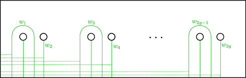
(a) The orientable case.

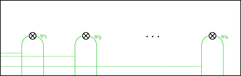
(b) The non-orientable case.

Figure 3.4: Another perspective on the basis elements depicted in Figures 2(c) and 2(d).

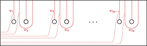
(a) The orientable case.

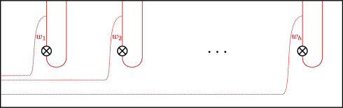
(b) The non-orientable case.

Figure 3.5: Another perspective on the basis elements depicted in Figures 3(c) and 3(d).

Notation 3.23

We denote by $\sigma_{1}\in\mathrm{MCG}(\mathscr{S}^{\natural n})$ the mapping class illustrated in Figure 3.6: it braids the left-most two handles if $\mathscr{S}=\mathbb{T}$ and it braids the left-most two crosscaps if $\mathscr{S}=\mathbb{M}$.

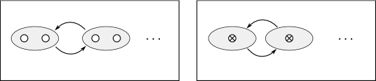
Figure 3.6: The braiding element $\sigma_{1}\in\mathrm{MCG}(S)$ when $S=\Sigma_{g,1}$ (left) and $S=\mathscr{N}_{h,1}$ (right).

Lemma 3.24

The following identities hold in $\mathfrak{L}^{\star}_{(\mathbf{k},\ell)}(\mathtt{n})$ for $\ell\geqslant 1$:

$$\sigma_{1}^{-1}\left(([\varnothing,\varnothing],[w_{3},w_{4}],\ldots)\right) =([w_{3},w_{4}],[\varnothing,\varnothing],\ldots)$$ (3.15)

$$\sigma_{1}^{-1}\left(([\varnothing],[w_{2}],\ldots)\right) =([w_{2}],[\varnothing],\ldots)$$ (3.16)

and in $\mathfrak{L}^{v}_{(\mathbf{k},\ell^{\prime})}(\mathtt{n})$ for $\ell^{\prime}\leqslant 2$ (recall that $\mathfrak{L}^{v}_{(\mathbf{k},\ell^{\prime})}=\mathfrak{L}^{u,v}_{(\mathbf{k},\ell^{\prime})}$ by Lemma 1.9):

$$\sigma_{1}\left(([\varnothing,\varnothing],[w_{3},w_{4}],\ldots)^{v}\right) =([w_{3},w_{4}],[\varnothing,\varnothing],\ldots)^{v}$$ (3.17)

$$\sigma_{1}\left(([\varnothing],[w_{2}],\ldots)^{v}\right) =([w_{2}],[\varnothing],\ldots)^{v}$$ (3.18)

Proof.

Equations (3.15) and (3.16) are clear from the diagrams, using the fact that the label(s) corresponding to the left-most handle or crosscap are empty.

On the other hand, we see from the diagrams that the left-hand side of equation (3.17) is equal to the element illustrated in Figure 7(a). This differs from the right-hand side of equation (3.17) only in the choice of tether. We therefore need to show that the difference between the two tethers, which is the based loop of configurations illustrated in Figure 7(b), projects to the trivial element of the group $Q_{(\mathbf{k},\ell^{\prime})}(\mathbb{T})$. This is obvious for $\ell^{\prime}=1$ since the group $Q_{(\mathbf{k},1)}(\mathbb{T})$ is always trivial. For $\ell^{\prime}=2$, we recall from Lemma 1.17 that $Q_{(\mathbf{k},2)}(\mathbb{T})$ is simply a product of copies of $\mathbb{Z}/2$, one for each block of the partition $\mathbf{k}=\boldsymbol{\{}k_{1};\ldots;k_{r}\boldsymbol{\}}$ with $k_{i}\geqslant 2$. The projection onto $Q_{(\mathbf{k},2)}(\mathbb{T})$ records the writhe (modulo $2$) of each block of strands (in a surface of positive genus the writhe is only well-defined modulo $2$). It is clear that the writhe of the loop of configurations illustrated in Figure 7(b) is trivial for each block. This establishes equation (3.17).

We argue similarly for equation (3.18). (Again, the case $\ell^{\prime}=1$ being obvious, we just consider $\ell^{\prime}=2$.) The left-hand side is equal to the element illustrated in Figure 8(a), which differs from the right-hand side only by its choice of tether; the difference between the two tethers forms the based loop of configurations illustrated in Figure 8(b). We therefore just have to show that this projects to the trivial element of the group $Q_{(\mathbf{k},2)}(\mathbb{M})$. This time the group $Q_{(\mathbf{k},2)}(\mathbb{M})$ is a product of $r^{\prime}+r$ copies of $\mathbb{Z}/2$, where $r^{\prime}$ denotes the number of blocks of the partition $\mathbf{k}$ with $k_{i}\geqslant 2$; see Lemma 1.17. The first $r^{\prime}$ copies of $\mathbb{Z}/2$, in the projection to $Q_{(\mathbf{k},2)}(\mathbb{M})$ of a loop of configurations, record the writhe of each block of strands; the remaining $r$ copies of $\mathbb{Z}/2$ record, for each block of strands, the number of times modulo $2$ that a strand from that block passes through a crosscap. As before, it is clear that the writhe of the loop of configurations illustrated in Figure 8(b) is trivial for each block; thus the first $r^{\prime}$ coordinates of its projection to $Q_{(\mathbf{k},2)}(\mathbb{M})$ are zero. Moreover, each strand in this loop of configurations passes around a crosscap an integer number of times, which corresponds to passing through a crosscap an even number of times; thus the last $r$ coordinates of its projection to $Q_{(\mathbf{k},2)}(\mathbb{M})$ are also zero. This establishes equation (3.18). ∎

Remark 3.25

Equations (3.15) and (3.16) of Lemma 3.24 hold for all $\ell\geqslant 1$. On the other hand, we used the explicit structure of the quotient group $Q_{(\mathbf{k},2)}(\mathscr{S})$ (and the fact that $Q_{(\mathbf{k},1)}(\mathscr{S})$ is trivial) to prove equations (3.17) and (3.18). For $\ell^{\prime}\geqslant 3$ the proof shows that these equations hold up to a unit scalar, which is the image in $Q_{(\mathbf{k},\ell^{\prime})}(\mathscr{S})$ of the loops in Figures 7(b) and 8(b) for $\mathscr{S}=\mathbb{T}$ and $\mathscr{S}=\mathbb{M}$ respectively. We do not know whether this scalar is trivial in these cases.

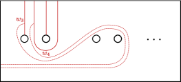
(a) The left-hand side of equation (3.17).

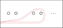
(b) A loop given by the difference of two tethers.

Figure 3.7: The left-hand side of equation (3.17) differs from the right-hand side of equation (3.17) by the scalar given by the image in $Q_{(\mathbf{k},2)}(\mathbb{T})$ of the loop illustrated on the right.

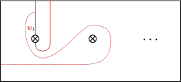
(a) The left-hand side of equation (3.18).

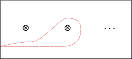
(b) A loop given by the difference of two tethers.

Figure 3.8: The left-hand side of equation (3.18) differs from the right-hand side of equation (3.18) by the scalar given by the image in $Q_{(\mathbf{k},2)}(\mathbb{M})$ of the loop illustrated on the right.

Remark 3.26

We will view equations (3.17) and (3.18) as being statements about the action of $(\sigma_{1}^{-1})^{\dagger}=\sigma_{1}$, where $(-)^{\dagger}$ is the operation that inverts the braiding of a braided monoidal category; see the beginning of §1.1.

3.3.2 Classical homological representation functors

We prove here Theorem B for the homological representation functors of mapping class groups in the classical (non-vertical) setting, i.e. the functors $\mathfrak{L}_{(\mathbf{k},\ell)}(\mathbf{\Gamma})$, $\mathfrak{L}^{u}_{(\mathbf{k},\ell)}(\mathbf{\Gamma})$, $\mathfrak{L}_{(\mathbf{k},\ell)}(\boldsymbol{\mathcal{N}})$ and $\mathfrak{L}^{u}_{(\mathbf{k},\ell)}(\boldsymbol{\mathcal{N}})$ defined in §1.3.3, for any $\mathbf{k}\vdash k\geqslant 1$ and $\ell\geqslant 1$. Following our notation so far in §3.3, we make all further reasoning, as much as possible, on the (generic) functor $\mathfrak{L}^{\star}_{(\mathbf{k},\ell)}$, which denotes any one of the functors (1.13) and (1.14).

The key technical result (Theorem 3.27) in this section states that the isomorphisms of modules (3.14) assemble into an isomorphism of functors on $\langle\mathcal{M},\mathcal{M}\rangle$. Moreover, we consider the embedding of $\mathbb{Z}[Q^{\star}_{(\mathbf{k},\ell)}(\mathscr{S})]$-modules $(\Delta^{\prime}_{\mathtt{1}}\mathfrak{L}^{\star}_{(\mathbf{k},\ell)})_{\mathtt{n}}\colon\delta_{\mathtt{1}}\mathfrak{L}^{\star}_{(\mathbf{k},\ell)}(\mathtt{n})\hookrightarrow\tau_{\mathtt{1}}\mathfrak{L}^{\star}_{(\mathbf{k},\ell)}(\mathtt{n})$ defined by sending each generating tuple $\mathbf{w}$ to itself. The second part of the statement of Theorem 3.27 is that these assemble into a functor that provides a splitting of the (short) exact sequence (3.1).

Theorem 3.27

For each partition $\mathbf{k}\vdash k\geqslant 1$, each integer $\ell\geqslant 1$ and $\star$ either the blank space or $\star=u$, the exact sequence (3.1) induces the following isomorphisms in the functor categories $\mathbf{Fct}(\langle\mathcal{M}_{2}^{+},\mathcal{M}_{2}^{+}\rangle,{\mathbb{Z}[Q^{\star}_{(\mathbf{k},\ell)}(\mathbb{T})]}{}\textrm{-}\mathrm{Mod}^{\bullet})$ and $\mathbf{Fct}(\langle\mathcal{M}_{2}^{-},\mathcal{M}_{2}^{-}\rangle,{\mathbb{Z}[Q^{\star}_{(\mathbf{k},\ell)}(\mathbb{M})]}{}\textrm{-}\mathrm{Mod}^{\bullet})$ respectively:

$$\begin{split}\tau_{\mathtt{1}}\mathfrak{L}^{\star}_{(\mathbf{k},\ell)}(\mathbf{\Gamma})&\cong\mathfrak{L}^{\star}_{(\mathbf{k},\ell)}(\mathbf{\Gamma})\mathbin{\textstyle\bigoplus}\left(\underset{\mathbf{k}^{\prime\prime}\in\{\mathbf{k}-2\}}{\bigoplus}\tau_{\mathtt{1}}\mathfrak{L}^{\star}_{(\mathbf{k}^{\prime\prime},\ell)}(\mathbf{\Gamma})\right)\\ &\phantom{\cong}\hskip 20.00003pt\mathbin{\textstyle\bigoplus}\left(\underset{1\leqslant j\leqslant r}{\bigoplus}\tau_{\mathtt{1}}\mathfrak{L}^{\star}_{(\mathbf{k}_{j},\ell)}(\mathbf{\Gamma})\right)\mathbin{\textstyle\bigoplus}\left(\underset{1\leqslant j\leqslant r}{\bigoplus}\tau_{\mathtt{1}}\mathfrak{L}^{\star}_{(\mathbf{k}_{j},\ell)}(\mathbf{\Gamma})\right),\end{split}$$ (3.19)

$$\begin{split}\tau_{\mathtt{1}}\mathfrak{L}^{\star}_{(\mathbf{k},\ell)}(\boldsymbol{\mathcal{N}})&\cong\mathfrak{L}^{\star}_{(\mathbf{k},\ell)}(\boldsymbol{\mathcal{N}})\mathbin{\textstyle\bigoplus}\left(\underset{1\leqslant j\leqslant r}{\bigoplus}\tau_{\mathtt{1}}\mathfrak{L}^{\star}_{(\mathbf{k}_{j},\ell)}(\boldsymbol{\mathcal{N}})\right).\end{split}$$ (3.20)

These isomorphisms also hold after any change of rings operation.

Proof.

The strategy consists in showing that the module isomorphisms $\{(\mathfrak{i}_{(\mathbf{k},\ell)})_{\mathtt{n}}=\eqref{eq:isom-of-modules_mcg}\}$ assemble into an isomorphism $\mathfrak{i}_{(\mathbf{k},\ell)}\colon\bigoplus_{\mathbf{k}^{\prime}}\tau_{\mathtt{1}}\mathfrak{L}^{\star}_{(\mathbf{k}^{\prime},\ell)}\overset{\sim}{\to}\delta_{\mathtt{1}}\mathfrak{L}^{\star}_{(\mathbf{k},\ell)}$ of functors on $\langle\mathcal{M},\mathcal{M}\rangle$, while the morphisms $\{(\Delta^{\prime}_{\mathtt{1}}\mathfrak{L}^{\star}_{(\mathbf{k},\ell)})_{\mathtt{n}}\}$ assemble into a natural transformation that is a section of $\Delta_{\mathtt{1}}\mathfrak{L}^{\star}_{(\mathbf{k},\ell)}$.

First, we prove the commutation of $(\mathfrak{i}_{(\mathbf{k},\ell)})_{\mathtt{n}}$ and $(\Delta^{\prime}_{\mathtt{1}}\mathfrak{L}^{\star}_{(\mathbf{k},\ell)})_{\mathtt{n}}$ with respect to the action of $\mathrm{MCG}(\mathscr{S}^{\natural n})$. For each element $\rho$ of $\mathrm{MCG}(\mathscr{S}^{\natural n})$ and $\mathbf{k}^{\prime}\in\{\mathbf{k}-j\}$ with $j\leqslant 2$, the morphisms $\tau_{\mathtt{1}}\mathfrak{L}^{\star}_{(\mathbf{k}^{\prime},\ell)}(\rho)$ and $\delta_{\mathtt{1}}\mathfrak{L}^{\star}_{(\mathbf{k},\ell)}(\rho)$ are induced by the action of $\mathrm{id}_{\mathtt{1}}\natural\rho$ on the Borel-Moore homology classes supported on the embedded graph $\mathbb{W}^{\mathscr{S}}_{1+n}\subset\mathscr{S}^{\natural(1+n)}$. It follows from a disjoint support argument (Lemma 3.22) that the action of the mapping class group $\mathrm{MCG}(\mathscr{S}^{\natural n})$ does not affect the first two (if $\mathscr{S}=\mathbb{T}$) or one (if $\mathscr{S}=\mathbb{M}$) entries of a tuple corresponding to a generator. We thus deduce that $(\mathfrak{i}_{(\mathbf{k},\ell)})_{\mathtt{n}}$ and $(\Delta^{\prime}_{\mathtt{1}}\mathfrak{L}^{\star}_{(\mathbf{k},\ell)})_{\mathtt{n}}$ commute with the action of $\rho$, since they only affect the first two or one entries of a tuple. Therefore, the morphisms $\{(\mathfrak{i}_{(\mathbf{k},\ell)})_{\mathtt{n}}\}_{\mathtt{n}\in\mathrm{Obj}(\mathcal{M})}$ and $\{(\Delta^{\prime}_{\mathtt{1}}\mathfrak{L}^{\star}_{(\mathbf{k},\ell)})_{\mathtt{n}}\}_{\mathtt{n}\in\mathrm{Obj}(\mathcal{M})}$ define natural transformations $\mathfrak{i}_{(\mathbf{k},\ell)}$ and $\Delta^{\prime}_{\mathtt{1}}\mathfrak{L}^{\star}_{(\mathbf{k},\ell)}$ in $\mathbf{Fct}(\mathcal{M},{\mathbb{Z}[Q^{\star}_{(\mathbf{k},\ell)}(\mathscr{S})]}{}\textrm{-}\mathrm{Mod}^{\bullet})$.

We now prove that $\mathfrak{i}_{(\mathbf{k},\ell)}$ and $\Delta^{\prime}_{\mathtt{1}}\mathfrak{L}^{\star}_{(\mathbf{k},\ell)}$ are actually natural transformations of functors on $\langle\mathcal{M},\mathcal{M}\rangle$ by using the approach of Lemma 1.2. We fix an integer $\mathtt{n}\geqslant\mathtt{1}$, the proof being trivial for $\mathtt{n}=\mathtt{0}$. We note from (1.1) that $\tau_{\mathtt{1}}\mathfrak{L}^{\star}_{(\mathbf{k},\ell)}([\mathtt{1},\mathrm{id}_{\mathtt{1}\natural\mathtt{n}}])=\mathfrak{L}^{\star}_{(\mathbf{k},\ell)}(\sigma_{1}^{-1})\circ\mathfrak{L}^{\star}_{(\mathbf{k},\ell)}([\mathtt{1},\mathrm{id}_{\mathtt{2}\natural\mathtt{n}}])$, where $\sigma_{1}\in\mathrm{Aut}_{\mathcal{M}}(S\natural S)$ is the element $b^{\mathcal{M}}_{\mathtt{1},\mathtt{1}}\natural\mathrm{id}_{\mathtt{n}}$ defined by the braiding $b^{\mathcal{M}}_{\mathtt{1},\mathtt{1}}\colon\mathtt{1}\natural\mathtt{1}\cong\mathtt{1}\natural\mathtt{1}$ (see Figure 3.6). We recall from the description of $\mathfrak{L}^{\star}_{(\mathbf{k},\ell)}([\mathtt{1},\mathrm{id}_{\mathtt{1}\natural\mathtt{n}}])$ in §3.3.1 that the morphism $\mathfrak{L}^{\star}_{(\mathbf{k},\ell)}([\mathtt{1},\mathrm{id}_{\mathtt{2}\natural\mathtt{n}}])$ is the map induced by the embedding of $\mathbb{W}^{S}_{1+n}$ into $\mathbb{W}^{S}_{2+n}$ given by sending the $i$th edge $(\mathbb{S}^{1}-\mathrm{pt})_{i}$ to the $(i+2)$nd edge $(\mathbb{S}^{1}-\mathrm{pt})_{i+2}$ (if $\mathscr{S}=\mathbb{T}$) or the $(i+1)$st edge $(\mathbb{S}^{1}-\mathrm{pt})_{i+1}$ (if $\mathscr{S}=\mathbb{M}$). In particular, in the image of $\mathfrak{L}^{\star}_{(\mathbf{k},\ell)}([\mathtt{1},\mathrm{id}_{\mathtt{2}\natural\mathtt{n}}])$, there are no configuration points on the two first edges $(\mathbb{S}^{1}-\mathrm{pt})_{1}$ and $(\mathbb{S}^{1}-\mathrm{pt})_{2}$ if $\mathscr{S}=\mathbb{T}$ or on the first edge $(\mathbb{S}^{1}-\mathrm{pt})_{1}$ if $\mathscr{S}=\mathbb{M}$. Then the morphism $\mathfrak{L}^{\star}_{(\mathbf{k},\ell)}(\sigma_{1}^{-1})$ corresponds to the action of $\sigma_{1}^{-1}$ on $\mathbb{W}^{S}_{2+n}$. It follows from equations (3.15) and (3.16) of Lemma 3.24 that for any generator $\mathbf{w}$ of $\bigoplus_{\mathbf{k}^{\prime}}\tau_{\mathtt{1}}\mathfrak{L}^{\star}_{(\mathbf{k}^{\prime},\ell)}(\mathtt{n})$, both $\delta_{\mathtt{1}}\mathfrak{L}^{\star}_{(\mathbf{k},\ell)}([\mathtt{1},\mathrm{id}_{\mathtt{1}\natural\mathtt{n}}])((\mathfrak{i}_{(\mathbf{k},\ell)})_{\mathtt{n}}(\mathbf{w}))$ and $(\mathfrak{i}_{(\mathbf{k},\ell)})_{\mathtt{1}+\mathtt{n}}(\bigoplus_{\mathbf{k}^{\prime}}\tau_{\mathtt{1}}\mathfrak{L}^{\star}_{(\mathbf{k}^{\prime},\ell)}([\mathtt{1},\mathrm{id}_{\mathtt{1}\natural\mathtt{n}}])(\mathbf{w}))$ are equal to:

$$\begin{cases}\sum_{1\leqslant j_{1}+j_{2}\leqslant r}([j_{1}w_{1},j_{2}w_{2}],[\varnothing,\varnothing],[w_{3},w_{4}],\ldots,[w_{2n+3},w_{2n+4}])&\textrm{if $S=\mathbb{T}$;}\\ \sum_{1\leqslant j\leqslant r}([jw_{1}],[\varnothing],[w_{2}],\ldots,[w_{n+2}])&\textrm{if $S=\mathbb{M}$.}\end{cases}$$

The same arguments using Lemma 3.24 also prove that $\tau_{\mathtt{1}}\mathfrak{L}^{\star}_{(\mathbf{k},\ell)}([\mathtt{1},\mathrm{id}_{\mathtt{1}\natural\mathtt{n}}])((\Delta^{\prime}_{\mathtt{1}}\mathfrak{L}^{\star}_{(\mathbf{k},\ell)})_{\mathtt{n}}(\mathbf{w}^{\prime}))$ and $(\Delta^{\prime}_{\mathtt{1}}\mathfrak{L}^{\star}_{(\mathbf{k},\ell)})_{\mathtt{1}+\mathtt{n}}(\delta_{\mathtt{1}}\mathfrak{L}^{\star}_{(\mathbf{k},\ell)}([\mathtt{1},\mathrm{id}_{\mathtt{1}\natural\mathtt{n}}])(\mathbf{w}^{\prime}))$ are both equal to:

$$\begin{cases}([w^{\prime}_{1},w^{\prime}_{2}],[\varnothing,\varnothing],[w^{\prime}_{3},w^{\prime}_{4}],\ldots,[w^{\prime}_{2n+3},w^{\prime}_{2n+4}])&\textrm{if $S=\mathbb{T}$;}\\ ([w^{\prime}_{1}],[\varnothing],[w^{\prime}_{2}],\ldots,[w^{\prime}_{n+2}])&\textrm{if $S=\mathbb{M}$;}\end{cases}$$

for any generator $\mathbf{w}^{\prime}$ of $\delta_{\mathtt{1}}\mathfrak{L}^{\star}_{(\mathbf{k},\ell)}(\mathtt{n})$. It then follows from the above equalities and induction on $\mathtt{m}\geqslant\mathtt{1}$ that the collections of morphisms $\{(\mathfrak{i}_{(\mathbf{k},\ell)})_{\mathtt{n}}\}_{\mathtt{n}\in\mathrm{Obj}(\mathcal{M})}$ and $\{(\Delta^{\prime}_{\mathtt{1}}\mathfrak{L}^{\star}_{(\mathbf{k},\ell)})_{\mathtt{n}}\}_{\mathtt{n}\in\mathrm{Obj}(\mathcal{M})}$ commute with the action of $[\mathtt{m},\mathrm{id}_{\mathtt{m}\natural\mathtt{n}}]$ for each $\mathtt{m}\geqslant\mathtt{1}$. Hence Relation (1.3) is satisfied for all $\mathtt{n}\in\mathrm{Obj}(\mathcal{M})$ and Lemma 1.2 implies that $\mathfrak{i}_{(\mathbf{k},\ell)}$ and $\Delta^{\prime}_{\mathtt{1}}\mathfrak{L}^{\star}_{(\mathbf{k},\ell)}$ are natural transformations of functors on $\langle\mathcal{M},\mathcal{M}\rangle$. In particular, it follows that $\mathfrak{i}_{(\mathbf{k},\ell)}$ is an isomorphism in $\mathbf{Fct}(\langle\mathcal{M},\mathcal{M}\rangle,{\mathbb{Z}[Q^{\star}_{(\mathbf{k},\ell)}(\mathscr{S})]}{}\textrm{-}\mathrm{Mod}^{\bullet})$ between the functors $\delta_{\mathtt{1}}\mathfrak{L}^{\star}_{(\mathbf{k},\ell)}$ and $\bigoplus_{\mathbf{k}^{\prime}}\tau_{\mathtt{1}}\mathfrak{L}^{\star}_{(\mathbf{k}^{\prime},\ell)}$.

It follows from the definitions that $(\Delta_{\mathtt{1}}\mathfrak{L}^{\star}_{(\mathbf{k},\ell)})_{\mathtt{n}}\circ(\Delta^{\prime}_{\mathtt{1}}\mathfrak{L}^{\star}_{(\mathbf{k},\ell)})_{\mathtt{n}}=\mathrm{id}_{\delta_{\mathtt{1}}\mathfrak{L}^{\star}_{(\mathbf{k},\ell)}(\mathtt{n})}$, and so $\Delta^{\prime}_{\mathtt{1}}\mathfrak{L}^{\star}_{(\mathbf{k},\ell)}$ is a section of $\Delta_{\mathtt{1}}\mathfrak{L}^{\star}_{(\mathbf{k},\ell)}$ in $\mathbf{Fct}(\langle\mathcal{M},\mathcal{M}\rangle,{\mathbb{Z}[Q^{\star}_{(\mathbf{k},\ell)}(\mathscr{S})]}{}\textrm{-}\mathrm{Mod}^{\bullet})$. Since $\kappa_{\mathtt{1}}\mathfrak{L}^{\star}_{(\mathbf{k},\ell)}=0$ (because $i_{\mathtt{1}}\mathfrak{L}^{\star}_{(\mathbf{k},\ell)}$ is clearly injective), we deduce that the exact sequence (3.1) is a split short exact sequence, which provides the isomorphisms (3.19) and (3.20).

Whenever we deal with a twisted homological representation functor, we note that the action on the ground ring $\mathbb{Z}[Q^{\star}_{(\mathbf{k},\ell)}(\mathscr{S})]$ does not affect any of the above reasoning, since $\mathfrak{L}^{\star}_{(\mathbf{k},\ell)}$ and $\bigoplus_{\mathbf{k}^{\prime}}\tau_{\mathtt{1}}\mathfrak{L}^{\star}_{(\mathbf{k}^{\prime},\ell)}$ are equipped with the same action as $\tau_{\mathtt{1}}\mathfrak{L}^{\star}_{(\mathbf{k},\ell)}$ via the change of rings operation of Convention 3.7; see Observation 3.6.

Finally, the fact that the isomorphisms (3.19) and (3.20) hold also after any change of rings operation follows from Lemma 3.8. ∎

3.3.3 Vertical-type alternatives

We now deal with the vertical-type alternatives of the homological representation functors for the mapping class groups of surfaces introduced in §1.3.3. Recalling that $\mathfrak{L}^{v}_{(\mathbf{k},\ell^{\prime})}=\mathfrak{L}^{u,v}_{(\mathbf{k},\ell^{\prime})}$ for $\ell^{\prime}\leqslant 2$ by Lemma 1.9, we just consider the functors $\mathfrak{L}^{v}_{(\mathbf{k},\ell^{\prime})}(\mathbf{\Gamma})$ for orientable surfaces and the functors $\mathfrak{L}^{v}_{(\mathbf{k},\ell^{\prime})}(\boldsymbol{\mathcal{N}})$ for non-orientable surfaces for $\ell^{\prime}\leqslant 2$. In particular, we do not consider the functors $\mathfrak{L}^{v}_{(\mathbf{k},\ell)}(\boldsymbol{\mathcal{N}})$ with $\ell\geqslant 3$ for non-orientable surfaces. This is because the proof of Theorem 3.28 below relies on the identities proven in Lemma 3.24 using the specific structure of the transformation groups $Q_{(\mathbf{k},2)}(\mathbb{T})$ and $Q_{(\mathbf{k},2)}(\mathbb{M})$ (see Lemma 1.17); on the other hand, the groups $Q_{(\mathbf{k},\ell)}(\mathbb{M})$ are not known for $\ell\geqslant 3$. We however conjecture that all of the following arguments, including the results of Theorem 3.28 and Theorem D, also hold for $\ell\geqslant 3$.

Theorem 3.28

For each partition $\mathbf{k}\vdash k\geqslant 1$, the exact sequence (3.1) induces the analogous isomorphisms to (3.19) and (3.20) for the functors $\mathfrak{L}^{v}_{(\mathbf{k},1)}(\mathbf{\Gamma})$, $\mathfrak{L}^{v}_{(\mathbf{k},2)}(\mathbf{\Gamma})$, $\mathfrak{L}^{v}_{(\mathbf{k},1)}(\boldsymbol{\mathcal{N}})$ and $\mathfrak{L}^{v}_{(\mathbf{k},2)}(\boldsymbol{\mathcal{N}})$. These results also hold after any change of rings operation.

Proof.

We fix $\ell^{\prime}\in\{1,2\}$. The analogous isomorphisms to (3.19) and (3.20) for the vertical-type alternatives follow mutatis mutandis from the proof of Theorem 3.27 by defining analogues $(\mathfrak{i}^{v}_{(\mathbf{k},\ell^{\prime})})_{\mathtt{n}}$ and $(\Delta^{\prime}_{\mathtt{1}}\mathfrak{L}^{v}_{(\mathbf{k},\ell^{\prime})})_{\mathtt{n}}$ to the morphisms $(\mathfrak{i}_{(\mathbf{k},\ell^{\prime})})_{\mathtt{n}}$ and $(\Delta^{\prime}_{\mathtt{1}}\mathfrak{L}_{(\mathbf{k},\ell^{\prime})})_{\mathtt{n}}$ for each $\mathtt{n}\in\mathrm{Obj}(\mathcal{M})$. The proof that these define natural transformations $\mathfrak{i}^{v}_{(\mathbf{k},\ell^{\prime})}$ and $\Delta^{\prime}_{\mathtt{1}}\mathfrak{L}^{v}_{(\mathbf{k},\ell^{\prime})}$ in $\mathbf{Fct}(\mathcal{M},{\mathbb{Z}[Q_{(\mathbf{k},\ell^{\prime})}]}{}\textrm{-}\mathrm{Mod})$ is a verbatim repetition of the first part of the proof of Theorem 3.27, again using Lemma 3.22. Then, the proof that $\mathfrak{i}^{v}_{(\mathbf{k},\ell^{\prime})}$ and $\Delta^{\prime}_{\mathtt{1}}\mathfrak{L}^{v}_{(\mathbf{k},\ell^{\prime})}$ are natural transformations in $\mathbf{Fct}(\langle\mathcal{M}^{\dagger},\mathcal{M}^{\dagger}\rangle,{\mathbb{Z}[Q_{(\mathbf{k},\ell^{\prime})}]}{}\textrm{-}\mathrm{Mod})$ is the same as the second part of the proof of Theorem 3.27, except that we now use equations (3.17) and (3.18) of Lemma 3.24 to understand the action of the braiding. ∎

Remark 3.29

We could define the functors $\mathfrak{L}^{v}_{(\mathbf{k},1)}(\mathbf{\Gamma})$, $\mathfrak{L}^{v}_{(\mathbf{k},2)}(\mathbf{\Gamma})$, $\mathfrak{L}^{v}_{(\mathbf{k},1)}(\boldsymbol{\mathcal{N}})$ and $\mathfrak{L}^{v}_{(\mathbf{k},2)}(\boldsymbol{\mathcal{N}})$ on the categories $\langle\mathcal{M}_{2}^{+},\mathcal{M}_{2}^{+}\rangle$ and $\langle\mathcal{M}_{2}^{-},\mathcal{M}_{2}^{-}\rangle$ respectively (i.e. without the opposite convention for the braiding of $\mathcal{M}_{2}$ induced by the ^† endofunctor; see §1.3.3). However, in this setting it is not clear that there are isomorphisms analogous to (3.19) and (3.20).

4 Polynomiality

In this section, we recollect the theory of polynomial functors in §4.1, then prove in §4.2–§4.3 the polynomiality results of Corollary C and Theorem D, and finally prove Corollary G in §4.4.

4.1 Notions of polynomiality

We review here the notions and basic properties of strong, very strong, split and weak polynomial functors. The first definitions of polynomial functors date back to Eilenberg and Mac Lane in [EM54] for functors on module categories. This notion has progressively been extended to deal with a more general framework, and has been the object of intensive study because of its applications in representation theory (see Djament, Touzé and Vespa [DTV19]), group cohomology (see Franjou, Friedlander, Scorichenko and Suslin [FFSS99]) and homological stability with twisted coefficients (see Randal-Williams and Wahl [RW17]). In particular, Djament and Vespa [DV19, §1] introduce the notions of strong and weak polynomial functors in the context of a functor category $\mathbf{Fct}(\mathcal{C},\mathcal{A})$, where $\mathcal{C}$ is a symmetric monoidal category where the unit is an initial object and $\mathcal{A}$ is a Grothendieck category. They are then extended to the case where $\mathcal{C}$ is pre-braided monoidal in [Sou19, Sou22], which also introduce the notion of very strong polynomial functor. See also [Pal17] for a comparison of the various instances of polynomial functors. All these notions extend verbatim to the present slightly larger framework from the previous literature on this topic (see [Sou22, §4] for instance), the various proofs being mutatis mutandis generalisations of these previous works. We also define the notion of split polynomial functor, a particular kind of very strong polynomial functor, following an analogous notion from [RW17].

For the remainder of §4.1, we fix a strict left-module $(\mathcal{M},\natural)$ over a strict monoidal small groupoid $(\mathcal{G},\natural,\mathtt{0})$ satisfying the same assumptions as in §3.1.1: $\mathcal{M}$ is a small (skeletal) groupoid, $(\mathcal{G},\natural,\mathtt{0})$ has no zero divisors, $\mathrm{Aut}_{\mathcal{G}}(\mathtt{0})=\{\mathrm{id}_{\mathtt{0}}\}$, $\mathcal{M}$ and $\mathcal{G}$ have the same set of objects identified with the non-negative integers $\mathbb{N}$, with the standard notation $\mathtt{n}$ to denote an object, and both the monoidal and module structures $\natural$ are given on objects by addition. We also consider a Grothendieck category $\mathcal{A}$: it would be enough to assume that $\mathcal{A}$ is abelian to define strong, very strong and split polynomiality, but we need $\mathcal{A}$ to be Grothendieck for the notion of weak polynomiality.

Strong, very strong and split polynomial functors.

The category of strong polynomial functors of degree less than or equal to $d\in\mathbb{N}$, denoted by $\mathcal{P}ol_{d}^{str}(\langle\mathcal{G},\mathcal{M}\rangle,\mathcal{A})$, is the full subcategory of $\mathbf{Fct}(\langle\mathcal{G},\mathcal{M}\rangle,\mathcal{A})$ defined by $\mathcal{P}ol_{d}^{str}(\langle\mathcal{G},\mathcal{M}\rangle,\mathcal{A})=\{0\}$ if $d<0$ and the objects of $\mathcal{P}ol_{d}^{str}(\langle\mathcal{G},\mathcal{M}\rangle,\mathcal{A})$ for $d\in\mathbb{N}$ are the functors $F$ such that the functor $\delta_{\mathtt{1}}(F)$ is an object of $\mathcal{P}ol_{d-1}^{str}(\langle\mathcal{G},\mathcal{M}\rangle,\mathcal{A})$. The smallest integer $d\in\mathbb{N}$ for which an object $F$ of $\mathbf{Fct}(\langle\mathcal{G},\mathcal{M}\rangle,\mathcal{A})$ is an object of $\mathcal{P}ol_{d}^{str}(\langle\mathcal{G},\mathcal{M}\rangle,\mathcal{A})$ is called the strong degree of $F$.

The category of very strong polynomial functors of degree less than or equal to $d\in\mathbb{N}$, denoted by $\mathcal{VP}ol_{d}(\langle\mathcal{G},\mathcal{M}\rangle,\mathcal{A})$, is the full subcategory of $\mathcal{P}ol_{d}^{str}(\langle\mathcal{G},\mathcal{M}\rangle,\mathcal{A})$ of the objects $F$ such that $\kappa_{\mathtt{1}}(F)=0$ and the functor $\delta_{\mathtt{1}}(F)$ is an object of $\mathcal{\mathcal{VP}}ol_{d-1}(\langle\mathcal{G},\mathcal{M}\rangle,\mathcal{A})$.

The category of split polynomial functors of degree less than or equal to $d\in\mathbb{N}$, denoted by $\mathcal{SP}ol_{d}(\langle\mathcal{G},\mathcal{M}\rangle,\mathcal{A})$, is the full subcategory of $\mathcal{VP}ol_{d}(\langle\mathcal{G},\mathcal{M}\rangle,\mathcal{A})$ of the objects $F$ such that the translation map $i_{\mathtt{1}}F\colon F\to\tau_{\mathtt{1}}F$ is split injective in $\mathbf{Fct}(\langle\mathcal{G},\mathcal{M}\rangle,\mathcal{A})$.

Weak polynomial functors.

Let $F$ be an object of $\mathbf{Fct}(\langle\mathcal{G},\mathcal{M}\rangle,\mathcal{A})$. We denote by $\kappa(F)$ the subfunctor $\sum_{\mathtt{n}\in\mathrm{Obj}(\mathcal{M})}\kappa_{\mathtt{n}}F$ of $F$. Let $K(\langle\mathcal{G},\mathcal{M}\rangle,\mathcal{A})$ be the full subcategory of $\mathbf{Fct}(\langle\mathcal{G},\mathcal{M}\rangle,\mathcal{A})$ of all those objects $F$ such that $\kappa(F)=F$. The category $K(\langle\mathcal{G},\mathcal{M}\rangle,\mathcal{A})$ is a thick subcategory of $\mathbf{Fct}(\langle\mathcal{G},\mathcal{M}\rangle,\mathcal{A})$ and it is closed under colimits; see [Sou22, Prop. 4.6]. Since the functor category $\mathbf{Fct}(\langle\mathcal{G},\mathcal{M}\rangle,\mathcal{A})$ is a Grothendieck category, the subcategory $K(\langle\mathcal{G},\mathcal{M}\rangle,\mathcal{A})$ is localising and we may define the quotient category of $\mathbf{Fct}(\langle\mathcal{G},\mathcal{M}\rangle,\mathcal{A})$ by $K(\langle\mathcal{G},\mathcal{M}\rangle,\mathcal{A})$; see [Gab62, Chapitre III]. We denote by $\mathbf{St}(\langle\mathcal{G},\mathcal{M}\rangle,\mathcal{A})$ this quotient category and by $\pi_{\langle\mathcal{G},\mathcal{M}\rangle}$ the associated quotient functor.

The translation functor $\tau_{\mathtt{1}}$ and the difference functor $\delta_{\mathtt{1}}$ in the category $\mathbf{Fct}(\langle\mathcal{G},\mathcal{M}\rangle,\mathcal{A})$ induce exact endofunctors of $\mathbf{St}(\langle\mathcal{G},\mathcal{M}\rangle,\mathcal{A})$ which commutes with colimits, respectively called again the translation functor $\tau_{\mathtt{1}}$ and the difference functor $\delta_{\mathtt{1}}$. In addition, we have the commutation relations $\delta_{\mathtt{1}}\circ\pi_{\langle\mathcal{G},\mathcal{M}\rangle}=\pi_{\langle\mathcal{G},\mathcal{M}\rangle}\circ\delta_{\mathtt{1}}$ and $\tau_{\mathtt{1}}\circ\pi_{\langle\mathcal{G},\mathcal{M}\rangle}=\pi_{\langle\mathcal{G},\mathcal{M}\rangle}\circ\tau_{\mathtt{1}}$. Therefore, the exact sequence (3.1) induces a short exact sequence $\mathit{Id}\hookrightarrow\tau_{\mathtt{1}}\twoheadrightarrow\delta_{\mathtt{1}}$ for the induced endofunctors of $\mathbf{St}(\langle\mathcal{G},\mathcal{M}\rangle,\mathcal{A})$. Finally, for another object $\mathtt{n}$ of $\mathcal{M}$, the endofunctors $\delta_{\mathtt{1}}$, $\delta_{\mathtt{n}}$, $\tau_{\mathtt{1}}$ and $\tau_{\mathtt{n}}$ of $\mathbf{St}(\langle\mathcal{G},\mathcal{M}\rangle,\mathcal{A})$ pairwise commute up to natural isomorphism.

We then define, inductively on $d\in\mathbb{N}$, the category of polynomial functors of degree less than or equal to $d$, denoted by $\mathcal{P}ol_{d}(\langle\mathcal{G},\mathcal{M}\rangle,\mathcal{A})$, to be the full subcategory of $\mathbf{St}(\langle\mathcal{G},\mathcal{M}\rangle,\mathcal{A})$ as follows. If $d<0$, $\mathcal{P}ol_{d}(\langle\mathcal{G},\mathcal{M}\rangle,\mathcal{A})=\{0\}$; if $d\geqslant 0$, the objects of $\mathcal{P}ol_{d}(\langle\mathcal{G},\mathcal{M}\rangle,\mathcal{A})$ are the functors $F$ such that the functor $\delta_{\mathtt{1}}(F)$ is an object of $\mathcal{P}ol_{d-1}(\langle\mathcal{G},\mathcal{M}\rangle,\mathcal{A})$. For an object $F$ of $\mathbf{St}(\langle\mathcal{G},\mathcal{M}\rangle,\mathcal{A})$ that is polynomial of degree less than or equal to $d\in\mathbb{N}$, the smallest integer $n\leqslant d$ for which $F$ is an object of $\mathcal{P}ol_{n}(\langle\mathcal{G},\mathcal{M}\rangle,\mathcal{A})$ is called the degree of $F$. An object $F$ of $\mathbf{Fct}(\langle\mathcal{G},\mathcal{M}\rangle,\mathcal{A})$ is weak polynomial of degree at most $d$ if its image $\pi_{\langle\mathcal{G},\mathcal{M}\rangle}(F)$ is an object of $\mathcal{P}ol_{d}(\langle\mathcal{G},\mathcal{M}\rangle,\mathcal{A})$. The degree of polynomiality of $\pi_{\langle\mathcal{G},\mathcal{M}\rangle}(F)$ is called the weak degree of $F$.

Remark 4.1

Since each object $\mathtt{n}$ is equal to $\mathtt{1}^{\natural n}$ in the category $\langle\mathcal{G},\mathcal{M}\rangle$, our definitions of the notions of strong, very strong, split and weak polynomiality are equivalent to the more classical ones with the analogous criteria on the functors $\tau_{\mathtt{n}}$, $\delta_{\mathtt{n}}$ and $\kappa_{\mathtt{n}}$ for all $\mathtt{n}\in\mathrm{Obj}(\mathcal{G})$ (instead of just $\mathtt{n}=\mathtt{1}$); see [DV19, Prop. 1.8], [Sou19, Prop. 3.9] and [Sou22, Prop. 4.4, (2)] for further details.

Finally, we recall useful properties of the categories associated with the different types of polynomial functors, which are proven in [Sou22, Props. 4.4, 4.10] (split polynomial functors are not considered there, but their study follows repeating mutatis mutandis this reference).

Proposition 4.2

Let $d\geqslant 0$ be an integer. The categories $\mathcal{P}ol_{d}^{str}(\langle\mathcal{G},\mathcal{M}\rangle,\mathcal{A})$, $\mathcal{VP}ol_{d}(\langle\mathcal{G},\mathcal{M}\rangle,\mathcal{A})$ and $\mathcal{SP}ol_{d}(\langle\mathcal{G},\mathcal{M}\rangle,\mathcal{A})$ are closed under the translation functor. The categories $\mathcal{P}ol_{d}^{str}(\langle\mathcal{G},\mathcal{M}\rangle,\mathcal{A})$ and $\mathcal{VP}ol_{d}(\langle\mathcal{G},\mathcal{M}\rangle,\mathcal{A})$ are closed under extensions. The category $\mathcal{P}ol_{d}^{str}(\langle\mathcal{G},\mathcal{M}\rangle,\mathcal{A})$ is closed under colimits. The categories $\mathcal{VP}ol_{d}(\langle\mathcal{G},\mathcal{M}\rangle,\mathcal{A})$ and $\mathcal{SP}ol_{d}(\langle\mathcal{G},\mathcal{M}\rangle,\mathcal{A})$ are closed under normal subobjects and under extensions. As a subcategory of $\mathbf{St}(\langle\mathcal{G},\mathcal{M}\rangle,\mathcal{A})$, the category $\mathcal{P}ol_{d}(\langle\mathcal{G},\mathcal{M}\rangle,\mathcal{A})$ is thick, complete and cocomplete.

4.2 For surface braid group functors

In this section, we prove the polynomiality properties of Corollary C and Theorem D for the homological representation functors for surface braid groups defined in §1.3.1 and §1.3.2. Throughout §4.2, we consider homological representation functors indexed by a partition $\mathbf{k}\vdash k$ of an integer $k\geqslant 1$ and by the stage $\ell\geqslant 1$ of a lower central series.

4.2.1 Classical homological representation functors

We prove here Corollary C in the classical (i.e. non-vertical) setting for homological representation functors. These polynomiality results actually hold both for the standard functors (i.e. $\mathfrak{LB}_{(\mathbf{k},\ell)}$ and $\mathfrak{L}_{(\mathbf{k},\ell)}(S)$) as well as for their untwisted versions (i.e. $\mathfrak{LB}^{u}_{(\mathbf{k},\ell)}$ and $\mathfrak{L}^{u}_{(\mathbf{k},\ell)}(S)$).

Proof of Corollary C for classical braid groups.

Following §3.2.2, we consider the functor $\mathfrak{LB}^{\star}_{(\mathbf{k},\ell)}$ where $\star$ either stands for the blank space or $\star=u$. Using the commutation property of the difference functor $\delta_{\mathtt{1}}$ with the translation functor $\tau_{\mathtt{1}}$, we deduce from Theorem 3.14 that, for all $0\leqslant m\leqslant k$, $\delta_{\mathtt{1}}^{m}\mathfrak{LB}^{\star}_{(\mathbf{k},\ell)}$ is a direct sum of functors of the form $\tau_{\mathtt{1}}^{m}\mathfrak{LB}^{\star}_{(\mathbf{k}^{\prime},\ell)}$ where $\mathbf{k}^{\prime}\in\{\mathbf{k}-k^{\prime}\}$ for $0\leqslant k^{\prime}\leqslant m$ (see Notation 3.2), while $\kappa_{\mathtt{1}}\mathfrak{LB}^{\star}_{(\mathbf{k},\ell)}=0$.

For $k=1$, we note that $\tau_{\mathtt{1}}\mathfrak{LB}^{\star}_{(0,\ell)}$ is the subobject of the constant functor at $\mathbb{Z}[Q_{((1),2)}(\mathbb{D})]$ with $\tau_{\mathtt{1}}\mathfrak{LB}^{\star}_{(0,\ell)}(\mathtt{0})=0$ and $\tau_{\mathtt{1}}\mathfrak{LB}^{\star}_{(0,\ell)}(\mathtt{n})=\mathbb{Z}[Q_{((1),2)}(\mathbb{D})]$ for $\mathtt{n}\geqslant\mathtt{1}$. Hence $\mathfrak{LB}^{\star}_{((1),\ell)}$ is weak polynomial of degree $1$ and $\delta_{\mathtt{1}}^{2}\mathfrak{LB}^{\star}_{((1),\ell)}$ is the functor whose unique non-null value is $\delta_{\mathtt{1}}^{2}\mathfrak{LB}^{\star}_{((1),\ell)}(\mathtt{0})=\mathbb{Z}[Q_{((1),2)}(\mathbb{D})]$. A fortiori $\mathfrak{LB}^{\star}_{((1),\ell)}$ is strong polynomial of degree $2$. For $k\geqslant 2$, we first note that for all integers $d\geqslant 2$, $\tau_{\mathtt{1}}^{2}\mathfrak{LB}^{\star}_{(0,\ell)}=\tau_{\mathtt{1}}^{d}\mathfrak{LB}^{\star}_{(0,\ell)}$ is a constant functor and thus it is both very strong and weak polynomial of degree $0$. Then, it follows from the above description of $\delta_{\mathtt{1}}^{m}(\mathfrak{LB}^{\star}_{(\mathbf{k},\ell)})$ by a clear induction on $k$ that $\mathfrak{LB}^{\star}_{(\mathbf{k},\ell)}$ is both strong and weak polynomial of degree $k$. Then, noting from Theorem 3.14 that $\kappa_{\mathtt{1}}(\mathfrak{LB}^{\star}_{(\mathbf{k},\ell)})=0$ and again viewing $\delta_{\mathtt{1}}^{m}(\mathfrak{LB}^{\star}_{(\mathbf{k},\ell)})$ as a direct sum of functors of the form $\tau_{\mathtt{1}}^{m}(\mathfrak{LB}^{\star}_{(\mathbf{k}^{\prime},\ell)})$, the commutation property of the evanescence functor $\kappa_{\mathtt{1}}$ and the translation functor $\tau_{\mathtt{1}}$ implies that $\kappa_{\mathtt{1}}(\delta_{\mathtt{1}}^{m}(\mathfrak{LB}^{\star}_{(\mathbf{k},\ell)}))=0$ for all integers $1\leqslant m\leqslant k$: this proves that $\mathfrak{LB}^{\star}_{(\mathbf{k},\ell)}$ is very strong polynomial of degree $k$. ∎

Proof of Corollary C for surface braid groups.

Following §3.2.3, we use here the notation $\mathfrak{L}^{\star}_{(\mathbf{k},\ell)}(S)$ where $\star$ either stands for the blank space or $\star=u$ and $S$ is either $\Sigma_{g,1}$ or $\mathscr{N}_{h,1}$ with $g,h\geqslant 1$. We proceed by induction on $k\geqslant 0$. We first note that the functor $\mathfrak{L}^{\star}_{(0,\ell)}(S)$ is very strong polynomial of degree $0$ since it is constant.

Now, for $k\geqslant 1$, we have by Theorem 3.19 that the difference functor $\delta_{\mathtt{1}}\mathfrak{L}^{\star}_{(\mathbf{k},\ell)\mid\geqslant 2}(S)$ is an extension of the atomic functor $\tau_{\mathtt{1}}\mathfrak{L}^{\star}_{(\mathbf{k},\ell)\mid\geqslant 2}(S)(\mathtt{1})$ by a direct sum of functors of the form $(\tau_{\mathtt{1}}\mathfrak{L}^{\star}_{(\mathbf{k}^{\prime},\ell)}(S))_{\mid\geqslant 2}$ where $\mathbf{k}^{\prime}\in\{\mathbf{k}-1\}$ (see Notation 3.2). We also recall that $\mathfrak{L}^{\star}_{(\mathbf{k},\ell)}(S)$ is an extension of the atomic functor $\mathfrak{L}^{\star}_{(\mathbf{k},\ell)}(S)(\mathtt{1})$ by $\mathfrak{L}^{\star}_{(\mathbf{k},\ell)\mid\geqslant 2}(S)$. Using the commutation property of the difference functor $\delta_{\mathtt{1}}$ and the translation functor $\tau_{\mathtt{1}}$, we see by the inductive assumption that each functor $\tau_{\mathtt{1}}\mathfrak{L}^{\star}_{(\mathbf{k}^{\prime},\ell)}(S)$ is strong and weak polynomial of degree $k-1$. Also, the atomic functor $\mathfrak{L}^{\star}_{(\mathbf{k},\ell)}(S)(\mathtt{1})$ is strong polynomial of degree $1$ while weak polynomial of degree $0$ by definition. We therefore deduce from Proposition 4.2 that the functors $\mathfrak{L}^{\star}_{(\mathbf{k},\ell)\mid\geqslant 2}(S)$ and $\mathfrak{L}^{\star}_{(\mathbf{k},\ell)}(S)$ are both strong and weak polynomial of degree at most $k$. Now, in the stable category $\mathbf{St}(\langle\boldsymbol{\beta},\boldsymbol{\beta}^{S}\rangle,{\mathbb{Z}[Q^{\star}_{(\mathbf{k},\ell)}(S)]}{}\textrm{-}\mathrm{Mod}^{\bullet})$, by Theorem 3.19 and the commutation properties of $\delta_{\mathtt{1}}$ with colimits and with $\pi_{\langle\boldsymbol{\beta},\boldsymbol{\beta}^{S}\rangle}$, the functor $\delta_{\mathtt{1}}^{k}\pi_{\langle\boldsymbol{\beta},\boldsymbol{\beta}^{S}\rangle}(\mathfrak{L}^{\star}_{(\mathbf{k},\ell)\mid\geqslant 2}(S))$ surjects onto each $\delta_{\mathtt{1}}^{k-1}\pi_{\langle\boldsymbol{\beta},\boldsymbol{\beta}^{S}\rangle}((\tau_{\mathtt{1}}\mathfrak{L}^{\star}_{(\mathbf{k}^{\prime},\ell)}(S))_{\mid\geqslant 2})$, which is non-null by the inductive assumption. Also, the image $\pi_{\langle\boldsymbol{\beta},\boldsymbol{\beta}^{S}\rangle}(\mathfrak{L}^{\star}_{(\mathbf{k},\ell)}(S)(\mathtt{1}))$ is null, so $\pi_{\langle\boldsymbol{\beta},\boldsymbol{\beta}^{S}\rangle}(\mathfrak{L}^{\star}_{(\mathbf{k},\ell)}(S))\cong\pi_{\langle\boldsymbol{\beta},\boldsymbol{\beta}^{S}\rangle}(\mathfrak{L}^{\star}_{(\mathbf{k},\ell)\mid\geqslant 2}(S))$. So, the weak degrees of $\mathfrak{L}^{\star}_{(\mathbf{k},\ell)\mid\geqslant 2}(S)$ and $\mathfrak{L}^{\star}_{(\mathbf{k},\ell)}(S)$ are both exactly $k$. Furthermore, the strong degree is always greater than or equal to the weak one: this is a direct consequence of the commutation property $\delta_{\mathtt{1}}\circ\pi_{\langle\boldsymbol{\beta},\boldsymbol{\beta}^{S}\rangle}=\pi_{\langle\boldsymbol{\beta},\boldsymbol{\beta}^{S}\rangle}\circ\delta_{\mathtt{1}}$. Hence, the strong degrees of $\mathfrak{L}^{\star}_{(\mathbf{k},\ell)\mid\geqslant 2}(S)$ and $\mathfrak{L}^{\star}_{(\mathbf{k},\ell)}(S)$ are also both exactly $k$.

The last property to be checked, in order to deduce very strong polynomiality, is that we have $\kappa_{\mathtt{1}}(\delta_{\mathtt{1}}^{m}(\mathfrak{L}^{\star}_{(\mathbf{k},\ell)}(S)))=0$ for all $0\leqslant m\leqslant k$. We have already checked the case of $m=0$, which follows from the evident injectivity of $i_{\mathtt{1}}\mathfrak{L}^{\star}_{(\mathbf{k},\ell)}(S)(\mathtt{n})$ for each $\mathtt{n}\in\mathrm{Obj}(\boldsymbol{\beta}^{S})$. We consider the long exact sequence (3.2) associated to the extension $\mathfrak{L}^{\star}_{(\mathbf{k},\ell)\mid\geqslant 2}(S)\hookrightarrow\mathfrak{L}^{\star}_{(\mathbf{k},\ell)}(S)\twoheadrightarrow\mathfrak{L}^{\star}_{(\mathbf{k},\ell)}(S)(\mathtt{1})$. We note that $\mathfrak{L}^{\star}_{(\mathbf{k},\ell)}(S)(\mathtt{1})=\kappa_{\mathtt{1}}(\mathfrak{L}^{\star}_{(\mathbf{k},\ell)}(S)(\mathtt{1}))$ while $\kappa_{\mathtt{1}}\mathfrak{L}^{\star}_{(\mathbf{k},\ell)}(S)=0$. Using Theorem 3.19, we deduce from the definition of the connecting map of the snake lemma that the cokernel of the injection $\mathfrak{L}^{\star}_{(\mathbf{k},\ell)}(S)(\mathtt{1})\hookrightarrow\delta_{\mathtt{1}}\mathfrak{L}^{\star}_{(\mathbf{k},\ell)\mid\geqslant 2}(S)$ induced by (3.2) is the (unique) extension of the atomic functor $\delta_{\mathtt{1}}\mathfrak{L}^{\star}_{(\mathbf{k},\ell)}(S)(\mathtt{1})$ (using the projection $\Delta_{\mathtt{1}}\mathfrak{L}^{\star}_{(\mathbf{k},\ell)}(S)(\mathtt{1})$) by the functor $\bigoplus_{1\leqslant j\leqslant r}(\tau_{\mathtt{1}}\mathfrak{L}^{\star}_{(\mathbf{k}_{j},\ell)}(S))_{\mid\geqslant 2}$ (similar to Definition 3.18 via Lemma 3.17). But this cokernel is also formally isomorphic to $(\delta_{\mathtt{1}}\mathfrak{L}^{\star}_{(\mathbf{k},\ell)}(S))_{\mid\geqslant 1}$. We thus obtain the short exact sequence $(\delta_{\mathtt{1}}\mathfrak{L}^{\star}_{(\mathbf{k},\ell)}(S))_{\mid\geqslant 1}\hookrightarrow\delta_{\mathtt{1}}\mathfrak{L}^{\star}_{(\mathbf{k},\ell)}(S)\twoheadrightarrow\delta_{\mathtt{1}}(\mathfrak{L}^{\star}_{(\mathbf{k},\ell)}(S)(\mathtt{1}))$ with the explicit description of $(\delta_{\mathtt{1}}\mathfrak{L}^{\star}_{(\mathbf{k},\ell)}(S))_{\mid\geqslant 1}$ as an extension, and we consider its associated long exact sequence (3.2). Since we have $\delta_{\mathtt{1}}^{2}(\mathfrak{L}^{\star}_{(\mathbf{k},\ell)}(S)(\mathtt{1}))=\kappa_{\mathtt{1}}((\delta_{\mathtt{1}}\mathfrak{L}^{\star}_{(\mathbf{k},\ell)}(S))_{\mid\geqslant 1})=0$ as a direct consequence of the definitions and of the inductive assumption, we have an exact sequence $\kappa_{\mathtt{1}}\delta_{\mathtt{1}}\mathfrak{L}^{\star}_{(\mathbf{k},\ell)}(S)\hookrightarrow\delta_{\mathtt{1}}(\mathfrak{L}^{\star}_{(\mathbf{k},\ell)}(S)(\mathtt{1}))\to\delta_{\mathtt{1}}((\delta_{\mathtt{1}}\mathfrak{L}^{\star}_{(\mathbf{k},\ell)}(S))_{\mid\geqslant 1})\twoheadrightarrow\delta_{\mathtt{1}}^{2}\mathfrak{L}^{\star}_{(\mathbf{k},\ell)}(S)$. Once again, using Theorem 3.19 and the above description of $(\delta_{\mathtt{1}}\mathfrak{L}^{\star}_{(\mathbf{k},\ell)}(S))_{\mid\geqslant 1}$, it is routine to check that its middle morphism is an injection induced by the map $i_{\mathtt{1}}(\delta_{\mathtt{1}}\mathfrak{L}^{\star}_{(\mathbf{k},\ell)}(S))(\mathtt{0})$. Therefore, we have $\kappa_{\mathtt{1}}\delta_{\mathtt{1}}\mathfrak{L}^{\star}_{(\mathbf{k},\ell)}(S)=0$, i.e. the desired result for $m=1$.

Finally, we consider the long exact sequence (3.2) associated to the short exact sequence $\delta_{\mathtt{1}}(\mathfrak{L}^{\star}_{(\mathbf{k},\ell)}(S)(\mathtt{1}))\hookrightarrow\delta_{\mathtt{1}}((\delta_{\mathtt{1}}\mathfrak{L}^{\star}_{(\mathbf{k},\ell)}(S))_{\mid\geqslant 1})\twoheadrightarrow\delta_{\mathtt{1}}^{2}\mathfrak{L}^{\star}_{(\mathbf{k},\ell)}(S)$. Since we have $\delta_{\mathtt{1}}^{2}(\mathfrak{L}^{\star}_{(\mathbf{k},\ell)}(S)(\mathtt{1}))=0$ and $\kappa_{\mathtt{1}}(\delta_{\mathtt{1}}^{2}\mathfrak{L}^{\star}_{(\mathbf{k},\ell)\mid\geqslant 1}(S))\cong\delta_{\mathtt{1}}(\mathfrak{L}^{\star}_{(\mathbf{k},\ell)}(S)(\mathtt{1}))$, we deduce that $\kappa_{\mathtt{1}}(\delta_{\mathtt{1}}^{2}\mathfrak{L}^{\star}_{(\mathbf{k},\ell)}(S))=0$, i.e. the desired result for $m=2$. Also, by the commutation property of $\delta_{\mathtt{1}}$ with $\tau_{\mathtt{1}}$ and with colimits, it then follows from the above description of $(\delta_{\mathtt{1}}\mathfrak{L}^{\star}_{(\mathbf{k},\ell)}(S))_{\mid\geqslant 1}$ as an extension and from Theorem 3.19 that $\delta_{\mathtt{1}}^{3}\mathfrak{L}^{\star}_{(\mathbf{k},\ell)}(S)\cong\bigoplus_{1\leqslant j\leqslant j^{\prime}\leqslant r}\tau_{\mathtt{1}}^{2}\delta_{\mathtt{1}}\mathfrak{L}^{\star}_{(\mathbf{k}_{j,j^{\prime}},\ell)\mid\geqslant 2}(S)$ (recall Notation 3.2 for the definition of $\mathbf{k}_{j,j^{\prime}}$). Then, by the inductive assumption, each $\tau_{\mathtt{1}}^{2}\delta_{\mathtt{1}}\mathfrak{L}^{\star}_{(\mathbf{k}_{j,j^{\prime}},\ell)\mid\geqslant 2}(S)$ is a very strong polynomial functor of degree $k-3$ and we deduce that $\kappa_{\mathtt{1}}(\delta_{\mathtt{1}}^{m}(\mathfrak{L}^{\star}_{(\mathbf{k},\ell)}(S)))=0$ for all $3\leqslant m\leqslant k$, which ends the proof. ∎

Remark 4.3

All of the above polynomiality results still hold after any non-zero change of rings operation: indeed, Theorems 3.14 and 3.19 also hold after such an operation and then the arguments of the proofs repeat mutatis mutandis.

In particular, the functors $\mathfrak{LB}_{((1),2)}\otimes\mathbb{C}[\mathbb{Z}]$ and $\mathfrak{LB}_{((2),2)}\otimes\mathbb{C}[\mathbb{Z}^{2}]$ correspond to the reduced Burau functor $\overline{\mathfrak{Bur}}$ and the Lawrence-Krammer functor $\mathfrak{LK}$ defined in [Sou19, §1.2]. The polynomiality results of Corollary C recover those of [Sou19, Props. 3.25 and 3.33] for the functors $\mathfrak{LB}_{((1),2)}\otimes\mathbb{C}[\mathbb{Z}]$ and $\mathfrak{LB}_{((2),2)}\otimes\mathbb{C}[\mathbb{Z}^{2}]$. Also, the corresponding key short exact sequences using [Sou19, §1.2] (i.e. (3.9) for $\mathbf{k}\in\{1,2\}$ and $\ell=2$) are proven via an alternative method, which is more algebraic than that of Theorem 3.14.

4.2.2 Vertical-type alternatives

We now deal with the vertical-type alternatives of the homological representation functors of the surface braid groups. Following the framework of §3.2, we consider the generic vertical homological representation functor $\mathfrak{L}^{\star,v}_{(\mathbf{k},\ell)}(S)$ where $\star$ either stands for the blank space or $\star=u$, $S\in\{\mathbb{D},\Sigma_{g,1},\mathscr{N}_{h,1}\}$ with $g\geqslant 1$ and $h\geqslant 1$ and the associated transformation group is denoted by $Q^{\star}_{(\mathbf{k},\ell)}(S)$. We recall from Proposition 2.6 that, for each $\mathtt{n}\in\mathrm{Obj}(\boldsymbol{\beta}^{S})$, the $\mathbb{Z}[Q^{\star}_{(\mathbf{k},\ell)}(S)]$-module $\mathfrak{L}^{\star,v}_{(\mathbf{k},\ell)}(S)(\mathtt{n})$ is free with basis indexed by the set of (“vertical”) tuples $\mathbf{w}^{v}$ as pictured in Figures 3(a) and 3(b), which has the same dimension as the (“classical”) functor $\mathfrak{L}^{\star}_{(\mathbf{k},\ell)}(S)(\mathtt{n})$.

First of all, we focus on a significant fact about the behaviour of the functor $\mathfrak{L}^{\star,v}_{(\mathbf{k},\ell)}(S)$ after applying the operation $\delta_{\mathtt{1}}$.

Lemma 4.4

The functor $\delta_{\mathtt{1}}\mathfrak{L}^{\star,v}_{(\mathbf{k},\ell)}(S)$ sends every morphism that is not an endomorphism to zero.

Proof.

Recall that, by construction (see Lemma 1.7), the morphism $\mathtt{n}\to\mathtt{1}\natural\mathtt{n}$ of the domain category $\langle\boldsymbol{\beta},\boldsymbol{\beta}^{S}\rangle$ is sent, under each of our functors $\mathfrak{L}^{\star,v}_{(\mathbf{k},\ell)}(S)$, to the map on Borel-Moore homology induced by the evident inclusion of configuration spaces. Since every morphism of the domain category that is not an endomorphism factors through one of these canonical morphisms, it suffices to show that all of these are sent to zero under $\delta_{\mathtt{1}}\mathfrak{L}^{\star,v}_{(\mathbf{k},\ell)}(S)$. In other words, we wish to show that the map labelled by $(*)$ in the following diagram is zero, where the rows are exact:

(4.1)

To do this, it suffices to show that there is a diagonal morphism making the two triangles commute. Recalling that $\tau_{\mathtt{1}}F(\mathtt{n})=F(\mathtt{1}\natural\mathtt{n})$ in general, we will be able to take the diagonal morphism to be the identity as long as the two maps labelled $(\dagger)$ and $(\ddagger)$ are equal (the top horizontal and left vertical maps in that square are always equal by definition of the natural transformation $\mathit{Id}\to\tau_{\mathtt{1}}$).

By definition of $\tau_{\mathtt{1}}\mathfrak{L}^{\star,v}_{(\mathbf{k},\ell)}(S)$, its action on the canonical morphism $\mathtt{n}\to\mathtt{1}\natural\mathtt{n}$ is given by the action of $\mathfrak{L}^{\star,v}_{(\mathbf{k},\ell)}(S)$ on the canonical morphism $\mathtt{1}\natural\mathtt{n}\to\mathtt{2}\natural\mathtt{n}$ composed with $(b_{\mathtt{1},\mathtt{1}}^{\boldsymbol{\beta}})^{-1}\natural\mathrm{id}_{\mathtt{n}}$, where $b_{\mathtt{1},\mathtt{1}}^{\boldsymbol{\beta}}$ is the braiding $\mathtt{1}\natural\mathtt{1}\cong\mathtt{1}\natural\mathtt{1}$ of the groupoid $\boldsymbol{\beta}$. This describes the map $(\dagger)$; on the other hand, the map $(\ddagger)$ is given simply by the action of $\mathfrak{L}^{\star,v}_{(\mathbf{k},\ell)}(S)$ on the canonical morphism $\mathtt{1}\natural\mathtt{n}\to\mathtt{2}\natural\mathtt{n}$. It is therefore enough to prove that the automorphism $b_{\mathtt{1},\mathtt{1}}^{\boldsymbol{\beta}}\natural\mathrm{id}_{\mathtt{n}}$, which canonically identifies with the Artin generator $\sigma_{1}$, acts by the identity on the image of $(\ddagger)$. This is immediate from Figure 4.1, where the image of an arbitrary basis element under $(\ddagger)$ is depicted in green (supported on the vertical arcs) and the support of a diffeomorphism representing the mapping class $\sigma_{1}$ is shaded in grey. Since these supports are disjoint, the action of $b_{\mathtt{1},\mathtt{1}}^{\boldsymbol{\beta}}\natural\mathrm{id}_{\mathtt{n}}$ on the image of $(\ddagger)$ is trivial. ∎

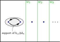
Figure 4.1: The support of a diffeomorphism representing the mapping class $\sigma_{1}=b_{\mathtt{1},\mathtt{1}}^{\boldsymbol{\beta}}\natural\mathrm{id}_{\mathtt{n}}$ and the image of an arbitrary basis element under the map $(\ddagger)$ of (4.1).

Remark 4.5

It is instructive to consider why the same argument does not also show that the functor $\delta_{\mathtt{1}}\mathfrak{L}^{\star}_{(\mathbf{k},\ell)}(S)$ sends every canonical morphism $\mathtt{n}\to\mathtt{1}\natural\mathtt{n}$ to the zero morphism. This boils down to the fact that, in the analogue of Figure 4.1 for the non-vertical version $\mathfrak{L}^{\star}_{(\mathbf{k},\ell)}(S)$ of the functor, the supports are not disjoint.

We are now ready prove the (non-)polynomiality results of Theorem D, which actually hold for any one of these vertical-type alternatives $\mathfrak{L}^{\star,v}_{(\mathbf{k},\ell)}(S)$ (i.e. also for the untwisted versions). In particular, this shows that these vertical-type alternatives exhibit unexpected interesting behaviour with respect to polynomiality, which thoroughly differs from their “classical” (non-vertical) counterparts studied in §3.2.2–§3.2.3. Indeed, they are not strong polynomial, which is a counterintuitive property since the dimensions of the representations encoded by each $\mathfrak{L}^{\star,v}_{(\mathbf{k},\ell)}(S)$ grow in the same polynomial way as those of $\mathfrak{L}^{\star}_{(\mathbf{k},\ell)}(S)$.

Proof of Theorem D for surface braid groups.

By similar reasoning to that of §3.2.1, we see that the map $\mathfrak{L}^{\star,v}_{(\mathbf{k},\ell)}(S)([\mathtt{1},\mathrm{id}_{\mathtt{1}\natural\mathtt{n}}])$ is the injection defined on basis elements by $(w_{1},\ldots,w_{g_{S}+n-1})^{v}\mapsto(\varnothing,w_{1},\ldots,w_{g_{S}+n-1})^{v}$, so it follows that $\delta_{\mathtt{1}}\mathfrak{L}^{\star,v}_{(\mathbf{k},\ell)}(S)(\mathtt{n})$ is a non-trivial free $\mathbb{Z}[Q^{\star}_{(\mathbf{k},\ell)}(\mathbb{D})]$-module with the same dimension as $\delta_{\mathtt{1}}\mathfrak{L}^{\star}_{(\mathbf{k},\ell)}(S)(\mathtt{n})$ for all $\mathtt{n}\geqslant\mathtt{1}$. Meanwhile it follows from Lemma 4.4 that $\delta_{\mathtt{1}}\mathfrak{L}^{\star,v}_{(\mathbf{k},\ell)}(S)$ assigns the trivial map to all morphisms of $\langle\boldsymbol{\beta},\boldsymbol{\beta}^{S}\rangle(\mathtt{n},\mathtt{m})$ with $\mathtt{n}\neq\mathtt{m}$. So $\delta_{\mathtt{1}}\mathfrak{L}^{\star,v}_{(\mathbf{k},\ell)}(S)$ is isomorphic to a direct sum of infinitely many atomic functors. It follows that $\delta_{\mathtt{1}}^{m}\mathfrak{L}^{\star,v}_{(\mathbf{k},\ell)}(S)\neq 0$ for any $m\in\mathbb{N}$ while $\pi_{\langle\boldsymbol{\beta},\boldsymbol{\beta}^{S}\rangle}(\delta_{\mathtt{1}}\mathfrak{L}^{\star,v}_{(\mathbf{k},\ell)}(S))=0$ in the stable category $\mathbf{St}(\langle\boldsymbol{\beta},\boldsymbol{\beta}^{S}\rangle,{\mathbb{Z}[Q^{\star}_{(\mathbf{k},\ell)}(\mathbb{D})]}{}\textrm{-}\mathrm{Mod}^{\bullet})$, whence the result. ∎

Remark 4.6

All of these non-polynomiality results still hold after any non-zero change of rings operation on the functors, since none of the steps of the proof are affected by such an operation.

Furthermore, the first steps of the proofs of Theorems 3.14 and 3.19 do go through in the vertical setting, inducing a short exact sequence of functors defined on the groupoid $\boldsymbol{\beta}^{S}$ for each $\mathfrak{L}^{\star,v}_{(\mathbf{k},\ell)}(S)$, analogous to (3.9), (3.10) and (3.13) but only at the level of automorphism groups.

Finally, we briefly deal with the duals of the homological representations of Theorems 3.14 and 3.19. Let us consider any one of the above homological representation functors $\mathfrak{L}^{\star}_{(\mathbf{k},\ell)}(S)$. By Corollary 2.9, the $\mathbf{B}_{n}(S)$-representation $H_{k}^{\partial}(C_{\mathbf{k}}(\mathbb{D}_{n}\natural S);\mathbb{Z}[Q^{\star}_{(\mathbf{k},\ell)}(S)]\otimes\mathcal{O})$ of §2.3 is the dual representation of $\mathfrak{L}^{\star}_{(\mathbf{k},\ell)}(S)(\mathtt{n})$. Gathering these representations and assigning for each $[\mathtt{m},\mathrm{id}_{\mathtt{m}\natural\mathtt{n}}]\in\langle\boldsymbol{\beta},\boldsymbol{\beta}^{S}\rangle$ the evident analogue of the map $\iota_{\mathtt{m},\mathtt{n}}$ of §1.2.4 for homology relative to the boundary, one may easily prove the analogue of Lemma 1.7 so that we define a functor $\mathfrak{L}^{\star,\vee}_{(\mathbf{k},\ell)}(S)\colon\langle\boldsymbol{\beta},\boldsymbol{\beta}^{S}\rangle\to(\mathbb{Z}[Q^{\star}_{(\mathbf{k},\ell)}(S)]\otimes\mathcal{O}){}\textrm{-}\mathrm{Mod}^{\bullet}$. Then the reasoning of the proof of Theorem D repeats verbatim:

Theorem 4.7

The functor $\mathfrak{L}^{\star,\vee}_{(\mathbf{k},\ell)}(S)$ is not strong polynomial, but is weak polynomial of degree $0$.

4.3 For mapping class group functors

In this section, we prove the polynomiality results of Corollary C and Theorem D for the homological representation functors for mapping class groups defined in §1.3.3. Following §3.3, we use the generic notation $\mathfrak{L}^{\star}_{(\mathbf{k},\ell)}$ for any one of the functors (1.13) and (1.14) indexed by a partition $\mathbf{k}\vdash k$ of an integer $k\geqslant 1$ and by the stage $\ell\geqslant 1$ of a lower central series, $\mathfrak{L}^{\star,v}_{(\mathbf{k},\ell)}$ for the vertical-type alternative functor, $Q^{\star}_{(\mathbf{k},\ell)}(\mathscr{S})$ with $\mathscr{S}\in\{\mathbb{T},\mathbb{M}\}$ for the associated transformation group and $\mathcal{M}$ for either $\mathcal{M}_{2}^{+}$ or $\mathcal{M}_{2}^{-}$.

Proof of Corollary C and Theorem D for mapping class groups.

Let $0\leqslant m\leqslant k$. Since $\delta_{\mathtt{1}}$ and $\tau_{\mathtt{1}}$ commute, we deduce from Theorem 3.27 by induction on $m$ that $\delta_{\mathtt{1}}^{m}\mathfrak{L}^{\star}_{(\mathbf{k},\ell)}$ is isomorphic to a direct sum of functors of the form $\tau_{\mathtt{1}}^{m}\mathfrak{L}^{\star}_{(\mathbf{k}^{\prime},\ell)}$ with $\mathbf{k}^{\prime}\in\bigcup_{i=m}^{2m}\{\mathbf{k}-i\}$ in the orientable setting and with $\mathbf{k}^{\prime}\in\{\mathbf{k}-m\}$ in the non-orientable setting (see Notation 3.2). In particular, $\delta_{\mathtt{1}}\mathfrak{L}^{\star}_{((1),\ell)}$ is isomorphic to the constant functor at $\mathbb{Z}[Q^{\star}_{((1),\ell)}(\mathscr{S})]$. Hence $\mathfrak{L}^{\star}_{((1),\ell)}$ is both split and weak polynomial of degree $1$. By the above direct sum decomposition of $\delta_{\mathtt{1}}^{m}\mathfrak{L}^{\star}_{(\mathbf{k},\ell)}$ and the fact that $\kappa_{\mathtt{1}}\mathfrak{L}^{\star}_{(\mathbf{k},\ell)}=0$, along with the fact that $\kappa_{\mathtt{1}}$ and $\tau_{\mathtt{1}}$ commute, it follows by induction on $k$ that $\mathfrak{L}^{\star}_{(\mathbf{k},\ell)}$ is both split and weak polynomial of degree $k$.

Fixing $\ell\in\{1,2\}$, the same polynomiality results follow for $\mathfrak{L}^{\star,v}_{(\mathbf{k},\ell)}$ by the same arguments, using Theorem 3.28 instead of Theorem 3.27. ∎

Remark 4.8

All of the polynomiality results for mapping class groups in Corollary C and Theorem D hold also after any non-zero change of rings operation on the functors, since none of the steps of the above proof are affected by such an operation.

We finish this section by briefly dealing with the duals of the homological representations of Theorem 3.27. By Corollary 2.9, the $\mathrm{MCG}(\mathscr{S}^{\natural n})$-representation $H_{k}^{\partial}(C_{\mathbf{k}}(\mathscr{S}^{\natural n}\smallsetminus I^{\prime});\mathbb{Z}[Q^{\star}_{(\mathbf{k},\ell)}(\mathscr{S})]\otimes\mathcal{O})$ of §2.3, for $\mathscr{S}\in\{\mathbb{T},\mathbb{M}\}$, is the dual of the $\mathrm{MCG}(\mathscr{S}^{\natural n})$-representation $H_{k}^{\mathrm{BM}}(C_{\mathbf{k}}(\mathscr{S}^{\natural n}\smallsetminus I^{\prime});\mathbb{Z}[Q^{\star}_{(\mathbf{k},\ell)}(\mathscr{S})])$. Assigning for each morphism $[\mathtt{m},\mathrm{id}_{\mathtt{m}\natural\mathtt{n}}]$ the obvious analogue of the map $\iota_{\mathtt{m},\mathtt{n}}$ of §1.2.4 for homology relative to the boundary, these collections of representations extend to functors $\mathfrak{L}^{\star,\vee}_{(\mathbf{k},\ell)}(\mathbf{\Gamma})$ and $\mathfrak{L}^{\star,\vee}_{(\mathbf{k},\ell)}(\boldsymbol{\mathcal{N}})$ of the form $\langle\mathcal{M}^{\dagger},\mathcal{M}^{\dagger}\rangle\to(\mathbb{Z}[Q^{\star}_{(\mathbf{k},\ell)}(\mathscr{S})]\otimes\mathcal{O}){}\textrm{-}\mathrm{Mod}$. We may then deduce analogous short exact sequences to those of Theorem 3.28, and Theorem D repeats verbatim for these functors:

Theorem 4.9

For $\ell\in\{1,2\}$, the functors $\mathfrak{L}^{\star,\vee}_{(\mathbf{k},\ell)}(\mathbf{\Gamma})$ and $\mathfrak{L}^{\star,\vee}_{(\mathbf{k},\ell)}(\boldsymbol{\mathcal{N}})$ are split polynomial and weak polynomial of degree $k$.

4.4 Analyticity of a quantum representation

Jackson and Kerler [JK11] introduce a representation $\mathbb{V}$ over the group ring $\mathbb{L}:=\mathbb{Z}[\mathfrak{s}^{\pm 1},\mathfrak{q}^{\pm 1}]$, called the generic Verma module, of $\mathbb{U}_{q}(\mathfrak{sl}_{2})$, the quantum enveloping algebra of the Lie algebra $\mathfrak{sl}_{2}$. Since $\mathbb{U}_{q}(\mathfrak{sl}_{2})$ is a quasitriangular Hopf algebra, the representation $\mathbb{V}$ comes equipped with an automorphism $S\in\mathrm{Aut}_{\mathbb{L}}(\mathbb{V}\otimes\mathbb{V})$. This induces a $\mathbf{B}_{n}$-representation on $\mathbb{V}^{\otimes n}$ given by sending $\sigma_{i}\in\mathbf{B}_{n}$ to $\mathrm{id}_{i-1}\otimes S\otimes\mathrm{id}_{n-i-1}$, which we call the Verma module representation; see [JK11, §1]. For $k\geqslant 1$, the weight space $V_{n,k}\subseteq\mathbb{V}^{\otimes n}$ is the eigenspace of the action of a certain generator $K\in\mathbb{U}_{q}(\mathfrak{sl}_{2})$ corresponding to the eigenvalue $\mathfrak{s}^{n}\mathfrak{q}^{-2k}$ and the highest weight space $W_{n,k}$ is its intersection with the kernel of the action of another generator $E\in\mathbb{U}_{q}(\mathfrak{sl}_{2})$. The $\mathbf{B}_{n}$-action on $\mathbb{V}^{\otimes n}$ restricts to sub-$\mathbf{B}_{n}$-representations on $V_{n,k}$ and $W_{n,k}$ for each $k\geqslant 1$. The first one is the quantum representation of $\mathbf{B}_{n}$ of weight $k$, while the second one is the quantum representation of $\mathbf{B}_{n}$ of highest weight $k$. The relation between the variables $\mathfrak{s}$ and $\mathfrak{q}$ and the generators $q$ and $t$ of $Q_{((2),2)}(\mathbb{D})=\mathbb{Z}^{2}=\mathbb{Z}\langle q,t\rangle$ (defining the representation $\mathfrak{LB}_{((2),2)}(\mathtt{n})$) is given by the ring homomorphism $\theta\colon\mathbb{K}:=\mathbb{Z}[q^{\pm 1},t^{\pm 1}]\to\mathbb{L}$ defined by $(q,t)\mapsto(\mathfrak{s}^{2},-\mathfrak{q}^{-2})$. (We note as a warning to the reader that the notation in the literature is not consistent; in particular [JK11] and [Mar22] use different notation from each other and from the notation used in this section, which is instead consistent with the notation of [Big01, Big02].) In particular, $\mathbb{L}$ is a left $\mathbb{K}$-module via $\theta$; the change of rings operation $-\otimes_{\mathbb{K}}\mathbb{L}$ corresponds to adjoining square roots of $q$ and $t$.

A key relationship between these quantum $\mathbf{B}_{n}$-representations and the homological representation functors studied in this paper is the following lemma, which follows from results of [Mar22].

Lemma 4.10

For $n,k\geqslant 1$ there is an isomorphism of $\mathbf{B}_{n}$-representations $V_{n,k}\cong\tau_{\mathtt{1}}\mathfrak{LB}_{k}(\mathtt{n})\otimes_{\mathbb{K}}\mathbb{L}$.

Proof.

Let $\mathbb{D}^{\prime}_{n}$ denote the closed disc minus $n$ interior points and minus a point on its boundary. An alternative description of $\tau_{\mathtt{1}}\mathfrak{LB}_{k}(\mathtt{n})$ is given by the twisted Borel-Moore homology of the space of configurations of $k$ unordered points in $\mathbb{D}^{\prime}_{n}$, namely the $\mathbf{B}_{n}$-representation $H_{k}^{\mathrm{BM}}(C_{k}(\mathbb{D}^{\prime}_{n});\mathbb{Z}[\mathbb{Z}^{2}])$ over $\mathbb{Z}[\mathbb{Z}^{2}]$. Gluing $\mathbb{D}^{\prime}_{0}$ to $\mathbb{D}^{\prime}_{n}$ so that the two boundary punctures coincide induces an embedding $\mathbb{D}^{\prime}_{n}\hookrightarrow\mathbb{D}_{1+n}$, which in turn induces an embedding $C_{k}(\mathbb{D}^{\prime}_{n})\hookrightarrow C_{k}(\mathbb{D}_{1+n})$. This latter embedding defines a (covariant) map on Borel-Moore homology since its image is closed, thus it is a proper map, and Borel-Moore homology is covariantly functorial with respect to proper maps; see [Bre97, Proposition V.4.5]. We also note that the local coefficient system that we consider on $C_{k}(\mathbb{D}^{\prime}_{n})$ is the restriction of the one that we consider on $C_{k}(\mathbb{D}_{1+n})$. There is therefore a well-defined map

$$H_{k}^{\mathrm{BM}}(C_{k}(\mathbb{D}^{\prime}_{n});\mathbb{Z}[\mathbb{Z}^{2}])\longrightarrow\tau_{\mathtt{1}}\mathfrak{LB}_{k}(\mathtt{n})$$ (4.2)

of $\mathbf{B}_{n}$-representations over $\mathbb{Z}[\mathbb{Z}^{2}]=\mathbb{K}$. The fact that this map is an isomorphism follows from the evident bijection that it induces on the free bases as $\mathbb{K}$-modules obtained from Lemma 2.1.

We now consider the subspace $C^{-}_{k}(\mathbb{D}_{n})\subset C_{k}(\mathbb{D}_{n})$ of all configurations that intersect a particular fixed point on the boundary. Martel [Mar22, §2] introduces the $\mathbf{B}_{n}$-representation given by the $\mathbb{K}$-module $H_{k}^{\mathrm{BM}}(C_{k}(\mathbb{D}_{n}),C^{-}_{k}(\mathbb{D}_{n});\mathbb{K})$. Since $C_{k}(\mathbb{D}^{\prime}_{n})$ is an open subspace of $C_{k}(\mathbb{D}_{n})$ with closed complement $C^{-}_{k}(\mathbb{D}_{n})$, the inclusion $(C_{k}(\mathbb{D}^{\prime}_{n}),\varnothing)\hookrightarrow(C_{k}(\mathbb{D}_{n}),C^{-}_{k}(\mathbb{D}_{n}))$ is an open embedding. Relative Borel-Moore homology is contravariantly functorial with respect to open embeddings (since it is the composition of reduced homology with the contravariant functor from locally-compact, Hausdorff spaces and open embeddings to based spaces given by one-point compactification), so we have a map

$$H_{k}^{\mathrm{BM}}(C_{k}(\mathbb{D}_{n}),C^{-}_{k}(\mathbb{D}_{n});\mathbb{K})\longrightarrow H_{k}^{\mathrm{BM}}(C_{k}(\mathbb{D}^{\prime}_{n});\mathbb{K}).$$ (4.3)

This is a map of $\mathbf{B}_{n}$-representations over $\mathbb{K}$ since the $\mathbf{B}_{n}$-action (up to homotopy) on $C_{k}(\mathbb{D}_{n})$ preserves its partition into $C^{-}_{k}(\mathbb{D}_{n})$ and $C_{k}(\mathbb{D}^{\prime}_{n})$. The fact that this map is an isomorphism follows from the evident bijection that it induces on the free bases as $\mathbb{K}$-modules obtained from Lemma 2.1 for the right-hand side and [Mar22, Prop. 3.6] for the left-hand side (see also [Mar22, Cor. 3.9]).

Now, [Mar22, Th. 1.5] provides an isomorphism

$$V_{n,k}\cong H_{k}^{\mathrm{BM}}(C_{k}(\mathbb{D}_{n}),C^{-}_{k}(\mathbb{D}_{n});\mathbb{K})\otimes_{\mathbb{K}}\mathbb{L}$$ (4.4)

of $\mathbf{B}_{n}$-representations over $\mathbb{L}$. The claimed isomorphism of the lemma is then the composition of (4.2), (4.3) and (4.4) (tensoring the first two isomorphisms over $\mathbb{K}$ with $\mathbb{L}$). ∎

Corollary 4.11

For each $n\geqslant 2$, there is an isomorphism of $\mathbf{B}_{n}$-representations over $\mathbb{L}$

$$\mathbb{V}^{\otimes n}\;\cong\;\bigoplus_{k\geqslant 0}\tau_{\mathtt{1}}\mathfrak{LB}_{k}(\mathtt{n})\otimes_{\mathbb{K}}\mathbb{L}.$$ (4.5)

We may therefore define the Verma module representation functor $\mathfrak{Ver}\colon\langle\boldsymbol{\beta},\boldsymbol{\beta}\rangle\to{\mathbb{L}}{}\textrm{-}\mathrm{Mod}$ to be the colimit $\bigoplus_{k\geqslant 0}\tau_{\mathtt{1}}\mathfrak{LB}_{k}\otimes_{\mathbb{K}}\mathbb{L}$. This functor $\mathfrak{Ver}$ is analytic, i.e. it is a colimit of polynomial functors, and exponential, i.e. it is a strong monoidal functor $(\langle\boldsymbol{\beta},\boldsymbol{\beta}\rangle,\natural,\mathtt{0})\to({\mathbb{L}}{}\textrm{-}\mathrm{Mod},\otimes,\mathbb{L})$. However, the functor $\mathfrak{Ver}$ is not polynomial.

Proof.

The isomorphisms (4.5) follow directly from Lemma 4.10 and the decomposition of the Verma module representation into weight spaces. The analyticity of the functor $\mathfrak{Ver}$ follows from its definition and Corollary C. We deduce from Theorem 3.14 that $\delta_{\mathtt{1}}^{m}\mathfrak{Ver}\cong\bigoplus_{k\geqslant 0}\tau_{\mathtt{1}}^{m+1}\mathfrak{LB}_{k}\otimes_{\mathbb{K}}\mathbb{L}$ for all $m\geqslant 1$. Hence there is a natural embedding $\mathfrak{Ver}\hookrightarrow\delta_{\mathtt{1}}^{m}\mathfrak{Ver}$ for all $m\geqslant 1$, which proves that the functor $\mathfrak{Ver}$ is not polynomial. That it is an exponential functor straightforwardly follows from the isomorphism $\mathfrak{Ver}(\mathtt{n})\cong\mathbb{V}^{\otimes n}$. ∎

Remark 4.12

Analogous arguments to those of Corollary 4.11 may be repeated verbatim for functors for the mapping class groups of surfaces extending the Magnus representations (see for instance [Sak12, §4] for the definition of these representations) or the representations constructed from actions on discrete Heisenberg groups introduced by [BPS21].

Martin Palmer, Institutul de Matematică Simion Stoilow al Academiei Române, 21 Calea Grivitei, 010702 Bucuresti, Romania. Email address: mpanghel@imar.ro

Arthur Soulié, Center for Geometry and Physics, Institute for Basic Science (POSTECH Campus), 79, Jigok-ro 127beon-gil, Nam-gu, Pohang-si, Gyeongsangbuk-do, Republic of Korea 37673. Email address: artsou@hotmail.fr, arthur.soulie@ibs.re.kr

References

- [AK10] Byung Hee An and Ki Hyoung Ko “A family of representations of braid groups on surfaces” In Pacific J. Math. 247.2, 2010, pp. 257–282 DOI: 10.2140/pjm.2010.247.257
- [AP20] Cristina Ana-Maria Anghel and Martin Palmer “Lawrence-Bigelow representations, bases and duality” ArXiv: 2011.02388, 2020
- [BB05] Joan S. Birman and Tara E. Brendle “Braids: a survey” In Handbook of knot theory, 2005, pp. 19–103
- [BGG17] Paolo Bellingeri, Eddy Godelle and John Guaschi “Abelian and metabelian quotient groups of surface braid groups” In Glasg. Math. J. 59.1, 2017, pp. 119–142 DOI: 10.1017/S0017089516000070
- [Big01] Stephen J. Bigelow “Braid groups are linear” In J. Amer. Math. Soc. 14.2, 2001, pp. 471–486 DOI: 10.1090/S0894-0347-00-00361-1
- [Big02] S. Bigelow “Representations of braid groups” In Proceedings of the International Congress of Mathematicians, Vol. II (Beijing, 2002) Higher Ed. Press, Beijing, 2002, pp. 37–45
- [Big04] Stephen Bigelow “Homological representations of the Iwahori-Hecke algebra” In Proceedings of the Casson Fest 7, Geom. Topol. Monogr. Geom. Topol. Publ., Coventry, 2004, pp. 493–507 DOI: 10.2140/gtm.2004.7.493
- [Bla23] Christian Blanchet “Heisenberg homology of ribbon graphs” To appear, 2023
- [Bol12] Søren K. Boldsen “Improved homological stability for the mapping class group with integral or twisted coefficients” In Math. Z. 270.1-2, 2012, pp. 297–329 DOI: 10.1007/s00209-010-0798-y
- [BPS21] Christian Blanchet, Martin Palmer and Awais Shaukat “Heisenberg homology on surface configurations” ArXiv: 2109.00515, 2021
- [Bre97] Glen E. Bredon “Sheaf theory” 170, Graduate Texts in Mathematics Springer-Verlag, New York, 1997, pp. xii+502 DOI: 10.1007/978-1-4612-0647-7
- [Bur35] Werner Burau “Über Zopfgruppen und gleichsinnig verdrillte Verkettungen” In Abhandlungen aus dem Mathematischen Seminar der Universität Hamburg 11.1, 1935, pp. 179–186 Springer
- [DPS22] Jacques Darné, Martin Palmer and Arthur Soulié “When the lower central series stops: a comprehensive study for braid groups and their relatives” To appear in the Memoirs of the American Mathematical Society; ArXiv: 2201.03542, 2022
- [DTV19] Aurélien Djament, Antoine Touzé and Christine Vespa “Décompositions à la Steinberg sur une catégorie additive” To appear in Annales Scientifiques de l’École Normale Supérieure; ArXiv: 1904.09190, 2019
- [DV19] Aurélien Djament and Christine Vespa “Foncteurs faiblement polynomiaux” In Int. Math. Res. Not. IMRN, 2019, pp. 321–391 DOI: 10.1093/imrn/rnx099
- [EM54] Samuel Eilenberg and Saunders Mac Lane “On the groups . II. Methods of computation” In Ann. of Math. (2) 60, 1954, pp. 49–139
- [FFSS99] Vincent Franjou, Eric M. Friedlander, Alexander Scorichenko and Andrei Suslin “General linear and functor cohomology over finite fields” In Ann. of Math. (2) 150.2, 1999, pp. 663–728 DOI: 10.2307/121092
- [FM12] Benson Farb and Dan Margalit “A primer on mapping class groups” 49, Princeton Mathematical Series Princeton University Press, Princeton, NJ, 2012, pp. xiv+472
- [FN62] Edward Fadell and Lee Neuwirth “Configuration spaces” In Math. Scand. 10, 1962, pp. 111–118 DOI: 10.7146/math.scand.a-10517
- [Gab62] Pierre Gabriel “Des catégories abéliennes” In Bull. Soc. Math. France 90, 1962, pp. 323–448 URL: http://www.numdam.org/item?id=BSMF_1962__90__323_0
- [Gra76] Daniel Grayson “Higher algebraic -theory. II (after Daniel Quillen)” In Algebraic -theory (Proc. Conf., Northwestern Univ., Evanston, Ill., 1976) Springer, Berlin, 1976, pp. 217–240. Lecture Notes in Math.\bibrangessepVol. 551
- [Hat02] Allen Hatcher “Algebraic topology” Cambridge University Press, Cambridge, 2002, pp. xii+544
- [Iva93] Nikolai V. Ivanov “On the homology stability for Teichmüller modular groups: closed surfaces and twisted coefficients” In Mapping class groups and moduli spaces of Riemann surfaces (Göttingen, 1991/Seattle, WA, 1991) 150, Contemp. Math. Amer. Math. Soc., Providence, RI, 1993, pp. 149–194 DOI: 10.1090/conm/150/01290
- [JK11] Craig Jackson and Thomas Kerler “The Lawrence-Krammer-Bigelow representations of the braid groups via ” In Adv. Math. 228.3, 2011, pp. 1689–1717 DOI: 10.1016/j.aim.2011.06.027
- [Koh17] Toshitake Kohno “Quantum representations of braid groups and holonomy Lie algebras” In Geometry, dynamics, and foliations 2013 72, Adv. Stud. Pure Math. Math. Soc. Japan, Tokyo, 2017, pp. 117–144 DOI: 10.2969/aspm/07210117
- [Kra02] Daan Krammer “Braid groups are linear” In Ann. of Math. (2) 155.1, 2002, pp. 131–156 DOI: 10.2307/3062152
- [Law90] R.. Lawrence “Homological representations of the Hecke algebra” In Comm. Math. Phys. 135.1, 1990, pp. 141–191 URL: http://projecteuclid.org/euclid.cmp/1104201923
- [Mac98] Saunders Mac Lane “Categories for the working mathematician” 5, Graduate Texts in Mathematics Springer-Verlag, New York, 1998, pp. xii+314
- [Mar19] Dan Margalit “Problems, questions, and conjectures about mapping class groups” In Breadth in contemporary topology 102, Proc. Sympos. Pure Math. Amer. Math. Soc., Providence, RI, 2019, pp. 157–186
- [Mar22] Jules Martel “A homological model for Verma modules and their braid representations” In Geom. Topol. 26.3, 2022, pp. 1225–1289 DOI: 10.2140/gt.2022.26.1225
- [Mor07] Tetsuhiro Moriyama “The mapping class group action on the homology of the configuration spaces of surfaces” In J. Lond. Math. Soc. (2) 76.2, 2007, pp. 451–466 DOI: 10.1112/jlms/jdm077
- [Pal17] Martin Palmer “A comparison of twisted coefficient systems” ArXiv: 1712.06310, 2017
- [PS] Martin Palmer and Arthur Soulié “Irreducibility of surface braid and mapping class group representations” In preparation.
- [PS21] Martin Palmer and Arthur Soulié “Topological representations of motion groups and mapping class groups – a unified functorial construction” ArXiv: 1910.13423, 2019, v4: 2021
- [PS22] Martin Palmer and Arthur Soulié “The pro-nilpotent Lawrence-Krammer-Bigelow representation” ArXiv: 2211.01855, 2022
- [PS23] Martin Palmer and Arthur Soulié “Annex file to the present article”, mdp.ac/papers/polynomiality/annex.pdf, 2023
- [RW17] Oscar Randal-Williams and Nathalie Wahl “Homological stability for automorphism groups” In Adv. Math. 318, 2017, pp. 534–626 URL: https://doi.org/10.1016/j.aim.2017.07.022
- [Sak12] Takuya Sakasai “A survey of Magnus representations for mapping class groups and homology cobordisms of surfaces” In Handbook of Teichmüller theory. Volume III 17, IRMA Lect. Math. Theor. Phys. Eur. Math. Soc., Zürich, 2012, pp. 531–594 DOI: 10.4171/103-1/10
- [Sch01] Peter Schauenburg “Turning monoidal categories into strict ones” In New York J. Math. 7, 2001, pp. 257–265 URL: http://nyjm.albany.edu:8000/j/2001/7_257.html
- [Sou19] Arthur Soulié “The Long-Moody construction and polynomial functors” In Ann. Inst. Fourier (Grenoble) 69.4, 2019, pp. 1799–1856 URL: http://aif.cedram.org/item?id=AIF_2019__69_4_1799_0
- [Sou22] Arthur Soulié “Generalized Long-Moody functors” In Algebr. Geom. Topol. 22.4, 2022, pp. 1713–1788 DOI: 10.2140/agt.2022.22.1713
- [Sta23] Andreas Stavrou “Cohomology of configuration spaces of surfaces as mapping class group representations” In Trans. Amer. Math. Soc. 376.4, 2023, pp. 2821–2852 DOI: 10.1090/tran/8804