Discovery of CH₃CHCO in TMC-1 with the QUIJOTE line survey

We report the detection of methyl ketene towards TMC-1 with the QUIJOTE line survey. Nineteen rotational transitions with rotational quantum numbers ranging from $J$ = 3 up to $J$ = 5 and $K_{a}$ $\leq$ 2 were identified in the frequency range 32.0-50.4 GHz, 11 of which arise above the 3$\sigma$ level. We derived a column density for CH₃CHCO of $N$=1.5$\times$10¹¹ cm^-2 and a rotational temperature of 9 K. Hence, the abundance ratio between ketene and methyl ketene, CH₂CO/CH₃CHCO, is 93. This species is the second C₃H₄O isomer detected. The other, $trans$-propenal (CH₂CHCHO), corresponds to the most stable isomer and has a column density of $N$=(2.2$\pm$0.3)$\times$10¹¹ cm^-2, which results in an abundance ratio CH₂CHCHO/CH₃CHCO of 1.5. The next non-detected isomer with the lowest energy is $cis$-propenal, which is therefore a good candidate for future discovery. We have carried out an in-depth study of the possible gas-phase chemical reactions involving methyl ketene to explain the abundance detected, achieving good agreement between chemical models and observations.

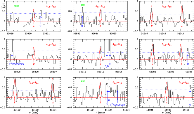
Figure 1: Observed transitions with $K_{a}$ = 0,1 of CH₃CHCO in TMC-1. The abscissa corresponds to the rest frequency of the lines. Frequencies and intensities for the observed lines are given in Table 2. The ordinate is the antenna temperature, corrected for atmospheric and telescope losses, in millikelvin. The quantum numbers of each transition are indicated in the corresponding panel. The red line shows the computed synthetic spectrum for this species for T_rot=9 K and a column density of 1.5$\times$10¹¹ cm^-2. Blanked channels correspond to negative features produced in the folding of the frequency-switching data. Green labels indicate the transitions for which only one of the frequency-switching data points has been used (FS10 and FS8 correspond to a throw of 10 and 8 MHz, respectively). The dotted line in each panel indicates the 3$\sigma$ value.

1 Introduction

The QUIJOTE line survey (Cernicharo et al. 2021a) toward TMC-1 performed in recent years with the Yebes 40m radio telescope has allowed us to detect more than 40 new molecules in space. This underlines the importance of this source for a deep understanding of the different chemical processes in cold dense cores.

Among the latest discoveries, there are several cycles such as cyclopentadiene, indene, ortho-benzyne, or fulvenallene (Cernicharo et al. 2021a, b; Cernicharo et al. 2022). Cyano and ethynyl derivatives of cyclopentadiene (McCarthy et al. 2021; Lee et al. 2021; Cernicharo et al. 2021c) and cyano derivatives of benzene, naphthalene, and indene (McGuire et al. 2018, 2021; Sita et al. 2022) have also been detected. We have also detected propargyl (Agúndez et al. 2021a), one of the most abundant radicals found. Furthermore, long carbon chains such as vinyl acetylene (Cernicharo et al. 2021d), allenyl acetylene (Cernicharo et al. 2021e), butadiynylallene (Fuentetaja et al. 2022a), and ethynylbutatrienylidene (Fuentetaja et al. 2022b) have also been discovered toward TMC-1. Many of these species were not expected because they did not show a high abundance in chemical models. This highlights the importance of further study of the dark cloud TMC-1 in order to understand the chemical processes at work in this kind of environment.

Oxygen-bearing complex organic molecules (COMs) are also an important molecular family present in diverse interstellar environments. The star-forming regions, such as Sgr B2 and Orion KL, are the sources with the highest abundance of COMs. On the contrary, dark clouds like TMC-1 are characterized by carbon-rich chemistry, resulting in long carbon chains with low oxygen content. Agúndez et al. (2021b) reported the detection of O-bearing species, such as CH₂CHCHO, CH₂CHOH, HCOOCH₃, and CH₃OCH₃ in TMC-1. Long carbon chain O-bearing molecules with formulae HC_nO and C_nO (e.g. HC₃O, HC₇O, HC₅O, and C₅O) have also been detected (McGuire et al. 2017; Cordiner et al. 2017; Cernicharo et al. 2021f). O-bearing cations, such as HC₃O⁺ and CH₃CO⁺, have also been recently detected in this source (Cernicharo et al. 2020, 2021g).

In the family of C₃H₄O isomers, the most stable is $trans$-propenal ($trans$-CH₂CHCHO), whose detection was reported by Agúndez et al. (2021b). To date, this is the only isomer in this family detected towards TMC-1. Close in energy, with a difference of 2.8 kJ mol^-1 compared to $trans$-propenal, is methyl ketene (CH₃CHCO). Bermúdez et al. (2018) studied this species in different environments and made a theoretical study of the stability of all C₃H₄O isomers using the coupled cluster (CCSD(T)) ab initio method and the aug-cc-pVTZ basis set. The next member in the series is $cis$-propenal. It is also close in energy to CH₃CHCO, with a difference of 5.8 kJ mol^-1, and therefore it is a candidate for future detection in TMC-1. The last isomer we refer to is cyclopropanone ($c$-H₄C₃O). Its energy is considerably higher than that of the previously named molecules, specifically 78.1 kJ mol^-1 with respect to $cis$-propenal (1 kJ mol^-1=120.3 K), but it is a candidate for detection because the similar and smaller species cyclopropenone ($c$-H₂C₃O) has been reported by Loison et al. (2017).

In this letter we report the first clear detection of CH₃CHCO (methyl ketene) in TMC-1 using the line survey QUIJOTE (Cernicharo et al. 2021a) performed with the Yebes 40m telescope. The formation of this species is investigated in detail using state-of-the-art gas-phase chemical models.

2 Observations

The observational data used in this work are part of QUIJOTE, a spectral line survey of TMC-1 in the Q band carried out with the Yebes 40m telescope at the position $\alpha_{J2000}=4^{\rm h}41^{\rm m}41.9^{\rm s}$ and $\delta_{J2000}=+25^{\circ}41^{\prime}27.0^{\prime\prime}$. The receiver was built within the Nanocosmos project and consists of two cold high-electron mobility transistor amplifiers covering the 31.0–50.3 GHz band with horizontal and vertical polarizations. Receiver temperatures achieved in the 2019 and 2020 runs vary from 22 K at 32 GHz to 42 K at 50 GHz. Some power adaptation in the down-conversion chains have reduced the receiver temperatures during 2021 to 16 K at 32 GHz and 30 K at 50 GHz. The backends are $2\times 8\times 2.5$ GHz fast Fourier transform spectrometers with a spectral resolution of 38.15 kHz, providing the whole coverage of the Q band in both polarizations. A more detailed description of the system is given by Tercero et al. (2021).

The QUIJOTE line survey was carried out in several observing runs between December 2019 and May 2022. All observations are performed using frequency-switching observing mode with a frequency throw of 8 and 10 MHz. The total observing time on the source for data taken with frequency throws of 8 MHz and 10 MHz is 293 and 253 hours, respectively. Hence, the total observing time on source by May 2022 is 546 hours. The measured sensitivity varies between 0.12 mK at 32 GHz and 0.25 mK at 49.5 GHz. The sensitivity of QUIJOTE is around 50 times better than that of previous line surveys in the Q band of TMC-1 (Kaifu et al. 2004). For each frequency throw, different local oscillator frequencies were used in order to remove possible side band effects in the down conversion chain. A detailed description of the QUIJOTE line survey is provided in Cernicharo et al. (2021a).

The main beam efficiency varies from 0.6 at 32 GHz to 0.43 at 50 GHz (Tercero et al. 2021). The telescope beam size is 56^′′ and 31^′′ at 31 and 50 GHz, respectively. The intensity scale used in this work, antenna temperature ($T_{A}^{*}$), was calibrated using two absorbers at different temperatures and the atmospheric transmission model (ATM) (Cernicharo 1985; Pardo et al. 2001). The calibration uncertainties adopted were 10 %. All data were analysed using the GILDAS package.

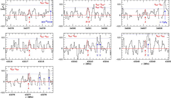
Figure 2: Observed transitions with $K_{a}$ = 2 of CH₃CHCO in TMC-1. The abscissa corresponds to the rest frequency of the lines. Frequencies and intensities for all observed lines are given in Table 2. The ordinate is the antenna temperature, corrected for atmospheric and telescope losses, in milli Kelvin. The quantum numbers of each transition are indicated in the corresponding panel. The red line shows the computed synthetic spectrum for this species for T_rot=9 K and a column density of 1.5$\times$10¹¹ cm^-2. Blanked channels correspond to negative features produced in the folding of the frequency-switching data. The dotted line in each panel indicates the 3$\sigma$ value.

3 Results

Methyl ketene is a nearly prolate molecule having a planar molecular skeleton ($C_{s}$ frame) with only the two hydrogen atoms of the methyl group out of the plane ($C_{3v}$ top), and thus, due to the internal rotation of the methyl top, it belongs to the $G_{6}$ symmetry group. As was shown in the previous rotational analysis of methyl ketene (Bermúdez et al. 2018), its $\rho$ parameter, which accounts for the coupling of the methyl torsion with the overall rotation of the molecule, is relatively high ($\rho=0.196$). For this reason, it was necessary to employ a Hamiltonian aligned to the $\rho$ vector ($\rho$-axis-method, RAM) that accounts for the coupling of the two movements. This employed method is incorporated in the RAM36 software (Rho-axis method for 3- and 6-fold barriers; Ilyushin et al. 2010). The previous model for CH₃CHCO reported by Bermúdez et al. (2018) was slightly adapted to account for the laboratory observed transitions from Bak et al. (1966) and Bermúdez et al. (2018). The model presented in this work also contains the observed transitions in TMC-1 between 32.0 and 50.4 GHz since no lines at those frequencies were accounted for in the previous model. A comparison of the parameters obtained in the previous model (Bermúdez et al. 2018) with the current parameters is presented in Table 1. The parameters of the model have barely changed, showing that the transitions were perfectly incorporated in the fit. Furthermore, for all the observed lines in TMC-1 with $K_{a}=0$ or $1$, the predictions lie within the experimental error. Some transitions of higher $K_{a}$ show slightly higher uncertainty than expected; however, this can be explained by the difficulties of the model to account for the lower energy transitions, already observed in the previous work. These issues are related to the strong coupling of the internal motion and the overall rotation of the molecule, and hence to the high complexity of the model. The dipole moments used in this work, $\mu_{a}$ = 1.65 D and $\mu_{b}$ = 0.33 D, were reported by Bermúdez et al. (2018).

The line identification was achieved using the MADEX catalogue (Cernicharo 2012). We detected a total of 11 lines (divided into $A$ and $E$ components, due to an internal rotation of the methyl group) within the Q band, together with eight lines having an intensity lower than 3$\sigma$. The intensities range from 0.26 to 0.9 mK. The quantum numbers involved range from $J$ = 3 to $J$ = 5 and $K_{a}$ $\leq$ 2. The derived line parameters are given in Table 2. To obtain the column density, we used a model line fitting procedure, with the LTE approach for the thin optical lines (see e.g. Cernicharo et al. 2021d). We obtained $N$(CH₃CHCO)=1.5$\times$10¹¹ cm^-2 with a rotational temperature of 9 K. The models predict the line intensities in antenna temperature taking into account the assumed size of the source to correct for beam dilution, and the beam efficiency of the telescope at the different frequencies of the observations. We assume a source of uniform brightness with a diameter of 80^′′ (Fossé et al. 2001). The H₂ column density for TMC-1 is 10²² cm^-2 (Cernicharo & Guélin 1987), so the abundance of CH₃CHCO is 1.5$\times$10^-11. The predicted synthetic lines for these data are shown in Fig. 1 for $K_{a}$ = 0,1 and in Fig. 2 for $K_{a}$ = 2.

There are several molecules related to CH₃CHCO, so it is interesting to compare their abundances. The most obvious is $trans$-propenal, which is its more stable isomer. The abundance ratio CH₂CHCHO/CH₃CHCO is 1.5. This means that the abundance ratio between the two most stable isomers of the C₃H₄O family is similar to that of the two most stable isomers of the C₂H₄O family, in which case C₂H₃OH/CH₃CHO $\sim$1 (Agúndez et al. 2021b). We can also compare CH₃CHCO with ketene, one of the most abundant O-bearing molecules in TMC-1, with an abundance of 1.4x10^-9 relative to H₂, reported by Cernicharo et al. (2020). This gives an abundance ratio of CH₂CO/CH₃CHCO$\sim$93, which means that the methylated form of ketene is about two orders of magnitude less abundant than ketene itself. Finally, we compared the abundance of methyl ketene with acetaldehyde (CH₃CHO), which has an abundance of 3.5x10^-10 reported by Cernicharo et al. (2020). This gives an abundance ratio of CH₃CHO/CH₃CHCO$\sim$23.

Table 1: Ground torsional state molecular parameters of methyl ketene obtained from the fit using the RAM36 program ($A$-reduction, $I^{r}$-representation).

Parameter	Operator	$n_{op}t_{op}r_{op}$	Previous work (MHz)	This work (MHz)
$A_{RAM}$	$J^{2}_{a}$	$2_{0,2}$	$38587.00(11)$	$38586.91(11)$
$B_{RAM}$	$J^{2}_{b}$	$2_{0,2}$	$4773.813(29)$	$4773.833(27)$
$C_{RAM}$	$J^{2}_{c}$	$2_{0,2}$	$4139.199(46)$	$4139.249(39)$
$D_{ab}$	$\{J_{a},J_{b}\}$	$2_{0,2}$	$-3015.26(39)$	$-3015.62(35)$
$\rho$	$p_{\alpha}J_{a}$	$2_{1,1}$	$0.194354(13)$	$0.194364(12)$
$F$	$p^{2}_{\alpha}$	$2_{2,0}$	$6.4215(13)$	$6.419877(84)$
$V_{3}$	$\frac{1}{2}(1-\cos 3\alpha)$	$2_{2,0}$	$429.38(11)$	$429.2326(32)$
$\Delta_{J}$	$-J^{4}$	$4_{0,4}$	$0.46682(81)\leavevmode\nobreak\ 10^{-2}$	$0.46730(77)\leavevmode\nobreak\ 10^{-2}$
$\Delta_{JK}$	$-J^{2}J^{2}_{a}$	$4_{0,4}$	$-0.17168(62)\leavevmode\nobreak\ 10^{0}$	$-0.17161(59)\leavevmode\nobreak\ 10^{0}$
$\Delta_{K}$	$-J^{4}_{a}$	$4_{0,4}$	$0.47291(60)\leavevmode\nobreak\ 10^{1}$	$0.47296(59)\leavevmode\nobreak\ 10^{1}$
$\delta_{J}$	$-2J^{2}(J^{2}_{b}-J^{2}_{c})$	$4_{0,4}$	$0.15904(40)\leavevmode\nobreak\ 10^{-2}$	$0.15927(38)\leavevmode\nobreak\ 10^{-2}$
$\delta_{K}$	$-2\{J^{2}_{a},(J^{2}_{b}-J^{2}_{c})\}$	$4_{0,4}$	$0.2120(19)\leavevmode\nobreak\ 10^{-1}$	$0.2120(19)\leavevmode\nobreak\ 10^{-1}$
$D_{abJ}$	$\{J_{a},J_{b}\}J^{2}$	$4_{0,4}$	$0.3983(19)\leavevmode\nobreak\ 10^{-1}$	$0.3993(18)\leavevmode\nobreak\ 10^{-1}$
$D_{abK}$	$\{J_{a},J_{b}\}J^{2}_{a}$	$4_{0,4}$	$0.5329(38)\leavevmode\nobreak\ 10^{0}$	$0.5320(36)\leavevmode\nobreak\ 10^{0}$
$\rho_{J}$	$p_{\alpha}J_{a}J^{2}$	$4_{1,3}$	$-0.4253(14)\leavevmode\nobreak\ 10^{0}$	$-0.4254(13)\leavevmode\nobreak\ 10^{0}$
$\rho_{K}$	$p_{\alpha}J^{3}_{a}$	$4_{1,3}$	$0.21648(59)\leavevmode\nobreak\ 10^{2}$	$0.21687(53)\leavevmode\nobreak\ 10^{2}$
$F_{J}$	$p^{2}_{\alpha}J^{2}$	$4_{2,2}$	$0.15159(31)\leavevmode\nobreak\ 10^{0}$	$0.15136(26)\leavevmode\nobreak\ 10^{0}$
$F_{K}$	$p^{2}_{\alpha}J^{2}_{a}$	$4_{2,2}$	$-0.4535(31)\leavevmode\nobreak\ 10^{2}$	$-0.4580(14)\leavevmode\nobreak\ 10^{2}$
$F_{ab}$	$\frac{1}{2}\{J_{a},J_{b}\}p^{2}_{\alpha}$	$4_{2,2}$	$0.902(35)\leavevmode\nobreak\ 10^{0}$	$0.898(30)\leavevmode\nobreak\ 10^{0}$
$V_{3J}$	$J^{2}(1-\cos 3\alpha)$	$4_{2,2}$	$-0.13759(47)\leavevmode\nobreak\ 10^{2}$	$-0.13807(40)\leavevmode\nobreak\ 10^{2}$
$V_{3K}$	$J^{2}_{a}(1-\cos 3\alpha)$	$4_{2,2}$	$-0.1229(28)\leavevmode\nobreak\ 10^{3}$	$-0.1246(27)\leavevmode\nobreak\ 10^{3}$
$V_{3ab}$	$\frac{1}{2}(\{J_{a},J_{b}\})(1-\cos 3\alpha)$	$4_{2,2}$	$-0.647(15)\leavevmode\nobreak\ 10^{2}$	$-0.647(14)\leavevmode\nobreak\ 10^{2}$
$V_{3bc}$	$(J^{2}_{b}-J^{2}_{c})(1-\cos 3\alpha)$	$4_{2,2}$	$0.2134(47)\leavevmode\nobreak\ 10^{1}$	$0.2184(39)\leavevmode\nobreak\ 10^{1}$
$D_{3ac}$	$\frac{1}{2}\{J_{a},J_{c}\}\sin 3\alpha$	$4_{2,2}$	$0.4186(50)\leavevmode\nobreak\ 10^{3}$	$0.4193(49)\leavevmode\nobreak\ 10^{3}$
$\rho_{m}$	$p^{3}_{\alpha}J_{a}$	$4_{1,3}$	$0.514(11)\leavevmode\nobreak\ 10^{2}$	$0.5324(15)\leavevmode\nobreak\ 10^{2}$
$F_{m}$	$p^{4}_{\alpha}$	$4_{4,0}$	$-0.443(15)\leavevmode\nobreak\ 10^{2}$	$-0.46728(72)\leavevmode\nobreak\ 10^{2}$
$V_{6}$	$\frac{1}{2}(1-\cos 6\alpha)$	$4_{4,0}$	$-0.3088(44)\leavevmode\nobreak\ 10^{6}$	$-0.30159(12)\leavevmode\nobreak\ 10^{6}$
$\Phi_{J}$	$J^{6}$	$6_{0,6}$	$0.21428(94)\leavevmode\nobreak\ 10^{-7}$	$0.21471(90)\leavevmode\nobreak\ 10^{-7}$
$\Phi_{JKK}$	$J^{2}J^{4}_{a}$	$6_{0,6}$	$-0.7678(62)\leavevmode\nobreak\ 10^{-4}$	$-0.7686(60)\leavevmode\nobreak\ 10^{-4}$
$\Phi_{K}$	$J^{6}_{a}$	$6_{0,6}$	$0.8161(75)\leavevmode\nobreak\ 10^{-3}$	$0.8154(73)\leavevmode\nobreak\ 10^{-3}$
$\phi_{J}$	$2J^{4}(J^{2}_{b}-J^{2}_{c})$	$6_{0,6}$	$0.9235(85)\leavevmode\nobreak\ 10^{-8}$	$0.9245(80)\leavevmode\nobreak\ 10^{-8}$
$\rho_{JK}$	$p_{\alpha}J^{3}_{a}J^{2}$	$6_{1,5}$	$0.5936(53)\leavevmode\nobreak\ 10^{-3}$	$0.5941(51)\leavevmode\nobreak\ 10^{-3}$
$\rho_{KK}$	$p_{\alpha}J^{5}_{a}$	$6_{1,5}$	$-0.6917(54)\leavevmode\nobreak\ 10^{-2}$	$-0.6895(52)\leavevmode\nobreak\ 10^{-2}$
$F_{JK}$	$p^{2}_{\alpha}J^{2}J^{2}_{a}$	$6_{2,4}$	$-0.1522(14)\leavevmode\nobreak\ 10^{-2}$	$-0.1524(13)\leavevmode\nobreak\ 10^{-2}$
$F_{KK}$	$p^{2}_{\alpha}J^{4}_{a}$	$6_{2,4}$	$0.1585(15)\leavevmode\nobreak\ 10^{-1}$	$0.1578(15)\leavevmode\nobreak\ 10^{-1}$
$V_{3JK}$	$J^{2}J^{2}_{a}(1-\cos 3\alpha)$	$6_{2,4}$	$0.1922(51)\leavevmode\nobreak\ 10^{-1}$	$0.1954(46)\leavevmode\nobreak\ 10^{-1}$
$\rho_{mbc}$	$p^{3}_{\alpha}J_{a}(J^{2}_{b}-J^{2}_{c})$	$6_{3,3}$	$0.677(15)\leavevmode\nobreak\ 10^{-3}$	$0.671(14)\leavevmode\nobreak\ 10^{-3}$
$V_{6ab}$	$\{J_{a},J_{b}\}(1-\cos 6\alpha)$	$6_{4,2}$	$0.425(10)\leavevmode\nobreak\ 10^{2}$	$0.4207(97)\leavevmode\nobreak\ 10^{2}$
$\sigma_{\text{rms}/\text{wrms}}$			$4.42\leavevmode\nobreak\ 10^{-2}/0.74\leavevmode\nobreak\ \leavevmode\nobreak\$	$4.18\leavevmode\nobreak\ 10^{-2}/0.73\leavevmode\nobreak\ \leavevmode\nobreak\$
$Jmax/K_{a}max$			$38/18\leavevmode\nobreak\ \leavevmode\nobreak\ \leavevmode\nobreak\ \leavevmode\nobreak\ \leavevmode\nobreak\ \leavevmode\nobreak\ \leavevmode\nobreak\$	$38/18\leavevmode\nobreak\ \leavevmode\nobreak\ \leavevmode\nobreak\ \leavevmode\nobreak\ \leavevmode\nobreak\ \leavevmode\nobreak\ \leavevmode\nobreak\$
$N_{lines}$			$3040\leavevmode\nobreak\ \leavevmode\nobreak\ \leavevmode\nobreak\ \leavevmode\nobreak\ \leavevmode\nobreak\ \leavevmode\nobreak\ \leavevmode\nobreak\ \leavevmode\nobreak\$	$3059\leavevmode\nobreak\ \leavevmode\nobreak\ \leavevmode\nobreak\ \leavevmode\nobreak\ \leavevmode\nobreak\ \leavevmode\nobreak\ \leavevmode\nobreak\ \leavevmode\nobreak\$

4 Chemical model

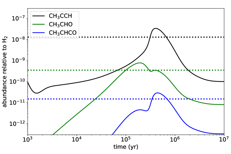
Figure 3: Calculated fractional abundance of CH₃CHCO and its relevant precursors CH₃CCH and CH₃CHO as a function of time. The horizontal dotted line corresponds to the observed abundance in TMC-1.

To investigate the formation of methyl ketene in TMC-1 we carried out gas-phase chemical modelling calculations. The model parameters and chemical network are the same used in Cernicharo et al. (2021g) to model the chemistry of O-bearing molecules following the discovery of HC₃O and C₅O. We added CH₃CHCO as a new species, with a simple chemical scheme of formation and destruction. Although some chemical models (e.g. Garrod et al. 2022) indicate that grain surface processes can help to explain the presence of some complex organic molecules (e.g. methyl formate and dimethyl ether; Agúndez et al. 2021b) in cold sources such as TMC-1, here we aim to evaluate whether purely gas phase processes can account for the formation of CH₃CHCO in TMC-1.

Methyl ketene is not included in the UMIST (McElroy et al. 2013) or KIDA (Wakelam et al. 2015) databases, although some information is available in the NIST Chemical Kinetics database. There are several plausible reactions of formation. The reaction between OH and CH₃CCH is a potential source of methyl ketene because it is relatively rapid at low temperatures, with a measured rate coefficient of 5.08 $\times$ 10^-12 cm³ s^-1 at 69 K (Taylor et al. 2008). However, no information is available on the product distribution, and thus here we assume that CH₃CHCO and H are the main products. The reaction between OH and the non-polar isomer allene (CH₂CCH₂) has also been found to be rapid at low temperatures, although the main products seem to be H₂CCO and CH₃ (Daranlot et al. 2012), and we thus do not include it as a source of methyl ketene. Another reaction that can provide an efficient formation route to methyl ketene is CH + CH₃CHO. This reaction was studied by Goulay et al. (2012), who found that CH₃CHCO is formed with a branching ratio of 0.39. However, the rate coefficient has not been measured, although Wang et al. (2017) studied the reaction theoretically and found that the formation of CH₃CHCO is barrierless. We thus adopted a rate coefficient of 2.41 $\times$ 10^-10 cm³ s^-1, as measured for CH and H₂CO (Hancock & Heal 1992), and the branching ratio measured by Goulay et al. (2012).

There are other reactions that could potentially form CH₃CHCO, although they are unlikely to be efficient in TMC-1. For example, the reaction between HCO and C₂H₄ has a barrier (Lesclaux et al. 1986; Xie et al. 2005a), and the same happens for the reaction between C₂H₃ and H₂CO (Xie et al. 2005b). The reaction between CH₃ and H₂CCO could provide a simple pathway to CH₃CHCO by simply substituting one H atom of ketene by a methyl group, although ketene does not show a high reactivity with radicals. Semenikhin et al. (2018) studied theoretically the reaction between CH₃ and H₂CCO; although they did not consider the formation of CH₃CHCO and H, they found that all the explored channels have barriers. Therefore, we did not include this reaction. Finally, we considered that in TMC-1 methyl ketene is mostly destroyed through reactions with the most abundant cations, such as C⁺, HCO⁺, and H₃O⁺.

The fractional abundance calculated for CH₃CHCO is shown in Fig. 3 as a function of time. It is seen that the peak abundance, reached at a time of some 10⁵ yr, agrees very well with the abundance derived from the observations. The two formation reactions considered here (i.e. OH + CH₃CCH and CH + CH₃CHO) contribute to the formation of methyl ketene. The abundances calculated for CH₃CCH and CH₃CHO are in good agreement with those obtained in Cabezas et al. (2021) and Cernicharo et al. (2020). Further research on the low temperature kinetics and the product distribution of these two reactions will be of great interest to shed light on the origin of methyl ketene in TMC-1.

5 Conclusions

We have presented the first detection of CH₃CHCO towards TMC-1. We used the QUIJOTE line survey taken with the Yebes 40m radiotelescope, with which we observed a total of 11 lines with an intensity higher than 3$\sigma$ and another 8 lines with an intensity lower than 3$\sigma$, involving $J$ = 3 to $J$ = 5 and $K_{a}$ $\leq$ 2. The rotational temperature is 9 K and the derived column density $N$(CH₃CHCO)=1.5$\times$10¹¹ cm^-2. These results imply that methyl ketene is 1.46 less abundant than its most stable isomer (trans-CH₂CHCHO), a value quite similar to the abundance ratio of the isomers vinyl alcohol to acetaldehyde of 1. The observed abundance of methyl ketene is well explained using our gas phase chemical model, considering the formation reactions from propyne and acetaldehyde, and the destruction reactions with the most abundant cations of TMC-1.

Appendix A Observed line parameters

The line parameters derived for this work were obtained by fitting a Gaussian line profile to the observed data, using the software Class (GILDAS package). We use a window of $\pm$ 15 km s^-1 around the V_LSR (5.83km s^-1) of the source for each transition. The results are given in Table 2. The observed lines of methyl ketene are shown in Fig. 1 for $K_{a}$ = 0,1 and in Fig. 2 for $K_{a}$ = 2.

Table 2: Observed line parameters for CH₃CHCO

Transition1	$\nu_{obs}$ a	$\nu_{obs}$-$\nu_{cal}$	$\int T_{A}^{*}dv$ b	$\Delta$vc	$T_{A}^{*}$ d	Notes
	(MHz)	(MHz)	(mK km s-1)	(km s-1)	(mK)
41,4-31,3 $A$	33830.302$\pm$0.010	-0.013	0.51$\pm$0.13	0.98$\pm$ 0.31	0.49$\pm$0.13	A
41,4-31,3 $E$	33834.322$\pm$0.010	0.027	0.49$\pm$0.12	0.66$\pm$ 0.18	0.69$\pm$0.14	B
40,4-30,3 $E$	34545.403$\pm$0.010	0.004	0.58$\pm$0.10	0.75$\pm$ 0.14	0.72$\pm$0.12
40,4-30,3 $A$	34547.083$\pm$0.010	0.007	0.69$\pm$0.11	0.82$\pm$ 0.17	0.78$\pm$0.12
41,3-31,2 $E$	35305.954$\pm$0.022	0.029	0.38$\pm$0.15	0.76$\pm$ 0.35	0.46$\pm$0.14
41,3-31,2 $A$	35313.007$\pm$0.010	0.026	0.51$\pm$0.10	0.69$\pm$ 0.15	0.70$\pm$0.11
51,5-41,4 $A$	42282.025$\pm$0.011	0.007	0.46$\pm$0.16	0.50$\pm$ 0.18	0.86$\pm$0.11
51,5-41,4 $E$	42283.591$\pm$0.013	0.032	0.40$\pm$0.11	0.64$\pm$ 0.19	0.59$\pm$0.11
50,5-40,4 $E$	43158.875$\pm$0.011	-0.020	0.88$\pm$0.14	0.93$\pm$ 0.16	0.89$\pm$0.13
50,5-40,4 $A$	43160.982$\pm$0.010	0.011	0.51$\pm$0.11	0.60$\pm$ 0.13	0.79$\pm$0.13
51,4-41,3 $E$	44129.579$\pm$0.012	0.07	0.33$\pm$0.12	0.48$\pm$ 0.19	0.65$\pm$0.21	A
51,4-41,3 $A$	44134.955$\pm$0.014	0.07	0.53$\pm$0.14	0.63$\pm$ 0.18	0.78$\pm$0.13
42,3-32,2 $A$	34577.168$\pm$0.011	-0.012	0.10$\pm$0.08	0.33$\pm$ 3.42	0.28$\pm$0.16
42,3-32,2 $E$ + 42,2-32,1 $E$	34590.976$\pm$0.015	0.043 & -0.021	0.42$\pm$0.13	0.91$\pm$ 0.26	0.43$\pm$0.12	C
42,2-32,1 $A$	34607.086$\pm$0.010	-0.035	0.11$\pm$0.07	0.35$\pm$ 1.80	0.28$\pm$0.10
52,4-42,3 $A$	43217.244$\pm$0.028	-0.026	0.13$\pm$0.10	0.44$\pm$ 0.34	0.26$\pm$0.15
52,4-42,3 $E$	43242.864$\pm$0.019	0.026	0.19$\pm$0.09	0.58$\pm$ 0.29	0.31$\pm$0.16
52,3-42,2 $E$	43248.485$\pm$0.033	-0.074	0.21$\pm$0.13	0.65$\pm$ 0.35	0.31$\pm$0.22
52,3-42,2 $A$	43277.034$\pm$0.025	-0.071	0.12$\pm$0.09	0.32$\pm$ 0.39	0.36$\pm$0.12