Measuring mass transfer of AM CVn binaries with a space-based gravitational wave detector

Abstract

The formation mechanism of AM CVn binary has not been well understood yet. Accurate measurements of the mass transfer rate can help to determine the formation mechanism. But unfortunately such observation by electromagnetic means is quite challenging. One possible formation channel of AM CVn binary is a semi-detached white dwarf binary. Such system emits strong gravitational wave radiation which could be measured by the future space-based detectors. We can simultaneously extract the mass transfer rate and the orbital period from the gravitational wave signal. We employ a post-Keplerian waveform model of gravitational wave and carry out a Fisher analysis to estimate the measurement accuracy of mass transfer rate through gravitational wave detection. Special attention is paid to the observed sources in Gaia Data Release 2. We found that we can accurately measure the mass transfer rate for those systems. Comparing to electromagnetic observations, gravitational wave detection improves the accuracy more than two orders of magnitude. Our results imply that the gravitational wave detection will help much in understanding the formation mechanism of AM CVn binaries.

1 Introduction

LIGO-VIRGO-KAGRA Collaboration has successfully conducted observation runs 1-3. About 100 gravitational wave (GW) events have been reported. The observation run 4 will start in May 2023 soon. The GW astronomy develops rapidly (Abbott et al. (2016, 2017, 2019, 2021b, 2021a)). The ground-based detectors aim at frequencies above 10 Hz. The space-based gravitational wave interferometers will expand the GW spectrum to lower frequency band ($10^{-4}\sim 1$ Hz). The undergoing space-based detectors include Laser Interferometer Space Antenna (LISA) (Amaro-Seoane et al. (2017)), TianQin (Luo et al. (2016)) and Taiji (Luo et al. (2020); Wang et al. (2020)).

The ultracompact binaries (UCBs) with orbital periods ranging from several minutes to hours are important sources for space-based detectors. Such UCBs include white dwarf binaries (Brown et al. (2020); Burdge et al. (2020)), ultracompact X-Ray binaries (UCXBs) (Chen et al. (2020)) and so forth. Some UCB systems could be observed by both the electromagnetic (EM) means and the GW means. The LISA verification binaries (Kupfer et al. (2018)) belongs to this type including detached white dwarfs, hot subdwarf binaries and AM Canum Venaticorum (AM CVn) systems.

AM CVns are semidetached binaries undergoing helium mass transfer. Their orbital periods range from 5 to 65 minutes (Nelemans (2005)). These systems are ideal laboratories to test tidal interaction models, detonation mechanism, accretion theories (Piro (2019); Ashok & Banerjee (2003); Bildsten et al. (2007); Kotko et al. (2012)), etc. So far, the formation mechanism of AM CVn has remained undetermined. There are three possible channels corresponding donor evolution of He-core white dwarfs (Paczyński (1967); Deloye et al. (2007)), nondegenerate He stars Savonije et al. (1986); Iben & Tutukov (1987); Yungelson (2008) and evolved hydrogen-rich CVs (Tutukov et al. (1985, 1987); Podsiadlowski et al. (2003); Goliasch & Nelson (2015)), respectively. In each channel, the orbit evolution is initially dominated by gravitational wave radiation (GWR). GWR shrink the orbit rapidly until the Roche lobe overflow (RLOF) begins. Subsequently the mass transfer rate (MTR) rises to the peak and tends to dominate the evolution which turns down the orbital frequency increment and eventually makes it decrease. Precise measurement of the donor’s mass transfer rate at a certain orbital period would help us to understand the AM CVn formation mechanism because different channels follow different tracks in $P_{\mathrm{orb}}-\dot{M}_{\mathrm{donor}}$ plane. Nowadays, MTR could be measured through observing bright spots in AM CVn systems. For example, Ramsay et al. (2018) has determined the mass transfer rate for 15 AM CVn stars using Gaia Data Release 2 (Gaia DR2). Furthermore, a large amount of investigations on the Helium transfer have been carried out for double He WD channel (Zhang et al. (2018)), CO+He WD channel (Wong & Bildsten (2021); Chen et al. (2022)) and hot subdwarf B+WD scenario (Bauer & Kupfer (2021)).

LISA verification binaries could be detected with SNR$>$10 based on four year GW observation (Kupfer et al. (2018)). Galactic binary WDs have high SNR and are usually regarded as continuous GW sources. Four year data and appropriate waveform models could make accurate parameter estimations of these sources. For example, LISA could measure the frequency $f$ and its time derivative $\dot{f}$ (Shah et al. (2012)). In semi-detached binaries, $\dot{f}$ is affected by GWR, tidal forces and mass transfer (Kremer et al. (2015)). Therefore, we could extract these parameters including mass transfer rate through matched filtering of GW waveform.

In this paper, we focus on measuring mass transfer in AM CVn systems especially in the white dwarf channel. In next section we express the chirp $\dot{f}$ in terms of frequency $f$ and mass transfer rate $\dot{M}_{\mathrm{donor}}$. Subsequently we carry out a Fisher information analysis for parameter estimation and present the measurability of mass transfer rate in different conditions in Sec. 3. In Sec. 4 we forecast the GW measurement performance in $P_{\mathrm{orb}}-\dot{M}_{\mathrm{donor}}$ plane for several binaries in Gaia DR2 data. At last we conclude our paper in Sec. 5.

2 Waveform model for mass transfer measurement

We adopt the parameterized post-Keplerian gravitational waveform model for the white dwarfs in AM CVn binaries. Within the post-Keplerian waveform model, the orbital elements and their adiabatic variations involve the gravity theories and detailed stellar dynamics (Damour & Taylor (1992)). This approximation is valid especially when the binary seperation is large and consequently the gravitational interaction is weak. Therefore, we could always describe the motion of the binary as a post-Keplerian expansion. The related general gravitational waveform can be expressed as (Willems et al. (2008); Barack & Cutler (2004); Li & Cao (2023)):

$$h^{+}(t) = \sum_{n=1}^{\infty}A\{(1+\cos^{2}\iota)a_{n}(e)\cos[n\phi(t)]\cos(2\gamma)$$ (1)

$$- (1+\cos^{2}\iota)b_{n}(e)\sin[n\phi(t)]\sin(2\gamma)$$

$$+ (\sin^{2}\iota)c_{n}(e)\cos[n\phi(t)]\},$$

$$h^{\times}(t) = -\sum_{n=1}^{\infty}2A\cos\iota\{b_{n}(e)\sin[n\phi(t)]cos(2\gamma)$$ (2)

$$+ a_{n}(e)\cos[n\phi(t)]\sin(2\gamma)\}$$

with

$$a_{n}(e) = n[J_{n-2}(ne)-2eJ_{n-1}(ne)+\dfrac{2}{n}J_{n}(ne)$$ (3)

$$+ 2eJ_{n+1}(ne)-J_{n+2}(ne)],$$

$$b_{n}(e) = n\sqrt{1-e^{2}}[J_{n-2}(ne)-2J_{n}(ne)$$ (4)

$$+ J_{n+2}(ne)],$$

$$c_{n}(e) = J_{n}(ne),$$ (5)

where $J_{n}(z)$ is the $n$th order Bessel function of the first kind and $\iota,~{}e,~{}\gamma$ are inclination angle, orbit eccentricity and periastron direction, respectively. $\phi(t)$ is the Doppler shifted orbital phase

$$\phi(t)=\phi_{0}+\pi ft,$$ (6)

where $f$ is the frequency of the gravitational waves. In order to impose constraints on the number of parameters, we expand GW frequency to the third order of time derivative:

$$f=f_{0}+\dot{f}_{0}t+\dfrac{1}{2}\ddot{f}_{0}t^{2}+\dfrac{1}{6}\dddot{f}_{0}t^{3}.$$ (7)

In the post-Keplerian waveform model, time dependent variables change slowly over time. One could expand these variables adiabatically. The three orbital elements can be written as

$$\iota = \iota_{0}+\dot{\iota}_{0}t,$$ (8)

$$e = e_{0}+\dot{e}_{0}t,$$ (9)

$$\gamma = \gamma_{0}+\dot{\gamma}_{0}t.$$ (10)

For WD binaries which may be affected by the mass transfer, we select circular orbit with $e_{0}=\dot{e}_{0}=0$ and thus $\gamma_{0}=\dot{\gamma}_{0}=0$. These assumptions are reasonable because the progenitors of double white dwarfs may experience several mass transfer phases and tidal forces would circularize the orbit (Willems et al. (2007)). Once the mass transfer starts, tidal forces and gravitational radiation will keep the orbit circular (Kremer et al. (2015)). Therefore, Eqn. (1) and Eqn. (2) can be simplified as

$$h_{+}(t) = 2A_{0}(1+\cos^{2}\iota)\cos[2\phi(t)],$$ (11)

$$h_{\times}(t) = -4A_{0}\cos\iota\sin[2\phi(t)],$$ (12)

with the amplitude

$$A_{0}=\dfrac{(GM_{c})^{5/3}}{c^{4}D_{L}}(\pi f)^{2/3},$$ (13)

where $M_{c}$ is chirp mass and $D_{L}$ is luminosity distance.

Now we take orbital evolution into consideration and assume the loss of angular momentum is only due to the gravitational radiation. We force both stars to remain non-rotating and thus there is no L-S coupling (also called spin-orbit coupling or Russell-Saunders coupling) throughout. The reason why this assumption is selected is that tides could significantly synchronize the two components and transfer the accreted spin angular momentum back to the orbit. Shorter synchronization timescales would help double white dwarfs (DWD) survive mass transfer and would be a better approximation for systems with short orbital periods. (Marsh et al. (2004); Fuller & Lai (2012, 2014)). Observations of GP Com and V396 Hya also exclude the fast-rotating accretor models (Kupfer et al. (2016)). Ignoring L-S coupling means that the direction of the orbital momentum is constant and thus the inclination is invariant over time. Therefore, $\dot{\iota}_{0}$ vanishes.

When one star of the binary expands beyond its Roche lobe, the mass transfer starts and the system becomes semidetached. The star with its Roche lobe filled is called the secondary star. It is also called the donor star. Its mass is traditionally denoted as $M_{2}$. The donor’s companion is called the primary star or accretor whose mass is denoted as $M_{1}$ (Carroll & Ostlie (2017)). On the onset of mass transfer, the donor’s atmospheric gases escape through the inner Lagrangian point $L_{1}$ to the accretor. We assume the mass transfer is conservative which means $\dot{M}=0$ with $M\equiv M_{1}+M_{2}$ and otherwise more parameters would be introduced, such as mass transfer rate induced by stellar winds and efficiency of accretion (Soberman et al. (1997)). In this work, we mainly investigate the measurability of mass transfer in DWDs and the interesting analysis related to detailed mechanisms can be done then. Accordingly we have $\dot{J}_{\mathrm{mass~{}loss}}=0$ for the binary system and the orbital angular momentum loss is only due to the emission of gravitational waves. Hence, the total change of the orbital angular momentum is given by

$$\dot{J}_{\rm orb}=\dot{J}_{\rm GR}.$$ (14)

The orbital angular momentum is written as

$$J_{\rm orb}=\sqrt{\dfrac{Ga}{M}}M_{1}M_{2}$$ (15)

and the change of the orbital angular momentum induced by GWR is given by Landau et al. (2000)

$$\dot{J}_{\rm GR}=-\dfrac{32G^{3}}{5c^{5}}\dfrac{M_{1}M_{2}M}{a^{4}}J_{\rm orb}.$$ (16)

From Eqn. (15), the change of the orbital angular momentum follows

$$\dfrac{\dot{J}_{\rm orb}}{J_{\rm orb}}=(1-q)\dfrac{\dot{M}_{2}}{M_{2}}+\dfrac{\dot{a}}{2a},$$ (17)

where $q\equiv\dfrac{M_{2}}{M_{1}}$. The Eqn. (16) and Eqn. (17) could be combined to obtain the change of semi-major axis of the binary

$$\dfrac{\dot{a}}{2a}=\dfrac{\dot{J}_{\rm GR}}{J_{\rm orb}}-(1-q)\dfrac{\dot{M}_{2}}{M_{2}}.$$ (18)

According to the Kepler’s third law, the frequency of the orbit is

$$f_{\rm orb}=\left(\dfrac{GM}{4\pi^{2}a^{3}}\right)^{1/2}$$ (19)

and the GW frequency is

$$f=2f_{\rm orb}.$$ (20)

The time derivative of $f$ which is called the chirp is given by

$$\dot{f}=-3\dfrac{\dot{a}}{2a}f.$$ (21)

Combining Eqn. (21) with Eqn. (18) and replacing $M_{1},~{}M_{2}$ with $\eta,~{}M_{c}$, the change of the frequency could be written as

$$\dot{f}=\dot{f}_{\rm 0PN}(1+\Delta_{\rm 1PN}f^{2/3})+\Delta_{\rm MT}f.$$ (22)

with

$$\dot{f}_{\rm 0PN} = \dfrac{96}{5}\dfrac{(GM_{c})^{5/3}\pi^{8/3}}{c^{5}}f^{11/3},$$ (23)

$$\Delta_{\rm 1PN} = -\left(\dfrac{743}{336}+\dfrac{11}{4}\eta\right)\left(\dfrac{\pi M_{c}G}{\eta^{3/5}c^{3}}\right)^{2/3},$$ (24)

$$\Delta_{\rm MT} = \dfrac{6\sqrt{1-\eta}}{M_{c}\eta^{2/5}}\dot{M}_{2},$$ (25)

where $\eta=\dfrac{M_{1}M_{2}}{M^{2}}$ is the symmetric mass ratio and $M_{c}$ is the so-called chirp mass $M_{c}\equiv(M_{1}M_{2})^{3/5}M^{-1/5}$. The first term of Eqn. (22) is the leading order in the post Newtonian expansion and the second term is the next-to-leading order which depends on mass ratio as well (Arun et al. (2005)). The third term is due to mass transfer and mass transfer rate is set to be negative, $\dot{M}_{2}<0$. Similarly, the second and the third time derivatives of GW frequency $f$ are given by

$$\ddot{f} = \dfrac{11}{3}\dfrac{\dot{f}_{\rm 0PN}^{2}}{f}\left(1+\dfrac{24}{11}\Delta_{\rm 1PN}f^{2/3}\right)+\left.\dfrac{14}{3}\Delta_{\rm MT}\dot{f}_{\rm 0PN}\right(1$$ (26)

$$+ \left.\dfrac{8}{7}\Delta_{\rm 1PN}f^{2/3}\right)+\Delta_{\rm MT}^{2}f,$$

$$\dddot{f} = \dfrac{209}{9}\dfrac{\dot{f}_{\rm 0PN}^{3}}{f^{2}}\left(1+\dfrac{713}{209}\Delta_{\rm 1PN}f^{2/3}\right)+\dfrac{121}{3}\dfrac{\Delta_{\rm MT}\dot{f}_{\rm 0PN}^{2}}{f}$$ (27)

$$\cdot \left(1+\dfrac{366}{363}\Delta_{\rm 1PN}f^{2/3}\right)+\left.\dfrac{163}{9}\Delta_{\rm MT}^{2}\dot{f}_{\rm 0PN}\right(1$$

$$+ \left.\dfrac{217}{164}\Delta_{\rm 1PN}f^{2/3}\right)+\Delta_{\rm MT}^{3}f.$$

In the detector frame the waveform can be expressed as (Willems et al. (2008))

$$h=\dfrac{\sqrt{3}}{2}[F_{+}h^{+}+F_{\times}h^{\times}]$$ (28)

where $F_{+},~{}F_{\times}$ are pattern functions of the detector

$$F_{+} = \dfrac{1}{2}(1+\sin^{2}\theta)\cos 2\phi\cos 2\psi$$ (29)

$$- \sin\theta\sin 2\phi\sin 2\psi,$$

$$F_{\times} = \dfrac{1}{2}(1+\sin^{2}\theta)\cos 2\phi\sin 2\psi$$ (30)

$$+ \sin\theta\sin 2\phi\cos 2\psi.$$

In the current work, we focus on the effects of the mass transfer and thus we can ignore the source localization and the wave polarization. Therefore we fix $\phi=\psi=0$ and $\theta=\pi/2$ and thus the pattern functions are equivalent to sky-averaging pattern functions when source position coincides with the specific direction. We assume that intrinsic parameters are independently of the precise location of the source as well as the orientation of the spacecraft and thereby we average over the pattern functions which could be written as

$$F_{+}=1,~{}~{}F_{\times}=0.$$ (31)

Hence, we only consider 6 intrinsic parameters($A,~{}f_{0},~{}q,~{}M_{c},~{}\dot{M}_{2},\\ ~{}\phi_{0}$). In order to avoid parameter degeneracy, we use $A$ to replace $2A_{0}(1+\cos^{2}\iota)$. In the following we can use matched filtering to estimate the waveform parameter $\dot{M}_{2}$.

3 Parameter Estimation

We use Fisher information analysis to estimate the measurement accuracy of the aforementioned waveform parameters. Fisher information techniques have been used to estimate measurement accuracy in many works (see e.g. Cutler (1998), Shah et al. (2012), Shah & Nelemans (2014) and Wolz et al. (2021)). For large signal to noise ratio $S/N$, the parameter-estimation errors have the Gaussian probability distribution (Cutler (1998)) and then the Fisher information matrix (FIM) could provide the GW parameter measurement errors based on appropriate gravitational wave templates. The measurement uncertainty of the parameters $\lambda^{i}$ at $1\sigma$ confidence is given by the inverse of the FIM $\Gamma_{ij}$

$$\Delta\lambda^{i}=\sqrt{\Gamma^{-1}_{ii}},$$ (32)

where $\Gamma_{ij}$ is defined by

$$\Gamma_{ij}=\left(\left.\dfrac{\partial h}{\partial\lambda^{i}}\right|\dfrac{\partial h}{\partial\lambda^{j}}\right).$$ (33)

The inner product $(~{}|~{})$ is defined as (Finn (1992))

$$(a(t)|b(t))=4\Re\int_{0}^{\infty}\dfrac{\tilde{a}^{*}(f)\tilde{b}(f)}{S_{n}(f)}df,$$ (34)

where the asterisk denotes complex conjugation, the tilde denotes the Fourier transformation and $S_{n}$ is the spectral noise density of the detector. Since within the time of observation the signal of the white dwarf binaries could be treated as monochromatic, we make an approximation of $S_{n}(f)\approx S_{n}(f_{0})$ and Eqn. (34) could be turned into time integral (Wolz et al. (2021))

$$(a|b)=\dfrac{2}{S_{n}(f_{0})}\int_{0}^{T_{\rm obs}}a(t)b(t)dt.$$ (35)

The sensitivity curve of LISA is given by Robson et al. (2019):

$$S_{n}(f) = \dfrac{10}{3L^{2}}\left(P_{\mathrm{OMS}}+2(1+\cos^{2}(f/f_{*}))\dfrac{P_{\mathrm{acc}}}{(2\pi f)^{4}}\right)$$ (36)

$$\times \left(1+\frac{6}{10}\left(\dfrac{f}{f_{*}}\right)^{2}\right),$$

$$f_{*} = c/(2\pi L),$$ (37)

$$P_{\mathrm{OMS}} = (1.5\times 10^{-11}\mathrm{m})^{2}\mathrm{Hz}^{-1},$$ (38)

$$P_{\mathrm{acc}} = \left(3\times 10^{-15}\mathrm{m~{}s^{-2}}\right)^{2}$$ (39)

$$\times \left[1+\left(\dfrac{4\times 10^{-4}\mathrm{Hz}}{f}\right)^{2}\right]\mathrm{Hz}^{-1},$$

$$L = 2.5\times 10^{9}\mathrm{m}.$$ (40)

The observation time is chosen to be maximal running time of the satellites which is $T_{\mathrm{obs}}=10$ years.

4 Mass transfer rate estimation

In the following we firstly investigate the detectability of AM CVn’s mass transfer rate. After that we pay special attention to the semi-detached systems. The known verification binaries of LISA belongs to this type and they may undergo mass transfer phase. Although GW observation data on them have not been obtained so far, mass transfer rates in white dwarfs binary simulations and optical observation results are used for parameter estimation.

4.1 Detectability

The WD scenario of AM CVn consists of a degenerate, low mass He WD with the mass ranging from 0.1 $M_{\odot}$ to 0.2 $M_{\odot}$ and a 0.6-1.0 $M_{\odot}$ carbon-oxygen WD (Wong & Bildsten (2021)). We present the GW measurement results of MTRs in a white dwarf binary with individual masses of $m_{1}=0.75M_{\odot}$, $m_{2}=0.15M_{\odot}$. In addition we set observation frequency $f_{0}=5\times 10^{-3}$ Hz, the orbital inclination $\iota=\dfrac{\pi}{2}$ and the initial phase $\phi_{0}=0$ as fiducial values. We vary the mass transfer rate $\dot{M}_{2}$ and the luminosity distance $D_{L}$ in order to discuss the measurement accuracy of $\dot{M}_{2}$ with LISA.

Neglecting the dynamical evolution of the stellars, the measurement error at 1 $\sigma$ is a function of the MTR of the system and the luminosity distance. As shown in Fig. 1, we vary the MTR from $10^{-14}~{}M_{\odot}/\mathrm{yr}$ to $10^{-6}~{}M_{\odot}/\mathrm{yr}$ and the luminosity distance $D_{L}$ among the range $10^{2}\sim 10^{6}$ pc in the $\dot{M_{2}}-D_{L}$ parameter plane. The detectability could be described by two indicators including the SNR and the measurement errors. For a given detector, the SNR is directly associated with the signal amplitudes which are inversely proportional to the luminosity distance. At luminosity distance $D_{L}=6.68\times 10^{4}$ pc, the SNR is about $10$. When $D_{L}>1.34\times 10^{5}$pc, the SNR would decrease below about 5. We select $10^{5}$ pc as the maximum detectable range. Denoting the measurement error of MTR as $\Delta\dot{M}_{2}$, we regard $\Delta\dot{M}_{2}/\dot{M}_{2}<1$ as measurable. $\Delta\dot{M}_{2}/\dot{M}_{2}=1$ corresponds to the black solid line plotted in Fig. 1. For a WD binary, if time derivative of frequency is negative, or to say, the orbital period is increasing, the system is dominated by astrophysical effects other than the GWR. According to the currently known AM CVn systems ($P_{\rm orb}\sim 5-65$ min) with periods increasing, the source distances are distributed between several hundred and two thousand parsecs and the MTR ranges from $10^{-12}M_{\odot}/\mathrm{yr}$ to $10^{-7}M_{\odot}/\mathrm{yr}$ (see Ramsay et al. (2018) for more information). When the distance is around $10^{3}$ pc, we could measure the MTR accurately if only $\dot{M}_{2}>5\times 10^{-13}M_{\odot}/\mathrm{yr}$. When the He WD donor fills its Roche lobe, the MTR rapidly peaks to $10^{-7}\sim 10^{-8}M_{\odot}/\mathrm{yr}$ within $10^{6}$ yrs and then decreases as $t^{-1.3}$ (Bildsten et al. (2006)). The other two important distances are 8 kpc and 20 kpc which are distances of sources in galactic center and edge of the population estimated by Kremer et al. (2017). At the galactic boundary, the MTR could be measured precisely if $\dot{M}_{2}>6\times 10^{-12}M_{\odot}/\mathrm{yr}$ and at the center, the threshold is $3\times 10^{-12}M_{\odot}/\mathrm{yr}$. Therefore, the GW measurement abilities of the MTR in WD channel of AM CVn systems can almost cover the whole stage from the onset of mass transfer to the end of evolution. Additionally, we found that the measurability depends on initial frequency $f_{0}$. For most galactic AM CVn systems with long periods, such as $P_{\rm orb}\sim 65$ min corresponding to $f_{0}\sim 5\times 10^{-4}$ Hz, the mass transfer rate could still be measurable when it’s large enough to exceed $10^{-10}M_{\odot}/\rm yr$. Since the normal mission lifetime is 4 years, here we depicts the measurement threshold to be the fine solid line in Fig. 1. Results show that at the distance of $10^{3}$ pc, we could measure the MTR with high accuracy if $\dot{M}_{2}>4\times 10^{-12}M_{\odot}/\rm yr$ within a 4-year observation. And at the boundary and center of the Milky Way galaxy, the threshold are $8\times 10^{-11}M_{\odot}/\rm yr$ and $3\times 10^{-11}M_{\odot}/\rm yr$, respectively.

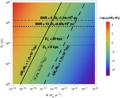
Figure 1: Measurement error of the mass transfer rate $\Delta\dot{M}_{2}$ at fiducial frequency $f_{0}=5\times 10^{-3}$ Hz with a 10-year observation of LISA. The detection threshold is constrained by the black solid line ($\Delta\dot{M}_{2}/\dot{M}_{2}$) and the dot dashed line (SNR). The black solid line represents $\Delta\dot{M}_{2}/\dot{M}_{2}=1$ and the dot dashed line corresponds to the SNR under 5 corresponding to the maximum detectable range $1.34\times 10^{5}$ pc. The black dashed line indicates that the SNR $=10$ at $6.68\times 10^{4}$ pc. Double white dwarfs in the galactic center and the population edge have distances of 8 kpc and 20 kpc which are plotted as dotted lines. For comparison, we present the threshold for WD binaries at observation frequency $f_{0}=5\times 10^{-4}$ Hz which is corresponding to the orbital period, $P_{\rm orb}=65$ min. When the observation time is set to be 4 years, the detection threshold at the frequency $f_{0}=5\times 10^{-3}$ Hz is depicted to be the fine line.

4.2 Applications

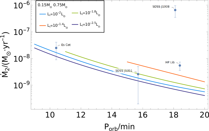
Figure 2: Optical observations of mass transfer rate for AM CVn systems reported by Gaia DR2 among the LISA verification binaries (Ramsay et al. (2018)). These systems are ES Cet, SDSS J1351-0643, SDSS J1908+3940 and HP Lib with respectively periods 10.4, 15.7, 18.1, 18.4 minute and distances 1584, 1317, 1044, 276 pc. The colored lines are the evolution of double white dwarfs of $m_{1}=0.75M_{\odot}$, $m_{2}=0.15M_{\odot}$ with different initial luminosities of the donor. Higher luminosity means less internal material degeneracy and larger radius which induces mass transfer start at longer periods.

Next we will discuss the applications to realistic astrophysical problems. In current optical observations, reliable values of mass transfer rate require a wide-band spectrum. Using Gaia DR2, Ramsay et al. (2018) have determined the mass transfer rate for 15 AM CVn stars. Four of these sources are LISA verification binaries which are expected to emit detectable GW signals (Kupfer et al. (2018)), as shown in Fig. 2. They are ES Cet, SDSS J1351-0643, SDSS J1908+3940 and HP Lib respectively with periods 10.4, 15.7, 18.1, 18.4 minute and distances 1584, 1317, 1044, 276 pc. The mass transfer rate of these AM CVn systems is important to distinguish three possible formation channels. Different channel follows different tracks in the $P_{\mathrm{orb}}-\dot{M}_{\mathrm{donor}}$ plane. This is because the mass transfer rate $\dot{M}_{\mathrm{donor}}$ depends on the donor’s mass-radius relation which is determined by its internal material degeneracy and thermal evolution (Deloye et al. (2007)).

The over-fill of the Roche lobe is defined as (Marsh et al. (2004)):

$$\Delta=R_{\mathrm{donor}}-R_{L},$$ (41)

where $R_{L}$ is the radius of the Roche lobe. Eggleton (1983)’s approximation for the Roche lobe radius gives the expression as

$$R_{L}=a\frac{0.49q^{2/3}}{0.6q^{2/3}+\ln(1+q^{1/3})},$$ (42)

where $a$ is the semi-major axis. When $R_{L}$ is obtained, the binary period could be determined through $\Delta=0$.

After the mass transfer begins, $\dot{M}_{\mathrm{donor}}$ will peak within $10^{6}$ yrs. More degenerate donors have higher peak $\dot{M}$ and lower $\dot{M}$ at a given age due to the smaller radii (Kaplan et al. (2012)). Comparing to a He star, a WD is more degenerate. And thus the two tracks in the $P_{\mathrm{orb}}-\dot{M}_{\mathrm{donor}}$ plane are different. We evolve double white dwarfs with masses $M_{1}=0.75M_{\odot}$, $M_{2}=0.15M_{\odot}$, using binary of Modules for Experiments in Stellar Astrophysics (MESA, v12778; Paxton et al. (2011); Paxton et al. (2013, 2015, 2018, 2019)). To construct a He WD and a C/O WD, we evolve a 1.5$M_{\odot}$ and a 4$M_{\odot}$ zero-age main-sequence star respectively with metallicity of $Z=0.02$ until He cores reach to the required masses, $0.15M_{\odot}$ and $0.75M_{\odot}$ respectively. And then the hydrogen envelope is stripped with high mass loss rate. Eventually, we evolve the bare He core to $\log(L/L_{\odot})=-2$ (Zhang et al. (2018)) alongside the WD cooling track, avoiding helium ignition. In order to investigate stars with different degeneracy, we let the cooling tracks evolve to $\log(L/L_{\odot})=-1.4,~{}-1.8,~{}-2.5$ as initial luminosity. As shown in Eqn. (22), GWR always leads the orbital frequency to increase and the mass transfer term is the opposite. We focus on the stage where the orbital period is increasing, corresponding to the negative time derivative of the frequency, $\dot{f}<0$. In this phase we are sure that the mass transfer effect has been involved in the binary evolution and then could be measured. In the WD cooling track, materials of the He star with higher luminosity are less compact and the radius is larger. Therefore the donor enters mass transfer at earlier stage with a longer period. Then we analyze the GW measurement of these sources. Fig. 3 presents the results of GW measurement errors of the MTR and the period given by FIM based on LISA. Since there have been no GW data yet, we use the photometric results and MESA simulations to set the system parameters and other required orbital parameters are given by Ramsay et al. (2018). In Table 1, we show the GW measurement uncertainties of the four sources’ periods and mass transfer rates. We also show optical measurement errors which are obtained from Gaia DR2 (Ramsay et al. (2018)). Results indicate that GW measurement accuracy could improve more than four orders of magnitude comparing to optical observations for those sources which have relatively large mass transfer rate, such as Es Cet. Even for distant sources with small mass transfer rate, the improvement could also reach more than two orders of magnitude. GW detections could measure both mass transfer rate and frequency of a certain white dwarf binary at a level of high accuracy and especially the errors of period are $O(10^{-7})$ minute. Hence future GW measurements would make a significant contribution to improve resolutions in the $P_{\mathrm{orb}}-\dot{M}_{\mathrm{donor}}$ plane. According to such information we can easily distinguish the formation channel of AM CVns.

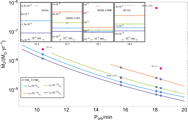
Figure 3: GW measurement errors of the MTR and the period estimated by FIM based on LISA for ES Cet, SDSS J1351-0643, SDSS J1908+3940 and HP Lib. We use orbital period of these sources and the corresponding mass transfer rate got by our MESA simulations to make the parameter estimation. We have also zoomed in the regions of measurement at scales of $O(10^{-6})$ and $O(10^{-7})$ minute to illustrate the GW measurement accuracy.

Table 1: GW measurement uncertainties of orbital periods and mass transfer rates. The values and optical measurement errors of the two parameters are from Gaia DR2 (Ramsay et al. (2018)).

Source	Distance	$P_{\rm orb}$	$\Delta P_{\rm orb,~{}GW}$	$\dot{M}_{2}$	$\Delta\dot{M}_{2,~{}\rm GW}$	$\Delta\dot{M}_{2,~{}\rm Gaia~{}DR2}$
	(pc)	(mins)		$(M_{\odot}\rm yr^{-1})$
Es Cet	1584	10.4	$8.9\times 10^{-8}$	$2.5\times 10^{-8}$	$2.0\times 10^{-12}$	$1.6\times 10^{-8}$
SDSSJ1351	1317	15.7	$6.2\times 10^{-7}$	$2.6\times 10^{-9}$	$4.9\times 10^{-12}$	$2.4\times 10^{-9}$
SDSSJ1908	1044	18.1	$1.1\times 10^{-6}$	$6.6\times 10^{-7}$	$5.9\times 10^{-12}$	$3.1\times 10^{-7}$
HP Lib	276	18.4	$3.0\times 10^{-7}$	$5.5\times 10^{-9}$	$1.7\times 10^{-12}$	$1.9\times 10^{-9}$

5 Conclusions

In this work, we perform a FIM analysis to investigate the measurement of mass transfer rate in WD channel of AM CVn systems using space based GW detectors such as LISA. We assume the loss of orbital angular momentum is only due to the gravitational radiation and introduce mass transfer rate into time derivative of orbital frequency. For a typical AM CVn system with masses of $0.15M_{\odot}-0.75M_{\odot}$ and frequency of $5\times 10^{-3}$ Hz, we found that GW detection of mass transfer rate could extend the distance to $10^{5}$ pc (SNR $>5$). For the known AM CVn systems with distances about kpc, the mass transfer rate could be measured as accurate as $5\times 10^{-13}M_{\odot}$/yr. For Milky Way mass-transfering DWDs with SNR $>10$, based on LISA observation, the mass transfer rate could be measured with accuracy $6\times 10^{-12}M_{\odot}$/yr. The numbers of such LISA resolvable semi-detached binaries estimated by most binary population synthesis are several thousands, even though the numbers vary with different binary evolution models (Nelemans et al. (2001); Kremer et al. (2017); Breivik et al. (2018)). The GW measurement could cover the early mass transfer phases and the stage $\dot{M}_{\mathrm{donor}}$ peaks. Moreover, surveys by GW could be carried out for sources within 100 kpc. And consequent joint observations with electromagnetic band can be done. The survey could also test accretion theories based on the observation of Milky Way known sources. Such observation can also enlarge the mass transfering binary population.

The three possible channels of AM CVn system formation differ largely in donor star’s property especially the donor’s mass-radius relationship. we evolve double white dwarfs of $0.15M_{\odot}-0.75M_{\odot}$ using MESA. Initially we cool a bare He core to $\log(L/L_{\odot})=-2$ as a standard WD following Zhang et al. (2018)’s procedure. We investigated several luminosities in order to investigate different material compactness. Ramsay et al. (2018) have extracted 15 AM CVn stars’ mass transfer rate from Gaia DR2 dataset and found they are greater than $P_{\rm orb}-\dot{M}_{\rm donor}$ tracks of a hot donor star predicted by Bildsten et al. (2006). We analyzed four of them which are within LISA verification binaries. Using these optical observations and evolution tracks as input values for FIM, we found that the GW measurement could reduce the error bars of mass transfer rate by at least one order of magnitude and the error bars of orbital period to $O(10^{-7})$ minute. Improvements of the “resolution” in the $P_{\mathrm{orb}}-\dot{M}_{\mathrm{donor}}$ plane would significantly help recognize the donor’s physical property and exclude evolution models. In current observations, detection for white dwarfs especially for mass transfer rate requires photometric information in a wide range spectrum extending to ultraviolet band (Ramsay et al. (2005, 2006)). However, cool white dwarfs with low luminosity are difficult to be measured. Detection by GW performs as a new means to discover cool donors with low luminosity during mass transfer, independent of photometric information and may thereby overcome the limitation of optical observations in the near future.

The discussions are mainly based on increasing orbital period stage ($\dot{f}<0$) and we have possibility of mistaking mass transfering double white dwarfs for detached systems when $\dot{f}>0$. To some extent, we could recognize mass transfer effects in a maximum run time of ten years. The differences between semi-detached and detached binaries could be described by Eqn. (22) and the second term would be removed in detached systems. Two sets observation of $f$ and $\dot{f}$ are required: the first year observation result (denoted with subscript of “$i$”) and the last year observation result (denoted with subscripts of “$l$”). We could evolve the first term in Eqn. (22) with initial values of $f_{i}$ and $\dot{f}_{i}$ for ten years and obtain evolved final values $f^{\prime}_{l}$. Imposing the observed values to FIM, measurement errors $\Delta f_{i}$ and $\Delta f_{l}$ are obtained. If $\mid f^{\prime}_{l}-f_{l}\mid>\mid\Delta f_{i}+\Delta f_{l}\mid$, we are still sure that the binary is dominated by some astro-effects, such as mass transfer and L-S coupling, since the frequency and its time derivative could be measured accurately by LISA (Shah et al. (2012)). $\dot{f}>0$ represents early mass transfer stage where the mass transfer rate history remains a large amount of uncertainties so far. Extracting mass transfer rate of this phase and reconstructing the evolution tracks are interesting when the GW detection is available.

Data Availability

The data underlying this article will be shared on reasonable request to the corresponding author.

Appendix A Variance-covariance matrix and numerical stability

In this appendix, we discuss the numerical stability of the FIM analysis involved in the main text. We firstly list the full variance-covariance matrix (VCM) in Table. 2 for the measurement of a set of semi-detached white dwarf binary parameters. The system is a typical AM CVn system with their representative parameter values among this population. The first row lists six parameters, with their respective values provided in the second row. The diagonal elements are absolute uncertainties of each parameter and off-diagonal elements are normalized correlations. As shown in Table. 2, strong correlations are marked in bold.

The results of VCM reveals that the set of parameters ($\dot{M}_{2},~{}M_{c},~{}q$) which define the frequency derivative are highly correlated or anti-correlated. The reason for this is that the frequency changes are limited within a runtime of observation and the signals appear to be similar alongside the gradients of these three parameters. In order to demonstrate reliablility of measurements, two-dimensional $1~{}\sigma$ error ellipses are shown in Fig.4. The elongated error ellipses indicate a relatively high degree of parameter degeneracy. However, it is worth noting that the ellipses imply that there are still discernible variations and constraints that can be used to make measurements of the parameters.

Stabilization of the variance covariance matrix could usually be checked by whether the results are consistent when using different levels of accuracy in numerical derivatives (Shah et al. (2012)). In this work, we carried out the analytical expression of derivatives and thereby avoid numerical uncertainties in derivatives. Typically, an unstable FIM implies that small changes in the values of parameters can result in large changes in the estimated parameters and leads to large uncertainties in one or more parameters. Here, numerical uncertainties could only come from numerical integrations. Since the selected integration method is ‘GlobalAdaptive’ in MATHEMATICA, numerical errors of integrations are influenced by working precisions. Therefore, working precisions are varied by 7 levels corresponding to the different numerical errors for integrations in FIM, where the average relative errors $\delta_{i=1,\dots 7}=(2.78\times 10^{-6},~{}1.62\times 10^{-7},~{}1.36\times 10^{-7},~{}9.93\times 10^{-8},~{}3.79\times 10^{-8},~{}3.66\times 10^{-8},~{}5.80\times 10^{-9})$. Here we use Maselli et al. (2022)’s method to check numerical stabilization. Figure 5 (a) shows the maximum relative error, $|\Gamma_{kl}(\delta_{i})/\Gamma_{kl}(\delta_{j})-1|\times 100$, computed by using different working precisions of integrations. Results indicate that the Fisher matrices computed by different working precisions differ less than $10^{-5}$. Since it’s well known that if the parameters are highly correlated, the adding parameters would dilute the available information and computing the inverse of the Fisher matrix could be numerically difficult. Therefore we apply a truncated singular value decomposition (SVD) approach on $\Gamma$ (Berti et al. (2005); Pai & Arun (2013)) and we decompose the Fisher matrix $\Gamma$ as

$$\Gamma=USV^{T},$$ (43)

where $U,~{}V$ are orthogonal and $S$ is diagonal, $S={\rm diag}(s_{1},~{}s_{2},\dots s_{n})$, with sigular values $s_{i}\geq 0$. And then the inverse of $\Gamma$ is given by

$$\Gamma^{-1}=VS^{-1}U^{T}.$$ (44)

In this way, we replace the $1/s_{i}$ by zero when $s_{i}$ approximates to zero in Eq. (43) and eventually obtain a “pseudoinverse” of the Fisher matrix which is close to the “real” inverse. Figure 5 (b) shows the maximum relative error between the square root of the diagnoal components of the covariance matrices. Results imply SVD approach helps stabilize the correlation coefficients with differences smaller than $10^{-9}$.

Table 2: A typical AM CVn systems with SNR$\sim$321.41.

	$A$	$f$	$\dot{M}_{2}$	$M_{c}$	$\eta$	$\phi_{0}$
	$5.746\times 10^{-23}$	$2\times 10^{-3}$Hz	$10^{-8}M_{\odot}/\mathrm{yr}$	$0.2753M_{\odot}$	0.1449	0
$A$	$3.209\times 10^{-25}$	-0.1075	-0.1202	$9.243\times 10^{-2}$	0.1202	$8.272\times 10^{-2}$
$f$		$3.889\times 10^{-11}$	0.9682	-0.9681	-0.9682	-0.8660
$\dot{M}_{2}$			$4.319\times 10^{-12}$	-0.9996	-0.9999	-0.7453
$M_{c}$				$1.024\times 10^{-4}$	0.9996	0.7452
$\eta$					$5.551\times 10^{-5}$	0.7453
$\phi_{0}$						$8.341\times 10^{-3}$

Figure 4: Two-dimensional error ellipses of $\ln\dot{M}_{2},~{}\ln M_{c},~{}q$, for a typical AM CVn system. The black solid lines represent $1-\sigma$ ellipses.

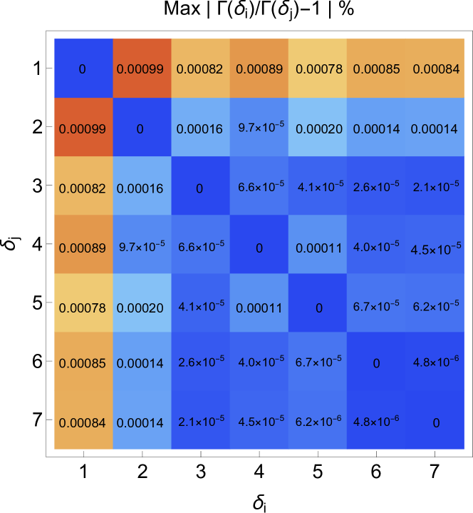
(a)

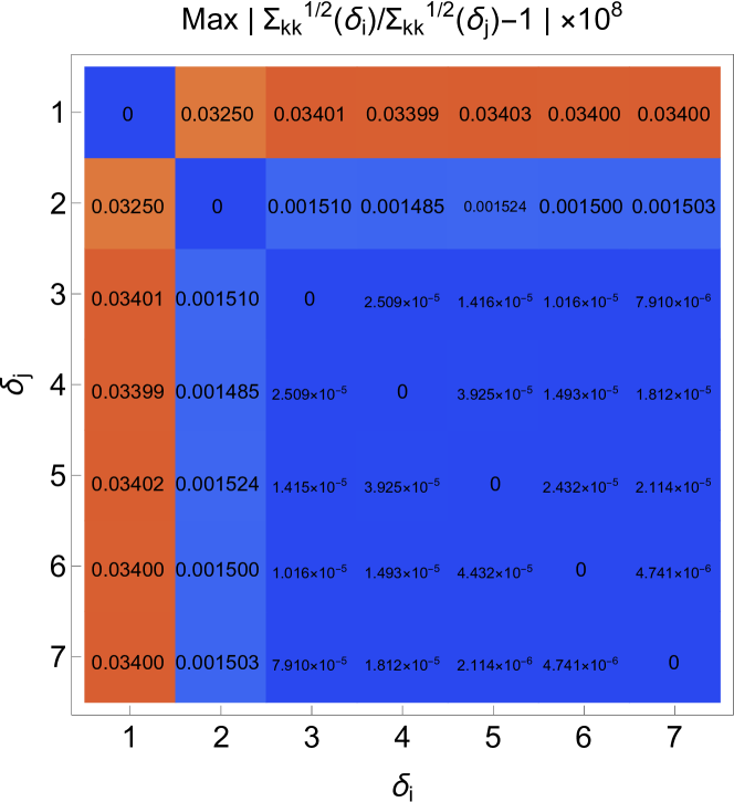
(b)

Figure 5: Maximum relative errors between Fisher matrices computed by different working precisions of integration (left) and maximum relative errors between square root of the diagonal components of the covariance matrices (right).

References

- Abbott et al. (2016) Abbott B. P., et al., 2016, Phys. Rev. Lett., 116, 061102
- Abbott et al. (2017) Abbott B. P., et al., 2017, Phys. Rev. Lett., 119, 161101
- Abbott et al. (2019) Abbott B. P., et al., 2019, Phys. Rev. X, 9, 031040
- Abbott et al. (2021a) Abbott R., et al., 2021a, arXiv e-prints, p. arXiv:2111.03606
- Abbott et al. (2021b) Abbott R., et al., 2021b, Phys. Rev. X, 11, 021053
- Amaro-Seoane et al. (2017) Amaro-Seoane P., et al., 2017, arXiv e-prints, p. arXiv:1702.00786
- Arun et al. (2005) Arun K. G., Iyer B. R., Sathyaprakash B. S., Sundararajan P. A., 2005, Physical Review D, 71, 084008
- Ashok & Banerjee (2003) Ashok N. M., Banerjee D. P. K., 2003, Astronomy & Astrophysics, 409, 1007
- Barack & Cutler (2004) Barack L., Cutler C., 2004, Physical Review D, 69, 082005
- Bauer & Kupfer (2021) Bauer E. B., Kupfer T., 2021, The Astrophysical Journal, 922, 245
- Berti et al. (2005) Berti E., Buonanno A., Will C. M., 2005, Physical Review D, 71, 084025
- Bildsten et al. (2006) Bildsten L., Townsley D. M., Deloye C. J., Nelemans G., 2006, The Astrophysical Journal, 640, 466
- Bildsten et al. (2007) Bildsten L., Shen K. J., Weinberg N. N., Nelemans G., 2007, The Astrophysical Journal, 662, L95
- Breivik et al. (2018) Breivik K., Kremer K., Bueno M., Larson S. L., Coughlin S., Kalogera V., 2018, The Astrophysical Journal Letters, 854, L1
- Brown et al. (2020) Brown W. R., et al., 2020, The Astrophysical Journal, 889, 49
- Burdge et al. (2020) Burdge K. B., et al., 2020, The Astrophysical Journal, 905, 32
- Carroll & Ostlie (2017) Carroll B. W., Ostlie D. A., 2017, An Introduction to Modern Astrophysics, 2 edn. Cambridge University Press, doi:10.1017/9781108380980
- Chen et al. (2020) Chen W.-C., Liu D.-D., Wang B., 2020, The Astrophysical Journal Letters, 900, L8
- Chen et al. (2022) Chen H.-L., Chen X., Han Z., 2022, The Astrophysical Journal, 935, 9
- Cutler (1998) Cutler C., 1998, Phys. Rev. D, 57, 7089
- Damour & Taylor (1992) Damour T., Taylor J. H., 1992, Physical Review D, 45, 1840
- Deloye et al. (2007) Deloye C. J., Taam R. E., Winisdoerffer C., Chabrier G., 2007, Monthly Notices of the Royal Astronomical Society, 381, 525
- Eggleton (1983) Eggleton P. P., 1983, Astrophysical Journal, 268, 368
- Finn (1992) Finn L. S., 1992, Phys. Rev. D, 46, 5236
- Fuller & Lai (2012) Fuller J., Lai D., 2012, Monthly Notices of the Royal Astronomical Society, 421, 426
- Fuller & Lai (2014) Fuller J., Lai D., 2014, Monthly Notices of the Royal Astronomical Society, 444, 3488
- Goliasch & Nelson (2015) Goliasch J., Nelson L., 2015, The Astrophysical Journal, 809, 80
- Iben & Tutukov (1987) Iben Icko J., Tutukov A. V., 1987, Astrophysical Journal, 313, 727
- Kaplan et al. (2012) Kaplan D. L., Bildsten L., Steinfadt J. D. R., 2012, The Astrophysical Journal, 758, 64
- Kotko et al. (2012) Kotko I., Lasota J. P., Dubus G., Hameury J. M., 2012, Astronomy & Astrophysics, 544, A13
- Kremer et al. (2015) Kremer K., Sepinsky J., Kalogera V., 2015, The Astrophysical Journal, 806, 76
- Kremer et al. (2017) Kremer K., Breivik K., Larson S. L., Kalogera V., 2017, The Astrophysical Journal, 846, 95
- Kupfer et al. (2016) Kupfer T., Steeghs D., Groot P. J., Marsh T. R., Nelemans G., Roelofs G. H. A., 2016, Monthly Notices of the Royal Astronomical Society, 457, 1828
- Kupfer et al. (2018) Kupfer T., et al., 2018, Monthly Notices of the Royal Astronomical Society, 480, 302
- Landau et al. (2000) Landau L., Lifshitz E., Hamermesh M., 2000, The Classical Theory of Fields: Volume 2. Course of theoretical physics, Elsevier Science, https://books.google.com.au/books?id=X18PF4oKyrUC
- Li & Cao (2023) Li L.-F., Cao Z., 2023, General Relativity and Gravitation, 55, 76
- Luo et al. (2016) Luo J., et al., 2016, Classical and Quantum Gravity, 33, 035010
- Luo et al. (2020) Luo Z., Guo Z., Jin G., Wu Y., Hu W., 2020, Results in Physics, 16, 102918
- Marsh et al. (2004) Marsh T. R., Nelemans G., Steeghs D., 2004, Monthly Notices of the Royal Astronomical Society, 350, 113
- Maselli et al. (2022) Maselli A., Franchini N., Gualtieri L., Sotiriou T. P., Barsanti S., Pani P., 2022, Nature Astronomy, 6, 464
- Nelemans (2005) Nelemans G., 2005, in Hameury J. M., Lasota J. P., eds, Astronomical Society of the Pacific Conference Series Vol. 330, The Astrophysics of Cataclysmic Variables and Related Objects. p. 27 (arXiv:astro-ph/0409676)
- Nelemans et al. (2001) Nelemans G., Yungelson L. R., Portegies Zwart S. F., 2001, Astronomy and Astrophysics, 375, 890
- Paczyński (1967) Paczyński B., 1967, Acta Astronomica, 17, 287
- Pai & Arun (2013) Pai A., Arun K. G., 2013, Classical and Quantum Gravity, 30, 025011
- Paxton et al. (2011) Paxton B., Bildsten L., Dotter A., Herwig F., Lesaffre P., Timmes F., 2011, The Astrophysical Journal Supplement, 192, 3
- Paxton et al. (2013) Paxton B., et al., 2013, The Astrophysical Journal Supplement, 208, 4
- Paxton et al. (2015) Paxton B., et al., 2015, The Astrophysical Journal Supplement Series, 220, 15
- Paxton et al. (2018) Paxton B., et al., 2018, The Astrophysical Journal Supplement Series, 234, 34
- Paxton et al. (2019) Paxton B., et al., 2019, The Astrophysical Journal Supplement Series, 243, 10
- Piro (2019) Piro A. L., 2019, The Astrophysical Journal Letters, 885, L2
- Podsiadlowski et al. (2003) Podsiadlowski P., Han Z., Rappaport S., 2003, Monthly Notice of the Royal Astronomical Society, 340, 1214
- Ramsay et al. (2005) Ramsay G., Hakala P., Marsh T., Nelemans G., Steeghs D., Cropper M., 2005, Astronomy and Astrophysics, 440, 675
- Ramsay et al. (2006) Ramsay G., Groot P. J., Marsh T., Nelemans G., Steeghs D., Hakala P., 2006, Astronomy and Astrophysics, 457, 623
- Ramsay et al. (2018) Ramsay G., et al., 2018, Astronomy & Astrophysics, 620, A141
- Robson et al. (2019) Robson T., Cornish N. J., Liu C., 2019, Classical and Quantum Gravity, 36, 105011
- Savonije et al. (1986) Savonije G. J., de Kool M., van den Heuvel E. P. J., 1986, Astronomy and Astrophysics, 155, 51
- Shah & Nelemans (2014) Shah S., Nelemans G., 2014, The Astrophysical Journal, 791, 76
- Shah et al. (2012) Shah S., van der Sluys M., Nelemans G., 2012, Astronomy & Astrophysics, 544, A153
- Soberman et al. (1997) Soberman G. E., Phinney E. S., van den Heuvel E. P. J., 1997, Astronomy and Astrophysics, 327, 620
- Tutukov et al. (1985) Tutukov A. V., Fedorova A. V., Ergma E. V., Yungelson L. R., 1985, Soviet Astronomy Letters, 11, 52
- Tutukov et al. (1987) Tutukov A. V., Fedorova A. V., Ergma E. V., Yungelson L. R., 1987, Soviet Astronomy Letters, 13, 328
- Wang et al. (2020) Wang G., Ni W.-T., Han W.-B., Yang S.-C., Zhong X.-Y., 2020, Phys. Rev. D, 102, 024089
- Willems et al. (2007) Willems B., Kalogera V., Vecchio A., Ivanova N., Rasio F. A., Fregeau J. M., Belczynski K., 2007, The Astrophysical Journal, 665, L59
- Willems et al. (2008) Willems B., Vecchio A., Kalogera V., 2008, Phys. Rev. Lett., 100, 041102
- Wolz et al. (2021) Wolz A., Yagi K., Anderson N., Taylor A. J., 2021, Monthly Notices of the Royal Astronomical Society, 500, L52
- Wong & Bildsten (2021) Wong T. L. S., Bildsten L., 2021, The Astrophysical Journal, 923, 125
- Yungelson (2008) Yungelson L. R., 2008, Astronomy Letters, 34, 620
- Zhang et al. (2018) Zhang X.-F., Liu J.-Z., Jeffery C. S., Hall P. D., Bi S.-L., 2018, Research in Astronomy and Astrophysics, 18, 009