Morley finite element analysis for fourth-order elliptic equations under semi-regular mesh condition

Abstract

In this study, we presented a precise anisotropic interpolation error estimate for the Morley finite element method (FEM) and applied it to fourth-order elliptical equations. We did not impose shape-regularity mesh conditions in the analysis. Anisotropic meshes can be used for this purpose. The main contributions of this study include providing new proof of the term consistency. This enables us to obtain an anisotropic consistency error estimate. The core idea of the proof involves using the relationship between the Raviart and Thomas and Morley finite-element spaces. Our results indicate optimal convergence rates and imply that the modified Morley FEM may be effective for errors.

1 Introduction

This study investigates the error estimates of nonconforming finite element methods (FEMs) for fourth-order elliptical equations under semi-regular mesh conditions.

In the context of standard FEMs, the shape-regular family of triangulations, in which triangles or tetrahedra cannot be overly flat, is widely used to estimate the optimal order errors. Moreover, anisotropic meshes may be effective for problems in which the solution exhibits anisotropic behaviour in certain domain directions, such as singularly perturbed differential equations with boundary or interior layers, differential equations with edge singularities, and flow problems such as the Stokes and Navier–Stokes equations. For these problems, using a regular mesh may contribute to an increase in errors. However, anisotropic meshes do not satisfy the shape-regularity conditions. Therefore, it is necessary to extend the previous theory of error analysis. Several anisotropic element methods have recently been developed Ape99 ; ApeDob92 ; Ish22b ; IshKobTsu23a . These methods aim to obtain optimal error estimates under the semi-regular condition defined in Assumption 2; see IshKobTsu23a or the maximum-angle condition, which allows the use of anisotropic meshes; see BabAzi76 for two-dimensional and Kri92 for three-dimensional cases.

In this study, we consider an anisotropic Morley FEM for fourth-order elliptical equations. When we consider fourth-order elliptical problems, the weak solution belongs to the Sobolev space $H^{2}$, which implies that finite element spaces must be used to approximate the $H^{2}$ space. However, in conforming cases, we must use polynomials of piecewise degree five or higher (e.g. (Cia02, , p. 334)) or the Hsieh–Clough–Tocher method (e.g. (Cia02, , p. 340)), which is a macroelement technique. To overcome this difficulty, the Morley FEM was considered owing to its low degrees of freedom. Because the Morley finite element space belongs to neither $H^{2}$ nor $H^{1}$, an error analysis is difficult to conduct (e.g. ArnBre85 ; LasLea75 ; Mol68 ; NilTaiWin01 ; Ran79a ; Ran79b ).

Studies on anisotropic Morley FEMs that do not impose the shape-regularity condition for the mesh partition include MaoNicShi10 . A two-dimensional case was considered numerically for a problem with boundary layers. This paper presents a precise anisotropic interpolation error estimate of an alternative approach for Morley FEM in the broken $H^{2}$ norm. Furthermore, we present a Crouzeix–Raviart (CR) finite-element interpolation error estimate for anisotropic meshes. Obtaining the CR interpolation error estimate is not a novel concept. However, it was introduced for comparison with the Morley interpolation error. The Morley finite element method (FEM) is nonconforming. Therefore, the error between the exact and approximate Morley finite element solutions with an energy norm was divided into two parts. One is the optimal approximation error in the Morley finite element space, and the other is the consistency error term. The former involves Morley interpolation errors (Theorem 4). However, estimating the consistency error term for anisotropic meshes is difficult. The standard argument uses scaling arguments and the trace theorem. In particular, trace inequality on anisotropic meshes does not lead to optimal order error estimates. We leverage the relationship between the Raviart–Thomas (RT) and Morley finite element spaces to overcome this difficulty. We considered the usual and modified Morley finite-element spaces to apply fourth-order elliptical problems and stream function formulations. We theoretically compared these errors.

We have organized the remainder of this paper as follows. In Section 2, we introduce the basic notation. Section 3 introduces the anisotropic $L^{2}$-orthogonal projection error estimate. Section 4 introduces nonconforming error estimates. Section 5 presents useful relations and existing interpolation error estimates for the analysis. Section 6 presents the modified Morley finite element method for a fourth-order elliptical problem, and Section 7 introduces the stream function formulation.

In this paper, we used standard Sobolev spaces with associated norms (e.g., see ErnGue04 ; GirRav86 ; Gri11 ). Let $T\subset\mathbb{R}^{d}$, $d\in\{1,2,3\}$ be a simplex. For $k\in\mathbb{N}_{0}:=\mathbb{N}\cup\{0\}$, $\mathbb{P}^{k}(T)$ is spanned by the restriction to $T$ of polynomials in $\mathbb{P}^{k}$, where $\mathbb{P}^{k}$ denotes the space of polynomials with a degree of at most $k$. We set $N^{(d,k)}:=\dim(\mathbb{P}^{k})=\begin{pmatrix}d+k\\ k\end{pmatrix}.$ Throughout, we denote by $c$ a constant independent of $h$ (defined later) and of the angles and aspect ratios of simplices unless specified otherwise, and all constants $c$ are bounded if the maximum angle is bounded. These values vary across different contexts.

2 Preliminaries

We now introduce a Jensen-type inequality (see (ErnGue21a, , Exercise 12.1)). Let $r,s$ be two nonnegative real numbers and $\{x_{i}\}_{i\in I}$ be a finite sequence of nonnegative numbers. It then holds that

$$\displaystyle\begin{cases}\left(\sum_{i\in I}x_{i}^{s}\right)^{\frac{1}{s}}\leq\left(\sum_{i\in I}x_{i}^{r}\right)^{\frac{1}{r}}\quad\text{if $r\leq s$},\\ \left(\sum_{i\in I}x_{i}^{s}\right)^{\frac{1}{s}}\leq\mathop{\rm{card}}(I)^{\frac{r-s}{rs}}\left(\sum_{i\in I}x_{i}^{r}\right)^{\frac{1}{r}}\quad\text{if $r\mathop{\textgreater}s$}.\end{cases}$$ (2.1)

Meshes, mesh faces, and jumps. Let $\Omega\subset\mathbb{R}^{d}$ and $d\in\{2,3\}$ be a bounded polyhedral domain, and $\mathbb{T}_{h}=\{T\}$ be a simplicial mesh of $\overline{\Omega}$ comprising closed $d$simplices such that

$$\displaystyle\overline{\Omega}=\bigcup_{T\in\mathbb{T}_{h}}T,$$

where $h:=\max_{T\in\mathbb{T}_{h}}h_{T}$ and $h_{T}:=\mathop{\mathrm{diam}}(T)$. For simplicity, we assume that $\mathbb{T}_{h}$ is conformal; that is, $\mathbb{T}_{h}$ is a simplicial mesh of $\overline{\Omega}$ without hanging nodes.

Let $\mathcal{F}_{h}^{i}$ be the set of interior faces, and $\mathcal{F}_{h}^{\partial}$ be the set of faces on boundary $\partial\Omega$. We set $\mathcal{F}_{h}:=\mathcal{F}_{h}^{i}\cup\mathcal{F}_{h}^{\partial}$. For any $F\in\mathcal{F}_{h}$, we define the unit normal $n_{F}$ to $F$ as follows: (i) If $F\in\mathcal{F}_{h}^{i}$ with $F=T_{\natural}\cap T_{\sharp}$, $T_{\natural},T_{\sharp}\in\mathbb{T}_{h}$, let $n_{\natural}$ and $n_{\sharp}$ be the outwards unit normals of $T_{\natural}$ and $T_{\sharp}$, respectively. Then, $n_{F}$ is either $\{n_{\natural},n_{\sharp}\}$ or (ii) If $F\in\mathcal{F}_{h}^{\partial}$, $n_{F}$ is the unit outwards normal $n$ to $\partial\Omega$. We define the broken (piecewise) Sobolev space as

$$\displaystyle H^{m}(\mathbb{T}_{h}) :=\left\{\varphi\in L^{2}(\Omega);\ \varphi|_{T}\in H^{m}(T)\ \forall T\in\mathbb{T}_{h}\right\},\quad m\in\mathbb{N}_{0}$$

with the norm

$$\displaystyle|\varphi|_{H^{m}(\mathbb{T}_{h})} :=\left(\sum_{T\in\mathbb{T}_{h}}|\varphi|^{2}_{H^{m}(T)}\right)^{1/2}\quad\varphi\in H^{m}(\mathbb{T}_{h}).$$

Let $\varphi\in H^{1}(\mathbb{T}_{h})$ and Suppose that $F\in\mathcal{F}_{h}^{i}$ with $F=T_{\natural}\cap T_{\sharp}$, $T_{\natural},T_{\sharp}\in\mathbb{T}_{h}$. We set $\varphi_{\natural}:=\varphi{|_{T_{\natural}}}$ and $\varphi_{\sharp}:=\varphi{|_{T_{\sharp}}}$. The jump in $\varphi$ across $F$ is defined as:

$$\displaystyle[\![\varphi]\!]:=[\![\varphi]\!]_{F}:=\varphi_{\natural}-\varphi_{\sharp}.$$

For a boundary face $F\in\mathcal{F}_{h}^{\partial}$ with $F=\partial T\cap\partial\Omega$, $[\![\varphi]\!]_{F}:=\varphi|_{T}$. For any $v\in H^{1}(\mathbb{T}_{h})^{d}$, the notations

$$\displaystyle[\![v\cdot n]\!]:=[\![v\cdot n]\!]_{F}:=v_{\natural}\cdot n_{F}-v_{\sharp}\cdot n_{F}$$

jump in the normal component of $v$. We define a broken $H(\mathop{\mathrm{div}};T)$ space as follows:

$$\displaystyle H(\mathop{\mathrm{div}};\mathbb{T}_{h}):=\left\{v\in L^{2}(\Omega)^{d};\ v|_{T}\in H(\mathop{\mathrm{div}};T)\ \forall T\in\mathbb{T}_{h}\right\}.$$

Thus, the broken divergence operator $\mathop{\mathrm{div}_{h}}:H(\mathop{\mathrm{div}};\mathbb{T}_{h})\to L^{2}(\Omega)$ is such that, for all $v\in H(\mathop{\mathrm{div}};\mathbb{T}_{h})$,

$$\displaystyle(\mathop{\mathrm{div}_{h}}v)|_{T}:=\mathop{\mathrm{div}}(v|_{T})\quad\forall T\in\mathbb{T}_{h}.$$

3 $L^{2}$-orthogonal projection error estimate

3.1 Reference elements

We now define the reference elements $\widehat{T}\subset\mathbb{R}^{d}$.

Two-dimensional case

Let $\widehat{T}\subset\mathbb{R}^{2}$ be a reference triangle with vertices $\hat{p}_{1}:=(0,0)^{T}$, $\hat{p}_{2}:=(1,0)^{T}$, and $\hat{p}_{3}:=(0,1)^{T}$.

Three-dimensional case

In the three-dimensional case, we consider the following two cases: (i) and (ii); see Condition 2.

Let $\widehat{T}_{1}$ and $\widehat{T}_{2}$ be reference tetrahedra with the following vertices:

(i)

$\widehat{T}_{1}$ has vertices $\hat{p}_{1}:=(0,0,0)^{T}$, $\hat{p}_{2}:=(1,0,0)^{T}$, $\hat{p}_{3}:=(0,1,0)^{T}$, and $\hat{p}_{4}:=(0,0,1)^{T}$;

(ii)

$\widehat{T}_{2}$ has vertices $\hat{p}_{1}:=(0,0,0)^{T}$, $\hat{p}_{2}:=(1,0,0)^{T}$, $\hat{p}_{3}:=(1,1,0)^{T}$, and $\hat{p}_{4}:=(0,0,1)^{T}$.

Therefore, we set $\widehat{T}\in\{\widehat{T}_{1},\widehat{T}_{2}\}$. Note that the case (i) is called the regular vertex property, see AcoDur99 .

3.2 Affine mappings

We introduced a new strategy proposed in (IshKobTsu23a, , Section 2)) to use anisotropic mesh partitions. We construct two affine simplex $\widetilde{T}\subset\mathbb{R}^{d}$, we construct two affine mappings $\Phi_{\widetilde{T}}:\widehat{T}\to\widetilde{T}$ and $\Phi_{T}:\widetilde{T}\to T$. First, we define the affine mapping $\Phi_{\widetilde{T}}:\widehat{T}\to\widetilde{T}$ as

$$\displaystyle\Phi_{\widetilde{T}}:\widehat{T}\ni\hat{x}\mapsto\tilde{x}:=\Phi_{\widetilde{T}}(\hat{x}):={A}_{\widetilde{T}}\hat{x}\in\widetilde{T},$$ (3.1)

where ${A}_{\widetilde{T}}\in\mathbb{R}^{d\times d}$ is an invertible matrix. Section 3.2.1 provides the details. We then define the affine mapping $\Phi_{T}:\widetilde{T}\to T$ as follows:

$$\displaystyle\Phi_{T}:\widetilde{T}\ni\tilde{x}\mapsto x:=\Phi_{T}(\tilde{x}):={A}_{T}\tilde{x}+b_{T}\in T,$$ (3.2)

where $b_{T}\in\mathbb{R}^{d}$ is a vector and ${A}_{T}\in O(d)$ is the rotation and mirror imaging matrix. . Section 3.2.2 provides the details. We define the affine mapping $\Phi:\widehat{T}\to T$ as

$$\displaystyle\Phi:={\Phi}_{T}\circ{\Phi}_{\widetilde{T}}:\widehat{T}\ni\hat{x}\mapsto x:=\Phi(\hat{x})=({\Phi}_{T}\circ{\Phi}_{\widetilde{T}})(\hat{x})={A}\hat{x}+b_{T}\in T,$$

where ${A}:={A}_{T}{A}_{\widetilde{T}}\in\mathbb{R}^{d\times d}$.

3.2.1 Construct mapping $\Phi_{\widetilde{T}}:\widehat{T}\to\widetilde{T}$

We consider affine mapping (3.1). We define the matrix ${A}_{\widetilde{T}}\in\mathbb{R}^{d\times d}$ as follows: We first define the diagonal matrix as

$$\displaystyle\widehat{A}:=\mathop{\mathrm{diag}}(h_{1},\ldots,h_{d}),\quad h_{i}\in\mathbb{R}_{+}\quad\forall i,$$ (3.3)

where $\mathbb{R}_{+}$ denotes the set of positive real numbers.

For $d=2$, we define the regular matrix $\widetilde{A}\in\mathbb{R}^{2\times 2}$ as:

$$\displaystyle\widetilde{A}:=\begin{pmatrix}1&s\\ 0&t\\ \end{pmatrix},$$ (3.4)

with parameters

$$\displaystyle s^{2}+t^{2}=1,\quad t\mathop{\textgreater}0.$$

For reference element $\widehat{T}$, let $\mathfrak{T}^{(2)}$ be a family of triangles.

$$\displaystyle\widetilde{T} =\Phi_{\widetilde{T}}(\widehat{T})={A}_{\widetilde{T}}(\widehat{T}),\quad{A}_{\widetilde{T}}:=\widetilde{A}\widehat{A}$$

with vertices $\tilde{p}_{1}:=(0,0)^{T}$, $\tilde{p}_{2}:=(h_{1},0)^{T}$, and $\tilde{p}_{3}:=(h_{2}s,h_{2}t)^{T}$. Then, $h_{1}=|\tilde{p}_{1}-\tilde{p}_{2}|\mathop{\textgreater}0$ and $h_{2}=|\tilde{p}_{1}-\tilde{p}_{3}|\mathop{\textgreater}0$.

For $d=3$, we define the regular matrices $\widetilde{A}_{1},\widetilde{A}_{2}\in\mathbb{R}^{3\times 3}$ as

$$\displaystyle\widetilde{A}_{1}:=\begin{pmatrix}1&s_{1}&s_{21}\\ 0&t_{1}&s_{22}\\ 0&0&t_{2}\\ \end{pmatrix},\ \widetilde{A}_{2}:=\begin{pmatrix}1&-s_{1}&s_{21}\\ 0&t_{1}&s_{22}\\ 0&0&t_{2}\\ \end{pmatrix}$$ (3.5)

with parameters

$$\displaystyle\begin{cases}s_{1}^{2}+t_{1}^{2}=1,\ s_{1}\mathop{\textgreater}0,\ t_{1}\mathop{\textgreater}0,\ h_{2}s_{1}\leq h_{1}/2,\\ s_{21}^{2}+s_{22}^{2}+t_{2}^{2}=1,\ t_{2}\mathop{\textgreater}0,\ h_{3}s_{21}\leq h_{1}/2.\end{cases}$$

Therefore, we set $\widetilde{A}\in\{\widetilde{A}_{1},\widetilde{A}_{2}\}$. For the reference elements $\widehat{T}_{i}$, $i=1,2$, let $\mathfrak{T}_{i}^{(3)}$ and $i=1,2$ be a family of tetrahedra.

$$\displaystyle\widetilde{T}_{i} =\Phi_{\widetilde{T}_{i}}(\widehat{T}_{i})={A}_{\widetilde{T}_{i}}(\widehat{T}_{i}),\quad{A}_{\widetilde{T}_{i}}:=\widetilde{A}_{i}\widehat{A},\quad i=1,2,$$

with vertices

$$\tilde{p}_{1}:=(0,0,0)^{T},\ \tilde{p}_{2}:=(h_{1},0,0)^{T},\ \tilde{p}_{4}:=(h_{3}s_{21},h_{3}s_{22},h_{3}t_{2})^{T},$$

$$\begin{cases}\tilde{p}_{3}:=(h_{2}s_{1},h_{2}t_{1},0)^{T}\quad\text{for case (i)},\\ \tilde{p}_{3}:=(h_{1}-h_{2}s_{1},h_{2}t_{1},0)^{T}\quad\text{for case (ii)}.\end{cases}$$

Subsequently, $h_{1}=|\tilde{p}_{1}-\tilde{p}_{2}|\mathop{\textgreater}0$, $h_{3}=|\tilde{p}_{1}-\tilde{p}_{4}|\mathop{\textgreater}0$, and

$$\displaystyle h_{2}=\begin{cases}|\tilde{p}_{1}-\tilde{p}_{3}|\mathop{\textgreater}0\quad\text{for case (i)},\\ |\tilde{p}_{2}-\tilde{p}_{3}|\mathop{\textgreater}0\quad\text{for case (ii)}.\end{cases}$$

3.2.2 Construct mapping $\Phi_{T}:\widetilde{T}\to T$

We determine the affine mapping (3.2) as follows: Let ${T}\in\mathbb{T}_{h}$ have vertices ${p}_{i}$ ($i=1,\ldots,d+1$). Let $b_{T}\in\mathbb{R}^{d}$ be the vector and ${A}_{T}\in O(d)$ be the rotation and mirror imaging matrix such that

$$\displaystyle p_{i}=\Phi_{T}(\tilde{p}_{i})={A}_{T}\tilde{p}_{i}+b_{T},\quad i\in\{1,\ldots,d+1\},$$

where the vertices $p_{i}$ ($i=1,\ldots,d+1$) satisfy the following conditions:

Condition 1 (Case in which $d=2$)

We assume that $\overline{{p}_{2}{p}_{3}}$ is the longest edge of ${T}$; that is, $h_{{T}}:=|{p}_{2}-{p}_{3}|$. We assumed that $h_{2}\leq h_{1}$. We then have $h_{1}=|{p}_{1}-{p}_{2}|$ and $h_{2}=|{p}_{1}-{p}_{3}|$. Note that ${h_{1}\approx h_{T}}$.

Condition 2 (Case in which $d=3$)

Let ${L}_{i}$ ($1\leq i\leq 6$) be an edge of ${T}$. ${L}_{\min}$ denotes the edge of ${T}$ with minimum length, that is, $|{L}_{\min}|=\min_{1\leq i\leq 6}|{L}_{i}|$. We set $h_{2}:=|{L}_{\min}|$ and assume that

$$\text{the endpoints of ${L}_{\min}$ are either $\{{p}_{1},{p}_{3}\}$ or $\{{p}_{2},{p}_{3}\}$}.$$

Among the four edges sharing an endpoint with ${L}_{\min}$, we consider the longest edge, ${L}^{({\min})}_{\max}$. Let ${p}_{1}$ and ${p}_{2}$ be the endpoints of edge ${L}^{({\min})}_{\max}$. Hence, we have

$$\displaystyle h_{1}=|{L}^{(\min)}_{\max}|=|{p}_{1}-{p}_{2}|.$$

We consider cutting $\mathbb{R}^{3}$ with a plane that contains the midpoint of the edge ${L}^{(\min)}_{\max}$ and is perpendicular to the vector ${p}_{1}-{p}_{2}$. We then have two cases:

(Type i)

${p}_{3}$ and ${p}_{4}$ belong to the same half-space;

(Type ii)

${p}_{3}$ and ${p}_{4}$ belong to different half-spaces.

In each case, we set

(Type i)

${p}_{1}$ and ${p}_{3}$ as the endpoints of ${L}_{\min}$, that is, $h_{2}=|{p}_{1}-{p}_{3}|$;

(Type ii)

${p}_{2}$ and ${p}_{3}$ as the endpoints of ${L}_{\min}$, that is, $h_{2}=|{p}_{2}-{p}_{3}|$.

Finally, we have $h_{3}=|{p}_{1}-{p}_{4}|$. We implicitly assume that ${p}_{1}$ and ${p}_{4}$ belong to the same half-space. We note that ${h_{1}\approx h_{T}}$.

Note 1

As an example, we defined the matrices $A_{T}$ as

$$\displaystyle A_{T}:=\begin{pmatrix}\cos\theta&-\sin\theta\\ \sin\theta&\cos\theta\end{pmatrix},\quad{A}_{T}:=\begin{pmatrix}\cos\theta&-\sin\theta&0\\ \sin\theta&\cos\theta&0\\ 0&0&1\\ \end{pmatrix},$$

where $\theta$ denotes the angle.

Note 2

None of the lengths of the edges of a simplex or the measures of the simplex were changed by the transformation.

3.3 Additional notation and assumption

For convenience, we introduced the following additional notation: We defined a parameter $\widetilde{\mathscr{H}}_{i}$, $i=1,\ldots,d$, as

$$\displaystyle\begin{cases}\widetilde{\mathscr{H}}_{1}:=h_{1},\quad\widetilde{\mathscr{H}}_{2}:=h_{2}t\quad\text{if $d=2$},\\ \widetilde{\mathscr{H}}_{1}:=h_{1},\quad\widetilde{\mathscr{H}}_{2}:=h_{2}t_{1},\quad\widetilde{\mathscr{H}}_{3}:=h_{3}t_{2}\quad\text{if $d=3$}.\end{cases}$$

Assumption 1

In an anisotropic interpolation error analysis, we imposed a geometric condition for the simplex $\widetilde{T}$:

1. If $d=2$, there are no additional conditions;

2. If $d=3$, there exists a positive constant $M$ independent of $h_{\widetilde{T}}$ such that $|s_{22}|\leq M\frac{h_{2}t_{1}}{h_{3}}$. Note that if $s_{22}\neq 0$, this condition means that the order concerning $h_{T}$ of $h_{3}$ coincides with the order of $h_{2}$, and if $s_{22}=0$, the order of $h_{3}$ may be different from that of $h_{2}$.

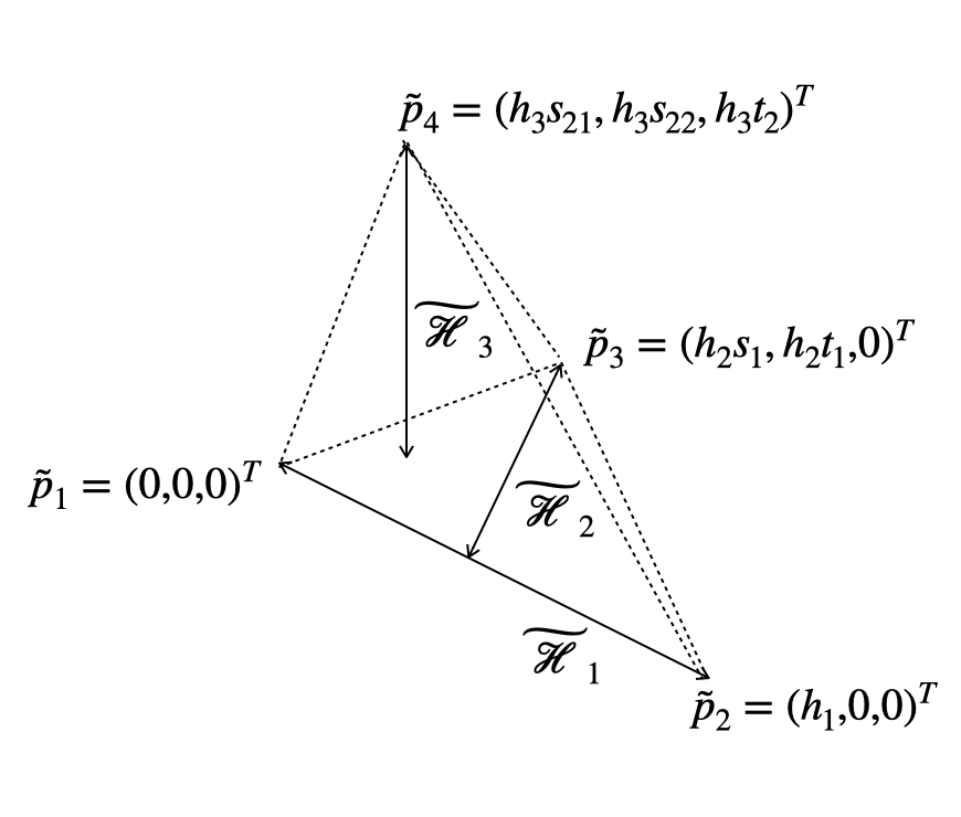
Figure 1: New parameters $\widetilde{\mathscr{H}}_{i}$, $i=1,2,3$

We defined the vectors ${r}_{n}\in\mathbb{R}^{d}$ and $n=1,\ldots,d$ as follows: If $d=2$,

$$\displaystyle{r}_{1}:=\frac{p_{2}-p_{1}}{|p_{2}-p_{1}|},\quad\tilde{r}_{2}:=\frac{p_{3}-p_{1}}{|p_{3}-p_{1}|},$$

and if $d=3$,

$${r}_{1}:=\frac{p_{2}-p_{1}}{|p_{2}-p_{1}|},\quad{r}_{3}:=\frac{p_{4}-p_{1}}{|p_{4}-p_{1}|},\quad\begin{cases}\displaystyle{r}_{2}:=\frac{p_{3}-p_{1}}{|p_{3}-p_{1}|},\quad\text{for case (i)},\\ \displaystyle{r}_{2}:=\frac{p_{3}-p_{2}}{|p_{3}-p_{2}|}\quad\text{for case (ii)}.\end{cases}$$

Furthermore, we define the vectors $\tilde{r}_{n}\in\mathbb{R}^{d}$ and $n=1,\ldots,d$ as follows. If $d=2$,

$$\displaystyle\tilde{r}_{1}:=(1,0)^{T},\quad\tilde{r}_{2}:=(s,t)^{T},$$

and if $d=3$,

$$\tilde{r}_{1}:=(1,0,0)^{T},\quad\tilde{r}_{3}:=(s_{21},s_{22},t_{2})^{T},\quad\begin{cases}\tilde{r}_{2}:=(s_{1},t_{1},0)^{T}\quad\text{for case (i)},\\ \tilde{r}_{2}:=(-s_{1},t_{1},0)^{T}\quad\text{for case (ii)}.\end{cases}$$

For a sufficiently smooth function $\varphi$ and vector function $v:=(v_{1},\ldots,v_{d})^{T}$, we define the directional derivative of $i\in\{1,\ldots,d\}$ as:

$$\displaystyle\frac{\partial\varphi}{\partial{r_{i}}} :=({r}_{i}\cdot\nabla_{x})\varphi=\sum_{i_{0}=1}^{d}({r}_{i})_{i_{0}}\frac{\partial\varphi}{\partial x_{i_{0}}},$$

$$\frac{\partial v}{\partial r_{i}} :=\left(\frac{\partial v_{1}}{\partial r_{i}},\ldots,\frac{\partial v_{d}}{\partial r_{i}}\right)^{T}=(({r}_{i}\cdot\nabla_{x})v_{1},\ldots,({r}_{i}\cdot\nabla_{x})v_{d})^{T}.$$

For a multi-index $\beta=(\beta_{1},\ldots,\beta_{d})\in\mathbb{N}_{0}^{d}$, we use the following notation.

$$\displaystyle\partial^{\beta}\varphi:=\frac{\partial^{|\beta|}\varphi}{\partial x_{1}^{\beta_{1}}\ldots\partial x_{d}^{\beta_{d}}},\quad\partial^{\beta}_{r}\varphi:=\frac{\partial^{|\beta|}\varphi}{\partial r_{1}^{\beta_{1}}\ldots\partial r_{d}^{\beta_{d}}}.$$

Note that $\partial^{\beta}\varphi\neq\partial^{\beta}_{r}\varphi$.

We proposed a new geometric parameter $H_{T}$ in IshKobTsu21a .

Definition 1

Parameter $H_{T}$ is defined as follows:

$$\displaystyle H_{T}:=\frac{\prod_{i=1}^{d}h_{i}}{|T|}h_{T}.$$

We introduce geometric conditions to obtain the optimal convergence rate of the anisotropic error estimates.

Assumption 2

A family of meshes $\{\mathbb{T}_{h}\}$ is semi-regular if there exists $\gamma_{0}\mathop{\textgreater}0$ such that

$$\displaystyle\frac{H_{T}}{h_{T}}\leq\gamma_{0}\quad\forall\mathbb{T}_{h}\in\{\mathbb{T}_{h}\},\quad\forall T\in\mathbb{T}_{h}.$$ (3.6)

Remark 1

We consider the good elements on the meshes in IshKobTsu23a . On anisotropic meshes, good elements may satisfy the following conditions:

($d=2$)

$h_{2}\approx h_{2}t$;

($d=3$)

$h_{2}\approx h_{2}t_{1}$ and $h_{3}\approx h_{3}t_{2}$.

Remark 2

The geometric condition in (3.6) is equivalent to the maximum angle condition ( (IshKobTsu23a, , Theorem 1)).

3.4 Main theorem

The $L^{2}$-orthogonal projection $\Pi_{\widehat{T}}^{0}:L^{1}(\widehat{T})\to\mathbb{P}^{0}(\widehat{T})$ is defined such that, for any $\hat{\varphi}\in L^{1}(\widehat{T})$,

$$\displaystyle\Pi_{\widehat{T}}^{0}\hat{\varphi}:=\frac{1}{|\widehat{T}|}\int_{\widehat{T}}\hat{\varphi}d\hat{x},$$

where $|\widehat{T}|$ is a measure of $\widehat{T}$; In setting ${\varphi}:=\hat{\varphi}\circ{\Phi}^{-1}$, the associated $L^{2}$-orthogonal projection $\Pi_{{T}}^{0}:L^{1}({T})\to\mathbb{P}^{0}({T})$ is defined as

$$\displaystyle\Pi_{{T}}^{0}{\varphi}:=\frac{1}{|{T}|}\int_{{T}}{\varphi}d{x},$$

where ${T}={\Phi}(\widehat{T})$, The following theorem provides an anisotropic error estimate for the projection $\Pi_{T}^{0}$.

Theorem 1

Let $p,q\in[1,\infty]$ such that $W^{1,p}(T)\hookrightarrow L^{q}(T)$. Then, for any $\hat{\varphi}\in W^{1,p}(\widehat{T})$ with ${\varphi}:=\hat{\varphi}\circ{\Phi}^{-1}$,

$$\displaystyle\|\Pi_{T}^{0}\varphi-\varphi\|_{L^{q}(T)}\leq c|T|^{\frac{1}{q}-\frac{1}{p}}\sum_{i=1}^{d}h_{i}\left\|\frac{\partial\varphi}{\partial r_{i}}\right\|_{L^{p}(T)}.$$ (3.7)

If Assumption 1 is imposed, then:

$$\displaystyle\|\Pi_{T}^{0}\varphi-\varphi\|_{L^{q}(T)}\leq c|T|^{\frac{1}{q}-\frac{1}{p}}\sum_{i=1}^{d}\widetilde{\mathscr{H}}_{i}\left\|\frac{\partial(\varphi\circ\Phi_{T})}{\partial\tilde{x}_{i}}\right\|_{L^{p}(\Phi_{T}^{-1}(T))}.$$ (3.8)

Proof

The standard scaling argument yields the following:

$$\displaystyle\|\Pi_{T}^{0}\varphi-\varphi\|_{L^{q}(T)}\leq c|\det({A})|^{\frac{1}{q}}\|\Pi_{\widehat{T}}^{0}\hat{\varphi}-\hat{\varphi}\|_{L^{q}(\widehat{T})}.$$ (3.9)

For any $\hat{\eta}\in\mathbb{P}^{0}$, we have that

$$\displaystyle\|\Pi_{\widehat{T}}^{0}\hat{\varphi}-\hat{\varphi}\|_{L^{q}(\widehat{T})} \leq\|\Pi_{\widehat{T}}^{0}(\hat{\varphi}-\hat{\eta})\|_{L^{q}(\widehat{T})}+\|\hat{\eta}-\hat{\varphi}\|_{L^{q}(\widehat{T})},$$ (3.10)

because $\Pi_{\widehat{T}}^{0}\hat{\eta}=\hat{\eta}$, Using Hölder’s inequality yields

$$\displaystyle\|\Pi_{\widehat{T}}^{0}(\hat{\varphi}-\hat{\eta})\|_{L^{q}(\widehat{T})} =|\widehat{T}|^{\frac{1}{q}}|\Pi_{\widehat{T}}^{0}(\hat{\varphi}-\hat{\eta})|\leq|\widehat{T}|^{\frac{1}{q}-1}\|\hat{\varphi}-\hat{\eta}\|_{L^{1}(\widehat{T})}$$

$$\leq|\widehat{T}|^{\frac{1}{q}-\frac{1}{p}}\|\hat{\varphi}-\hat{\eta}\|_{L^{p}(\widehat{T})}.$$ (3.11)

Based on (3.9), (3.10), (3.11), and the Sobolev embedding theorem, we have that

$$\displaystyle\|\Pi_{T}^{0}\varphi-\varphi\|_{L^{q}(T)}\leq C_{1}(\widehat{T})|\det({A})|^{\frac{1}{q}}\inf_{\hat{\eta}\in\mathbb{P}^{0}}\|\hat{\varphi}-\hat{\eta}\|_{W^{1,p}(\widehat{T})}.$$ (3.12)

From the Bramble–Hilbert lemma (refer to (BreSco08, , Lemma 4.3.8)), a constant $\hat{\eta}_{\beta}\in\mathbb{P}^{0}$ exists such that for any $\hat{\varphi}\in W^{1,p}(\widehat{T})$,

$$\displaystyle|\hat{\varphi}-\hat{\eta}_{\beta}|_{W^{s,p}(\widehat{T})}\leq C^{BH}(\widehat{T})|\hat{\varphi}|_{W^{1,p}(\widehat{T})},\quad s=0,1.$$ (3.13)

Using the inequality in (IshKobTsu23a, , Lemma 6) with $m=0$, we can estimate inequality (3.13) as

$$\displaystyle|\hat{\varphi}|_{W^{1,p}(\widehat{T})}\leq c|\det({{A}})|^{-\frac{1}{p}}\sum_{i=1}^{d}h_{i}\left\|\frac{\partial\varphi}{\partial r_{i}}\right\|_{L^{p}(T)}.$$ (3.14)

Using (3.12), (3.13), (3.14), and $|\det({{A}})|=\frac{|T|}{|\widehat{T}|}$, we can deduce the target inequality (3.7).

If Assumption 1 is imposed, using the inequality in (IshKobTsu23a, , Lemma 5) with $m=0$, we can estimate inequality (3.13) as follows:

$$\displaystyle|\hat{\varphi}|_{W^{1,p}(\widehat{T})}\leq c|\det({{A}})|^{-\frac{1}{p}}\sum_{i=1}^{d}\widetilde{\mathscr{H}}_{i}\left\|\frac{\partial\tilde{\varphi}}{\partial\tilde{x}_{i}}\right\|_{L^{p}(\widetilde{T})}.$$ (3.15)

Using (3.12), (3.13), (3.15), and $|\det({{A}})|=\frac{|T|}{|\widehat{T}|}$, we can deduce the target inequality (3.8) with $\tilde{\varphi}=\varphi\circ\Phi_{T}$ and $\widetilde{T}=\Phi_{T}^{-1}(T)$. ∎

Note 3

In inequality (3.8), obtaining the estimates in $T$ by specifically determining the matrix $A_{T}$ is possible. Let $p=q=2$. Recall that

$$\displaystyle\Phi_{T}:\widetilde{T}\ni\tilde{x}\mapsto x:={A}_{T}\tilde{x}+b_{T}\in T.$$

The space $\mathcal{C}^{1}(\widetilde{T})$ is dense in the space ${H}^{1}(\widetilde{T})$. For $\tilde{\varphi}\in\mathcal{C}^{2}(\widetilde{T})$ with $\varphi=\tilde{\varphi}\circ\Phi_{T}^{-1}$ and $1\leq i\leq d$, we have

$$\displaystyle\left|\frac{\partial\tilde{\varphi}}{\partial\tilde{x}_{i}}(\tilde{x})\right| =\left|\sum_{i_{1}^{(1)}=1}^{d}[A_{T}]_{i_{1}^{(1)}i}\frac{\partial\varphi}{\partial x_{i_{1}^{(1)}}}(x)\right|.$$

Let $d=2$. We define a rotation matrix $A_{T}$ as

$$\displaystyle A_{T}:=\begin{pmatrix}\cos\theta&-\sin\theta\\ \sin\theta&\cos\theta\end{pmatrix},$$

where $\theta$ denotes the angle. We then have

$$\displaystyle\left|\frac{\partial\tilde{\varphi}}{\partial\tilde{x}_{1}}(\tilde{x})\right| =\left|\cos\theta\frac{\partial\varphi}{\partial x_{1}}(x)+\sin\theta\frac{\partial\varphi}{\partial x_{2}}(x)\right|,$$

$$\left|\frac{\partial\tilde{\varphi}}{\partial\tilde{x}_{2}}(\tilde{x})\right| =\left|-\sin\theta\frac{\partial\varphi}{\partial x_{1}}(x)+\cos\theta\frac{\partial\varphi}{\partial x_{2}}(x)\right|.$$

If $|\sin\theta|\leq c\frac{\widetilde{\mathscr{H}}_{2}}{\widetilde{\mathscr{H}}_{1}}$ and $\widetilde{\mathscr{H}}_{2}\leq c\widetilde{\mathscr{H}}_{1}$, we can deduce

$$\displaystyle\left|\frac{\partial\tilde{\varphi}}{\partial\tilde{x}_{1}}(\tilde{x})\right| \leq\left|\frac{\partial\varphi}{\partial x_{1}}(x)\right|+c\frac{\widetilde{\mathscr{H}}_{2}}{\widetilde{\mathscr{H}}_{1}}\left|\frac{\partial\varphi}{\partial x_{2}}(x)\right|,$$

$$\left|\frac{\partial\tilde{\varphi}}{\partial\tilde{x}_{2}}(\tilde{x})\right| \leq c\left|\frac{\partial\varphi}{\partial x_{1}}(x)\right|+\left|\frac{\partial\varphi}{\partial x_{2}}(x)\right|.$$

As $|\det(A_{T})|=1$, it holds that for $i=1,2$,

$$\displaystyle\widetilde{\mathscr{H}}_{i}\left\|\frac{\partial\tilde{\varphi}}{\partial\tilde{x}_{i}}\right\|_{L^{2}(\widetilde{T})} \leq c\sum_{j=1}^{2}\widetilde{\mathscr{H}}_{j}\left\|\frac{\partial\varphi}{\partial x_{{j}}}\right\|_{L^{2}(T)},$$

which leads to

$$\displaystyle\|\Pi_{T}^{0}\varphi-\varphi\|_{L^{2}(T)}\leq c\sum_{j=1}^{2}\widetilde{\mathscr{H}}_{j}\left\|\frac{\partial\varphi}{\partial x_{{j}}}\right\|_{L^{2}(T)}.$$

As a special case, we set $\theta:=\frac{\pi}{2}$. We then have

$$\displaystyle\left|\frac{\partial\tilde{\varphi}}{\partial\tilde{x}_{1}}(\tilde{x})\right| =\left|\frac{\partial\varphi}{\partial x_{2}}(x)\right|,\quad\left|\frac{\partial\tilde{\varphi}}{\partial\tilde{x}_{2}}(\tilde{x})\right|=\left|\frac{\partial\varphi}{\partial x_{1}}(x)\right|.$$

As $|\det(A_{T})|=1$, it holds that

$$\displaystyle\left\|\frac{\partial\tilde{\varphi}}{\partial\tilde{x}_{i}}\right\|_{L^{2}(\widetilde{T})}\leq\left\|\frac{\partial\varphi}{\partial x_{{i+1}}}\right\|_{L^{2}(T)},$$

where indices $i$ and $i+1$ must be evaluated as in Modulo 2. We then have

$$\displaystyle\|\Pi_{T}^{0}\varphi-\varphi\|_{L^{2}(T)}\leq c\sum_{i=1}^{2}\widetilde{\mathscr{H}}_{i}\left\|\frac{\partial\varphi}{\partial x_{{i+1}}}\right\|_{L^{2}(T)}.$$

When $A_{T}$ is a mirror imaging matrix, similar estimates may hold. Furthermore, the same argument can be made in the case of $d=3$.

4 Interpolation error estimates of nonconforming finite element methods

We introduce the following theorem.

Theorem 2

Let $\alpha:=(\alpha_{1},\ldots,\alpha_{d})^{T}\in\mathbb{N}_{0}^{d}$ be a multi-index and $k\in\mathbb{N}$. Let $p\in[1,\infty)$ and $q\in[1,\infty)$ be such that

$$\displaystyle W^{1,p}({T})\hookrightarrow L^{q}({T}),$$ (4.1)

that is $1-\frac{d}{p}\geq-\frac{d}{q}$. We define an interpolation operator $I_{T}:W^{k,p}(T)\to\mathbb{P}^{k}(T)$ that satisfies:

$$\displaystyle\partial^{\alpha}(I_{{T}}{\varphi})=\Pi_{T}^{0}(\partial^{\alpha}\varphi)\quad\forall\varphi\in W^{k,p}(T)\quad{\forall\alpha:\ |\alpha|\leq k}.$$ (4.2)

Then, for any $\hat{\varphi}\in W^{k+1,p}(\widehat{T})$ with ${\varphi}:=\hat{\varphi}\circ{\Phi}^{-1}$ and any $\alpha$ with $|\alpha|\leq k$,

$$\displaystyle|I_{T}\varphi-\varphi|_{W^{k,q}({T})} \leq c|T|^{\frac{1}{q}-\frac{1}{p}}\sum_{i=1}^{d}h_{i}\left|\frac{\partial\varphi}{\partial r_{i}}\right|_{W^{k,p}(T)}.$$ (4.3)

If Assumption 1 is imposed, then:

$$\displaystyle|I_{T}\varphi-\varphi|_{W^{k,q}({T})} \leq c|T|^{\frac{1}{q}-\frac{1}{p}}\sum_{i=1}^{d}\widetilde{\mathscr{H}}_{i}\left|\frac{\partial(\varphi\circ\Phi_{T})}{\partial\tilde{x}_{i}}\right|_{W^{k,p}(\Phi_{T}^{-1}(T))}.$$ (4.4)

Proof

The error estimate of the $L^{2}$-orthogonal projection (3.7) yields

$$\displaystyle|I_{T}\varphi-\varphi|_{W^{k,q}({T})}^{q} =\sum_{|\alpha|=k}\left\|\partial^{\alpha}(I_{T}\varphi-\varphi)\right\|^{q}_{L^{q}(T)}$$

$$=\sum_{|\alpha|=k}\left\|\Pi_{T}^{0}(\partial^{\alpha}\varphi)-\partial^{\alpha}\varphi\right\|^{q}_{L^{q}(T)}$$

$$\leq c|T|^{\left(\frac{1}{q}-\frac{1}{p}\right)q}\sum_{|\alpha|=k}\sum_{i=1}^{d}h_{i}^{q}\left\|\partial^{\alpha}\frac{\partial\varphi}{\partial r_{i}}\right\|_{L^{p}(T)}^{q}.$$

Using the Jensen-type inequality (2.1), we obtain

$$\displaystyle|I_{T}\varphi-\varphi|_{W^{1,q}({T})} \leq c|T|^{\frac{1}{q}-\frac{1}{p}}\left(\sum_{i=k}^{d}h_{i}^{p}\sum_{|\alpha|=1}\left\|\partial^{\alpha}\frac{\partial\varphi}{\partial r_{i}}\right\|_{L^{p}(T)}^{p}\right)^{\frac{1}{p}}$$

$$\leq c|T|^{\frac{1}{q}-\frac{1}{p}}\sum_{i=1}^{d}h_{i}\left|\frac{\partial\varphi}{\partial r_{i}}\right|_{W^{k,p}(T)},$$

which is the target inequality in Eq. (4.3).

If Assumption 1 is imposed, then (3.8) yields

$$\displaystyle|I_{T}\varphi-\varphi|_{W^{k,q}({T})}^{q} \leq c|T|^{\left(\frac{1}{q}-\frac{1}{p}\right)q}\sum_{|\alpha|=k}\sum_{i=1}^{d}\widetilde{\mathscr{H}}_{i}^{q}\left\|\partial^{\alpha}\frac{\partial(\varphi\circ\Phi_{T})}{\partial\tilde{x}_{i}}\right\|_{L^{p}(\Phi_{T}^{-1}(T))}^{q}.$$

Using the Jensen-type inequality in (2.1), we obtained the target inequality in (4.4). ∎

Note 4

The operators that satisfy (4.2) exist; see Theorems 3 and 4.

4.1 Crouzeix–Raviart interpolation error estimate

Let ${F}_{i}$ and $1\leq i\leq d+1$ be the $(d-1)$-dimensional sub-simplex of ${T}$ opposite vertex ${p}_{i}$. The CR finite element on the reference element is defined by the triple $\{{T},{P},{\Sigma\}}$ as follows:

1. ${P}:=\mathbb{P}^{1}({T})$;

2. ${\Sigma}$ is a set $\{{\chi}_{i}\}_{1\leq i\leq N^{(d,1)}}$ of $N^{(d,1)}$ linear forms $\{{\chi}_{i}\}_{1\leq i\leq N^{(d,1)}}$ with its components such that, for any ${q}\in{P}$,

   $$\displaystyle{\chi}_{i}({q}):=\frac{1}{|{F}_{i}|}\int_{{F}_{i}}{q}d{s}\quad\forall i\in\{1,\ldots,d+1\}.$$ (4.5)

Using the barycentric coordinates $\{{\lambda}_{i}\}_{i=1}^{d+1}:\mathbb{R}^{d}\to\mathbb{R}$ on the reference element, the nodal basis functions associated with the degrees of freedom using (4.5) is defined as follows:

$$\displaystyle{\theta}_{i}({x}):=d\left(\frac{1}{d}-{\lambda}_{i}({x})\right)\quad\forall i\in\{1,\ldots,d+1\}.$$ (4.6)

Thus, ${\chi}_{i}({\theta}_{j})=\delta_{ij}$ for any $i,j\in\{1,\ldots,d+1\}$, The local operator ${I}_{{T}}^{CR}$ is defined as

$$\displaystyle I_{{T}}^{CR}:W^{1,1}({T})\ni{\varphi}\mapsto I_{{T}}^{CR}{\varphi}:=\sum_{i=1}^{d+1}\left(\frac{1}{|{F}_{i}|}\int_{{F}_{i}}{\varphi}d{s}\right){\theta}_{i}\in{P}.$$ (4.7)

We present anisotropic CR interpolation error estimates (see ApeNicSch01 ).

Theorem 3

Let $p\in[1,\infty)$ and $q\in[1,\infty)$ be such that (4.1) holds. Subsequently, for any ${\varphi}\in W^{2,p}({T})$,we have

$$\displaystyle|I_{T}^{CR}\varphi-\varphi|_{W^{1,q}({T})} \leq c|T|^{\frac{1}{q}-\frac{1}{p}}\sum_{i=1}^{d}h_{i}\left|\frac{\partial\varphi}{\partial r_{i}}\right|_{W^{1,p}(T)}.$$ (4.8)

If Assumption 1 is imposed, then:

$$\displaystyle|I_{T}^{CR}\varphi-\varphi|_{W^{1,q}({T})} \leq c|T|^{\frac{1}{q}-\frac{1}{p}}\sum_{i=1}^{d}\widetilde{\mathscr{H}}_{i}\left|\frac{\partial(\varphi\circ\Phi_{T})}{\partial\tilde{x}_{i}}\right|_{W^{1,p}(\Phi_{T}^{-1}(T))}.$$ (4.9)

Proof

Only CR interpolation satisfies the condition (4.2).

For ${\varphi}\in W^{2,p}({T})$, Green’s formula and the definition of the CR interpolation imply that because $I_{T}^{CR}\varphi\in\mathbb{P}^{1}$,

$$\displaystyle\frac{\partial}{\partial{x}_{j}}(I_{T}^{CR}\varphi) =\frac{1}{|T|}\int_{T}\frac{\partial}{\partial{x}_{j}}(I_{T}^{CR}\varphi)dx=\frac{1}{|T|}\sum_{i=1}^{d+1}n_{{T}}^{(j)}\int_{F_{i}}I_{T}^{CR}\varphi ds$$

$$=\frac{1}{|T|}\sum_{i=1}^{d+1}n_{{T}}^{(j)}\int_{F_{i}}\varphi ds=\frac{1}{|T|}\int_{T}\frac{\partial\varphi}{\partial{x}_{j}}dx=\Pi_{T}^{0}\left(\frac{\partial\varphi}{\partial{x}_{j}}\right)$$

for $j=1,\ldots,d$, where $n_{{T}}$ denotes the outer unit normal vector to $T$ and $n_{{T}}^{(j)}$ denotes the $j$th component of $n_{T}$. Therefore, from Theorem 2, the target inequalities (4.8) and (4.9) hold. ∎

4.2 Morley interpolation error estimate

The Morley FEM has not been defined uniquely. There are two versions: one defined in Mol68 , which is the original paper, and the other in ArnBre85 ; LasLea75 ; WanJin06 . In original Morley FEM, by normal derivatives on faces, the spans of the nodes are not preserved under push-forward. To overcome this difficulty, the mean value of the first normal derivative is used ArnBre85 ; LasLea75 ; WanJin06 . The original Morley interpolation error estimates are obtained using the modified Morley interpolation error estimates (see LasLea75 ). In this study, we use the Morley FEM introduced in WanJin06 .

Let ${F}_{i}$, $1\leq i\leq d+1$ be the $(d-1)$-dimensional subsimplex of ${T}$ without vertices ${p}_{i}$ and ${S}_{i,j}$, $1\leq i\mathop{\textless}j\leq d+1$ be the $(d-2)$-dimensional subsimplex of ${T}$ without vertices ${p}_{i}$ and ${p}_{j}$. The $d$-dimensional Morley finite element on the reference element is defined by the triple $\{{T},{P},{\Sigma\}}$ as

1. ${P}:=\mathbb{P}^{2}({T})$;

2. ${\Sigma}$ is a set $\{{\chi}_{i}\}_{1\leq i\leq N^{(d,2)}}$ of $N^{(d,2)}$ linear forms $\{{\chi}^{(1)}_{i,j}\}_{1\leq i\mathop{\textless}j\leq d+1}\cup\{{\chi}^{(2)}_{i}\}_{1\leq i\leq d+1}$ with its components such that, for any ${q}\in{P}$,

   $$\displaystyle{\chi}^{(1)}_{i,j}({q}) :=\frac{1}{|{S}_{i,j}|}\int_{{S}_{i,j}}{q}d{s},\quad 1\leq i\mathop{\textless}j\leq d+1,$$ (4.10a)

   $${\chi}^{(2)}_{i}({q}) :=\frac{1}{|{F}_{i}|}\int_{{F}_{i}}\frac{\partial{q}}{\partial{n}_{i}}d{s},\quad 1\leq i\leq d+1,$$ (4.10b)

   where $\frac{\partial}{\partial{n}_{i}}=n_{{T,i}}\cdot\nabla$, and $n_{{T,i}}$ is the unit outer normal to ${F}_{i}\subset\partial{T}$. For $d=2$, ${\chi}^{(1)}_{i,j}({q})$ is interpreted as

   $$\displaystyle{\chi}^{(1)}_{i,j}({q})={q}({p}_{k}),\quad k=1,2,3,\quad k\neq i,j.$$

For a Morley finite, ${\Sigma}$ is unisolvent (see (WanJin06, , Lemma 2)). The nodal basis functions associated with the degrees of freedom provided by (4.10) are defined as follows:

$$\displaystyle{\theta}_{i,j}^{(1)} :=1-(d-1)({\lambda}_{i}+{\lambda}_{j})+d(d-1){\lambda}_{i}{\lambda}_{j}$$

$$\quad-(d-1)(\nabla{\lambda}_{i})^{T}\nabla{\lambda}_{j}\sum_{k=i,j}\frac{{\lambda}_{k}(d{\lambda}_{k}-2)}{2|\nabla{\lambda}_{k}|_{E}^{2}},\quad 1\leq i\mathop{\textless}j\leq d+1,$$ (4.11a)

$${\theta}_{i}^{(2)} :=\frac{{\lambda}_{i}(d{\lambda}_{i}-2)}{2|\nabla{\lambda}_{i}|_{E}},\quad 1\leq i\leq d+1,$$ (4.11b)

where $|\nabla{\lambda}_{i}|_{E}$ denotes the Euclidean norm in $\mathbb{R}^{d}$. Subsequently, (WanJin06, , Theorem 1) proved that, for $1\leq i\mathop{\textless}j\leq d+1$,

$$\displaystyle{\chi}^{(1)}_{k,\ell}({\theta}_{i,j}^{(1)})=\delta_{ik}\delta_{j\ell},\quad 1\leq k\mathop{\textless}\ell\leq d+1,\quad{\chi}^{(2)}_{k}({\theta}_{i,j}^{(1)})=0,\quad 1\leq k\leq d+1,$$ (4.12)

and, for $1\leq i\leq d+1$,

$$\displaystyle{\chi}^{(1)}_{k,\ell}({\theta}^{(2)}_{i})=0,\quad 1\leq k\mathop{\textless}\ell\leq d+1,\quad{\chi}^{(2)}_{k}({\theta}^{(2)}_{i})=\delta_{ik},\quad 1\leq k\leq d+1.$$ (4.13)

The local interpolation operator ${I}_{{T}}^{M}$ is defined as

$$\displaystyle{I}_{{T}}^{M}:W^{2,1}({T})\ni{\varphi}\mapsto{I}_{{T}}^{M}{\varphi}\in{P},$$ (4.14)

with

$$\displaystyle{I}_{{T}}^{M}{\varphi}:=\sum_{1\leq i\mathop{\textless}j\leq d+1}{\chi}^{(1)}_{i,j}({\varphi}){\theta}_{i,j}^{(1)}+\sum_{1\leq i\leq d+1}{\chi}^{(2)}_{i}({\varphi}){\theta}_{i}^{(2)}.$$ (4.15)

Then, it holds that ${I}_{{T}}^{M}{q}={q}$ for any ${q}\in{P}$ and ${\varphi}\in W^{2,1}({T})$.

$$\displaystyle{\chi}^{(1)}_{i,j}({I}_{{T}}^{M}{\varphi}) ={\chi}^{(1)}_{i,j}({\varphi}),\quad 1\leq i\mathop{\textless}j\leq d+1,$$ (4.16a)

$${\chi}^{(2)}_{i}({I}_{{T}}^{M}{\varphi}) ={\chi}^{(2)}_{i}({\varphi}),\quad 1\leq i\leq d+1.$$ (4.16b)

The following lemma holds ((WanJin06, , Lemma 1)).

Lemma 1

Let $T\subset\mathbb{R}^{d}$ be a simplex. $n_{T,k}$ denotes the unit outer normal to the face $F_{k}$, $k=1,\ldots,d+1$ of $T$, $S_{1},\ldots,S_{d}$ are all $(d-2)$-dimensional subsimplexes of $F_{k}$. Let $v\in\mathcal{C}^{1}(T)$ be such that

$$\displaystyle\int_{S_{\ell}}v=0,\quad\int_{F_{k}}\frac{\partial v}{\partial n_{k}}=0,$$ (4.17)

for any $\ell=1,\ldots,d$ and $k=1,\ldots,d+1$. It then holds that

$$\displaystyle\int_{F_{k}}\frac{\partial v}{\partial x_{i}}=0,\quad i=1,\ldots,d,\quad k=1,\ldots,d+1.$$ (4.18)

Proof

Let $v\in\mathcal{C}^{1}(T)$. Let $\xi\in\mathbb{R}^{d}$ be a constant vector, and let $\tau:=\xi-(\xi\cdot n_{T,k})n_{T,k}$. We have

$$\displaystyle\tau\cdot n_{T,k} =\xi\cdot n_{T,k}-(\xi\cdot n_{T,k})n_{T,k}\cdot n_{T,k}=0,$$

that is, $\tau$ is the tangent vector of $F_{k}$. Subsequently, from (4.17) we obtain

$$\displaystyle\int_{F_{k}}(\xi\cdot\nabla)v=\int_{F_{k}}\frac{\partial v}{\partial\tau}+(\xi\cdot n_{T,k})\int_{F_{k}}\frac{\partial v}{\partial n_{k}}=\int_{F_{k}}\frac{\partial v}{\partial\tau}.$$

Let $d=2$. Let $p_{k1}$ and $p_{k2}$ be the endpoints of the edge $F_{k}$, that is, $F_{k}=\overline{p_{k1}p_{k2}}$. Subsequently, from (4.17) we obtain

$$\displaystyle\int_{F_{k}}\frac{\partial v}{\partial\tau} =\int_{s=0}^{s=|F_{k}|}\frac{dv}{ds}\left(\frac{|F_{k}|-s}{|F_{k}|}p_{k1}+\frac{s}{|F_{k}|}p_{k2}\right)=v(p_{k2})-v(p_{k1})=0.$$ (4.19)

Let $d=3$. Let $\zeta^{(\ell)}$ be the unit outer normal of $S_{\ell}$ for $\ell=1,2,3$, From (4.17), the Gauss–Green formula yields

$$\displaystyle\int_{F_{k}}\frac{\partial v}{\partial\tau} =\sum_{\ell=1}^{3}\tau\cdot\zeta^{(\ell)}\int_{S_{\ell}}v=0.$$ (4.20)

From (4.19) and (4.20), it holds that for $d=2,3$

$$\displaystyle\int_{F_{k}}(\xi\cdot\nabla)v=0.$$ (4.21)

Let $e_{1},\ldots,e_{d}\in\mathbb{R}^{d}$ be a canonical basis. By setting $\xi:=e_{i}$ in (4.21), we obtain the desired result in (4.18) under Assumption (4.17). ∎

The anisotropic Morley interpolation error estimate is expressed as

Theorem 4

Let $p\in[1,\infty)$ and $q\in[1,\infty)$ be such that (4.1) holds true. Subsequently, for any ${\varphi}\in W^{3,p}({T})\cap\mathcal{C}^{1}({T})$,we have

$$\displaystyle|I_{T}^{M}\varphi-\varphi|_{W^{2,q}({T})} \leq c|T|^{\frac{1}{q}-\frac{1}{p}}\sum_{i=1}^{d}h_{i}\left|\frac{\partial\varphi}{\partial r_{i}}\right|_{W^{2,p}(T)}.$$ (4.22)

If Assumption 1 is imposed, then:

$$\displaystyle|I_{T}^{M}\varphi-\varphi|_{W^{2,q}({T})} \leq c|T|^{\frac{1}{q}-\frac{1}{p}}\sum_{i=1}^{d}\widetilde{\mathscr{H}}_{i}\left|\frac{\partial(\varphi\circ\Phi_{T})}{\partial\tilde{x}_{i}}\right|_{W^{2,p}(\Phi_{T}^{-1}(T))}.$$ (4.23)

Proof

Only Morley interpolation satisfies the condition (4.2).

Let ${\varphi}\in W^{3,p}({T})\cap\mathcal{C}^{1}(T)$ and set $v:=I_{T}^{M}\varphi-\varphi$. Using the definition of the Morley interpolation operator (4.16), we obtain

$$\displaystyle\int_{{S}_{i,j}}{v}d{s}=0,\quad 1\leq i\mathop{\textless}j\leq d+1,\quad\int_{{F}_{i}}\frac{\partial v}{\partial n_{i}}ds=0,\quad 1\leq i\leq d+1.$$

Therefore, from Lemma 1, we have

$$\displaystyle\int_{F_{i}}\frac{\partial v}{\partial x_{k}}=0,\quad i=1,\ldots,d+1,\quad k=1,\ldots,d.$$ (4.24)

From Green’s formula and (4.24), it follows that, for $1\leq j,k\leq d$,

$$\displaystyle\int_{{T}}\frac{\partial^{2}v}{\partial{x}_{j}\partial{x}_{k}}d{x} =\sum_{i=1}^{d+1}n_{{T},j}\int_{{F}_{i}}\frac{\partial v}{\partial{x}_{k}}d{s}=0,$$

which leads to

$$\displaystyle\frac{\partial^{2}}{\partial{x}_{j}\partial{x}_{k}}(I_{{T}}^{M}{\varphi})=\frac{1}{|T|}\int_{T}\frac{\partial^{2}}{\partial{x}_{j}\partial{x}_{k}}(I_{{T}}^{M}{\varphi})dx=\frac{1}{|T|}\int_{T}\frac{\partial^{2}\varphi}{\partial{x}_{j}\partial{x}_{k}}dx=\Pi_{T}^{0}\left(\frac{\partial^{2}\varphi}{\partial{x}_{j}\partial{x}_{k}}\right),$$

because $\frac{\partial^{2}}{\partial{x}_{j}\partial{x}_{k}}(I_{{T}}^{M}{\varphi})\in\mathcal{P}^{0}(T)$, Therefore, by Theorem 2, the target inequalities (4.22) and (4.23) hold. ∎

5 Preliminaries for anisotropic error analysis

5.1 Useful relation for anisotropic error analysis

For any $T\in\mathbb{T}_{h}$, the local RT polynomial space is defined as

$$\displaystyle\mathbb{RT}^{0}(T):=\mathbb{P}^{0}(T)^{d}+x\mathbb{P}^{0}(T),\quad x\in\mathbb{R}^{d}.$$

The RT finite element space is defined as follows:

$$\displaystyle V^{RT^{0}}_{h} :=\{v_{h}\in L^{1}(\Omega)^{d}:\ v_{h}|_{T}\in RT^{0}(T),\ \forall T\in\mathbb{T}_{h},\ [\![v_{h}\cdot n]\!]_{F}=0,\ \forall F\in\mathcal{F}_{h}\}.$$

The discontinuous and CR finite element spaces are defined as

$$\displaystyle P_{dc,h}^{m} :=\left\{p_{h}\in L^{2}(\Omega);\ p_{h}|_{T}\in\mathbb{P}^{m}({T})\quad\forall T\in\mathbb{T}_{h}\right\},\quad m\in\mathbb{N}_{0},$$

$$V_{h0}^{CR} :=\biggl{\{}\varphi_{h}\in P_{dc,h}^{1}:\ \int_{F}[\![\varphi_{h}]\!]ds=0\ \forall F\in\mathcal{F}_{h}\biggr{\}}$$

and the Morley finite element space is as follows:

$$\displaystyle V_{h}^{M} :=\biggl{\{}\varphi_{h}\in P_{dc,h}^{2}:\ \int_{F}\biggl{[}\!\biggl{[}\frac{\partial\varphi_{h}}{\partial n}\biggr{]}\!\biggr{]}ds=0\ \forall F\in\mathcal{F}_{h}^{i},$$

the integral average of $$\varphi_{h} (d-2)$$ over each -dimensional

$$\hskip 19.91684pt\text{subsimplex of $T\in\mathbb{T}_{h}$ is continuous}\biggr{\}},$$

$$V_{h0}^{M} :=\left\{\varphi_{h}\in V_{h}^{M};\ \text{degrees of freedom of $\varphi_{h}$ in \eqref{Mor1} vanish on $\partial\Omega$}\right\}.$$

In particular, for $d=2$, the space $V_{h0}^{M}$ is described as

$$\displaystyle V_{h0}^{M} :=\biggl{\{}\varphi_{h}\in P_{dc,h}^{2}:\ \int_{F}\biggl{[}\!\biggl{[}\frac{\partial\varphi_{h}}{\partial n}\biggr{]}\!\biggr{]}ds=0\ \forall F\in\mathcal{F}_{h},$$

$$\hskip 19.91684pt\text{$\varphi_{h}$ is continuous at each vertex in $\Omega$, $\varphi_{h}(p)=0$, \ $p\in\partial\Omega$}\biggr{\}}.$$

The following relationship is crucial in the error analysis of nonconforming finite elements on anisotropic meshes and holds for isotropic meshes:

Lemma 2

For any $v_{h}\in V^{RT^{0}}_{h}$ or $\psi_{h}\in H_{0}^{1}(\Omega)+V_{h0}^{CR}$,we have

$$\displaystyle\sum_{T\in\mathbb{T}_{h}}\int_{T}(v_{h}\cdot\nabla)\psi_{h}dx+\sum_{T\in\mathbb{T}_{h}}\int_{T}\mathop{\mathrm{div}}v_{h}\psi_{h}dx=0,$$ (5.1)

For any $v_{h}\in V^{RT^{0}}_{h}$ or $\varphi_{h}\in V_{h0}^{M}$

$$\displaystyle\sum_{T\in\mathbb{T}_{h}}\int_{T}\left(v_{h}\cdot\nabla\right)\frac{\partial\varphi_{h}}{\partial x_{i}}dx+\sum_{T\in\mathbb{T}_{h}}\int_{T}\mathop{\mathrm{div}}v_{h}\frac{\partial\varphi_{h}}{\partial x_{i}}dx=0,\quad i=1,\ldots,d.$$ (5.2)

Proof

For any $v_{h}\in V_{h}^{RT^{0}}$ and $\psi_{h}\in H_{0}^{1}(\Omega)+V_{h0}^{CR}$, using Green’s formula and that $v_{h}\cdot n_{F}\in\mathbb{P}^{0}(F)$ for any $F\in\mathcal{F}_{h}$, we can derive

$$\sum_{T\in\mathbb{T}_{h}}\int_{T}(v_{h}\cdot\nabla)\psi_{h}dx+\sum_{T\in\mathbb{T}_{h}}\int_{T}\mathop{\mathrm{div}}v_{h}\psi_{h}dx$$

$$\quad=\sum_{T\in\mathbb{T}_{h}}\int_{\partial T}(v_{h}\cdot n_{T})\psi_{h}ds=\sum_{F\in\mathcal{F}_{h}}\int_{F}[\![(v_{h}\psi_{h})\cdot n_{F}]\!]ds$$

$$\quad=\sum_{F\in\mathcal{F}_{h}^{i}}\int_{F}\left([\![v_{h}\cdot n_{F}]\!]\{\!\{\psi_{h}\}\!\}+\{\!\{v_{h}\}\!\}\cdot n_{F}[\![\psi_{h}]\!]\right)ds$$

$$\quad\quad+\sum_{F\in\mathcal{F}_{h}^{\partial}}\int_{F}(v_{h}\cdot n_{F})\psi_{h}ds=0,$$

and are given by (5.1).

Let $\varphi_{h}\in V_{h0}^{M}$. Suppose that $F\in\mathcal{F}_{h}^{i}$ with $F=T_{\natural}\cap T_{\sharp}$, $T_{\natural},T_{\sharp}\in\mathbb{T}_{h}$. Let $S_{1},\ldots,S_{d}$ denote all $(d-2)$-dimensional subsimplexes of $F$. According to Lemma 1, because

$$\displaystyle\int_{S_{\ell}}[\![\varphi_{h}]\!]ds=0,\quad\ell\in\{1,\ldots,d\},\quad\int_{F}\biggl{[}\!\biggl{[}\frac{\partial\varphi_{h}}{\partial n}\biggr{]}\!\biggr{]}_{F}ds=0$$

it holds that

$$\displaystyle\int_{F}\biggl{[}\!\biggl{[}\frac{\partial\varphi_{h}}{\partial x_{i}}\biggr{]}\!\biggr{]}_{F}ds=0\quad\forall F\in\mathcal{F}_{h}^{i},\ i=1,\ldots,d.$$ (5.3)

Similarly, it holds that

$$\displaystyle\int_{F}\frac{\partial\varphi_{h}}{\partial x_{i}}ds=0\quad\forall F\in\mathcal{F}_{h}^{\partial},\ i=1,\ldots,d.$$ (5.4)

By using Green’s formulas (5.3), (5.4), and $v_{h}\cdot n_{F}\in\mathbb{P}^{0}(F)$ for any $F\in\mathcal{F}_{h}$, we can derive

$$\sum_{T\in\mathbb{T}_{h}}\int_{T}(v_{h}\cdot\nabla)\frac{\partial\varphi_{h}}{\partial x_{i}}dx+\sum_{T\in\mathbb{T}_{h}}\int_{T}\mathop{\mathrm{div}}v_{h}\frac{\partial\varphi_{h}}{\partial x_{i}}dx$$

$$\quad=\sum_{T\in\mathbb{T}_{h}}\int_{\partial T}(v_{h}\cdot n_{T})\frac{\partial\varphi_{h}}{\partial x_{i}}ds$$

$$\quad=\sum_{F\in\mathcal{F}_{h}^{i}}\int_{F}\left([\![v_{h}\cdot n_{F}]\!]\biggl{\{}\!\biggl{\{}\frac{\partial\varphi_{h}}{\partial x_{i}}\biggr{\}}\!\biggr{\}}_{F}+\{\!\{v_{h}\}\!\}\cdot n_{F}\biggl{[}\!\biggl{[}\frac{\partial\varphi_{h}}{\partial x_{i}}\biggr{]}\!\biggr{]}_{F}\right)ds$$

$$\quad\quad+\sum_{F\in\mathcal{F}_{h}^{\partial}}\int_{F}(v_{h}\cdot n_{F})\frac{\partial\varphi_{h}}{\partial x_{i}}ds=0,$$

and are given by (5.2): ∎

5.2 Error estimate of the RT finite element method

Error estimates of RT finite element interpolation on anisotropic meshes can be found in Acoetal11 ; AcoDur99 ; DurLom08 ; FarNicPaq01 ; Ish22b . Here, we introduce our version Ish22b using a new geometric parameter (Definition 1).

For $q\in\mathbb{RT}^{0}(T)$, the local degrees of freedom are defined as

$$\displaystyle{\chi}^{RT^{0}}_{T,i}({q}):=\int_{{F}_{i}}{q}\cdot n_{T,i}d{s},\quad F_{i}\subset\partial T,\quad\forall i\in\{1,\ldots,d+1\}.$$

When setting $\Sigma_{T}^{RT^{0}}:=\{{\chi}^{RT^{0}}_{T,i}\}_{1\leq i\leq d+1}$, the triple $\{T,\mathbb{RT}^{0}(T),\Sigma_{T}^{RT^{0}}\}$ is a finite element. The local shape functions are as follows.

$$\displaystyle\theta_{T,i}^{RT^{0}}(x):=\frac{\iota_{{F_{i}},{T}}}{d|T|}(x-p_{i})\quad\forall i\in\{1,\ldots,d+1\},$$

where $\iota_{{F_{i}},{T}}:=1$ if ${n}_{T,{i}}$ points outwards, and $-1$ otherwise (ErnGue21a, , Chapter 14).

Let $\mathcal{I}_{T}^{RT^{0}}:H^{1}(T)^{d}\to\mathbb{RT}^{0}(T)$ be the RT interpolation operator such that for any $v\in H^{1}(T)^{d}$,

$$\displaystyle\mathcal{I}_{T}^{RT^{0}}:H^{1}(T)^{d}\ni v\mapsto\mathcal{I}_{T}^{RT}v:=\sum_{i=1}^{d+1}\left(\int_{{F}_{i}}{v}\cdot n_{T,i}d{s}\right)\theta_{T,i}^{RT^{0}}\in\mathbb{RT}^{0}(T).$$

The Piola transformation $\Psi:L^{1}(\widehat{T})^{d}\to L^{1}({T})^{d}$ is defined as follows:

$$\displaystyle\Psi:L^{1}(\widehat{T})^{d} \to L^{1}({T})^{d}$$

$$\hat{v} \mapsto v(x):=\Psi_{T}\circ{\Psi}_{\widetilde{T}}(\hat{v})(x)=\frac{1}{\det(A)}A\hat{v}(\hat{x}),\quad A={A}_{T}{A}_{\widetilde{T}}$$

with the following two Piola transformations:

$$\displaystyle{\Psi}_{\widetilde{T}}:L^{1}(\widehat{T})^{d} \to L^{1}(\widetilde{T})^{d}$$

$$\hat{v} \mapsto\tilde{v}(\tilde{x}):={\Psi}_{\widetilde{T}}(\hat{v})(\tilde{x}):=\frac{1}{\det({A}_{\widetilde{T}})}{A}_{\widetilde{T}}\hat{v}(\hat{x}),$$

$${\Psi}_{T}:L^{1}(\widetilde{T})^{d} \to L^{1}({T})^{d}$$

$$\tilde{v} \mapsto{v}({x}):={\Psi}_{T}(\tilde{v})({x}):=\frac{1}{\det({A}_{T})}{A}_{T}\tilde{v}(\tilde{x}).$$

The following two theorems are divided into the elements of (Type i) and (Type ii) in Section 3.2.2 for $d=3$.

Theorem 5

Let $T$ be an element with conditions 1 and 2 which satisfy (Type i) in Section 3.2.2 when $d=3$. For any $\hat{v}\in H^{1}(\widehat{T})^{d}$, ${v}=({v}_{1},\ldots,{v}_{d})^{T}:={\Psi}\hat{v}$

$$\displaystyle\|\mathcal{I}_{T}^{RT^{0}}v-v\|_{L^{2}(T)^{d}} \leq c\left(\frac{H_{T}}{h_{T}}\sum_{i=1}^{d}h_{i}\left\|\frac{\partial v}{\partial r_{i}}\right\|_{L^{2}(T)^{d}}+h_{T}\|\mathop{\mathrm{div}}{v}\|_{L^{2}({T})}\right).$$ (5.5)

If Assumption 1 is imposed, then:

$$\displaystyle\|\mathcal{I}_{T}^{RT^{0}}v-v\|_{L^{2}(T)^{d}} \leq c\Biggl{(}\frac{H_{T}}{h_{T}}\sum_{i=1}^{d}\widetilde{\mathscr{H}}_{i}\left\|\frac{\partial(\Psi_{T}^{-1}v)}{\partial\tilde{x}_{i}}\right\|_{L^{2}(\Phi_{T}^{-1}(T))^{d}}$$

$$\hskip 56.9055pt+h_{T}\|\mathop{\mathrm{div}}{(\Psi_{T}^{-1}v)}\|_{L^{2}(\Phi_{T}^{-1}(T))}\Biggr{)}.$$ (5.6)

Proof

The proof can be found in (Ish22b, , Theorem 2). ∎

Theorem 6

Let $d=3$. Let $T$ be an element with Condition 2 that satisfies (Type ii) in Section 3.2.2. For any $\hat{v}\in H^{1}(\widehat{T})^{3}$, ${v}=({v}_{1},v_{2},{v}_{3})^{T}:={\Psi}\hat{v}$

$$\displaystyle\|\mathcal{I}_{T}^{RT^{0}}v-v\|_{L^{2}(T)^{3}} \leq c\frac{H_{T}}{h_{T}}\left(h_{T}\sum_{i=1}^{3}\left\|\frac{\partial v}{\partial r_{i}}\right\|_{L^{2}(T)^{3}}\right).$$ (5.7)

If Assumption 1 is imposed, then:

$$\displaystyle\|\mathcal{I}_{T}^{RT^{0}}v-v\|_{L^{2}(T)^{3}} \leq c\frac{H_{T}}{h_{T}}\Biggl{(}\sum_{i=1}^{3}\widetilde{\mathscr{H}}_{i}\left\|\frac{\partial(\Psi_{T}^{-1}v)}{\partial\tilde{x}_{i}}\right\|_{L^{2}(\Phi_{T}^{-1}(T))^{3}}$$

$$\hskip 56.9055pt+h_{T}\sum_{i=1}^{3}\left\|\frac{\partial(\Psi_{T}^{-1}v)}{\partial\tilde{r}_{i}}\right\|_{L^{2}(\Phi_{T}^{-1}(T))^{3}}\Biggr{)}.$$ (5.8)

Proof

The proof can be found in (Ish22b, , Theorem 3). ∎

Note 5

Let $d=3$. An anisotropic RT interpolation error estimate cannot be obtained for (Type ii) in Section 3.2.2. Therefore, we did not obtain the advantage of using anisotropic meshes.

We define the global RT interpolation $\mathcal{I}_{h}^{RT^{0}}:(V_{h0}^{CR})^{d}\cup H^{1}(\Omega)^{d}\to V^{RT^{0}}_{h}$ as follows:

$$\displaystyle(\mathcal{I}_{h}^{RT^{0}}v)|_{T}=\mathcal{I}_{T}^{RT^{0}}(v|_{T})\quad\forall T\in\mathbb{T}_{h},\quad\forall v\in(V_{h0}^{CR})^{d}\cup H^{1}(\Omega)^{d}.$$

Furthermore, we define the global interpolation $\Pi_{h}^{0}$ to space $P_{dc,h}^{0}$ as:

$$\displaystyle(\Pi_{h}^{0}\varphi)|_{T}:=\Pi_{T}^{0}(\varphi|_{T})\quad\forall T\in\mathbb{T}_{h},\quad\forall\varphi\in L^{2}(\Omega).$$

The following relationship holds between the RT interpolation $\mathcal{I}_{h}^{RT^{0}}$ and $L^{2}$-projection $\Pi_{h}^{0}$:

Lemma 3

It holds that

$$\displaystyle\mathop{\mathrm{div}}(\mathcal{I}_{T}^{RT^{0}}v)=\Pi_{T}^{0}(\mathop{\mathrm{div}}v)\quad\forall v\in H^{1}(T_{j})^{d}.$$ (5.9)

Incorporating (5.9), for any $v\in H^{1}(\Omega)^{d}$, it holds that

$$\displaystyle\mathop{\mathrm{div}}(\mathcal{I}_{h}^{RT^{0}}v)=\Pi_{h}^{0}(\mathop{\mathrm{div}}v).$$ (5.10)

Proof

The proof is provided in (ErnGue21a, , Lemma 16.2). ∎

5.3 Error estimates of the Lagrange finite element interpolation for $d=2$

We introduce anisotropic Lagrange finite-element interpolation error estimates for the analysis. (See IshKobTsu23a for detailed results.)

Let ${I}_{T}^{L}:\mathcal{C}(T)\to\mathbb{P}^{1}(T)$ be the Lagrange interpolation operator such that for any $\varphi\in\mathcal{C}(T)$,

$$\displaystyle{I}_{T}^{L}:\mathcal{C}(T)\ni\varphi\mapsto I_{T}^{L}\varphi:=\sum_{i=1}^{3}\varphi(p_{i})\theta_{T,i}^{L}\in\mathbb{P}^{1}(T),$$

where the local shape functions are

$$\displaystyle\theta_{T,i}^{L}(x):={\lambda}_{T,i}(x),\quad i\in\{1,2,3\}.$$

Theorem 7

For all $\hat{\varphi}\in H^{2}(\widehat{T})$ with ${\varphi}:=\hat{\varphi}\circ{\Phi}^{-1}$, we have

$$\displaystyle|{\varphi}-I_{{T}}^{L}{\varphi}|_{H^{m}({T})}\leq c\left(\frac{H_{T}}{h_{T}}\right)^{m}\sum_{|\varepsilon|=2-m}{h}^{\varepsilon}|\partial_{r}^{\varepsilon}\varphi|_{H^{m}(T)},\quad m=0,1.$$ (5.11)

Proof

The proof can be found in (IshKobTsu23a, , Corollary 1). ∎

The conforming finite element spaces are defined as

$$\displaystyle V^{L}_{h} :=\{v_{h}\in H^{1}(\Omega);v_{h}|_{T}\in\mathbb{P}^{1}(T),\ \forall T\in\mathbb{T}_{h}\},\quad V^{L}_{h0}:=V^{L}_{h}\cap H_{0}^{1}(\Omega).$$

We set $N:=\dim V^{L}_{h}$. The global interpolation operator is defined as follows:

$$\displaystyle I_{h}^{ML}:V_{h0}^{M}\cup H^{2}_{0}(\Omega)\ni\varphi_{h}\mapsto I_{h}^{ML}\varphi_{h}:=\sum_{i=1}^{N}\varphi_{h}(P_{i})\theta_{i}\in V^{L}_{h0}.$$

Let $\{\mathbb{T}_{h}\}$ be a family of conformal meshes with semiregular properties (Assumption 2). Subsequently, for all $\varphi_{h}\in V_{h0}^{M}$

$$\displaystyle|I_{h}^{ML}\varphi_{h}-\varphi_{h}|_{H^{1}(\mathbb{T}_{h})} \leq ch|\varphi_{h}|_{H^{2}(\mathbb{T}_{h})},$$ (5.12)

$$\|I_{h}^{ML}\varphi_{h}-\varphi_{h}\|_{L^{2}(\Omega)} \leq ch^{2}|\varphi_{h}|_{H^{2}(\mathbb{T}_{h})}.$$ (5.13)

6 Application to the fourth-order elliptic problem

Below, we use the interpolation error estimates in the $r_{i}$-coordinate system for the analysis.

6.1 Continuous problem

Let $\Omega\subset\mathbb{R}^{2}$ be the bounded polygonal domain. The fourth-order elliptic problem involves determining $\psi:\Omega\to\mathbb{R}$ such that:

$$\displaystyle\nu\varDelta^{2}\psi =g\quad\text{in $\Omega$},\quad\psi=\frac{\partial\psi}{\partial n}=0\quad\text{on $\partial\Omega$},$$ (6.1)

where $g:\Omega\to\mathbb{R}$ is a given function and $\nu$ is a real parameter with $0\mathop{\textless}\nu\leq 1$. We define the bilinear form $a_{1}:H^{2}(\Omega)\times H^{2}(\Omega)\to\mathbb{R}$ as follows:

$$\displaystyle a_{1}(\psi,\varphi):=\sum_{i=1}^{2}\int_{\Omega}\nabla\frac{\partial\psi}{\partial x_{i}}\cdot\nabla\frac{\partial\varphi}{\partial x_{i}}dx$$

for any $\psi,\varphi\in H^{2}(\Omega)$. The typical variational formulation of the fourth-order elliptical problem (6.1) is as follows. For any $g\in H^{-1}(\Omega)$, we determine $\psi\in H_{0}^{2}(\Omega)$ such that

$$\displaystyle\nu a_{1}(\psi,\varphi)=\int_{\Omega}g\varphi dx\quad\forall\varphi\in H_{0}^{2}(\Omega).$$ (6.2)

According to the Lax–Milgram theorem, a unique solution exists $\psi\in H^{2}_{0}(\Omega)$ of the problem (6.2). The proof is straightforward (see (Gri11, , pp. 301-302)).

The following theorem is known.

Theorem 8

For any $g\in H^{-1}(\Omega)$, there exists $\varepsilon\mathop{\textgreater}0$ such that $u\in H^{\frac{5}{2}+\varepsilon}(\Omega)$. Furthermore, if $\Omega$ is convex, then solution $u$ to problem (6.2) belongs to $H^{3}(\Omega)$. In other words, $\varDelta^{2}$ is an isomorphism between $H^{3}(\Omega)\cap H^{2}_{0}(\Omega)$ and $H^{-1}(\Omega)$.

Proof

The proofs are provided in (Gri92, , Corollaries 3.4.2, 3.4.3) and (Gri11, , Corollary 7.3.2.5). ∎

6.2 Modified Morley method for the fourth-order elliptic problem

For any $g\in L^{2}(\Omega)$, the typical Morley FEM for problem (6.2) involves determining $\psi_{h}\in V_{h0}^{M}$ such that

$$\displaystyle\nu a_{h1}(\psi_{h},\varphi_{h})=\int_{\Omega}g\varphi_{h}dx\quad\forall\varphi_{h}\in V_{h0}^{M},$$ (6.3)

where the bilinear form $a_{h1}:(H^{2}(\Omega)+V_{h0}^{M})\times(H^{2}(\Omega)+V_{h0}^{M})\to\mathbb{R}$ is:

$$\displaystyle a_{h1}(\psi_{h},\varphi_{h}):=\sum_{i=1}^{2}\sum_{T\in\mathbb{T}_{h}}\int_{T}\nabla\frac{\partial\psi_{h}}{\partial x_{i}}\cdot\nabla\frac{\partial\varphi_{h}}{\partial x_{i}}dx.$$

However, because $V_{h0}^{M}\not\subset H_{0}^{1}(\Omega)$, the typical Morley function in (6.3) cannot be applied to $g\in H^{-1}(\Omega)$. Hence, we consider the modified Morley finite element approximation problem of (6.2) proposed in ArnBre85 . The problem involves determining $\psi_{h}^{*}\in V_{h0}^{M}$ such that

$$\displaystyle\nu a_{h1}(\psi_{h}^{*},\varphi_{h})=\int_{\Omega}gI_{h}^{ML}\varphi_{h}dx\quad\forall\varphi_{h}\in V^{M}_{h0}$$ (6.4)

for any $g\in H^{-1}(\Omega)$, where $I_{h}^{ML}$ is the usual interpolant of the conforming linear finite element defined in Section 5.3.

6.3 Stability

Lemma 4

Let $\{\mathbb{T}_{h}\}$ be a family of conformal meshes with semiregular properties (Assumption 2). Let $T\in\mathbb{T}_{h}$ be an element of the condition 1. We assume that $\Omega$ is convex, and $h\leq 1$. Then, it holds that, for any $\varphi_{h}\in V_{h0}^{M}$,

$$\displaystyle|I_{h}^{ML}\varphi_{h}|_{H^{1}(\Omega)}\leq c|\varphi_{h}|_{H^{2}(\mathbb{T}_{h})}.$$ (6.5)

Proof

Let $\varphi_{h}\in V_{h0}^{M}$, We set $q:=-\varDelta I_{h}^{ML}\varphi_{h}\in H^{-1}(\Omega)$, The dual problem for the fourth-order elliptic problem is to determine $\eta\in H^{2}_{0}(\Omega)$ such that:

$$\displaystyle a_{1}(\varphi,\eta)=\langle q,\varphi\rangle\quad\forall\varphi\in H^{2}_{0}(\Omega).$$ (6.6)

Because $\Omega$ is convex, the solution $\eta$ is in $H^{3}(\Omega)$, and the following holds:

$$\displaystyle\|\eta\|_{H^{3}(\Omega)}\leq c\|q\|_{H^{-1}(\Omega)}.$$ (6.7)

Let $\mathscr{D}(\Omega)$ be a linear space of infinitely differentiable functions with a compact support on $\Omega$. Using the Gaussian–Green formula, we obtain

$$\displaystyle\langle q,\varphi\rangle=\langle-\varDelta I_{h}^{ML}\varphi_{h},\varphi\rangle=\int_{\Omega}\nabla I_{h}^{ML}\varphi_{h}\cdot\nabla\varphi dx\quad\forall\varphi\in\mathscr{D}(\Omega).$$ (6.8)

Because $\mathscr{D}(\Omega)$ is dense in $H_{0}^{1}(\Omega)$, Equation (6.8) is valid for any $\varphi\in H_{0}^{1}(\Omega)$. Then,

$$\displaystyle\|q\|_{H^{-1}(\Omega)} =\sup_{0\neq\varphi\in H_{0}^{1}(\Omega)}\frac{\langle q,\varphi\rangle}{|\varphi|_{H^{1}(\Omega)}}=\sup_{0\neq\varphi\in H_{0}^{1}(\Omega)}\frac{\int_{\Omega}\nabla I_{h}^{ML}\varphi_{h}\cdot\nabla\varphi dx}{|\varphi|_{H^{1}(\Omega)}}$$

$$\leq|I_{h}^{ML}\varphi_{h}|_{H^{1}(\Omega)}.$$ (6.9)

Moreover, using (6.6) and the Gauss–Green formula, it holds that, for any $\varphi\in\mathscr{D}(\Omega)$,

$$\displaystyle\langle q,\varphi\rangle =\sum_{i=1}^{2}\int_{\Omega}\nabla\frac{\partial\eta}{\partial x_{i}}\cdot\nabla\frac{\partial\varphi}{\partial x_{i}}dx=-\sum_{i=1}^{2}\int_{\Omega}\varDelta\frac{\partial\eta}{\partial x_{i}}\frac{\partial\varphi}{\partial x_{i}}dx.$$ (6.10)

Equality (6.10) is valid for any $\varphi\in H_{0}^{1}(\Omega)$, and by substituting $I_{h}^{ML}\varphi_{h}$ for $\varphi$ in (6.8) and (6.10) and using (5.2), we obtain for any $v_{h}\in V_{h}^{RT^{0}}$.

$$\displaystyle|I_{h}^{ML}\varphi_{h}|^{2}_{H^{1}(\Omega)} =\langle q,I_{h}^{ML}\varphi_{h}\rangle=-\sum_{i=1}^{2}\int_{\Omega}\varDelta\frac{\partial\eta}{\partial x_{i}}\frac{\partial(I_{h}^{ML}\varphi_{h})}{\partial x_{i}}dx$$

$$=-\sum_{T\in\mathbb{T}_{h}}\sum_{i=1}^{2}\int_{T}\varDelta\frac{\partial\eta}{\partial x_{i}}\frac{\partial\varphi_{h}}{\partial x_{i}}dx+\sum_{T\in\mathbb{T}_{h}}\sum_{i=1}^{2}\int_{T}\varDelta\frac{\partial\eta}{\partial x_{i}}\frac{\partial(\varphi_{h}-I_{h}^{ML}\varphi_{h})}{\partial x_{i}}dx$$

$$=\sum_{T\in\mathbb{T}_{h}}\sum_{i=1}^{2}\int_{T}\left(v_{h}-\nabla\frac{\partial\eta}{\partial x_{i}}\right)\cdot\nabla\frac{\partial\varphi_{h}}{\partial x_{i}}dx$$

$$\quad+\sum_{T\in\mathbb{T}_{h}}\sum_{i=1}^{2}\int_{T}\left(\mathop{\mathrm{div}}v_{h}-\varDelta\frac{\partial\eta}{\partial x_{i}}\right)\frac{\partial\varphi_{h}}{\partial x_{i}}dx$$

$$\quad+\sum_{T\in\mathbb{T}_{h}}\sum_{i=1}^{2}\int_{T}\varDelta\frac{\partial\eta}{\partial x_{i}}\frac{\partial(\varphi_{h}-I_{h}^{ML}\varphi_{h})}{\partial x_{i}}dx+\sum_{T\in\mathbb{T}_{h}}\sum_{i=1}^{2}\int_{T}\nabla\frac{\partial\eta}{\partial x_{i}}\cdot\nabla\frac{\partial\varphi_{h}}{\partial x_{i}}dx$$

$$=I_{1}+I_{2}+I_{3}+I_{4}.$$ (6.11)

We set $v_{h}:=I_{h}^{RT^{0}}\nabla\frac{\partial\eta}{\partial x_{i}}$. Using (5.5), (6.7), (6.9), Assumption 2, and the Jenssen inequality, we can obtain an estimate of the term $I_{1}$ such that

$$\displaystyle|I_{1}| \leq c\sum_{T\in\mathbb{T}_{h}}\sum_{i=1}^{2}\left\|I_{T}^{RT^{0}}\nabla\frac{\partial\eta}{\partial x_{i}}-\nabla\frac{\partial\eta}{\partial x_{i}}\right\|_{L^{2}(T)^{2}}|\varphi_{h}|_{H^{2}(T)}$$

$$\leq c\sum_{T\in\mathbb{T}_{h}}\sum_{i=1}^{2}\left(\sum_{j=1}^{2}h_{j}\left\|\frac{\partial}{\partial r_{j}}\nabla\frac{\partial\eta}{\partial x_{i}}\right\|_{L^{2}(T)^{2}}+h_{T}\left\|\varDelta\frac{\partial\eta}{\partial x_{i}}\right\|_{L^{2}({T})}\right)|\varphi_{h}|_{H^{2}(T)}$$

$$\leq c\sum_{T\in\mathbb{T}_{h}}\left(\sum_{j=1}^{2}h_{j}\left|\frac{\partial\eta}{\partial r_{j}}\right|_{H^{2}(T)}+h_{T}|\eta|_{H^{3}(T)}\right)|\varphi_{h}|_{H^{2}(T)}$$

$$\leq c\sum_{T\in\mathbb{T}_{h}}\sum_{j=1}^{2}h_{j}\left|\frac{\partial\eta}{\partial r_{j}}\right|_{H^{2}(T)}|\varphi_{h}|_{H^{2}(\mathbb{T}_{h})}+h|\eta|_{H^{3}(T)}|\varphi_{h}|_{H^{2}(\mathbb{T}_{h})}$$

$$\leq ch|\eta|_{H^{3}(\Omega)}|\varphi_{h}|_{H^{2}(\mathbb{T}_{h})}\leq ch|I_{h}^{ML}\varphi_{h}|_{H^{1}(\Omega)}|\varphi_{h}|_{H^{2}(\mathbb{T}_{h})}.$$ (6.12)

Because

$$\displaystyle\mathop{\mathrm{div}}I_{h}^{RT^{0}}\nabla\frac{\partial\eta}{\partial x_{i}}=\Pi_{h}^{0}\mathop{\mathrm{div}}\nabla\frac{\partial\eta}{\partial x_{i}}=\Pi_{h}^{0}\varDelta\frac{\partial\eta}{\partial x_{i}},$$

Using (3.7), (6.7), and (6.9), and the stability of the $L^{2}$projection, we estimate $I_{2}$ as

$$\displaystyle|I_{2}| =\left|\sum_{T\in\mathbb{T}_{h}}\sum_{i=1}^{2}\int_{T}\left(\Pi_{T}^{0}\varDelta\frac{\partial\eta}{\partial x_{i}}-\varDelta\frac{\partial\eta}{\partial x_{i}}\right)\left(\frac{\partial\varphi_{h}}{\partial x_{i}}-\Pi_{T}^{0}\frac{\partial\varphi_{h}}{\partial x_{i}}\right)dx\right|$$

$$\leq\sum_{T\in\mathbb{T}_{h}}\sum_{i=1}^{2}\left\|\Pi_{T}^{0}\varDelta\frac{\partial\eta}{\partial x_{i}}-\varDelta\frac{\partial\eta}{\partial x_{i}}\right\|_{L^{2}(T)}\left\|\frac{\partial\varphi_{h}}{\partial x_{i}}-\Pi_{T}^{0}\frac{\partial\varphi_{h}}{\partial x_{i}}\right\|_{L^{2}(T)}$$

$$\leq ch|\eta|_{H^{3}(\Omega)}|\varphi_{h}|_{H^{2}(\mathbb{T}_{h})}\leq ch|I_{h}^{ML}\varphi_{h}|_{H^{1}(\Omega)}|\varphi_{h}|_{H^{2}(\mathbb{T}_{h})}.$$ (6.13)

Using the estimates (5.12) and (6.7), the term $I_{3}$ is estimated as follows:

$$\displaystyle|I_{3}| \leq c\sum_{T\in\mathbb{T}_{h}}|\eta|_{H^{3}(T)}\sum_{i=1}^{2}\left\|\frac{\partial(I_{h}^{ML}\varphi_{h}-\varphi_{h})}{\partial x_{i}}\right\|_{L^{2}(T)}$$

$$\leq c|\eta|_{H^{3}(\Omega)}|I_{h}^{ML}\varphi_{h}-\varphi_{h}|_{H^{1}(\mathbb{T}_{h})}$$

$$\leq ch|\eta|_{H^{3}(\Omega)}|\varphi_{h}|_{H^{2}(\mathbb{T}_{h})}\leq ch|I_{h}^{ML}\varphi_{h}|_{H^{1}(\Omega)}|\varphi_{h}|_{H^{2}(\mathbb{T}_{h})}.$$ (6.14)

By substituting $\eta$ for $\varphi$ in (6.8) and (6.9), we obtain:

$$\displaystyle|\eta|^{2}_{H^{2}(\Omega)} \leq a(\eta,\eta)=\langle q,\eta\rangle\leq c\|q\|_{H^{-1}(\Omega)}|\eta|_{H^{1}(\Omega)}\leq c|I_{h}^{ML}\varphi_{h}|_{H^{1}(\Omega)}|\eta|_{H^{1}(\Omega)}.$$ (6.15)

Furthermore, using the Gauss–Green formula and Poincaré inequality, we obtain

$$\displaystyle|\eta|^{2}_{H^{1}(\Omega)} \leq\|\varDelta\eta\|_{L^{2}(\Omega)}\|\eta\|_{L^{2}(\Omega)}\leq c|\eta|_{H^{2}(\Omega)}|\eta|_{H^{1}(\Omega)}.$$ (6.16)

From (6.15) and (6.16), we have that

$$\displaystyle|\eta|_{H^{2}(\Omega)}\leq c|I_{h}^{ML}\varphi_{h}|_{H^{1}(\Omega)}.$$ (6.17)

Using (6.17), we estimate the term $I_{4}$ as

$$\displaystyle|I_{4}| \leq c|\eta|_{H^{2}(\Omega)}|\varphi_{h}|_{H^{2}(\mathbb{T}_{h})}\leq c|I_{h}^{ML}\varphi_{h}|_{H^{1}(\Omega)}|\varphi_{h}|_{H^{2}(\mathbb{T}_{h})}.$$ (6.18)

If $h\leq 1$, combining (6.11), (6.12), (6.13), (6.14), and (6.18) yields the target inequality (6.5). ∎

Theorem 9

Let $\{\mathbb{T}_{h}\}$ be a family of conformal meshes with semiregular properties (Assumption 2). Let $T\in\mathbb{T}_{h}$ be an element of the condition 1. We assume that $\Omega$ is convex, and $h\leq 1$. For any $g\in H^{-1}(\Omega)$, let $\psi_{h}^{*}\in V_{h0}^{M}$ be the solution to (6.4). Subsequently, it holds that

$$\displaystyle|\psi_{h}^{*}|_{H^{2}(\mathbb{T}_{h})}\leq c\|g\|_{H^{-1}(\Omega)}.$$ (6.19)

Proof

By substituting $\psi_{h}^{*}$ for $\varphi_{h}$ in (6.4), and using (6.7), we determine that the following holds:

$$\displaystyle|\psi_{h}^{*}|_{H^{2}(\mathbb{T}_{h})}^{2} \leq c\|g\|_{H^{-1}(\Omega)}|I_{h}^{ML}\psi_{h}^{*}|_{H^{1}(\Omega)}\leq c\|g\|_{H^{-1}(\Omega)}|\psi_{h}^{*}|_{H^{2}(\mathbb{T}_{h})},$$

which leads to the target inequality (6.19). ∎

Note 6

In Theorem 9, we have derived the stability estimate by imposing that $\Omega$ is convex. Because we used the regularity of the solution of the dual problem, the convexity can be not violated in our method.

6.4 Error analysis

The starting point for error analysis of the modified Morley FEM is the following inequality:

Lemma 5

Let $\psi\in H^{3}(\Omega)\cap H^{2}_{0}(\Omega)$ be the solution to the fourth-order elliptical problem in (6.2) with $\varDelta^{2}\psi\in H^{-1}(\Omega)$. Let $\psi_{h}^{*}\in V_{h0}^{M}$ be an approximate solution to the problem (6.4). It holds that

$$\displaystyle|\psi-\psi_{h}^{*}|_{H^{2}(\mathbb{T}_{h})} \leq c\inf_{v_{h}\in V_{h0}^{M}}|\psi-v_{h}|_{H^{2}(\mathbb{T}_{h})}$$

$$\quad+c\sup_{\varphi_{h}\in V_{h0}^{M}}\frac{\left|a_{h1}(\psi,\varphi_{h})-\int_{\Omega}\varDelta^{2}\psi I_{h}^{ML}\varphi_{h}dx\right|}{|\varphi_{h}|_{H^{2}(\mathbb{T}_{h})}}.$$ (6.20)

Proof

The proof is standard. ∎

The first term on the R.H.S. of inequality (6.20) is estimated as follows: Using the Morley interpolation error estimate (4.22) for any $\psi\in H^{3}(\Omega)$,

$$\displaystyle\inf_{v_{h}\in V_{h0}^{M}}|\psi-v_{h}|_{H^{2}(\mathbb{T}_{h})} \leq|\psi-I_{h}^{M}\psi|_{H^{2}(\mathbb{T}_{h})}\leq c\sum_{T\in\mathbb{T}_{h}}\sum_{i=1}^{2}h_{i}\left|\frac{\partial\psi}{\partial r_{i}}\right|_{H^{2}(T)}.$$ (6.21)

Here, we present the error estimate for the consistency term. It should be noted that $\psi\in H^{3}(\Omega)\cap H^{2}_{0}(\Omega)$ with $\varDelta^{2}\psi\in L^{2}(\Omega)$.

Lemma 6

Let $\{\mathbb{T}_{h}\}$ be a family of conformal meshes with semiregular properties (Assumption 2). Let $T\in\mathbb{T}_{h}$ be an element that satisfies Condition 1. Subsequently, there exists a positive constant $C$ independent of $h$, such that for any $\psi\in H^{3}(\Omega)\cap H^{2}_{0}(\Omega)$ with $\varDelta^{2}\psi\in L^{2}(\Omega)$ and $\varphi_{h}\in V_{h0}^{M}$,

$$\left|a_{h1}(\psi,\varphi_{h})-\int_{\Omega}\varDelta^{2}\psi I_{h}^{ML}\varphi_{h}dx\right|$$

$$\leq c\left(\sum_{T\in\mathbb{T}_{h}}\sum_{i=1}^{2}h_{i}\left|\frac{\partial\psi}{\partial r_{i}}\right|_{H^{2}(T)}\right)|\varphi_{h}|_{H^{2}(\mathbb{T}_{h})}+ch\|\nabla\varDelta\psi\|_{L^{2}(\Omega)^{2}}|\varphi_{h}|_{H^{2}(\mathbb{T}_{h})}.$$ (6.22)

Proof

Let $\psi\in H^{3}(\Omega)\cap H^{2}_{0}(\Omega)$ with $\varDelta^{2}\psi\in L^{2}(\Omega)$ and $\varphi_{h}\in V_{h0}^{M}$. Applying the Gaussian–Green formula and (5.2) yields, for any $v_{h,i}\in V_{h}^{RT^{0}}$, $i=1,2$,

$$a_{h1}(\psi,\varphi_{h})-\int_{\Omega}\varDelta^{2}\psi I_{h}^{ML}\varphi_{h}dx$$

$$=\sum_{T\in\mathbb{T}_{h}}\sum_{i=1}^{2}\int_{T}\left(\nabla\frac{\partial\psi}{\partial x_{i}}\cdot\nabla\frac{\partial\varphi_{h}}{\partial x_{i}}+\varDelta\frac{\partial\psi}{\partial x_{i}}\frac{\partial\varphi_{h}}{\partial x_{i}}+\varDelta\frac{\partial\psi}{\partial x_{i}}\frac{\partial(I_{h}^{ML}\varphi_{h}-\varphi_{h})}{\partial x_{i}}\right)dx$$

$$=\sum_{T\in\mathbb{T}_{h}}\sum_{i=1}^{2}\int_{T}\left(\nabla\frac{\partial\psi}{\partial x_{i}}-v_{h,i}\right)\cdot\nabla\frac{\partial\varphi_{h}}{\partial x_{i}}dx$$

$$+\sum_{T\in\mathbb{T}_{h}}\sum_{i=1}^{2}\int_{T}\left(\varDelta\frac{\partial\psi}{\partial x_{i}}-\mathop{\mathrm{div}}v_{h,i}\right)\frac{\partial\varphi_{h}}{\partial x_{i}}dx+\sum_{T\in\mathbb{T}_{h}}\sum_{i=1}^{2}\int_{T}\varDelta\frac{\partial\psi}{\partial x_{i}}\frac{\partial(I_{h}^{ML}\varphi_{h}-\varphi_{h})}{\partial x_{i}}dx$$

$$=:J_{1}+J_{2}+J_{3}.$$ (6.23)

Here, we use the first

$$\displaystyle-\int_{\Omega}\varDelta^{2}\psi I_{h}^{ML}\varphi_{h}dx =-\int_{\partial\Omega}(n\cdot\nabla)\varDelta\psi I_{h}^{ML}\varphi_{h}ds+\int_{\Omega}\nabla\varDelta\psi\cdot\nabla I_{h}^{ML}\varphi_{h}dx$$

$$=\int_{\Omega}\nabla\varDelta\psi\cdot\nabla I_{h}^{ML}\varphi_{h}dx,$$

because $I_{h}^{ML}\varphi_{h}\in H_{0}^{1}(\Omega)$,

In setting $v_{h,i}:=I_{h}^{RT^{0}}\nabla\frac{\partial\psi}{\partial x_{i}}$, the same method estimates terms $J_{1}$ and $J_{2}$ as terms $I_{1}$ and $I_{2}$ in Lemma 4. Subsequently,

$$\displaystyle|J_{1}| \leq c\sum_{T\in\mathbb{T}_{h}}\sum_{j=1}^{2}h_{j}\left|\frac{\partial\psi}{\partial r_{j}}\right|_{H^{2}(T)}|\varphi_{h}|_{H^{2}(\mathbb{T}_{h})}+ch\|\nabla\varDelta\psi\|_{L^{2}(\Omega)^{2}}|\varphi_{h}|_{H^{2}(\mathbb{T}_{h})},$$ (6.24)

$$|J_{2}| \leq ch\|\nabla\varDelta\psi\|_{L^{2}(\Omega)^{2}}|\varphi_{h}|_{H^{2}(\mathbb{T}_{h})}.$$ (6.25)

Using the estimate (5.12), term $J_{3}$ is estimated using the same method as that for term $I_{3}$ in lemma 4:

$$\displaystyle|J_{3}| \leq ch\|\nabla\varDelta\psi\|_{L^{2}(\Omega)^{2}}|\varphi_{h}|_{H^{2}(\mathbb{T}_{h})}.$$ (6.26)

Using (6.23), (6.24), (6.25), and (6.26), we can deduce the desired estimate (6.22). ∎

We presented an error estimate for a modified Morley FEM for a fourth-order elliptical problem.

Theorem 10

Let $\{\mathbb{T}_{h}\}$ be a family of conformal meshes with semiregular properties (Assumption 2). We assume all elements $T\in\mathbb{T}_{h}$ satisfy Condition 1. Let $\psi\in H^{3}(\Omega)\cap H^{2}_{0}(\Omega)$, where $\varDelta^{2}\psi\in L^{2}(\Omega)$ is the solution of the fourth-order elliptical problem in (6.2). Let $\psi_{h}^{*}\in V_{h0}^{M}$ be an approximate solution to the problem (6.4). Subsequently,

$$\displaystyle|\psi-\psi_{h}^{*}|_{H^{2}(\mathbb{T}_{h})} \leq c\sum_{T\in\mathbb{T}_{h}}\sum_{i=1}^{2}h_{i}\left|\frac{\partial\psi}{\partial r_{i}}\right|_{H^{2}(T)}+ch\|\nabla\varDelta\psi\|_{L^{2}(\Omega)^{2}}.$$ (6.27)

Proof

By combining (6.20), (6.21), and (6.22), we obtain target estimate (6.27). ∎

6.5 Usual Morley finite element method

From Theorem 10, we can deduce the error estimate for a typical Moley finite element problem (6.3).

Corollary 1

Let $\{\mathbb{T}_{h}\}$ be a family of conformal meshes with semiregular properties (Assumption 2). We assume all elements $T\in\mathbb{T}_{h}$ satisfy Condition 1. Let $\psi\in H^{3}(\Omega)\cap H^{2}_{0}(\Omega)$, where $\varDelta^{2}\psi\in L^{2}(\Omega)$ is the solution of the fourth-order elliptical problem in (6.2). Let $\psi_{h}\in V_{h0}^{M}$ be an approximate solution to the problem (6.3). Then,

$$\displaystyle|\psi-\psi_{h}|_{H^{2}(\mathbb{T}_{h})} \leq c\sum_{T\in\mathbb{T}_{h}}\sum_{i=1}^{2}h_{i}\left|\frac{\partial\psi}{\partial r_{i}}\right|_{H^{2}(T)}+ch\|\nabla\varDelta\psi\|_{L^{2}(\Omega)^{2}}+c\nu^{-1}h^{2}\|g\|_{L^{2}(\Omega)}.$$ (6.28)

Proof

The subtraction of (6.3) from (6.4) with $\varphi_{h}:=\psi_{h}^{*}-\psi_{h}$ and using (5.13) yields

$$\displaystyle\nu|\psi_{h}^{*}-\psi_{h}|^{2}_{H^{2}(\mathbb{T}_{h})} \leq\nu\|g\|_{L^{2}(\Omega)}\|I_{h}^{ML}(\psi_{h}^{*}-\psi_{h})-(\psi_{h}^{*}-\psi_{h})\|_{L^{2}(\Omega)}$$

$$\leq c\nu h^{2}\|g\|_{L^{2}(\Omega)}|\psi_{h}^{*}-\psi_{h}|_{H^{2}(\mathbb{T}_{h})},$$

which leads to

$$\displaystyle|\psi-\psi_{h}|_{H^{2}(\mathbb{T}_{h})} \leq|\psi-\psi_{h}^{*}|_{H^{2}(\mathbb{T}_{h})}+|\psi_{h}^{*}-\psi_{h}|_{H^{2}(\mathbb{T}_{h})}$$

$$\leq c\sum_{T\in\mathbb{T}_{h}}\sum_{i=1}^{2}h_{i}\left|\frac{\partial\psi}{\partial r_{i}}\right|_{H^{2}(T)}+ch\|\nabla\varDelta\psi\|_{L^{2}(\Omega)^{2}}+c\nu^{-1}h^{2}\|g\|_{L^{2}(\Omega)}.$$

∎

6.6 Three-dimensional case

When $d=3$, we considered the error estimate for the consistency term of a typical Morley FEM.
The starting point for the error analysis of the classical Morley FEM is as follows. Let $\psi\in H^{3}(\Omega)\cap H^{2}_{0}(\Omega)$ be the solution to the fourth-order elliptical problem (6.2) with $\varDelta^{2}\psi\in L^{2}(\Omega)$. Let $\psi_{h}\in V_{h0}^{M}$ be an approximate solution to the problem (6.3). It holds that

$$\displaystyle|\psi-\psi_{h}|_{H^{2}(\mathbb{T}_{h})} \leq c\inf_{v_{h}\in V_{h0}^{M}}|\psi-v_{h}|_{H^{2}(\mathbb{T}_{h})}$$

$$\quad+c\sup_{\varphi_{h}\in V_{h0}^{M}}\frac{\left|a_{h1}(\psi,\varphi_{h})-\int_{\Omega}\varDelta^{2}\psi\varphi_{h}dx\right|}{|\varphi_{h}|_{H^{2}(\mathbb{T}_{h})}}.$$ (6.29)

We used the RT interpolation error estimates for the error analysis of the consistency term (see Section 6.4). However, as stated in Note 5, we cannot obtain anisotropic RT interpolation error estimates for (Type ii) in Section 3.2.2. We use only case (Type i). Note that standard error analysis for (Type ii) can obtain the error estimates on isotropic meshes.
Let $\{\mathbb{T}_{h}\}$ be a family of conformal meshes with semiregular properties (Assumption 2). Let $T\in\mathbb{T}_{h}$ be an element satisfying Condition 2 which satisfy (type i) in Section 3.2.2. Let $w\in H^{1}_{0}(\Omega)$. We then have

$$\displaystyle a_{h1}(\psi,\varphi_{h})-\int_{\Omega}\varDelta^{2}\psi\varphi_{h}dx=a_{h1}(\psi,\varphi_{h})-\int_{\Omega}\varDelta^{2}\psi wdx+\int_{\Omega}\varDelta^{2}\psi(w-\varphi_{h})dx.$$ (6.30)

For the first and second terms on the R.H.S. of (6.30), the Gauss–Green formula and (5.2) yield:

$$a_{h1}(\psi,\varphi_{h})-\int_{\Omega}\varDelta^{2}\psi wdx$$

$$\quad=\sum_{T\in\mathbb{T}_{h}}\sum_{i=1}^{3}\int_{T}\left(\nabla\frac{\partial\psi}{\partial x_{i}}\cdot\nabla\frac{\partial\varphi_{h}}{\partial x_{i}}+\varDelta\frac{\partial\psi}{\partial x_{i}}\frac{\partial\varphi_{h}}{\partial x_{i}}+\varDelta\frac{\partial\psi}{\partial x_{i}}\frac{\partial(w-\varphi_{h})}{\partial x_{i}}\right)dx$$

$$\quad=\sum_{T\in\mathbb{T}_{h}}\sum_{i=1}^{3}\int_{T}\left(\nabla\frac{\partial\psi}{\partial x_{i}}-I_{h}^{RT^{0}}\nabla\frac{\partial\psi}{\partial x_{i}}\right)\cdot\nabla\frac{\partial\varphi_{h}}{\partial x_{i}}dx$$

$$\quad\quad+\sum_{T\in\mathbb{T}_{h}}\sum_{i=1}^{3}\int_{T}\left(\varDelta\frac{\partial\psi}{\partial x_{i}}-\mathop{\mathrm{div}}I_{h}^{RT^{0}}\nabla\frac{\partial\psi}{\partial x_{i}}\right)\frac{\partial\varphi_{h}}{\partial x_{i}}dx$$

$$\quad\quad+\sum_{T\in\mathbb{T}_{h}}\sum_{i=1}^{3}\int_{T}\varDelta\frac{\partial\psi}{\partial x_{i}}\frac{\partial(w-\varphi_{h})}{\partial x_{i}}dx.$$ (6.31)

From the first and second terms on the R.H.S. of (6.31), we can estimate the proof for (6.23). To complete the consistency error estimate, we must estimate the third term of the R.H.S. of (6.30) and the third term of the R.H.S. of (6.31); that is, we show that there exists $w\in H_{0}^{1}(\Omega)$ such that

$$\displaystyle\left\|\frac{\partial(w-\varphi_{h})}{\partial x_{i}}\right\|_{L^{2}(T)} \leq ch|\varphi_{h}|_{H^{2}(T)},\quad i\in\{1,2,3\},$$ (6.32)

$$\|w-\varphi_{h}\|_{L^{2}(T)} \leq ch^{2}|\varphi_{h}|_{H^{2}(T)}.$$ (6.33)

However, achieving (6.32) and (6.33) for anisotropic meshes may be difficult. Meanwhile, we can deduce the error estimate of the usual Morley finite element method on isotropic meshes, see (WanJin06, , Lemma 6).

7 Application to stream function formulation

7.1 Continuous problem

Let $\Omega\subset\mathbb{R}^{d}$ and $d\in\{2,3\}$ be the bounded polyhedral domains. The (scaled) Stokes equation is as follows: Determine $(u,p):\Omega\to\mathbb{R}^{d}\times\mathbb{R}$ such that

$$\displaystyle-\nu\varDelta u+\nabla p=f\quad\text{in $\Omega$},\quad\mathop{\mathrm{div}}u=0\quad\text{in $\Omega$},\quad u=0\quad\text{on $\partial\Omega$},$$ (7.1)

where $\nu$ is a nonnegative parameter and $f:\Omega\to\mathbb{R}^{d}$ is a given function. The variational formulation for the standard Stokes equation is as follows: For any $f\in L^{2}(\Omega)^{d}$, determine $(u,p)\in V:=H^{1}_{0}(\Omega)^{d}\times Q:=L^{2}_{0}(\Omega):=\left\{q\in L^{2}(\Omega);\ \int_{\Omega}qdx=0\right\}$ such that

$$\displaystyle\nu a_{2}(u,v)+b(v,p) =\int_{\Omega}f\cdot vdx\quad\forall v\in V,$$ (7.2a)

$$b(u,q) =0\quad\forall q\in Q,$$ (7.2b)

where the bilinear forms $a_{2}:H^{1}(\Omega)^{d}\times H^{1}(\Omega)^{d}\to\mathbb{R}$ and $b:H^{1}(\Omega)^{d}\times L^{2}(\Omega)\to\mathbb{R}$ are

$$a_{2}(u,v):=\sum_{i=1}^{d}\int_{\Omega}\nabla u_{i}\cdot\nabla v_{i}dx,\quad b(v,q):=-\int_{\Omega}\mathop{\mathrm{div}}vqdx.$$

for any $u,v\in H^{1}(\Omega)^{d}$ or $q\in L^{2}(\Omega)$. Using the space of weakly divergence-free functions, we obtain

$$\displaystyle V_{\mathop{\mathrm{div}}}:=\{v\in V;\ b(v,q)=0\ \forall q\in Q\}\subset V,$$

The problem associated with (7.2) is as follows. We determine $u\in V_{\mathop{\mathrm{div}}}$ such that

$$\displaystyle\nu a_{2}(u,v) =\int_{\Omega}f\cdot vdx\quad\forall v\in V_{\mathop{\mathrm{div}}}.$$ (7.3)

Theorem 11

If $d=2$ and $\Omega$ are convex, then the solution $(u,p)$ to the Stokes problem belongs to $u\in H^{2}(\Omega)^{2}$ and $p\in H^{1}(\Omega)$.

Proof

Reference KelOsb76 provides the proof. ∎

Let $d=2$ and assume that $\Omega$ is connected. As $u\in H^{1}_{0}(\Omega)^{2}$ is divergence-free, it holds that $u=\mathop{\mathrm{curl}}\psi$ for a unique stream function $\psi\in H^{2}_{0}(\Omega)$; see (GirRav86, , Section I.3.1). By setting $u:=\mathop{\mathrm{curl}}\psi$, Stokes problem  eqrefcont = 3is reduced to

$$\displaystyle\nu\varDelta^{2}\psi =g:=\mathop{\mathrm{rot}}f=\frac{\partial f_{2}}{\partial x_{1}}-\frac{\partial f_{1}}{\partial x_{2}}\quad\text{in $\Omega$},\quad\psi=\frac{\partial\psi}{\partial n}=0\quad\text{on $\partial\Omega$},$$ (7.4)

for any $f=(f_{1},f_{2})^{T}\in L^{2}(\Omega)^{2}$. This function is given in $H^{-1}(\Omega)$; see (GirRav86, , Section I.5.2) and (Gri11, , Section 7.3.3). Moreover, by setting $u:=\mathop{\mathrm{curl}}\psi$ and $v:=\mathop{\mathrm{curl}}\varphi$, the Stokes problem  eqrefcont = 5can be reduced to

$$\displaystyle\nu a_{1}(\psi,\varphi) =\int_{\Omega}f\cdot\mathop{\mathrm{curl}}\varphi dx\quad\forall\varphi\in H^{2}_{0}(\Omega).$$ (7.5)

7.2 Modified finite element method

The CR finite element space is defined as follows:

$$\displaystyle V_{h0}^{CR} :=\biggl{\{}\varphi_{h}\in P_{dc,h}^{1}:\ \int_{F}[\![\varphi_{h}]\!]ds=0\ \forall F\in\mathcal{F}_{h}\biggr{\}}.$$

We then define the Stokes pair $(V_{h},Q_{h})$ as

$$\displaystyle V_{h}:=(V_{h0}^{CR})^{d},\quad Q_{h}:=P_{dc,h}^{0}\cap L^{2}_{0}(\Omega).$$

Furthermore, we define $a_{h2}:(H^{1}(\Omega)^{d}+V_{h})\times H^{1}(\Omega)^{d}+V_{h})\to\mathbb{R}$ and $b_{h}:(V+V_{h})\times Q_{h}\to\mathbb{R}$, which are the discrete counterparts of the bilinear forms $a_{2}$ and $b$ as follows:

$$\displaystyle a_{h2}(u_{h},v_{h}) :=\sum_{i=1}^{d}\sum_{T\in\mathbb{T}_{h}}\int_{T}\nabla u_{h,i}\cdot\nabla v_{h,i}dx,$$

$$b_{h}(v_{h},q_{h}) :=-\sum_{T\in\mathbb{T}_{h}}\int_{T}\mathop{\mathrm{div}}v_{h}q_{h}dx.$$

The modified CR finite element approximation problem for the Stokes equation proposed in Lin14 is as follows. Determine $(u_{h}^{*},p_{h}^{*})\in V_{h}\times Q_{h}$ such that

$$\displaystyle\nu a_{h2}(u_{h}^{*},v_{h})+b_{h}(v_{h},p_{h}^{*}) =\int_{\Omega}f\cdot\mathcal{I}_{h}^{RT^{0}}v_{h}dx\quad\forall v_{h}\in V_{h},$$ (7.6a)

$$b_{h}(u_{h}^{*},q_{h}) =0\quad\forall q_{h}\in Q_{h},$$ (7.6b)

where the lifting operator $\mathcal{I}_{h}^{RT^{0}}$ is as defined in Section 5.2. We define a discrete weakly divergence-free subspace as

$$\displaystyle V_{h,\mathop{\mathrm{div}}}:=\{v_{h}\in V_{h}:\ b_{h}(v_{h},q_{h})=0\ \forall q_{h}\in Q_{h}\}.$$

Because $V_{h,\mathop{\mathrm{div}}}\not\subset V_{\mathop{\mathrm{div}}}$, space $V_{h,\mathop{\mathrm{div}}}$ is nonconforming in space $V_{\mathop{\mathrm{div}}}$. Subsequently, the problem associated with (7.6) is Determine $u_{h}^{*}\in V_{h,\mathop{\mathrm{div}}}$ such that:

$$\displaystyle\nu a_{h2}(u_{h}^{*},v_{h})=\int_{\Omega}f\cdot\mathcal{I}_{h}^{RT^{0}}v_{h}dx\quad\forall v_{h}\in V_{h,\mathop{\mathrm{div}}}.$$ (7.7)

7.3 Error analysis

Let $d=2$ and assume that $\Omega$ is connected. For any $\varphi_{h}\in V_{h0}^{M}$, we define the broken curl as

$$\displaystyle(\mathop{\mathrm{curl}_{h}}\varphi_{h})|_{T}=\mathop{\mathrm{curl}}\varphi_{h}|_{T}=\left(\frac{\partial\varphi_{h}}{\partial x_{2}},-\frac{\partial\varphi_{h}}{\partial x_{1}}\right)^{T}\Biggl{|}_{T}\quad\forall T\in\mathbb{T}_{h}.$$

The following theorem is known.

Theorem 12

The following holds:

$$\displaystyle V_{h,\mathop{\mathrm{div}}}=\mathop{\mathrm{curl}_{h}}V_{h0}^{M}.$$

Proof

Reference (FalMor90, , Theorem 4.1) provides the proof. ∎

The modified Morley FEM from the stream function formulation is as follows: For any $\psi_{h}^{**},\varphi_{h}\in V_{h0}^{M}$, substituting $u_{h}^{*}:=\mathop{\mathrm{curl}_{h}}\psi_{h}^{**}$ and $v_{h}:=\mathop{\mathrm{curl}_{h}}\varphi_{h}$ in the problem (7.7) yields the following problem: For any $f=(f_{1},f_{2})^{T}\in L^{2}(\Omega)^{2}$, determine $\psi_{h}^{**}\in V_{h0}^{M}$ such that

$$\displaystyle\nu a_{h1}(\psi_{h}^{**},\varphi_{h})=\int_{\Omega}f\cdot I_{h}^{RT^{0}}(\mathop{\mathrm{curl}_{h}}\varphi_{h})dx\quad\forall\varphi_{h}\in V_{h0}^{M}.$$ (7.8)

We considered a typical CR finite element method for the Stokes equation.

$$\displaystyle\nu a_{h1}(\psi_{h}^{**},\varphi_{h})=\int_{\Omega}f\cdot\mathop{\mathrm{curl}_{h}}\varphi_{h}dx\quad\forall\varphi_{h}\in V_{h0}^{M}.$$ (7.9)

For a sufficiently smooth function $f$, the R.H.S. of (7.9) cannot be replaced with

$$\displaystyle\sum_{T\in\mathbb{T}_{h}}\int_{T}\left(\frac{\partial f_{2}}{\partial x_{1}}-\frac{\partial f_{1}}{\partial x_{2}}\right)\varphi_{h}dx.$$

Because we have

$$\displaystyle\sum_{T\in\mathbb{T}_{h}}\int_{T}f\cdot\mathop{\mathrm{curl}_{h}}\varphi_{h}dx =\sum_{T\in\mathbb{T}_{h}}\int_{T}\left(\frac{\partial f_{2}}{\partial x_{1}}-\frac{\partial f_{1}}{\partial x_{2}}\right)\varphi_{h}dx$$

$$\quad+\sum_{T\in\mathbb{T}_{h}}\int_{\partial T}(f_{1}n_{T}^{(2)}-f_{2}n_{T}^{(1)})\varphi_{h}ds,$$ (7.10)

where $n_{T}:=(n_{T}^{(1)},n_{T}^{(2)})^{T}$ and the second term on the R.H.S. of (7.10) does not generally vanish.

The following inequality is the starting point for the error analysis of the modified Morley FEM (7.8):

Lemma 7

Let $\psi\in H^{3}(\Omega)\cap H^{2}_{0}(\Omega)$ be the solution to the fourth-order elliptical problem (7.5). Let $\psi_{h}^{**}\in V_{h0}^{M}$ be an approximate solution to (7.8). First, it holds that

$$\displaystyle|\psi-\psi_{h}^{**}|_{H^{2}(\mathbb{T}_{h})} \leq c\inf_{v_{h}\in V_{h0}^{M}}|\psi-v_{h}|_{H^{2}(\mathbb{T}_{h})}$$

$$\quad+c\nu^{-1}\sup_{\varphi_{h}\in V_{h0}^{M}}\frac{\left|\nu a_{h1}(\psi,\varphi_{h})-\int_{\Omega}f\cdot I_{h}^{RT^{0}}(\mathop{\mathrm{curl}_{h}}\varphi_{h})dx\right|}{|\varphi_{h}|_{H^{2}(\mathbb{T}_{h})}}.$$

Proof

The proof is standard. ∎

Let $(u,p)$ be the solution to the problem (7.1) with $f\in L^{2}(\Omega)^{2}$. Because

$$\displaystyle\int_{\Omega}\nabla p\cdot I_{h}^{RT^{0}}(\mathop{\mathrm{curl}_{h}}\varphi_{h})dx=0,\quad u=\mathop{\mathrm{curl}}\psi,\quad\psi\in H^{2}_{0}(\Omega),$$

and $\mathcal{I}_{h}^{RT^{0}}v_{h}$ is divergence-free on $T$ for any $v_{h}\in V_{h}$ (see (Joh16, , Lemma 4.134)), we have

$$\nu a_{h1}(\psi,\varphi_{h})-\int_{\Omega}f\cdot I_{h}^{RT^{0}}(\mathop{\mathrm{curl}_{h}}\varphi_{h})dx$$

$$\quad=\nu a_{h1}(\psi,\varphi_{h})+\int_{\Omega}\nu\varDelta\mathop{\mathrm{curl}}\psi\cdot I_{h}^{RT^{0}}(\mathop{\mathrm{curl}_{h}}\varphi_{h})dx.$$

We present only the error estimates for the consistency term.

Lemma 8

Let $\{\mathbb{T}_{h}\}$ be a family of conformal meshes with semiregular properties (Assumption 2). Let $T\in\mathbb{T}_{h}$ be an element that satisfies Condition 1. Subsequently, there exists a positive constant $C$ independent of $h$ such that for any $\psi\in H^{3}(\Omega)\cap H^{2}_{0}(\Omega)$ and $\varphi_{h}\in V_{h0}^{M}$,

$$\left|a_{h1}(\psi,\varphi_{h})+\int_{\Omega}\varDelta\mathop{\mathrm{curl}}\psi\cdot I_{h}^{RT^{0}}(\mathop{\mathrm{curl}_{h}}\varphi_{h})dx\right|$$

$$\quad\leq c\left(\sum_{T\in\mathbb{T}_{h}}\sum_{j=1}^{2}h_{j}\left|\frac{\partial\psi}{\partial r_{j}}\right|_{H^{2}(T)}\right)|\varphi_{h}|_{H^{2}(\mathbb{T}_{h})}+ch\left\|\varDelta\mathop{\mathrm{curl}}\psi\right\|_{L^{2}({\Omega})^{2}}|\varphi_{h}|_{H^{2}(\mathbb{T}_{h})}.$$ (7.11)

Proof

Let $\psi\in H^{3}(\Omega)\cap H^{2}_{0}(\Omega)$ and $\varphi_{h}\in V_{h0}^{M}$. By using the Gaussian–Green formula and (5.2), for any $v_{h,i}\in V_{h}^{RT^{0}}$ and $i=1,2$,

$$a_{h1}(\psi,\varphi_{h})+\int_{\Omega}\varDelta\mathop{\mathrm{curl}}\psi\cdot I_{h}^{RT^{0}}(\mathop{\mathrm{curl}_{h}}\varphi_{h})dx$$

$$\quad=\sum_{i=1}^{2}\sum_{T\in\mathbb{T}_{h}}\int_{T}\nabla\frac{\partial\psi}{\partial x_{i}}\cdot\nabla\frac{\partial\varphi_{h}}{\partial x_{i}}dx+\int_{\Omega}\varDelta\mathop{\mathrm{curl}}\psi\cdot\mathop{\mathrm{curl}_{h}}\varphi_{h}dx$$

$$\quad\quad+\int_{\Omega}\varDelta\mathop{\mathrm{curl}}\psi\cdot\left(I_{h}^{RT^{0}}(\mathop{\mathrm{curl}_{h}}\varphi_{h})-\mathop{\mathrm{curl}_{h}}\varphi_{h}\right)dx$$

$$\quad=\sum_{T\in\mathbb{T}_{h}}\sum_{i=1}^{2}\int_{T}\left(\nabla\frac{\partial\psi}{\partial x_{i}}-v_{h,i}\right)\cdot\nabla\frac{\partial\varphi_{h}}{\partial x_{i}}dx$$

$$\quad\quad+\sum_{T\in\mathbb{T}_{h}}\sum_{i=1}^{2}\int_{T}\left(\varDelta\frac{\partial\psi}{\partial x_{i}}-\mathop{\mathrm{div}}v_{h,i}\right)\frac{\partial\varphi_{h}}{\partial x_{i}}dx$$

$$\quad\quad+\int_{\Omega}\varDelta\mathop{\mathrm{curl}}\psi\cdot\left(I_{h}^{RT^{0}}(\mathop{\mathrm{curl}_{h}}\varphi_{h})-\mathop{\mathrm{curl}_{h}}\varphi_{h}\right)dx$$

$$\quad=K_{1}+K_{2}+K_{3}.$$ (7.12)

By setting $v_{h,i}:=I_{h}^{RT^{0}}\nabla\frac{\partial\psi}{\partial x_{i}}$ and using (2.1), we can estimate terms $K_{1}$ and $K_{2}$ using the same method as for terms $I_{1}$ and $I_{2}$ in Lemma 4 and $J_{1}$ and $J_{2}$ in Lemma 6.

$$\displaystyle|K_{1}| \leq c\sum_{T\in\mathbb{T}_{h}}\sum_{i=1}^{2}\left\|\nabla\frac{\partial\psi}{\partial x_{i}}-I_{T}^{RT^{0}}\nabla\frac{\partial\psi}{\partial x_{i}}\right\|_{L^{2}(T)^{2}}|\varphi_{h}|_{H^{2}(T)}$$

$$\leq c\sum_{T\in\mathbb{T}_{h}}\left(\sum_{i,j=1}^{2}h_{j}\left\|\frac{\partial^{2}\mathop{\mathrm{curl}}\psi}{\partial x_{i}\partial r_{j}}\right\|_{L^{2}(T)^{2}}+h_{T}\left\|\varDelta\mathop{\mathrm{curl}}\psi\right\|_{L^{2}({T})^{2}}\right)|\varphi_{h}|_{H^{2}(T)}$$

$$\leq c\sum_{T\in\mathbb{T}_{h}}\left(\sum_{j=1}^{2}h_{j}\left|\frac{\partial\psi}{\partial r_{j}}\right|_{H^{2}(T)}+h_{T}\left\|\varDelta\mathop{\mathrm{curl}}\psi\right\|_{L^{2}({T})^{2}}\right)|\varphi_{h}|_{H^{2}(T)}$$

$$\leq c\left\{\left(\sum_{T\in\mathbb{T}_{h}}\sum_{j=1}^{2}h_{j}\left|\frac{\partial\psi}{\partial r_{j}}\right|_{H^{2}(T)}\right)+h\left\|\varDelta\mathop{\mathrm{curl}}\psi\right\|_{L^{2}({\Omega})^{2}}\right\}|\varphi_{h}|_{H^{2}(\mathbb{T}_{h})},$$ (7.13)

and

$$\displaystyle|K_{2}| =\left|\sum_{T\in\mathbb{T}_{h}}\sum_{i=1}^{2}\int_{T}\left(\Pi_{T}^{0}\varDelta\frac{\partial\psi}{\partial x_{i}}-\varDelta\frac{\partial\psi}{\partial x_{i}}\right)\left(\frac{\partial\varphi_{h}}{\partial x_{i}}-\Pi_{T}^{0}\frac{\partial\varphi_{h}}{\partial x_{i}}\right)dx\right|$$

$$\leq\sum_{T\in\mathbb{T}_{h}}\sum_{i=1}^{2}\left\|\Pi_{T}^{0}\varDelta\frac{\partial\psi}{\partial x_{i}}-\varDelta\frac{\partial\psi}{\partial x_{i}}\right\|_{L^{2}(T)}\left\|\frac{\partial\varphi_{h}}{\partial x_{i}}-\Pi_{T}^{0}\frac{\partial\varphi_{h}}{\partial x_{i}}\right\|_{L^{2}(T)}$$

$$\leq ch\|\varDelta\mathop{\mathrm{curl}}\psi\|_{L^{2}(\Omega)^{2}}|\varphi_{h}|_{H^{2}(\mathbb{T}_{h})}.$$ (7.14)

Using (5.5), we estimate $K_{3}$:

$$\displaystyle|K_{3}| \leq ch\|\varDelta\mathop{\mathrm{curl}}\psi\|_{L^{2}(\Omega)^{2}}|\mathop{\mathrm{curl}}\varphi_{h}|_{H^{1}(\mathbb{T}_{h})}\leq ch\|\varDelta\mathop{\mathrm{curl}}\psi\|_{L^{2}(\Omega)^{2}}|\varphi_{h}|_{H^{2}(\mathbb{T}_{h})}.$$ (7.15)

The target inequality is proved based on (7.12), (7.13), (7.14), and (7.15). ∎

7.4 Conclusion

This study presented precise anisotropic interpolation error estimates for nonconforming FEMs. As applications, we demonstrated the anisotropic error estimates for the fourth-order elliptic problem (7.4) and stream function formulation (7.5). We denoted the solutions of the typical Morley, Arnord–Brezzi modified Morley, and the modified methods (7.8) from the stream function formulation by $\psi_{h}$, $\psi_{h}^{*}$, and $\psi_{h}^{**}$, respectively. For a convex polygonal domain, the following estimates hold.

$$\displaystyle|\psi-\psi_{h}|_{H^{2}(\mathbb{T}_{h})} \leq c\sum_{T\in\mathbb{T}_{h}}\sum_{i=1}^{2}h_{i}\left|\frac{\partial\psi}{\partial r_{i}}\right|_{H^{2}(T)}+ch\|\nabla\varDelta\psi\|_{L^{2}(\Omega)^{2}}+c\frac{h^{2}}{\nu}\left\|\mathop{\mathrm{rot}}f\right\|_{L^{2}(\Omega)},$$

$$|\psi-\psi_{h}^{*}|_{H^{2}(\mathbb{T}_{h})} \leq c\sum_{T\in\mathbb{T}_{h}}\sum_{i=1}^{2}h_{i}\left|\frac{\partial\psi}{\partial r_{i}}\right|_{H^{2}(T)}+ch\|\nabla\varDelta\psi\|_{L^{2}(\Omega)^{2}},$$

$$|\psi-\psi_{h}^{**}|_{H^{2}(\mathbb{T}_{h})} \leq c\sum_{T\in\mathbb{T}_{h}}\sum_{i=1}^{2}h_{i}\left|\frac{\partial\psi}{\partial r_{i}}\right|_{H^{2}(T)}+ch\left\|\varDelta u\right\|_{L^{2}({\Omega})^{2}}.$$

These are more delicate estimates than those of Falk and Morley FalMor90 , and they also apply without imposing the shape-regularity condition; however, a maximal angle condition is required. However, we impose the regularity assumption $\psi\in H^{3}(\Omega)\cap H^{2}_{0}(\Omega)$ with $\varDelta^{2}\psi\in L^{2}(\Omega)$ that is stronger than the original Arnord–Brezzi modified Morley method to prove the error estimate of the consistency term. The errors may be larger if the scheme is used without appropriate modifications and appropriate mesh partitions are not used. We aim to extend the proposed approach to numerical comparisons, fourth-order elliptic singular perturbation problems, and Navier-Stokes problems.

References

• (1) Acosta G., Apel Th, Durán R.G., Lombardi L.: Error estimates for Raviart–Thomas interpolating any order in anisotropic tetrahedra. Math. Comp. 80, 141-163 (2011)
• (2) Acosta, G., Durán, R.G.: The maximum angle condition for mixed and nonconforming elements: Application to the Stokes equations, SIAM J. Numer. Anal 37, 18-36 (1999)
• (3) Apel, Th.: Anisotropic finite elements: Local estimates and applications. Advances in Numerical Mathematics. Teubner, Stuttgart, (1999)
• (4) Apel, Th, Dobrowolski, M.: Anisotropic interpolation with applications to the finite element method. Computing 47, 277-293 (1992)
• (5) Apel, Th., Nicaise, S., Schöberl, J.: Crouzeix–Raviart type finite elements on anisotropic meshes. Numer. Math. 89, 193-223 (2001)
• (6) Arnold D.N., Brezzi F.: Mixed and nonconforming finite element methods: implementation, postprocessing and error estimates. RAIRO 19(1), 7-32 (1985)
• (7) Babuška, I., Aziz, A.K.: On the angle condition in the finite element method. SIAM J. Numer. Anal. 13, 214-226 (1976)
• (8) Brenner, S.C., Scott, L.R.: The Mathematical Theory of Finite Element Methods, Third Edition. Springer Verlag, New York (2008)
• (9) Ciarlet, P. G.: The Finite Element Method for Elliptic problems. SIAM, New York (2002)
• (10) Durán R.G., Lombardi L.: Error estimates for the Raviart–Thomas interpolation under the maximum angle condition. SIAM J. Numer. Anal. 46, 1442-1453 (2008)
• (11) Ern, A., Guermond, J.L.: Theory and Practice of Finite Elements. Springer Verlag, New York (2004)
• (12) Ern, A., Guermond, J.L.: Finite Elements I: Galerkin Approximation, Elliptic and Mixed PDEs. Springer Verlag, New York (2021)
• (13) Falk R.S., Morley M.E.: Equivalence of finite element methods for problems in elasticity. SIAM J Numer Anal 27:1486-1505 (1990)
• (14) Farhloul M., Nicaise S., Paquet L.: Some mixed finite Element Methods on Anisotropic Meshes. ESAIM: Mathematical Modelling and Numerical Analysis 35, 907-920 (2001)
• (15) Girault, V., Raviart, P.A.: Finite Element Methods for Navier-Stokes Equations. Springer-Verlag, (1986)
• (16) Grisvard, P.: Singularities in Boundary Value Problems. Masson, Springer (1992)
• (17) Grisvard, P.: Elliptic Problems in Nonsmooth Domains. SIAM, (2011)
• (18) Ishizaka, H.: Anisotropic Raviart–Thomas Interpolation Error Estimates Using a New Geometric Parameter. Calcolo 59 (4), (2022)
• (19) Ishizaka, H., Kobayashi, K., Tsuchiya, T.: General theory of interpolation error estimates on anisotropic meshes. Jpn. J. Ind. Appl. Math., 38 (1), 163-191 (2021)
• (20) Ishizaka, H., Kobayashi, K., Tsuchiya, T.: Anisotropic interpolation error estimates using a new geometric parameter. Jpn J Ind Appl Math 40 (1), 475-512 (2023)
• (21) John, V.: Finite element methods for incompressible flow problems. Springer Cham (2016)
• (22) Kellogg, R.B., Osborn, J.E.: A regularity result for the Stokes problem in a convex polygon. J Functional Analysis 21(4), 397-431 (1976)
• (23) K$\rm{\check{r}}$í$\rm{\check{z}}$ek, M.: On semiregular families of triangulations and linear interpolation. Appl. Math. Praha 36, 223-232 (1991)
• (24) K$\rm{\check{r}}$í$\rm{\check{z}}$ek, M.: On the maximum angle condition for linear tetrahedral elements. SIAM J. Numer. Anal. 29, 513-520 (1992)
• (25) Lascaux, P., Lesaint, P.: Some nonconforming finite element for the plate bending problem. RAIRO Anal Numer R-1, L9-53 (1975)
• (26) Linke, A.: On the role of the Helmholtz decomposition in mixed methods for incompressible flows and a new variational crime. Comput. Methods Anall. Mech. Engrg. 268, 782-800 (2014)
• (27) Mao, S., Nicaise, S., Shi, Z.-C.; Error estimates of Morley triangular element satisfying the maximal angle condition. International Journal of Numerical Analysis and Modeling 7 (4), 639-655 (2010)
• (28) Morley L.S.D.: The triangular equilibrium element in solving plate-bending problems. Aero Quart 19,149-169 (1968)
• (29) Nilssen, T.K., Tai, X-C, Winther, R.: A robust nonconforming $H^{2}$-element. Math Comp 70, 489-501 (2001)
• (30) Rannacher, R.: Finite element approximation of supported plates and the Babuška paradox. ZAMM 59, 73-76 (1979)
• (31) Rannacher, R.: On Nonconforming and Mixed Finite Elements for the Plate Bending Problem. RAIRO Model. Math Anal Numer 13:369-387 (1979)
• (32) Raviart, P. A., Thomas, J.-M.: A mixed finite element method for second order elliptic problems, in Mathematical Aspects of the Finite Element Method, I. Galligani, E. Magenes, eds., Lectures Notes in Math. 606, Springer Verlag, (1977)
• (33) Sohr, H.: The Navier-Stokes equations: An elementary functional analytic approach. Birkh$\rm{\ddot{a}}$user, Boston, Basel, Berlin, (2001)
• (34) Ming, W., Xu, J.: The Morley element for fourth order elliptic equations in any dimensions. Numer. Math. 103, 155-169 (2006)
• (35) Ming, W., Xu, J., Hu, Y.: Modified Morley element method for a fourth-order elliptic singular perturbation problem. J Comp Math 24(2), 113-120 (2006)