Search to Capture Long-range Dependency with Stacking GNNs for Graph Classification

Abstract.

In recent years, Graph Neural Networks (GNNs) have been popular in the graph classification task. Currently, shallow GNNs are more common due to the well-known over-smoothing problem facing deeper GNNs. However, they are sub-optimal without utilizing the information from distant nodes, i.e., the long-range dependencies. The mainstream methods in the graph classification task can extract the long-range dependencies either by designing the pooling operations or incorporating the higher-order neighbors, while they have evident drawbacks by modifying the original graph structure, which may result in information loss in graph structure learning. In this paper, by justifying the smaller influence of the over-smoothing problem in the graph classification task, we evoke the importance of stacking-based GNNs and then employ them to capture the long-range dependencies without modifying the original graph structure. To achieve this, two design needs are given for stacking-based GNNs, i.e., sufficient model depth and adaptive skip-connection schemes. By transforming the two design needs into designing data-specific inter-layer connections, we propose a novel approach with the help of neural architecture search (NAS), which is dubbed LRGNN (Long-Range Graph Neural Networks). Extensive experiments on five datasets show that the proposed LRGNN can achieve the best performance, and obtained data-specific GNNs with different depth and skip-connection schemes, which can better capture the long-range dependencies.

1. Introduction

In recent years, Graph Neural Networks (GNNs) have been the state-of-the-art (SOTA) method on graph classification (Zhang et al., 2018; Wang et al., 2021b), a popular task which can be applied into various domains, e.g., chemistry (Gilmer et al., 2017), bioinformatics (Ying et al., 2018; Wang et al., 2022d), text (Zhang et al., 2020) and social networks (Xu et al., 2019; Wang et al., 2021c; Yoo et al., 2022). In general, they encode the graph structure to learn node embeddings with the help of the message-passing scheme (Gilmer et al., 2017), i.e., aggregating messages from the connected nodes. Then, the graph representation vector can be generated with one readout operation, e.g., take the mean or summation of all node embeddings. In the literature, two- or three-layer GNNs are widely used since the performance decreases as the network goes deeper (Li et al., 2018). However, it limits the ability of GNNs to capture the long-range dependencies, i.e., incorporate information from long-distant neighbors (Lukovnikov and Fischer, 2021), which may be useful in the graph classification task (Jain et al., 2021; Dwivedi et al., 2022).

For the graph classification task, the majority of methods focus on designing the pooling operations to extract the hierarchical information in the graph (Lee et al., 2019; Ying et al., 2018). We review the literature from the perspective of long-range dependencies, and then observe that not all pooling operations are helpful in extracting the long-range dependencies. The grouping-based pooling operations (Ying et al., 2018; Bianchi et al., 2020; Yuan and Ji, 2020) group nodes into clusters and then re-design the edges between these clusters. These newly added edges may shorten the distance between node pairs, and then faster the feature propagation in the graph. On the contrary, the selection-based ones (Lee et al., 2019; Gao and Ji, 2019) construct the coarse graph by removing the low-ranked nodes and edges connected with them, which means the distance between nodes will not be shortened and are not helpful in incorporating the long-distant neighbors. Apart from pooling operations, several methods tend to incorporate the higher-order neighbors directly. For example, GraphTrans (Jain et al., 2021) adopts the transformer module which allows the interactions between all node pairs. Similarly, (Pham et al., 2017) provides one virtual node which connected with all nodes, and (Alon and Yahav, 2021) designs one fully adjacent (FA) aggregation layer in which all nodes are connected directly.

Despite the popularity of these methods in graph classification, they are deficient when capturing long-range dependencies on graphs. The aforementioned methods update the graph structure and may result in information loss in graph structure learning, either by generating the coarse graph or connecting to higher-order neighbors. Considering this, we revisit the stacking-based GNNs, which is a direct approach to obtaining the long-range dependencies while keeping the graph structures unchanged. In general, scaling the model depth is the most common way to improve the model performance (Tan and Le, 2019; Krizhevsky et al., 2012; Simonyan and Zisserman, 2014; He et al., 2016). and deeper stacking-based GNNs further bring the larger receptive field to incorporate the longer-distant neighbors. Nevertheless, the major concern to utilize the deeper GNNs is the over-smoothing problem (Li et al., 2018; Xu et al., 2018), i.e., the connected nodes tend to have similar features as the network goes deeper, which results in a performance drop in the node classification task. Yet, in this paper, we justify the smaller influence of this problem on the graph classification task compared with the node classification task both in theoretical analysis and experimental results. Therefore, designing stacking-based GNNs is indeed a feasible solution to capture the long-range dependencies.

Motivated by this, we propose a novel method LRGNN (Long-Range Graph Neural Networks), and employ the stacking-based GNNs to capture the long-range dependencies in graphs. There are two aspects that will affect the utilization of the long-distant neighbors: (a) sufficient model depth is required to incorporate the longer-distant neighbors; (b) adaptive skip-connection schemes are required considering the information mixing from different ranges of neighbors. The former is correlated with the inter-layer connections between the consecutive layers while the latter one related to the inconsecutive layers. Therefore, designing effective stacking-based GNNs to capture the long-range dependencies can be achieved by designing the inter-layer connections adaptively. We adopt the widely used neural architecture search (NAS) methods to achieve this.

To be specific, we provide one framework to design the inter-layer connections, which contains a set of learnable connections in the directed acyclic graphs (DAG). Two candidate choices are provided to represent the “used” and “unused” states in learnable connections, and then designing the inter-layer connections is transformed into deciding which choice should be adopted in each learnable connection. Then, the search space of LRGNN can be constructed based on the combinations of those connection choices, while the search space size is growing exponentially as the network goes deeper. Considering the search efficiency, we further provide one cell-based framework that only enables the connection designs in each cell, on top of which two variants LRGNN-Diverse and LRGNN-Repeat can be constructed. The differentiable search algorithm is adopted in this paper to enable the adaptive architecture design. In the experiments, we first evaluate the rationality of LRGNN by showing the higher performance achieved with sufficient model depth and various skip-connection schemes. Then, the extensive experimental results demonstrate that the proposed LRGNN can achieve the SOTA performance by designing GNNs with the inter-layer connections adaptively, on top of which the effectiveness of the proposed method can be verified.

To summarize, our contributions are as follows:

• We evoke the importance of stacking-based GNNs in extracting the long-range dependencies, and verify the smaller influence of the over-smoothing problem on the graph classification, on top of which two design needs are provided for designing stacking-based GNNs , i.e., the sufficient GNN depth and adaptive skip-connection schemes.

• To meet these two design needs, we firstly unify them into designing the inter-layer connections in stacking-based GNNs, and then achieve this with the help of NAS.

• We conduct extensive experiments on five datasets from different domains, and the proposed LRGNN achieves the SOTA performance by designing GNNs with sufficient model depth and adaptive skip-connection schemes.

Notations. We represent a graph as $\mathcal{G}=(\mathcal{V},\mathcal{E})$,where $\mathcal{V}$ and $\mathcal{E}$ represent the node and edge sets. $\textbf{A}\in\mathbb{R}^{|\mathcal{V}|\times|\mathcal{V}|}$ is the adjacency matrix of this graph where $|\mathcal{V}|$ is the node number. $\mathcal{N}(u)$ is the neighbors of node $u$. $\textbf{H}\in\mathbb{R}^{|\mathcal{V}|\times d}$ is the node feature matrix and $d$ is the feature dimension, and $\textbf{h}_{u}$ is the feature representation of node $u$.

2. Related Work: Graph neural network (GNN)

GNNs have advantages in encoding the graph structure information with the help of the message-passing scheme (Gilmer et al., 2017), i.e., aggregating the messages from connected nodes. It can be represented as $\textbf{h}_{v}=\textbf{W}(\textbf{h}_{v},\text{AGGR}\{\textbf{h}_{u},u\in\mathcal{N}(v)\})$, where W is the learnable parameter, AGGR is the aggregation function used in this aggregation operation. Diverse aggregation operations are proposed and widely used in graph representation learning (Kipf and Welling, 2016; Hamilton et al., 2017; Veličković et al., 2018; Chen et al., 2020). Based on these aggregation operations, one GNN can be constructed by stacking these aggregation operations.

2.1. Long-range Dependency Extraction in Graph Classification

In the graph classification task, existing literature can be grouped into three categories according to their methods in extracting the long-range dependencies, i.e., designing pooling operations, incorporating the higher-order neighbors, and stacking GNN layers.

2.1.1. Designing pooling operations

Pooling operations are widely used in the graph classification task, and they aim to generate one coarse graph to extract the hierarchical information. They can be classified into two groups, i.e., the selection-based ones and the grouping-based ones. The selection-based methods (Lee et al., 2019; Gao and Ji, 2019) focus on evaluating the node importance. The top-ranked nodes are preserved, and then they construct the coarse graph by dropping the edges connected with the un-selected nodes. On the contrary, the grouping-based methods (Ying et al., 2018; Bianchi et al., 2020; Yuan and Ji, 2020) aim to group nodes into several clusters based on their similarities. They first design one assignment matrix, on top of which the cluster features and new edges are constructed.

Despite the success of these methods in the graph classification task, not all pooling operations help obtain the long-range dependencies in the graph. The selection-based operations drop the edges connected with the un-selected nodes, and then the shortest path between node pairs will not decrease. Therefore, these pooling operations cannot faster the feature propagation in the graph. The grouping-based pooling operations reconstruct the edges in the coarse graph, and these edges may shorten the distance between the node pairs.

2.1.2. Incorporating higher-order neighbors

The general aggregation operation only propagates messages from the connected neighbors. By connecting nodes with higher-order neighbors, the long-range dependencies can be obtained with fewer aggregation operations. In the graph classification task, (Pham et al., 2017) provides the virtual node which is connected with the other nodes, on top of which the distance for each node pair is less than two. (Alon and Yahav, 2021) provides a fully-adjacent layer at the end of GNNs, in which every pair of nodes are connected with an edge. Transformer modules (Vaswani et al., 2017) are designed to communicate with other nodes. Existing methods designed diverse positional encoders to learn graph structures. For example, GraphTrans (Jain et al., 2021) uses the stacked GNNs to encode the graph structure. Graphormer (Ying et al., 2021) designs three encoders to embed the node centrality, node pairs, and edge features separately, and then applied the Transformer on these node sets.

2.1.3. Stacking GNN layers

Apart from designing specific operations to obtain the long-range dependencies, stacking more GNN layers can incorporate the message from longer-distant neighbors. To be specific, each aggregation operation aggregates messages from the connected neighbors, on top of which the receptive field of each node can be expanded one hop away. Therefore, for one $k$-layer stacking GNN, each node can incorporate the messages from its $k$-hop neighbors. Therefore, to extract the long-range dependencies which may be important in the graph classification task, one GNN can stack more aggregation operations. In the graph classification task, GIN (Xu et al., 2019) aims to design power aggregation operations, and then five layers are applied in GNN. DGCNN (Zhang et al., 2018) stacks three graph convolution layers, and then ranks nodes based on the node features, on top of which the graph representations can be generated with those top-ranked ones.

2.2. Graph Neural Architecture Search

Researchers tried to design GNN architectures by neural architecture search (NAS) automatically (Wang et al., 2022b). The majority of these methods focus on designing the aggregation layers in GNNs, e.g., GraphNAS (Gao et al., 2020) and GraphGym (You et al., 2020) provide diverse dimensions and candidate operations to design the GNN layers. Besides, SANE (Zhao et al., 2021), SNAG (Zhao et al., 2020), F2GNN (Wei et al., 2022) and AutoGraph (Li and King, 2020) design the skip-connections based on the stacked aggregation operations. Policy-GNN (Lai et al., 2020) and NWGNN (Wang et al., 2022a) aim to design the GNN depth. Apart from these methods designed for the node classification task, NAS-GCN (Jiang and Balaprakash, 2020) learns adaptive global pooling functions additionally, and PAS (Wei et al., 2021) is proposed to design global and hierarchical pooling methods adaptively for the graph classification task. Despite the success of these methods, they are usually shallow, e.g., use two- or three-layer GNNs in general. DeepGNAS (Feng et al., 2021) designs deep architectures in the block and architecture stages for the node classification task. As to the search algorithm, differentiable search algorithms are preferred in recent years (Liu et al., 2019) considering the search efficiency. The discrete search space is relaxed into continuous with one relaxation function (Liu et al., 2019; Xie et al., 2018), on top of which the gradient descent can be applied.

More graph neural architecture search methods can be found in (Zhang et al., 2021; Wang et al., 2022b, 2021a, c). Compared with existing methods which use shallow GNNs or only design deep GNNs in the node classification task, LRGNN evokes the importance of deep stacking-based GNNs in the graph classification task, and the rationality has been justified in Section 3.1.

3. Method

In this section, we first show the feasibility of employing the stacking-based GNNs to extract the long-range dependencies, on top of which two design needs for these GNNs are provided. Then, we will introduce the proposed method LRGNN.

3.1. The Feasibility of Stacking-based GNNs

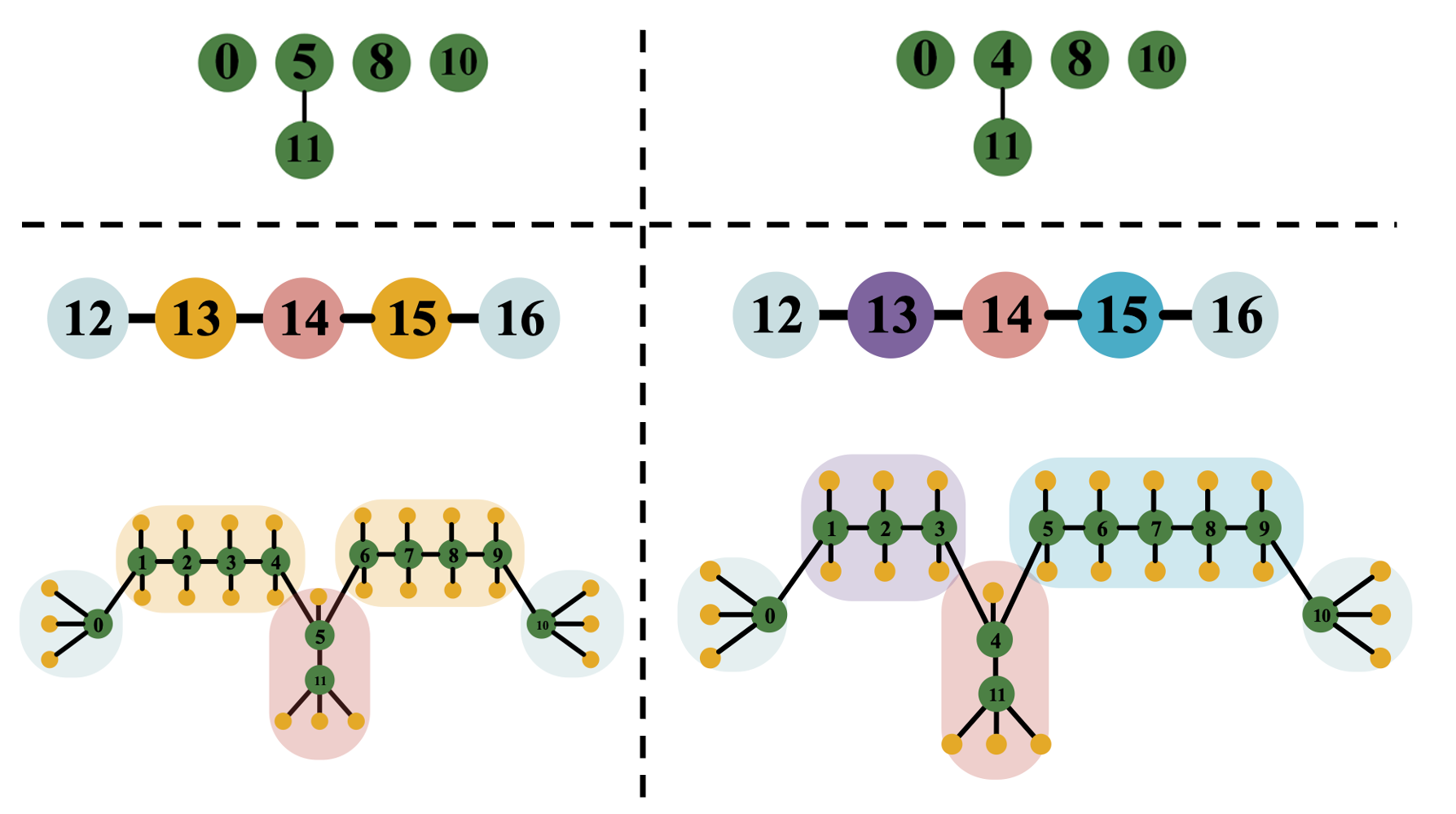
For the graph classification task, one GNN aims to learn one representation vector for each input graph to predict the graph label, and it is related to the interactions between long distance pairs (Jain et al., 2021), e.g., counting local substructures (Dwivedi et al., 2022). Therefore, how effectively embracing long-range dependencies is the key factor in designing neural networks. However, existing methods mentioned in Section 2.1.1 and 2.1.2 are deficient in capturing long-range dependencies. These methods update the graph structures either by generating the coarse graph or connecting to higher-order neighbors, which may result in insufficient discriminability, i.e., the discriminative graph structures may become indistinguishable anymore. For example, the pooling operations may generate the same coarse graph based on two distinguishable graphs, and the instances are provided in Appendix A.4.

Considering the deficiency of these methods, we turn to the stacking-based GNNs and search for better solutions to capture long-range dependencies. In general, scaling the model depth is the common way to improve the model performance in computation vision (Tan and Le, 2019; He et al., 2016), and deeper GNNs can enlarge the receptive field which enables the extraction of longer-range dependencies. Although, the over-smoothing problem is hard to evade in deep GNNs (Li et al., 2018; Xu et al., 2018), i.e., the connected nodes will have similar representations as the network becomes deeper, which will result in a performance drop on the node classification task. This problem hinders the development of deeper GNNs, and two- or three-layer shallow GNNs are widely used. However, as shown in proposition 1, we theoretically justify that the over-smoothing problem has smaller influence on the graph classification task compared with the node classification task. The proof is provided in Appendix A.1. Therefore, it is one potential solution to obtaining the long-range dependencies by stacking sufficient GNN layers. In this paper, we extract the long-range dependencies by stacking sufficient GNN layers as mentioned in Section 2.1.3. Compared with the aforementioned methods, it can preserve the graph structure information in the computational graph without modifying the graph structure.

Figure 1. (a): The illustrations of two molecule graphs ($C_{12}H_{26}$) where the green node is carbon and the orange node is hydrogen. (b): We visualize the computation graph used in the 2-layer GNNs for each node in the table. Two graphs have the same subtree distribution and lead to the same graph representation. (c): Especially, we visualize the computation graph for node 2 in $\mathcal{G}_{2}$ used in the 4-layer GNN. It contains $S1$ and $S3$ simultaneously, which is unique in $\mathcal{G}_{2}$.

Proposition 1.

Let $\mathcal{G}_{1}$ and $\mathcal{G}_{2}$ are two different graphs that satisfy: (a) have no bipartite components, and (b) at least one of the eigenvectors or eigenvalues are different. Then, for any learnable parameter W, $(I-L_{1}^{sym})^{\infty}\textbf{W}\neq(I-L_{2}^{sym})^{\infty}\textbf{W}$, where $L_{1}^{sym}$ and $L_{2}^{sym}$ are the symmetric Laplacian matrices of $\mathcal{G}_{1}$ and $\mathcal{G}_{2}$, respectively.

3.2. Design Needs for Stacking-based GNNs

When using the stacking-based GNNs to capture the long-range dependencies, two aspects affect the utilization of long-distant neighbors, i.e., the GNN depth and the skip-connection schemes. The former reflects the longest distance one node can access, and the latter is related to the information mixing from different ranges of neighbors. Therefore, to effectively capture the long-range dependencies, these two design needs should be considered when designing the stacking GNNs in this paper.

3.2.1. Depth needs to be sufficient.

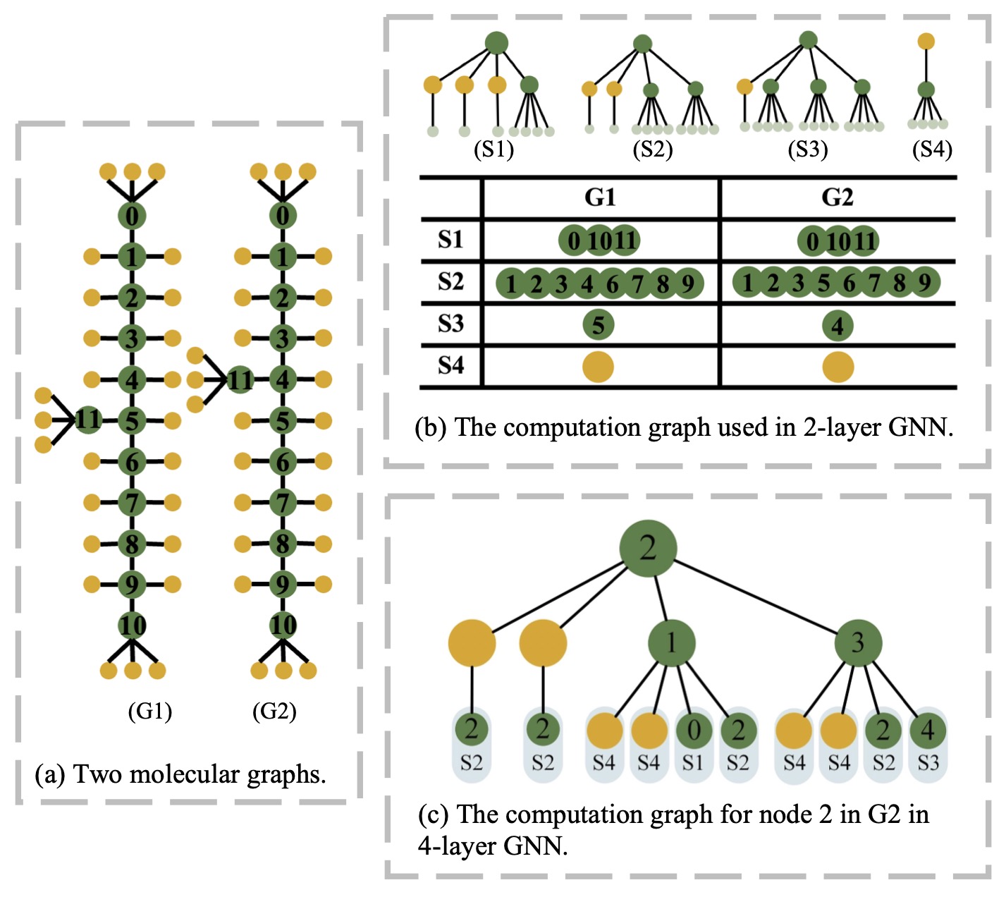
By stacking more aggregation operations, deeper GNNs can incorporate the interactions from more distant neighbors which affect the prediction results. We theoretically justify the discriminative power, i.e., how well GNNs with different depths can distinguish the non-isomorphic graphs, in Proposition 2. The proof is proved in Appendix A.2. Use the cases shown in Figure 1 (a) as an example, the key difference between these two graphs is the graph structures within nodes 0 and 11, and these two graphs can be distinguished by the 1-WL test in the $4$-th iteration. As shown in Figure 1 (b), two-layer GNN cannot distinguish two graphs since the same computation graphs are obtained in two molecular graphs, and the same graph representation vector will be obtained based on this. However, as shown in Figure 1 (c), the visualized computation graph of node $2$ in $\mathcal{G}_{2}$ contains $S1$ and $S3$ simultaneously, while it cannot be achieved in $\mathcal{G}_{1}$. On top of this, a four-layer GNN can distinguish these two graphs. Combined with the 1-WL test, deeper GNNs are more expressive than shallower ones, while two- or three-layer GNNs are widely used in the graph classification task. Therefore, it is necessary to enlarge the model depth when capturing the long-range dependencies in the graph classification.

Proposition 2.

For any two graphs $\mathcal{G}_{1}$ and $\mathcal{G}_{2}$ which are non-isomorphic and can be distinguished by the first-order Weisfeiler-Lehman test in $k$-th iteration, one aggregation-based $L$-layer GNN $\mathcal{A}_{L}:\mathcal{G}\rightarrow\mathbb{R}^{d}$ can come up the following conclusions:

$$\mathcal{A}_{L}(\mathcal{G}_{1})\neq\mathcal{A}_{L}(\mathcal{G}_{2}),L\geq k,$$

$$\mathcal{A}_{l}(\mathcal{G}_{1})=\mathcal{A}_{l}(\mathcal{G}_{2}),\forall\,0\leq l<k.$$

Figure 2. The performance comparisons with GNNs in different model depth and skip-connection schemes. Each dataset has a different number of graphs in diameter of $5$ and $14$. Graph label is determined by its diameter. The details are provided in Appendix A.3.

3.2.2. Skip-connection needs to be adaptive.

Based on proposition 2, different graph pairs may have different distinguishable iteration $k$ in the 1-WL test. Therefore, it is unreasonable to incorporate the distant neighbors with only one variety, i.e., only from the $k$-hop away, when facing those graphs in the datasets. In stacking-based GNNs, each node can increasingly expand the receptive field as the network goes deeper, and then designing the skip-connection schemes in GNN can make up for this deficiency since the information extracted from different ranges of neighbors can be mixed based on the skip-connections, on top of which the extracted information can be enriched.

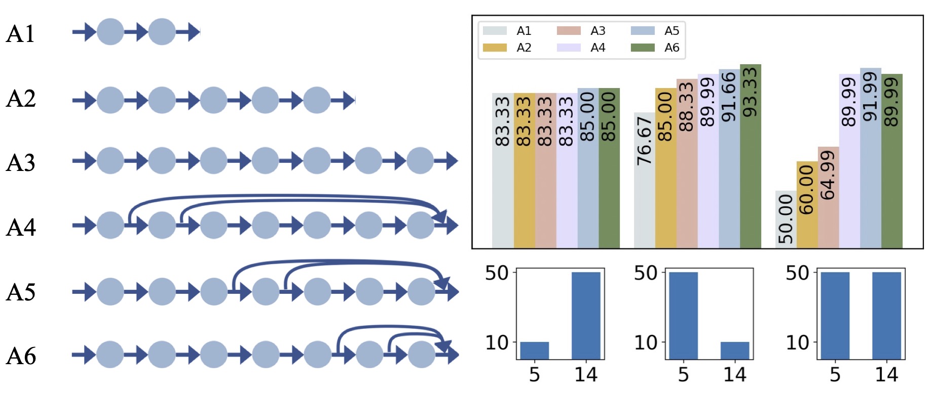
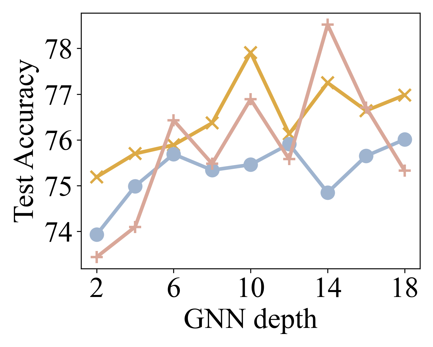
As shown in Figure 2, we design six GNNs with different model depths and skip-connection schemes, and then evaluate them on three datasets that have different graph diameter distributions. We observe that: (a) deeper GNNs achieve higher performance in general, which demonstrates the importance of sufficient large layer numbers in the graph classification task; (b) different skip-connection schemes result in diverse performances in each dataset, and they also have different ranks. Therefore, it is a necessity to design the skip-connections data-specifically (Zhao et al., 2020, 2021).

3.3. Designing Inter-layer Connections in Stacking-based GNNs

When using the stacking-based GNNs to extract the long-range dependencies, the model depth and the skip-connection schemes should be considered. These two designing needs can be unified by designing inter-layer connections, which correspond to the inter-layer connections between the consecutive and inconsecutive layers, respectively. To effectively extract the long-range dependencies, we adopt NAS to design the inter-layer connections in GNNs, on top of which the GNN depth and skip-connection schemes will be obtained adaptively.

Figure 3. (a) GNN framework used to design the inter-layer connections. (b) Cell-based GNN architecture. Each cell contains $B/C$ ($B=8$ and $C=2$ for example) aggregation operations and a post-processing operation. (c) One architecture design example. For aggregation operation 3, the connection from operation $0$ is unused, and two inputs from operation $1$ and $2$ are merged with operation SUM, on top of which the aggregation operation $3$ can be operated.

3.3.1. Architecture framework

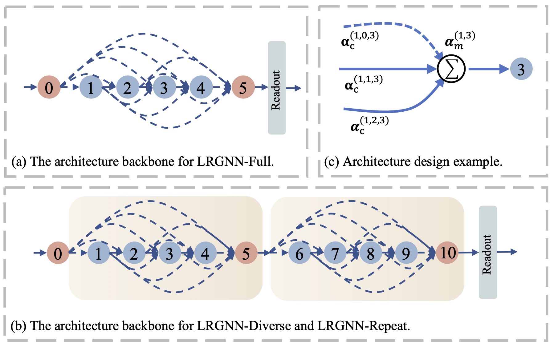
As shown in Figure 3 (a), we provide a unified framework to design the inter-layer connections in GNNs, which is constructed with an ordered sequence of $B$ aggregation operations ($B=4$ and GCN (Kipf and Welling, 2016) operation for example). Motivated by GraphGym (You et al., 2020), we provide one pre-processing operation $0$ and one post-processing operation $B+1$, each of which is one two-layer MLP (Multilayer Perceptron) to support the integration in the following procedures. At the end of this framework, one readout operation is provided to learn the graph representations. By deciding whether to use these inter-layer connections, i.e., the dashed lines shown in the framework, we can obtain GNNs with different depths and skip-connections to extract the long-range dependencies.

3.3.2. Designing search space based on the framework.

We provide a set of candidates to construct the search space. As shown in Figure 3 (a), the connections among different operations (with dashed lines) are learnable, and each of them is an “on-off switch” when utilizing features, i.e., only “used” and “unused” states existed. Therefore, we provide two candidate choices to represent these two states on each learnable connection in the framework, i.e., $\mathcal{O}_{c}=\{$ON, OFF$\}$. They can be represented as $o(\textbf{H})=\textbf{H}$ and $o(\textbf{H})=\textbf{0}$, respectively. For aggregation operations and the post-processing operation, more than one connection may be used. A straightforward manner is to add up these selected features. To further improve the model expressiveness, we provide one merge operation to incorporate these selected features. Based on the literature, we provide six candidates to merge them with the concatenation, LSTM cell, attention mechanism, summation, average and maximum. Then the merge operations are denoted as $\mathcal{O}_{m}=\{$CONCAT, LSTM, ATT, SUM, MEAN, MAX $\}$. For readout operation, we provide seven candidates to obtain the graph representation vector and it can be denoted as $\mathcal{O}_{r}=\{$GMEAN, GMAX, GSUM, GSORT, GATT, SET2SET , MEMA$\}$. These candidates represent: three simple global mean, max and sum functions; four readout operations derived from (Zhang et al., 2018), (Li et al., 2016), (Vinyals et al., 2016) and (Lee et al., 2019), respectively.

As shown in Figure 3 (a), the operations used in each learnable connection are designed independently, and then different depth and skip-connection schemes will be obtained in GNNs. Meanwhile, designing the merge and readout operations can further improve the expressiveness of GNNs  (Xu et al., 2019). This variant is denoted as LRGNN-Full in this paper.

As mentioned in Section 3.2.1, the GNN depth should be sufficiently large, which demonstrates the large number of aggregation operations in the framework. Then, the search space size is growing exponentially along with the increasing number of aggregation operations. Considering the search efficiency, we adopt the cells which are widely used in NAS (Liu et al., 2019; Pham et al., 2018) and provide one cell-based framework as shown in Figure 3 (b). Each cell can be treated as one basic unit to design the stacking-based GNNs. $C$ cells are provided and then these $B$ aggregation operations are assigned to the cells equally. The operations in each cell can be learned independently, and we will obtain different cells with diverse connection schemes and merge operations in the searched GNN, which is dubbed LRGNN-Diverse. On the contrary, we can share the operations among cells, on top of which the same cell is used in the searched GNN, which is dubbed LRGNN-Repeat in this paper.

3.3.3. Architecture search from the search space.

The architecture design can be formulated as the bi-level optimization problem as shown in the following:

$$\min\nolimits_{\bm{\alpha}\in\mathcal{A}} \;\mathcal{L}_{\text{val}}(\textbf{W}^{*}(\bm{\alpha}),\bm{\alpha}),$$

$$\ \text{\;s.t.\;}\textbf{W}^{*}(\bm{\alpha}) =\operatorname*{arg\,min}\nolimits_{\textbf{W}}\mathcal{L}_{\text{train}}(\textbf{W},\bm{\alpha}),$$

$\mathcal{A}$ represents the search space, and $\bm{\alpha}$ represents the neural architecture in $\mathcal{A}$. W represents the parameters of a model from the search space, and $\textbf{W}^{*}(\bm{\alpha})$ represents the corresponding operation parameter after training. $\mathcal{L}_{\text{train}}$ and $\mathcal{L}_{\text{val}}$ represent the training and validation loss, respectively. In this paper, $\bm{\alpha}=\{\bm{\alpha}_{c},\bm{\alpha}_{m},\bm{\alpha}_{r}\}$ has three components need to be designed. As shown in Figure 3 (c), $\bm{\alpha}^{(c,i,j)}_{c}\in\mathbb{R}^{|\mathcal{O}_{c}|}$ represent the learnable connections between the operation $i$ and $j$ in $c$-th cell. $\bm{\alpha}^{(c,i)}_{m}\in\mathbb{R}^{|\mathcal{O}_{m}|}$ represent the merge operation used in the aggregation operation $i$ in $c$-th cell. The LRGNN-Full variant adopts $c=1$ merely, while LRGNN-Repeat share the parameters $\bm{\alpha}^{(i,j)}_{c}$ and $\bm{\alpha}^{(i)}_{m}$ cross cells.

The differentiable method is employed in this paper which is widely used in the NAS methods (Liu et al., 2019; Xie et al., 2018). We adopted the Gumbel Softmax to relax the search space directly. As shown in the following:

(1) $$c_{k} =g(\mathcal{O},\bm{\alpha},k)=\frac{\exp((\log\bm{\alpha}_{k}+\textbf{G}_{k})/\lambda)}{\sum_{j=1}^{\left|\mathcal{O}\right|}\exp((\log\bm{\alpha}_{j}+\textbf{G}_{j})/\lambda)},$$

$\textbf{G}_{k}=-\log(-\log(\textbf{U}_{k}))$ is the Gumble random variable, and $\textbf{U}_{k}$ is a uniform random variable, $\lambda$ is the temperature of softmax. As shown in Figure 3 (c), we use the aggregation operation $3$ as an example, the output can be represented as

(2) $$\textbf{H}^{(i,3)} =\sum_{k=1}^{|\mathcal{O}_{c}|}c_{k}o_{k}(\textbf{H}^{i}),c_{k}=g(\mathcal{O}_{c},\bm{\alpha}^{(1,i,3)}_{c},k),$$

(3) $$\textbf{H}^{3}_{in} =\sum_{k=1}^{|\mathcal{O}_{m}|}c_{k}o_{k}(\{\textbf{H}^{(i,3)}|0\leq i\leq 2\}),c_{k}=g(\mathcal{O}_{m},\bm{\alpha}^{(1,3)}_{m},k),$$

(4) $$\textbf{H}^{3} =\text{AGG}(\textbf{A},\textbf{H}^{3}_{in}).$$

$\textbf{H}^{i}$ is the output feature matrix of operation $i$, and $\textbf{H}^{(i,3)}$ represent the results collected based on the connection from operation $i$ to operation $3$. Then, these selected features are merged and the results are denoted as $\textbf{H}^{3}_{in}$, on top of which one aggregation operation AGG can be applied and the output of operation $3$, i.e., $\textbf{H}^{3}$, will be generated. The graph representation can be generated as shown in the Alg. 1 in Appendix A.5. We optimize the parameters $\bm{\alpha}$ and W with the gradient descent, and the details are provided in Alg. 2 in Appendix A.5. After the training finished, we obtained the searched GNNs by preserving the operations with the largest weights.

In summary, LRGNN aims to design the inter-layer connections in deep stacking-based GNNs to capture the long-range dependencies in the graph classification task. Compared with existing methods which use shallow GNNs or only design deep GNNs in the node classification task, LRGNN evokes the importance of deep stacking-based GNNs in the graph classification task, and the rationality has been justified in Section 3.1. Besides, the methods which aim to design adaptive aggregation operations are orthogonal with LRGNN, and they can be incorporated into this paper directly. In the following, we empirically evaluate the rationality and effectiveness of LRGNN.

4. Experiments

We evaluate the proposed LRGNN against a number of SOTA methods and widely used GNNs, with the goal of answering the following research questions:

Q1: How does the over-smoothing problem and two design needs empirically affect the performance of stacking-based GNNs in the graph classification task? (Section 4.2)?

Q2: How does the proposed LRGNN compare to other methods when extracting the long-range dependencies (Section 4.3)?

Q3: How does each component affect the method performance, i.e., the merge and readout operations used in the search space, and the cell-based search space designed considering the search efficiency (Section 4.4).

4.1. Experimental Settings

4.1.1. Datasets

As shown in Tab. 1, we use five datasets with different graph diameters from different domains. NCI1 and NCI109 are datasets of chemical compounds (Wale and Karypis, 2006). DD and PROTEINS datasets are both protein graphs (Dobson and Doig, 2003). IMDB-BINARY dataset is movie-collaboration datasets (Yanardag and Vishwanathan, 2015).

Table 1. Statistics of the datasets from three domains.

Dataset	# of Graphs	# of Feature	# of Classes	Avg.# of Nodes	Avg.# of Edges	Domain
NCI1	4,110	89	2	29.87	32.3	Chemistry
NCI109	4,127	38	2	29.69	32.13	Chemistry
DD	1,178	89	2	384.3	715.7	Bioinfo
PROTEINS	1,113	3	2	39.1	72.8	Bioinfo
IMDB-BINARY	1,000	0	2	19.8	96.5	Social

4.1.2. Baselines

We provide three kinds of baselines in this paper:

$\bullet$ For stacking-based GNNs, we adopt three baselines in this paper which use different skip-connection schemes: GCN (Kipf and Welling, 2016), ResGCN (Li et al., 2019) and GCNJK (Xu et al., 2018). We vary the GNN layers in $\{4,8,12,16\}$, and then report the best methods in Tab. 2 (More results can be found in Appendix B.1).

$\bullet$ We provide three pooling methods used in this task: DGCNN (Zhang et al., 2018) baseline with $8$-layer stacked GCN operations and the designed readout function; $2$-layer SAGPool (Lee et al., 2019) and DiffPool (Ying et al., 2018) baselines in which each layer has one GCN operation and one pooling operation.

$\bullet$ Considering the methods which incorporate the higher-order neighbors, we provide four baselines. Firstly, we use the 4-layer stacked GCN, and in each layer nodes aggregate messages from the neighbors exactly one and two hops away. This baseline is denoted as TwoHop(L4) in this paper (Abu-El-Haija et al., 2019). For GCNFA(L8) (Alon and Yahav, 2021) baseline, we use the 8-layer stacked GCN in which the $8$-th layer uses the fully-adjacency matrix instead. For GCNVIR(L8) (Pham et al., 2017), we use the $8$-layer stacked GNN, and in each layer, we add one virtual node. For GraphTrans (Jain et al., 2021), we adopt the small variant in this paper which use three GCN layers and four transformer layers.

Compared with these baselines, we provide four LRGNN variants: LRGNN-Full with 8 and 12 aggregation operations, which denoted as B8C1 and B12C1, respectively; LRGNN-Repeat and LRGNN-Diverse with 12 aggregation operations and 3 cells, which denoted as Repeat B12C3 and Diverse B12C3, respectively.

4.1.3. Implementation details

For all datasets, we perform 10-fold cross-validation to evaluate the model performance and an inner holdout technique with a 80%/10%/10% training/validation/test for model training and selection. In this paper, we set the training and finetuning stages to get the performance for the proposed LRGNN. In the training stage, we derived the candidate GNNs from the corresponding search space. For the searched GNNs and the baselines, we fine-tune the hyper-parameters of these methods in the finetuning stage. The details are provided in Appendix B.1.

4.2. The Rationality of LRGNN

Table 2. Performance comparisons. We first show the average diameters of the datasets. Then, we report the mean test accuracy and the standard deviations based on the 10-fold cross-validation data. For the proposed method, BICJ represent these architectures contains $i$ aggregation operations and $j$ cells. $[Li]$ represents the model depth is $i$. “OOM” means out of memory. The best result in each group is underlined, and the best result in this dataset is highlighted in gray. The average rank on all datasets is provided and the Top-3 methods are highlighted. For GCNFA and GraphTrans, the averaged rank is calculated based the other four datasets.

	Method	NCI1	NCI109	DD	PROTEINS	IMDB-BINARY	Avg. rank
	Diameter	13.33	13.13	19.90	11.57	1.86
	GCN	78.98(3.24) [L16]	76.64(1.04) [L16]	75.63(2.95) [L16]	75.11(4.51) [L8]	73.80(5.13) [L4]	7.4
	ResGCN	77.88(2.24) [L12]	76.71(1.83) [L16]	76.65(2.73) [L8]	75.11(3.22) [L8]	73.70(5.70) [L12]	7.2
Stacking	GCNJK	79.24(2.11) [L12]	75.91(3.61) [L12]	73.16(5.12) [L8]	75.24(4.15) [L8]	74.20(3.76) [L16]	6.6
	DGCNN(L8)	76.08(1.03)	74.58(3.99)	61.63(5.33)	73.95(3.04)	71.70(3.65)	11.6
	SAGPool	72.23(3.68)	69.78(2.26)	70.52(5.48)	71.89(4.03)	73.40(3.02)	12
Pooling	DiffPool	75.04(1.98)	71.48(2.46)	77.85(3.53)	75.11(2.14)	72.27(4.47)	9.2
	TwoHop(L4)	76.42(3.83)	75.33(2.15)	74.53(5.24)	75.30(4.27)	72.40(5.61)	8
	GCNVIR(L8)	70.32(4.32)	67.99(2.97)	71.98(4.34)	71.08(3.14)	71.50(4.90)	13.2
	GCNFA(L8)	76.39(3.72)	73.93(2.87)	OOM	74.31(4.16)	73.60(5.62)	10.25
	GraphTrans	82.04(1.43)	80.18(1.97)	OOM	75.12(4.89)	74.00(5.74)	4.75
Higher- order	Full B8C1	81.82(1.74) [L4]	81.39(1.92) [L6]	78.01(3.69) [L6]	75.39(4.40) [L6]	76.20(5.18) [L4]	1.6
	Full B12C1	82.51(1.37) [L7]	80.64(2.46) [L7]	78.18(2.02) [L9]	75.29(4.51) [L3]	74.50(3.31) [L5]	2.4
	Repeat B12C3	81.31(1.68) [L6]	80.79(1.24) [L6]	77.25(2.90) [L6]	75.30(4.77) [L3]	74.20(5.41) [L6]	3.6
LRGNN	Diverse B12C3	80.97(2.73) [L6]	80.98(1.96) [L9]	77.67(3.35) [L5]	74.93(5.15) [L7]	74.20(3.35) [L5]	4.8

4.2.1. The importance of sufficient model depth

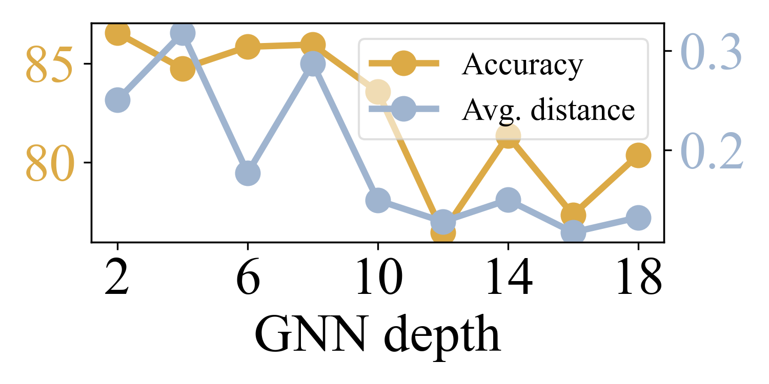
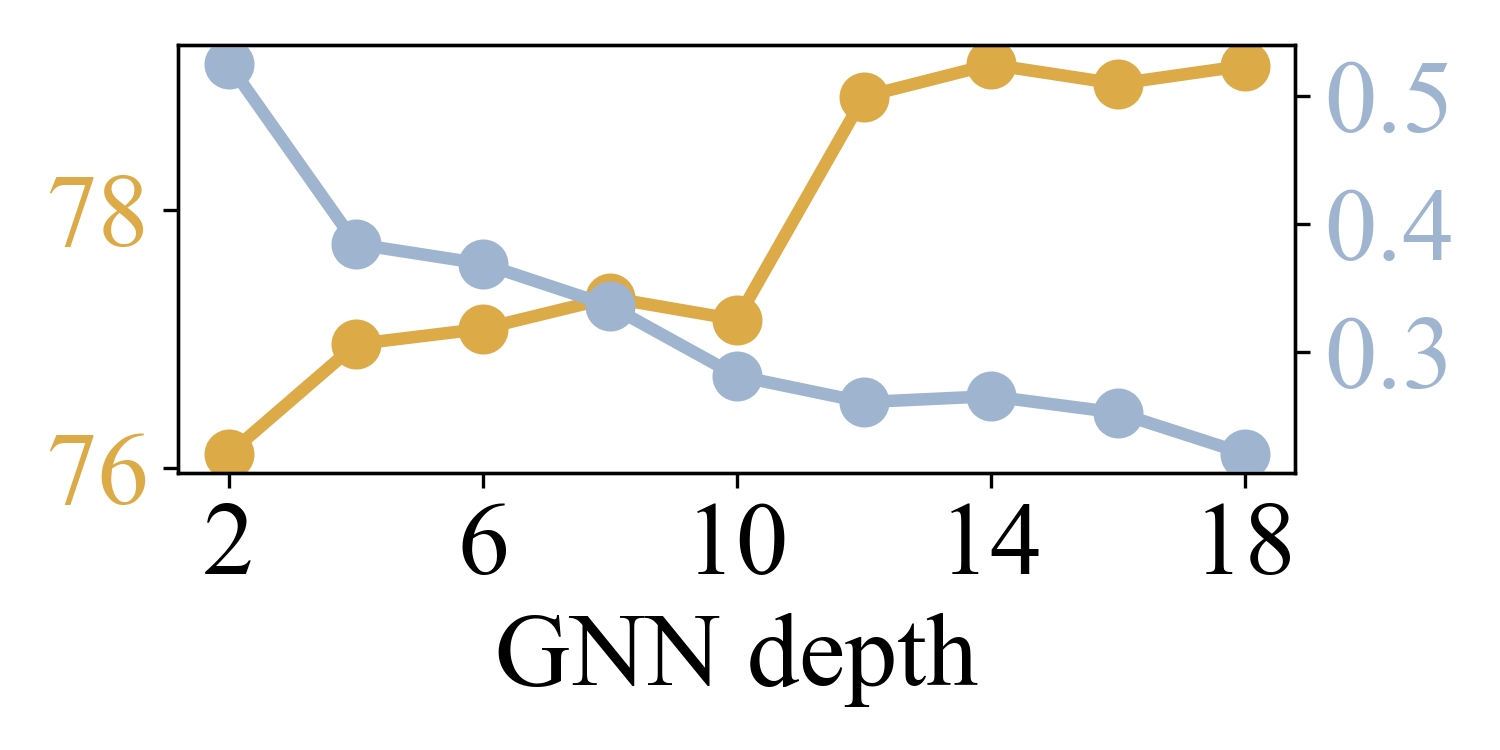
In this paper, we use the averaged node pair distance, which is calculated based on $D(h_{i},h_{j})=\|\frac{h_{i}}{\|h_{i}\|_{1}}-\frac{h_{j}}{\|h_{j}\|_{1}}\|_{1}$, to evaluate the over-smoothing problem. As shown in Figure 4, the lower distance values are observed on two datasets as the network goes deeper, which demonstrates the smoother features between node pairs are observed and the over-smoothing problem appeared in both the node classification and graph classification tasks. However, the upward trend of model performance is apparent in the NCI1 dataset, while the opposite trend is observed in the Cora dataset. It indicates the smaller influence of the over-smoothing problem on the graph classification task compared with the node classification task. Therefore, stacking sufficient layers to obtain the long-range dependencies is a feasible way.

Figure 4. The test accuracy and the averaged distance comparisons on the node classification dataset Cora (Left) and graph classification dataset NCI1 (Right).

4.2.2. The necessity of adaptive skip-connections

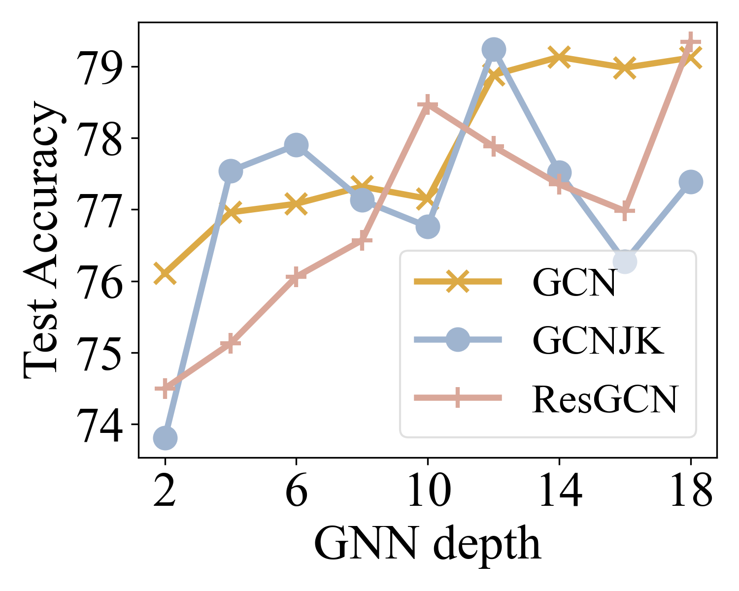
As mentioned in Section 3.2.2, designing adaptive skip-connections can enhance the information utilization from different ranges of neighbors. In this part, we empirically evaluate the skip-connection schemes on two real-world datasets. As shown in Figure 5, GNNs with different skip-connection schemes have diverse performances in each dataset. Besides, the SOTA performance is achieved by designing the skip-connections, i.e., ResGCN achieves the SOTA performance on the NCI109 dataset and GCNJK ranks first on the NCI1 dataset. Given the fixed GNN depth, these three baselines have different ranks on two datasets. All these results demonstrate the necessity of data-specific skip-connection schemes.

Figure 5. The influence of different skip-connection schemes on NCI1 (Left) and NCI109 (Right) datasets.

In summary, sufficient GNN depth and adaptive skip-connection schemes are empirically important for stacking-based GNNs in extracting the long-range dependencies. In the following, we compare the proposed LRGNN with the SOTA methods to show its effectiveness.

4.3. The Effectiveness of LRGNN

As shown in Table 2, the variants B8C1, B12C1 and LRGNN-Repeat B12C3 can outperform all baselines, which demonstrates the effectiveness of the LRGNN method by designing the inter-layer connections in GNNs to utilize the long-range dependencies adaptively. Besides, for these methods which achieve the best results on these datasets (the results highlighted in gray in Tab. 2), we observe that the model depth in these methods are very close to the graph radius (diameter/$2$). This observation highlights the significance of sufficient model depth in GNNs. LRGNN-Repeat and LRGNN-Diverse variants constrain the search space and group the aggregation operations into different cells. Compared with LRGNN-Full, these two variants have fewer parameters based on the same aggregation operations (see Tab. 3), which enables the explorations on much deeper GNNs. However, they have limited search space, which may filter out the expressive architectures and lead to a performance decrease as shown in Tab. 2.

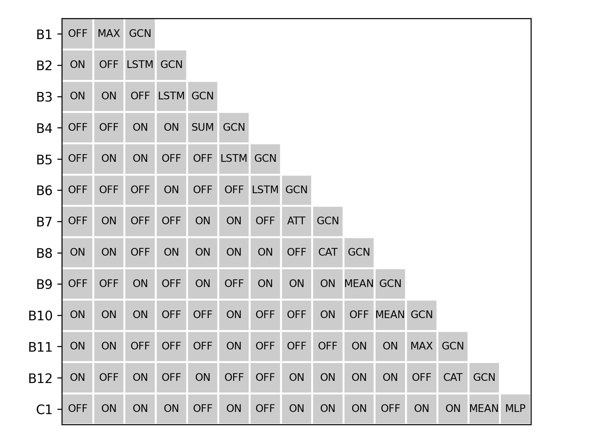
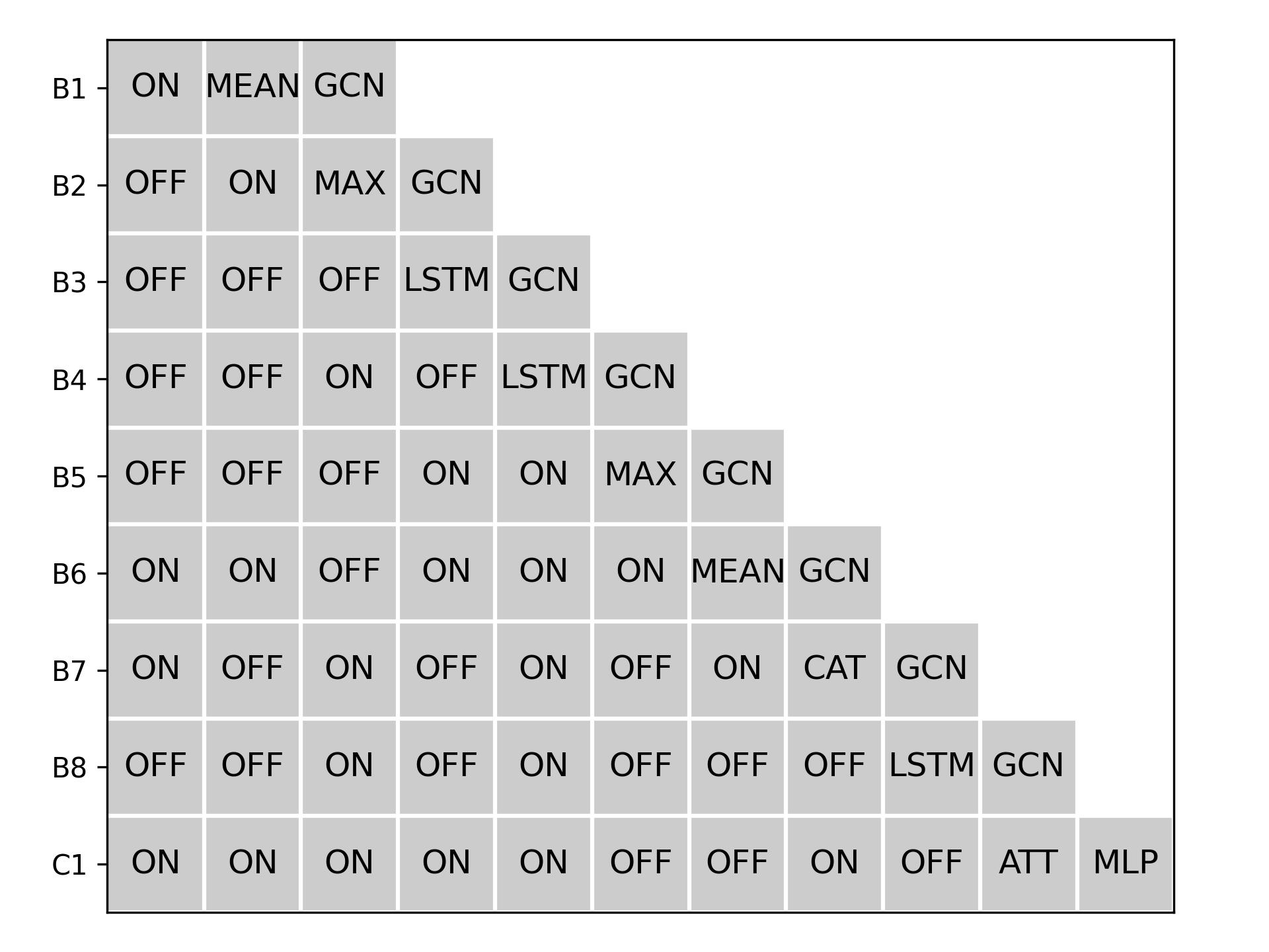
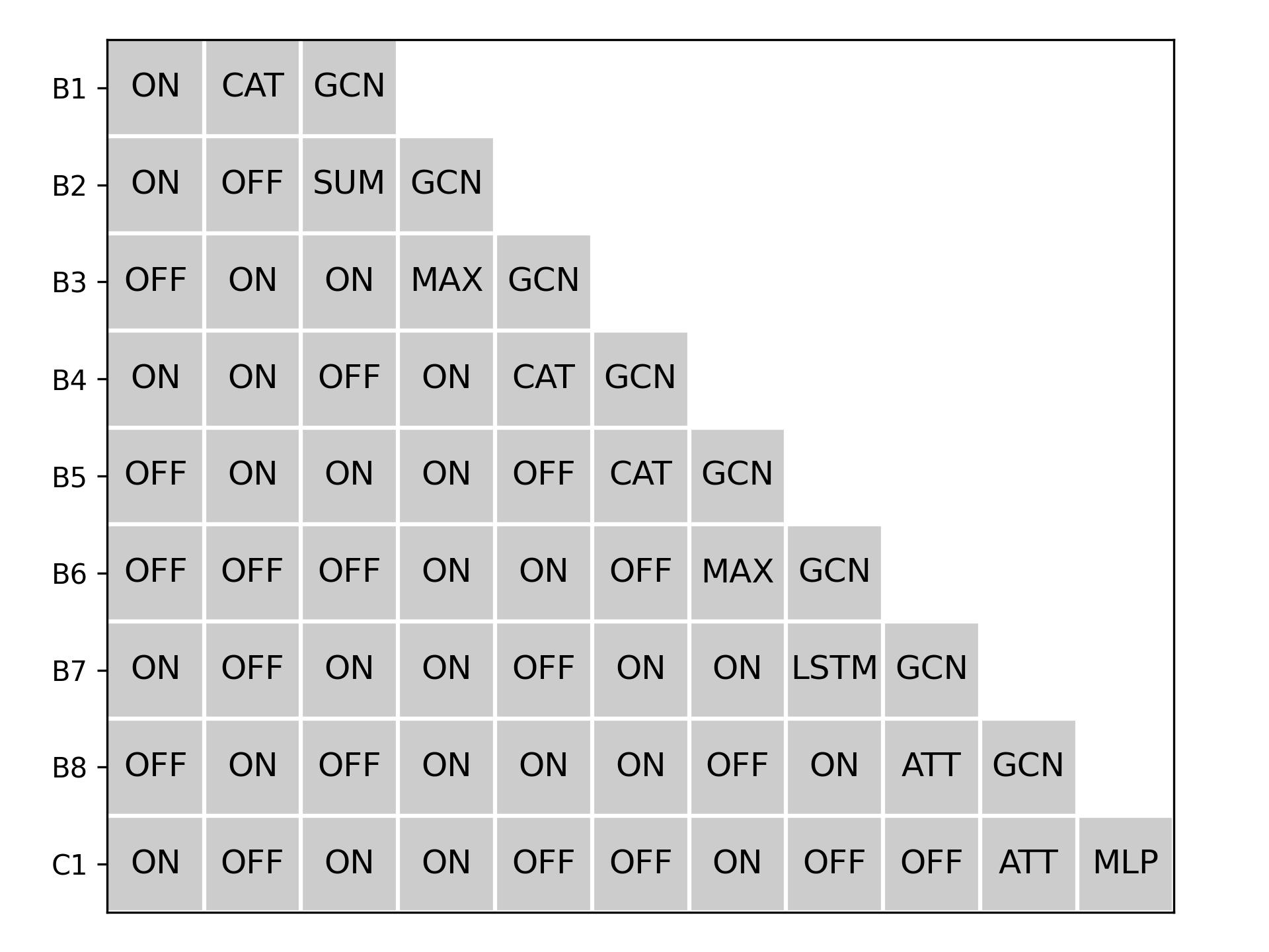
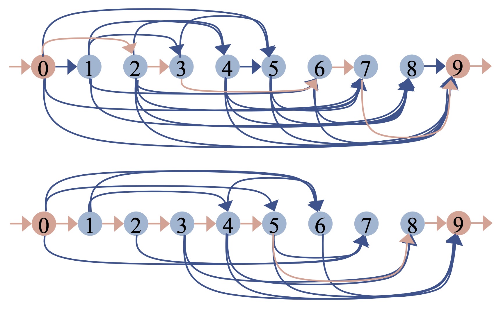
We visualize the searched inter-layer connections of LRGNN-Full B8C1 in Figure 6, and more results can be found in Appendix B.2. It is obvious that different inter-layer connection schemes are obtained on different datasets, and each operation has its own preference for turning on the connections from previous operations. The connections between the consecutive layers are emphasized in the NCI109 dataset, while the connections between the inconsecutive layers are widely used in the NCI1 dataset. We highlight one of the longest paths in the searched GNNs, and the searched architecture on the NCI109 datasets is deeper than that on the NCI1 dataset. Combine with the SOTA performance in Tab. 2, the effectiveness of designing inter-layer connections is obvious.

Figure 6. The searched inter-layer connections of LRGNN-Full B8C1 on NCI1 (Top) and NCI109 (Bottom) datasets. We highlight one of the longest path in the GNNs, on top of which the model depth can be obtained.

Compared with the stacking-based methods, we observe that three baselines could achieve higher performance with more GNN layers. Besides, by utilizing different skip-connection schemes, ResGCN and GCNJK achieve higher performance than GCN baseline which has no skip-connections. The performance benefits a lot from the inter-layer connections, and the proposed LRGNN achieves better performance by designing the inter-layer connections adaptively. As to the other two kinds of baselines, GraphTrans has the strongest ability in modeling the long-range information with the help of the Transformer module, which has been proved in the related methods (Jain et al., 2021; Ying et al., 2021). Besides, the global pooling method DGCNN and two hierarchical pooling methods, i.e., SAGPool and DiffPool, have different performances on these datasets, and no absolute winner from these two kinds of pooling methods on all datasets, which is consistent with existing methods (Mesquita et al., 2020; Errica et al., 2020; Wei et al., 2021). The grouping-based methods, e.g., DiffPool, achieves higher ranks than the selection-based method SAGPool in general. Compared with these methods, LRGNN has better performance due to the strong ability of the stacking-based GNNs in preserving the graph structures.

4.4. Ablation Study

To evaluate the contributions of different components, in this section, we conduct ablation studies on the cell-based search space, and two operations added to improve the model expressiveness. Considering the limited space, we show the ablation study experiments on aggregation operation and the search algorithm in Appendix B.3.

Table 3. Evaluations on the cell-based architecture. We show the comparisons of the performance, the parameter numbers(M) in the supernet and the search cost (GPU second) in the training stage.

	DD	PROTEINS
Full B4C1	77.16(2.98) / 0.23M / 469s	75.30(4.67) / 1.01M / 247s
Full B8C1	78.01(3.69) / 0.92M / 1306s	75.39(4.40) / 3.62M / 394s
Full B12C1	78.18(2.02) / 2.28M / 1458s	75.29(4.51) / 9.06M / 573s
Repeat B12C3	77.25(2.90) / 0.24M / 1226s	75.30(4.77) / 1.05M / 500s
Diverse B12C3	77.67(3.35) / 0.68M / 1286s	74.93(5.15) / 2.79M / 545s
Full B16C1	OOM	74.48(3.89) / 18.39M / 879s
Repeat B16C4	77.24(3.59) / 0.25M / 1697s	74.48(4.75) / 1.07M / 622s
Diverse B16C4	77.59(3.24) / 0.94M /1404s	75.56(4.12) / 3.68M / 665s

4.4.1. The evaluation on cell-based search space

Considering the search efficiency, we provide one cell-based framework which can constrain the search space by designing the connections in cells. To evaluate the efficiency and effectiveness of the cell-based architectures, we varify the cell numbers and the results are shown in Tab. 3 It is obvious that LRGNN-Full cannot work on DD dataset given $16$ aggregation operations in one cell, while it can work when we assign these 16 aggregation operations into $4$ cells. With the same GPU, the cell-based LRGNN-Repeat and LRGNN-Diverse raise the ceiling of the GNN depth compared with the LRGNN-Full. Besides, the Repeat and Diverse variants have fewer parameters and search costs, which demonstrates the search efficiency when using cells. As to the performance, these variants have a smaller search space, and they may filter out the expressive architectures. Therefore, they may be outperformed by LRGNN-Full in some cases. As a conclusion, LRGNN-Full can achieve higher-performance while the other two variants have advantages in the training efficiency.

4.4.2. The evaluation of the merge and readout operations.

In the search space, we provide the merge operation and readout operation to improve the model expressiveness as mentioned in Section 3.3. Then, we conduct ablation studies on these two operations to show their effectiveness in improving the model performance.

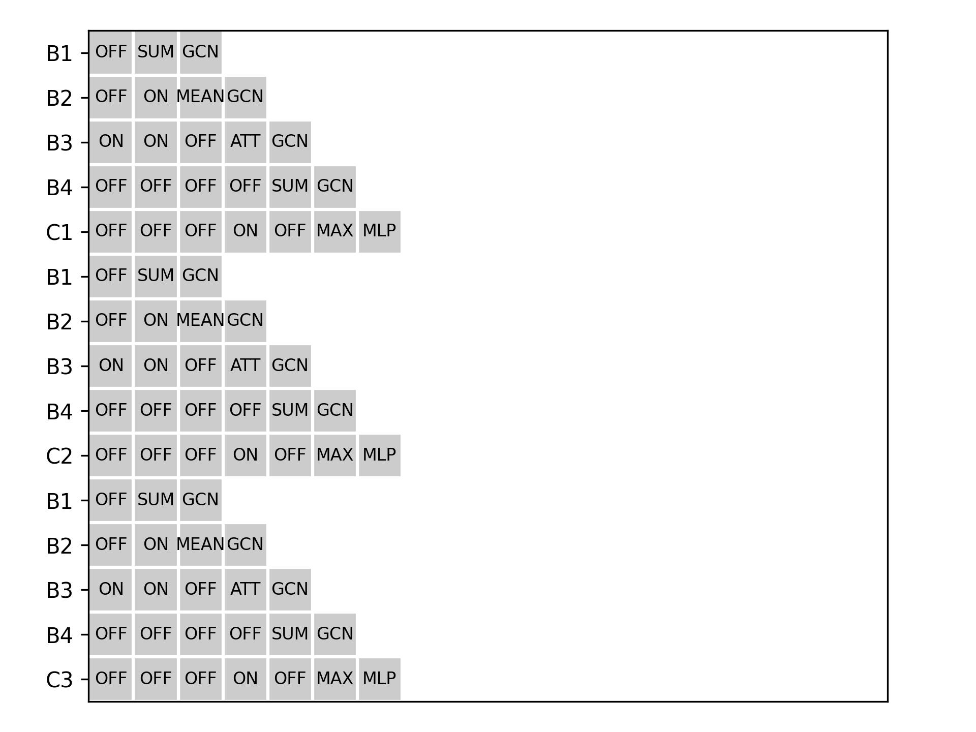
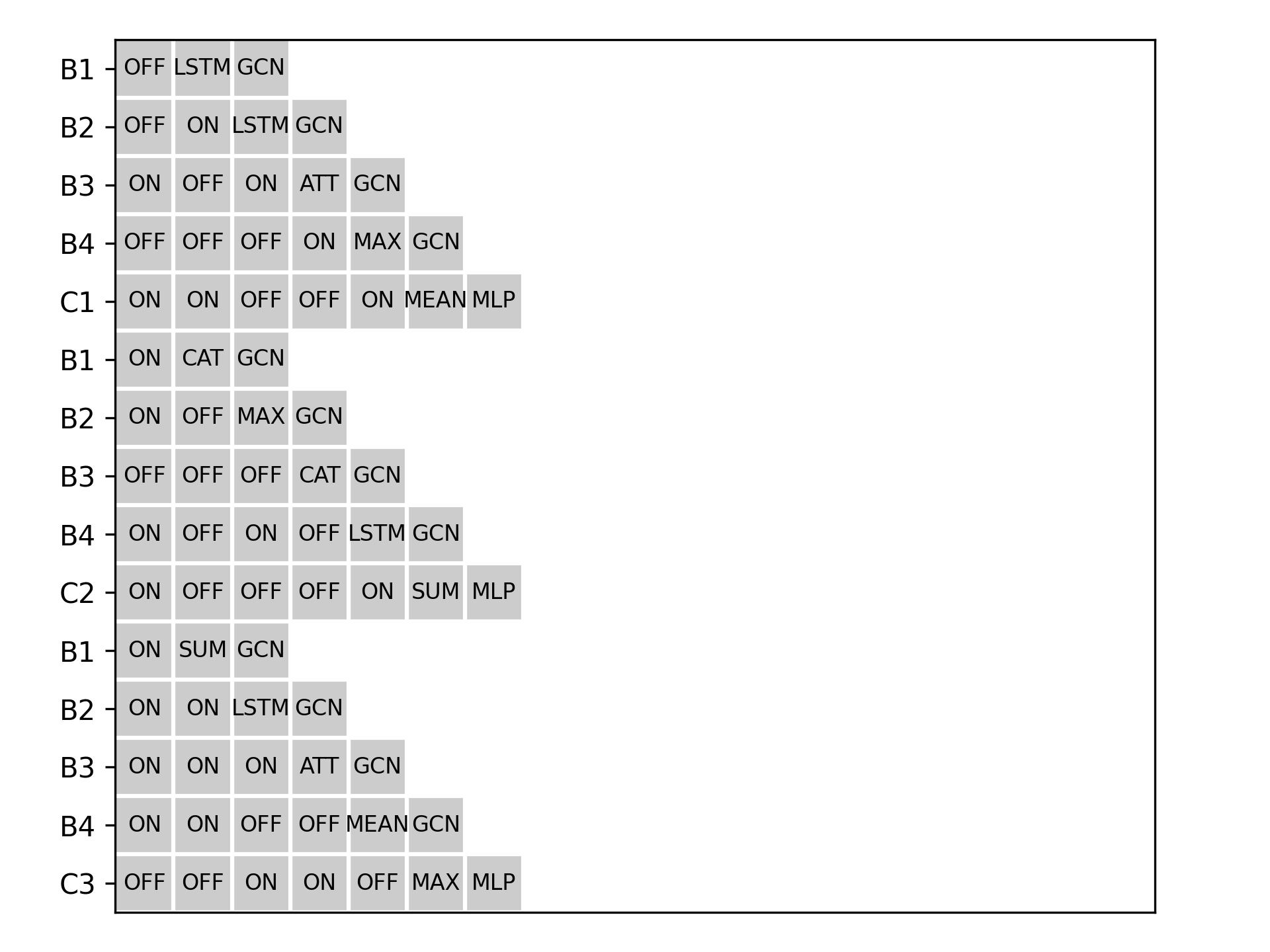
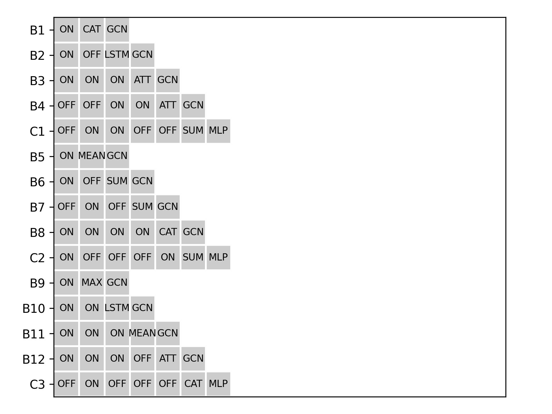
In this paper, we provide a set of merge operations that are expected to improve the model expressiveness. As shown in Figure 7 (a), compared with LRGNN which designs the merge operations adaptively, using the pre-defined merge operations may not achieve higher performance in general. The searched results are visualized in Appendix B.2, from which we can observe the different merge operations are utilized. Combine with better performance, the effectiveness to design the merge operations adaptively is obvious.

Figure 7. Evaluations on the merge and readout operation. These methods are constructed based on LRGNN-Full B12C1 variant and different merge or readout operations.

The readout operation is responsible for generating the graph representation vector for the given graph. In this paper, we provide seven candidates and learn to design this operation adaptively. As shown in Figure 7 (b), LRGNN achieves the SOTA performance in three datasets, and all of them utilize the GSUM readout operation in the searched architectures. Besides, the baseline which uses the predefined readout operation GSUM achieves comparable performance as well. Nevertheless, using the other two readout operations lead to a performance drop, and then it is important to design the readout operation adaptively.

5. Conclusion

In this paper, we provide a novel method LRGNN to capture the long-range dependencies with stacking GNNs in the graph classification task. We justify that the over-smoothing problem has smaller influence on the graph classification task, and then employ the stacking-based GNNs to extract the long-range dependencies. Two design needs, i.e., sufficient model depth and adaptive skip-connections, are provided when designing the stacking-based GNNs. To meet these two design needs, we unify them into inter-layer connections, and then design these connections with the help of NAS. Extensive experiments demonstrate the rationality and effectiveness of the proposed LRGNN. For future work, we will evaluate the importance of different hops’ neighbors in different graph pairs, and then extract this information for each graph independently.

Appendix A Method

A.1. The Proof of Proposition 1

Proof.

It has been proved in Theorem 1 (Li et al., 2018) that $(I-L^{sym})^{\infty}\textbf{W}$ will converge to the linear combination of eigenvectors of eigenvalue 1. The satisfied graphs will converged to different points, which leads to differnt node features in these two graphs. Then, based on the Lemma 5 in (Xu et al., 2019), unique graph representation vector will be generated for each graph, and then two graphs be distinguished. ∎

A.2. The Proof of Proposition 2

Proof.

It has been proved in Theorem 3 (Xu et al., 2019) that GIN is as powerful as the 1-WL test. For two graphs which can be distinguished by 1-WL test at 4-th iteration, we can obtain that $\mathcal{A}_{k}^{GIN}(\mathcal{G}_{1})\neq\mathcal{A}_{k}^{GIN}(\mathcal{G}_{2})$ and $\mathcal{A}_{l}^{GIN}(\mathcal{G}_{1})=\mathcal{A}_{l}^{GIN}(\mathcal{G}_{2}),l\leq k$. Furthermore, the 1-WL test can distinguish two graphs after $k$-th iterations, and then $\mathcal{A}_{l}^{GIN}(\mathcal{G}_{1})\neq\mathcal{A}_{l}^{GIN}(\mathcal{G}_{2})$ also holds when $l>k$. ∎

We use the graphs in Figure 1(a) as an example. Two graphs have the same number of nodes, and all nodes have the same feature, e.g., all-one vector.

$\bullet$ $0$-layer GNN, which is constructed by MLP and a readout operation, cannot distinguish these two graphs. These two graphs have the same feature set, and MLPs with any layers will generate the same feature set for them as well. Based on these two graphs, any simple readout function designed on the node features will generate the same graph representation vectors. For example, take the mean or summation of all node embeddings as the graph-level representation vector. Set2Set operation (Vinyals et al., 2016) and SortPool (Zhang et al., 2018) have the same results. Therefore, the $0$-layer GNN cannot distinguish these two graphs.

$\bullet$ Shallow GNN cannot distinguish these two graphs. As shown in Figure 1 (b), we visualize the computation graph, which is denoted as $S1$-$S4$ in the figure, and nodes in each row use the same computation graph. In $2$-th iteration, 1-WL test will generate the same feature for the nodes in the same row. Therefore, 2-layer GIN, which is constructed by stacking two GIN aggregation operations and one readout function mentioned before, cannot distinguish two graphs as well. The $3$-layer GNN has the same situation.

$\bullet$ $4$-layer GNN can distinguish these two graphs. As shown in Figure 1 (c), we visualize the computation graph for node $2$ in $\mathcal{G}_{2}$. It contains the $S1$ and $S3$ graphs, while the nodes in $\mathcal{G}_{1}$ cannot achieve this. Therefore, two graphs have different feature sets in $4$-iteration in the 1-WL test. Therefore, $4$-layer GIN can distinguish two graphs.

In summary, capturing long-range dependencies is useful for the graph classification task, which is correlated with the 1-WL test.

A.3. Experimental Details for Figure 2

Datasets. Three datasets are constructed based on the NCI1 dataset which will be introduced in the following. For the first dataset, we sample 10 graphs with diameter $5$ and 50 graphs with diameter $14$. The other two datasets are constructed in the same way. The graph label is determined by the graph diameter. Therefore, these three datasets only have two labels. The diameter distribution for these datasets is provided in Figure 2.

Baselines. We provide six GNNs with different inter-layer connections as shown in Figure 2. Based on GCN aggregation operation, $A1$-$A3$ have different connection schemes between the consecutive layers and lead to different layer numbers, i.e., 2, 5, and 7, respectively. GNN $A4$-$A6$ use the different connections among inconsecutive layers.

Implementation details. We evaluate each GNN on three datasets. We fix the hidden dimension to 128, and use a batch size of 64, a fixed learning rate 0.01, and Adam optimizer. We visualize the averaged test accuracy in Figure 2 based on 10-fold cross-validation.

A.4. Limitations of Existing Methods

Using the graph pairs shown in Figure 1 as an example, we visualize the pooling results in Figure 8, in which two different graphs generate the same coarse graph after pooling operations. The selection-based pooling operations preserve the same node sets in two graphs, and the formulated coarse graphs are the same as the other. As to the grouping-based operations, the subgraphs in each colored block have similar features and are densely connected, and they are grouped into the corresponding new nodes in the coarse graph. The same coarse graphs are obtained as well.

Figure 8. The pooling results of $\mathcal{G}1$ (left) and $\mathcal{G}2$ (right). The coarse graphs in the top row is the results of the selection-based operations, and the bottom row is the results of grouping-based operations.

A.5. The details of the method

Using the LRGNN-Full as an example, we show the calculation of graph representations in Alg. 1, and show the optimization details in Alg. 2.

Algorithm 1 Generating the graph representations in LRGNN-Full

1:Input graph $\mathcal{G}=(\textbf{A},\textbf{H}^{input})$, the aggregation number $B$, aggregation operation AGG.

2:The graph representation $h_{\mathcal{G}}$.

3:Update the node feature in the pre-processing stage $\textbf{H}^{0}=f_{pre}(\textbf{H}^{input})$.

4:for $j=1,\ldots,B$ do

5:    Calculate the aggregation results $\textbf{H}^{j}$ based on Eq. (2),(3) and (4).

6:end for

7:Update the node feature in the post-processing stage $\textbf{H}^{F}=f_{post}(\textbf{H}^{B})$.

8:$h_{\mathcal{G}}=\sum_{i=1}^{|O_{r}|}c_{i}o_{i}(\textbf{A},\textbf{H}^{F})$ where $c_{k}=g(\mathcal{O}_{r},\bm{\alpha}_{r},k)$ . $//$ Readout

9:return $h_{\mathcal{G}}$

Algorithm 2 Designing the inter-layer connections for the stacking-based GNNs.

Training dataset $\mathcal{D}_{train}$, validation dataset $\mathcal{D}_{val}$, the search epoch $T$.

2:The searched GNN.

Random initialize the architecture parameters $\bm{\alpha}$ and operation parameter W.

4:while $t=1,\ldots,T$ do

    for each minibatch $\mathcal{G}_{b}\in\mathcal{D}_{train}$ do

6:       Calculate the graph representations $h_{\mathcal{G}_{b}}$ as shown in Alg. 1.

       Update W

8:    end for

    for each minibatch $\mathcal{G}_{b}\in\mathcal{D}_{val}$ do

10:       Calculate the graph representations $h_{\mathcal{G}_{b}}$ as shown in Alg. 1.

       Update $\bm{\alpha}$.

12:    end for

end while

14:Preserve the candidates with the largest weight in each learnable connection, merge and readout operations.

return The searched GNN.

Appendix B Experiments

B.1. Implementation Details

All models are implemented with Pytorch (Paszke et al., 2019) on a GPU RTX 3090 (Memory: 24GB, Cuda version: 11.2). We adopt the same data preprocessing manner provided by PyG and split data by means of a stratification technique with the same seed. We finetune the human-designed architectures and the searched architectures with the help of Hyperopt . In the finetuning stage, each GNN has 20 hyper steps. For LRGNN, a set of hyperparameters will be sampled from Tab. 4 in each step, and the baselines will be sampled from Tab. 5. Then we select the final hyper-parameters on the validation set, from which we can obtain the final performance of this GNN. For stacking-based baselines GCN and ResGCN, we vary the GNN layers in $\{4,8,12,16\}$, and then report the best methods in Tab. 2. The detailed results are shown in Tab. 6. Especially, for the GraphTrans baseline, we adopt the provided code  and split the data as mentioned before.

Table 4. Hyperparameter space in the finetuning stage for the proposed method.

Dimension	Operation
Embedding size	8, 16, 32, 64, 128, 256
Dropout rate	0, 0.1, 0.2, $\cdots$, 0.9
Learning rate	$[0.001,0.025]$
Optimizer	Adam, AdaGrad

Table 5. Hyperparameter space for human-designed baselines.

Dimension	Operation
Global pooling function	GMEAN, GSUM
Embedding size	8, 16, 32, 64, 128, 256, 512
Dropout rate	0, 0.1, 0.2,…,0.9
Learning rate	$[0.001,0.025]$

Table 6. Performance comparisons on the stacking-based baselines GCN, ResGCN and GCNJK with different layers.

Method	NCI1	NCI109	DD	PROTEINS	IMDBB
GCN(L4)	76.96(3.69)	75.70(4.03)	73.59(4.17)	74.84(3.07)	73.80(5.13)
GCN(L8)	77.32(3.17)	76.37(2.62)	74.01(2.85)	75.11(4.51)	71.60(4.30)
GCN(L12)	78.88(2.76)	76.13(2.15)	74.53(4.49)	74.30(3.79)	73.50(3.17)
GCN(L16)	78.98(3.24)	76.64(1.04)	75.63(2.95)	72.42(4.83)	71.50(4.94)
ResGCN(L4)	75.13(2.87)	74.10(5.183)	73.85(3.70)	74.40(5.22)	73.50(4.83)
ResGCN(L8)	76.57(2.306)	75.48(3.533)	76.65(2.73)	75.11(3.22)	73.20(6.36)
ResGCN(L12)	77.88(2.214)	75.58(2.027)	75.38(3.03)	73.40(5.62)	73.70(5.70)
ResGCN(L16)	76.98(2.907)	76.71(1.836)	75.46(3.29)	73.23(3.89)	73.19(3.61)
GCNJK(L4)	77.54(3.47)	74.99(3.54)	72.40(4.51)	73.21(2.71)	73.20(6.14)
GCNJK(L8)	77.13(3.29)	75.34(3.14)	73.16(5.12)	75.24(4.15)	70.91(5.50)
GCNJK(L12)	79.24(2.11)	75.91(3.61)	71.90(4.87)	71.25(2.67)	72.89((5.79)
GCNJK(L16)	76.27(3.32)	75.65(2.84)	69.86(4.40)	71.16(4.92)	74.20(3.76)

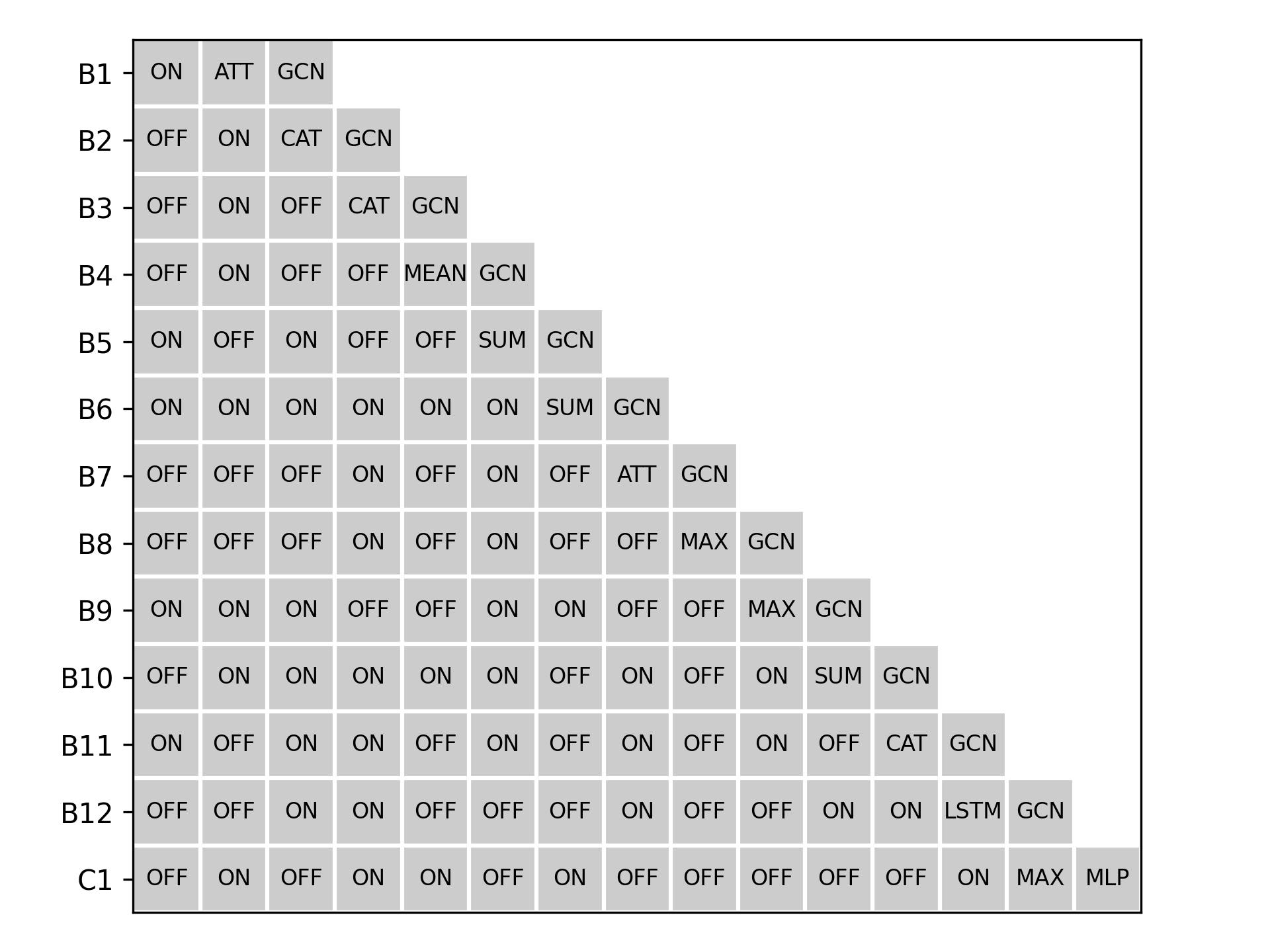
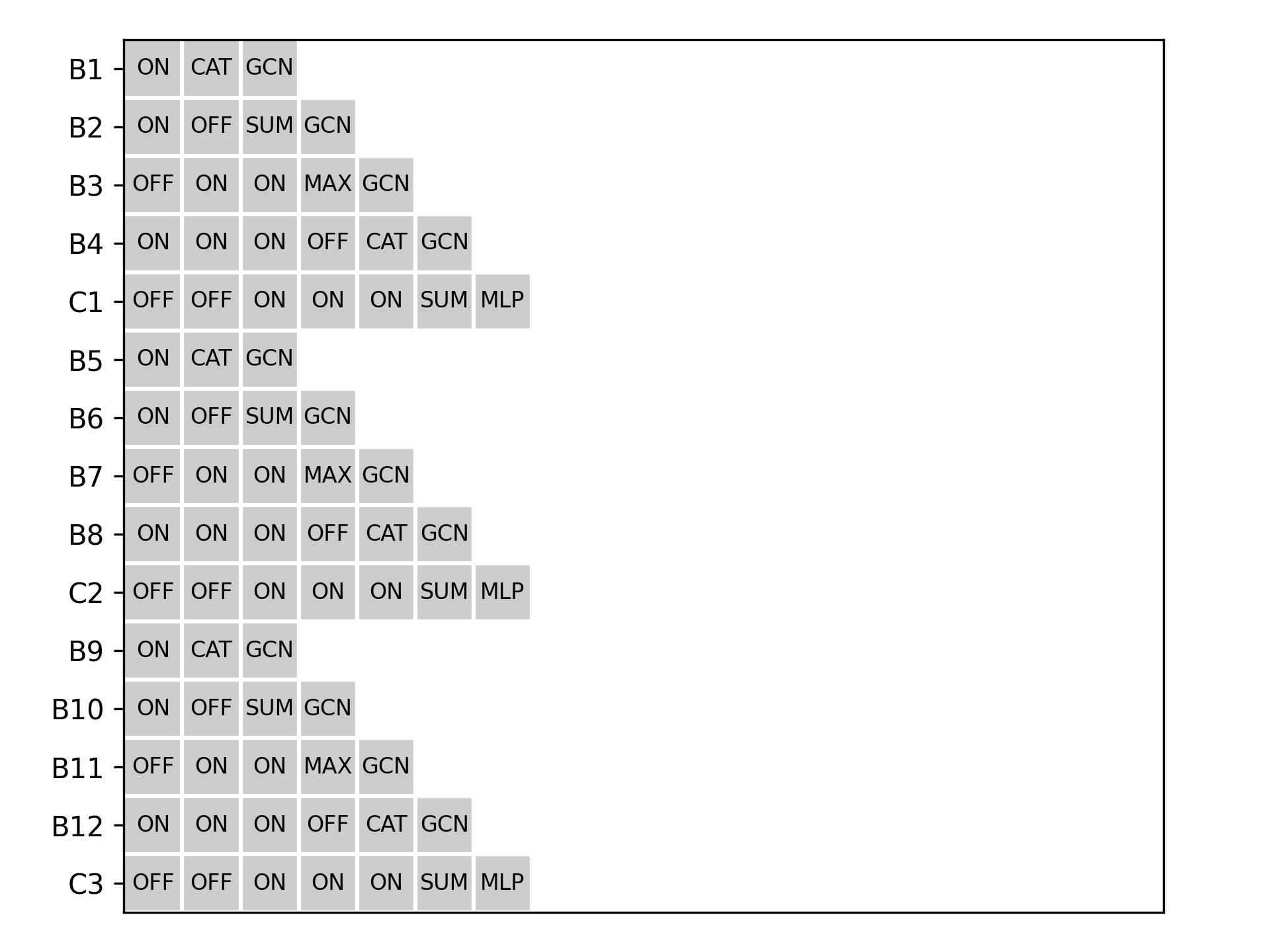
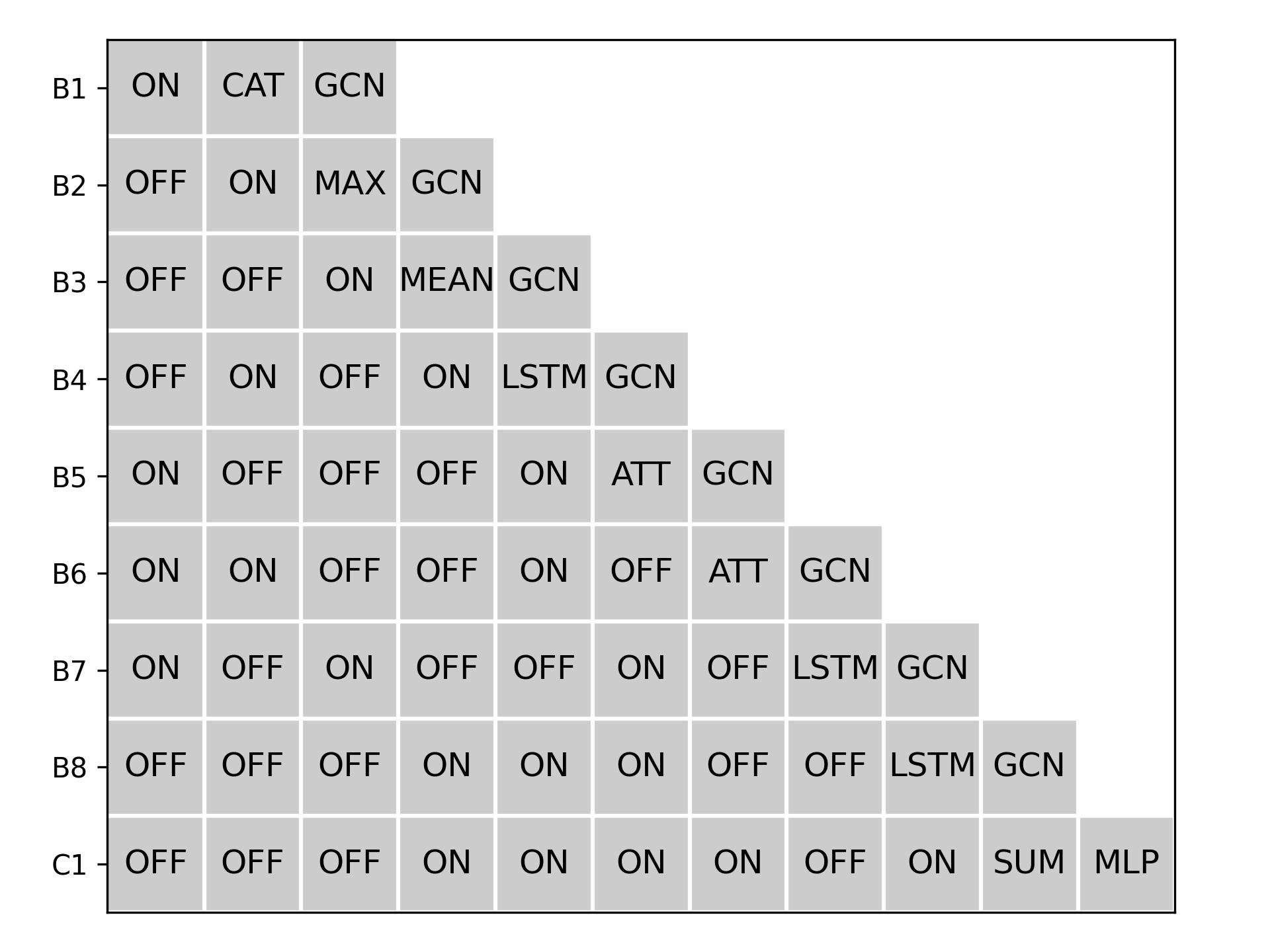
B.2. Searched GNNs

The the searched GNNs are provided in Fig. 11-15.

B.3. Ablation Study

B.3.1. The influence of different aggregation operations.

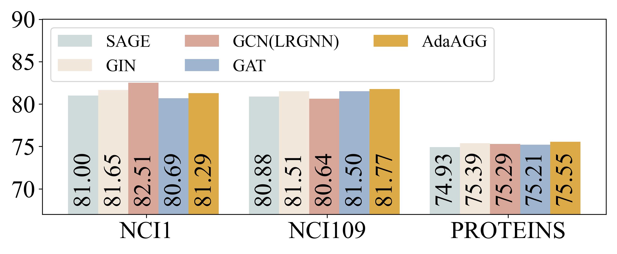
In this paper, we use the GCN operation to construct LRGNN. In this section, we employ different aggregation operations and evaluate their influence. As shown in Figure 9, compared with using fixed GCN operations in our paper, using the GIN operation will achieve higher performance, which is consistent with (Xu et al., 2019). Besides, we provide one variant AdaAGG which provide the aggregation design dimension additionally, i.e., $\{\texttt{SAGE},\texttt{GCN},\texttt{GIN},\texttt{GAT}\}$. It achieves higher performance than the proposed method LRGNN which uses fixed GCN operation. It indicates that the performance can be further improved in the future by adding more effective aggregation operations in the search space.

Figure 9. Evaluations on the basic aggregation operations. These methods are contructed with LRGNN-Full B12C1 variant and different aggregations.

B.3.2. The evaluation of search algorithm

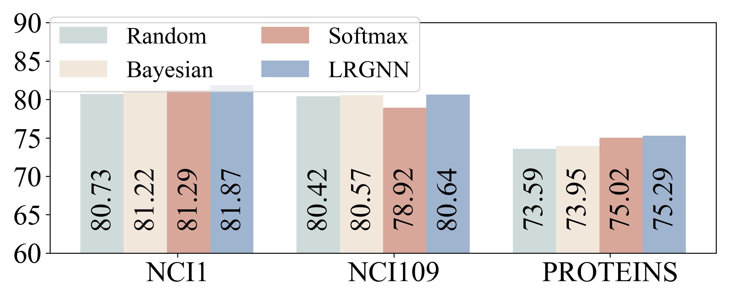
To make a fair comparison with LRGNN which adopts the Gumbel-Softmax function to relax the search space, we provide one baseline which uses the Softmax function as the relaxation function. We adopt the Random and Bayesian search algorithm in this section. These two methods have 100 search epochs in which one architecture is sampled from the search space and trained from scratch. We select the Top-1 architecture and tune this architecture, from which we obtained the final performance. As shown in Figure 10, the Random and Bayesian baselines cannot achieve higher performance than the differentiable methods on the designed search space. Besides, compared with these two methods, the relaxation function has smaller influences and could achieve comparable performance. Therefore, the presence of these differentiable search algorithm is essential for good performance, and the relaxation function matter less. This function can be further updated and could achieve considerable performance in expectation.

Figure 10. Evaluations on the search algorithm. We use LRGNN-Full B12C1 variant as an example. Softmax represent the differentiable algorithm with Softmax relaxation function, and our method employ the Gumbel-Softmax function instead.

Figure 11. The searched architectures on NCI1 dataset. Four variants from the left to right are the Full-B8C1, Full-B12C1, Repeat-B12C3, and Diverse-B12C3, respectively. In each row, the operations on each connections are showed. Besides, the merge operation and the aggregation operation are shown as well. In the post-processing operation, which denoted as “C” in this figure, use the MLP operation instead.

Figure 12. The searched architectures on NCI109 dataset.

Figure 13. The searched architectures on DD dataset.

Figure 14. The searched architectures on PROTEINS dataset.

Figure 15. The searched architectures on IMDB-BINARY dataset.

References

- (1)
- Abu-El-Haija et al. (2019) Sami Abu-El-Haija, Bryan Perozzi, Amol Kapoor, Nazanin Alipourfard, Kristina Lerman, Hrayr Harutyunyan, Greg Ver Steeg, and Aram Galstyan. 2019. Mixhop: Higher-order graph convolutional architectures via sparsified neighborhood mixing. In ICML. 21–29.
- Alon and Yahav (2021) Uri Alon and Eran Yahav. 2021. On the bottleneck of graph neural networks and its practical implications. ICLR (2021).
- Bianchi et al. (2020) Filippo Maria Bianchi, Daniele Grattarola, and Cesare Alippi. 2020. Spectral clustering with graph neural networks for graph pooling. In ICML. 874–883.
- Chen et al. (2020) Ming Chen, Zhewei Wei, Zengfeng Huang, Bolin Ding, and Yaliang Li. 2020. Simple and deep graph convolutional networks. In ICML. 1725–1735.
- Dobson and Doig (2003) Paul D Dobson and Andrew J Doig. 2003. Distinguishing enzyme structures from non-enzymes without alignments. Journal of molecular biology (JMB) 330, 4 (2003), 771–783.
- Dwivedi et al. (2022) Vijay Prakash Dwivedi, Ladislav Rampášek, Mikhail Galkin, Ali Parviz, Guy Wolf, Anh Tuan Luu, and Dominique Beaini. 2022. Long Range Graph Benchmark. arXiv preprint arXiv:2206.08164 (2022).
- Errica et al. (2020) Federico Errica, Marco Podda, Davide Bacciu, and Alessio Micheli. 2020. A fair comparison of graph neural networks for graph classification. ICLR.
- Feng et al. (2021) Guosheng Feng, Chunnan Wang, and Hongzhi Wang. 2021. Search For Deep Graph Neural Networks. arXiv preprint arXiv:2109.10047 (2021).
- Gao and Ji (2019) Hongyang Gao and Shuiwang Ji. 2019. Graph u-nets. ICML, 2083–2092.
- Gao et al. (2020) Yang Gao, Hong Yang, Peng Zhang, Chuan Zhou, and Yue Hu. 2020. Graphnas: Graph neural architecture search with reinforcement learning. In IJCAI.
- Gilmer et al. (2017) Justin Gilmer, Samuel S Schoenholz, Patrick F Riley, Oriol Vinyals, and George E Dahl. 2017. Neural Message Passing for Quantum Chemistry. In ICML. 1263–1272.
- Hamilton et al. (2017) Will Hamilton, Zhitao Ying, and Jure Leskovec. 2017. Inductive representation learning on large graphs. In NeurIPS. 1024–1034.
- He et al. (2016) Kaiming He, Xiangyu Zhang, Shaoqing Ren, and Jian Sun. 2016. Deep residual learning for image recognition. In CVPR. 770–778.
- Jain et al. (2021) Paras Jain, Zhanghao Wu, Matthew Wright, Azalia Mirhoseini, Joseph E Gonzalez, and Ion Stoica. 2021. Representing Long-Range Context for Graph Neural Networks with Global Attention. NeurIPS 34 (2021).
- Jiang and Balaprakash (2020) Shengli Jiang and Prasanna Balaprakash. 2020. Graph neural network architecture search for molecular property prediction. In 2020 IEEE International Conference on Big Data (Big Data). IEEE, 1346–1353.
- Kipf and Welling (2016) Thomas N Kipf and Max Welling. 2016. Semi-supervised classification with graph convolutional networks. ICLR (2016).
- Krizhevsky et al. (2012) Alex Krizhevsky, Ilya Sutskever, and Geoffrey E Hinton. 2012. Imagenet classification with deep convolutional neural networks. NIPS (2012).
- Lai et al. (2020) Kwei-Herng Lai, Daochen Zha, Kaixiong Zhou, and Xia Hu. 2020. Policy-GNN: Aggregation Optimization for Graph Neural Networks. In KDD. 461–471.
- Lee et al. (2019) Junhyun Lee, Inyeop Lee, and Jaewoo Kang. 2019. Self-Attention Graph Pooling. In ICML. 3734–3743.
- Li et al. (2019) Guohao Li, Matthias Muller, Ali Thabet, and Bernard Ghanem. 2019. Deepgcns: Can gcns go as deep as cnns?. In ICCV. 9267–9276.
- Li et al. (2018) Qimai Li, Zhichao Han, and Xiao-Ming Wu. 2018. Deeper insights into graph convolutional networks for semi-supervised learning. In AAAI.
- Li and King (2020) Yaoman Li and Irwin King. 2020. AutoGraph: Automated Graph Neural Network. In ICONIP. 189–201.
- Li et al. (2016) Yujia Li, Daniel Tarlow, Marc Brockschmidt, and Richard S. Zemel. 2016. Gated Graph Sequence Neural Networks. ICLR.
- Liu et al. (2019) Hanxiao Liu, Karen Simonyan, and Yiming Yang. 2019. DARTS: Differentiable architecture search. ICLR.
- Lukovnikov and Fischer (2021) Denis Lukovnikov and Asja Fischer. 2021. Improving Breadth-Wise Backpropagation in Graph Neural Networks Helps Learning Long-Range Dependencies.. In ICML. 7180–7191.
- Mesquita et al. (2020) Diego P. P. Mesquita, Amauri H. Souza Jr., and Samuel Kaski. 2020. Rethinking pooling in graph neural networks. In NeurIPS. 4800–4810.
- Paszke et al. (2019) Adam Paszke, Sam Gross, Francisco Massa, Adam Lerer, James Bradbury, Gregory Chanan, Trevor Killeen, Zeming Lin, Natalia Gimelshein, Luca Antiga, et al. 2019. Pytorch: An imperative style, high-performance deep learning library. In NeurIPS. 8026–8037.
- Pham et al. (2018) Hieu Pham, Melody Guan, Barret Zoph, Quoc Le, and Jeff Dean. 2018. Efficient Neural Architecture Search via Parameter Sharing. In ICML. 4092–4101.
- Pham et al. (2017) Trang Pham, Truyen Tran, Hoa Dam, and Svetha Venkatesh. 2017. Graph classification via deep learning with virtual nodes. arXiv preprint arXiv:1708.04357 (2017).
- Simonyan and Zisserman (2014) Karen Simonyan and Andrew Zisserman. 2014. Very deep convolutional networks for large-scale image recognition. arXiv preprint arXiv:1409.1556 (2014).
- Tan and Le (2019) Mingxing Tan and Quoc Le. 2019. Efficientnet: Rethinking model scaling for convolutional neural networks. In International conference on machine learning. PMLR, 6105–6114.
- Vaswani et al. (2017) Ashish Vaswani, Noam Shazeer, Niki Parmar, Jakob Uszkoreit, Llion Jones, Aidan N Gomez, Łukasz Kaiser, and Illia Polosukhin. 2017. Attention is all you need. NeurIPS 30 (2017).
- Veličković et al. (2018) Petar Veličković, Guillem Cucurull, Arantxa Casanova, Adriana Romero, Pietro Lio, and Yoshua Bengio. 2018. Graph attention networks. ICLR.
- Vinyals et al. (2016) Oriol Vinyals, Samy Bengio, and Manjunath Kudlur. 2016. Order Matters: Sequence to sequence for sets. ICLR (2016).
- Wale and Karypis (2006) N Wale and G Karypis. 2006. Comparison of Descriptor Spaces for Chemical Compound Retrieval and Classification. In ICDM. 678–689.
- Wang et al. (2022b) Xin Wang, Ziwei Zhang, and Wenwu Zhu. 2022b. Automated Graph Machine Learning: Approaches, Libraries and Directions. arXiv preprint arXiv:2201.01288 (2022).
- Wang et al. (2022d) Xu Wang, Huan Zhao, Lanning Wei, and Quanming Yao. 2022d. Graph Property Prediction on Open Graph Benchmark: A Winning Solution by Graph Neural Architecture Search. arXiv preprint arXiv:2207.06027 (2022).
- Wang et al. (2021b) Yiwei Wang, Wei Wang, Yuxuan Liang, Yujun Cai, and Bryan Hooi. 2021b. Curgraph: Curriculum learning for graph classification. In The WebConf. 1238–1248.
- Wang et al. (2021c) Yiwei Wang, Wei Wang, Yuxuan Liang, Yujun Cai, and Bryan Hooi. 2021c. Mixup for node and graph classification. In The WebConf. 3663–3674.
- Wang et al. (2021a) Zhili Wang, Shimin Di, and Lei Chen. 2021a. Autogel: An automated graph neural network with explicit link information. NeurIPS 34 (2021), 24509–24522.
- Wang et al. (2022a) Zhen Wang, Zhewei Wei, Yaliang Li, Weirui Kuang, and Bolin Ding. 2022a. Graph Neural Networks with Node-wise Architecture. In Proceedings of the 28th ACM SIGKDD Conference on Knowledge Discovery and Data Mining. 1949–1958.
- Wang et al. (2022c) Zhenyi Wang, Huan Zhao, and Chuan Shi. 2022c. Profiling the Design Space for Graph Neural Networks based Collaborative Filtering. In WSDM. 1109–1119.
- Wei et al. (2022) Lanning Wei, Huan Zhao, and Zhiqiang He. 2022. Designing the Topology of Graph Neural Networks: A Novel Feature Fusion Perspective. In The WebConf. 1381–1391.
- Wei et al. (2021) Lanning Wei, Huan Zhao, Quanming Yao, and Zhiqiang He. 2021. Pooling architecture search for graph classification. In CIKM. 2091–2100.
- Xie et al. (2018) Sirui Xie, Hehui Zheng, Chunxiao Liu, and Liang Lin. 2018. SNAS: stochastic neural architecture search. ICLR (2018).
- Xu et al. (2019) Keyulu Xu, Weihua Hu, Jure Leskovec, and Stefanie Jegelka. 2019. How powerful are graph neural networks? ICLR.
- Xu et al. (2018) Keyulu Xu, Chengtao Li, Yonglong Tian, Tomohiro Sonobe, Ken-ichi Kawarabayashi, and Stefanie Jegelka. 2018. Representation learning on graphs with jumping knowledge networks. In ICML. 5453–5462.
- Yanardag and Vishwanathan (2015) Pinar Yanardag and SVN Vishwanathan. 2015. Deep graph kernels. In KDD. 1365–1374.
- Ying et al. (2021) Chengxuan Ying, Tianle Cai, Shengjie Luo, Shuxin Zheng, Guolin Ke, Di He, Yanming Shen, and Tie-Yan Liu. 2021. Do transformers really perform badly for graph representation? NeurIPS 34 (2021), 28877–28888.
- Ying et al. (2018) Zhitao Ying, Jiaxuan You, Christopher Morris, Xiang Ren, Will Hamilton, and Jure Leskovec. 2018. Hierarchical graph representation learning with differentiable pooling. In NeurIPS. 4800–4810.
- Yoo et al. (2022) Jaemin Yoo, Sooyeon Shim, and U Kang. 2022. Model-agnostic augmentation for accurate graph classification. In The WebConf. 1281–1291.
- You et al. (2020) Jiaxuan You, Rex Ying, and Jure Leskovec. 2020. Design Space for Graph Neural Networks. In NeurIPS.
- Yuan and Ji (2020) Hao Yuan and Shuiwang Ji. 2020. StructPool: Structured graph pooling via conditional random fields. ICLR (2020).
- Zhang et al. (2018) Muhan Zhang, Zhicheng Cui, Marion Neumann, and Yixin Chen. 2018. An end-to-end deep learning architecture for graph classification. In AAAI.
- Zhang et al. (2020) Yufeng Zhang, Xueli Yu, Zeyu Cui, Shu Wu, Zhongzhen Wen, and Liang Wang. 2020. Every document owns its structure: Inductive text classification via graph neural networks. In ACL. Association for Computational Linguistics, 334–339.
- Zhang et al. (2021) Ziwei Zhang, Xin Wang, and Wenwu Zhu. 2021. Automated Machine Learning on Graphs: A Survey. arXiv preprint arXiv:2103.00742 (2021).
- Zhao et al. (2020) Huan Zhao, Lanning Wei, and Quanming Yao. 2020. Simplifying Architecture Search for Graph Neural Network.
- Zhao et al. (2021) Huan Zhao, Quanming Yao, and Weiwei Tu. 2021. Search to aggregate neighborhood for graph neural network. In ICDE.