Towards Efficient Alternating Current Optimal Power Flow Analysis on Graphical Processing Units

Abstract

We present a solution of sparse alternating current optimal power flow (ACOPF) analysis on graphical processing unit (GPU). In particular, we discuss the performance bottlenecks and detail our efforts to accelerate the linear solver, a core component of ACOPF that dominates the computational time. ACOPF analyses of two large-scale systems, synthetic Northeast (25,000 buses) and Eastern (70,000 buses) U.S. grids [1], on GPU show promising speed-up compared to analyses on central processing unit (CPU) using a state-of-the-art solver. To our knowledge, this is the first result demonstrating a significant acceleration of sparse ACOPF on GPUs.

I Introduction

The electric power grid is undergoing a massive transformation with the influx of new technologies, processes, and digitization to provide cleaner, smarter, affordable, and equitable electricity to everyone. Yet, at the same time, the grid is witnessing an unprecedented increase in threats caused by climate change and cyber attacks. Blackouts caused in California due to heat waves, outages due to hurricanes in Florida and Puerto Rico, are some recent examples of massive power disruptions affecting millions of lives. Operating the grid under such “dark sky” events and, in general, “intermittent sky” days with uncertain renewable forecasts, remains an ever-increasing challenge. Accurate and fast wide area analysis tools provide critical aid to grid operators and planners, as they make decisions. However, with greater fidelity comes greater computational complexity.

Heterogeneous computing, such as combining CPUs with hardware accelerators, is becoming a dominant paradigm in the computing landscape. Spurred by demand from the video gaming industry, artificial intelligence and computer vision applications, GPUs are the most prevalent hardware accelerators today. GPUs deliver high computational power at low cost through massive fine-grain parallelism.

The challenge for using GPUs arises from their single-instruction multiple-data (SIMD) architecture that imposes modeling and solver constraints. The SIMD architecture is suitable for porting legacy CPU-based dense vector and matrix operations. Legacy sparse operations, which are used in current state-of-the-art ACOPF analysis [2] cannot be recast in SIMD terms without additional mathematical considerations.

In our prior work [3], we discussed solving ACOPF [2, 4] on GPUs with a dense solver, by compressing the sparse formulation that naturally arises from power systems. Earlier, an approach for solving convex ACOPF problems using fully dense linear algebra and Cholesky solver was proposed in [5]. However, the computational complexity of dense linear solvers is $O(N^{3})$ and their memory complexity is $O(N^{2})$, where $N$ is the number of linear equations. For larger grid models, all performance gains on GPU are offset by a cubic increase in computational cost and a quadratic increase in memory.

Here, we present our results on solving sparse ACOPF on GPUs. In particular, we detail our efforts on accelerating the linear solver, a core component of ACOPF that dominates the computational cost [6]. This exploration is motivated by our recent efforts on sparse linear solvers for ACOPF problems [7, 8], as well as recent investigations of dynamic phasor simulations [9, 10], power flow [11, 12], and batched power flow simulations [13, 14] on GPUs.

The main contributions of this paper are:

• First reported meaningful acceleration of ACOPF on GPUs, using our sparse linear solver, demonstrated on large interconnection-level grid models and reproducible using the open-source ExaGO^TM package (Sec. III).

• Performance analysis of ACOPF on CPUs (Sec. II) and GPUs (Sec. III) with key bottlenecks identified.

• Performance projections and limitations of current technology and identifying research needed to achieve even better acceleration on GPUs (Sec. IV and V).

II State of The Art Methods for Alternating Current Optimal Power Flow Analysis

ACOPF falls in the category of nonlinear nonconvex optimization problems. In compact mathematical form it can be formulated as

$$\underset{x}{\min} ~{}F(x)$$ (1)

s.t. $$g(x)=0$$ (2)

$$h^{-} \leq h(x)\leq h^{+}$$ (3)

$$x^{-} \leq x\leq x^{+}$$ (4)

where $F(x)$ is a scalar function defining the optimization objective, typically the total cost of generation; $x$ is the vector of optimization variables, such as generator power outputs; vectors $x^{-},x^{+}$ define variable bounds, e.g. resource capacity limits; vector function $g(x)$ defines equality constraints, like power balance; and vector function $h(x)$ defines security constraints with security limits given by vectors $h^{-},h^{+}$. The reader is referred to [15, 2] for comprehensive details on the ACOPF formulation.

The optimization problem (1)-(4) is typically solved in an iterative manner using an interior-point method [16]. To keep our presentation streamlined and without loss of generality, we rewrite (1)-(4) in a more compact form

$$\underset{y}{\min}~{} f(y)$$ (5)

s.t. $$c(y)=0$$ (6)

$$y\geq 0$$ (7)

Here we convert (3) to equality constraints by adding slack variables $s^{\prime},s^{\prime\prime}\geq 0$ satisfying $h(x)-h^{-}-s^{\prime}$ and $h(x)-h^{+}+s^{\prime\prime}$. Bounds (4) are expressed in form (7) by introducing variables $x^{\prime},x^{\prime\prime}\geq 0$ such that $x-x^{-}=x^{\prime}$ and $x^{+}-x=x^{\prime\prime}$. In the compact form, the vector of optimization primal variables is $y=(x^{\prime},x^{\prime\prime},s^{\prime},s^{\prime\prime})\in\mathbb{R}^{n}$ and $f:\mathbb{R}^{n}\to\mathbb{R}$ is the scalar objective function $F(x)$ expressed in space of primal variables $y$. All constraints are formulated in $c:\mathbb{R}^{n}\to\mathbb{R}^{m}$, where $m$ is the number of equality and inequality constraints.

To enforce variable bounds, the objective function (5) is augmented with barrier functions as

$$\phi(y)=f(y)+\mu\sum_{i=1}^{n}\ln y_{i}.$$ (8)

The solution to the barrier subproblem then can be obtained by solving the nonlinear equations

$$\nabla{f(y)}+\nabla{c(y)}\lambda-z =0,$$ (9)

$$c(y) =0,$$ (10)

$$Yz-\mu e =0$$ (11)

where $J\equiv\nabla{c(y)}$ is the $m\times n$ constraint Jacobian matrix, $\lambda\in\mathbb{R}^{m}$ and $z\in\mathbb{R}^{n}$ are vectors of Lagrange multipliers for equality (10) and bound constraints (11), respectively, $Y\equiv\text{diag}(y)$, and $e\in\mathbb{R}^{n}$ is a vector of ones.

The barrier subproblem (9)-(11) is solved using a Newton method, and the solution to the original optimization problem is obtained by a continuation algorithm setting $\mu\to 0$. As it searches for the optimal solution, the interior-point method solves a sequence of linearized systems $K_{k}\Delta x_{k}=r_{k}$, $k=1,2,\dots,M$ of Karush-Kuhn-Tucker (KKT) type. A typical implementation of an interior-point method eliminates $z$ from the linearized version of (9)-(11) by block-Gaussian elimination to obtain smaller symmetric system

$$\overbrace{\begin{bmatrix}H+D_{y}&J\\ J^{T}&0\end{bmatrix}}^{K_{k}}\overbrace{\begin{bmatrix}\Delta y\\ \Delta\lambda\end{bmatrix}}^{\Delta x_{k}}=\overbrace{\begin{bmatrix}r_{y}\\ r_{\lambda}\end{bmatrix}}^{r_{k}},$$ (12)

where index $k$ denotes the optimization solver iteration (including continuation step in $\mu$ and Newton iterations), $K_{k}$ is a system (KKT) matrix, vector $\Delta x_{k}$ is a search direction for the primal and dual variables, and $r_{k}$ is derived from the residual vector for (9)-(11) evaluated at the current value of the primal and dual variables. The Hessian

$$H\equiv\nabla^{2}f(y)+\sum_{i=1}^{m}\lambda_{i}\nabla^{2}c_{i}(y),$$

is a sparse symmetric $n\times n$ matrix and $D_{y}\equiv\mu Y^{-2}$ is a diagonal $n\times n$ matrix. For more details on interior-point methods implementations we refer reader to [16].

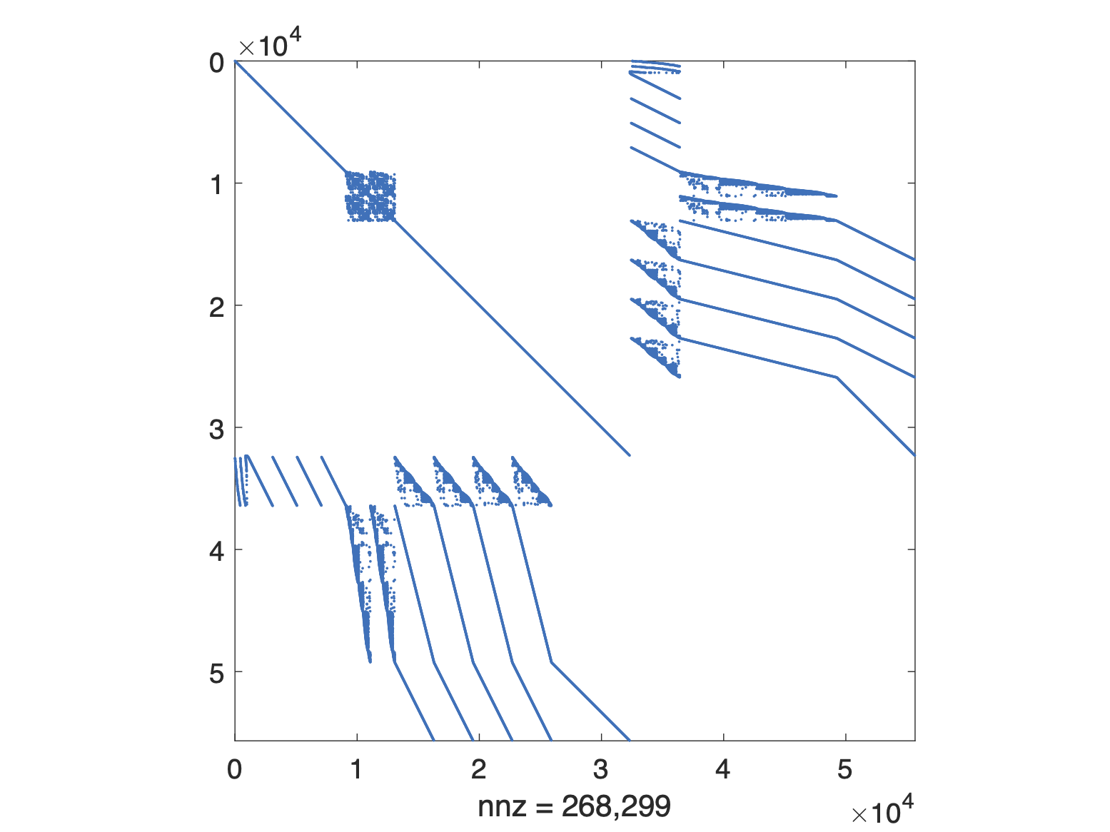
Matrices $K_{k}$ in (12) are sparse symmetric indefinite. All $K_{k}$ have the same sparsity pattern, a property that can be exploited by a solver. Characteristic for ACOPF is that $K_{k}$ generated in the analysis are very sparse with an irregular non-zero pattern without dense blocks [17]. One such example is shown in Figure 1.

Figure 1: Sparsity pattern of KKT matrix obtained in ACOPF analysis for 2000-bus Texas grid model.

When the barrier parameter $\mu=0$, the matrix in (12) is singular. The continuation algorithm driving $\mu\to 0$ therefore needs to exit when the solution to the augmented system is close enough to the solution of the original system, but before (12) becomes too ill-conditioned. Typically, KKT matrices are characterized by extremely high condition numbers ($>10^{16}$), which means that solving these systems in a naive way (e.g. without pivoting and equilibration) would result in solutions with error exceeding computer floating point double precision.

Only a few linear solvers have been effective for this type of problems. These solvers are typically sparse direct solvers based on $\text{LDL}^{\text{T}}$ or $LU$ decomposition [18]. State-of-the art approaches usually employ KLU (for non-symmetric matrices) [19, 10] or MA57 [20].

A sparse direct solver typically computes the solution to a linear system in three stages: ($i$) an analysis stage, where the system is equilibrated, column and row permutations are set, pivot order is established and the non-zero pattern of the factors is chosen; ($ii$) a numerical factorization stage, in which matrix factors are computed and ($iii$) a solution stage, in which the factors computed in the previous stage are used for forward and backward triangular solves. Some solvers follow the third stage by iterative refinement [21]. The first stage is considered to be more expensive than others, but if the matrix non-zero pattern does not change between the systems, as in (12), the analysis can be executed once and the results reused for all $K_{k}$ [10, 12]. The numerical factorization stage typically requires pivoting for the computation to remain stable. Pivoting changes the sparsity pattern of $L$ and $U$ factors and in some cases may even require memory reallocation. Therefore, while changes in the pivot sequence may not be a concern on CPUs, they degrade performance on GPUs as we describe in Sec. III.

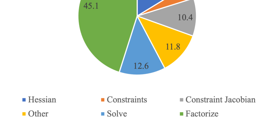
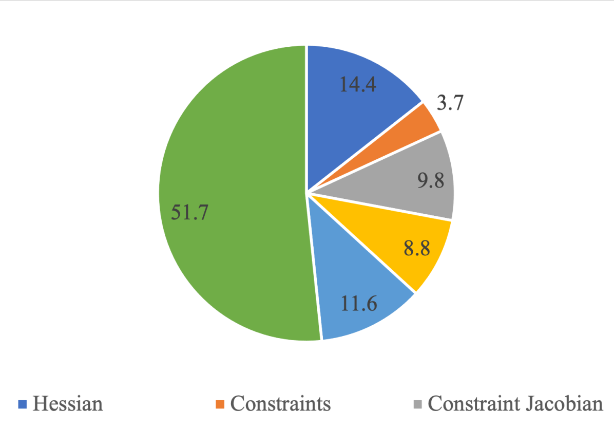
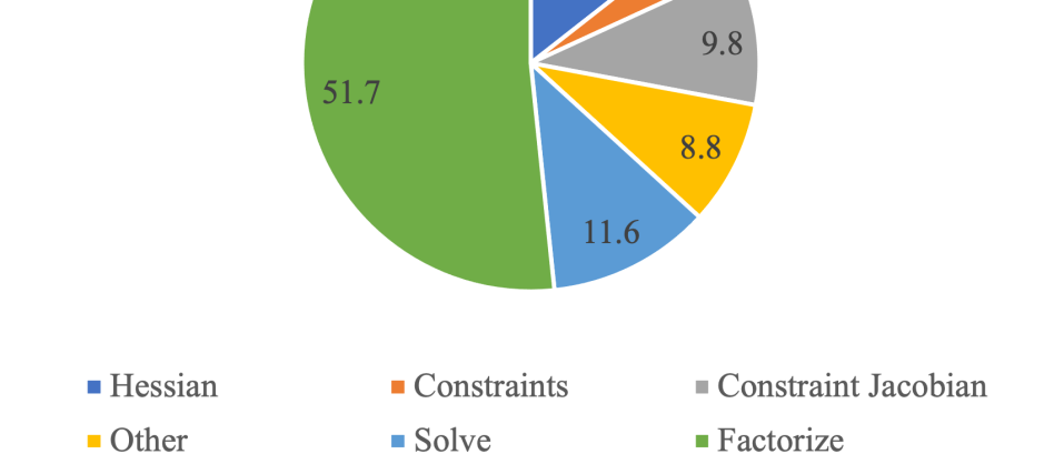
For ACOPF problems, more than a half of the overall computational cost is typically spent solving the KKT linear system. Within that, the largest cost is in matrix factorization (symbolic and numeric factorization) and to a lesser degree in triangular solves (backward-forward substitution). Other significant items are evaluation of derivative matrices – constraint Jacobian $J$, and Hessian matrix $H$. We illustrate that in Fig. 2 where we show computational cost breakdown for ACOPF for 25,000-bus model of Northeast U.S. grid and 70,000-bus model of Eastern U.S. grid, respectively. Table I provides a description of the two synthetic grids evaluated.

(a) Northeast U.S. grid

(b) Eastern U.S. grid

Figure 2: Computational cost of ACOPF broken down by solver functions. Linear solver functions (matrix factorization and triangular solve) contribute to 60% of the overall ACOPF compute time.

TABLE I: Description of synthetic grid models from [1] used in performance analysis. The specifics of the linear system (12) for each of these models are given in terms of the matrix $K_{k}$ size (N) and number of non-zeros (nnz).

Grid	Buses	Gen’s	Branches	N	nnz
Northeast U.S	25,000	4,834	32,230	107,558	1,191,152
Eastern U.S.	70,000	10,390	88,270	296,214	3,228,456

The analysis has been performed using the ExaGO^TM package [22] with the HiOp optimization engine [23] and the MA57 linear solver. Numerical matrix factorization takes roughly half of the total compute time in ACOPF, while the triangular solve takes another 12%. Model evaluation operations take about 30% of the total compute time. All other operations (evaluation of the objective, objective gradient, infeasibility norm, etc.) in ACOPF take less than 10% of the overall time. Achieving any speedup largely depends on how effectively the KKT linear system can be solved on a GPU.

III Computing with graphical processing units

There has been a substantial effort in the scientific community devoted towards using GPU acceleration to speed up sparse direct linear solvers, and the available software usually has at least some GPU capabilities. However, solving the linear systems described herein on GPUs is particularly challenging: ($i$) Due to irregular and very sparse nature of power systems, the underlying linear problems do not have a structure that traditional multifrontal [24] and supernodal [25] approaches can use to form dense blocks where SIMD operations can be performed. ($ii$) The underlying linear problems are ill-conditioned and require pivoting for numerical factorization stability. Pivoting degrades performance on GPUs because of conditional branching and considerable data movement [13].

In [7], we identified and tested several GPU accelerated sparse direct solvers and concluded that none of them was faster than MA57, especially for the largest test cases. These solvers only offload a part of the computations (e.g., matrix-matrix products or triangular solves) to the GPU, while the rest of the computation happens on the CPU. This results in a substantial overhead associated with allocating and freeing small chunks of GPU memory and copying the data to and from the device. For our test cases, we also observed that factorization on the GPU was particularly expensive.

We use a refactorization approach to solve (12) on GPU (see Algorithm 1, $M$ is the total number of systems to solve, this number depends on optimization solver settings, typically in the order of 100s). A similar approach was successfully used for dynamic phasor [10, 9] and power flow [12] simulations but not for ACOPF. Our approach is the first we are aware of, where the sparse linear solvers in ACOPF analysis were accelerated using GPUs and outperformed state-of-the-art CPU solvers. We replace the MA57 solver in our software stack with a solver we implemented using KLU and NVIDIA’s cuSolver libraries. We factorize the first system on the CPU using KLU, set the patterns of $L$ and $U$, and compute the permutation vectors. We also evaluated cuSolver’s methods for setting the patterns of $L$ and $U$, but found KLU to perform better. Once computed, we keep the sparsity pattern of the factors the same for the rest of the computation. The non-zero structure of the factors and the permutation vectors are then copied to the GPU and passed to cuSolver. The refactorization is set up, and each subsequent system is solved using GPU refactorization, without a need for pivoting, which is prohibitively expensive on GPUs.

Algorithm 1 Refactorization Solution Strategy: KLU + cuSolverGLU

Input: Sequence of linear systems $K_{k}x_{k}=b_{k}$, $k=1,2,\ldots,M$
      Output: Sequence of solution vectors $x_{k}$

1:Use KLU to solve $Ax_{1}=b_{1}$

2:Extract symbolic factorization and permutation vectors. $\triangleleft$ Using klu_extract, returns L,U in CSC format

3:Convert CSC to combined L+U CSR object. $\triangleleft$ Up to here, computed on the CPU

4:Setup cuSolverGLU$\triangleleft$ GPU computation starts

5:for $k=2,\ldots,M$ do $\triangleleft$ $M$ is the total number of linear systems

6:     Update factorization object using new values from $K_{k}$.     $\triangleleft$ Using cuSolverGLU function

7:     Refactor.

8:     Perform triangular solve for $b_{k}$. $\triangleleft$ Always followed by built-in iterative refinement

9:end for

Using this method all data movement and mapping is done only once on the CPU while the subsequent computations are implemented in terms of SIMD operations on GPU. The tradeoff is that the refactorization approach produces a lower quality solution, so the solve stage may need to be followed by an iterative refinement to recover the accuracy needed by the optimization method.

Two refactorization interfaces were tested: cuSolverGLU and cuSolverRf. cuSolverGLU is an undocumented (but publicly available) part of the cuSolver library. It is generally faster than cuSolverRf, more numerically stable and comes with built-in iterative refinement. We used cuSolverGLU for all the results shown in this paper. cuSolverGLU requires a combined $L+U$ storage of the factors in CSR format hence we needed to perform a format conversion after using KLU, which operates on matrices in CSC format.

A great advantage of cuSolver refactorization is that the user is allowed to provide the non-zero patterns of their own $L$ and $U$ factors and the permutation vectors; the factors can come from any $LU$ solver (as long as the data format is correct) and cuSolver will carry on the computation on the GPU for the next systems in the sequence.

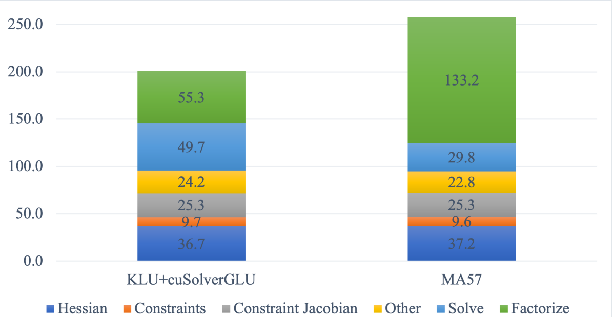
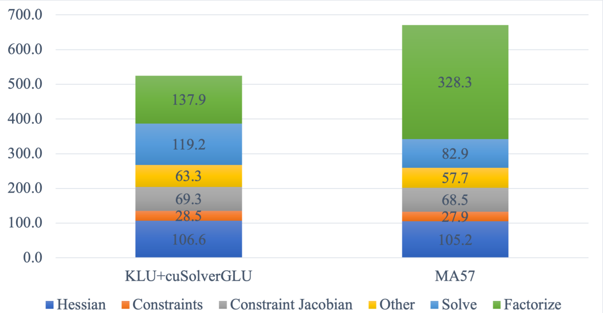
Since the optimization solver typically calls the linear solver hundreds of times, the cost of one linear solve performed on CPU can be amortized over subsequent iterations. In Fig. 3 and Table II, we show the computational speedup obtained using this approach. The figure shows the average cost per optimization solver iteration, including the amortized cost of one-time factorization with KLU. The numerical experiments were conducted with an IBM Power 9 CPU and an NVIDIA V100 GPU, which has 16 GB of high bandwidth memory and approximately 7 TF of double precision peak performance.

(a) Northeast U.S. grid

(b) Eastern U.S. grid

Figure 3: Comparison of the computational cost (average time per iteration in milliseconds) between CPU and GPU with a breakdown in terms of most expensive operations. Model evaluation time is the same in both test cases since only linear solver is GPU accelerated.

TABLE II: Comparison of total run times for ACOPF show 30% speedup when using sparse linear solver on GPU

Northeast U.S. grid
Linear solver used	KLU+cuSolver	MA57	Speedup
Total time (s)	116.0	152.1	1.3
Number of iterations	547	529	-
Eastern U.S. grid
Linear solver used	KLU+cuSolver	MA57	Speedup
Total time (s)	146.7	196.4	1.3
Number of iterations	263	263	-

The overall speedup is entirely due to acceleration of the numerical factorization. Including the cost of initial KLU factorization, we obtain an average speedup of $2.4\times$ for the factorization and $1.3\times$ overall compared to MA57 benchmark on CPU. Somewhat surprisingly, we find that triangular solve is 30-40% slower on GPU. This is likely due to a suboptimal iterative refinement embedded in cuSolverGLU triangular solver function. We also note there is a slight increase in “other” computational cost when using GPUs. This increase is mostly due to the overhead of the CUDA API, including the cost of launching GPU kernels. Other parts of the computation were not GPU-accelerated and have the same cost, approximately, in both test configurations. Data movement between CPU and GPU during the solution process is less than 2% of GPU time.

The solver requires little memory on the GPU (1.1 GB and 2.9 GB for the 25,000-bus model of the Northeast U.S. grid and the 70,000-bus model of Eastern U.S. grid, respectively). This is in stark contrast with the implementation in [3], which requires 21 GB of GPU memory for the smaller 10,000-bus model of Western U.S. grid.

IV Projected Performance Improvement with Available Technology

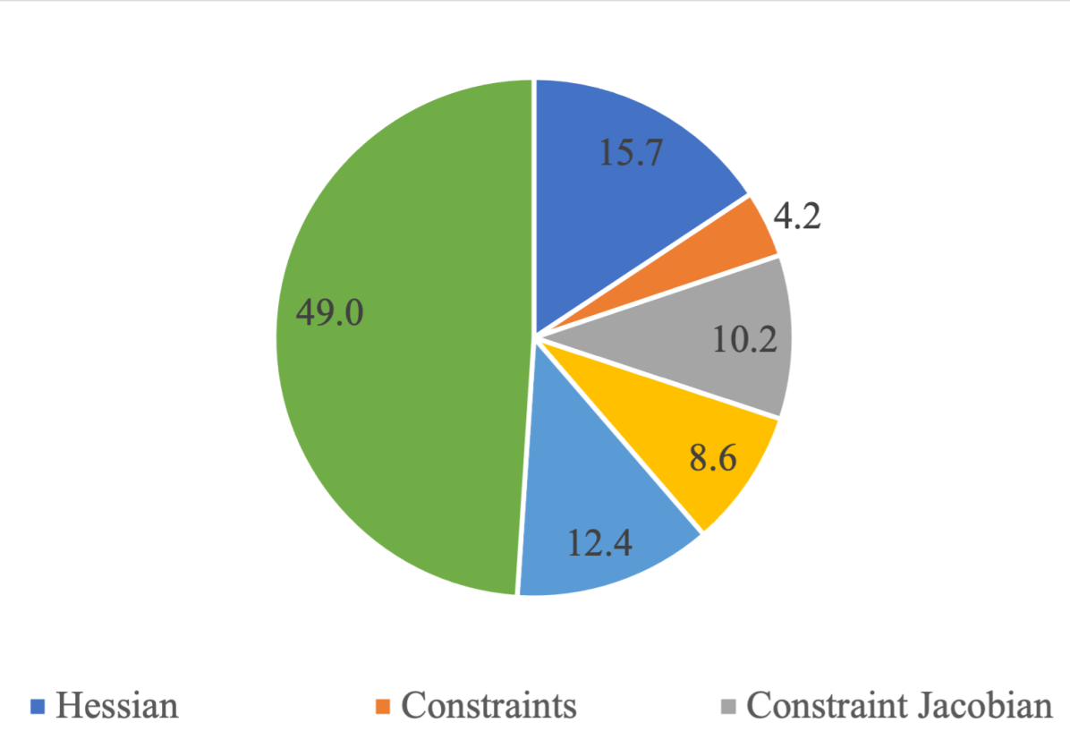
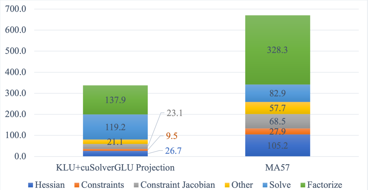
The entire performance improvement for ACOPF is due to acceleration of matrix factorization on GPU (Figure 3). Results in [3] show that the model evaluation could be GPU-accelerated, as well. We can therefore make projections for further performance improvements. We conservatively anticipate a $4\times$ speedup for the sparse Hessian evaluation on GPU and $3\times$ for constraints, constraint Jacobians and other model components. In [3], speedup of $2$-$3\times$ was achieved on vector kernels and more than $15\times$ on dense matrix kernels for the largest grid evaluated (2,000-bus Texas grid model). While memory access is more efficient when evaluating dense matrix elements, we nevertheless believe it is safe to expect at least $4\times$ speedup for sparse matrix evaluation, especially for the large use cases we consider. Fig. 4 illustrates the projected performance for the Eastern U.S. grid ($2\times$ speedup on the GPU) if the model evaluation were performed on the GPU.

Figure 4: A conservative projection of speedup for ACOPF analysis with technology already available in ExaGO^TM and HiOp libraries shows $2\times$ speedup for the Eastern U.S. grid.

V Conclusions and Next steps

We eliminated the main bottleneck for efficient ACOPF analysis on GPU by accelerating sparse matrix factorization by $2.4\times$ compared to an MA57 baseline on CPU. With only the linear solver accelerated, we get a 30% overall speedup for ACOPF analysis. We also show it is feasible to accelerate the entire analysis by at least $2\times$ with technology available today.

The GPU profiling result clearly show that the next bottleneck of the entire linear system solution pathway is now the GPU triangular solve. We believe that significant improvement is possible by using a more efficient and configurable iterative refinement than the one embedded in the cuSolverGLU library. Triangular solves can also be approximated by Jacobi or Gauss-Seidel iteration with very promising performance results [26], but our investigation on that topic is at an early stage.

The ACOPF matrices exhibit what is known as a saddle-point structure in the literature. A specialized, GPU-ready solver, which exploits this structure was developed in [8]. This solver performs triangular solve on smaller matrices, and early (standalone) results show an impressive speedup over MA57. In the future, we plan to integrate it with our software stack and evaluate its performance.

References

- [1] A. B. Birchfield, T. Xu, K. M. Gegner, K. S. Shetye, and T. J. Overbye, “Grid structural characteristics as validation criteria for synthetic networks,” IEEE Transactions on Power Systems, vol. 32, no. 4, pp. 3258–3265, 2017.
- [2] R. P. O’Neill, A. Castillo, and M. B. Cain, “The IV formulation and linear approximations of the AC optimal power flow problem (OPF Paper 2),” FERC Staff Technical Paper, no. December, pp. 1–18, 2012. [Online]. Available: http://www.ferc.gov/industries/electric/indus-act/market-planning/opf-papers/acopf-2-iv-linearization.pdf
- [3] S. Abhyankar, S. Peles, R. Rutherford, and A. Mancinelli, “Evaluation of AC optimal power flow on graphical processing units,” in 2021 IEEE Power & Energy Society General Meeting (PESGM), 2021, pp. 01–05.
- [4] S. Frank, S. Rebennack et al., “A Primer on Optimal Power Flow: Theory, Formulation, and Practical Examples,” Colorado School of Mines, Tech. Rep. 14, 2012.
- [5] L. Rakai and W. Rosehart, “Gpu-accelerated solutions to optimal power flow problems,” in 2014 47th Hawaii International Conference on System Sciences, 2014, pp. 2511–2516.
- [6] X. Su, C. He, T. Liu, and L. Wu, “Full parallel power flow solution: A GPU-CPU-based vectorization parallelization and sparse techniques for Newton–Raphson implementation,” IEEE Transactions on Smart Grid, vol. 11, no. 3, pp. 1833–1844, 2019.
- [7] K. Świrydowicz, E. Darve, W. Jones, J. Maack, S. Regev, M. A. Saunders, S. J. Thomas, and S. Peleš, “Linear solvers for power grid optimization problems: a review of GPU-accelerated linear solvers,” Parallel Computing, vol. 111, p. 102870, 2022.
- [8] S. Regev, N.-Y. Chiang, E. Darve, C. G. Petra, M. A. Saunders, K. Świrydowicz, and S. Peleš, “HyKKT: a hybrid direct-iterative method for solving KKT linear systems,” Optimization Methods and Software, pp. 1–24, 2022.
- [9] J. Dinkelbach, L. Schumacher, L. Razik, A. Benigni, and A. Monti, “Factorisation path based refactorisation for high-performance LU decomposition in real-time power system simulation,” Energies, vol. 14, no. 23, p. 7989, 2021.
- [10] L. Razik, L. Schumacher, A. Monti, A. Guironnet, and G. Bureau, “A comparative analysis of LU decomposition methods for power system simulations,” in 2019 IEEE Milan PowerTech. IEEE, 2019, pp. 1–6.
- [11] D. Ablakovic, I. Dzafic, and S. Kecici, “Parallelization of radial three-phase distribution power flow using GPU,” in 2012 3rd IEEE PES Innovative Smart Grid Technologies Europe (ISGT Europe), 2012, pp. 1–7.
- [12] M. D’orto, S. Sjöblom, L. S. Chien, L. Axner, and J. Gong, “Comparing different approaches for solving large scale power-flow problems with the Newton-Raphson method,” IEEE Access, vol. 9, pp. 56 604–56 615, 2021.
- [13] G. Zhou, R. Bo, L. Chien, X. Zhang, F. Shi, C. Xu, and Y. Feng, “GPU-based batch lu-factorization solver for concurrent analysis of massive power flows,” IEEE Transactions on Power Systems, vol. 32, no. 6, pp. 4975–4977, 2017.
- [14] G. Zhou, R. Bo, L. Chien, X. Zhang, S. Yang, and D. Su, “GPU-accelerated algorithm for online probabilistic power flow,” IEEE Transactions on Power Systems, vol. 33, no. 1, pp. 1132–1135, 2018.
- [15] R. D. Zimmerman, C. E. Murillo-Sánchez, and R. J. Thomas, “MATPOWER: Steady-state operations, planning, and analysis tools for power systems research and education,” IEEE Transactions on Power Systems, vol. 26, no. 1, pp. 12–19, 2011.
- [16] A. Wächter and L. T. Biegler, “On the implementation of an interior-point filter line-search algorithm for large-scale nonlinear programming,” Mathematical programming, vol. 106, no. 1, pp. 25–57, 2006.
- [17] L. R. de Araujo, D. R. R. Penido, J. L. R. Pereira, and S. Carneiro, “A sparse linear systems implementation for electric power systems solution algorithms,” Journal of Control, Automation and Electrical Systems, vol. 24, no. 4, pp. 504–512, Aug 2013.
- [18] G. H. Golub and C. F. Van Loan, Matrix computations. JHU press, 2013.
- [19] T. A. Davis and E. Palamadai Natarajan, “Algorithm 907: KLU, a direct sparse solver for circuit simulation problems,” ACM Transactions on Mathematical Software (TOMS), vol. 37, no. 3, pp. 1–17, 2010.
- [20] I. S. Duff, “MA57—a code for the solution of sparse symmetric definite and indefinite systems,” ACM Transactions on Mathematical Software (TOMS), vol. 30, no. 2, pp. 118–144, 2004.
- [21] R. D. Skeel, “Iterative refinement implies numerical stability for Gaussian elimination,” Mathematics of computation, vol. 35, no. 151, pp. 817–832, 1980.
- [22] S. Abhyankar, S. Peles, A. Mancinelli, R. Rutherford, and B. Palmer, “Exascale grid optimization toolkit,” 2020. [Online]. Available: https://https://gitlab.pnnl.gov/exasgd/frameworks/exago
- [23] C. G. Petra, N. Chiang, and J. Wang, “HiOp – User Guide,” Center for Applied Scientific Computing, Lawrence Livermore National Laboratory, Tech. Rep. LLNL-SM-743591, 2018.
- [24] I. S. Duff and J. K. Reid, “The multifrontal solution of indefinite sparse symmetric linear,” ACM Transactions on Mathematical Software (TOMS), vol. 9, no. 3, pp. 302–325, 1983.
- [25] J. W. Demmel, S. C. Eisenstat, J. R. Gilbert, X. S. Li, and J. W. Liu, “A supernodal approach to sparse partial pivoting,” SIAM Journal on Matrix Analysis and Applications, vol. 20, no. 3, pp. 720–755, 1999.
- [26] H. Anzt, E. Chow, and J. Dongarra, “Iterative sparse triangular solves for preconditioning,” in European conference on parallel processing. Springer, 2015, pp. 650–661.