AutoFed: Heterogeneity-Aware Federated Multimodal Learning for Robust Autonomous Driving

Abstract.

Object detection with on-board sensors (e.g., lidar, radar, and camera) play a crucial role in autonomous driving (AD), and these sensors complement each other in modalities. While crowdsensing may potentially exploit these sensors (of huge quantity) to derive more comprehensive knowledge, federated learning (FL) appears to be the necessary tool to reach this potential: it enables autonomous vehicles (AVs) to train machine learning models without explicitly sharing raw sensory data. However, the multimodal sensors introduce various data heterogeneity across distributed AVs (e.g., label quantity skews and varied modalities), posing critical challenges to effective FL. To this end, we present AutoFed as a heterogeneity-aware FL framework to fully exploit multimodal sensory data on AVs and thus enable robust AD. Specifically, we first propose a novel model leveraging pseudo labeling to avoid mistakenly treating unlabeled objects as the background. We also propose an autoencoder-based data imputation method to fill missing data modality (of certain AVs) with the available ones. To further reconcile the heterogeneity, we finally present a client selection mechanism exploiting the similarities among client models to improve both training stability and convergence rate. Our experiments on benchmark dataset confirm that AutoFed substantially improves over status quo approaches in both precision and recall, while demonstrating strong robustness to adverse weather conditions.

1. Introduction

Undergoing worldwide rapid development (Tesla, 2022; Waymo, 2022; Uber Technologies Inc., 2022), autonomous driving (AD) aims to offer a wide range of benefits including better safety, less harmful emissions, increased lane capacity, and less travel time (Shaheen and Bouzaghrane, 2019). The core of AD is the perception capability to detect objects (e.g, vehicles, bicycles, signs, pedestrians) on the road; it enables interpretable path and action planning. Formally, the SAE (Society of Automotive Engineers) requires Level 3-5 AD to be able to monitor environments and detect objects, even under adverse road and weather conditions (Committee et al., 2014). To reach these goals, multiple on-board sensing modalities (e.g., lidar, radar, and camera) collaboratively deliver complementary and real-time information of the surroundings. While lidar and camera provide high-definition measurements in short distance due to attenuation in distance and degradation by adverse weather or lighting conditions, radar achieves relatively longer-range monitoring robust to adverse conditions, leveraging the penetrating power of radio waves (Zheng et al., 2021).

To fully take advantage of the rich multimodal information provided by various sensors, a plethora of previous arts (Ku et al., 2018; Xu et al., 2018; Qi et al., 2018; Chen et al., 2017; Liang et al., 2018; Qian et al., 2021; Liu and Niu, 2021) have employed deep learning to perform multi-modality fusion as well as pattern recognition, aiming to conduct accurate and reliable object detection (OD). The mainstream of OD relies on a two-stage method (Ku et al., 2018; Xu et al., 2018; Qi et al., 2018; Chen et al., 2017; Qian et al., 2021), where proposals for regions of interest are generated first and then refined for object classification and bounding box regression. Though OD can handle different viewing angles in general, we focus only on bird’s-eye view (Qian et al., 2021; Liu and Niu, 2021) for reduced complexity, as it reconciles the view discrepancy among different sensing modalities at a reasonably low cost. Yet even with this cost reduction, the fundamental difference between OD and basic learning tasks (e.g., classification) still lead to far more (deep learning) model parameters than normal, rendering its training hard to converge even for a single model, yet we shall further promote the need for training multiple models in a distributed manner.

Ideally, deep neural networks (DNNs) for OD should be trained on a dataset that takes into account different road, traffic, and weather conditions. However, the ever-changing driving environments render it infeasible for car manufacturers and developers to collect a dataset covering all scenarios. Whereas crowdsensing (Ganti et al., 2011; Yang et al., 2012; Zhang et al., 2014, 2015; Han et al., 2018; Wang et al., 2019) can be exploited to overcome this difficulty by outsourcing data collection and annotation tasks to autonomous vehicles (AVs), conventional crowdsensing suffers from privacy concerns (Vergara-Laurens et al., 2016; De Montjoye et al., 2013) and data communication burdens. Fortunately, integrating federated learning (FL) (Konečnỳ et al., 2014) into crowdsensing could virtually tackle these problems. As an emerging paradigm for distributed training across massive participating clients, FL demands a central server only to coordinate the distributed learning process, with which each client shares only the local model parameters: such a scheme protects data privacy while reducing communication load at the same time.

Challenges. Designing an FL system for OD upon AVs’ multimodal data is challenging, because all three entities (i.e., human, vehicle, and environment) involved in the system introduce a variety of data heterogeneity. First, relying on clients to label the data can lead to annotation heterogeneity: some clients may be more motivated to provide annotations with adequate quality (e.g., bounding boxes around the detected vehicle), while others may be so busy and/or less skillful that they miss a large proportion of the annotations. Second, crowdsensing by different AVs also introduces sensing modality heterogeneity, since the vehicles may be equipped with different types of sensors by their manufacturers. Even for AV models from the same manufacturer, it is common that certain sensor experiences malfunction, causing corresponding data modality to get lost. Third, the ever-changing environment (e.g, weather and road) can introduce drifts in data distributions, further exacerbating the heterogeneity issue. Unfortunately, prior arts on FL either focus on homogeneous scenarios (McMahan et al., 2017; Konečnỳ et al., 2014), or deal with heterogeneity of unimodal data (Li et al., 2020; Fallah et al., 2020; Tu et al., 2021)). None of existing works is capable of handling all the aforementioned heterogeneity induced by humans, vehicle, and environment under our targeted AD scenarios. Last but not least, the high complexity of the two-stage OD network makes its loss surface chaotic (Li et al., 2018), further exacerbating the negative impacts of the data heterogeneity on the performance.

Figure 1. The bird’s-eye view FL-OD of AutoFed.

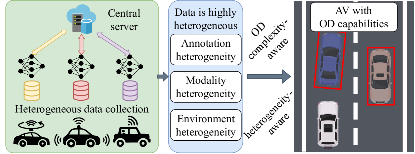
Our solutions. To tackle these challenges, we carefully re-engineer the classical two-stage OD model (Ren et al., 2015) to accommodate the multimodal data generated on AVs, and we exploit a major insight on the loss surface of OD under FL to guide the design of several learning mechanisms that handle the heterogeneity issue, as briefly illustrated in Figure 1. Since we notice that tolerance for data anomalies is crucial to efficiently navigate on the chaotic loss surface, we focus on robust designs to achieve such tolerance. Specifically, we design a cross-entropy-based loss function for training the neural model to handle unlabeled regions (of certain vehicles) that could be mistakenly regarded as the background during training. AutoFed also employs inter-modality autoencoders to perform data imputation of missing sensor modalities. The autoencoders learn from incomplete data modality and generate plausible values for the missing modality. Finally, AutoFed exploits a novel client selection mechanism to handle environment heterogeneity by eliminating diverged models. All in all, these three mechanisms together may largely avoid data abnormality and hence prevent the clients’ losses from falling into local minimums on the chaotic loss surface. Our key contributions can be summarized as follows:

• To the best of our knowledge, AutoFed is the first FL system specifically designed for multi-modal OD under heterogeneous AV settings.

• We design a novel cross entropy loss for training the neural model for OD, aiming to mitigate the annotation heterogeneity across clients.

• We design an inter-modality autoencoder to perform missing data modality imputation, thus alleviating the modality heterogeneity across the clients.

• We design a novel client selection mechanism for choosing mutually-enhancing clients, thus further eliminating the harmful effects induced by heterogeneity.

• We implement AutoFed prototype and evaluate AutoFed with extensive experiments. The promising results demonstrate that AutoFed can enable robust vehicle detection under AD scenarios.

Whereas most FL proposals consider only basic learning tasks (Konečnỳ et al., 2014; Li et al., 2020, 2021; Tu et al., 2021), AutoFed pioneers in FL-driven AV-OD far more sophisticated yet realistic than basic classification or regression. In the following, § 2 motivates the design of AutoFed by revealing the damaging effects of the heterogeneity. § 3 presents the system design of AutoFed. § 4 introduces the datasets, system implementation, and experiment setup, before reporting the evaluation results. Related works and technical limitations are discussed in § 5. Finally, § 6 concludes the paper with future directions.

2. Motivation

We first investigate the impact of annotation heterogeneity on the performance of a DNN model for vehicle detection. Then we show that the heterogeneous modality significantly degrades the performance of the federated model on OD. Finally, we confirm the necessity to tackle the model divergence potentially caused by heterogeneous factors (e.g., diversified environments and human inputs) in federated training.

2.1. Quantity Skew of Labeled Data

As an FL system, AutoFed relies on AV clients to provide labels (i.e., bounding boxes around vehicles) for two reasons: i) the server should not have access to local data due to privacy concerns; and ii) labeling data locally is more reasonable compared to performing the labeling offline on the server, because more visual cues can be leveraged for labeling locally on AVs, and we hence deem all such labels as reliable. However, relying on clients for data labeling can lead to skew in label quantity: some clients may be more motivated to provide annotations with adequate quality, while others may be so busy and/or less skillful that they miss a large proportion of the annotations. The situation may get worse during training, as the missing annotations on some AVs could be mistakenly marked as background by the OD network, thus backpropagating wrong gradients during local training. As a result, the small number of labels on some AVs may degrade the overall performance and cause training instability of the OD network.

(a) Average precision.

(b) Average recall.

Figure 2. Damaging effects of missing annotations.

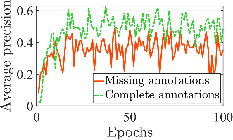
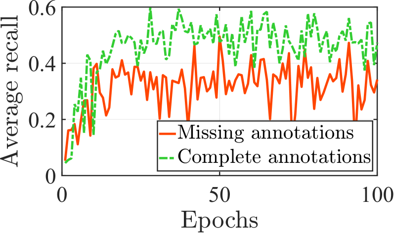
To demonstrate the damaging effects of missing labeling, we show the average precision and recall of a two-stage OD network for the task of vehicle detection in Figure 2. The network utilizes a VGG variant (Simonyan and Zisserman, 2014) as its backbone and was trained by standard backpropagation using an SGD optimizer on a dataset of 1,000 data samples with 50% data with missing annotations and 50% data with complete annotations in a standalone manner. After training, the network is tested on another 1,000-sample dataset. Clearly, the network under complete labeling outperforms that under missing labeling by around 20% in terms of both precision and recall. Moreover, it is evident that the performance of the DNN under missing labeling experiences a downward trend after the 20-th epoch, confirming the negative effects of the wrong gradient signals introduced by missing labeling.

2.2. Heterogeneous Modality across AVs

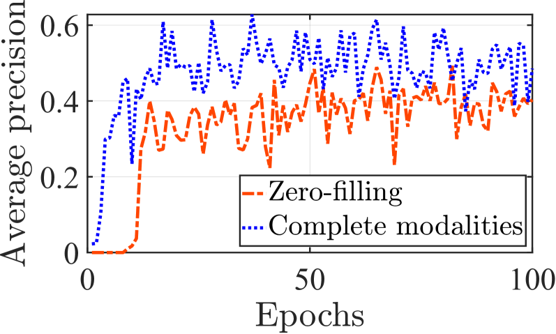
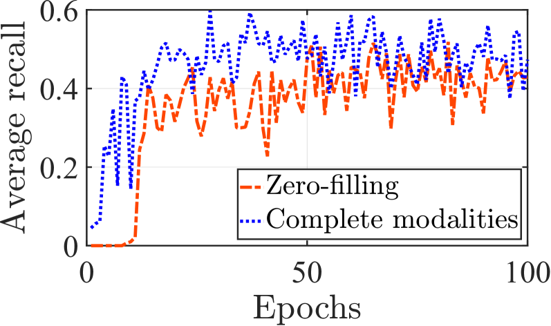
Most prior work on the fusion of multimodal sensing data assumes that all modalities are available for every training data point (Xu et al., 2018; Bijelic et al., 2020). This assumption may not be valid in reality, as the sensing modalities of different AVs are often heterogeneous for two reasons. On one hand, the AVs may be equipped with different types of sensors by their manufacturers. On the other hand, even for AVs from the same manufacturer, it is common that certain sensor experiences malfunctions, causing corresponding data modality to get lost. Such heterogeneous modalities pose significant challenges to DNN-based OD. Removing data entries with missing modalities or keeping only modalities shared among all clients can be a makeshift, but useful information conveyed in other modalities or clients can be discarded. Lacking access to global statistics also renders filling a missing modality with typical statistics (e.g., mean) impractical, leaving zero-filling (Van Buuren, 2018) as the only possibility. Therefore, we show the average precision and recall of an OD network in Figure 3; the model is trained in a standalone manner under complete modalities and missing modalities with zero-filling. In the training process, data with missing radar and lidar each accounting for 25% of a 1,000-sample dataset. The results demonstrate that the precision and recall of training the models with complete modalities outperform those with partial modalities by more than 20% and 10%, respectively, confirming that zero-filling does not fully overcome the challenge. To mitigate the missing modality, it is necessary to propose a new data imputation technique.

(a) Average precision.

(b) Average recall.

Figure 3. Damaging effects of missing modality.

2.3. Model Divergence

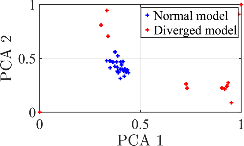
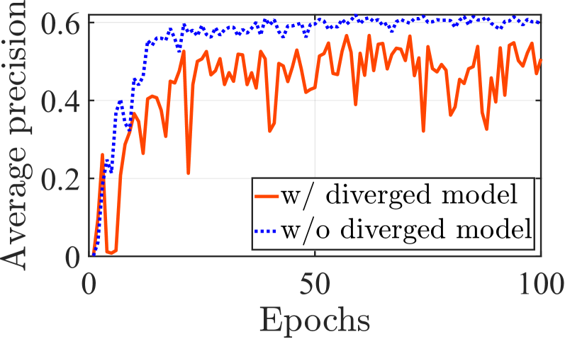
Besides the above label and modality heterogeneity across the clients, there exist other heterogeneities such as those introduced by environments (e.g., different weather and road conditions). Such heterogeneity makes the local models on AVs to be diverged and the optimization goal can even become contradictory. We demonstrate such model divergence in Figure 4a, where we involve 40 clients each holding a 1,000-sample dataset for training. These datasets have i) annotation level ranging from 10% to 100% (with 10% step size for every 4 clients), ii) 25% chance to hold data with missing radar or lidar modality, and iii) equal chance to have data recorded under clear, foggy, rainy, and snowy weather. After training, the network is tested on another 2,000-sample dataset. We apply PCA (principal component analysis) (Pearson, 1901) to the model weights at the 10-th epoch, and visualize the first two PCA components, one may readily observe that, while about half of local model weights form a cluster (colored in blue), there exist multiple outliers (colored in red). If we recklessly perform aggregation on these model weights, the performance of federated model will be significantly degraded by the outliers. We demonstrate the effects of diverged models in Figure 4b. The results show that aggregating the diverged models leads to a 10% drop in OD precision when compared with the aggregated model from homogeneous training data.

(a) PCA embedding.

(b) Average precision.

Figure 4. Damaging effects of diverging models.

3. System Design

Based on our discussions in § 2, we hereby present AutoFed comprising a two-level design: i) a multimodal OD network to fully exploit the information provided by multimodal sensors equipped on the AVs, and ii) an FL framework involving specifically designed loss, missing modality completion module, and client selection mechanism, aiming to achieve heterogeneity-aware federated multimodal OD on distributed AVs. In the following, we first define our problem concretely, and then we present the details of the multimodal OD network and FL framework.

3.1. Problem Statement and Overview

The ultimate goal of AutoFed is to make use of the crowdsensed data collected from multiple AVs (i.e., clients) to increase the data diversity, thus improving upon the performance of a standalone OD network deployed on a single client. Since the sensors on AVs can have multiple viewing perspectives, i.e., the lidar, radar, and camera have 3D, bird’s-eye view, and front view, respectively, there are no one-size-fits-all solutions. Therefore, we specifically choose to solve the vehicle detection problem (Petrovskaya and Thrun, 2009) (a special case of OD) from the bird’s-eye view using lidar and radar, thanks to (also confined by) the availability of dataset and vehicle annotations (Barnes et al., 2019). We avoid using camera in AutoFed for two reasons. First, the perception capability of lidar and camera largely overlap due to their similar spectrums. Second, the current settings and network architecture mostly are focused on the bird’s eye view of the vehicle’s surroundings, making the camera’s orthogonal front view largely incompatible. Note that our AutoFed framework is not limited to any specific OD tasks, because performing vehicle detection actually encompasses all critical elements in fulfilling other OD tasks.

Since AV scenarios are by default a distributed setting, FL is a good candidate for better utilizing the data diversity from geographically distributed clients. However, combining FL with OD may exacerbate OD’s chaotic loss surface emphasized in § 1, forcing naive aggregation algorithms to yield only comparable or even inferior performance compared to traditional standalone training (Liu et al., 2020; Jallepalli et al., 2021; Yu and Liu, 2019), especially under the challenges mentioned in § 2. Fortunately, our insight indicates that high tolerance to data anomalies can often allow effective training that leads to meaningful local minimums, by smoothly navigating on the chaotic loss surface; this motivates our following design considerations. Firstly, both data preprocessing and network architecture should be modularized and flexible enough to accommodate potentially abnormal multimodal inputs. Secondly, the network should be equipped with a mechanism to tolerate annotation anomalies of the input data. Thirdly, there should be a way to fill in missing modalities without making the data distributions abnormal. Finally, the aggregation mechanism must be sufficiently robust to withstand potentially diverging client models that could result in a non-optimal outcome after aggregation.

3.2. Multimodal Vehicle Detection

Before introducing the AutoFed framework, we first look at how to design a multimodal OD network under an FL setting. While the design method of a conventional two-stage OD network is well-established, how to integrate multimodal processing into the network remains an open issue. Furthermore, extending the multimodal OD network to the FL scenario put more stringent requirements on handling of the multimodal data. Intuitively speaking, different data modalities of such a network should i) conform to similar data formats, thus facilitating multimodal fusion, ii) collaborate by sharing information so as to enhance other modalities, and iii) be loosely coupled so as to support a more flexible FL pipeline that better deals with heterogeneous data and environment. In this section, we start with introducing the basics of the conventional OD network. Then we align lidar and radar data for improving data compatibility, in order to satisfy the requirement i). Finally, we present a novel feature-level fusion technique to satisfy the other two requirements with strong information sharing and loose coupling among the modalities.

3.2.1. Object Detection Basics

Figure 5. The upgraded OD pipeline of AutoFed’s multi-model vehicle detection network.

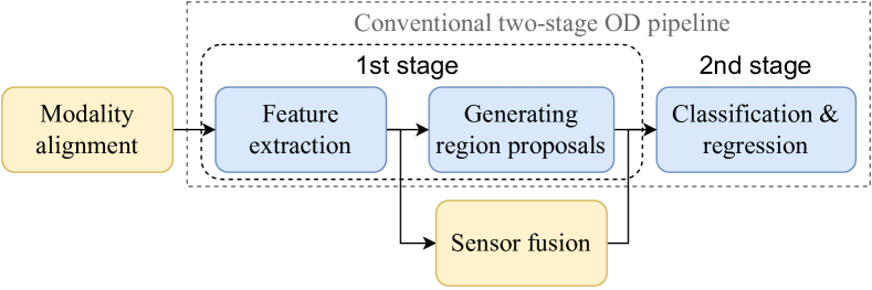
Conventional two-stage OD follows 3 major steps (Girshick, 2015; Ren et al., 2015), with 2 steps in the first stage as shown by the “blue” boxes in Figure 5. Generally, a feature map is first extracted using well-accepted feature extractors (e.g., VGGNet (Simonyan and Zisserman, 2014) or ResNet (He et al., 2016)), then region proposals are generated by the region proposal network (RPN). Specifically, taking the feature maps as input, RPN generates anchor boxes with pre-defined fixed scales and aspect ratios. The built-in classifier of RPN differentiates whether each anchor box is foreground or background. The outcome allows RPN to generate the region proposals; it leverages a built-in regressor to fit the anchor boxes to their corresponding objects by adjusting their offsets. With the above completing Step-1, Step-2 involves the region proposals being filtered by non-maximum suppression (NMS): the proposals with the highest confidence are selected and excessive proposals overlapping with higher-confidence proposals above a given threshold are removed. The loss of RPN is $L^{\mathrm{RPN}}=L_{\mathrm{cls}}^{\mathrm{RPN}}+L_{\mathrm{loc}}^{\mathrm{RPN}}$, where $L_{\mathrm{cls}}^{\mathrm{RPN}}$ is a binary cross entropy (BCE) loss measuring the “objectness” of the classification (i.e., how good the RPN is at labelling the anchor boxes as foreground or background), and $L_{\mathrm{loc}}^{\mathrm{RPN}}$ is an $L^{1}$ loss quantifying the localization performance of the predicted regions generated by the RPN.

The second stage (also Step-3) performs a fine-tuning to jointly optimizes a classifier and bounding-box regressors. After cropping out the feature map and RoI pooling (Ren et al., 2015) of the interested region according to the generated proposals, it further uses a classifier to detect whether the generated bounding box contains a specific class of object. It also fine-tunes the bounding boxes using a class-specific regressor. Essentially, this stage introduces three losses, i.e., a BCE classification loss $L_{\mathrm{cls}}$ measuring the network performance in labeling a predicted box with an object, an $L^{1}$ box regression loss $L_{\mathrm{reg}}$ quantifying how the predicted location deviates from the true location, and a BCE direction loss $L_{\mathrm{dir}}$ specifying whether the vehicle is pointing upward or downward to remove ambiguity, thus confining the possible angles of the rotated bounding box to be in the range of $[0^{\circ},180^{\circ}]$. In summary, the overall loss function for the OD network can be written as:

(1) $$L_{\mathrm{total}}=L^{\mathrm{RPN}}+L_{\mathrm{cls}}+L_{\mathrm{reg}}+L_{\mathrm{dir}}$$

Figure 6. AutoFed architecture: Federated multimodal learning with heterogeneity-awareness.

3.2.2. Modality Alignment

The heterogeneous data generated by multiple modalities poses a challenge to conventional OD network. Specifically, the input 3-D lidar point clouds and mechanically scanned 2-D radar heatmap are incompatible and cannot be readily fused or imputed (as will be explained in § 3.3.2) on both the original data space and the feature space. To reconcile the incompatibility, we first voxelize the 3-D point cloud obtained by lidar (Yang et al., 2018). Since we are interested in performing vehicle detection from the bird’s-eye view, the horizontal 2-D slices of the resulting lidar data can be deemed as an image with 36 channels, i.e., 35 channels depicting the point occupancy in the space and 1 channel indicating the overall intensity of the lidar signals obtained on the horizontal plane. Similarly, the radar signal can be deemed as an image with a single channel since it has no 3-D information. After converting the data into “multi-channel” images, they are further registered by considering the extrinsics and resolutions of the sensors, as well as vehicle kinematics. Finally, two independent yet identical feature extractors (those of the OD network as shown on the left side of Figure 5) are used to process lidar image $\mathbf{x}_{l}\in\mathcal{L}$ and radar image $\mathbf{x}_{r}\in\mathcal{R}$, where $\mathcal{L}$ and $\mathcal{R}$ are the datasets containing lidar and radar images, respectively. While the same architecture of these feature extractors guarantees that the modality alignment is preserved on the feature space, they differ in the number of input channels to cater the respective needs of lidar and radar data.

3.2.3. Feature-Level Sensor Fusion

Two approaches exist for fusing multimodal data, i.e., data-level and feature-level fusion. AutoFed opts for feature-level fusion thanks to its better flexibility and low coupling offered by fusion at a later stage in the network. Specifically, to extend the OD network in § 3.2.1 to a multimodal setting, we further add parallel feature extractors for other modalities. Suppose the feature extractors output lidar feature map $\mathbf{z}_{l}$ and radar feature map $\mathbf{z}_{r}$, one naive method to perform feature-level fusion would be to concatenate $\mathbf{z}_{l}$ and $\mathbf{z}_{r}$, and feed the concatenated features to Step-2 of the OD network. However, this straightforward method fails to exploit the inter-modality relationship. A more relevant approach for exploiting the relationship is to apply the cross-attention mechanism (Wei et al., 2020). It generates an attention mask, in which information from a different modality is harnessed to enhance the latent features of the interested modality (e.g., an attention mask derived from lidar is used to enhance radar features, and vice versa). Different from the existing self-attention mechanism (Vaswani et al., 2017), our cross-attention mechanism focuses on modeling the cross-correlation among different modalities, and it adaptively learns the spatial correspondence to derive better alignment of important details from different modalities.

Essentially, our cross-attention mechanism can be described as transforming the latent representation $\mathbf{z}$ to a query $\mathbf{q}$ and a set of key-value pair $\mathbf{k}$ and $\mathbf{v}$, and then mapping them to an output. The query, keys, and values are all linearly transformed versions of the input $\mathbf{z}_{s}\!:s\in\{\text{lidar},\text{radar}\}$:

(2) $$\mathbf{q}_{s}=\mathbf{W}_{q}\mathbf{z}_{\bar{s}}+\mathbf{b}_{q},~{}~{}~{}\mathbf{k}_{s}=\mathbf{W}_{k}\mathbf{z}_{\bar{s}}+\mathbf{b}_{k},~{}~{}~{}\mathbf{v}_{s}=\mathbf{W}_{v}\mathbf{z}_{s}+\mathbf{b}_{v},$$

where $\bar{s}$ is the complementary sensing modality of $s$ (e.g., if $s$ is radar, then $\bar{s}$ is lidar, and vice versa), $\mathbf{W}_{q}$, $\mathbf{W}_{k}$, $\mathbf{W}_{v}$ and $\mathbf{b}_{q}$, $\mathbf{b}_{k}$, $\mathbf{b}_{v}$ are trainable matrices and vectors that help transforming the input to its corresponding query $\mathbf{q}_{s}$, key $\mathbf{k}_{s}$, and value $\mathbf{v}_{s}$, whose dimensions are denoted by $d_{q}$, $d_{k}$, $d_{v}$, respectively. The output context $\mathbf{z^{\prime}}_{s}$ is obtained as a weighted sum of the values in $\mathbf{v}_{s}$, where the weight of each value is a normalized product of the query $\mathbf{q}_{s}$ and its corresponding key $\mathbf{k}_{s}$: $\mathbf{z^{\prime}}_{s}=\operatorname{softmax}\left(\frac{1}{\sqrt{d_{k}}}\mathbf{q}_{s}\mathbf{k}_{s}^{T}\right)\mathbf{v}_{s}.$

3.3. AutoFed Framework

We intend to design an FL framework that extends our multimodal vehicle detection network in § 3.2 to a training scenario where the data are collected by geographically distributed AVs. As illustrated in Figure 6, AutoFed improves the multimodal vehicle detection network in three aspects: i) modifying the loss of RPN to deal with client annotation heterogeneity, ii) employing an autoencoder to perform data imputation of missing sensing modalities, and iii) applying a client selection strategy based on $k$-d tree (Bentley, 1975) to overcome the diverged models brought by the environment and aforementioned heterogeneity.

3.3.1. Modified Loss Function for Tolerating Annotation Anomalies

As stated in § 2.1, the heterogeneity of labeled data may send wrong gradient signals during AutoFed training, since the bounding boxes that should be classified as foreground otherwise can be wrongly labeled as background when their correct annotations are missing. The motivation for our modified loss is that, despite the lack of correct annotations, the AutoFed model can identify vehicles wrongly labeled as backgrounds according to its own well-established classifier, thus avoiding sending erroneous gradient signals during backpropagation and better guiding the convergence on the OD loss surface mentioned in § 3.1. Specifically, if the feature map of an anchor region is found to be similar to a vehicle, the classifier naturally assigns a high probability $p$ of predicting it as a vehicle. This comes under a reasonable assumption that, since the global model is trained sufficiently with on average high-quality annotations, it can be more trustworthy than the annotations from a few incompetent clients. Recall the BCE loss of RPN in § 3.2.1 as: $L_{\mathrm{cls}}^{\mathrm{RPN}}=-p^{*}\log\left(p\right)-\left(1-p^{*}\right)\log\left(1-p\right)$, where $p^{*}$ is the training label taking on values of 0 or 1, respectively indicating the bounded region being background or vehicle. Consequently, the modified cross-entropy (MCE) loss becomes:

(3) $$\left\{\begin{matrix}0,&p>p_{\mathrm{th}}~{}\text{and}~{}p^{*}=0,\\ -p^{*}\log p-(1-p^{*})\log(1-p),&\text{otherwise},\end{matrix}\right.$$

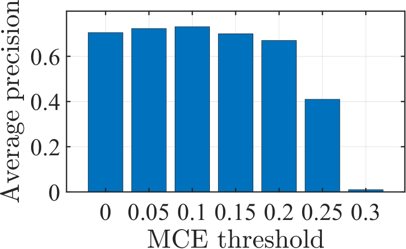
where $p_{\mathrm{th}}$ is a threshold value after which we believe that the classifier is more trustworthy than the annotations. The value of $p_{\mathrm{th}}$ is determined by hyperparameter search in § 4.7.1.

(a) Average precision.

(b) Average recall.

Figure 7. Comparison between CE and MCE loss.

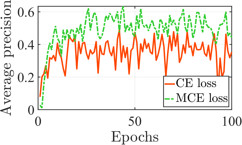
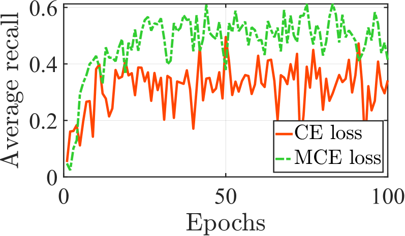
To demonstrate the efficacy of the MCE loss, we train a multimodal vehicle detection network using the settings in § 2.1. The training results of regular CE loss and our MCE are shown in Figure 7; they evidently confirm the superiority of MCE loss, though the average precision and average recall of both CE and BCE losses fluctuate around their means after sufficient training (approximately 15 epochs). First of all, The average precision of vehicle detection is respectively 0.57 and 0.4 when CE and MCE loss are used. Similarly, there is a gap greater than 0.1 in the average recalls when the two losses are used. Moreover, it is clear that, though training with CE loss achieves higher precision and recall in the few initial epochs, it is quickly overtaken by the MCE loss, which keeps an upward trend and converges faster. Last but not least, one may also observe that there is a slight downward trend of performance when the CE loss is used after the 15-th epochs. The performance gaps and different performance trends clearly demonstrate that our MCE loss can make full use of vehicle annotations while avoiding backpropagating erroneous gradients caused by missing annotations.

3.3.2. Modality Imputation with Autoencoder for Tolerating Modality Anomalies

We have shown in § 2.2 that conventional data imputation methods (e.g., filling the missing modalities with 0’s) incurs information loss, and may even introduce biases into the network. To leverage the valuable information in the heterogeneous sensing modalities, we propose to fill in the missing data by leveraging the relations among different modalities. Since different modalities are aligned and loosely coupled (as explained § 3.2.2 and § 3.2.3), we employ a convolutional autoencoder with residual connections (which connects a layer to further layers by skipping some layers in between, thus facilitating information flow) to directly perform modality imputation. The encoder of the autoencoder consists of 4 convolutional layers, and correspondingly, the decoder of the autoencoder consists of 4 transposed convolutional layers. Consequently, the lightweight architecture of our autoencoder only incurs negligible overhead representing an increase of only 4.38% (3.129 ​GFLOPS vs. 2.988 ​GFLOPS) from the AutoFed variant without autoencoder. It should be noted that the autoencoder is pre-trained and does not participate in the training process of AutoFed. During the pretraining stage, the autoencoder aims to learn a latent representation, and reconstruct the missing modality. For example, when the radar modality $\mathcal{R}$ is missing, the autoencoder encodes the lidar modality $\mathcal{L}$ and translates the latent information therein to fill in the missing radar modality.

(a) Average precision.

(b) Average recall.

Figure 8. Modality imputation with an autoencoder.

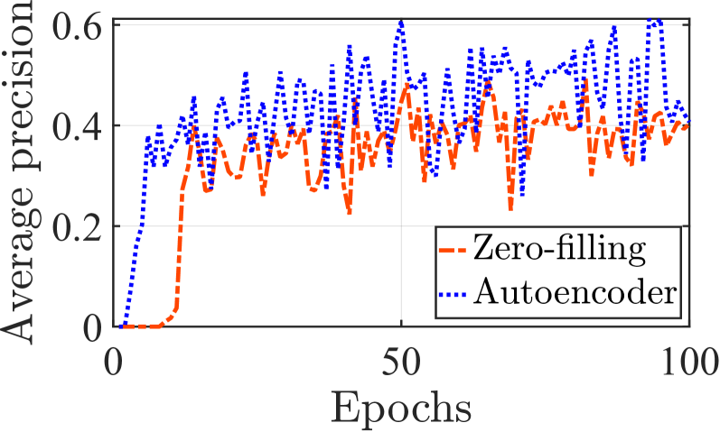
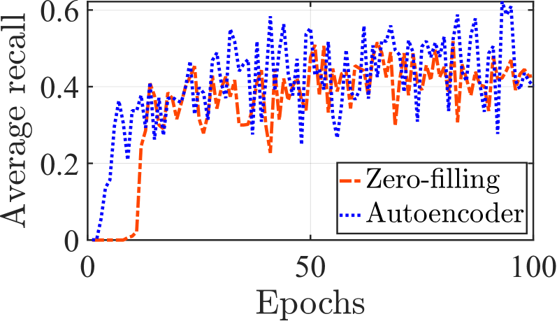
To show the efficacy of the above method, we train the multimodal vehicle detection network following the settings in § 2.2, and compare the average precision and recall of autoencoder imputation with zero-filling in Figure 8a and 8b, respectively. One may readily observe that zero-filling only achieves an average precision of approximately 0.4, lower than an average precision of about 0.5 achieved by our autoencoder imputation. Similarly, autoencoder imputation also surpasses zero-filling in terms of average recall by a discernible margin. Figure 8 also indicates that autoencoder imputation only takes about 5 epochs to converge, much faster than the convergence speeds (i.e., 10 and 15 epochs) by zero-filling. The higher average precision and recall, as well as the faster convergence training speed have clearly demonstrated that our designed autoencoder makes full use of the heterogeneous data by taking into account the correlations among different modalities.

3.3.3. Client Selection for Tolerating Model Weight Anomalies

Environment heterogeneities, including different weather and road conditions (as indicated in § 2.3), as well as other human-induced heterogeneities (e.g., inaccurate annotations), are not easily solvable using the techniques described in Sections 3.3.1 and 3.3.2, yet they can cause serious model divergence among the clients. Training with diverging clients holding extremely biased datasets may contradict models from other clients, thus increasing the overall losses. To make things worse, the chaotic loss surface mentioned in § 1 and § 3.1 can disorient the gradient descent algorithm used for training the OD model, and further diverge the model weights. These observations urge us to devise a novel client selection strategy immune to divergence, rather than blindly using FedAvg to aggregate model weights from all clients equally. By selectively removing outlier clients, the client selection strategy should help the loss navigating on the surface more efficiently.

Suppose there are $N$ clients $\{C_{1},\cdots,C_{n},\cdots,C_{N}\}$ in total, which forms a set $S$. To mitigate the issue of diverged models, we would like to dynamically select a subset $S^{\prime}=\{C_{1},\cdots,C_{m},\cdots,C_{M}\}$ of $M$ clients ($M<N$) after each FL communication round to minimize the sum of inter-client distances of model weights. To achieve this, we propose that, after receiving the local models from the clients, the central server constructs a $k$-d tree using the received model weights. The $k$-d tree is a bisecting structure where each branch point is the median in some dimension, and this bisecting structure helps improve the efficiency of finding the nearest client (local) models with minimum distances. Subsequently, the central server traverses every client in the set $S$, and queries its $M-1$ nearest neighbors efficiently using the $k$-d tree data structure. The client with the minimum distance sum to its $M-1$ neighbors, together with its $M-1$ neighbors, form the subset of selected clients $S^{\prime}$. Since the time complexity of one query is $O(\log{N})$, traversing the whole set $S$ demands a complexity of $O(N\log{N})$, which saves up a lot of time when compared with $O(N^{2})$ complexity of brute-force search, especially when there are many clients involved. At last, the central server aggregates the model weights from the selected clients in subset $S^{\prime}$, and distributes the updated global model to all clients in $S$ for training in the next communication round.

(a) PCA embedding.

(b) Average precision.

Figure 9. Client selection mitigates diverged models.

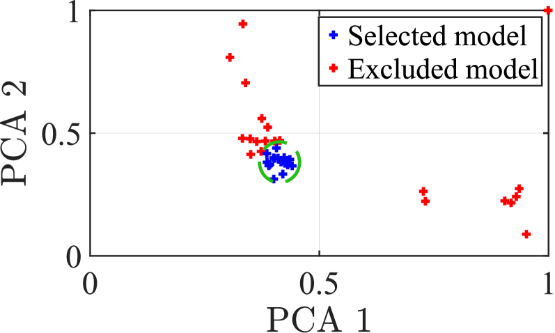
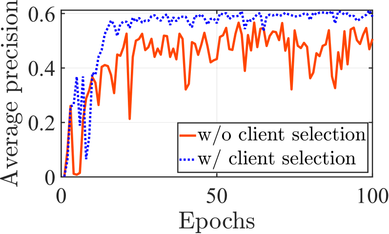
To illustrate the effect of our client selection strategy, we train the multi-modal vehicle detection network following the settings in § 2.3. After each communication round, we let the central server selects 40% of the clients (i.e., $M=0.4N$) to form a subset of clients with minimum inter-client local model weight distance, as demonstrated in Figure 9a. The average vehicle detection precision is shown in Figure 9b. One may readily observe that the precision of vehicle detection reaches up to 0.6 when client selection is enabled, and it fluctuates around 0.5 when model weights from all clients are aggregated using the FedAvg algorithm. Moreover, Figure 9 also demonstrates that client selection makes the training converge faster with less than 20 epochs, while the training without client selection barely starts to converge till the 25-th epoch. These phenomena indicate that client selection helps better utilize data from beneficial clients. Upon further inspection, we find that after convergence, the fluctuation of the precision curve with client selection is much smaller than that without client selection, which indicates that the mechanism indeed selects mutually-enhancing clients while excluding erroneous gradient signals from outliers. Additionally, it can be observed that the average precision with client selection becomes stable after only 70 epochs. This confirms that the model has effectively learned from all clients (including the corner cases), so additional training will not yield any further improvement in performance.

1

Require : $N$ is the total number of clients, $c$ is the percentage of clients to choose.

Data: $\{(\mathcal{L}_{1},\mathcal{R}_{1}),\cdots,(\mathcal{L}_{n},\mathcal{R}_{n}),\cdots,(\mathcal{L}_{N},\mathcal{R}_{N})\}$ where $(\mathcal{L}_{n},\mathcal{R}_{n})$ is the local collected lidar and radar data on the $n$-th AV.

2

3Server Executes:

4       initialize the global model $w^{g}_{0}$ at $t=0$;

5       $S\leftarrow\{C_{1},\cdots,C_{N}\}$;

6       for communication round $t$ do

7             for $C_{n}\in S$ in parallel  do

8                   $w_{t+1,n}\leftarrow\textnormal{{Client Update}}(n)$;

9                   $W_{t}\leftarrow W_{t}\cup w_{t+1,n}$;

10                  

11            $M\leftarrow c\times N$;

12             $W_{t}^{\prime}\leftarrow\textnormal{{Client Selection}}(W_{t},M)$;

13             $w^{g}_{t+1}\leftarrow\textnormal{{Model Aggregate}}(W_{t}^{\prime})$

14Client Update($n$):

15       $w_{n}\leftarrow w_{t}^{g}$ ($w_{t}^{g}$ is downloaded global model) ;

16       if $\mathcal{R}_{n}=\varnothing$ then

17             $\mathcal{R}_{n}\leftarrow$ Radar Imputation ($\mathcal{L}_{n}$);

18            

19       else if $\mathcal{L}_{n}=\varnothing$ then

20             $\mathcal{L}_{n}\leftarrow$ Lidar Imputation ($\mathcal{R}_{n}$);

21            

22       for each local epoch $e$ do

23             for each batch $b$ do

24                   $w_{n}\leftarrow$ SGD($w_{n},b$) ;

25                  

26      return $w_{n}$;

27      

28Client Selection($W_{t}$, M):

29       $T_{t}\leftarrow\textnormal{{Construct k-d Tree}}(W_{t})$;

30       for $C_{i}\in S$ do

31             $S_{i}\leftarrow\textnormal{{Query k-d Tree}}(T_{t},C_{i},M)$;

32             $d_{i}\leftarrow\Sigma_{m=1}^{M}\textnormal{{Dist}}(C_{i},C_{m})$ for $C_{m}\in S_{i}$;

33            

34      $I_{min}=\operatorname*{arg\,min}_{i}(d_{i})$;

35       for $C_{m}\in S_{I_{min}}$ in parallel  do

36             $W_{t,I_{min}}^{\prime}\leftarrow W_{t,I_{min}}^{\prime}\cup w_{t,m}$;

37            

38      return $W_{t,I_{min}}^{\prime}$;

39      

Algorithm 1 AutoFed training.

3.3.4. Putting It All Together

We carefully summarize the training strategy of the AutoFed framework in Algorithm 1. In the algorithm, Client Update is the local training process for each client, Radar Imputation and Lidar Imputation are the imputation function introduced in § 3.3.2, SGD is the standard stochastic gradient descent algorithm with our MCE loss, Client Selection has been introduced in § 3.3.3, which includes Construct k-d tree and Query k-d Tree as the respective processes of constructing and querying $k$-d tree, as explained in § 3.3.3, and Model Aggregate as the standard process of averaging the selected local models. By putting together AutoFed’s modules, we create a cohesive ensemble to substantially enhance the tolerance to data anomalies. Although some techniques can be relevant even to a single model context, they work together in the FL setting to help AutoFed navigate on the chaotic loss surface in a more robust and efficient manner.

4. Performance Evaluation

To evaluate the performance of AutoFed, we apply AutoFed to build a vehicle detection application using the benchmark dataset (Barnes et al., 2019). In particular, we evaluate the performance of AutoFed from four aspects: i) comparisons with five baseline methods to demonstrate the superiority of AutoFed; ii) cross-domain tests to show that AutoFed is robust against real-life scenarios with heterogeneous data; iii) ablation study to show the necessity of key parameter designs, and iv) investigating the impact of FL-related hyper-parameter on the model performance.

4.1. Dataset

We mainly use the Oxford Radar RobotCar dataset (Barnes et al., 2019) in our experiment. The dataset is collected by a vehicle driving around Oxford, and it includes both lidar and radar data. The lidar data is obtained by merging the point clouds collected by two Velodyne HDL-32E (Velodyne Lidar, Inc., 2022) lidars mounted on the left and right of the vehicle’s top. Each lidar sensor provides a range of 100 ​m, a range resolution of 2 ​cm, a horizontal field of view (FoV) of 360^∘, and a vertical FoV of 41.3^∘. The radar data is collected by a millimeter-wave Frequency-Modulated Continuous-Wave (FMCW) NavTech CTS350-X radar (Navtech Radar, 2022) mounted between the two lidar sensors and at the center of the vehicle aligned to the vehicle axes. The radar achieves 2-D horizontal scan by rotation, operating with a center frequency of 76.5 ​GHz, a bandwidth of 1.5 ​GHz, a sampling rate of 4 ​Hz (hence a range resolution of 4.38 ​cm), a rotational angle resolution of 0.9^∘, a beamwidth of 1.8^∘, and a range up to 163 ​m; it complements lidar by providing robustness to weather conditions that may cause trouble to lidar. We further convert the data residing in the polar coordinates to Cartesian coordinates and then calibrate radar and lidar extrinsic parameters (i.e., translation and rotation with respect to the world) by performing pose optimization to minimize the differences between lidar and radar observations. Since there is no original ground truths for vehicle detections, we create rotated boxes by inspecting the point cloud data using Scalabel (Scalabel, 2022), which is a scalable open-source web annotation tool for various types of annotations on both images and videos.

We also involve another dataset nuScenes (Caesar et al., 2020) in our experiment to demonstrate AutoFed’s generalizability across datasets. The dataset contains 1 lidar and 5 radars: the lidar has 360^∘ horizontal FoV, 40^∘ vertical FoV, and 2 ​cm range resolution, while the 5 radars have 77 ​GHz center frequency and 0.1 ​km/h velocity accuracy. Unlike the radars in the Oxford dataset that perform fine-grained mechanical scans, the radars in the nuScenes dataset are fixed in positions and do not have scan capability. As a result, they only generate low-quality pointclouds. Since AutoFed cannot demonstrate its full potential with the inferior radar modality, we limit the evaluation on the nuScenes dataset to only § 4.4. For both datasets, we take out a total of 50,000 samples, and use 80% and 20% of the total data to create training and test datasets, respectively.

4.2. System Implementation

We implemented the vehicle detection application using AutoFed on multiple NVIDIA Jetson TX2 (NVIDIA, 2022) devices. The central server is equipped with an Intel Xeon Gold 6226 CPU (Intel Corporation, 2022) and 128 ​GB RAM. For both AutoFed and the baselines, we implement an FL protocol that allows 20 participating clients to randomly take 2,000 non-overlapping samples from the 40,000-sample training set. Each participating client performs 5 local training epochs for each communication round. As for the software, Python 3.7 and PyTorch 1.9.1 (Paszke et al., 2019) are used for implementing the application. Our vehicle detection model is built upon Detectron2 (Wu, Yuxin and Kirillov, Alexander and Massa, Francisco and Lo, Wan-Yen and Girshick, Ross, 2022), which is a Python library that provides state-of-the-art OD models. In particular, the settings for the multimodal vehicle detection model are as follows:

• The autoencoder is trained with 20,000 samples from the Oxford dataset, distinct (in terms of traffic, weather, and locations) from those used for training the rest of AutoFed.

• The angles of the rotated anchors used by the RPN are set to -90^∘, -45^∘, 0^∘, and 45^∘.

• Both lidar and radar feature extractors are composed of four consecutive convolutional layers with a kernel size of 3 and padding of 1.

• The aspect ratio of the anchors is set to 2.5 to conform to the length-width ratio of regular vehicles (Toyota Motor Sales, U.S.A., Inc., 2022).

• The IoU threshold (defined later) of NMS for removing excessive proposals during testing is set to 0.2.

In the local training process, we employ the SGD optimizer by setting the initial learning rate as 0.01 and the decay factor as 0.01.

(a) AP@IoU=0.5.

(b) AP@IoU=0.65.

(c) AP@IoU=0.8.

(d) AP@IoU=0.5:0.9.

(e) AR, maxDets = 1.

(f) AR, maxDets = 10.

(g) AR, maxDets = 100.

(h) Convergence time.

Figure 10. Comparing AutoFed with several baseline methods, in terms of FL convergence and communication overhead.

4.3. Experiment Setup

Baselines

To comprehensively evaluate the performance of AutoFed, we compare AutoFed against five baselines:

• Standalone trains a vehicle detection model using heterogeneous data (e.g., heterogeneous annotations, sensing modalities, and environments) locally without collaborations among clients.

• Standalone+ trains a vehicle detection model locally using the same setting as Standalone, but the data are sampled in a homogeneous way.

• FedAvg is the first and perhaps the most widely adopted FL method (McMahan et al., 2017). During training, all clients communicate updated local parameters to the central server and download the aggregated (i.e., averaged) global model for local training in the next round.

• FedCor is a correlation-based client selection strategy for heterogeneous FL (Tang et al., 2022). It formulates the goal of accelerating FL convergence as an optimization problems that maximizes the posterior expectation of loss decrease utilizing the Gaussian process.

• FedProx adds a proximal term to the loss function of local training to reduce the distance between the local model and the global model (Li et al., 2020), hence addressing both system and statistical heterogeneity.

In addition, we adopt the same multimodal vehicle detection model configuration for each baseline method as AutoFed. We also apply the same training settings and data configurations as AutoFed to the baseline methods, the results are reported after the same number of communication rounds. It should be noted that we use Standalone and Standalone+ as baselines to provide context for how better FL methods perform: it confirms that they do improve upon standalone training, because each client only has limited data in reality.

Evaluation Metrics.

Before introducing the evaluation metrics, we first define an important concept called IoU (intersection over union), which evaluates the overlap between two bounding boxes. Suppose the ground truth and predicted bounding boxes are $B_{gt}$ and $B_{p}$, respectively, then IoU is given by the overlapping area between the predicted bounding box and the ground truth bounding box divided by the area of union between them:

(4) $$\mathrm{IoU}=\frac{\mathrm{Area}(B_{p}\cap B_{gt})}{\mathrm{Area}(B_{p}\cup B_{gt})}$$

We define $\mathit{TP}$ as the number of correct detections (i.e., detections with an IoU greater than the predefined threshold), $\mathit{FP}$ as wrong detections (i.e., detections with an IoU smaller than the threshold), and $\mathit{FN}$ as the number of ground truths that are not identified. Based on these definitions, we define precision and recall as:

(5) $$\mathrm{Precision}=\frac{\mathit{TP}}{\mathit{TP}+\mathit{FP}},\quad\mathrm{Recall}=\frac{\mathit{TP}}{\mathit{TP}+\mathit{FN}}.$$

Since there is often a tradeoff between precision and recall, we also define an average precision (AP) value across all precision values from 0 to 1, thus summarizing the precision-recall curve. Moreover, we calculate the average recall (AR) value at IoU thresholds from 0.5 to 1, thus summarizing the distribution of recall values across a range of IoU thresholds (Lin et al., 2014). AP and AR are our key evaluation metrics hereafter.

4.4. Superiority of AutoFed

(a) Ground truth.

(b) AutoFed.

(c) Standalone.

(d) Standalone+.

(e) FedAvg.

(f) FedCor.

(g) FedProx.

Figure 11. Example detection results of AutoFed and other baseline methods.

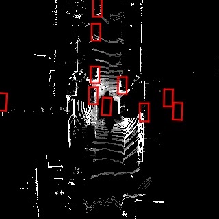
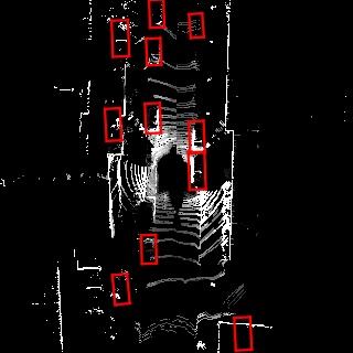
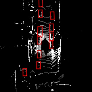
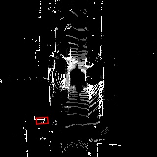
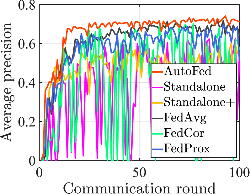
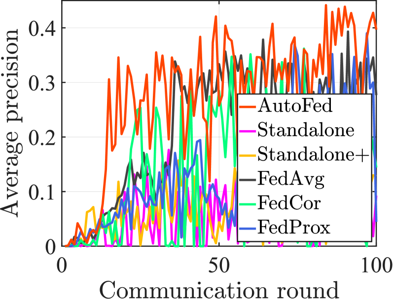
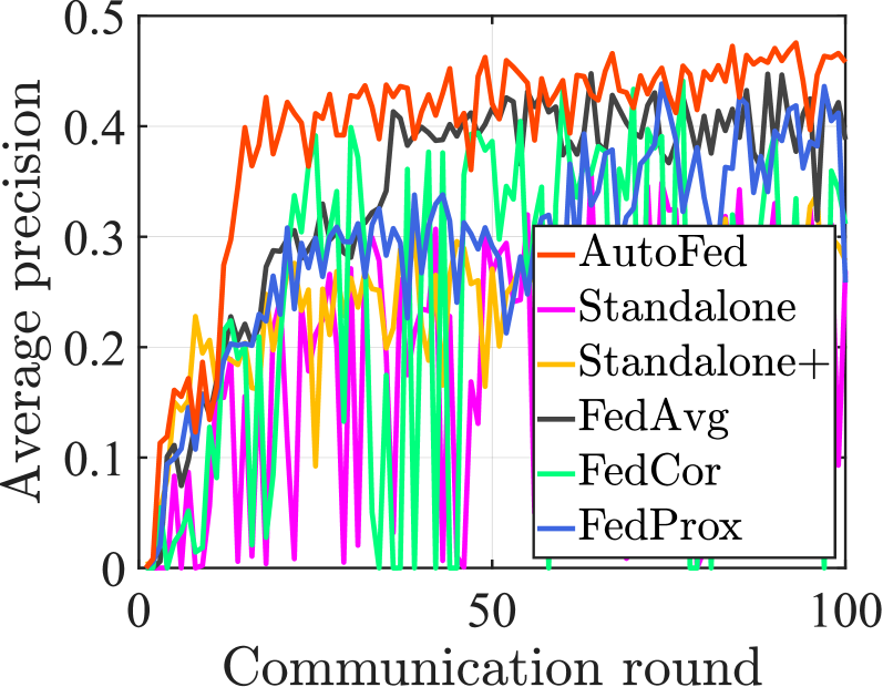
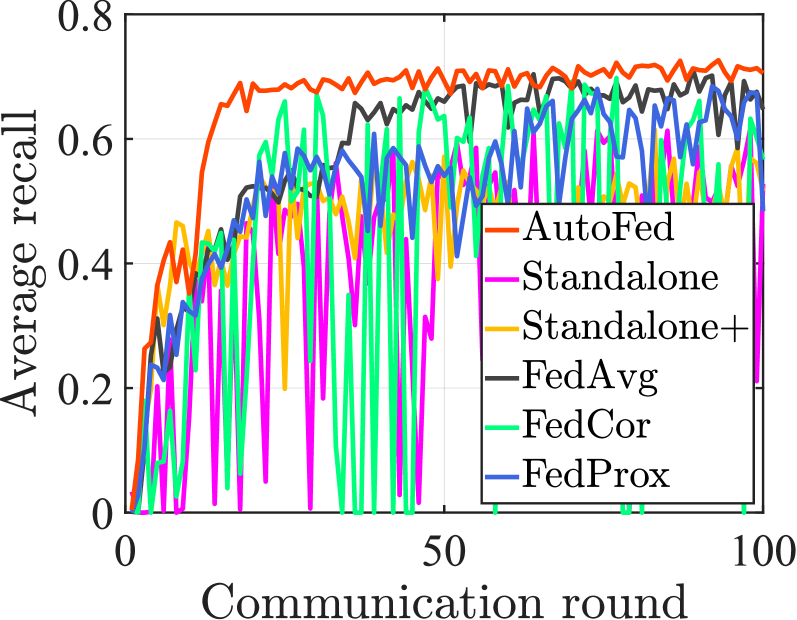
We compare AutoFed with the baselines in terms of the evaluation metrics defined in § 4.3. Specifically, we report AP when the IoU is 0.5, 0.65, and 0.8, respectively, and the mean AP when the IoU ranges from 0.5 to 0.9. As for AR, we focus on the cases when the number of maximum detections is 1, 10, and 100, respectively. We report the evaluation results in Figure 10. Figure 10a shows that, when the IoU is set as 0.5, the AP of AutoFed is 0.71 while the number of FedAvg and FedProx are 0.68 and 0.58, respectively. Moreover, the APs of Standalone, Standalone+, and FedCor oscillate dramatically and barely converge. Similarly, as shown in Figures 10b, 10c, and 10d, the performance of AutoFed significantly outperforms the baselines. It might be curious that the AP curve of AutoFed in Figure 10c appears to be fluctuating, but this can be readily attributed to the fact that setting IoU as 0.8 is a stringent criterion for the vehicle detection task and causes the performance to become unstable.

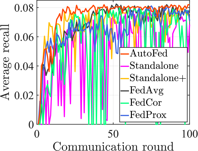
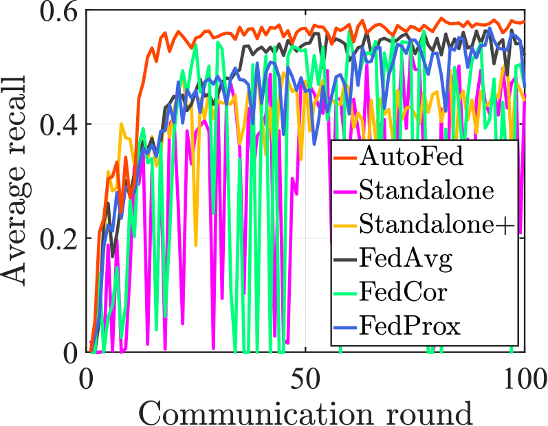
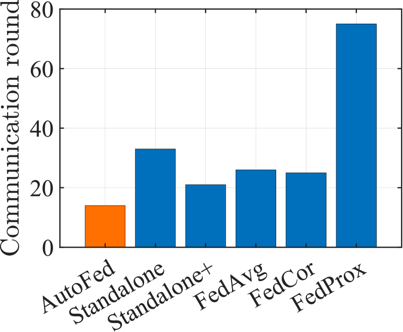
With regard to AR shown by Figures  10e, 10f, and 10g, AutoFed exhibits significantly better performance compared with the baselines, in terms of both AP and AR. Moreover, we also find that, when compared with the baselines, AutoFed reaches the maximum AP and AR with less number of communication rounds, as also confirmed by the results presented in Figure 10. Specifically, while AutoFed converges in 10 communication rounds, all baseline methods converge after 20 communication rounds. Furthermore, the AP and AR curves of AutoFed rarely fluctuate, and the training of AutoFed is much more stable than the baselines, indicating that the multimodal network trained by AutoFed is much more robust.

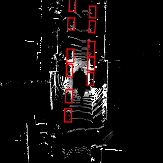
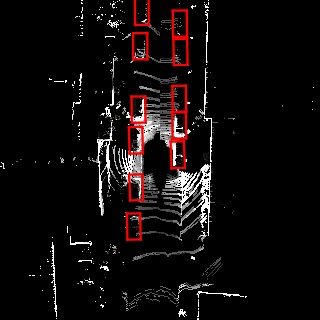
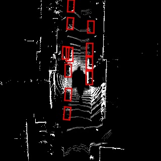
We also showcase some examples of vehicle detection in Figure 11. In the examples, we use the 2-D lidar intensity map as background for reference, and draw the ground truth and predicted bounding boxes upon it. Figure 11b shows that AutoFed generates high-precision vehicle detection results very close to the ground truth in Figure 11a. In contrast, the Standalone, Standalone+, and FedAvg methods make incorrect predictions outside the road, FedCor’s misses most of the vehicles, and FedProx misses some vehicles and generates inaccurate bounding boxes overlapped with each other. The results evidently confirm that AutoFed outperforms the baselines with more accurate predictions.

Furthermore, we compare the communication cost of AutoFed training (the same as other FL baselines) with centralized training, i.e., all the clients transfer the collected data to a central server for training the model. The results show that, while centralized training transfers 660000 ​KB of sensor data during each communication round per client, AutoFed only transfers 62246 ​KB of model weights. In other words, AutoFed reduces up to more than 10$\times$ communication cost per client than the centralized training, firmly validating its communication-efficient design.

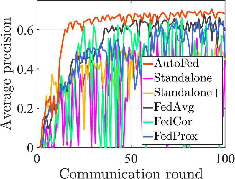
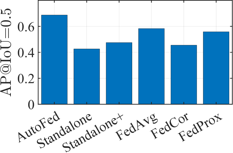
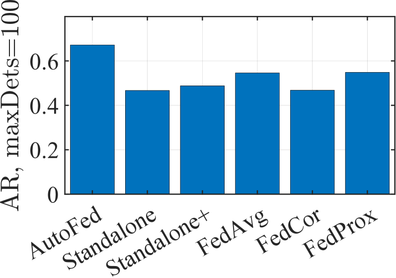
We finally compare the performance of AutoFed with the baselines on the nuScenes dataset (Caesar et al., 2020) to demonstrate its generalizability across different datasets. We train AutoFed for 100 communication rounds on the dataset. As shown in Figure 12, AutoFed outperforms all of the baselines on the nuScenes dataset by a large margin, firmly demonstrating that the evaluation results can be generalized to other datasets as well. It is worth noting that the overall AP and AR results of AutoFed on this dataset (0.687 and 0.672) are slightly lower than those shown in Figures 10a and 10g on the Oxford Radar RobotCar dataset, which can be attributed to a variety of factors, such as the complexity of the scenes and objects, sensor mounting positions, and most importantly, the sparsity and lower quality of the radar point cloud provided by the nuScenes dataset.

(a) Average precision.

(b) Average recall.

Figure 12. Evaluation on the nuScenes dataset.

4.5. Cross-domain Robustness

We evaluate the robustness of AutoFedin cross-domain settings by investigating how the trained model performs in varied sensing modalities and different weather conditions. Since the AVs’ routes in the experiment encompass different roads and areas, the results in § 4.4 have already proven the cross-road and cross-area capabilities of AutoFed, therefore we omit their discussions here.

4.5.1. Various Sensing Modalities

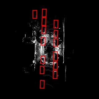
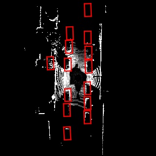
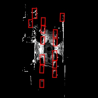
Since AutoFed involves both lidar and radar sensors, there are three possible sensor combinations, i.e., i) lidar + radar (Li + Ra), ii) without radar (w/o Ra), and iii) without lidar (w/o Li). We evaluate the performance of AutoFed  under these three settings, and report the results in Figure 13. The results show that, when the IoU is set to be above 0.5, the median APs achieved by AutoFed are 0.71, 0.57, and 0.12 under the aforementioned three settings. Correspondingly, the median ARs achieved by AutoFed are 0.70, 0.59, and 0.12. The autoencoder employed by AutoFed helps the model to maximize the efficacy of information embedded in either radar or lidar data, and AutoFed exhibits the smallest performance drop compared with the baselines whose performance is drastically impacted by missing modalities. However, since the performance drop of missing modalities stems from the loss of information, even the adoption of an autoencoder cannot totally fill up the performance gap. We have also noticed that the AP and AR of AutoFed are significantly lower in the radar-only mode compared to the other sensor combinations. Upon further investigation, we suspect that this may be because the importance of radar is overshadowed by lidar that provides most of the information used by AutoFed. Specifically, the majority of the vehicles in the dataset are close to the ego vehicle, probably due to the narrow width of the road, and as a result, lidar can detect almost all of these vehicles because they are within its range. This leads to the lower performance of the radar-only mode, as radar is often meant to supplement the lidar sensor for long-range detection.

(a) Average precision.

(b) Average recall.

(c) Lidar + radar.

(d) Missing radar.

(e) Missing lidar.

Figure 13. Different missing modalities.

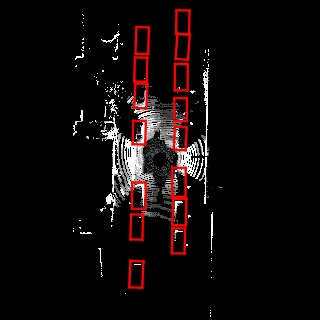
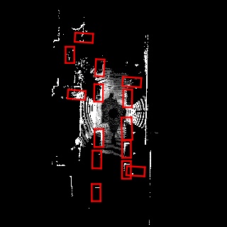
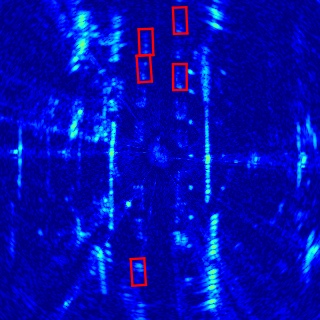
We also show one example of vehicle detection with three sensor combinations in Figure 13. As Figure 13c illustrates, when both lidar and radar are available, AutoFed is able to recognize most of the vehicles on the road. As a comparison, Figure 13d shows that missing radar data affects the detection of vehicles in the further distance, but the nearby vehicles can still be identified. This phenomenon is consistent with the characteristics of the radar sensor, i.e., the radar has an extended range due to better penetration capability while lidar can only obtain a much shorter range due to attenuation caused by in-air particles (Zhao et al., 2020). In addition, we also visualize the case of missing lidar in Figure 13e, where the vehicles in distance can be well detected by the radar. The results clearly demonstrate the complementary sensing capability of radar and lidar.

(a) Average precision.

(b) Average recall.

(c) Foggy.

(d) Rainy.

(e) Snowy.

Figure 14. Different weathers.

4.5.2. Robustness against Adverse Weather Conditions

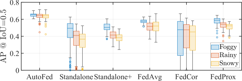
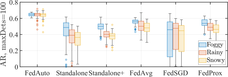
Adverse weather is a realistic but challenging scenario for vehicle detection, which has a negative impact on the sensing capabilities (Kilic et al., 2021). Therefore, we evaluate the performance of AutoFed under different adverse weathers (e.g., foggy, rainy, and snowy). Due to the lack of available datasets collected under adverse weather, we employ the physical models in DEF (Bijelic et al., 2020) and LISA (Kilic et al., 2021) to simulate fog, rain, and snow respectively. Specifically, we set the fog density to 0.05m^-1 in the DEF model and the rate of rain and snow to 30 ​mm/h in the LISA model. Comparing the backgrounds in Figures 14c, 14e, and 14d, while foggy weather attenuates lidar signals and shrinks the field of view, rainy and snowy weathers mainly affect the lidar signals by inducing scattered reflections near the sensor. In particular, the three adverse weather conditions degrade the median AP of AutoFed from 0.71 to 0.65, 0.63, and 0.63, respectively, and degrade the median AR from 0.71 to 0.64, 0.63, and 0.63, respectively. The performance discrepancies among these adverse weathers can be attributed to their different reflectance of lidar signals. Despite the performance degradation, AutoFed exhibits the best generalization when compared with the baselines. The consistently high performance of AutoFed under all adverse weather conditions confirms that the client selection mechanism has allowed the DNN model to effectively incorporate information from unusual circumstances after sufficient training.

4.6. Ablation Study

We evaluate the impact of each module of AutoFed on the model performance. We use AutoFed to train the model for 150 communication rounds, and record the AP in Table 1. Take the AP when IoU is above 0.5 as an example, AutoFed achieves an AP of 0.731, while AutoFed without MCE loss, modality imputation with autoencoder, and client selection obtain the AP of 0.707, 0.692, and 0.542, respectively. One may think that the MCE loss and modality imputation only improves the result by small margins, while the client selection is much more effective in significantly improving performance. However, it is worth noting that both MCE loss and modality imputation are indispensable parts: although the lack of the two can be compensated by client selection (which excludes erroneous gradients) to a certain extent, there still are many heterogeneous scenarios that cannot be addressed by client selection alone, such as those demonstrated in Figures 2 and 3. The integration of MCE loss and modality imputation, together with client selection, can act as “belt and braces” to guarantee the robustness of AutoFed in diversified heterogeneous scenarios.

Table 1. Effects of key AutoFed parts.

	AP
	IoU=0.5:0.9	IoU=0.5	IoU=0.65	IoU=0.8
AutoFed	0.461	0.731	0.698	0.371
w/o MCE	0.405	0.707	0.660	0.212
w/o AE	0.396	0.692	0.657	0.189
w/o CS	0.342	0.542	0.523	0.272

4.7. Hyper-parameter Evaluation

4.7.1. Loss Threshold

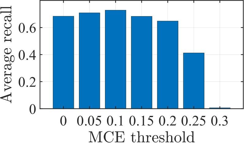
As stated in § 3.3.1, $p_{\mathrm{th}}$ is a threshold above which we believe that the classifier is more trustworthy than the manual annotations. On one hand, when $p_{\mathrm{th}}$ is too small, the MCE loss and traditional CE loss are equivalent, and we cannot exclude incorrect gradients induced by missing annotation boxes. On the other hand, many real backgrounds can be mistakenly excluded if $p_{\mathrm{th}}$ is set too large. Therefore, we evaluate the impact of $p_{\mathrm{th}}$ on the AutoFed performance. As Figure 15a shows, the AP of vehicle detection increases from 0.7 to 0.73 as $p_{\mathrm{th}}$ increases to 0.1. However, the AP rapidly decreases to around 0 at $p_{\mathrm{th}}=0.3$. Likewise, a similar trend can be observed in Figure 15b for AR of the vehicle detection. Overall, Figure 15 offers a guidance for choosing $p_{\mathrm{th}}$.

(a) Average precision.

(b) Average recall.

Figure 15. Impact of the MCE threshold.

4.7.2. The Number of Selected Clients

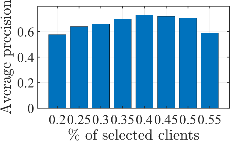
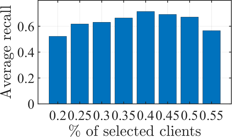
Another hyperparameter that significantly impacts the performance of AutoFed is the number of clients selected for model aggregation. On one hand, a small percentage of selected clients could not fully utilize the diverse data collected by different clients and introduce bias into the federated model. On the other hand, if a very large proportion of the clients are selected, we cannot effectively mitigate the detrimental effect caused by diverged local models. Therefore, the number of selected clients balances the tradeoff between utilizing data and excluding diverged models. As Figure 16a shows, the AP of AutoFed first increases with a greater percentage of selected clients, but starts to drop after the percentage reaches 0.4. The reason is that as the excessive clients are selected for aggregation, the divergence among them will degrade the performance of the federated model. Furthermore, in Figure 16b, it can be seen that AR of AutoFed follows a similar trend as AP, and reaches its peak when the percentage of selected clients is 0.4.

(a) Average precision.

(b) Average recall.

Figure 16. Impact of selected clients percentage.

5. Related Work and Discussion

Recent years have witnessed rapid developments in DNN-based OD methods (Redmon et al., 2016; Liu et al., 2016; Lin et al., 2017; Girshick et al., 2014; Girshick, 2015; Ren et al., 2015). These approaches have been applied to AD (Chen et al., 2017; Yang et al., 2018; Li, 2017; Li et al., 2016). Since most AVs are equipped with multiple sensors (e.g., lidar, radar, and camera), they become technology foundations for the OD systems to fully exploit the multimodal data by sensor fusion. Among various sensor fusion schemes, the combination of lidar and another sensor (e.g., radar or camera) (Ku et al., 2018; Xu et al., 2018; Qi et al., 2018; Chen et al., 2017; Liang et al., 2018; Qian et al., 2021) is a widely-adopted option due to the complements between each other (Geiger et al., 2012; Barnes et al., 2019). One challenge in fusing lidar with other sensors is the unique data structure of lidar, i.e., 3-D point cloud, which is a point set and not compatible with the 2-D matrix in conventional computer vision tasks. One way to overcome this challenge is to employ specially designed DNNs, such as PointNet (Qi et al., 2017), to directly extract features from point clouds and fuse with other sensing data in the feature space (Xu et al., 2018). Another approach is voxelization via transforming the point cloud to 3-D data formats like images, with the height dimension being deemed as image channels. Therefore, the transformed point clouds can be handled by conventional OD-DNNs and fused with other modalities as demonstrated in (Yang et al., 2018; Simon et al., 2019; Zhou and Tuzel, 2018; Luo et al., 2018).

FL (Konečnỳ et al., 2014) is a distributed machine learning paradigm that transfers only model weights instead of explicitly sharing raw data with the central server. AutoFed employs FL to enable data crowdsensing without breaching privacy and incurring unaffordable communication cost on AVs. Despite recent FL applications in classification and regression tasks (Konečnỳ et al., 2014; Li et al., 2020, 2021; Tu et al., 2021; Rehman et al., 2022; So et al., 2022), applying FL to more sophisticated computer vision tasks such as OD (especially vehicle detection) is far from being exploited. In (Jallepalli et al., 2021), the authors investigate the possibility of applying FL to AD applications, and conduct preliminary experiments to verify privacy protection and convergence speed. FedVision (Liu et al., 2020) proposes an online visual OD platform powered by FL, but it focuses more on building and deploying a cloud-based platform, without concerning much on FL-related designs. Fjord (Horvath et al., 2021) claims to target the data heterogeneity in FL, yet it seems to have missed certain complicated aspects, such as annotation and modality heterogeneity tackled in AutoFed.

While different from existing OD proposals by pioneering federated OD on AVs, AutoFed is also the first to take into account the effects of all kinds of multimodal heterogeneity for FL-OD on AVs. However, AutoFed still bears one limitation: it stresses on the FL aspect of crowdsensing, pessimistically assuming a finite number of clients unable to provide complete annotations. In other words, we have not considered positive aspects innate to crowdsensing (Cherian et al., 2016; Wang et al., 2017), such the impact of client incentive (Han et al., 2016b, a). In a future study, we will extend the design goals of AutoFed to include designing proper incentives, in order to expand its user base and attract more AV owners to perform collective learning on distributed AV data and thus guarantee AutoFed service quality.

6. Conclusion

Taking an important step towards full driving automation, we have proposed AutoFed in this paper for federated multimodal vehicle detection. Employing a novel loss function, data imputation technique, and client selection strategy, the AutoFed framework gracefully handles the multimodal data crowdsensed by multiple AV clients, and mines information in the highly heterogeneous data to its maximum, thus releasing its full potential in the vehicle detection task. With extensive experiments under highly heterogeneous scenarios and comparisons with other baselines, we have demonstrated the promising performance of AutoFed in vehicle detection for autonomous driving. We plan to extend AutoFed framework to encompass more sensing modalities, in order to promote its real-life usage and wider acceptance.

Currently, AutoFed targets on FL-driven vehicle detection, but we are planning to apply FL to other out-vehicle sensing tasks, such as pedestrian detection, lane tracking, and environment semantic segmentation. Moreover, modern vehicles are also equipped with in-vehicle sensing modalities to improve user experience, and we believe FL can help improve the performance of deep analytics upon these modalities too. Therefore, we are actively exploring the potential of using FL for full vehicle intelligence, particularly for in-vehicle user monitoring (e.g., (Ding et al., 2020; Zheng et al., 2021; Chen et al., 2021)); this should put us on the right track towards a future with full intelligent transportation.

References

- (1)
- Barnes et al. (2019) Dan Barnes, Matthew Gadd, Paul Murcutt, Paul Newman, and Ingmar Posner. 2019. The Oxford Radar RobotCar Dataset: A Radar Extension to the Oxford RobotCar Dataset. arXiv preprint arXiv: 1909.01300 (2019). https://arxiv.org/pdf/1909.01300
- Bentley (1975) Jon Louis Bentley. 1975. Multidimensional Binary Search Trees used for Associative Searching. Commun. ACM 18, 9 (1975), 509–517.
- Bijelic et al. (2020) Mario Bijelic, Tobias Gruber, Fahim Mannan, Florian Kraus, Werner Ritter, Klaus Dietmayer, and Felix Heide. 2020. Seeing through Fog without Seeing Fog: Deep Multimodal Sensor Fusion in Unseen Adverse Weather. In Proc, of the 33rd IEEE/CVF CVPR. 11682–11692.
- Caesar et al. (2020) Holger Caesar, Varun Bankiti, Alex H Lang, Sourabh Vora, Venice Erin Liong, Qiang Xu, Anush Krishnan, Yu Pan, Giancarlo Baldan, and Oscar Beijbom. 2020. nuScenes: A Multimodal Dataset for Autonomous Driving. In Proc. of the 33rd IEEE/CVF CVPR. 11621–11631.
- Chen et al. (2017) Xiaozhi Chen, Huimin Ma, Ji Wan, Bo Li, and Tian Xia. 2017. Multi-view 3D Object Detection Network for Autonomous Driving. In Proc. of the 30st IEEE/CVF CVPR. 1907–1915.
- Chen et al. (2021) Zhe Chen, Tianyue Zheng, and Jun Luo. 2021. MoVi-Fi: Motion-robust Vital Signs Waveform Recovery via Deep Interpreted RF Sensing. In Proc. of the 27th ACM MobiCom. 392–405.
- Cherian et al. (2016) Jim Cherian, Jun Luo, Hongliang Guo, Shen-Shyang Ho, and Richard Wisbrun. 2016. ParkGauge: Gauging the Occupancy of Parking Garages with Crowdsensed Parking Characteristics. , 92-101 pages.
- Committee et al. (2014) SAE On-Road Automated Vehicle Standards Committee et al. 2014. Taxonomy and Definitions for Terms Related to On-road Motor Vehicle Automated Driving Systems. SAE Standard J 3016 (2014), 1–16.
- De Montjoye et al. (2013) Yves-Alexandre De Montjoye, César A Hidalgo, Michel Verleysen, and Vincent D. Blondel. 2013. Unique in the Crowd: The Privacy Bounds of Human Mobility. Scientific Reports 3, 1 (2013), 1376:1–5.
- Ding et al. (2020) Shuya Ding, Zhe Chen, Tianyue Zheng, and Jun Luo. 2020. RF-Net: A Unified Meta-Learning Framework for RF-enabled One-Shot Human Activity Recognition. In Proc. of the 18th ACM SenSys. 517–530.
- Fallah et al. (2020) Alireza Fallah, Aryan Mokhtari, and Asuman Ozdaglar. 2020. Personalized Federated Learning with Theoretical Guarantees: A Model-Agnostic Meta-Learning Approach. In Proc. of The 34th NeurIPS. 1–12.
- Ganti et al. (2011) Raghu K. Ganti, Fan Ye, and Hui Lei. 2011. Mobile Crowdsensing: Current State and Future Challenges. IEEE Communications Magazine 49, 11 (2011), 32–39.
- Geiger et al. (2012) Andreas Geiger, Philip Lenz, and Raquel Urtasun. 2012. Are We Ready for Autonomous Driving? The KITTI Vision Benchmark Suite. In Proc. of the 25th IEEE/CVF CVPR. IEEE, 3354–3361.
- Girshick (2015) Ross Girshick. 2015. Fast R-CNN. In Proc. of the 29th IEEE ICCV. 1440–1448.
- Girshick et al. (2014) Ross Girshick, Jeff Donahue, Trevor Darrell, and Jitendra Malik. 2014. Rich Feature Hierarchies for Accurate Object Detection and Semantic Segmentation. In Proc. of the 27th IEEE/CVF CVPR. 580–587.
- Han et al. (2016a) Kai Han, He Huang, and Jun Luo. 2016a. Posted Pricing for Robust Crowdsensing. In Proc. of the 17th ACM MobiHoc. 261–270.
- Han et al. (2018) Kai Han, He Huang, and Jun Luo. 2018. Quality-Aware Pricing for Mobile Crowdsensing. IEEE/ACM Transactions on Networking 26, 4 (2018), 1728–1741.
- Han et al. (2016b) Kai Han, Chi Zhang, Jun Luo, Menglan Hu, and Bharadwaj Veeravalli. 2016b. Truthful Scheduling Mechanisms for Powering Mobile Crowdsensing. IEEE Trans. Comput. 65, 1 (2016), 294–307.
- He et al. (2016) Kaiming He, Xiangyu Zhang, Shaoqing Ren, and Jian Sun. 2016. Deep Residual Learning for Image Recognition. In Proc. of the 29th IEEE/CVF CVPR. 770–778.
- Horvath et al. (2021) Samuel Horvath, Stefanos Laskaridis, Mario Almeida, Ilias Leontiadis, Stylianos Venieris, and Nicholas Lane. 2021. Fjord: Fair and Accurate Federated Learning under Heterogeneous Targets with Ordered Dropout. Advances in Neural Information Processing Systems 34 (2021), 12876–12889.
- Intel Corporation (2022) Intel Corporation. 2022. Intel Xeon Gold 6226 Processor. https://www.intel.com/content/www/xa/en/products/sku/193957/intel-xeon-gold-6226-processor-19-25m-cache-2-70-ghz/specifications.html. Accessed: 2022-07-28.
- Jallepalli et al. (2021) Deepthi Jallepalli, Navya Chennagiri Ravikumar, Poojitha Vurtur Badarinath, Shravya Uchil, and Mahima Agumbe Suresh. 2021. Federated Learning for Object Detection in Autonomous Vehicles. In 2021 IEEE Seventh International Conference on Big Data Computing Service and Applications (BigDataService). 107–114.
- Kilic et al. (2021) Velat Kilic, Deepti Hegde, Vishwanath Sindagi, A Brinton Cooper, Mark A Foster, and Vishal M Patel. 2021. Lidar Light Scattering Augmentation (LISA): Physics-based Simulation of Adverse Weather Conditions for 3D Object Detection. arXiv preprint arXiv:2107.07004 (2021).
- Konečnỳ et al. (2014) Jakub Konečnỳ, H Brendan McMahan, Felix X Yu, Peter Richtárik, Ananda Theertha Suresh, and Dave Bacon. 2014. Federated Learning: Strategies for Improving Communication Efficiency. In NIPS Workshop on Private Multi-Party Machine Learning. 1–10.
- Ku et al. (2018) Jason Ku, Melissa Mozifian, Jungwook Lee, Ali Harakeh, and Steven L. Waslander. 2018. Joint 3D Proposal Generation and Object Detection from View Aggregation. In Proc. of IEEE/RSJ IROS. 1–8.
- Li et al. (2021) Ang Li, Jingwei Sun, Xiao Zeng, Mi Zhang, Hai Li, and Yiran Chen. 2021. FedMask: Joint Computation and Communication-efficient Personalized Federated Learning via Heterogeneous Masking. In Proc. of the 19th ACM SenSys. 42–55.
- Li (2017) Bo Li. 2017. 3D Fully Convolutional Network for Vehicle Detection in Point Cloud. In Proc. of IEEE/RSJ IROS. 1513–1518.
- Li et al. (2016) Bo Li, Tianlei Zhang, and Tian Xia. 2016. Vehicle Detection from 3D Lidar using Fully Convolutional Network. arXiv preprint arXiv:1608.07916 (2016).
- Li et al. (2018) Hao Li, Zheng Xu, Gavin Taylor, Christoph Studer, and Tom Goldstein. 2018. Visualizing the Loss Landscape of Neural Nets. Proc. of NeurIPS 31 (2018).
- Li et al. (2020) Tian Li, Anit Kumar Sahu, Manzil Zaheer, Maziar Sanjabi, Ameet Talwalkar, and Virginia Smith. 2020. Federated Optimization in Heterogeneous Networks. Proc. of MLSys 2 (2020), 429–450.
- Liang et al. (2018) Ming Liang, Bin Yang, Shenlong Wang, and Raquel Urtasun. 2018. Deep Continuous Fusion for Multi-sensor 3D Object Detection. In Proc. of the 12th ECCV. 641–656.
- Lin et al. (2017) Tsung-Yi Lin, Priya Goyal, Ross Girshick, Kaiming He, and Piotr Dollár. 2017. Focal Loss for Dense Object Detection. In Proc. of the 31st IEEE ICCV. 2980–2988.
- Lin et al. (2014) Tsung-Yi Lin, Michael Maire, Serge Belongie, James Hays, Pietro Perona, Deva Ramanan, Piotr Dollár, and C Lawrence Zitnick. 2014. Microsoft COCO: Common Objects in Context. In Proc. of the 8th ECCV. 740–755.
- Liu and Niu (2021) Meng Liu and Jianwei Niu. 2021. BEV-Net: A Bird’s Eye View Object Detection Network for LiDAR Point Cloud. In Proc. of IEEE/RSJ IROS. 5973–5980.
- Liu et al. (2016) Wei Liu, Dragomir Anguelov, Dumitru Erhan, Christian Szegedy, Scott Reed, Cheng-Yang Fu, and Alexander C. Berg. 2016. SSD: Single Shot Multibox Detector. In Proc. of the 10th ECCV. 21–37.
- Liu et al. (2020) Yang Liu, Anbu Huang, Yun Luo, He Huang, Youzhi Liu, Yuanyuan Chen, Lican Feng, Tianjian Chen, Han Yu, and Qiang Yang. 2020. Fedvision: An Online Visual Object Detection Platform Powered by Federated Learning. In Proc. of the 34th AAAI, Vol. 34. 13172–13179.
- Luo et al. (2018) Wenjie Luo, Bin Yang, and Raquel Urtasun. 2018. Fast and Furious: Real Time End-to-end 3D Detection, Tracking and Motion Forecasting with a Single Convolutional Net. In Proc. of the 31st IEEE/CVF CVPR. 3569–3577.
- McMahan et al. (2017) Brendan McMahan, Eider Moore, Daniel Ramage, Seth Hampson, and Blaise Aguera y. Arcas. 2017. Communication-efficient Learning of Deep Networks from Decentralized Data. In Proc. of the 20th PMLR AISTATS. 1273–1282.
- Navtech Radar (2022) Navtech Radar. 2022. ClearWay Intelligent Transport Systems Solution. https://navtechradar.com/solutions/clearway/. Accessed: 2022-07-28.
- NVIDIA (2022) NVIDIA. 2022. Jetson TX2 Module. https://developer.nvidia.com/embedded/jetson-tx2. Accessed: 2022-07-28.
- Paszke et al. (2019) Adam Paszke, Sam Gross, Francisco Massa, Adam Lerer, James Bradbury, Gregory Chanan, Trevor Killeen, Zeming Lin, Natalia Gimelshein, Luca Antiga, et al. 2019. PyTorch: An Imperative Style, High-Performance Deep Learning Library. arXiv preprint arXiv:1912.01703 (2019).
- Pearson (1901) Karl Pearson. 1901. On Lines and Planes of Closest Fit to Systems of Points in Space. The London, Edinburgh, and Dublin Philosophical Magazine and Journal of Science 2, 11 (1901), 559–572.
- Petrovskaya and Thrun (2009) Anna Petrovskaya and Sebastian Thrun. 2009. Model based Vehicle Detection and Tracking for Autonomous Urban Driving. Autonomous Robots 26, 2 (2009), 123–139.
- Qi et al. (2018) Charles R Qi, Wei Liu, Chenxia Wu, Hao Su, and Leonidas J. Guibas. 2018. Frustum Pointnets for 3D Object Detection from RGB-D Data. In Proc. of the 31st IEEE/CVF CVPR. 918–927.
- Qi et al. (2017) Charles R. Qi, Hao Su, Kaichun Mo, and Leonidas J. Guibas. 2017. PointNet: Deep Learning on Point Sets for 3D Classification and Segmentation. In Proc. of the 30th IEEE/CVF CVPR. 652–660.
- Qian et al. (2021) Kun Qian, Shilin Zhu, Xinyu Zhang, and Li Erran Li. 2021. Robust Multimodal Vehicle Detection in Foggy Weather using Complementary Lidar and Radar Signals. In Proc. of the 34th IEEE/CVF CVPR. 444–453.
- Redmon et al. (2016) Joseph Redmon, Santosh Divvala, Ross Girshick, and Ali Farhadi. 2016. You Only Look Once: Unified, Real-time Object Detection. In Proc. of the 29th IEEE/CVF CVPR. 779–788.
- Rehman et al. (2022) Yasar Abbas Ur Rehman, Yan Gao, Jiajun Shen, Pedro Porto Buarque de Gusmao, and Nicholas Lane. 2022. Federated Self-supervised Learning for Video Understanding. arXiv preprint arXiv:2207.01975 (2022).
- Ren et al. (2015) Shaoqing Ren, Kaiming He, Ross Girshick, and Jian Sun. 2015. Faster R-CNN: Towards Real-Time Object Detection with Region Proposal Networks. Proc. of The 29th NIPS 28 (2015).
- Scalabel (2022) Scalabel. 2022. Scalabel A Scalable Open-source Web Annotation Tool. https://www.scalabel.ai/. Accessed: 2022-07-28.
- Shaheen and Bouzaghrane (2019) Susan Shaheen and Mohamed Amine Bouzaghrane. 2019. Mobility and Energy Impacts of Shared Automated Vehicles: A Review of Recent Literature. Current Sustainable/Renewable Energy Reports 6, 4 (2019), 193–200.
- Simon et al. (2019) Martin Simon, Karl Amende, Andrea Kraus, Jens Honer, Timo Samann, Hauke Kaulbersch, Stefan Milz, and Horst Michael Gross. 2019. Complexer-YOLO: Real-Time 3D Object Detection and Tracking on Semantic Point Clouds. In Proc. of the 32nd IEEE/CVF CVPR Workshops. 1–10.
- Simonyan and Zisserman (2014) Karen Simonyan and Andrew Zisserman. 2014. Very Deep Convolutional Networks for Large-Scale Image Recognition. arXiv preprint arXiv:1409.1556 (2014).
- So et al. (2022) Jinhyun So, Kevin Hsieh, Behnaz Arzani, Shadi Noghabi, Salman Avestimehr, and Ranveer Chandra. 2022. Fedspace: An Efficient Federated Learning Framework at Satellites and Ground Stations. arXiv preprint arXiv:2202.01267 (2022).
- Tang et al. (2022) Minxue Tang, Xuefei Ning, Yitu Wang, Jingwei Sun, Yu Wang, Hai Li, and Yiran Chen. 2022. FedCor: Correlation-Based Active Client Selection Strategy for Heterogeneous Federated Learning. In Proc. of the 35th IEEE/CVF CVPR. 10102–10111.
- Tesla (2022) Tesla. 2022. Autopilot: Future of Driving. https://www.tesla.com/en_SG/autopilot. Accessed: 2022-07-25.
- Toyota Motor Sales, U.S.A., Inc. (2022) Toyota Motor Sales, U.S.A., Inc. 2022. 2022 Corolla Discover Corolla. Uncover Fun. https://www.toyota.com/corolla/2022/. Accessed: 2022-07-28.
- Tu et al. (2021) Linlin Tu, Xiaomin Ouyang, Jiayu Zhou, Yuze He, and Guoliang Xing. 2021. FedDL: Federated Learning via Dynamic Layer Sharing for Human Activity Recognition. In Proc. of the 19th ACM SenSys. 15–28.
- Uber Technologies Inc. (2022) Uber Technologies Inc. 2022. Self-Driving Perception & Prediction. https://www.uber.com/us/en/atg/research-and-development/perception-and-prediction/. Accessed: 2022-07-25.
- Van Buuren (2018) Stef Van Buuren. 2018. Flexible Imputation of Missing Data. CRC press.
- Vaswani et al. (2017) Ashish Vaswani, Noam Shazeer, Niki Parmar, Jakob Uszkoreit, Llion Jones, Aidan N. Gomez, Łukasz Kaiser, and Illia Polosukhin. 2017. Attention is All You Need. Proc. of the 31st NIPS 30 (2017), 1–11.
- Velodyne Lidar, Inc. (2022) Velodyne Lidar, Inc. 2022. HDL-32E High Resolution Real-Time 3D Lidar Sensor. https://velodynelidar.com/products/hdl-32e/. Accessed: 2022-07-28.
- Vergara-Laurens et al. (2016) Idalides J. Vergara-Laurens, Luis G. Jaimes, and Miguel A. Labrador. 2016. Privacy-preserving Mechanisms for Crowdsensing: Survey and Research Challenges. IEEE Internet of Things Journal 4, 4 (2016), 855–869.
- Wang et al. (2019) Jin Wang, Jun Luo, Sinno Jialin Pan, and Aixin Sun. 2019. Learning-Based Outdoor Localization Exploiting Crowd-Labeled WiFi Hotspots. IEEE Transactions on Mobile Computing 18, 4 (2019), 896–909.
- Wang et al. (2017) Jin Wang, Nicholas Tan, Jun Luo, and Sinno Jialin Pan. 2017. WOLoc: WiFi-only outdoor localization using crowdsensed hotspot labels. In Proc. of the 36th IEEE INFOCOM. 1–9.
- Waymo (2022) Waymo. 2022. We’re building the World’s Most Experienced Driver. https://waymo.com/?ncr. Accessed: 2022-07-25.
- Waze Mobile Limited (2022) Waze Mobile Limited. 2022. Waze: Navigation & Live Traffic. (https://www.waze.com/. Accessed: 2022-07-28.
- Wei et al. (2020) Xi Wei, Tianzhu Zhang, Yan Li, Yongdong Zhang, and Feng Wu. 2020. Multi-modality Cross Attention Network for Image and Sentence Matching. In Proc. of the 33rd IEEE/CVF CVPR. 10941–10950.
- Wu, Yuxin and Kirillov, Alexander and Massa, Francisco and Lo, Wan-Yen and Girshick, Ross (2022) Wu, Yuxin and Kirillov, Alexander and Massa, Francisco and Lo, Wan-Yen and Girshick, Ross. 2022. Detectron2. https://github.com/facebookresearch/detectron2. Accessed: 2022-07-25.
- Xu et al. (2018) Danfei Xu, Dragomir Anguelov, and Ashesh Jain. 2018. PointFusion: Deep Sensor Fusion for 3D Bounding Box Estimation. In Proc. of the 31st IEEE/CVF CVPR. 244–253.
- Yang et al. (2018) Bin Yang, Wenjie Luo, and Raquel Urtasun. 2018. PIXOR: Real-time 3D Object Detection from Point Clouds. In Proc. of the 31st IEEE/CVF CVPR. 7652–7660.
- Yang et al. (2012) Dejun Yang, Guoliang Xue, Xi Fang, and Jian Tang. 2012. Crowdsourcing to Smartphones: Incentive Mechanism Design for Mobile Phone Sensing. In Proc. of the 18th ACM MobiCom. 173–184.
- Yu and Liu (2019) Peihua Yu and Yunfeng Liu. 2019. Federated Object Detection: Optimizing Object Detection Model with Federated Learning. In Proceedings of the 3rd International Conference on Vision, Image and Signal Processing. 1–6.
- Zhang et al. (2014) Chi Zhang, Jun Luo, and Jianxin Wu. 2014. A Dual-Sensor Enabled Indoor Localization System with Crowdsensing Spot Survey. In Proc. of the 10th IEEE/ACM DCOSS. 75–82.
- Zhang et al. (2015) Chi Zhang, Kalyan P. Subbu, Jun Luo, and Jianxin Wu. 2015. GROPING: Geomagnetism and cROwdsensing Powered Indoor NaviGation. IEEE Transactions on Mobile Computing 14, 2 (2015), 387–400.
- Zhao et al. (2020) Jian Zhao, Yaxin Li, Bing Zhu, Weiwen Deng, and Bohua Sun. 2020. Method and Applications of LiDAR Modeling for Virtual Testing of Intelligent Vehicles. IEEE Transactions on Intelligent Transportation Systems 22, 5 (2020), 2990–3000.
- Zheng et al. (2021) Tianyue Zheng, Zhe Chen, Jun Luo, Lin Ke, Chaoyang Zhao, and Yaowen Yang. 2020. SiWa: See into Walls via Deep UWB radar. In Proc. of the 27th ACM MobiCom. 323–336.
- Zheng et al. (2021) Tianyue Zheng, Zhe Chen, Chao Cai, Jun Luo, and Xu Zhang. 2020. V2iFi: in-Vehicle Vital Sign Monitoring via Compact RF Sensing. In Proc. of the 20th ACM UbiComp. 70:1–27.
- Zhou and Tuzel (2018) Yin Zhou and Oncel Tuzel. 2018. VoxelNet: End-to-End Learning for Point Cloud based 3D Object Detection. In Proc. of the 31st IEEE/CVF CVPR. 4490–4499.