Quantum Computing Provides Exponential Regret Improvement in Episodic Reinforcement Learning

Abstract

In this paper, we investigate the problem of episodic reinforcement learning with quantum oracles for state evolution. To this end, we propose an Upper Confidence Bound (UCB) based quantum algorithmic framework to facilitate learning of a finite-horizon MDP. Our quantum algorithm achieves an exponential improvement in regret as compared to the classical counterparts, achieving a regret of $\tilde{\mathcal{O}}(1)$ as compared to $\tilde{\mathcal{O}}(\sqrt{K})$ , $K$ being the number of training episodes. In order to achieve this advantage, we exploit efficient quantum mean estimation technique that provides quadratic improvement in the number of i.i.d. samples needed to estimate the mean of sub-Gaussian random variables as compared to classical mean estimation. This improvement is a key to the significant regret improvement in quantum reinforcement learning. We provide proof-of-concept experiments on various RL environments that in turn demonstrate performance gains of the proposed algorithmic framework.

1 Introduction

Quantum Machine Learning (QML) is an emerging domain built at the confluence of quantum information processing and Machine Learning (ML) (Saggio et al., 2021). A noteworthy volume of prior works in QML demonstrate how quantum computers could be effectively leveraged to improve upon classical results pertaining to classification/regression based predictive modeling tasks (Aïmeur et al., 2013; Rebentrost et al., 2014; Arunachalam and de Wolf, 2017). While the efficiency of QML frameworks have been shown on conventional supervised/unsupervised ML use cases, how similar improvements could be translated to Reinforcement Learning (RL) tasks have gained significant attention recently and is the focus of this paper.

Traditional RL tasks comprise of an agent interacting with an external environment attempting to learn its configurations, while collecting rewards via actions and state transitions (Sutton and Barto, 2018). RL techniques have been credibly deployed at scale over a variety of agent driven decision making industry use cases, e.g., autonomous navigation in self-driving cars (Al-Abbasi et al., 2019), recommendation systems in e-commerce websites (Rohde et al., 2018), and online gameplay agents such as AlphaGo (Silver et al., 2017). Given the wide applications, this paper aims to study if quantum computing can help further improve the performance of reinforcement learning algorithms. This paper considers an episodic setup, where the learning occurs in episodes with a finite horizon. The performance measure for algorithm design is the regret of agent’s rewards (Mnih et al., 2016; Cai et al., 2020), which measures the gap in the obtained rewards by the Algorithm and the optimal algorithm. A central idea in RL algorithms is the notion of exploration-exploitation trade-off, where agent’s policy is partly constructed on its experiences so far with the environment as well as injecting a certain amount of optimism to facilitate exploring sparsely observed policy configurations (Kearns and Singh, 2002; Jin et al., 2020). In this context, we emphasize that our work adopts the well-known Value Iteration (VI) technique which combines empirically updating state-action policy model with Upper Confidence Bound (UCB) based strategic exploration (Azar et al., 2017).

In this paper, we show an exponential improvement in the regret of reinforcement learning. The key to this improvement is that quantum computing allows for improved mean estimation results over classical algorithms (Brassard et al., 2002; Hamoudi, 2021). Such mean estimators feature in very recent studies of quantum bandits (Wang et al., 2021b), quantum reinforcement learning (Wang et al., 2021a), thereby leading to noteworthy convergence gains. In our proposed framework, we specifically incorporate a quantum information processing technique that improves non-asymptotic bounds of conventional empirical mean estimators which was first demonstrated in (Hamoudi, 2021). In this regard, it is worth noting that a crucial novelty pertaining to this work is carefully engineering agent’s interaction with the environment in terms of collecting classical and quantum signals. We further note that one of the key aspects of analyzing reinforcement learning algorithms is the use of Martingale convergence theorems, which is incorporated through the stochastic process in the system evolution. Since there is no result on improved Martingale convergence results in quantum computing so far (to the best of our knowledge), this work does a careful analysis to approach the result without use of Martingale convergence results.

Given the aforementioned quantum setup in place, this paper attempts to address the following: Can we design a quantum VI Algorithm that can improve classical regret bounds in episodic RL setting?

This paper answers the question in positive. The key to achieve such quantum advantage is the use of quantum environment that provides more information than just an observation of the next state. This enhanced information is used with quantum computing techniques to obtain efficient reget bounds in this paper.

To this end, we summarize the major contributions of our work as follows:

1. We present a novel quantum RL architecture that helps exploit the quantum advantage in episodic reinforcement learning.

2. We propose QUCB-VI, which builds on the classical UCB-VI algorithm (Azar et al., 2017), wherein we carefully leverage available quantum information and quantum mean estimation techniques to engineer computation of agent’s policy.

3. We perform rigorous theoretical analysis of the proposed framework and characterize its performance in terms of regret accumulated across $K$ episodes of agent’s interaction with the unknown Markov Decision Process (MDP) environment. More specifically, we show that QUCB-VI incurs $\tilde{\mathcal{O}}(1)$ regret. We note that our algorithm provides a faster convergence rate in comparison to classical UCB-VI which accumulates $\tilde{\mathcal{O}}(\sqrt{K})$ regret, where $K$ is the number of training episodes.

4. We conduct thorough experimental analysis of QUCB-VI (algorithm 1) and compare against baseline classical UCB-VI algorithm on a variety of benchmark RL environments. Our experimental results reveals QUCB-VI’s performance improvements in terms of regret growth over baseline.

The rest of the paper is organized as follows. In Section 2, we present a brief background of key existing literature pertaining to classical RL, as well as discuss prior research conducted in development of quantum mean estimation techniques and quantum RL methodologies relevant to our work. In Section 3, we mathematically formulate the problem of episodic RL in a finite horizon unknown MDP with the use of quantum oracles in the environment. In Section 4, we describe the proposed QUCB-VI Algorithm while bringing out key differences involving agent’s policy computations as compared to classical UCB-VI. Subsequently, we provide the formal analysis of regret for the proposed algorithm in Section 5. In Section 6, we report our results of experimental evaluations performed on various RL environments for the proposed algorithm and classical baseline method. Section 7 concludes the paper.

2 Background and Related Work

Classical reinforcement learning:  In the context of classical RL, an appreciable segment of prior research focus on obtaining theoretical results in tabular RL, i.e., agent’s state and action spaces are discrete (Sutton and Barto, 2018). Several existing methodologies guarantee sub-linear regret in this setting via leveraging optimism in the face of uncertainty (OFU) principle (Lai et al., 1985), to strategically balance exploration-exploitation trade-off (Osband et al., 2016; Strehl et al., 2006). Furthermore, on the basis of design requirements and problem specific use cases, such algorithms have been mainly categorized as either model-based  (Auer et al., 2008; Dann et al., 2017) or model-free  (Jin et al., 2018; Du et al., 2019). In the episodic tabular RL problem setup, the optimal regret of $\tilde{\mathcal{O}}(\sqrt{K})$ ($K$ is the number of episodes) have been studied for both model-based as well as model-free learning frameworks (Azar et al., 2017; Jin et al., 2018). In this paper, we study model-based algorithms and derive $\tilde{\mathcal{O}}(1)$ regret with the use of quantum environment.

Quantum Mean Estimation:   Mean estimation is a statistical inference problem in which samples are used to produce an estimate of the mean of an unknown distribution. The improvement in sample complexity for mean estimation using quantum computing has been widely studied (Grover, 1998; Brassard et al., 2002, 2011). In (Montanaro, 2015), a quantum information assisted Monte-Carlo Algorithm was proposed which achieves an asymptotic near-quadratic faster convergence over its classical baseline. In this paper, we use the approach in (Hamoudi, 2021) for the mean estimation of quantum random variables. We first describe the notion of random variable and corresponding extension to quantum random variable.

Definition 1 (Random Variable)

A finite random variable is a function $X:\Omega\to E$ for some probability space $(\Omega,P)$, where $\Omega$ is a finite sample set, $P:\Omega\to[0,1]$ is a probability mass function and $E\subset\mathbb{R}$ is the support of $X$. As is customary, we will often omit to mention $(\Omega,P)$ when referring to the random variable $X$.

The notion is extended to a quantum random variable (or q.r.v.) as follows.

Definition 2 (Quantum Random Variable)

A q.r.v. is a triple $(\mathcal{H},U,M)$ where $\mathcal{H}$ is a finite-dimensional Hilbert space, $U$ is a unitary transformation on $\mathcal{H}$, and $M=\{M_{x}\}_{x\in E}$ is a projective measurement on $\mathcal{H}$ indexed by a finite set $E\subset\mathbb{R}$. Given a random variable $X$ on a probability space $(\Omega,P)$, we say that a q-variable $(\mathcal{H},U,M)$ generates $X$ when,

• $\mathcal{H}$ is a finite-dimensional Hilbert space with some basis $\{|\omega\rangle\}_{\omega\in\Omega}$ indexed by $\Omega$.

• $U$ is a unitary transformation on $\mathcal{H}$ such that $U|\mathbf{0}\rangle=\sum_{\omega\in\Omega}\sqrt{P(\omega)}|\omega\rangle$.

• $M=\{M_{x}\}_{x}$ is the projective measurement on $\mathcal{H}$ defined by $M_{x}=\sum_{\omega:X(\omega)=x}|\omega\rangle\langle\omega|$.

We now define the notion of a quantum experiment. Let $(\mathcal{H},U,M)$ be a q.r.v. that generates $X$. With abuse of notations, we call $X$ as the q.r.v. even though the actual q.r.v. is the $(\mathcal{H},U,M)$ that generates $X$. We define a quantum experiment as the process of applying any of the unitaries $U$, their inverses or their controlled versions, or performing a measurement according to $M$. We also assume an access to the quantum evaluation oracle $|\omega\rangle|0\rangle\to|\omega\rangle|X(\omega)\rangle$. Using this quantum oracle, the quantum mean estimation result can be stated as follows.

Lemma 1 (Sub-Gaussian estimator (Hamoudi, 2021))

Let $X$ be a q.r.v. with mean $\mu$ and variance $\sigma^{2}$. Given $n$ i.i.d. samples of q.r.v. $X$ and a real $\delta\in(0,1)$ such that $n>\log(1/\delta)$, a quantum algorithm SubGaussEst$(X,n,\delta)$ (please refer to algorithm 2 in (Hamoudi, 2021)) outputs a mean estimate $\hat{\mu}$ such that,

$$P\left[|\hat{\mu}-\mu|\leq\frac{\sigma\log(1/\delta)}{n}\right]\geq 1-\delta.$$ (1)

The algorithm performs $O(n\log^{3/2}(n)\log\log(n))$ quantum experiments.

We note that this result achieves the mean estimation error of $1/n$ in contrast to $1/\sqrt{n}$ for the classical mean estimation, thus providing a quadratic reduction in the number of i.i.d. samples needed for same error bound.

Quantum reinforcement learning:  Recently, quantum mean estimation techniques have been applied with favorable theoretical convergence speed-ups for Quantum multi-armed bandits (MAB) problem setting (Casalé et al., 2020; Wang et al., 2021b; Lumbreras et al., 2022). However, bandits do not have the notion of state evolution like in reinforcement learning. Further, quantum reinforcement learning has been studied in (Paparo et al., 2014; Dunjko et al., 2016, 2017; Jerbi et al., 2021; Dong et al., 2008), while these works do not study the regret performance. The theoretical regret performance has been recently studied in (Wang et al., 2021b), where a generative model is assumed and sample complexity guarantees are derived for discounted infinite horizon setup. In contrast, our work does not consider discounted case, and we don’t assume a generative model. This paper demonstrates the quantum speedup for episodic reinforcement learning.

3 Problem Formulation

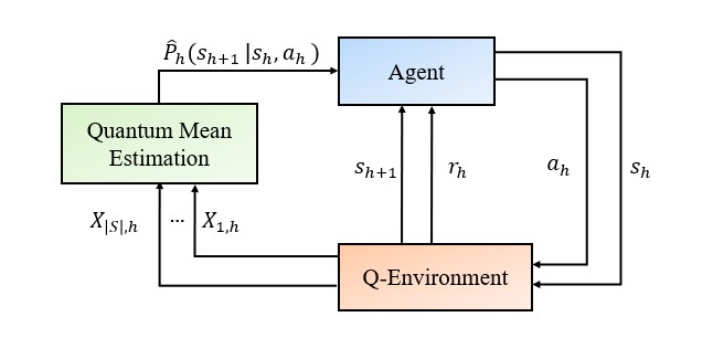
Figure 1: Quantum episodic reinforcement learning architecture depicting agent-environment interaction at round $h$.

We consider episodic reinforcement learning in a finite horizon Markov Decision Process (Agarwal et al., 2019) given by a tuple $\left(\mathcal{S},\mathcal{A},H,\{P_{h}\}_{h\in[0,H-1]},\{r_{h}\}_{h\in[0,H-1]}\right)$, where $\mathcal{S}$ and $\mathcal{A}$ are the state and the action spaces with cardinalities $S$ and $A$, respectively, $H\in\mathbb{N}$ is the episode length, $P_{h}(s^{\prime}|s,a)\in[0,1]$ is the probability of transitioning to state $s^{\prime}$ from state $s$ provided action $a$ is taken at step $h$ and $r_{h}(s,a)\in[0,1]$ is the immediate reward associated with taking action $a$ in state $s$ at step $h$. In our setting, we denote an episode by the notation $k$, and every such episode comprises of $H$ rounds of agent’s interaction with the learning environment. In our problem setting, we assume an MDP with a fixed start state $s_{0}$, where at the start of each new episode the state is reset to $s_{0}$. We note that the results can be easily extended to the case where starting state is sampled from some distribution. This is because we can have a dummy state $s_{0}$ which transitions to the next state $s_{1}$ coming from this distribution, independent of action, and having a reward of $0$.

We encapsulate agent’s interaction with the unknown MDP environment via the architecture as presented in Fig. 1. At an arbitrary time step $h$, given a state $s_{h}$ and action $a_{h}$, the environment gives the reward $r_{h}$ and next state $s_{h+1}$. Furthermore, we highlight that in our proposed architecture this set of signals i.e., $\{s_{h},a_{h},r_{h},s_{h+1}\}$ are collected at the agent as classical information. Additionally, our architecture facilitates availability of $S$ quantum random variables (q.r.v.) ($X_{1,h},\cdots,X_{S,h}$) at the agent’s end, wherein q.r.v. $X_{i,h}$ generates the random variable $\mathbf{1}\left\{s_{h+1}=i\right\}$. This q.r.v. corresponds to the Hilbert space with basis vectors $|0\rangle$ and $|1\rangle$ and the unitary transformation, given as follows:

$$U|\mathbf{0}\rangle= \sqrt{1-P_{h}(s_{h+1}=i|s_{h},~{}a_{h})}|0\rangle$$

$$~{}~{}~{}+\sqrt{P_{h}(s_{h+1}=i|s_{h},~{}a_{h})}|1\rangle.$$ (2)

We note that these q.r.v.’s can be generated by using a quantum next state from the environment which is given in form of the basis vectors for $S$ states as $|10\cdots 0>$ with $S$ qubits for first state and so on till $|0\cdots 01>$ for the last state. Thus, the overall quantum next state is the superposition of these $S$ states with the amplitudes as $\sqrt{P_{h}(s_{h+1}=1|s_{h},~{}a_{h})},\cdots,\sqrt{P_{h}(s_{h+1}=S|s_{h},~{}a_{h})}$, respectively. The $S$ q.r.v.’s correspond to the $S$ qubits in this next quantum state. Further, the next state can be obtained as a measurement of this joint next state superposition. Thus, assuming that the quantum environment can generate multiple copies of the next state superposition, all the $S$ q.r.v.’s and the next state measurement can be obtained.

We note that the agent does not know $\{P_{h}\}_{h\in[0,H-1]}$, which needs to be estimated in the model-based setup. In order to estimate this, we will use the quantum mean estimation approach. This approach needs as quantum evaluation oracle $|\omega\rangle|0\rangle\to|\omega\rangle|\mathbf{1}\left\{s_{h+1}=\omega\right\}\rangle$ for $\omega\in\{0,1\}$. In Section 4, we provide more details on how the aforementioned set of quantum indicator variables i.e., $\{{X_{s^{\prime},h}}\}_{s^{\prime}\in\mathcal{S}}$ are fed to a specific quantum mean estimation procedure to obtain the transition probability model.

Based on the observations, the agent needs to determine a policy $\pi_{h}$ which determines action $a_{h}$ given state $s_{h}$. For given policy $\pi$ and $h\in\{0,\cdots,H-1\}$, we define the value function $V_{h}^{\pi}:\mathcal{S}\rightarrow\mathbb{R}$ as

$$V_{h}^{\pi}(s)=\mathbb{E}\left[\sum_{t=h}^{H-1}r_{h}\left(s_{t},a_{t}\right)\mid\pi,~{}s_{h}=s\right],$$ (3)

where the expectation is with respect to the randomness of the trajectory, that is, the randomness in state transitions and the stochasticity of $\pi$. Similarly, the state-action value (or $Q$-value) function $Q_{h}^{\pi}:\mathcal{S}\times\mathcal{A}\rightarrow\mathbb{R}$ is defined as

$$Q_{h}^{\pi}(s,a)=\mathbb{E}\left[\sum_{t=h}^{H-1}r_{h}\left(s_{t},a_{t}\right)\mid\pi,s_{h}=s,a_{h}=a\right].$$ (4)

We also use the notation $V^{\pi}(s)=V_{0}^{\pi}(s)$. Given a state s, the goal of the agent is to find a policy $\pi^{*}$ that maximizes the value, i.e., the optimization problem the agent seeks to solve is:

$$\max_{\pi}~{}V^{\pi}(s).$$ (5)

Define $Q_{h}^{\star}(s,a)=\sup_{\pi\in\Pi}~{}Q_{h}^{\pi}(s,a)$ and $V_{h}^{\star}(s)=\sup_{\pi\in\Pi}~{}V_{h}^{\pi}(s)$. The agent aims to minimize the expected cumulative regret incurred across $K$ episodes:

$$\texttt{Regret:}~{}\mathbb{E}\big{[}KV^{*}(s_{0})-\sum_{k=0}^{K-1}\sum_{h=0}^{H-1}r(s_{h}^{k},a_{h}^{k})\big{]}.$$ (6)

In the following section, we describe the proposed algorithm and analyze its regret in Section 5.

4 Algorithmic Framework

In this section, we describe in detail our quantum information assisted algorithmic framework to perform learning of unknown MDP under finite horizon episodic RL setting. In particular, we propose a quantum algorithm that incorporates model-based episodic RL procedure originally proposed in the classical setting (Azar et al., 2017; Agarwal et al., 2019). In algorithm 1, we present Quantum Upper Confidence Bound - Value Iteration (QUCB-VI) Algorithm which takes number of episodes $K$, length of an episode $H$ and confidence parameter $\delta$ as inputs. In the very first step, the count of visitations corresponding to every state-action pair $(s,a)\in\mathcal{S}\times\mathcal{A}$ are initialized to 0. Subsequently, at the beginning of each episode $K$, the value function estimates for the entire state-space $\mathcal{S}$, i.e., $\{\widehat{V}_{H}^{k}(s)\}_{s\in\mathcal{S}}$ are set to 0.

Next, for each time instant up to $H-1$, we update the transition probability model. Here, we utilize the set of quantum random variable (q.r.v.) $\{X_{s^{\prime},h}^{k}\}_{s^{\prime}\in\mathcal{S}}$ as introduced in our quantum RL architecture presented in Figure 1. Recall that the elements of $\{X_{s^{\prime},h}^{k}\}_{s^{\prime}\in\mathcal{S}}$ are defined at each time step $h$ during episode $k$ as follows:

$$X_{s^{\prime},h}^{k}\triangleq\mathrm{1}[s_{h+1}^{k}=s^{\prime}].$$ (7)

We define $N_{h}^{k}(s,a)$ as the number of times $(s,a)$ is visited before episode $k$. More formally, we have

$$N_{h}^{k}(s,a)=\sum_{i=0}^{k-1}\mathbf{1}\big{[}(s_{h}^{i},a_{h}^{i})=(s,a)\big{]}.$$ (8)

Algorithm 1 QUCB-VI

1:Inputs: $K$, $H$, $\delta\in(0,1]$.

2:Set ${N}_{h}^{1}(s,a)\leftarrow 0,~{}\forall~{}s\in\mathcal{S},~{}a\in\mathcal{A},~{}h\in[0,H-1])$.

3:for $k=1,\dots,K$ do

4:     Set $\widehat{V}_{H}^{k}(s)\leftarrow 0,~{}\forall s\in\mathcal{S}$.

5:     for $h=H-1,\dots,1,0$ do.

6:         Set $\{\hat{P}_{h}^{k}(s^{\prime}|s,a)\}_{s,a,s^{\prime})\in\mathcal{S}\times\mathcal{A}\times\mathcal{S}}$ via Eq. (9).

7:         Set $b_{h}^{k}(s,a)\leftarrow\frac{\log(SAHK/\delta)}{N_{h}^{k}(s,a)}$.

8:         Set $\{\widehat{Q}_{h}^{k}(s,a)\}_{s\in\mathcal{S},a\in\mathcal{A}}$ via Eq. (10).

9:         Set $\{\widehat{V}_{h}^{k}(s)\}_{s\in\mathcal{S}}$ via Eq. (11).

10:     end for

11:     Set policies $\{\pi_{h}^{k}(s)\}_{s\in\mathcal{S},h\in[0,H-1]}$ using Eq. (12).

12:      Get Trajectory $\{s_{h}^{k},a_{h}^{k},r_{h}^{k},s_{h+1}^{k}\}_{h=0}^{H-1}$ via $\{\pi_{h}^{k}\}_{h=0}^{H-1}$.

13:     Set $\{{N}_{h}^{k+1}(s,a)\}_{s\in\mathcal{S},a\in\mathcal{A},h\in[0,H-1]}$ via Eq. (8).

14:end for

${N}_{h}^{k}(s,a)$ indicates the number of samples obtained for $(s,a)$ in the past which will help in efficient averaging to estimate the transition probabilities. With the formulation of q.r.v. $\{X_{s^{\prime},h}^{k}\}_{s^{\prime}\in\mathcal{S}}$ in place, we update the transition probability model elements, i.e., $\{\hat{P}_{h}^{k}(s^{\prime}|s,a)\}_{(s,a,s^{\prime})\in\mathcal{S}\times\mathcal{A}\times\mathcal{S}}$, in step 6 of algorithm 1. To get the estimate of $\hat{P}_{h}^{k}(s^{\prime}|s,a)$, we use the ${N}_{h}^{k}(s,a)$ q.r.v.’s $X_{s^{\prime},h}^{k}$ for all past $k$. Thus, $\hat{P}_{h}^{k}(s^{\prime}|s,a)$ is estimated as:

$$\hat{P}_{h}^{k}(s^{\prime}|s,a)\leftarrow~{}\texttt{SubGaussEst}(X_{s^{\prime},h}^{k},{N}_{h}^{k}(s,a),\delta),$$ (9)

where subroutine SubGaussEst as presented in Algorithm 2 of (Hamoudi, 2021) performs mean estimation of q.r.v. $X_{s^{\prime},h}^{k}$ given ${N}_{h}^{k}(s,a)$ collection of samples and confidence parameter $\delta$. We emphasize that step 6 in Algorithm 1 brings out the key change w.r.t. classical UCB-VI via carefully estimating mean of quantum information collected by agent via interaction with the unknown MDP environment. In step 7, we set the reward bonus i.e., $b_{h}^{k}(s,a)$ which resembles a Bernstein-style UCB bonus, essentially inducing optimism in the learnt model. Consequently, step 8-9 compute estimates of $\{{Q}_{h}^{k}(s,a)\}_{s\in\mathcal{S},a\in\mathcal{A}},~{}\{\widehat{V}_{h}^{k}(s)\}_{s\in\mathcal{S}}$ by adopting the following Value Iteration based updates at time step $h$:

$$\widehat{Q}_{h}^{k}(s,a)\leftarrow\min\{H,{r}_{h}^{k}(s,a)+\langle\widehat{V}_{h+1}^{k},\widehat{P}_{h}^{k}\left(\cdot|s,a\right)\rangle$$

$$\hskip 85.35826pt+b_{h}^{k}(s,a)\},$$ (10)

$$\widehat{V}_{h}^{k}(s)\leftarrow\underset{a\in\mathcal{A}}{\max}~{}\widehat{Q}_{h}^{k}(s,a).$$ (11)

This Value Iteration procedure (i.e., inner loop consisting of steps 6-9) is executed for $H$ time steps thereby generating a collection of $H$ policies $\{\pi_{h}^{k}(s)\}_{s\in\mathcal{S},h\in[0,H-1]}$ calculated for each pair of $(s,h)$ in step 11 as:

$$\pi_{h}^{k}(s)\leftarrow\underset{a\in\mathcal{A}}{\arg\max}~{}\widehat{Q}_{h}^{k}(s,a),$$ (12)

Next, using the updated policies i.e., $\{\pi_{h}^{k}(s)\}_{s\in\mathcal{S},h\in[0,H-1]}$ which are based on observations recorded till episode $k-1$, the agent collects a new trajectory of $H$ tuples pertaining to episode $k$ i.e., $\{s_{h}^{k},a_{h}^{k},r_{h}^{k},s_{h+1}^{k}\}_{h=0}^{H-1}$ in step 12 starting from initial state reset to $s_{0}$. Finally, the frequency of agent’s visitation to all state action pairs at every time step $h$ over the $k$ episodes i.e., $\{{N}_{h}^{k+1}(s,a)\}_{s\in\mathcal{S},a\in\mathcal{A},h\in[0,H-1]}$ are updated in step 13. Consequently, algorithm 1 triggers a new episode of agent’s interaction with the unknown MDP environment.

5 Regret Results for the Proposed Algorithm

5.1 Main Result: Regret Bound for QUCB-VI

In Theorem 1, we present the cumulative regret collected upon deploying QUCB-VI in an unknown MDP environment $\mathcal{M}$ (please refer to Section 3 for definition of MDP) over a finite horizon of $K$ episodes.

Theorem 1

In an unknown MDP environment $\mathcal{M}\triangleq\left(\mathcal{S},\mathcal{A},H,\{P_{h}\}_{h\in[0,H-1]},\{r_{h}\}_{h\in[0,H-1]}\right)$, the regret incurred by QUCB-VI (algorithm 1) across $K$ episodes is bounded as follows:

$$\mathbb{E}\Big{[}\sum_{k=0}^{K-1}\big{(}V^{*}(s_{0}) -V^{\pi^{k}}(s_{0})\big{)}\Big{]}$$

$$\leq O(H^{2}S^{2}A\log^{2}(SAH^{2}K^{2})).$$ (13)

The result obtained via Eq. (13) in Theorem 1 brings out the key advantage of the proposed framework in terms of accelerating the regret convergence rate to $\tilde{\mathcal{O}}(1)$ against the classical result of $\tilde{\mathcal{O}}(\sqrt{K})$ (Azar et al., 2017).

In order to prove Theorem 1, we present the following auxiliary mathematical results in the ensuing subsections: bound for probability transition model error pertaining to every state-action pair (section 5.2); optimism exhibited by the learnt model understood in terms of value functions of the states (section 5.3); a supporting result that bounds inverse frequencies of state-action pairs over the entire observed trajectory (section 5.4). Subsequently, we utilize these aforementioned theoretical results to prove Theorem 1 in section 5.5.

5.2 Probability Transition Model Error for state-action pairs

Lemma 2

For $k\in\{0,\ldots,{K}-1\}$, $s\in\mathcal{S}$, $a\in\mathcal{A}$, $h\in\{0,\ldots,H-1\}$, for any $f:\mathcal{S}\rightarrow[0,H]$, execution of QUCB-VI (algorithm 1) guarantees that the following holds with probability at least $1-\delta$:

$$\Big{|}\Big{(}\hat{P}_{h}^{k}(\cdot|s,a)-{P}_{h}(\cdot|s,a)\Big{)}^{T}f\Big{|}\leq\frac{HSL}{N_{h}^{k}(s,a)},$$ (14)

where $L\triangleq{\log(SAHK/\delta)}$ and $\{N_{h}^{k}(s,a)$, $\hat{P}_{h}^{k}(s^{\prime}|s,a)\}$ are defined in Eq. (8), (9).

Proof  To prove the claim in Eq. (14), we consider an arbitrary tuple $(s,a,k,h,f)$ and obtain the following:

$$\Big{|}\Big{(}\hat{P}_{h}^{k}(\cdot|s,a) -{P}_{h}(\cdot|s,a)\Big{)}^{T}f\Big{|}$$

$$\leq\sum_{s^{\prime}\in\mathcal{S}}f(s^{\prime})|\hat{P}_{h}^{k}(s^{\prime}|s,a)-{P}_{h}(s^{\prime}|s,a)|,$$ (15)

$$\leq H\sum_{s^{\prime}\in\mathcal{S}}|\underbrace{\hat{P}_{h}^{k}(s^{\prime}|s,a)-{P}_{h}(s^{\prime}|s,a)}_{\text{(a)}}|,$$ (16)

where Eq. (16) is due to the definition of $f(\cdot)$ as presented in the lemma statement. Next, in order to analyze (a) in Eq. (16), we note the definition of $X_{s^{\prime},h}^{k}$ presented in Eq. (7) as an indicator q.r.v allows us to write:

$$\hat{P}_{h}^{k}(s^{\prime}|s,a)=\mathbb{E}_{q,\hat{P}_{h}^{k}}[X_{s^{\prime},h}^{k}|s,a],$$ (17)

$${P}_{h}(s^{\prime}|s,a)=\mathbb{E}_{q,{P}_{h}}[X_{s^{\prime},h}^{k}|s,a].$$ (18)

Using the fact that $X_{s^{\prime},h}^{k}$ is a q.r.v. allows us to directly apply Lemma 1, thereby further bounding (a) in Eq. (16) with probability at least $1-\delta$ as follows:

$$|\hat{P}_{h}^{k}(s^{\prime}|s,a) -{P}_{h}(s^{\prime}|s,a)|$$

$$\leq\frac{\log(1/\delta)}{N_{h}^{k}(s,a)},$$ (19)

$$\leq\frac{\log(SAHK/\delta)}{N_{h}^{k}(s,a)}=\frac{L}{N_{h}^{k}(s,a)},$$ (20)

where, we emphasize that Eq. (20) is a consequence of applying union-bound $\forall s,a,h,k$ as well as we use the definition of $L$ provided in the lemma statement. Plugging the bound of term (a) as obtained in Eq. (20) back into Eq. (16), we obtain:

$$\Big{|}\Big{(}\hat{P}_{h}^{k}(\cdot|s,a)-{P}_{h}(\cdot|s,a)\Big{)}^{T}f\Big{|} \leq H\sum_{s^{\prime}\in\mathcal{S}}\frac{L}{N_{h}^{k}(s,a)},$$ (21)

$$\leq\frac{HSL}{N_{h}^{k}(s,a)},$$ (22)

which proves the claim of the Lemma.  
Interpretation of Lemma 2:  One of the key insights that we draw from this lemma is that the quantum mean estimation with q.r.v. $X_{s^{\prime},h}^{k}$ allowed the use of Lemma 1, which facilitated quadratic speed-up of transition probability model convergence. More specifically, our result suggests transition probability model error diminishes with $\tilde{\mathcal{O}}(\frac{1}{N_{h}^{k}(s,a)})$ speed as opposed to the classical results of $\tilde{\mathcal{O}}(\frac{1}{\sqrt{N_{h}^{k}(s,a)}})$ (Azar et al., 2017; Agarwal et al., 2019).

5.3 Optimistic behavior of QUCB-VI

Lemma 3

Assume that the event described in Lemma 2 is true. Then, the following holds $\forall k$:

$$\widehat{V}_{0}^{k}(s)\geq{V}_{0}^{*}(s),~{}\forall s\in\mathcal{S},$$ (23)

where $\widehat{V}_{0}^{k}(s)$ is calculated via our QUCB-VI Algorithm and ${V}_{h}^{*}:\mathcal{S}\rightarrow[0,H]$.

Proof  To prove the lemma statement, we proceed via mathematical induction. Firstly, we highlight that the following holds at time step $H$:

$$\hat{V}_{H}^{k}(s)={V}_{H}^{*}(s)=0,~{}\forall s\in\mathcal{S},$$ (24)

In the next step, assume that $\hat{V}_{h+1}^{k}(s)\geq{V}_{h+1}^{*}(s)$. If $\hat{Q}_{h}^{k}(s,a)=H$, then $\hat{Q}_{h}^{k}(s,a)\geq{Q}_{h}^{*}(s,a)$ since ${Q}_{h}^{*}(s,a)$ can be atmost $H$. Otherwise, at time step $h$, we obtain:

$$\hat{Q}_{h}^{k}(s,a)-{Q}_{h}^{*}(s,a)$$

$$=b_{h}^{k}(s,a)+\langle\hat{P}_{h}^{k}(\cdot|s,a),\hat{V}_{h}^{k}\rangle-\langle{P}_{h}(\cdot|s,a),{V}_{h}^{*}\rangle,$$ (25)

$$\geq b_{h}^{k}(s,a)+\langle\hat{P}_{h}^{k}(\cdot|s,a),{V}_{h}^{*}\rangle-\langle{P}_{h}(\cdot|s,a),{V}_{h}^{*}\rangle,$$ (26)

$$=b_{h}^{k}(s,a)$$

$$~{}~{}~{}+\sum_{s^{\prime}\in\mathcal{S}}\big{(}\hat{P}_{h}^{k}(s^{\prime}|s,a)-{P}_{h}(s^{\prime}|s,a)\big{)}{V}_{h}^{*}(s^{\prime}),$$ (27)

$$\geq b_{h}^{k}(s,a)-\frac{HSL}{N_{h}^{k}(s,a)},$$ (28)

$$=0,$$ (29)

where Eq. (26) is due to the induction assumption. Furthermore, Eq. (28), (29) are owed to Lemma 2 and definition of bonus in step 7 of Algorithm 1, respectively. Hence, we have $\hat{Q}_{h}^{k}(s,a)\geq{Q}_{h}^{*}(s,a)$. Using Value Iteration computations in Eq. (10) - (11), we obtain $\hat{V}_{h}^{k}(s)\geq{V}_{h}^{*}(s),~{}\forall h$.

This completes the proof.  
Interpretation of Lemma 3:  This Lemma reveals that QUCB-VI (algorithm 1) outputs estimates of the value function which are always lower bounded by the true value at each time step, thereby exhibiting similar optimistic behavior as the classical UCB-VI algorithm. Interestingly, faster convergence properties of QUCB-VI’s transition model (i.e., Lemma 2) complemented the usage of a sharper bonus term (i.e., $b_{h}^{k}(s,a)$ defined in algorithm 1) instead of the bonus terms of the classical algorithm, while keeping the optimism behavior of the model intact.

5.4 Trajectory Summation Bound Characterization

Next, we present a technical result bounding inverse of observed state-action pair frequencies over agent’s trajectory collected across all the episodes in Lemma 4.

Lemma 4

Assume an arbitrary sequence of trajectories $\{s_{h}^{k},a_{h}^{k}\}_{h=0}^{H-1}$ for $k=0,\cdots,K-1$. Then, the following result holds:

$$\sum_{k=0}^{K-1}\sum_{h=0}^{H-1}\frac{1}{N_{h}^{k}(s_{h}^{k},a_{h}^{k})}\leq HSA\log(K).$$ (30)

Proof  We change order of summations to obtain:

$$\sum_{k=0}^{K-1} \sum_{h=0}^{H-1}\frac{1}{N_{h}^{k}(s_{h}^{k},a_{h}^{k})}$$

$$=\sum_{h=0}^{H-1}\sum_{k=0}^{K-1}\frac{1}{N_{h}^{k}(s_{h}^{k},a_{h}^{k})},$$ (31)

$$=\sum_{h=0}^{H-1}\sum_{(s,a)\in\mathcal{S}\times\mathcal{A}}\sum_{i=1}^{N_{h}^{K}(s,a)}\frac{1}{i},$$ (32)

$$\leq\sum_{h=0}^{H-1}\sum_{(s,a)\in\mathcal{S}\times\mathcal{A}}\log(N_{h}^{K}(s,a)),$$ (33)

$$\leq HSA~{}{\max}_{\mathcal{S}\times\mathcal{A}\times[0,H-1]}\log(N_{h}^{K}(s,a)),$$ (34)

$$\leq HSA\log(K),$$ (35)

where Eq. (33) is due to the fact that $\sum_{i=1}^{N}1/i\leq\log(i)$.

This completes the proof of the lemma statement.  

5.5 Proof of Theorem 1

To prove Theorem 1, we first note that the following holds for episode $k$:

$$V^{*}(s_{0}) -V^{\pi^{k}}(s_{0})$$

$$\leq\hat{V}_{0}^{k}(s_{0})-V_{0}^{\pi^{k}}(s_{0}),$$ (36)

$$=\hat{Q}_{0}^{k}(s_{0},\pi^{k}(s_{0}))-{Q}_{0}^{\pi^{k}}(s_{0},\pi^{k}(s_{0})),$$ (37)

$$\leq r_{0}^{k}(s_{0},\pi^{k}(s_{0}))+b_{0}^{k}(s_{0},\pi^{k}(s_{0}))$$

$$~{}~{}~{}+\langle\widehat{V}_{1}^{k},\widehat{P}_{0}^{k}\left(\cdot|s_{0},\pi^{k}(s_{0})\right)\rangle-r_{0}^{k}(s_{0},\pi^{k}(s_{0}))$$

$$~{}~{}~{}-\langle{V}_{1}^{\pi^{k}},{P}_{0}\left(\cdot|s_{0},\pi^{k}(s_{0})\right)\rangle,$$ (38)

$$=b_{0}^{k}(s_{0},\pi^{k}(s_{0}))+\langle\widehat{V}_{1}^{k},\widehat{P}_{0}^{k}\left(\cdot|s_{0},\pi^{k}(s_{0})\right)\rangle$$

$$~{}~{}~{}-\langle{V}_{1}^{\pi^{k}},{P}_{0}\left(\cdot|s_{0},\pi^{k}(s_{0})\right)\rangle,$$ (39)

$$=b_{0}^{k}(s_{0},\pi^{k}(s_{0}))$$

$$~{}~{}~{}+\langle\widehat{V}_{1}^{k},\widehat{P}_{0}^{k}\left(\cdot|s_{0},\pi^{k}(s_{0})\right)-{P}_{0}\left(\cdot|s_{0},\pi^{k}(s_{0})\right)\rangle$$

$$~{}~{}~{}+\underbrace{\langle\widehat{V}_{1}^{k}-{V}_{1}^{\pi^{k}},{P}_{0}\left(\cdot|s_{0},\pi^{k}(s_{0})\right)\rangle}_{\text{(a)}}$$ (40)

$$=\sum_{h=0}^{H-1}\mathbb{E}_{s_{h},a_{h}\sim d_{h}^{\pi^{k}}}\Big{[}b_{h}^{k}(s_{h},a_{h})$$

$$~{}~{}~{}+\underbrace{\langle\hat{P}_{h}^{k}(\cdot|s_{h},a_{h})-{P}_{h}(\cdot|s_{h},a_{h}),\hat{V}_{h+1}^{\pi^{k}}\rangle}_{\text{(b)}}\Big{]},$$ (41)

where Eq. (36) is due to Lemma 3. Eq. (38) uses the definition of $Q$ function in Eq. (10) and the fact that $\min\{a,b\}\leq a$. In Eq. (40), we identify that term (a) is the 1-step recursion of RHS of Eq. (36). Consequently, we obtain Eq. (41) where the expectation is w.r.t. the intermediate trajectories $d_{h}^{\pi^{k}}$ generated via policies $\{\pi_{i}^{k}\}_{i=0}^{h-1}$.

Let us denote the event described in Lemma 2 as $\mathcal{E}$. Formally, $\mathcal{E}$ is described as follows for some $\delta\in[0,1]$:

$$\mathcal{E}\triangleq\mathrm{1}\Big{[}|\hat{P}_{h}^{k}(s^{\prime}|s,a) -{P}_{h}(s^{\prime}|s,a)|\leq\frac{\log(1/\delta)}{N_{h}^{k}(s,a)},~{}\forall s,a,s^{\prime}\Big{]}.$$

Then, assuming that $\mathcal{E}$ is true, term (b) in Eq. (41) can be further bounded as follows:

$$\langle\hat{P}_{h}^{k} (\cdot|s_{h},a_{h})-{P}_{h}(\cdot|s_{h},a_{h}),\hat{V}_{h+1}^{\pi^{k}}\rangle$$

$$\leq\|\hat{P}_{h}^{k}(\cdot|s_{h},a_{h})-{P}_{h}(\cdot|s_{h},a_{h})\|_{1}\|\hat{V}_{h+1}^{\pi^{k}}\|_{\infty},$$ (42)

$$\leq\frac{HSL}{N_{h}^{k}(s,a)},$$ (43)

where Eq. (42), (43) are consequences of Holder’s inequality and Lemma 2 respectively. By plugging the bound for term (a) as obtained in Eq. (43) back into RHS of Eq. (41), we have:

$$V^{*} (s_{0})-V^{\pi^{k}}(s_{0})$$

$$\leq\sum_{h=0}^{H-1}\mathbb{E}_{s_{h},a_{h}\sim d_{h}^{\pi^{k}}}\Big{[}b_{h}^{k}(s_{h},a_{h})+\frac{HSL}{N_{h}^{k}(s,a)}\Big{]},$$ (44)

$$\leq\sum_{h=0}^{H-1}\mathbb{E}_{s_{h},a_{h}\sim d_{h}^{\pi^{k}}}\Big{[}2\frac{HSL}{N_{h}^{k}(s,a)}\Big{]},$$ (45)

$$=2HSL\cdot\mathbb{E}\Big{[}\sum_{h=0}^{H-1}\frac{1}{N_{h}^{k}(s,a)}\big{|}\mathcal{H}_{<k}\Big{]},$$ (46)

where Eq. (45) is owed to the definition of bonus $b_{h}^{k}$ in algorithm 1. Further, in Eq. (46), the expectation is w.r.t. trajectory $\{s_{h}^{k},a_{h}^{k}\}$ generated via policy $\pi^{k}$ while conditioning on history collected till end of episode $k-1$, i.e., $\mathcal{H}_{<k}$. Summing up across all the episodes and taking into account success/failure of event $\mathcal{E}$, we obtain the following:

$$\mathbb{E} \Big{[}\sum_{k=0}^{K-1}V^{*}(s_{0})-V^{\pi^{k}}(s_{0})\Big{]}$$

$$=\mathbb{E}\Big{[}\mathrm{1}[\mathcal{E}]\Big{(}\sum_{k=0}^{K-1}V^{*}(s_{0})-V^{\pi^{k}}(s_{0})\Big{)}\Big{]}$$

$$~{}~{}~{}+\mathbb{E}\Big{[}\mathrm{1}[\overline{\mathcal{E}}]\Big{(}\sum_{k=0}^{K-1}V^{*}(s_{0})-V^{\pi^{k}}(s_{0})\Big{)}\Big{]},$$ (47)

$$\leq\mathbb{E}\Big{[}\mathrm{1}[\mathcal{E}]\Big{(}\sum_{k=0}^{K-1}V^{*}(s_{0})-V^{\pi^{k}}(s_{0})\Big{)}\Big{]}+2\delta KH,$$ (48)

$$\leq 2HSL\cdot\mathbb{E}\Big{[}\sum_{k=0}^{K-1}\sum_{h=0}^{H-1}\frac{1}{N_{h}^{k}(s,a)}\Big{]}+2\delta KH,$$ (49)

$$\leq 2H^{2}S^{2}AL\log(K)+2\delta KH,$$ (50)

where Eq. (48) is owed to the facts that value functions $\{V^{*},V^{\pi^{k}}\}$ are bounded by $H$ and the failure probability is at most $\delta$. Next, we obtain Eq. (49) by leveraging Eq. (46) when event $\mathcal{E}$ is successful. Eq. (50) is a direct consequence of Lemma 4.

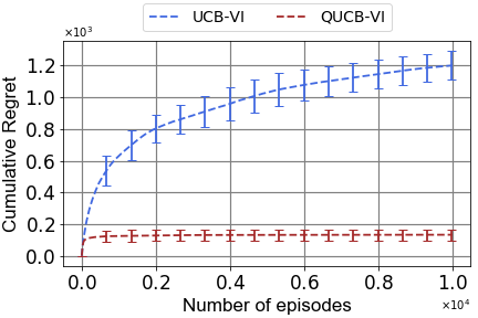
(a) Riverswim-6. $S=6,~{}A=2.$

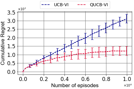
(b) Riverswim-12. $S=12,~{}A=2.$

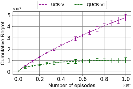
(c) Grid-world. $S=20,~{}A=4.$

Figure 2: Cumulative Regret incurred by QUCB-VI (algorithm 1) and UCB-VI algorithm for various RL environments.

By setting, $\delta=1/KH$, we obtain:

$$\mathbb{E} \Big{[}\sum_{k=0}^{K-1}V^{*}(s_{0})-V^{\pi^{k}}(s_{0})\Big{]}$$

$$\leq 2H^{2}S^{2}A\log^{2}(SAH^{2}K^{2})+2,$$ (51)

$$=O(H^{2}S^{2}A\log^{2}(SAH^{2}K^{2})).$$ (52)

This completes the proof of the theorem.

The choice of improved reward bonus term manifests itself in Eq. (44)-(46) and plays a significant role towards QUCB-VI’s overall regret improvement. Further, we note that the Martingale style proof approach and the corresponding Azuma Hoeffding’s inequality, which are typical in the regret bound proof of classical UCB-VI, are not used in the analysis of QUCB-VI algorithm.

6 Numerical Evaluations

In this section, we analyze the performance of QUCB-VI (Algorithm 1) via proof-of-concept experiments on multiple RL environments. Furthermore, we investigate the viability of our methodology against its classical counterpart UCB-VI (Azar et al., 2017; Agarwal et al., 2019). To this end, we first conduct our empirical evaluations on RiverSwim-6 environment comprising of 6 states and 2 actions, which is an extensively used environment for benchmarking model-based RL frameworks (Osband et al., 2013; Tossou et al., 2019; Chowdhury and Zhou, 2022). Next, we extend our testing setup to include Riverswim-12 with 12 states and 2 actions. Finally, we construct a Grid-world environment (Sutton and Barto, 2018) comprising of a $7\times 7$ sized grid and characterized by 20 states and 4 actions.

Simulation Configurations:  In our experiments, for all the aforementioned environments, we conduct training across $K=10^{4}$ episodes, and every episode consists of $H=20$ time-steps. The environment is reset to a fixed initial state at the beginning of each episode. Furthermore, we perform 20 independent Monte-Carlo simulations and collect episode-wise cumulative regret incurred by QUCB-VI, and baseline UCB-VI algorithms. In our implementation of QUCB-VI, we accumulate the estimates of state transition probability model based on uniform sample from the actual transition probability within a window governed by the quantum mean estimation error.

Interpretation of Results  In Figure 2, we report our experimental results in terms of cumulative regret of agents rewards incurred against number of training episodes for each RL environment. In Fig. 2(a)- 2(c), we note that QUCB-VI significantly outperforms classical UCB-VI with a noticeable margin, while QUCB-VI also achieves model convergence within the chosen number of training episodes. These observations support the performance gains in terms of convergence speed of the proposed algorithm as revealed in our theoretical analysis of regret. In Fig. 2(b)-2(c), we observe that classical UCB-VI suffers an increasingly linear trend in regret growth. This indicates that in environments such as RiverSwim-12, Grid-world which are characterized by large diameter MDPs, it is necessary to increase training episodes in order to ensure sufficient exploration by the RL agent with classical environment. This demonstrates that quantum computing helps in significantly faster convergence.

7 Conclusion and Future Work

We propose a Quantum information assisted model-based RL methodology that facilitates an agent’s learning in an unknown MDP environment. To this end, we first present a carefully engineered architecture modeling agent’s interaction with the environment at every time step. Consequently, we outline QUCB-VI Algorithm that suitably incorporates an efficient quantum mean estimator, leading to exponential theoretical convergence speed improvements in contrast to classical UCB-VI proposed in (Azar et al., 2017). Finally, we report evaluations on a set of benchmark RL environment which support the efficacy of QUCB-VI algorithm. As a future work, it will be worth exploring whether the benefits can be translated to model-free as well as continual RL settings.

References

- Agarwal et al. (2019) Alekh Agarwal, Nan Jiang, Sham M Kakade, and Wen Sun. Reinforcement learning: Theory and algorithms. CS Dept., UW Seattle, Seattle, WA, USA, Tech. Rep, pages 10–4, 2019.
- Aïmeur et al. (2013) Esma Aïmeur, Gilles Brassard, and Sébastien Gambs. Quantum speed-up for unsupervised learning. Machine Learning, 90:261–287, 2013.
- Al-Abbasi et al. (2019) Abubakr O Al-Abbasi, Arnob Ghosh, and Vaneet Aggarwal. Deeppool: Distributed model-free algorithm for ride-sharing using deep reinforcement learning. IEEE Transactions on Intelligent Transportation Systems, 20(12):4714–4727, 2019.
- Arunachalam and de Wolf (2017) Srinivasan Arunachalam and Ronald de Wolf. Guest column: A survey of quantum learning theory. ACM Sigact News, 48(2):41–67, 2017.
- Auer et al. (2008) Peter Auer, Thomas Jaksch, and Ronald Ortner. Near-optimal regret bounds for reinforcement learning. Advances in neural information processing systems, 21, 2008.
- Azar et al. (2017) Mohammad Gheshlaghi Azar, Ian Osband, and Rémi Munos. Minimax regret bounds for reinforcement learning. In International Conference on Machine Learning, pages 263–272. PMLR, 2017.
- Brassard et al. (2002) Gilles Brassard, Peter Hoyer, Michele Mosca, and Alain Tapp. Quantum amplitude amplification and estimation. Contemporary Mathematics, 305:53–74, 2002.
- Brassard et al. (2011) Gilles Brassard, Frederic Dupuis, Sebastien Gambs, and Alain Tapp. An optimal quantum algorithm to approximate the mean and its application for approximating the median of a set of points over an arbitrary distance. arXiv preprint arXiv:1106.4267, 2011.
- Cai et al. (2020) Qi Cai, Zhuoran Yang, Chi Jin, and Zhaoran Wang. Provably efficient exploration in policy optimization. In International Conference on Machine Learning, pages 1283–1294. PMLR, 2020.
- Casalé et al. (2020) Balthazar Casalé, Giuseppe Di Molfetta, Hachem Kadri, and Liva Ralaivola. Quantum bandits. Quantum Machine Intelligence, 2:1–7, 2020.
- Chowdhury and Zhou (2022) Sayak Ray Chowdhury and Xingyu Zhou. Differentially private regret minimization in episodic markov decision processes. In Proceedings of the AAAI Conference on Artificial Intelligence, volume 36, pages 6375–6383, 2022.
- Dann et al. (2017) Christoph Dann, Tor Lattimore, and Emma Brunskill. Unifying pac and regret: Uniform pac bounds for episodic reinforcement learning. Advances in Neural Information Processing Systems, 30, 2017.
- Dong et al. (2008) Daoyi Dong, Chunlin Chen, Hanxiong Li, and Tzyh-Jong Tarn. Quantum reinforcement learning. IEEE Transactions on Systems, Man, and Cybernetics, Part B (Cybernetics), 38(5):1207–1220, 2008.
- Du et al. (2019) Simon S Du, Yuping Luo, Ruosong Wang, and Hanrui Zhang. Provably efficient q-learning with function approximation via distribution shift error checking oracle. Advances in Neural Information Processing Systems, 32, 2019.
- Dunjko et al. (2016) Vedran Dunjko, Jacob M Taylor, and Hans J Briegel. Quantum-enhanced machine learning. Physical review letters, 117(13):130501, 2016.
- Dunjko et al. (2017) Vedran Dunjko, Jacob M Taylor, and Hans J Briegel. Advances in quantum reinforcement learning. In 2017 IEEE International Conference on Systems, Man, and Cybernetics (SMC), pages 282–287. IEEE, 2017.
- Grover (1998) Lov K Grover. A framework for fast quantum mechanical algorithms. In Proceedings of the thirtieth annual ACM symposium on Theory of computing, pages 53–62, 1998.
- Hamoudi (2021) Yassine Hamoudi. Quantum sub-gaussian mean estimator. arXiv preprint arXiv:2108.12172, 2021.
- Jerbi et al. (2021) Sofiene Jerbi, Lea M Trenkwalder, Hendrik Poulsen Nautrup, Hans J Briegel, and Vedran Dunjko. Quantum enhancements for deep reinforcement learning in large spaces. PRX Quantum, 2(1):010328, 2021.
- Jin et al. (2018) Chi Jin, Zeyuan Allen-Zhu, Sebastien Bubeck, and Michael I Jordan. Is q-learning provably efficient? Advances in neural information processing systems, 31, 2018.
- Jin et al. (2020) Chi Jin, Zhuoran Yang, Zhaoran Wang, and Michael I Jordan. Provably efficient reinforcement learning with linear function approximation. In Conference on Learning Theory, pages 2137–2143. PMLR, 2020.
- Kearns and Singh (2002) Michael Kearns and Satinder Singh. Near-optimal reinforcement learning in polynomial time. Machine learning, 49:209–232, 2002.
- Lai et al. (1985) Tze Leung Lai, Herbert Robbins, et al. Asymptotically efficient adaptive allocation rules. Advances in applied mathematics, 6(1):4–22, 1985.
- Lumbreras et al. (2022) Josep Lumbreras, Erkka Haapasalo, and Marco Tomamichel. Multi-armed quantum bandits: Exploration versus exploitation when learning properties of quantum states. Quantum, 6:749, 2022.
- Mnih et al. (2016) Volodymyr Mnih, Adria Puigdomenech Badia, Mehdi Mirza, Alex Graves, Timothy Lillicrap, Tim Harley, David Silver, and Koray Kavukcuoglu. Asynchronous methods for deep reinforcement learning. In International conference on machine learning, pages 1928–1937. PMLR, 2016.
- Montanaro (2015) Ashley Montanaro. Quantum speedup of monte carlo methods. Proceedings of the Royal Society A: Mathematical, Physical and Engineering Sciences, 471(2181):20150301, 2015.
- Osband et al. (2013) Ian Osband, Daniel Russo, and Benjamin Van Roy. (more) efficient reinforcement learning via posterior sampling. Advances in Neural Information Processing Systems, 26, 2013.
- Osband et al. (2016) Ian Osband, Benjamin Van Roy, and Zheng Wen. Generalization and exploration via randomized value functions. In International Conference on Machine Learning, pages 2377–2386. PMLR, 2016.
- Paparo et al. (2014) Giuseppe Davide Paparo, Vedran Dunjko, Adi Makmal, Miguel Angel Martin-Delgado, and Hans J Briegel. Quantum speedup for active learning agents. Physical Review X, 4(3):031002, 2014.
- Rebentrost et al. (2014) Patrick Rebentrost, Masoud Mohseni, and Seth Lloyd. Quantum support vector machine for big data classification. Physical review letters, 113(13):130503, 2014.
- Rohde et al. (2018) David Rohde, Stephen Bonner, Travis Dunlop, Flavian Vasile, and Alexandros Karatzoglou. Recogym: A reinforcement learning environment for the problem of product recommendation in online advertising. arXiv preprint arXiv:1808.00720, 2018.
- Saggio et al. (2021) Valeria Saggio, Beate E Asenbeck, Arne Hamann, Teodor Strömberg, Peter Schiansky, Vedran Dunjko, Nicolai Friis, Nicholas C Harris, Michael Hochberg, Dirk Englund, et al. Experimental quantum speed-up in reinforcement learning agents. Nature, 591(7849):229–233, 2021.
- Silver et al. (2017) David Silver, Julian Schrittwieser, Karen Simonyan, Ioannis Antonoglou, Aja Huang, Arthur Guez, Thomas Hubert, Lucas Baker, Matthew Lai, Adrian Bolton, et al. Mastering the game of go without human knowledge. nature, 550(7676):354–359, 2017.
- Strehl et al. (2006) Alexander L Strehl, Lihong Li, Eric Wiewiora, John Langford, and Michael L Littman. Pac model-free reinforcement learning. In Proceedings of the 23rd international conference on Machine learning, pages 881–888, 2006.
- Sutton and Barto (2018) Richard S Sutton and Andrew G Barto. Reinforcement learning: An introduction. MIT press, 2018.
- Tossou et al. (2019) Aristide Tossou, Debabrota Basu, and Christos Dimitrakakis. Near-optimal optimistic reinforcement learning using empirical bernstein inequalities. arXiv preprint arXiv:1905.12425, 2019.
- Wang et al. (2021a) Daochen Wang, Aarthi Sundaram, Robin Kothari, Ashish Kapoor, and Martin Roetteler. Quantum algorithms for reinforcement learning with a generative model. In International Conference on Machine Learning, pages 10916–10926. PMLR, 2021a.
- Wang et al. (2021b) Daochen Wang, Xuchen You, Tongyang Li, and Andrew M Childs. Quantum exploration algorithms for multi-armed bandits. In Proceedings of the AAAI Conference on Artificial Intelligence, volume 35, pages 10102–10110, 2021b.