Robust expected improvement for Bayesian optimization

Abstract

Bayesian Optimization (BO) links Gaussian Process (GP) surrogates with sequential design toward optimizing expensive-to-evaluate black-box functions. Example design heuristics, or so-called acquisition functions, like expected improvement (EI), balance exploration and exploitation to furnish global solutions under stringent evaluation budgets. However, they fall short when solving for robust optima, meaning a preference for solutions in a wider domain of attraction. Robust solutions are useful when inputs are imprecisely specified, or where a series of solutions is desired. A common mathematical programming technique in such settings involves an adversarial objective, biasing a local solver away from “sharp” troughs. Here we propose a surrogate modeling and active learning technique called robust expected improvement (REI) that ports adversarial methodology into the BO/GP framework. After describing the methods, we illustrate and draw comparisons to several competitors on benchmark synthetic exercises and real problems of varying complexity.

Keywords: Robust Optimization; Gaussian Process; Active Learning; Sequential Design

1 Introduction

Globally optimizing a black-box function $f$, finding

$$x^{*}=\operatorname*{\arg\!\min}_{x\in\mathcal{[}0,1]^{d}}\ f(x),$$ (1)

is a common problem in recommender systems (Vanchinathan et al.,, 2014), hyperparameter tuning (Snoek et al.,, 2012b), inventory management (Hong and Nelson,, 2006), and engineering (Randall et al.,, 1981). Here we explore a robot pushing problem (Kaelbling and Lozano-Perez,, 2017). In such settings, $f$ is an expensive to evaluate computer simulation, so one must carefully design an experiment to effectively learn the function (Sacks et al.,, 1989) and isolate its local or global minima. Optimization via modeling and design has a rich history in statistics (Box and Draper,, 2007; Myers et al.,, 2016). Its modern instantiation is known as Bayesian optimization (BO; Mockus et al.,, 1978).

In BO, one fits a flexible response surface to a limited campaign of example runs, obtaining a so-called surrogate $\hat{f}$ (Gramacy,, 2020). Based on that fit – and in particular its predictive equations for new locations $x$ – one then devises a criteria, a so-called acquisition function (Shahriari et al.,, 2016), targeting desirable qualities, such as $x^{\star}$ that minimize $f$. One must choose a surrogate family for $f$, pair it with a fitting scheme for $\hat{f}$, and choose a criteria to solve for acquisitions. BO is an example of active learning (AL) where one attempts to create a virtuous cycle of learning and data collection. Many good solutions exist in this context, and we shall not provide an in-depth review here.

Perhaps the most common surrogate for BO is the Gaussian Process (GP; Sacks et al.,, 1989). For a modern review, see Rasmussen and Williams, (2006) or Gramacy, (2020). The most popular acquisition function is expected improvement (EI; Jones et al.,, 1998). EI balances exploration and exploitation by suggesting locations with either high variance or low mean, or both. Greater detail is provided in Section 3.2. EI is highly effective and has desirable theoretical properties.

Figure 1: Surface for a 1d multimodal function shown with different adversary levels and $\alpha$-neighborhoods.

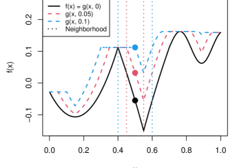
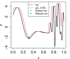
Our goal in this paper is to extend BO via GPs and EI to a richer, more challenging class of optimization problems. In situations where there are a multitude of competing, roughly equivalent local solutions to Eq. (1) a practitioner may naturally express a preference for ones which enjoy a wider domain of attraction; i.e., those whose troughs are larger. Such preferences for robust solutions are expressed across diverse disciplines, e.g., aerospace engineering (Li et al.,, 2002), electrical engineering (Kolvenbach et al.,, 2018), economics (Goldfarb and Iyengar,, 2003). Later we demonstrate a real world autonomous warehousing problem (Kaelbling and Lozano-Perez,, 2017) that benefits from robust design. For a simple example, consider $f(x)$ defined in Eq. (11), provided later in Section 4.2, as characterized by the black line in Figure 1. It has three local minima. The one around $x=0.9$ is significantly higher than the other two; the one around 0.55 is quite narrow but has a lower objective value compared to the local minimum around 0.15. However, that solution is more robust because it has it has a wider area of low-values nearby. Although BO via GPs/EI would likely explore both domains of attraction to a certain extent eventually, it will in the near term (i.e., for smaller simulation budgets) focus on the deeper/narrower one, providing lower resolution on the solution than many practitioners prefer.

Finding or exploring the robust global solution space requires a modification to both the problem and the BO strategy. Here we borrow a framework first introduced in the math programming literature on robust optimization (e.g., Menickelly and Wild,, 2020): an adversary. Adversarial reasoning is popular in reinforcement learning (Huang et al.,, 2011). To our knowledge, the mathematical programming notion of an adversary has never been deployed for BO, where it is perhaps best intuited as a penalty on “sharp” local minima. Specifically, let $x^{\alpha}$ denote the $\alpha$-neighborhood of an input $x$. There are many ways to make this precise depending on context. If $x$ is one-dimensional, then $x^{\alpha}=[x-\alpha,x+\alpha]\equiv[x\pm\alpha]$ is sensible. In higher dimension, one can generalize to an $\alpha$-ball or hyper-rectangle. More specifics will come later. Relative to that $\alpha$-neighborhood, an adversary $g(x,\alpha)$ and robust minimum $x^{r}$ may be defined as follows:

$$\mbox{Let}\quad g(x,\alpha)=\max_{x\in x^{\alpha}}\ f(x)\quad\quad\mbox{so that}\quad\quad x^{r}=\operatorname*{\arg\!\min}_{x\in[0,1]^{d}}\ g(x,\alpha).$$ (2)

Figure 1 provides some examples. Observe that the larger $\alpha$ is, the more “flattened” $g(x,\alpha)$ is compared to $f(x)$. In particular, note how the penalization is more severe in the sharper minimum compared to the shallow trough which is only slightly higher than the original, unpenalized function.

The conventional, local, approach to finding the robust solution $x^{r}$ is best understood as an embellishment of schemes inspired by Newton’s method (e.g., Cheney and Goldstein,, 1959). First, extract derivative (and adversarial) information nearby through finite differencing and evaluation at the boundary of $x^{\alpha}$; then take small steps that descend the (adversarial) surface. Such schemes offer tidy local convergence guarantees but are profligate with evaluations. Leyffer et al., (2020) provide a survey of many of such methods, e.g., AIMSS (Bisschop and Entriken,, 1993), JuMPeR (Dunning et al.,, 2017), ROC (Bertsimas et al.,, 2019; Vayanos et al.,, 2022), ROME (Goh and Sim,, 2009), ROPI (Goerigk,, 2014), SIPAMPL (Vaz and Fernandes,, 2006), and YAMIP (Löfberg,, 2008). When $f$ is expensive, these approaches are infeasible. We believe that idea of building an adversary can be ported to the BO framework, making better use of limited simulation resources toward global optimization while still favoring wider domains of attraction.

The crux of our idea is as follows. A GP $\hat{f}_{n}$, that would typically be fit to a collection of $n$ evaluations of $f$ in a BO framework, can be used to define the adversarial realization of those same values following the fitted analog of $g$: $\hat{g}(x_{i},\alpha)=\max_{x\in x_{i}^{\alpha}}\hat{f}(x)$. A second GP, $\hat{f}^{\alpha}_{n}$, can be fit to those $\hat{g}(x_{i},\alpha)$-values, $i=1,\dots,N$. We call $\hat{f}^{\alpha}_{n}$ the adversarial surrogate. Then, one can use $\hat{f}^{\alpha}_{n}$ as you would an ordinary surrogate, $\hat{f}_{n}$, with EI guiding acquisitions. We call this robust expected improvement (REI). There are, of course, myriad details and variations – simplifications and embellishments – that we are glossing over here, and that we shall be more precise about in due course. The most interesting of these may be how we suggest dealing with a practitioner’s natural reluctance to commit to a particular choice of $\alpha$, a priori.

Before discussing details, it is worth remarking that the term “robust” has many definitions across the statistical and optimization literature(s). Our use of this term here is more similar to some than others. We do not mean robust to outliers (Martinez-Cantin et al.,, 2009) as may arise when noisy, leptokurtic simulators $f$ are involved (Beland and Nair,, 2017) – though we shall have some thoughts on this setup later. Nor do we mean robust to uncontrollable input variables, as in robust parameter design (Taguchi,, 1986), although again there are similarities. Some refer to robustness as the choice of random initialization of a local optimizer (Taddy et al.,, 2009). However our emphasis is global. Our definition in Eq. (2), and its BO implementation, bears some similarity to Oliveira et al., (2019) and to so-called “unscented BO” (Nogueira et al.,, 2016), where robustness over noisy or imprecisely specified inputs is considered. However, our adversary entertains a worst-case scenario (e.g., Bogunovic et al.,, 2018), rather than the stochastic/expected-case. Marzat et al., (2016) also consider worst-case robustness, but focus on so-called “minimax” problems where some dimensions are perfectly controlled ($\alpha=0$) and others are completely uncontrolled ($\alpha=1$). Our definition of robustness – $x^{r}$ in Eq. (2) – emphasizes a worst-case within the $\alpha$-neighborhood, $x^{\alpha}$. When data are scaled, $\alpha$ can be thought of as a percentage; you want to find the best, worst-case scenario when you can control your inputs within $\alpha\times 100\%$. Nonetheless, these other methods and their test cases make for interesting empirical comparisons, as we demonstrate.

The rest of this paper continues as follows. Section 2 reviews the bare essentials required to understand our idea. Section 3 introduces our proposed robust BO setup, via adversaries, surrogate modeling and REI, and variations. Section 4 showcases empirical results via comparison to REI and to similar methodology from the recent BO literature. Section 5 then ports that benchmarking framework to a real world robot pushing problem. Finally, Section 6 concludes with a brief discussion.

2 Review

Here we review the basic elements of BO: GPs and EI.

2.1 Gaussian process regression

A GP may be used to model smooth relationships between inputs and outputs for expensive black-box simulations as follows. Let $x_{i}\in[0,1]^{d}$ represent $d$-dimensional inputs and $y_{i}=f(x_{i})$ be outputs, $i=1,\dots,n$. We presume $y_{i}$ are deterministic realizations of $f$ at $x_{i}$, though the GP/BO framework may easily be extended to noisy outputs (see, e.g., Gramacy,, 2020, Section 5.2.2 and 7.2.4). Collect inputs into $X_{n}$, an $n\times d$ matrix with rows $x_{i}^{\top}$, and outputs into column $n$-vector $Y_{n}$. These are the training data, $D_{n}=(X_{n},Y_{n})$. Then, model $Y_{n}\sim\mathcal{N}_{n}(\mu(X_{n}),\Sigma(X_{n},X_{n}))$, i.e., presume outputs follow an $n$-dimensional multivariate normal distribution (MVN). Since our outputs $y_{i}$ are deterministic, the Gaussian distribution is not on the responses – even though it is notated that way for compactness – but actually on on the latent (random) field of function realizations, $f$.

Often, $\mu(X_{n})=0$ is sufficient for coded inputs and outputs (i.e., after centering and normalization), moving all of the modeling “action” into the covariance structure $\Sigma(\cdot,\cdot)$, which is defined through the choice of a positive-definite, distance-based kernel. Here, we prefer a squared exponential kernel, but others such as the Matèrn (Stein,, 1999; Abrahamsen,, 1997) are common. This choice is not material to our presentation; both specify that the function $f$, via $x_{i}$ and $y_{i}$, vary smoothly as a function of inverse distance in the input space. Details can be found in Gramacy, (2020, Section 5.3.3). Specifically, we fill the covariance structure $\Sigma_{ij}\equiv\Sigma(X_{n},X_{n})_{ij}$ via

$$\Sigma_{ij}=\tau^{2}\left(\textrm{exp}\left(-\frac{||x_{i}-x_{j}||^{2}}{\theta}\right)+\epsilon\mathbb{I}_{\{i=j\}}\right).$$ (3)

The structure in Eq. (3) is hyperparameterized by $\tau^{2}$ and $\theta$. Let $\hat{\tau}^{2}$ and $\hat{\theta}$ be estimates for the hyperparameters estimated through the MVN log likelihood. Scale $\tau^{2}$ captures vertical spread between peaks and valleys of $f$. Lengthscale $\theta$ captures how quickly the function changes direction. Larger $\theta$ means the correlation decays less quickly leading to flatter functions. Observe that $\epsilon$-jitter (Neal,, 1998) is added to the diagonal to ensure numerical stability when decomposing $\Sigma$.

Working with MVNs lends a degree of analytic tractability to many statistical operations, in particular for conditioning (e.g., Kalpić and Hlupić,, 2011) as required for prediction. Let $\mathcal{X}$, an $n_{p}\times d$ matrix, store inputs for “testing.” Then, the conditional distribution for $Y(\mathcal{X})$ given $D_{n}=(X_{n},Y_{n})$ is also MVN and has a convenient closed form:

$$Y(\mathcal{X})\mid D_{n}\sim\mathcal{N}_{n_{p}}(\mu_{n}(\mathcal{X}),\Sigma_{n}(\mathcal{X}))$$ (4)

where $$\mu_{n}(\mathcal{X})=\Sigma(\mathcal{X},X_{n})\Sigma^{-1}(X_{n},X_{n})Y_{n}$$

and $$\Sigma_{n}(\mathcal{X})=\Sigma(\mathcal{X},\mathcal{X})-\Sigma(\mathcal{X},X_{n})\Sigma^{-1}(X_{n},X_{n})\Sigma(X_{n},\mathcal{X}),$$

where $\Sigma(\cdot,\cdot)$ extends $\Sigma_{ij}\equiv\Sigma(x_{i},x_{j})$ in Eq. (3) to the rows of $\mathcal{X}$ and between $\mathcal{X}$ and $X_{n}$. The diagonal of the $n_{p}\times n_{p}$ matrix $\Sigma_{n}(\mathcal{X})$ provides pointwise predictive variances which may be denoted as $\sigma_{n}^{2}(\mathcal{X})$. Later, we shall use $\text{GP}_{\hat{\theta}}(D_{n})$ to indicate a GP surrogate $\hat{f}_{n}$ fitted to data $D_{n}=(X_{n},Y_{n})$ emitting predictive equations $(\mu_{n}(\cdot),\sigma_{n}^{2}(\cdot))$ as in Eq. (4), conditioned on estimated hyperparameters $\hat{\theta}_{n}$. Note that we are streamlining the notation here somewhat and subsuming $\hat{\tau}^{2}$ into $\hat{\theta}$. For more information on GPs, see Gramacy, (2020, Chapter 5) or Santner et al., (2018).

2.2 Expected improvement

Bayesian Optimization (BO) seeks a global minimum (1) under a limited experimental budget of $N$ runs. The idea is to proceed sequentially, $n=n_{0},\dots,N$, and in each iteration $n$ make a greedy selection of the next, $n+1^{\mathrm{st}}$ run, $x_{n+1}$, based on solving an acquisition function tied to $\hat{f}_{n}$. The initial $n_{0}$-sized design could be space-filling, for example with a Latin hypercube sample (LHS) or maximin design (Dean et al.,, 2015, Chapter 17) or, as some have argued (Zhang et al.,, 2020), purely at random. GPs have emerged as the canonical surrogate for BO. Although there are many acquisition functions in the literature tailored to BO via GPs, expected improvement (EI) is perhaps the most popular. EI may be described as follows.

Let $f^{\min}_{n}=\min(y_{1},\dots,y_{n})$ denote the best “best observed value” (BOV) found so far, after the first $n$ acquisitions ($n_{0}$ of which are space-filling/random). Then, define the improvement at input location $x$ as $I(x)=\max\{0,f^{\min}_{n}-Y(x)\}$. $I(x)$ is a random variable, inheriting its distribution from $Y(x)\mid D_{n}$. If $Y(x)$ is Gaussian, as it is under $\text{GP}_{\hat{\theta}}(D_{n})$ via Eq. (4), then the expectation of $I(x)$ has a closed form:

$$\mathrm{EI}_{n}(x)=\mathbb{E}\{I(x)|D_{n}\}=(f^{\min}_{n}-\mu_{n}(x))\Phi\left(\frac{f_{n}^{\min}-\mu_{n}(x)}{\sigma_{n}(x)}\right)+\sigma_{n}(x)\phi\left(\frac{f_{n}^{\min}-\mu_{n}(x)}{\sigma_{n}(x)}\right),$$ (5)

where $\Phi$ and $\phi$ are the standard Gaussian CDF and PDF, respectively. Notice how EI is a weighted combination of mean $\mu_{n}(x)$ and uncertainty $\sigma_{n}(x)$, trading off “exploitation and exploration.” The first term of the sum is high when $\hat{f}(x)$ is much lower than $f_{n}^{\min}$, while the second term is high when the GP has high uncertainty at $x$.

Figure 2: Left: EI-based (EGO) acquisition with $n_{0}=10$ initial points as black squares and 10 acquisitions as blue circles using EGO on the 1D example function from Eq. (11) with initial GP fit in blue. Right: EI using the initial design at different locations of $x$.

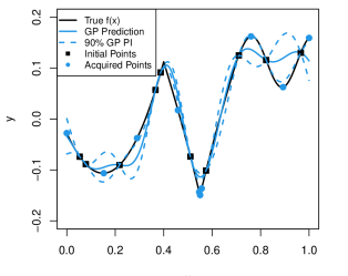
The right panel of Figure 2 shows an EI surface implied by the GP surrogate (blue) shown in the left panel. This fit is derived from $n=10$ training data points (black squares) sampled from our $f(x)$ from Figure 1. We will discuss the blue circles momentarily. Observe how EI is high in the two local troughs of minima, near $x=0.15$ and $x=0.55$, but away from the training data. The total volume (area under the curve) of EI is larger around the left, shallower trough, but the maximal EI location is in the right, spiky trough. This ($x$ near 0.55) is where EI recommends choosing the next, $n+1^{\mathrm{st}}$ acquisition.

Operationalizing that process, i.e., numerically solving for the next acquisition involves its own, “inner” optimization: $x_{n+1}=\operatorname*{\arg\!\max}_{x\in[0,1]^{d}}\;\mathrm{EI}_{n}(x)$. This can be challenging because EI is multi-modal. Observe that while $f$ only has two local minima, EI as shown for $n=10$ in Figure 2, has three local maxima. So in some sense the inner optimization is harder than the “outer” one. As $n$ grows, the number of local EI maxima can grow. A numerical optimizer such as BFGS (Byrd et al.,, 1995) is easily stuck, necessitating a multi-start scheme (Burden and Faires,, 1989). Another common approach is to use a discrete, space-filling set of candidates, turning a continuous search for $x\in[0,1]^{d}$ into a discrete one for $x\in\mathcal{X}_{\mathrm{cand}}$. Hybrid and smart-candidate schemes are also popular (Scott et al.,, 2011; Gramacy et al.,, 2022). In general, we can afford a comprehensive effort toward solving the “inner” optimization because the objective, derived from $\text{GP}_{\hat{\theta}}(D_{n})$, is cheap – especially compared to the black-box $f(\cdot)$. Repeated application of EI toward selecting $x_{n+1}$ is known as the efficient global optimization algorithm (EGO, Jones et al.,, 1998).

The blue circles in Figure 2 indicate how nine further acquisitions (ten total) play out, i.e., $10=n_{0},\dots,n,\dots,N=20$ in EGO. Notice that the resulting training data set $D_{N}$, combining both black and blue points concentrates acquisitions in the “tip” of the spiky, right trough. The rest of the space, including the shallower left trough, is more uniformly (and sparsely) sampled. Our goal is to concentrate more acquisition effort in the shallower trough.

3 Proposed methodology

Here we extend the EGO algorithm by incorporating adversarial thinking. The goal is to find $x^{r}$ from Eq. (2) for some $\alpha$. We begin by presuming a fixed, known $\alpha$ selected by a practitioner.

3.1 The adversarial surrogate

If $\hat{f}_{n}(x)$ is a surrogate for $f(x)$, then one may analogously notate $\hat{f}_{n}^{\alpha}(x)$ as a surrogate for $g(x,\alpha)$, an adversarial surrogate. We envision several ways in which $\hat{f}_{n}^{\alpha}(x)$ could be defined in terms of $\hat{f}_{n}(x)$, but not many which are tractable to work with analytically or numerically. For example, suppose $Y^{\alpha}(x)=\max_{x^{\prime}\in x^{\alpha}}Y(x^{\prime})$, where $Y(x^{\prime})\sim\mathcal{N}(\mu_{n}(x^{\prime}),\sigma^{2}_{n}(x^{\prime}))$, a random variable whose distribution follows the spirit of Eq. (2), but uses the predictive equations of Eq. (4). The distribution of $Y^{\alpha}(x)$ could be a version of $\hat{f}_{n}^{\alpha}(x)$, at least notionally. However a closed form remains elusive.

Instead, it is rather easier to define $\hat{f}_{n}^{\alpha}(x)$ as an ordinary surrogate trained on data derived through adversarial reasoning on the original surrogate $\hat{f}_{n}(x)$. Let $Y_{n}^{\alpha}$ denote these adversarial responses, where each $y_{i}^{\alpha}$, for $i=1,\dots,n$, follows

$$y_{i}^{\alpha}=\max_{x\in x^{\alpha}_{i}}\;\mu_{n}(x)\quad\mbox{where $x_{i}^{\alpha}$ is the $\alpha$-neighborhood of the $i^{\mathrm{th}}$ entry of $X_{n}$, as usual.}$$ (6)

There are many sensible choices for finding $y_{i}^{\alpha}$ numerically. Newton-based optimizers, e.g., BFGS, could leverage closed form derivatives for $\mu_{n}(x)$ finite differencing. A simpler option that works well is to instead take $y_{i}^{\alpha}=\max_{x\in x_{i}^{\mathcal{B}_{\alpha}(x)}}\mu_{n}(x)$, where $\mathcal{B}_{\alpha}(x)$ is the discrete set of points on the corners of a box with sides of length $\alpha$ emanating from $x$. Details for our own implementation are deferred to Section 4.1.

Given $Y_{n}^{\alpha}$, an adversarial surrogate may be built by modeling adversarial data $D_{n}^{\alpha}=(X_{n},Y_{n}^{\alpha})$, i.e., $Y_{n}^{\alpha}$ paired with their original inputs, as a GP. Let $\hat{\theta}_{\alpha}$ denote hyperparameter estimates for $\hat{f}_{n}^{\alpha}(x)$. Fill in the covariance matrix following Eq. (3), $\Sigma^{\alpha}(\cdot,\cdot)$. Finally, define the adversarial surrogate as

$$\hat{f}_{n}^{\alpha}(x)\equiv\text{GP}_{\hat{\theta}_{\alpha}}(D_{n}^{\alpha})\rightarrow(\mu_{n}^{\alpha}(\cdot),\sigma_{n}^{2\alpha}(\cdot))$$ (7)

via novel hyperparameter estimates $\hat{\theta}_{\alpha}$ using $Y_{n}^{\alpha}$ rather than $Y_{n}$ with predictive equations akin to (4). Since the $Y_{n}^{\alpha}$ are the original surrogate’s ($\hat{f}_{n}$) estimate of adversarial response values according $f_{\alpha}$, $\hat{f}_{n}^{\alpha}$ may serve as a surrogate for $g(x,\alpha)$ from the left half of Eq. (2).

Figure 3: Left: The same black and blue lines from Figure 2. In red, $Y_{n}^{\alpha}$ are shown as the points with $\hat{f}_{n}^{\alpha}(x)$ as the curve. Right: Robust expected improvement for the current design.

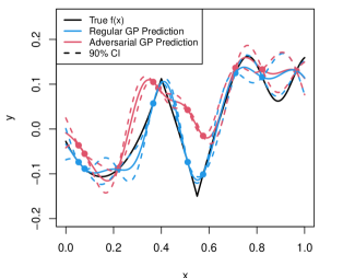
As a valid GP, $\hat{f}_{n}^{\alpha}$ can be used in any way another surrogate might be deployed downstream. For example, $\hat{f}_{n}^{\alpha}$ may be used to acquire new runs via EI, but hold that thought for a moment. To illustrate $\hat{f}_{n}^{\alpha}$, the left panel of Figure 3 augments the analogous panel in Figure 2 to include a visual of $\hat{f}_{n}^{\alpha}$ via $\mu_{n}^{\alpha}$ and error-bars $\mu_{n}^{\alpha}\pm\sigma_{n}^{\alpha}$. Notice that the new, red lines, are much higher near the sharp minimum (near $x=0.5$), but less dramatically elevated for the wider, dull trough near $x=0.2$.

Also observe in Figure 3 that, whereas for the most part $\mu_{n}(x)\leq\mu^{\alpha}_{n}(x)$, this reverses for a small portion of the input domain near $x=0.2$. That would never happen when comparing $f(x)$ to $g(x,\alpha)$ via Eq. (2). This happens for our surrogates – original $\hat{f}_{n}$ and adversarial $\hat{f}_{n}^{\alpha}$ – for two reasons. One is that both are stationary processes because their covariance structure (3) uses only relative distances, resulting in a compromise surface between sharp and dull. Although this is clearly a mismatch to our data-generating mechanism, we have not found any downsides in our empirical work. Possibly improved performance for non-stationary surrogates is entertained in Section 6. The other reason is that the adversarial data $Y_{n}^{\alpha}$, whether via a stationary or (speculatively) a non-stationary surrogate $\hat{f}_{n}$, provide a low-resolution view of the true adversary $g(x,\alpha)$ when $n$ is small. Consequently, $\hat{f}_{n}^{\alpha}$ is a crude approximation to $g(x,\alpha)$, but that will improve with more acquisitions (larger $n$). What is most important is the EI surface(s) that the surrogate(s) imply. These are shown in the right panel of Figure 3, and discussed next.

3.2 Robust expected improvement

Robust expected improvement (REI), $\mathrm{EI}_{n}^{\alpha}(\cdot)$, is the analog of in Eq. (5) except using $(\mu_{n}^{\alpha}(\cdot),\sigma_{n}^{2\alpha}(\cdot))$, towards solving the mathematical program given in the right half of Eq. (2). Let $f_{n}^{\alpha,\min}=\min(y_{1}^{\alpha},\dots,y_{n}^{\alpha})$ denote the best estimated adversarial response (BEAR). Then, let

$$\text{EI}^{\alpha}_{n}(x)=\mathbb{E}\{I(x)\mid D_{n}^{\alpha}\}=(f_{n}^{\alpha,\min}-\mu_{n}^{\alpha}(x))\Phi\!\left(\frac{f_{n}^{\alpha,\min}-\mu_{n}^{\alpha}(x)}{\sigma_{n}^{\alpha}(x)}\right)+\sigma_{n}^{\alpha}(x)\phi\!\left(\frac{f_{n}^{\alpha,\min}-\mu_{n}^{\alpha}(x)}{\sigma_{n}^{\alpha}(x)}\right).$$ (8)

The right panel of Figure 3 shows an REI surface arising from the same initial setup as Figure 2. We see only one peak, located at the shallower, wider trough compared to three peaks for EI [Figure 2]. Generally speaking, REI surfaces have fewer local maxima compared to EI because $\hat{f}_{n}^{\alpha}(x)$ smooths over the peaked regions. Thus the inner optimization of REI often has fewer local minima, requiring fewer multi-starts.

REI is summarized succinctly in Eq. (8) above, but it is important to appreciate that it is a result of a multi-step process. Alg. 1 provides the details: fit an ordinary surrogate, which is used to create adversarial data, in turn defining the adversarial surrogate upon which EI is evaluated. The algorithm is specified for a particular reference location $x$, used toward solving $x_{n+1}=\operatorname*{\arg\!\max}_{x\in[0,1]^{d}}\;\text{EI}_{n}^{\alpha}(x)$. It may be applied identically for any $x$. In a numerical solver it may be advantageous to cache quantities unchanged in $x$.

input $D_{n}=(X_{n},Y_{n})$, $x$, and $\alpha$

$\hat{f}_{n}(x)=\text{GP}_{\hat{\theta}}(D_{n})$

  // with predictive moments in Eq. (4)

for i = 1, $\dots$, $n$ do

       $y_{i}^{\alpha}$ = ${\operatorname*{\arg\!\max}_{x^{\prime}\in x^{\alpha}_{i}}}\ \mu_{n}(x^{\prime})$

        // adversarial responses, (6)

      

$D_{n}^{\alpha}=(X_{n},Y_{n}^{\alpha})=(X_{n},\{y_{i}^{\alpha}\}_{i=1}^{n})$

$\hat{f}^{\alpha}_{n}(x)=\text{GP}_{\hat{\theta}_{\alpha}}(D_{n}^{\alpha})$

  // the adversarial surrogate, (7)

return $(\text{EI}_{n}^{\alpha}(x))$

  // EI using $\hat{f}^{\alpha}_{n}(x)$ from the previous line, (8)

Algorithm 1 Robust Expected Improvement

With repeated acquisition via EI, over $n=n_{0},\dots,N-1$ being known as EGO, we dub robust efficient global optimization (REGO) as the repeated application of REI towards finding a robust minimum. REGO involves a loop over Alg. 1, with updates $D_{n}\rightarrow D_{n+1}$ after each acquisition. The final data set, $D_{N}=(X_{N},Y_{N})$ provides insight into both $f(x)$ and $g(x,\alpha)$ and their minima. Whereas EGO would report BOV $f_{N}^{\min}$, and/or the corresponding element $x^{\star}_{\mathrm{bov}}$ of $X_{N}$, REGO would report the BEAR $f_{N}^{\alpha,\min}$, the same quantity used to define REI in Eq. (8), and/or input $x^{\star}_{\mathrm{bear}}$.

Post hoc adversarial surrogate

To quantify the advantages of REI/REGO over EI/EGO in our empirical work of Sections 4–5, we consider a post hoc adversarial surrogate. This is the surrogate constructed after running all acquisitions, $n_{0}+1,\dots,N$ via EI/EGO, then at $N$ fitting an adversarial surrogate Eq. (7), and extracting the BEAR $f_{N}^{\alpha,\min}$ rather than the BOV. In other words, the last step is faithful to the adversarial goal, whereas active learning aspects ignore it and proceed as usual. While the BOV from EGO can be a poor approximation to the robust optimum $f(x^{r})$ of Eq. (2), the BEAR from a post hoc adversarial surrogate can potentially be better. Comparing two BEAR solutions, one from REGO and one from a post hoc EGO surrogate, allows us to separately explore the value of REI acquisitions from post hoc adversarial surrogates, $\hat{f}_{N}^{\alpha}$.

Figure 4: Left: Surrogate and post hoc surrogate fits after EGO acquisitions ($N=20$ and $n_{0}=10$) on Eq. (11). Right: Same except REGO where BOV and BEAR are the same.

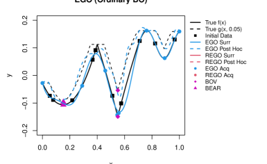
To illustrate on our running example, consider the outcome of EGO, from the left panel of Figure 2, recreated in the Figure 4 (left). In both, the union of black and blue points comprise $D_{N}$. In Figure 4 the dashed blue curve provides the post hoc adversarial surrogate, $\hat{f}_{N}^{\alpha}$, from these runs, with the BOV and BEAR indicated as magenta diamonds and triangles, respectively. Notice that for EGO, the BOV is around the global, peaked minimum, but the BEAR captures the shallow, robust minimum. The analogous REGO run, via EI acquisitions (red circles) and adversarial surrogate (red lines) is shown in the right panel of Figure 4. Here BEAR and BOV estimates are identical since REGO does not explore the peaked minimum.

Looking at both panels of Figure 4, the BEAR offers a robust solution for both EGO or REGO. However, EGO puts only one of its acquisitions in the wide trough compared to four from REGO. Consequently, REGO’s BEAR offers a more accurate estimate for $x^{r}$. With only $N=20$ points in 1d, any sensible acquisition strategy should yield a decent meta-model for $f(x)$ and $g(x,\alpha)$, so we may have reached the limits of the utility of this illustrative example. In Sections 4–5 we intend to provide more compelling evidence that REGO is better at targeting robust minima. Before turning to that empirical study, we introduce two REI variations that feature in some of those examples.

Unknown and vector-valued $\alpha$

Until this point we have presumed fixed, scalar $\alpha$, perhaps specified by a practitioner. In the case of inputs $x$ coded to the unit cube $[0,1]^{d}$, a choice of $\alpha=0.05$, say, represents a robustness specification of 5% in each coordinate direction (totaling 10% of each dimension), i.e., where $x^{\alpha}\equiv[x_{j}\pm\alpha:j=1,\dots,d]$. This intuitive relationship can be helpful in choosing $\alpha$, however one may naturally wish to be “robust” to this specification. Suppose instead we had an $\alpha_{\max}$ in mind, where $0\leq\alpha\leq\alpha_{\max}$. If REI is robust to every value $0\leq\alpha\leq\alpha_{\max}$, then a slight misspecification in $\alpha_{\max}$ is still robust over most of the same $\alpha$ values. Whereas a slight misspecification in pinpointing $\alpha$ may lead to a completely different response. One option that allows us be robust over the range of $0$ to $\alpha_{\max}$ is to simply run REGO with $\alpha\leftarrow\alpha_{\max}$, i.e., basing all REI acquisitions on $\alpha_{\max}$ instead. Although we do not show this to save space, performance (via BEAR) of $\alpha_{\max}$ relative to a nominal $\alpha$ rapidly deteriorates as the gap between $\alpha_{\max}$ and $\alpha$ widens.

A better method is to base REI acquisitions on all $\alpha$-values between zero and $\alpha_{\max}$ by integrating over them: $\overline{\mathrm{EI}}^{\alpha_{\max}}_{n}=\int_{0}^{\alpha_{\max}}\text{EI}^{\alpha}_{n}(x)\;dF(\alpha)$, say over uniform measure $F$. We are not aware of an analytically tractable solution, in part because embedded in $\text{EI}^{\alpha}_{n}(x)$ are complicated processes such as determining adversarial data, and surrogates fit thereupon. But quadrature is relatively straightforward, either via Monte Carlo (MC) $\alpha^{(t)}\sim F$, for $t=1,\dots,T$, over a grid $\{0=\alpha^{(1)},\dots,\alpha^{(T)}=\alpha_{\max}\}$. Define

$$\overline{\mathrm{EI}}^{\alpha_{\max}}_{n}\approx\frac{1}{T}\sum_{t=1}^{T}\text{EI}^{\alpha^{(t)}}_{n}(x)\quad\mbox{ for the former,}\quad\mbox{or}\quad\overline{\mathrm{EI}}^{\alpha_{\max}}_{n}\approx\frac{1}{T}\sum_{t=1}^{T}\text{EI}^{\alpha^{(t)}}_{n}(x)F(\alpha^{(t)}),$$ (9)

for the latter. Both may be implemented by looping over Alg. 1 with different $\alpha^{(t)}$ values, and then averaging to take $x_{n+1}=\operatorname*{\arg\!\max}_{x\in[0,1]^{d}}\overline{\text{EI}}^{\alpha_{\max}}_{n}$. Both approximations improve for larger $T$.

With random $\alpha^{(t)}\sim F$, even a single draw ($T=1$) suffices as an unbiased estimator – though clearly with high variance. This has the advantage of a simpler implementation, and faster execution as no loop over Alg. 1 is required. In our empirical work to follow, we refer to this simpler option as the “rand” approximation, and the others (MC or grid-based) as “sum”. It is remarkable how similarly these options perform, relative to one another and to a nominal REI with a fixed $\alpha$-value. One could impose $\alpha_{\min}>0$ similarly, though we do not entertain this variation here.

As a somewhat orthogonal consideration, it may be desirable to entertain different levels of robustness – different $\alpha$-values $\{\alpha_{1},\dots,\alpha_{d}\}$ – in each of the $d$ coordinate directions. The only change this imparts on the description above is that now $x^{\alpha}=[x_{j}\pm\alpha_{j}:j=1,\dots,d]$, a hyperrectangle rather than hypercube. Other quantities such as $g(x,\alpha)$ and $\text{EI}_{n}^{\alpha}(x)$ remain as defined earlier with the understanding of a vectorized $\alpha=\{\alpha_{1},\dots,\alpha_{d}\}$ under the hood. Using vectorized $\alpha_{\max}$ in Eq. (9) requires draws from a multivariate $F$, which may still be uniform, or a higher dimensional grid of $\alpha^{(t)}$, recognizing that we are now approximating a higher dimensional integral. We note that allowing an $\alpha_{j}$ to span the entire range of the $j^{\mathrm{th}}$ coordinate, while other $\alpha_{k}$ are zero, mimicks a setup similar to robust parameter design (Taguchi,, 1986). However, our BO context is quite different from classical response surface methods (RSMs, e.g., Myers et al.,, 2016). In particular, RSMs involve second-order, local models rather than global surrogates.

4 Implementation and benchmarking

Here we provide a description of our implementation, variations, methods of our main competitors, evaluation metrics and ultimately provide a suite of empirical comparisons.

4.1 Implementation details

Our main methods (REI/REGO, variations and special cases) are coded in R (R Core Team,, 2021). These codes may be found, alongside those of our comparators and all empirical work in this paper, in our public Git repository: https://bitbucket.org/gramacylab/ropt/. GP surrogate modeling for our new methods – our competitors may leverage different subroutines/libraries – is provided by the laGP package (Gramacy,, 2016), on CRAN. Those subroutines, which are primarily implemented in C, leverage squared exponential covariance structure (3), and provide analytic $\hat{\tau}^{2}$ using maximum likelihood estimation conditional on lengthscale $\theta$. In our main suite of experiments, $\theta$ is fixed to appropriate values in order to control MC variation that otherwise arises in repeated MLE-updating of $\hat{\theta}$, especially in small-$n$ cases. In Appendix A we demonstrate how these results change when $\hat{\theta}$ is estimated. More details are provided as we introduce our test cases, with further discussion in Section 6. Throughout we use $\epsilon=10^{-8}$ in Eq. (3), as appropriate for deterministic blackbox objective function evaluations. For ordinary EI calculations we use add-on code provided by Gramacy, (2020, Chapter 7.2.2). All empirical work was conducted on an 8-core hyperthreaded Intel i9-9900K CPU at 3.60 GHz with Intel MKL linear algebra subroutines.

Section 3.1 introduced several possibilities for solving $y_{i}^{\alpha}$, whose definition is provided in Eq. (6). Although numerical optimization, e.g. BFGS, is a gold standard, in most cases we found this to be overkill, resulting in high runtimes for all $(N-N_{0})$ acquisitions with no real improvements in accuracy over the following, far simpler alternative. We prefer quickly optimizing over the discrete set $x^{\mathcal{B}_{\alpha}(x)}$ comprising of a box extending $\alpha$-units out in each coordinate direction from $x$, or its vectorized analog as described in Section 3.2. This “cornering” alternative occasionally yields $y_{i}^{\alpha}<y_{i}$, which is undesirable, but this is easily mitigated by augmenting the box $x^{\mathcal{B}_{\alpha}(x)}$ to contain a small number of intermediate, grid locations in each coordinate direction. Using an odd number of such intermediate points ensures $y_{i}^{\alpha}\geq y_{i}$. For 1d problems, we use three intermediate points and in higher dimension we increase this to five. We find that a $d$-dimensional grid formed from the outer product for each coordinate (i.e., a $2^{5}=32$-point-grid for $d=2$) facilitates a nice compromise between computational thrift, and accuracy of adversarial $y_{i}^{\alpha}$-values compared to the cumbersome BFGS-based alternative.

In our test problems, which are introduced momentarily and utilize inputs coded to $[0,1]^{d}$, we compare each of the three variations of REGO described in Section 3. These comprise: (1) REI with known $\alpha$ (Alg. 1); (2) novel $\alpha\sim\mathrm{Unif}(0,\alpha_{\max})$ at acquisition; and (3) averaging over a sequence of $\alpha\in[0,\alpha_{\max}]$ (9). For all examples, we set $\alpha_{\max}=0.2$ and average over five equally spaced values. In figures, these methods are denoted as “known”, “rand” and “sum”, respectively. After each acquisition, we use the post hoc adversarial surrogate to find the BEAR operating conditions: $x^{*}_{\mathrm{bear}}$ and $f_{N}^{\alpha,\mathrm{min}}$ in order to track progress.

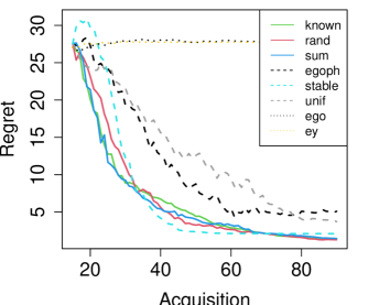
As representatives from the standard BO literature, we compare against the following “straw-men”: EGO (Jones et al.,, 1998), where acquisitions are based on EI (5; and “EY” (Gramacy,, 2020) which works similarly to EGO, except acquisitions are selected minimizing $\mathbb{E}[Y(x)\mid D_{N}]$: $x^{\text{EY}}_{\text{new}}=\operatorname*{\arg\!\min}_{x\in[0,1]^{d}}\mu_{n}(x)$. In other words, EY acquires the point that the surrogate predicts has the lowest mean. Since it does not incorporate uncertainty ($\sigma_{n}(x)$), repeated EY acquisition often stagnates in one region – usually a local minima – rather than exploring new areas like EI does. In our figures, these comparators are indicated, as follows: “ego”, and “ey” respectively for EGO and EY with progress measured by BOV: $x^{*}_{\mathrm{bov}}$ and $f_{N}^{\mathrm{min}}$. Finally, we consider the post hoc adversary with progress measured by BEAR for EGO (“egoph”) and uniform random sampling (“unif”). In the figures, REI methods are solid curves with robust competitors dashed and regular BO dotted.

Our final comparator is StableOPT from Bogunovic et al., (2018). For completeness, we offer the following by way of a high-level overview; details are left to their paper. Bogunovic et al., assume a fixed, known $\alpha$, although we see no reason why our extensions for unknown $\alpha$ could not be adapted to their method as well. Their algorithm relies on confidence bounds to narrow in on $x^{r}$. Let $\mathrm{ucb}_{n}(x)=\mu_{n}(x)+2\sigma_{n}(x)$ denote the upper 95% confidence bound at $x$ for a fitted surrogate $\hat{f}_{n}$, and similarly $\mathrm{lcb}_{n}(x)=\mu_{n}(x)-2\sigma_{n}(x)$ for the analagous lower bound. Then we may translate their algorithm into our notation, shown in Alg. 2, furnishing the $n^{\mathrm{th}}$ acquisition. Similar to REGO, this may then be wrapped in a loop for multiple acquisitions. We could not find any public software for StableOPT, but it was relatively easy to implement in R; see our public Git repo.

input $D_{n-1}=(X_{n-1},Y_{n-1})$ and $\alpha$

$\hat{f}_{n-1}(x)=\mathrm{GP}_{\hat{\theta}}(D_{n-1})$

  // with predictive moments in Eq. (4)

$\tilde{x}_{n}=\operatorname*{\arg\!\min}_{x\in[0,1]^{d}}\max_{a\in[-\alpha,\alpha]}\mathrm{lcb}_{n-1}(x+a)$

  // where we think $x^{r}$ is

$a_{n}=\operatorname*{\arg\!\max}_{a\in[-\alpha,\alpha]}\mathrm{ucb}_{n-1}(\tilde{x}_{n}+a)$

  // worst point within $\tilde{x}_{n}^{\alpha}$

return $(\tilde{x}_{n}+a_{n},f(\tilde{x}_{n}+a_{n})))$

  // sample from $f$ and return

Algorithm 2 StableOPT

Rather than acquiring new runs nearby likely $x^{r}$, StableOPT samples the worst point within $\tilde{x}_{n}^{\alpha}$. Consequently, its final $X_{N}$ does not contain any points thought to be $x^{r}$. Bogunovic et al., recommend selecting $x^{*}_{\mathrm{bear}}$ from all $\tilde{x}_{n}$ rather than the actual points sampled, all $\tilde{x}_{n}+a_{n}$, using notation introduced in Alg. 2. We generally think it is a mistake to report an answer at an untried input location. So in our experiments we calculate $x^{*}_{\mathrm{bear}}$ for StableOPT as derived from a final, post hoc adversary calculation [Section 3.2]. In figures, this comparator is denoted as “stable”.

It is worth noting that there are many additional potential comparators from the math programming community. Some where mentioned in Section 1. Others include ones developed by Menickelly and Wild, (2018); Bertsimas et al., (2010); Conn and Vicente, (2012); Bertsimas and Nohadani, (2010). All involve a test case that is some variation our “Bertsimas” example in Eq. (12), coming momentarily. However, it is clear at a glance that these papers’ results in this case are not competitive against our BEAR benchmark. This is because those methods were developed with different goals in mind. For example, some are inherently local while REI/BO are global. Others require hundreds or thousands of function evaluations to find the true robust minimum. Our budgets shown here are in the dozens. In some cases extensive evaluation makes their methods more precise, but also more profligate with runs. When the goal is to optimize an expensive blackbox function, more evaluation is often impossible and we have to make the most of every acquisition. Finally, none of the robust methods that we found from the math programming literature came with an R implementation. Consequently, we did not include them in our empirical study.

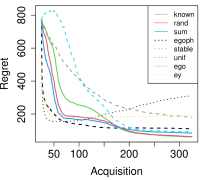
The general flow of our benchmarking exercises coming next [Section 4.2] is as follows. Each optimization, say in input dimension $d$, is seeded with a novel LHS of size $n_{0}=5+5d$ that is shared for each comparator. Acquisitions, $n=n_{0}+1,\dots,N$, separate for each comparator up to a total budget $N$ (different for each problem), are accumulated and progress is tracked along the way. Then this is repeated, for a total of 1,000 MC trials. To simplify notation, let $x^{*}_{\mathrm{b,n}}$ be either $x^{*}_{\mathrm{bear}}$ or $x^{*}_{\mathrm{bov}}$, depending on if using BEAR or BOV, after the $n^{\mathrm{th}}$ acquisition. We utilize the following two metrics to compare BEAR or BOV across methods using the true adversary:

$$r(x^{*}_{\mathrm{b,n}})=g(x^{*}_{\mathrm{b,n}},\alpha)-g(x^{r},\alpha)\quad\quad\quad\quad d(x^{*}_{\mathrm{b,n}})=||x^{*}_{\mathrm{b,n}}-x^{r}||,$$ (10)

where $x^{r}$ is the $x$ location of the true robust minimum. The first metric is similar to the concept of regret from decision theory (Blum and Mansour,, 2007; Kaelbling et al.,, 1996) at the suggested $x^{*}_{\mathrm{b,n}}$. Regret measures how much you lose out by running at $x^{*}_{\mathrm{b,n}}$ compared to $x^{r}$. Regret is always nonnegative since by definition, $x^{r}=\operatorname*{\arg\!\min}_{x\in[0,1]^{d}}g(x,\alpha)$. The second metric is the distance from $x^{*}_{\mathrm{b,n}}$ to $x^{r}$. For both, lower is better with 0 being the floor if a method correctly identifies exactly $x^{r}$ as the BEAR or BOV.

4.2 Empirical comparisons

One-dimensional examples

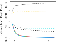
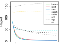
The left panel of Figure 5 shows the 1d RKHS function used by Assael et al., (2014), and an adversary with $\alpha=0.03$.

Figure 5: Left: The RKHS function and the robust surface with $\alpha=0.03$. Middle: $d(x^{*}_{\mathrm{b,n}})$ after each acquisition. Right: $r(x^{*}_{\mathrm{b,n}})$ after each acquisition.

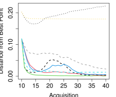
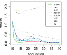
Observe how $f$ has a smooth region for low $x$ values and a wiggly region for high $x$. With $\alpha=0.03$, $x^{r}=0.312$ whereas $x^{*}=0.822$. The adversary is bumped up substantially nearby $x^{*}$ because the surface is so wiggly there. Here we consider a final budget of $N=40$ with $\theta=0.01$. Results are provided in the middle and right panels of Figure 5. Observe that REGO with known $\alpha$ performs best as it quickly gets close to $x^{r}$, and more-or-less stays there. EGO with post hoc adversary does well at the beginning, but after twenty acquisitions it explores around $x^{*}$ more, retarding progress (explaining the “bump”) toward $x^{r}$. “Sum”-based REI has a somewhat slighter bump. Averaging over smaller $\alpha$-values favors exploring the wiggly region. StableOPT caps out at a worse solution than any of the REI-based methods. Those based on BOV, i.e., conventional BO methods like “ego” and “ey”, fare worst of all – even worse than “unif”. We wish to emphasize that all other methods, i.e., besides “ego”, “ey” and “unif”, utilize adversarial reasoning. All but stableOPT in that group deploy some number of elements comprising our novel contribution, i.e., a post hoc adversary, or full REGO.

Figure 6: Left: The Figure 1 function and the robust surface with $\alpha=0.075$. Middle: $d(x^{*}_{\mathrm{b,n}})$ after each acquisition. Right: $r(x^{*}_{\mathrm{b,n}})$ after each acquisition.

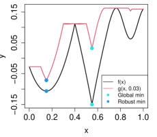
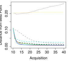
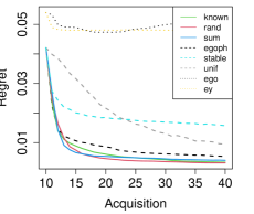
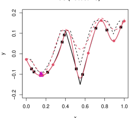
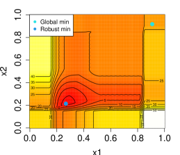
Figure 6 shows a 1d test function of our own creation, first depicted in Figure 1, defined as:

$$f(x)=\begin{cases}3.5(x-0.15)^{2}+\log(1.3)&x<0.4\\ \log(1+|2(x-0.55)|)&0.4\leq x<0.7\\ \frac{1}{20}\sin(25x-17.5)+\log(1.3)&0.7\leq x.\end{cases}$$ (11)

In this problem, $x^{*}=0.55$ and $x^{r}=0.15$ using $\alpha=0.075$. All GP surrogates used $\theta=0.25$. We see a similar story here as for our first test problem. The only notable difference here is that EGO does not get drawn into the peaky region, likely because it is less pronounced. EGO favors sampling around $x^{*}$ initially, but eventually explores the rest of the input space, including around $x^{r}$. Interestingly, REGO with known $\alpha$ performs a little worse than either of the unknown $\alpha$ methods.

Two-dimensional examples

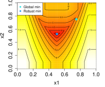
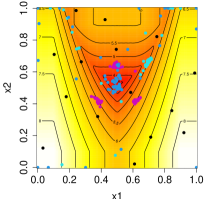
The top-left panel of Figure 7 shows a test problem from Bertsimas et al., (2010), a common test case in robust optimization, which is defined as:

$$f(x_{1},x_{2})=-2x_{1}^{6} +12.2x_{1}^{5}-21.2x_{1}^{4}+6.4x_{1}^{3}+4.7x_{1}^{2}-6.2x_{1}-x_{2}^{6}+11x_{2}^{5}-43.3x_{2}^{4}$$ (12)

$$+74.8x_{2}^{3}-56.9x_{2}^{2}+10x_{2}+4.1x_{1}x_{2}+0.1x_{1}^{2}x_{2}^{2}-0.4x_{1}x_{2}^{2}-0.4x_{1}^{2}x_{2}.$$

Figure 7: Top: The Bertsimas function on the left and the robust surface with $\alpha=0.15$ on the right. Bottom: $d(x^{*}_{\mathrm{b,n}})$ (left) and $r(x^{*}_{\mathrm{b,n}})$ (right) after each acquisition.

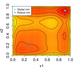
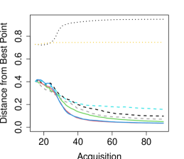
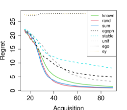
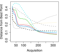
We negated this function compared to Bertsimas et al.,, who were interested in maximization. Originally, it was defined on $x_{1}\in[-0.95,3.2]$ and $x_{2}\in[-0.45,4.4]$ with $x^{*}=(2.8,4.0)$. We coded inputs to $[0,1]^{2}$ so that the true minimum is at $(0.918,0.908)$. In the scaled space, $x^{r}=(0.2673,0.2146)$ using $\alpha=0.15$. We used $N=90$ and $\theta=1.1$. Appendix A considers a variation where $\hat{\theta}$ is re-estimated after each acquisition. The results are very similar, but noisier. The bottom row of panels in Figure 7 show that non-fixed $\alpha$ for REGO can give superior performance in early acquisitions. StableOPT performs worse with this problem because the objective surface near $x^{r}$ is relatively more peaked, say compared to the 1d RKHS example. Regret is trending toward 0 when using BEAR for acquisitions, with REGO-based methods leading the charge. EGO with post hoc adversary performs much worse for this problem. EGO-based acquisitions heavily cluster near $x^{*}$ which thwarts consistent identification of $x^{r}$ even with a post hoc surrogate.

Figure 8: Top: The Bertsimas function on the left with the robust surface with $\alpha=(0.2,0)$ on the right. Bottom: $d(x^{*}_{\mathrm{b,n}})$ (left) and $r(x^{*}_{\mathrm{b,n}})$ (right) after each acquisition.

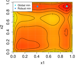
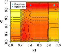
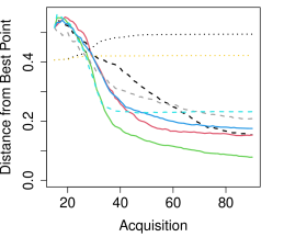
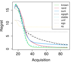
Figure 8 considers the same test problem (12), except this time we use $\alpha=(0.2,0)$, meaning no robustness required in $x_{2}$. This moves $x^{r}$ to $(0.412,0.915)$ in the scaled space. In this problem, the robust surface is fairly flat meaning that when an algorithm finds $x_{2}=0.915$, $x_{1}\in[0.35,0.75]$ gives a similar robust output. For that reason, all of the methods perform worse when trying to pin down the exact $x_{1}$ location, so by looking at metric $d(x^{*}_{\mathrm{b}})$ from Eq. (10), all methods appear to be doing worse, whereas $r(x^{*}_{\mathrm{b}})$ goes to 0 relatively quickly. A shallower robust minimum favors StableOPT. Since that comparator never actually evaluates at $x^{r}$, here it suffices to find $x_{1}\in[0.35,0.75]$, which it does quite easily. Knowing true $\alpha$ for REI helps considerably. This makes sense because omitting an entire dimension from robust consideration is informative. Nevertheless, alternatives using random and aggregate $\alpha$-values perform well.

Higher dimension

Our final set of test functions comes from the Rosenbrock family (Dixon and Szego,, 1979),

$$\sum_{i=1}^{d-1}\left(100(x_{i+1}-x_{i})^{2}+(x_{i}-1)^{2}\right).$$ (13)

defined in arbitrary dimension $d$. Originally in $[-2.48,2.48]^{d}$, we again scale to $[0,1]^{d}$. Although our focus here will be on $d=4$, visualization easier in 2d. Appendix B provides results for a 6d variation, which are quite similar.

Figure 9: Left: 2d log Rosenbrock function on the top and the robust surface with $\alpha=0.1$ on the bottom. Top: $d(x^{*}_{\mathrm{b,n}})$ in the middle and $r(x^{*}_{\mathrm{b,n}})$ on the right for 2d. Bottom: similarly in 4d.

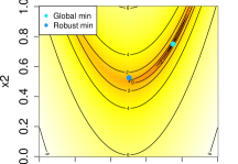
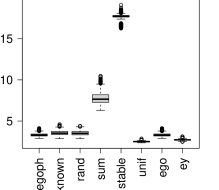
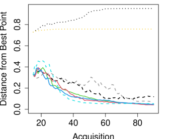
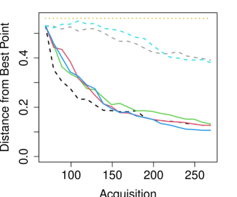
The top-left panel of Figure 9 shows outputs on the log scale (2d). Here $x^{*}=(0.75,0.75)$ and $x^{r}=(0.503,0.525)$ when $\alpha=0.1$. A visual of this adversary is in the bottom-left panel. In 2d, we set $\theta=0.9$ and in 4d, we use $\theta=0.05$. Results for 2d are in the top row (middle and right panels), and for 4d are in the bottom row, respectively. REGO shines in both cases because $x^{*}$ is in a peaked region and $x^{r}$ is in a shallow one. EGO with post hoc adversary does well early on, but stops improving much after about 150 acquisitions. StableOPT has the same issues of sampling around $x^{r}$ that we have seen throughout – never actually sampling it.

4.3 Supplementary empirical analysis

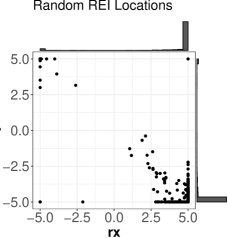
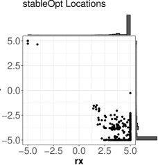
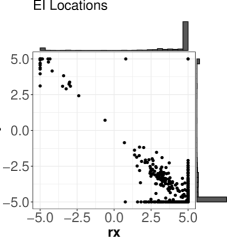
An instructive, qualitative way to evaluate each acquisition algorithm is to inspect the final collection of samples (at $N$), to see visually if things look better for robust variations. Figure 10 shows the final samples of one representative MC iteration for EGO, REGO with random $\alpha$ and StableOPT for 2d Rosenbrock (13) (left panel) and both Bertsimas (12) variations (middle and right panels).

Consider Rosenbrock first. Here, EGO has most of its acquisitions in a mass around $x^{*}$ with a few dispersed throughout the rest of the space. This is exactly what EGO is designed to do: target the global minimum, but still explore other areas. REGO has a similar amount of space-fillingness, but the target cluster is focused on $x^{r}$ rather than $x^{*}$. On the other hand, StableOPT has almost no exploration points. Nearly all of its acquisitions are on the perimeter of a bounding box around $x^{r}$. While StableOPT does a great job of picking out where $x^{r}$ is, intuitively we do not need 70+ acquisitions all right next to each other. Some of those acquisitions could better facilitate learning of the surface by exploring elsewhere.

Figure 10: Sample acquisitions for EGO, REGO with random $\alpha$ and StableOPT for 2d Rosenbrock with $\alpha=0.1$ (left), and Bertsimas functions with $\alpha=0.15$ (middle), and $\alpha=(0.2,0)$ (right).

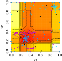
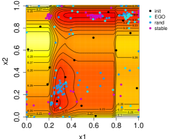
Moving to the Bertsimas panels of the figure, similar behavior may be observed. REGO and EGO have some space-filling points, but mostly target $x^{r}$ for REGO and $x^{*}$ for EGO. StableOPT again puts almost all of its acquisitions near $x^{r}$ with relatively little exploration. But the main takeaway from the Bertsimas plots is that, since REGO does not require setting $\alpha$ beforehand, it gives sensible designs for multiple $\alpha$ values (the blue points are the exactly the same in both panels). Looking more closely at the REGO design, observe that all three minima (global and robust with $\alpha=0.15$ and $\alpha=(0.2,0)$) have many acquisitions around them. This shows the power of REGO, capturing all levels of $\alpha$ and allowing the user to delay specifying $\alpha$ until after experimental design.

Figure 11: Cumulative timings for each method/test function.

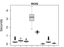
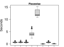
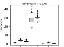
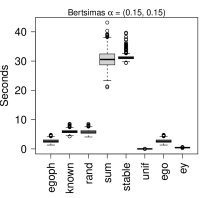
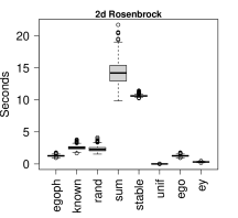
Timings for each method/problem are in Figure 11. Comparators “egoph” and “ego” report identical timings because they involve the same EI acquisition function. As you might expect, “unif” and EY have the lowest times because they do less work. For the more competitive methods, REGO is generally a little slower than EGO, but often faster than StableOPT. The main bottleneck in BO is the $\mathcal{O}(n^{3})$ matrix decomposition(s) required for GP likelihood evaluation and prediction. This $n$ is changing throughout acquisitions, and there is a different final $N$ in each expariment. Consequently we have provided cumulative timings in Figure 11. Since the same underlying GP implementation is shared among all of the competitors in our study, the timings are similar (within the same test problem), with exceptions being “sum” (aggregating many GP fits), “unif” (not requiring a GP), and “stable” (a totally different approach). When amortizing over all $N$ acquisitions, it is clear that each takes just mere seconds even in the worst of cases. We think this is fast enough for most real-world black-box evaluations typically involved in BO enterprises.

5 Robot pushing

Here we consider a real world example to measure the effectiveness of REI. The robot pushing simulator (Kaelbling and Lozano-Perez,, 2017, https://github.com/zi-w/Max-value-Entropy-Search) has been used previously to test ordinary BO (Wang et al.,, 2017; Wang and Jegelka,, 2017) and robust (Bogunovic et al.,, 2018) BO methodology. The simulator models a robot hand, with up to 14 tunable parameters, pushing a box with the goal of minimizing distance to a target location. Following Wang and Jegelka, (2017), we consider varying four of the tunable parameters, as detailed in Table 1.

Parameter	Role	Range
$r_{x}$	initial x-location	$[-5,5]$
$r_{y}$	initial y-location	$[-5,5]$
$r_{\theta}$	initial angle	$[-\frac{\pi}{2},\frac{\pi}{2}]$
$t_{r}$	pushing strength	$[1,30]$

Table 1: Parameters for the robot pushing simulator.

This simulator is coded in Python and uses an engine called Box2D (Catto,, 2011) to simulate the physics of pushing. Also following Wang and Jegelka, (2017), we consider two cases: one with a fixed hand angle, always facing the box, determined to be $r_{\theta}=\arctan(\frac{r_{y}}{r_{x}})$; and the other allowing for all 4 parameters to vary. These create 3d and 4d problems that we call “push3” and “push4”, respectively

We consider two further adaptations. First, we de-noised the simulator, so that it is deterministic, which is more in line with our previous examples. Second, rather than look at a single target location, we take the minimum distance to two, geographically distinct target locations under squared and un-squared distances respectively. We do this in order to manifest a version of the problem that would require robust analysis. Having the box pushed the full distance toward either target, minimizing the objective, yields an output of 0 since $0^{2}=0$. However, the minimum around the unsquared target will be shallower because the unsquared surface increases slower when the distance to the target is greater than 1. Robust BO prefers exploring the unsquared minimum while an ordinary, non-robust method would show no preference. Similarly, a BOV performance metric is indifferent to the target locations, while BEAR would favor the unsquared target.

For both “push3” and “push4” variations, we fixed the target locations at $(-3,3)$ and $(3,-3)$ with the latter being the squared target. Since the unsquared location is in the top-left quadrant, the optimal robust location involves starting the robot hand in the bottom-right so that it pushes the box up and left. Furthermore, because the robot cannot perfectly control the initial hand location, if it is close to the origin, a minor change in $r_{x}$ or $r_{y}$ leads to the hand pushing away from the target location. For “push3” we use $\alpha=0.1$, $x^{r}=(5,-5,25.4)$, meaning the robot hand starts as far in the bottom-right as possible and pushes quite hard. The true setting $g(x^{r},0.1)=1.37$ is lower than analogously pushing toward the squared target location, $g((-5,5,25.4),0.1)=1.88$, solely due to squaring as $1.37^{2}\approx 1.88$.

Figure 12: Results for “push3” $\alpha=0.1$: $d(x^{*}_{\mathrm{b,n}})$ (left), $r(x^{*}_{\mathrm{b,n}})$ (middle) and cumulative time (right).

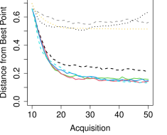
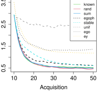
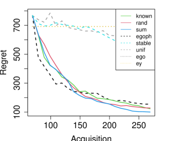
We compare each of the methods from Section 4.2 in a similar fashion by initializing with an LHS of size $n_{0}=10$ and acquiring forty more points ($N=50$), repeating for 1,000 MC samples. Figure 12 summarizes our results. Observe that all of REI variations outperform the others by minimizing regret faster and converging at a lower value. EI with post hoc adversary and StableOPT perform fairly well but suffer from drawbacks similar to those described in Section 4.2. They cannot accommodate squared and unsquared target locations differently.

Figure 13: Distribution of $r_{x}$ and $r_{y}$ from $x^{*}_{\mathrm{bear}}$ for the push3 problem after the final acquisition for “rand” REI using $\alpha=0.1$ (left), StableOPT (middle), and EI (right).

It is worth noting that, while REI performs well, the left panel of Figure 12 suggests that none of the methods are getting very close to always finding $x^{r}$ when $d(x^{*}_{\mathrm{b,n}})=0$. (Distances are not converging to zero.) To dig a little deeper, Figure 13 explores $r_{x}$ and $r_{y}$ from $x^{*}_{\mathrm{bear}}$ for “rand” REI, StableOPT and EI with post hoc adversary. Notice that it is rare for any of these comparators to push toward the “wrong” target location, i.e., finding $(-5,5)$ rather than $(5,-5)$ which would result in large $d(x^{*}_{\mathrm{b,n}})$ and low $r(x^{*}_{\mathrm{b,n}})$. However, EI is attracted to the peaked minimum more often than either of the other methods. REI has this problem slightly more often than StableOPT. However, StableOPT and EI do recommend $x^{*}_{\mathrm{bear}}$ in the bottom-right, but not all the way to $(5,-5)$. This happens more often than with REI. Only occassionally does REI miss entirely, leading to large $d(x^{*}_{\mathrm{b,n}})$. On the other hand, StableOPT identifies the correct area slightly more often, but struggles to pinpoint $x^{r}$. We conclude that both REI and StableOPT perform well – much better than ordinary EI – and any differences are largely a matter of taste or tailoring to specific use cases, modulo computational considerations (right panel).

For “push4”, the location of the robust minimum is the same in that the robot hand starts in the bottom-right, pushing to the top-left. Thus $x_{r}^{*}=(5,-5,-0.79,25.7)$ when using $\alpha=0.1$. Here $g(x_{r}^{*},0.1)=1.64$ compared to $g((-5,5,-0.79,25.7),0.1)=2.71$ by pushing to the squared target location. We again compared the methods from Section 4.2 with 1,000 MC iterations, but this time with an initial LHS of size $n_{0}=20$ and eighty acquisitions ($N=100$). Results are presented in Figure 14. Note that increasing the dimension makes every method do worse, but relative comparisons between methods are similar. Here StableOPT’s performance is better, on par with REI variations, again modulo computing time (right panel).

Figure 14: Results for “push4” $\alpha=0.1$: $d(x^{*}_{\mathrm{b,n}})$ (left), $r(x^{*}_{\mathrm{b,n}})$ (middle) and cumulative time (right).

Figure 15: Distribution of $r_{x}$ and $r_{y}$ from $x^{*}_{\mathrm{bear}}$ for the push4 problem after the final acquisition for random REI using $\alpha=0.1$ (left), StableOPT (middle), and EI (right).

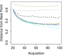
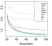
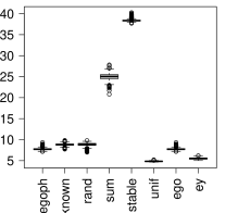
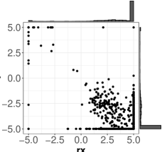
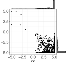
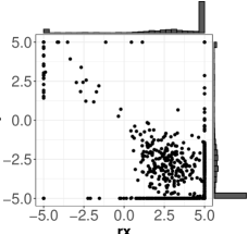
Figure 15 demonstrates the added difficulty “push4”, as indicated by additional spread in the optimal $(r_{x},r_{y})$ compared to Figure 13. This is because a slightly misspecified starting location can be compensated for by adjusting the hand angle. Incorporating that angle introduces a slew of local minima at each $(r_{x},r_{y})$. For example, if we set $r_{x}=3$ rather than 5 as is optimal, and check the regret for “push3” and “push4”, we get $1.1$ and $0.7$, respectively, by changing $r_{\theta}$ to $-0.69$. We may also adjust $t_{r}=24.2$ in both cases to account for the hand being closer to the box. This phenomenon is not unique to the example we chose. Any slight misspecification of $r_{x}$ and $r_{y}$ can be compensated for with a commensurate change in $r_{\theta}$.

To summarize, in contrast to the synthetic examples in Section 4, the results presented here were obtained from a real physics-based simulation. In the 3d variation, REI performs better than all other comparators by finding the minimum in fewer evaluations and its solutions settle on lower distances from the true input location of the robust minimum. In 4d, it’s a closer call: REI performs at least as well as every other non-conventional BO method. The stapleOPT comparator is competitive, modulo trade-offs previously discussed. However, we note that it was not nearly as competitive on synthetic examples.

6 Discussion

We introduced a robust expected improvement (REI) criteria for Bayesian optimization (BO) that provides good experimental designs for targeting robust minima. REI is doubly robust, in a sense, because it is able to accomplish this feat even in cases where one does not know, a priori, the “proper” level of robustness, $\alpha$, to accommodate. In fact, we have shown that in some cases, not fixing the $\alpha$ robustness level beforehand leads to faster discovery of the robust minimum. BO methods, e.g., ordinary EI, miss the robust target entirely. However, by blending EI with an (surrogate modeled) adversary, we are able to get the best of both worlds. Even when designs are not targeted to find a robust minimum, the adversarial surrogate can be applied post hoc to similar effect.

Despite this good empirical performance, the idea of robustness undermines one of the key assumptions of GP regression: stationarity. If one optimum is peaked and another is shallow, then that surface is technically nonstationary. When there are multiple such regimes it can be difficult to pin down lengthscale(s) $\theta$, globally in the input space. Furthermore, $Y^{\alpha}(x)$ can include flat regions which are hard to model with the standard, stationary GP. The underlying REI acquisition scheme may perform even better when equipped with a non-stationary surrogate model such as the treed GP (Gramacy and Lee,, 2007) or a deep GP (Damianou and Lawrence,, 2013; Sauer et al.,, 2022). We surmise that non-GP-based surrogates, e.g., neural networks (Shahriari et al.,, 2020), support vector machines (Shi et al.,, 2020) or random forests (Dasari et al.,, 2019) could be substituted for a GP. Likewise, other acquisition functions can be applied, such as upper-confidence bound (Srinivas et al.,, 2009) or Thompson sampling (Thompson,, 1933), without a fundamental change to the underlying adversarial BO methodology.

Throughout we assumed deterministic $f(x)$. Noise can be accommodated by estimating a nugget parameter. The idea of robustness can be extended to protect against output noise (Beland and Nair,, 2017), in addition to the “input uncertainty” regime we studied here. In that setting, it can be helpful to entertain a heteroskedastic (GP) surrogate (Binois et al.,, 2018, 2019; Binois and Gramacy,, 2019) when the noise level is changing in the input space. We also worked in relatively modest input dimension, with examples on $d\leq 6$. The challenge in working in even higher dimension is two-fold: one is the practical aspect of having a test problem in higher dimension that benefits from a robust approach. The largest real-world example that we could find was the robot pushing problem in 4d. For our 6d work in the supplement we extended the Rosenbrock example from Section 4. The second challenge involves surrogate modeling in higher input dimension, where GPs are known to be data hungry. Yet the whole point of BO is to limit collecting of expensive runs. We are optimistic that recent ideas from the frontier of high dimensional BO would port well to our adversarial framework (Eriksson et al.,, 2020).

Considering that REI/REGO is a multi-step process, and one clearly more involved than ordinary EI/EGO, one may wonder precisely where added value is. The theory for EI/EGO (e.g., Bull,, 2011; Snoek et al.,, 2012a; Bect et al.,, 2016) says that, among other things, eventually you will explore everywhere: an already high level of robustness. That same theory says that EI is optimal for the next acquisition for $f_{n}$, but says nothing futher about the sequence of acquisitions. One can only “hope” that, with a limited budget, EI puts early runs in the right places. That this happens has been illustrated in practice, across many examples and variations, but there is no theory for it. By analogy, REI is optimal for the next acquisition via $\hat{f}_{n}^{\alpha}$, eventually spreading runs everywhere, but one can only “hope” for desirable behavior in the short run, for limited budgets: less seduced by sharp, local mimima but no less exploitative than EI. We illustrated that REI performs desirably on a variety of examples in Sections 4–5.

Like EI/EGO, a theory that guarantees good performance for REI/REGO, under regularity conditions that don’t preclude realistic application (e.g., stationarity, known hyperparameterization, etc.), remains illusive. Both will eventually explore everywhere, but that is an un-inspiring notion of robustness. Perhaps someone smarter than us will come along to fix that. What’s important is “good progress” before reaching “eventually”. This is where BO really shines. Many of the robust methods from the mathematical programming literature – like those cited in Sections 1 and 4.1 – come with attractive theoretical results, at least superficially, like convergence guarantees. However, their empirical performance isn’t competitive under strict evaluation budgets that are common in BO contexts. Perhaps one pays the price for good theory, at least in this context, with poorer performance in practical settings.

Funding

This work was supported by the U.S. Department of Energy, Office of Science, Office of Advanced Scientific Computing Research and Office of High Energy Physics, Scientific Discovery through Advanced Computing (SciDAC) program under Award Number 0000231018.

Appendix A REI with estimated lengthscale

Our experiments in Sections 4.2 and in Section 5 used fixed lengthscales $\theta$ to control MC variability. We did that so that the focus of those experiments to be on the acquisition criteria behind the BO algorithms, not on the surrogate modeling details – which are shared identically among all the methods. However, it is worth wondering how those results might change when lengthscales are re-estimated after each acquisition.

Figure 16: Results for 2d Bertsimas function with $\hat{\theta}$ estimated via MLE: $d(x^{*}_{\mathrm{b,n}})$ (left) and $r(x^{*}_{\mathrm{b,n}})$ (right).

The results in Figure 16 show the Bertsimas function (from Section 4.2) with $\alpha=0.15$ in each dimension, akin to Figure 7. Each $\hat{\theta}$ is calculated by numerically maximizing the likelihood (i.e., MLE) of the multivariate normal log likelihood for the surrogate, and the adversarial surrogate as necessary. The results are very similar to the fixed-$\theta$ case, but they are noisier due to the estimation risk in inferring these additional hyperparamers. In particular, although REI methods perform relatively worse compared to fixed $\theta$ case in Figure 7, they are still winning in comparison to the other methods.

Appendix B REI in higher input dimension

Figure 17 shows the results for the 6d Rosenbrock function, continuing from Figure 9 in Section 4. We use the same setup as the 4d problem, described therein, in particular with $\alpha=0.1$ for every input coordinate. For the initial setup of the 6d problem, we included a point within 0.02 of the global, peaked minimum in each dimension. This is not necessary in general, however in this high dimensional space it is very difficult to locate the global, spiky optimum. By nudging all solvers toward discovering this area, we are better able showcase the merits of our robust solution, which are designed not to be fooled by the spiky solutions.

Figure 17: The results for the 6d Rosenbrock function: $d(x^{*}_{\mathrm{b,n}})$ (left) and $r(x^{*}_{\mathrm{b,n}})$ (right).

Adding this additional design point represents a “temptation” for the conventional, non-robust BO methods, drawing them towards the global minimum over the robust minimum. Without it, the non-robust methods rarely find the global minimum since the surface is so peaked and thus those methods often report the robust minimum erroneously. We see this as short-circuiting the outcome of a much more exhaustive search. I.e., illustrating how each of the methods would perform in the long run, wherein eventually the non-robust methods would be enticed by the global minimum and that would lead to worse acquisitions. Under this setup, and pretty much identically to the 4d example in Section 4/Figure 9, the REI methods are performing the best by both metrics: they are finding the robust minimum faster than the other methods.

References

- Abrahamsen, (1997) Abrahamsen, P. (1997). “A review of Gaussian random fields and correlation functions.” Norsk Regnesentral/Norwegian Computing Center Oslo, https://www.nr.no/directdownload/917_Rapport.pdf.
- Assael et al., (2014) Assael, J.-A. M., Wang, Z., Shahriari, B., and de Freitas, N. (2014). “Heteroscedastic Treed Bayesian Optimisation.” ArXiv.
- Bect et al., (2016) Bect, J., Bachoc, F., and Ginsbourger, D. (2016). “A supermartingale approach to Gaussian process based sequential design of experiments.” Preprint on arXiv:1608.01118.
- Beland and Nair, (2017) Beland, J. J. and Nair, P. B. N. (2017). “Bayesian optimisation under uncertainty.” NIPS BayesOPT 2017 workshop.
- Bertsimas and Nohadani, (2010) Bertsimas, D. and Nohadani, O. (2010). “Robust optimization with simulated annealing.” J. Global Optimization, 48, 323–334.
- Bertsimas et al., (2010) Bertsimas, D., Nohadani, O., and Teo, K. M. (2010). “Robust Optimization for Unconstrained Simulation-Based Problems.” Operations Research, 58, 161–178.
- Bertsimas et al., (2019) Bertsimas, D., Sim, M., and Zhang, M. (2019). “Adaptive Distributionally Robust Optimization.” Management Science, 65, 2, 604–618.
- Binois and Gramacy, (2019) Binois, M. and Gramacy, R. (2019). hetGP: Heteroskedastic Gaussian process modeling and design under replication. R package version 1.1.1.
- Binois et al., (2018) Binois, M., Gramacy, R., and Ludkovski, M. (2018). “Practical heteroscedastic Gaussian process modeling for large simulation experiments.” Journal of Computational and Graphical Statistics, 27, 4, 808–821.
- Binois et al., (2019) Binois, M., Huang, J., Gramacy, R., and Ludkovski, M. (2019). “Replication or exploration? Sequential design for stochastic simulation experiments.” Technometrics, 27, 4, 808–821.
- Bisschop and Entriken, (1993) Bisschop, J. and Entriken, R. (1993). AIMMS : The Modeling System. Paragon Decision Technology B.V.
- Blum and Mansour, (2007) Blum, A. and Mansour, Y. (2007). “Learning, Regret minimization, and Equilibria.” In Algorithmic Game Theory, eds. N. Nisan, T. Roughgarden, E. Tardos, and V. V. Vazirani, chap. 4, 79–103. New York, NY, USA: Cambridge University Press.
- Bogunovic et al., (2018) Bogunovic, I., Scarlett, J., Jegelka, S., and Cevher, V. (2018). “Adversarially Robust Optimization with Gaussian Processes.” Advances in Neural Information Processing Systems, 31, 5760–5770.
- Box and Draper, (2007) Box, G. and Draper, N. (2007). Response Surfaces, Mixtures, and Ridge Analyses, vol. 649. John Wiley & Sons.
- Bull, (2011) Bull, A. (2011). “Convergence rates of efficient global optimization algorithms.” Journal of Machine Learning Research, 12, Oct, 2879–2904.
- Burden and Faires, (1989) Burden, R. L. and Faires, J. D. (1989). Numerical Analysis. The Prindle, Weber and Schmidt Series in Mathematics, 4th ed. Boston: PWS-Kent Publishing Company.
- Byrd et al., (1995) Byrd, R. H., Lu, P., Nocedal, J., and Zhu, C. (1995). “A Limited Memory Algorithm for Bound Constrained Optimization.” SIAM Journal on Scientific Computing, 16, 5, 1190–1208.
- Catto, (2011) Catto, E. (2011). “Box2D, a 2D physics engine for games.”
- Cheney and Goldstein, (1959) Cheney, E. W. and Goldstein, A. A. (1959). “Newton’s Method for Convex Programming and Tchebycheff Approximation.” Numer. Math., 1, 1, 253–268.
- Conn and Vicente, (2012) Conn, A. and Vicente, L. (2012). “Bilevel derivative-free optimization and its application to robust optimization.” Optimization Methods and Software, 27, 561–577.
- Damianou and Lawrence, (2013) Damianou, A. and Lawrence, N. D. (2013). “Deep Gaussian Processes.” In Proceedings of the Sixteenth International Conference on Artificial Intelligence and Statistics, eds. C. M. Carvalho and P. Ravikumar, vol. 31 of Proceedings of Machine Learning Research, 207–215. Scottsdale, Arizona, USA: PMLR.
- Dasari et al., (2019) Dasari, S. K., Cheddad, A., and Andersson, P. (2019). “Random Forest Surrogate Models to Support Design Space Exploration in Aerospace Use-Case.” In Artificial Intelligence Applications and Innovations, eds. J. MacIntyre, I. Maglogiannis, L. Iliadis, and E. Pimenidis, 532–544. Cham: Springer International Publishing.
- Dean et al., (2015) Dean, A., Morris, M., Stufken, J., and Bingham, D. (2015). Handbook of Design and Analysis of Experiments. Chapman & Hall/CRC Handbooks of Modern Statistical Methods. CRC Press.
- Dixon and Szego, (1979) Dixon, L. C. W. and Szego, G. P. (1979). The global optimization problem: an introduction. Amsterdam: North-Holland Pub. Co.
- Dunning et al., (2017) Dunning, I., Huchette, J., and Lubin, M. (2017). “JuMP: A Modeling Language for Mathematical Optimization.” SIAM Review, 59, 2, 295–320.
- Eriksson et al., (2020) Eriksson, D., Pearce, M., Gardner, J. R., Turner, R., and Poloczek, M. (2020). “Scalable Global Optimization via Local Bayesian Optimization.”
- Goerigk, (2014) Goerigk, M. (2014). “ROPI - a robust optimization programming interface for C++.” Optim. Methods Softw., 29, 6, 1261–1280.
- Goh and Sim, (2009) Goh, J. and Sim, M. (2009). “Robust optimization made easy with ROME.” Operations Research, 59, 973–985.
- Goldfarb and Iyengar, (2003) Goldfarb, D. and Iyengar, G. (2003). “Robust Portfolio Selection Problems.” Mathematics of Operations Research, 28, 1, 1–38.
- Gramacy, (2016) Gramacy, R. B. (2016). “laGP : Large-Scale Spatial Modeling via Local Approximate Gaussian Processes in R.” Journal of Statistical Software, 72.
- Gramacy, (2020) — (2020). Surrogates: Gaussian Process Modeling, Design and Optimization for the Applied Sciences. Boca Raton, Florida: Chapman Hall/CRC.
- Gramacy and Lee, (2007) Gramacy, R. B. and Lee, H. K. H. (2007). “Bayesian treed Gaussian process models with an application to computer modeling.”
- Gramacy et al., (2022) Gramacy, R. B., Sauer, A., and Wycoff, N. (2022). “Triangulation candidates for Bayesian optimization.”
- Hong and Nelson, (2006) Hong, L. and Nelson, B. (2006). “Discrete optimization via simulation using COMPASS.” Operations Research, 54, 115–129.
- Huang et al., (2011) Huang, L., Joseph, A., Nelson, B., Rubinstein, B. I. P., and Tygar, J. (2011). “Adversarial machine learning.” In AISec ’11, ed. Y. Chen.
- Jones et al., (1998) Jones, D., Schonlau, M., and Welch, W. (1998). “Efficient Global Optimization of Expensive Black-Box Functions.” Journal of Global Optimization, 13, 455–492.
- Kaelbling and Lozano-Perez, (2017) Kaelbling, L. and Lozano-Perez, T. (2017). “Learning composable models of parameterized skills.” In 2017 IEEE International Conference on Robotics and Automation (ICRA), 886–893.
- Kaelbling et al., (1996) Kaelbling, L. P., Littman, M. L., and Moore, A. W. (1996). “Reinforcement leaarning: A survey.” Journal of Artificial Intelligence Research, 4, 237–285.
- Kalpić and Hlupić, (2011) Kalpić, D. and Hlupić, N. (2011). Multivariate Normal Distributions, 907–910. Berlin, Heidelberg: Springer Berlin Heidelberg.
- Kolvenbach et al., (2018) Kolvenbach, P., Lass, O., and Ulbrich, S. (2018). “An approach for robust PDE-constrained optimization with application to shape optimization of electrical engines and of dynamic elastic structures under uncertainty.” Optimization and Engineering, 19, 1–35.
- Leyffer et al., (2020) Leyffer, S., Menickelly, M., Munson, T., Vanaret, C., and Wild, S. M. (2020). “A survey of nonlinear robust optimization.” INFOR: Information Systems and Operational Research, 58, 2, 342–373.
- Li et al., (2002) Li, W., Huyse, L., and Padula, S. (2002). “Robust airfoil optimization to achieve drag reduction over a range of mach numbers.” Structural and Multidisciplinary Optimization, 24, 38–50.
- Löfberg, (2008) Löfberg, J. (2008). “Modeling and solving uncertain optimization problems in YALMIP.” IFAC Proceedings Volumes, 41, 2, 1337–1341. 17th IFAC World Congress.
- Martinez-Cantin et al., (2009) Martinez-Cantin, R., Freitas, N., Brochu, E., Castellanos, J., and Doucet, A. (2009). “A Bayesian exploration-exploitation approach for optimal online sensing and planning with a visually guided mobile robot.” Auton. Robots, 27, 93–103.
- Marzat et al., (2016) Marzat, J., Walter, E., and Piet-Lahanier, H. (2016). “A new expected-improvement algorithm for continuous minimax optimization.” J. Glob. Optim., 64, 4, 785–802.
- Menickelly and Wild, (2018) Menickelly, M. and Wild, S. M. (2018). “Derivative-free robust optimization by outer approximations.” Mathematical Programming, 179, 1-2.
- Menickelly and Wild, (2020) — (2020). “Derivative-Free Robust Optimization by Outer Approximations.” Mathematical Programming, 179, 1–2, 157–193.
- Mockus et al., (1978) Mockus, J., Tiesis, V., and Zilinskas, A. (1978). “The application of Bayesian methods for seeking the extremum.” Towards Global Optimization, 2, 117-129, 2.
- Myers et al., (2016) Myers, R., Montgomery, D., and Anderson-Cook, C. (2016). Response Surface Methodology: Process and Product Optimization Using Designed Experiments. John Wiley & Sons.
- Neal, (1998) Neal, R. (1998). “Regression and classification using Gaussian process priors.” Bayesian Statistics, 6, 475.
- Nogueira et al., (2016) Nogueira, J., Martinez-Cantin, R., Bernardino, A., and Jamone, L. (2016). “Unscented Bayesian Optimization for Safe Robot Grasping.” CoRR, abs/1603.02038.
- Oliveira et al., (2019) Oliveira, R., Ott, L., and Ramos, F. (2019). “Bayesian optimisation under uncertain inputs.” In Proceedings of the Twenty-Second International Conference on Artificial Intelligence and Statistics, eds. K. Chaudhuri and M. Sugiyama, vol. 89 of Proceedings of Machine Learning Research, 1177–1184. PMLR.
- R Core Team, (2021) R Core Team (2021). R: A Language and Environment for Statistical Computing. R Foundation for Statistical Computing, Vienna, Austria.
- Randall et al., (1981) Randall, S. E., Halsted, D. M., I., and Taylor, D. L. (1981). “Optimum Vibration Absorbers for Linear Damped Systems.” Journal of Mechanical Design, 103, 4, 908–913.
- Rasmussen and Williams, (2006) Rasmussen, C. and Williams, C. (2006). Gaussian Processes for Machine Learning. Cambridge, MA: MIT Press.
- Sacks et al., (1989) Sacks, J., Welch, W. J., Mitchell, T. J., and Wynn, H. P. (1989). “Design and Analysis of Computer Experiments.” Statistical Science, 4, 4, 409–423.
- Santner et al., (2018) Santner, T., Williams, B., and Notz, W. (2018). The Design and Analysis of Computer Experiments, Second Edition. New York, NY: Springer–Verlag.
- Sauer et al., (2022) Sauer, A., Cooper, A., and Gramacy, R. B. (2022). “Vecchia-approximated Deep Gaussian Processes for Computer Experiments.”
- Scott et al., (2011) Scott, W., Frazier, P., and Powell, W. (2011). “The Correlated Knowledge Gradient for Simulation Optimization of Continuous Parameters using Gaussian Process Regression.” SIAM Journal on Optimization, 21, 996–1026.
- Shahriari et al., (2016) Shahriari, B., Swersky, K., Wang, Z., Adams, R. P., and de Freitas, N. (2016). “Taking the Human Out of the Loop: A Review of Bayesian Optimization.” Proceedings of the IEEE, 104, 1, 148–175.
- Shahriari et al., (2020) Shahriari, M., Pardo, D., Moser, B., and Sobieczky, F. (2020). “A Deep Neural Network as Surrogate Model for Forward Simulation of Borehole Resistivity Measurements.” Procedia Manufacturing, 42, 235–238. International Conference on Industry 4.0 and Smart Manufacturing (ISM 2019).
- Shi et al., (2020) Shi, M., Lv, L., Sun, W., and Song, X. (2020). “A Multi-Fidelity Surrogate Model Based on Support Vector Regression.” Struct. Multidiscip. Optim., 61, 6, 2363–2375.
- Snoek et al., (2012a) Snoek, J., Larochelle, H., and Adams, R. (2012a). “Practical Bayesian optimization of machine learning algorithms.” In Advances in Neural Information Processing Systems, 2951–2959.
- Snoek et al., (2012b) Snoek, J., Larochelle, H., and Adams, R. P. (2012b). “Practical Bayesian optimization of machinelearning algorithms.” Advances in Neural information Processing Systems (NIPS), 2951–2959.
- Srinivas et al., (2009) Srinivas, N., Krause, A., Kakade, S., and Seeger, M. (2009). “Gaussian process optimization in the bandit setting: no regret and experimental design.” Preprint on arXiv:0912.3995.
- Stein, (1999) Stein, M. L. (1999). Interpolation of spatial data. Springer-Verlag.
- Taddy et al., (2009) Taddy, M. A., Lee, H. K. H., Gray, G. A., and Griffin, J. D. (2009). “Bayesian Guided Pattern Search for Robust Local Optimization.” Technometrics, 51, 4, 389–401.
- Taguchi, (1986) Taguchi, G. (1986). Introduction to quality engineering: designing quality into products and processes.
- Thompson, (1933) Thompson, W. (1933). “On the likelihood that one unknown probability exceeds another in view of the evidence of two samples.” Biometrika, 25, 3/4, 285–294.
- Vanchinathan et al., (2014) Vanchinathan, H. P., Nikolic, I., De Bona, F., and Krause, A. (2014). “Explore-Exploit in Top-N Recommender Systems via Gaussian Processes.” In Proceedings of the 8th ACM Conference on Recommender Systems, eds. A. Kobsa and M. Zhou, RecSys ’14, 225–232. Association for Computing Machinery.
- Vayanos et al., (2022) Vayanos, P., Jin, Q., and Elissaios, G. (2022). “ROC++: Robust Optimization in C++.” INFORMS Journal on Computing, 34, 6, 2873–2888.
- Vaz and Fernandes, (2006) Vaz, I. and Fernandes, E. (2006). “Solving semi-infinite programming problems by using an interface between MATLAB and SIPAMPL.” ACM Trans Math Softw., 283–288.
- Wang and Jegelka, (2017) Wang, Z. and Jegelka, S. (2017). “Max-Value Entropy Search for Efficient Bayesian Optimization.” In Proceedings of the 34th International Conference on Machine Learning - Volume 70, ICML’17, 3627–3635. JMLR.org.
- Wang et al., (2017) Wang, Z., Li, C., Jegelka, S., and Kohli, P. (2017). “Batched High-dimensional Bayesian Optimization via Structural Kernel Learning.” In Proceedings of the 34th International Conference on Machine Learning, eds. D. Precup and Y. W. Teh, vol. 70 of Proceedings of Machine Learning Research, 3656–3664. PMLR.
- Zhang et al., (2020) Zhang, B., Cole, D., and Gramacy, R. (2020). “Distance-distributed design for Gaussian process surrogates.” To appear in Technometrics. Preprint on arXiv:1812.02794.