Jet SIFT-ing:
a new scale-invariant jet clustering algorithm for the substructure era

Abstract

We introduce a new jet clustering algorithm named SIFT (Scale-Invariant Filtered Tree) that maintains the resolution of substructure for collimated decay products at large boosts. The scale-invariant measure combines properties of $k_{\textrm{T}}$ and anti-$k_{\textrm{T}}$ by preferring early association of soft radiation with a resilient hard axis, while avoiding the specification of a fixed cone size. Integrated filtering and variable-radius isolation criteria block assimilation of soft wide-angle radiation and provide a halting condition. Mutually hard structures are preserved to the end of clustering, automatically generating a tree of subjet axis candidates. Excellent object identification and kinematic reconstruction for multi-pronged resonances are realized across more than an order of magnitude in transverse energy. The clustering measure history facilitates high-performance substructure tagging, which we quantify with the aid of supervised machine learning. These properties suggest that SIFT may prove to be a useful tool for the continuing study of jet substructure.

I Introduction

The collider production of an isolated partonic object bearing uncanceled strong nuclear charge is immediately followed by a frenzied showering of soft and collinear radiation with a complex process of recombination into meta-stable color-singlet hadronic states. In order to compare theoretical predictions for hard scattering events against experimental observations, it is necessary to systematically reassemble these “jets” of fragmentary debris into a faithful representation of their particle source. The leading clustering algorithm serving this purpose at the Large Hadron Collider (LHC) is anti-$k_{\textrm{T}}$ [1], which is valued for yielding regular jet shapes that are simple to calibrate.

It can often be the case that clustering is complicated by early decays of a heavy unstable state into multiple hard prongs, e.g., as $(W^{+}\to u\,\bar{d})$, or $(t\to W^{+}b\to u\,\bar{d}\,b)$. This additional structure can be of great benefit for tagging presence of the heavy initial state. However, identification will be confounded if essential constituents of distinct prongs either remain uncollected, or are merged together into a joint assemblage. Standard practice is to err in the latter direction, via construction of a large-radius jet that is intended to encapsulate all relevant showering products, and to subsequently attempt recovery of the lost “substructure” using a separate algorithm such as $N$-subjettiness [2].

The casting of this wide net invariably also sweeps up extraneous low-energy radiation at large angular separations and successful substructure tagging typically hinges on secondarily “grooming” large-radius jets with a technique such as Soft Drop [3]. Furthermore, the appropriate angular coverage is intrinsically dependent upon the process being investigated, since more boosted parents will tend to produce more collimated beams of children. Accordingly, such methods are conventionally tuned to target specific energy scales for maximal efficacy.

In this paper, we introduce a new jet clustering algorithm called SIFT (Scale-Invariant Filtered Tree) that is engineered to avoid losing resolution of structure in the first place. Similar considerations previously motivated development of the exclusive XCone [4, 5] algorithm based on minimization of $N$-jettiness [6]. Most algorithms in common use reference a fixed angular cone size $R_{0}$, inside of which all presented objects will cluster, and beyond which all exterior objects will be excluded. We identify this parameter, and the conjugate momentum scale which it imprints, as primary culprits responsible for the ensuing loss of resolution.

In keeping, our proposal rejects any such references to an external scale, while asymptotically recovering successful angular and kinematic behaviors of algorithms in the $k_{\textrm{T}}$-family. Specifically, the SIFT prioritizes pairing objects that have hierarchically dissimilar transverse momentum scales (i.e., one member is soft relative to its partner), and narrow angular separation (i.e., the members are collinear). The form we are lead to by these considerations is quite similar to a prior clustering measure named Geneva [7], although our principal motivation (retention of substructure) differs substantively from those that applied historically.

We additionally resolve a critical fault that otherwise precludes the practical application of radius-free measures such as Geneva, namely the tendency to gather uncorrelated soft radiation at wide angular separations. This is accomplished with a novel filtering and halting prescription that is motivated by Soft Drop, but defined in terms of the scale-invariant measure itself and applied to each candidate merger during the initial clustering.

The final-state objects retained after algorithm termination are isolated variable-large-radius jets that dynamically bundle decay products of massive resonances in response to the process scale. Since mutually hard prongs tend to merge last (this behavior is very different from that of anti-$k_{\textrm{T}}$), the end stages of clustering densely encode information indicating the presence of substructure. Accordingly, we introduce the concept of an $N$-subjet tree, which represents the ensemble of a merged object’s projections onto $N$ axes, as directly associated with the clustering progression from $N$ prongs to $1$.

We demonstrate that the subjet axes obtained in this manner are effective for applications such as the computation of $N$-subjettiness. Additionally, we confirm that they facilitate accurate and sharply-peaked reconstruction of associated mass resonances. Finally, we show that the sequential evolution history of the SIFT measure across mergers is itself an excellent substructure discriminant. As quantified with the aid of a Boosted Decision Tree (BDT), we find that it significantly outperforms the benchmark approach to distinguishing one-, two-, and three-prong events using $N$-subjettiness ratios, especially in the presence of a large transverse boost.

The outline of this work is as follows. Section II presents a master sequential jet clustering algorithm into which SIFT and the $k_{\textrm{T}}$ prescriptions may be embedded. Sections III–VI define the SIFT algorithm in terms of its scale-invariant measure (with transformation to a coordinate representation), filtering and isolation criteria, and final-state $N$-subjet tree objects. Section VII visually contrasts clustering priorities, soft radiation catchment, and halting status against common algorithms. Sections VIII–IX comparatively assesses SIFT’s performance in various applications, relating firstly to jet resolution and mass reconstruction, and secondly to the tagging of structure. Section X addresses computability, infrared and collinear safety, and $\mathcal{O}(1)$ deviations from recursive safety. Section XI concludes and summarizes. Appendix A provides a pedagogical review of hadron collider coordinates. Appendix B describes available software implementations of the SIFT algorithm along with methods for reproducing current results and plans for integration with the FastJet [8, 9] contributions library.

II The Master Algorithm

Figure 1: Generalized logical flow chart representing a family of sequential jet clustering algorithms defined by a distance measure $\delta_{AB}$, along with a specification for filtering and isolation criteria and/or a target final-state jet count for exclusive clustering.

This section summarizes the global structure of a general sequential jet clustering algorithm, as illustrated in FIG. 1. Examples are provided of how standard algorithms fit into this framework. These examples will be referenced subsequently to motivate the SIFT algorithm and to comparatively assess its performance.

To begin, a pool of $N$ low-level physics objects (e.g., four-vector components of track-assisted calorimeter hits) is populated, typically including reconstructed hadrons as well as photons and light leptons that fail applicable hardness, identification, or isolation criteria.

The main loop then begins by finding the two most-proximal objects ($A,B$), as defined via minimization of a specified distance measure $\delta_{AB}$ over each candidate pairing. For example, the anti-$k_{\textrm{T}}$ algorithm is a member (with index $n=-1$) of a broader class of algorithms that includes the earlier $k_{\textrm{T}}$ [10, 11] (with $n=+1$) and Cambridge-Aachen [12, 13] (with $n=0$) formulations, corresponding to the measure $\delta_{AB}^{k_{\rm T},n}$ defined as:

$$\delta_{AB}^{k_{\rm T},n}\equiv{\rm min}\bigg{[}\,{\left(p_{\textrm{T}}^{A}\right)}^{2n}\!\!,\,{\left(p_{\textrm{T}}^{B}\right)}^{2n}\,\bigg{]}\times{\left(\frac{\Delta R_{AB}}{R_{0}}\right)}^{\!2}$$ (1)

The quantity ${(\Delta R_{AB})}^{2}\equiv{(\Delta\eta)}^{2}+{(\Delta\phi)}^{2}$ expresses “geometric” adjacency as a Cartesian norm-square of differences in pseudo-rapidity $\eta$ and azimuthal angle $\phi$ (cf. Appendix A) relative to the maximal cone radius $R_{0}$. The $(n=0)$ scenario prioritizes small values of $\Delta R_{AB}$ without reference to the transverse momentum $p_{\textrm{T}}$. A positive momentum exponent $(n=+1)$ first associates pairs wherein at least one member is very soft, naturally rewinding the chronology of the showering process. A negative momentum exponent $(n=-1)$ favors pairs wherein at least one member represents hard radiation directed away from the beamline.

Once an object pair has been selected, there are various ways to handle its members. Broadly, three useful alternatives are available, identified here as clustering, dropping, and isolating. The criteria for distinguishing between these actions are an important part of any algorithm’s halting condition. Clustering means that the objects ($A,B$) are merged, usually via a four-vector sum ($p^{\mu}_{AB}=p^{\mu}_{A}+p^{\mu}_{B}$), and replaced by this merged object in the pool. Typically, clustering proceeds unless the applicable angular separation is too great and/or the momentum scales of the members are too dissimilar.

For pairings failing this filter, two options remain. Dropping, wherein the softer member is set aside (it may literally be discarded or rather reclassified as a final-state object) while the harder member is returned to the object pool, sensibly applies when momentum scales are hierarchically imbalanced. Conversely, a symmetric treatment of both members is motivated when momentum scales are similar, and isolating involves mutual reclassification as final-state objects. Exclusive algorithms (which guarantee a fixed ending count $N_{\rm exc}$ of jets) typically always cluster, although any construction that reduces the net object count by one unit per iteration is consistent.

To complete the prior example, conventional implementations of $k_{\textrm{T}}$-family clustering do not discard objects or collectively isolate final-state pairs. However, they do singly reclassify all objects with no partners nearer than $R_{0}$ in $\Delta R$ as final-state jets. This behavior may be conveniently embedded into the master algorithm flow by also allowing each object in the active pool to pair one at a time with the “beam” and associating it with the alternative measure $\delta_{\rm beam}^{k_{\rm T},n}=p_{\textrm{T}}^{2n}$. The dropping criterion is then adapted to set aside any object for which this beam distance is identified as the global minimum. Note that such objects are indeed guaranteed to have no neighbors inside a centered cone of size $R_{0}$.

The described loop repeats until the number of objects remaining in the active pool reaches a specified threshold. In the context of an exclusive clustering mode this would correspond to a target count $N_{\rm exc}$, whereas continuation otherwise simply requires the presence of multiple ($N>1$) objects. Many clustering algorithms, including SIFT, may be operated in either of these modes. Upon satisfaction of the halting criteria, the list of final-state objects is returned along with a record of the clustering sequence and associated measure history.

The SIFT algorithm will now be systematically developed by providing specific prescriptions for each element of the master algorithm. The scale-invariant measure $\delta_{AB}$ is defined in Section III and provided with an intuitive geometric form in Section IV. The filtering and isolation criteria are itemized in Section V. The $N$-subjet tree is introduced in Section VI.

III The Scale-Invariant Measure 

This section establishes the SIFT clustering measure $\delta_{AB}$ and places it in the context of similar constructs from the literature. Our principal objective is to develop an approach that is intrinsically resilient against loss of substructure in boosted event topologies, i.e., which maintains resolution of collimated radiation associated with distinct partonic precursors in the large-$p_{\textrm{T}}$ limit.

We identify specification of an angular size parameter $R_{0}$ as the primary culprit imposing a conjugate momentum scale dependence on the performance of traditional approaches to jet clustering. In pursuit of a scale-independent algorithm, we require that the clustering measure be free of any such factor. Nevertheless, it is desirable to asymptotically recover angular and kinematic characteristics of existing successful approaches such as anti-$k_{\textrm{T}}$ (cf. Eq. 1 with $n=-1$), and we thus seek out proxies for its dominant behaviors. Specifically, these include a preference for pairs with close angular proximity, and a preference for pairs where one member carries a large transverse boost. For the former purpose, we invoke the mass-square difference, defined as follows:

$$\Delta m_{AB}^{2} \equiv(p^{\mu}_{A}+p^{\mu}_{B})^{2}-m_{A}^{2}-m_{B}^{2}\,=\,2p^{\mu}_{A}p_{\mu}^{B}$$ (2)

$$\simeq 2E^{A}E^{B}\times(1-\cos\Delta\theta_{AB})\simeq E^{A}E^{B}\Delta\,\theta_{AB}^{2}$$

The property that small mass-square changes correlate with collinearity of decay products was similarly leveraged by the early JADE [14] algorithm. For the latter purpose, we turn to suppression in a denominator by the summed transverse energy-square:

$${\textstyle\sum}\,E_{\textrm{T}}^{2} \equiv(E_{\textrm{T}}^{A})^{2}+(E_{\textrm{T}}^{B})^{2}$$ (3)

$$E_{\textrm{T}}^{2} \equiv p_{\textrm{T}}^{2}+m^{2}=E^{2}-p_{z}^{2}$$

The summation plays a role similar to that of the “min” criterion in Eq. (1), in the case that the pair of objects under consideration is very asymmetrically boosted. The choice of $E_{\textrm{T}}^{2}$ over simply $p_{\textrm{T}}^{2}$ prevents a certain type of divergence, as it is possible for the vector quantity $\vec{p}_{\rm T}$ to cancel during a certain phase of the clustering, but not without generation of mass. All together, the simple prescription for the proposed algorithm is to sequentially cluster indexed objects $A$ and $B$ corresponding to the smallest pairwise value of the following expression:

$$\delta_{AB}\equiv\frac{\Delta m_{AB}^{2}}{(E_{\textrm{T}}^{A})^{2}+(E_{\textrm{T}}^{B})^{2}}$$ (4)

Since this measure represents our default context, we write it without an explicit superscript label for simplicity. We note that it consists of the dimensionless ratio of a Lorentz invariant and an invariant under longitudinal boosts, and that it manifestly possesses the desired freedom from arbitrary externally-specified scales. For comparison, the JADE clustering measure is:

$$\delta_{AB}^{\rm JADE}\equiv\frac{E_{A}E_{B}}{s}\times\left(1-\cos\Delta\theta_{AB}\right)$$ (5)

Having been designed for application at a lepton collider, JADE [15] references total energies ($E_{A},E_{B}$) and spherically symmetric angular separations $\Delta\theta_{AB}$ rather than cylindrical quantities. It also treats all merger candidates as massless, i.e., it uniformly factors ($|\vec{p}|\Rightarrow E$) out of the angular dependence. Although Eq. (5) is dimensionless and avoids referencing a fixed cone size, it is not scale-invariant, due to normalization against the global Mandelstam center-of-momentum energy $\sqrt{s}$. This distinction is amplified in a hadron collider context, where the partonic $\sqrt{\hat{s}}$ and laboratory center-of-momentum frames are generally not equivalent.

However, the historical measure most alike to SIFT is Geneva, which was developed as a modification to JADE:

$$\delta_{AB}^{\rm Geneva}\equiv\frac{8}{9}\frac{E_{A}E_{B}}{{(E_{A}+E_{B})}^{2}}\times\left(1-\cos\Delta\theta_{AB}\right)$$ (6)

Like Eq. (4), Eq. (6) achieves scale-invariance by constructing its denominator from dimensionful quantities local to the clustering process. There are also several differences between the two forms, which are summarized here and explored further in Section IV. Variations in the dimensionless normalization are irrelevant. The substitution of cylindrical for spherical kinematic quantities is relevant, albeit trivial. Exchanging the squared sum for a sum of squares causes the SIFT measure fall off more sharply than the Geneva measure as the momentum scales of the clustering candidates diverge. But, the most critical distinguishing feature is that SIFT is sensitive to accumulated mass.

Despite core similarities at measure level, the novel filtering and isolation criteria described in Section V are responsible for essential divergences in the properties of final-state objects produced by SIFT relative to those from Geneva. In particular, we will show that the $N$-subjet tree introduced in Section VI is effective for reconstructing hard objects and tagging the presence of substructure at large transverse boosts without the need for additional de/reclustering or post-processing.

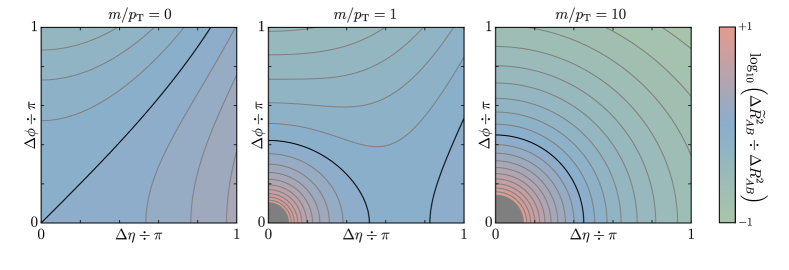
Figure 2: The factor $\Delta\widetilde{R}^{2}_{AB}$ is compared to the traditional angular measure $\Delta R^{2}_{AB}$, as a function of $\Delta\eta$ and $\Delta\phi$, and for various values of ($m/p_{\textrm{T}}$). Regions where the SIFT measure enhances (suppresses) clustering are shown in green (red). Blue indicates similar behavior, with black contour placed at unity. Grey contours mark increments of $0.1$ in $\log_{10}(\Delta\widetilde{R}^{2}_{AB}\div\Delta R^{2}_{AB})$.

IV The Geometric Form

This section presents a transformation of the SIFT clustering measure into the geometric language of coordinate differences. While the underlying physics is invariant under this change of variables, the resulting expression is better suited for developing intuition regarding clustering priorities and how they compare to those of traditional algorithms. It will also be used to motivate and express the filtering and isolation criteria in Section V, and to streamline calculations touching on computational safety in Section X. Additionally, it is vital for realizing fast numerical implementations of the SIFT algorithm that employ optimized data structures based on geometric coordinate adjacency.

The canonical form of distance measure on a manifold is a sum of bilinear coordinate differentials $dx^{i}dx^{j}$ with general coordinate-dependent coefficients $g_{ij}$. Measures applicable to jet clustering must be integrated, referencing finite coordinate separations $\Delta x^{i}$. The measure expressed in Eq. (4) does not apparently refer to coordinate differences at all, although Eq. (2) provides a hint of how an implicit dependence of this type might manifest. We start from the mass-square difference:

$$\Delta m_{AB}^{2}=2\times\left(E^{A}E^{B}-p_{z}^{A}p_{z}^{B}-p_{\textrm{T}}^{A}p_{\textrm{T}}^{B}\cos\Delta\phi_{AB}\right)$$ (7)

To proceed, recall that that Lorentz transformations are generated by hyperbolic “rotation” in rapidity $y$. In particular, we may boost via matrix multiplication from the transverse frame with $y=0$, $p_{z}=0$, and $E=E_{T}$ to any longitudinally related frame.

$$\begin{pmatrix}E\\ p_{z}\end{pmatrix}=\begin{pmatrix}\cosh y&\sinh y\\ \sinh y&\cosh y\end{pmatrix}\begin{pmatrix}E_{\textrm{T}}\\ 0\end{pmatrix}=\begin{pmatrix}E_{\textrm{T}}\cosh y\\ E_{\textrm{T}}\sinh y\\ \end{pmatrix}$$ (8)

This may be used to reduce Eq. (7), using the standard hyperbolic difference identity.

$$E_{\textrm{T}}^{A}E_{\textrm{T}}^{B}-p_{z}^{A}p_{z}^{B}$$ (9)

$$\quad=\,\, E_{\textrm{T}}^{A}E_{\textrm{T}}^{B}\times\left(\cosh y^{A}\cosh y^{B}-\sinh y^{A}\sinh y^{B}\right)$$

$$\quad=\,\, E_{\textrm{T}}^{A}E_{\textrm{T}}^{B}\times\cosh\Delta y_{AB}$$

The transverse energy will factor perfectly out of the mass-square difference if the constituent four-vectors are individually massless, i.e., if $(m_{A}=m_{B}=0)$. Otherwise, there are residual coefficients $(\xi_{A},\xi_{B})$ defined as follows:

$$\Delta m_{AB}^{2} =2\,E_{\textrm{T}}^{A}E_{\textrm{T}}^{B}\,\times\left(\cosh\Delta y_{AB}-\xi^{A}\xi^{B}\cos\Delta\phi_{AB}\right)$$

$$\xi \equiv\,\frac{p_{\textrm{T}}}{E_{\textrm{T}}}\,=\,{\bigg{(}1-\frac{m^{2}}{E_{\textrm{T}}^{2}}\bigg{)}}^{+\nicefrac{{1}}{{2}}}\!\!\!=\,{\bigg{(}1+\frac{m^{2}}{p_{\textrm{T}}^{2}}\bigg{)}}^{-\nicefrac{{1}}{{2}}}$$ (10)

The role of the $\xi$ in Eq. (10) is to function as a “lever arm” deemphasizing azimuthal differences in the non-relativistic limit and at low $p_{\textrm{T}}$. The precise relationship between $\Delta m_{AB}^{2}$ and the angular separation $\Delta R_{AB}^{2}$ can also now be readily established, referencing Taylor expansions for cosine and hyperbolic cosine in the limit.

$$\Delta\widetilde{R}_{AB}^{2} \equiv\frac{\Delta m_{AB}^{2}}{E_{\textrm{T}}^{A}E_{\textrm{T}}^{B}}$$ (11)

$$=2\,\times\left(\cosh\Delta y_{AB}-\xi^{A}\xi^{B}\cos\Delta\phi_{AB}\right)$$

$$\simeq\,\Delta\eta_{AB}^{2}+\Delta\phi_{AB}^{2}\,\equiv\,\Delta R_{AB}^{2}$$

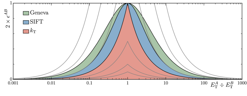
Figure 3: The factor $2\times\epsilon^{AB}$ is log-symmetric in the ratio $E_{\textrm{T}}^{A}/E_{\textrm{T}}^{B}$ of transverse energies, becoming small whenever candidate scales are hierarchically dissimilar. SIFT (blue) is compared against analogous behaviors for the Geneva (green) and $k_{\textrm{T}}$-family (red) algorithms, the latter at ($\,\beta\equiv E_{\textrm{T}}^{A}E_{\textrm{T}}^{B}/E_{0}^{2}\Rightarrow 1\,$). Grey contours illustrate scaling of the $k_{\textrm{T}}$ measures with a power $n=\pm 1$ of ($\,\beta\Rightarrow\nicefrac{{1}}{{10}},\,\nicefrac{{1}}{{5}},\,\nicefrac{{1}}{{2}},\,2,\,5,\,10\,$).

The indicated correspondence becomes increasingly exact as one approaches the collinear $(\Delta R^{2}\ll 1)$ and massless ($\Delta y\Rightarrow\Delta\eta$, $\xi\Rightarrow 1$) limits. The fact that $\cosh\Delta y$ is unbounded and has purely positive series coefficients, whereas $\cosh\Delta\phi$ is bounded and its terms are of alternating sign, implies that $\Delta\widetilde{R}^{2}$ is more sensitive to separations in rapidity than separations in azimuth.

The ratio ($\Delta\widetilde{R}^{2}\div\Delta R^{2}$) is explored graphically in FIG. 2 as a function of $\Delta\eta$ and $\Delta\phi$, for various values of ($m/p_{\textrm{T}}$). For purposes of illustration, deviations from ($\eta=0$) are applied symmetrically to the candidate object pair, and the quoted mass ratio applies equivalently to both objects. Black contours indicate unity, bisecting regions of neutral bias, which are colored in blue. Grey contours are spaced at increments of $0.1$ in the base-$10$ logarithm, and regions where SIFT exhibits enhancement (suppression) of clustering are colored green (red).

In the massless limit (lefthand panel) a near-symmetry persists under ($\Delta\eta\Leftrightarrow\Delta\phi$), with corrections from subleading terms as described previously. When $m$ approaches $p_{\textrm{T}}$ (center panel), the pseudo-rapidity versus azimuth symmetry is meaningfully broken at large $\Delta R$ and a strong aversion emerges to the clustering of massive states at small $\Delta R$. The latter effect dominates for highly non-relativistic objects (righthand panel), and extends to larger separations, such that the distinction between $\Delta\eta$ and $\Delta\phi$ is again washed out. SIFT binds objects approaching ($\Delta R\sim\pi$) significantly more tightly than the $k_{\textrm{T}}$ algorithms in this limit. Intuition for that crossover in sign can be garnered from leading terms in the multi-variate expansion shown following, as developed from Eqs. (10, 11, 31):

$$\Delta\widetilde{R}_{AB}^{2} \Rightarrow\Delta R_{AB}^{2}$$ (12)

$$+\Bigg{\{}1-\frac{\Delta R_{AB}^{2}}{2}\Bigg{\}}\times\Bigg{\{}\left(\frac{m_{A}}{p_{\textrm{T}}^{A}}\right)^{2}\!\!+\left(\frac{m_{B}}{p_{\textrm{T}}^{B}}\right)^{2}\Bigg{\}}+\cdots$$

We turn attention next to the denominator from Eq. (4), defining a new quantity $\epsilon^{AB}$ in conjunction with the transverse energy product factored out of $\Delta m_{AB}^{2}$.

$$\epsilon^{AB}\equiv\frac{E_{\textrm{T}}^{A}E_{\textrm{T}}^{B}}{(E_{\textrm{T}}^{A})^{2}+(E_{\textrm{T}}^{B})^{2}}=\left\{\left(\frac{E_{\textrm{T}}^{A}}{E_{\textrm{T}}^{B}}\right)+\left(\frac{E_{\textrm{T}}^{B}}{E_{\textrm{T}}^{A}}\right)\right\}^{-1}$$ (13)

This expression has a symmetry under the transformation $(\alpha\equiv E_{\textrm{T}}^{A}/E_{\textrm{T}}^{B}\Rightarrow\alpha^{-1})$. It is maximized at $\alpha=1$, where $(\epsilon^{AB}\Rightarrow\nicefrac{{1}}{{2}})$, and minimized at $\alpha=(0,+\infty)$, where $(\epsilon^{AB}\Rightarrow 0)$. The response is balanced by a change of variables $\Delta u=\ln\alpha$, i.e., $\alpha=e^{\Delta u}$, where the logarithm converts ratios into differences.

$$u \equiv\ln{\Big{(}E_{\textrm{T}}/{\rm[GeV]}\Big{)}}$$ (14)

$$\epsilon^{AB} ={\Big{(}e^{+\Delta u_{AB}}+e^{-\Delta u_{AB}}\Big{)}}^{-1}={\Big{(}2\cosh\Delta u_{AB}\Big{)}}^{-1}$$

Putting everything together, we arrive at a formulation of the measure from Eq. (4) that is expressed almost entirely in terms of coordinate differences of the rapidities, azimuths, and log-transverse energies, excepting the coefficients $\xi$ from Eq. (10), which depend on the ratios $m/p_{\textrm{T}}$. Of course, it is possible to adopt a reduction of the measure where $(\xi\Rightarrow 1)$ by fiat, which is equivalent to taking a massless limit in the fashion of JADE and Geneva, as described in Section III.

$$\delta_{AB} =\epsilon^{AB}\times\Delta\widetilde{R}_{AB}^{2}$$ (15)

$$=\frac{\cosh\Delta y_{AB}-\xi^{A}\xi^{B}\cos\Delta\phi_{AB}}{\cosh\Delta u_{AB}}$$

The scale-invariance of Eq. (15) is explicit, in two regards. By construction, there is no reference to an external angular cutoff $R_{0}$. In addition, the fact that transverse energies are referenced only via ratios, and never in absolute terms, is emergent. The measure is additionally observed to smoothly blend attributes of $k_{\textrm{T}}$ and anti-$k_{\textrm{T}}$ jet finding, insomuch as the former prioritizes clustering when one member of a pair is soft, the latter when one member of a pair is hard, and SIFT when the transverse energies are logarithmically disparate.

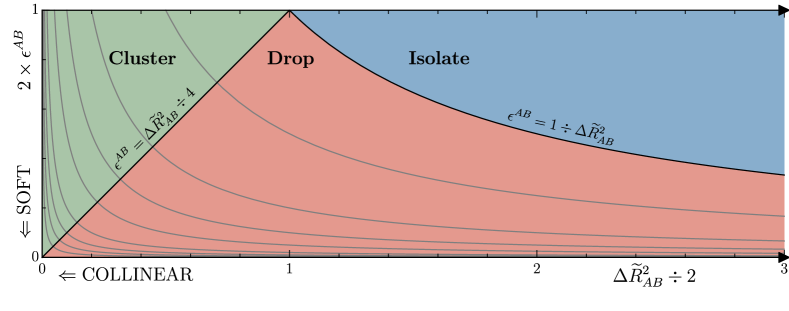
Figure 4: Phase diagram for the separation of object merging, filtering, and isolation responses.

This behavior is illustrated in FIG. 3, with $2\times\epsilon^{AB}$ plotted in blue as a function of ($\alpha\equiv E_{\textrm{T}}^{A}/E_{\textrm{T}}^{B}$). For comparison, the analogous momentum-dependent factor for Geneva from Eq. (6) is shown in green on the same axes, taking ($E\Rightarrow E_{\textrm{T}}$) and normalizing to unity at ($\alpha=1$). Like SIFT, Geneva is symmetric with respect to variation of the absolute event scale $\beta$. However, the extra cross term appearing in its denominator produces heavier tails when the scale ratio $\alpha$ is unbalanced. The cusped red region similarly represents the $k_{\textrm{T}}$ and anti-$k_{\textrm{T}}$ measures. Specifically, the following expression is proportional to Eq. (1) for ($n=\pm 1$) in the massless limit:

$$\delta_{AB}^{k_{\rm T},n}\,\mathrel{\vbox{ \offinterlineskip\halign{\hfil$#$\cr\propto\cr\kern 2.0pt\cr\sim\cr\kern-2.0pt\cr}}}\,{\left(\frac{E_{\textrm{T}}^{A}E_{\textrm{T}}^{B}}{E_{0}^{2}}\right)}^{\!\!n}\!\!\times{\rm min}\left[\frac{E_{\textrm{T}}^{A}}{E_{\textrm{T}}^{B}},\frac{E_{\textrm{T}}^{B}}{E_{\textrm{T}}^{A}}\right]$$ (16)

The selected normalization agrees with $2\times\epsilon^{AB}$ in the further limits ($\beta\equiv E_{\textrm{T}}^{A}E_{\textrm{T}}^{B}/E_{0}^{2}\Rightarrow 1$) and ($\alpha\Rightarrow 1$), where $E_{0}$ is an arbitrary constant reference energy. The distinction between $k_{\textrm{T}}$ and anti-$k_{\textrm{T}}$ clustering amounts to an enhancement versus suppression by the product (squared geometric mean) of transverse momenta. This is illustrated with the grey contours in FIG. 3, which rescale by $\beta=(\nicefrac{{1}}{{10}},\,\nicefrac{{1}}{{5}},\,\nicefrac{{1}}{{2}},\,2,\,5,\,10)$ from inner-lower to outer-upper for ($n=+1$), or in the reverse order for ($n=-1$). The $\beta$-invariant case ($n=0$) is also potentially of interest, but it is a new construction that is not to be confused with the Cambridge-Aachen algorithm, which has no energy dependence at all.

We conclude this section with a transformation that identifies the coordinate $u$ introduced in Eq. (14) as a sort of “dual” to the rapidity $y$ from Eq. (31). The log-transverse momentum $\ln(\,p_{\textrm{T}}\,/{\rm[GeV]})$ is similarly linked to pseudo-rapidity $\eta$ in the massless limit.

$$\Omega_{\pm} \equiv\phantom{\frac{1}{2}}\ln{\bigg{(}\frac{E\pm p_{z}}{{\rm[GeV]}}\bigg{)}}$$ (17)

$$\frac{\Omega_{+}+\hskip 2.0pt\Omega_{-}}{2} =\frac{1}{2}\ln{\bigg{(}\frac{E^{2}-p_{z}^{2}}{{\rm[GeV]}^{2}}\bigg{)}} \,=\,u$$

$$\frac{\Omega_{+}-\hskip 2.0pt\Omega_{-}}{2} =\frac{1}{2}\ln{\bigg{(}\frac{E+p_{z}}{E-p_{z}}\bigg{)}} \,=\,y$$

V Filtering, Isolation, and Halting

This section establishes the SIFT filtering and isolation criteria, which are used in conjunction to formulate a suitable halting condition for the non-exclusive clustering mode. Direct integration of a grooming stage effectively rejects stray radiation and pileup. SIFT’s behavior will be visualized with and without filtering in Section VII, and compared against each $k_{\textrm{T}}$-family algorithm in the presence of a soft “ghost” radiation background.

In conjunction, the two factorized terms in Eq. (15) ensure that clustering prioritizes the merger of object pairs that have a hierarchically soft member and/or that are geometrically collinear, mimicking fundamental poles in the matrix element for QCD showering. This behavior is illustrated by the “phase diagram” in FIG. 4, where the product of horizontal “$x$” and vertical “$y(x)$” coordinates on that plane is equal to $\delta_{AB}$. Grey “$y(x)=1/x$” contours trace constant values of the measure, equal to ($.002,\,.005,\,.01,\,.02,\,.05,\,.1,\,.2,\,.5$), with minimal values gathered toward the lower-left. As a consequence, SIFT successfully preserves mutually hard structures with tight angular adjacency, maintaining their resolution as distinct objects up to the final stages of clustering.

However, iterative application of the SIFT (or Geneva) measure does not offer an immediately apparent halting mechanism, and it will ultimately consume any presented objects into a single all-encompassing jet if left to run. These measures are additionally prone to sweeping up uncorrelated soft radiation onto highly-boosted partners at wide angular separation. The solution to both problems turns out to be related. For inspiration, we turn to the Soft Drop procedure, wherein a candidate jet is recursively declustered and the softer of separated constituents is discarded until the following criterion is satisfied:

$$\frac{\min\,(p_{\textrm{T}}^{A},p_{\textrm{T}}^{B})}{p_{\textrm{T}}^{A}+p_{\textrm{T}}^{B}}>z_{\rm cut}\left(\frac{\Delta R_{AB}}{R_{0}}\right)^{\beta}$$ (18)

The dimensionless $z_{\rm cut}$ coefficient is typically $\mathcal{O}(0.1)$. The exponent $\beta$ can vary for different applications, although we focus here on $\beta=2$. We first attempt to recast the elements of Eq. (18) into expressions with asymptotically similar behavior that adopt the vocabulary of Eq. (4). The factor $\Delta\widetilde{R}_{AB}^{2}$ can be carried over directly. Likewise, $\epsilon^{AB}$ behaves similarly to a minimized ratio of transverse energies, with the advantage of analyticity.

$$\epsilon^{AB} =\left\{\min\left(\frac{E_{\textrm{T}}^{A}}{E_{\textrm{T}}^{B}}\right)+\max\left(\frac{E_{\textrm{T}}^{A}}{E_{\textrm{T}}^{B}}\right)\right\}^{-1}$$

$$\simeq\left\{\max\left(\frac{E_{\textrm{T}}^{A}}{E_{\textrm{T}}^{B}}\right)\right\}^{-1}$$

$$=\min\left(\frac{E_{\textrm{T}}^{A}}{E_{\textrm{T}}^{B}}\right)\simeq\frac{\min(E_{\textrm{T}}^{A},E_{\textrm{T}}^{B})}{E_{\textrm{T}}^{A}+E_{\textrm{T}}^{B}}$$ (19)

Paired factors of $2$ previously emerged “naturally” in Eqs. (11, 14), and we group them here in a way that could be interpreted as setting “$z_{\rm cut}=\nicefrac{{1}}{{4}}$” in the context of a large-radius $(R_{0}=1)$ jet. Putting all of this together, the suggested analog to Eq. (18) is shown following.

$$\textrm{Cluster:}\hskip 12.0pt\frac{\Delta\widetilde{R}_{AB}^{2}}{2}<\big{\{}\left(2\,\epsilon^{AB}\right)\leq 1\big{\}}$$ (20)

An important distinction from conventional usage is that this protocol is to be applied during the initial clustering cycle itself, at the point of each candidate merger. This is similar in spirit to Recursive Soft Drop [16].

Intuition may be garnered by turning again to FIG. 4, where clustering consistent with the Eq. (20) prescription is observed to occur only in the upper-left (green) region of the phase diagram, above the “$y(x)=x$” diagonal cross-cutting contours of the measure. The upper bound on $(2\,\epsilon^{AB})$ precludes clustering if $(\Delta\widetilde{R}_{AB}\geq\sqrt{2})$. However, this angular threshold is dynamic, and the capturable cone diminishes in area with increasing imbalance of the transverse scales. This condition may be recast into a limit on the clustering measure from Eq. (15).

$$\textrm{Cluster:}\hskip 12.0pt\delta_{AB}<\big{\{}\left(2\,\epsilon^{AB}\right)^{2}\leq 1\big{\}}$$ (21)

The question now is what becomes of those objects rejected by the Eq. (21) filter. Specifically, are they discarded, or are they classified for retention as isolated final-state jets? One possible solution is to simply determine this based on the magnitude of the transverse energy, but that runs somewhat counter to current objectives. Seeking a simple scale-invariant criterion for selecting between isolation and rejection, we observe that there are distinct two ways in which Eq. (20) may fail. Namely, the angular opening may be too wide, and/or the transverse scales may be too hierarchically separated. This is illustrated again by FIG. 4, wherein one may exit the clustering region (green) by moving rightward (wider angular separation) or downward (more scale disparity).

If the former cause is dominant, e.g., if $(\Delta\widetilde{R}_{AB}^{2}\gg 1)$ and $(\epsilon^{AB}\sim 1)$ such that both members are on equal footing and $(\delta_{AB}\gg 1)$, then collective isolation as a pair of distinct final states is appropriate. Conversely, if the latter cause primarily applies, e.g., if $(\epsilon^{AB}\ll 1)$ and $(\Delta\widetilde{R}_{AB}^{2}\sim 1)$ such that $(\delta_{AB}\ll 1)$, then the pertinent action is to asymmetrically set aside just the softer candidate. These scenarios may be quantitatively distinguished in a manner that generates a balance with and continuation of Eq. (20), as follows.

Drop: $$\hskip 3.0pt\big{\{}\left(2\,\epsilon^{AB}\right)\leq 1\big{\}} \leq\frac{\Delta\widetilde{R}_{AB}^{2}}{2}<\big{\{}1\leq\left(2\,\epsilon^{AB}\right)^{-1}\big{\}}$$

Isolate: $$\hskip 3.0pt\big{\{}1\leq\left(2\,\epsilon^{AB}\right)^{-1}\big{\}} \leq\frac{\Delta\widetilde{R}_{AB}^{2}}{2}$$ (22)

Each criterion may also be recast in terms of the clustering measure, with isolation always and only indicated against an absolute reference value ($1$) of the SIFT measure $\delta_{AB}$ that heralds a substantial mass-gap. Observe that the onset of object isolation necessarily culminates in global algorithmic halting since all residual pairings must correspond to larger values of $\delta_{AB}$.

Drop: $$\hskip 8.0pt\big{\{}\left(2\,\epsilon^{AB}\right)^{2}\leq 1\big{\}} \leq\delta_{AB}<\big{\{}1\big{\}}$$

Isolate: $$\hskip 8.0pt\big{\{}1\big{\}} \leq\delta_{AB}$$ (23)

FIG. 4 again provides visual intuition, where isolation occurs in the upper-right (blue) regions for values of the measure above unity, and soft wide radiation is dropped in the lower-central (red) regions. The clustering and isolation regions are fully separated from each other, making contact only at the zero-area “triple point” with ($2\,\epsilon^{AB}=1$, $\Delta\widetilde{R}_{AB}^{2}/2=1$). We will provide additional support from simulation for triggering isolation at a fixed $\mathcal{O}(1)$ value of the measure in Section IX.

Note that non-relativistic or beam-like objects at very large rapidity that approach the ($p_{\textrm{T}}\Rightarrow 0$, $m\neq 0$) limit will never cluster, since vanishing of the lever arm ($\xi=0$) in Eq. (10) implies via Eq. (11) that ($\Delta\widetilde{R}_{AB}^{2}/2\geq 1$). Also, objects of equivalent transverse energy with angular separation $(\Delta\widetilde{R}_{AB}\geq\sqrt{2})$ will always be marked for isolation, although this radius is again dynamic. The phase gap between clustering and isolation opens up further when scales are mismatched, and the effective angular square-separation exceeds its traditional counterpart as mass is accumulated during clustering (cf. Eq. 12).

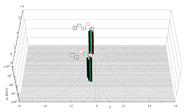
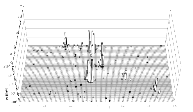
Figure 5: Upper: A simulated LHC scattering event with $\sqrt{s}=14$ TeV is visualized at the partonic level. Top quark pair production $pp\to t\bar{t}$ (red, red) is followed by the decays $t\to W^{+}b$ (green, black) and $W^{+}\to u\,\bar{d}$ (black, black), plus conjugates. A transverse boost of $p_{\textrm{T}}\simeq 800$ GeV for each top quark produces narrow collimation of decay products. Lower: Generator-level radiation deposits resulting from showering, hadronization, and decay of the partonic event appearing in the upper frame.

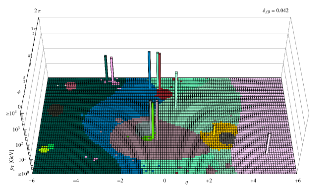
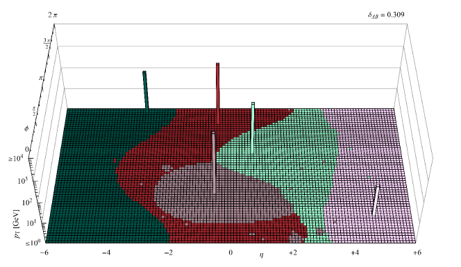
Figure 6: Frames representing sequential clustering of the FIG. 5 event using the exclusive $N_{\rm exc}=1$ SIFT algorithm without the associated filtering or isolation criteria (cf. FIG. 10 for non-exclusive clustering with both criteria enabled). Upper: Mutually hard prongs with narrow angular separation remain unmerged up to the final stages of clustering. However, hard objects are likely to sweep up soft radiation at wide angles. Lower: An image of the initial pair production is reconstructed just prior to termination. In the absence of a supplementary halting criterion these structures will subsequently merge to completion, accompanied by a large discontinuity in the measure $\delta_{AB}$.

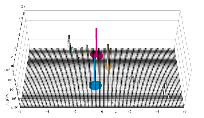
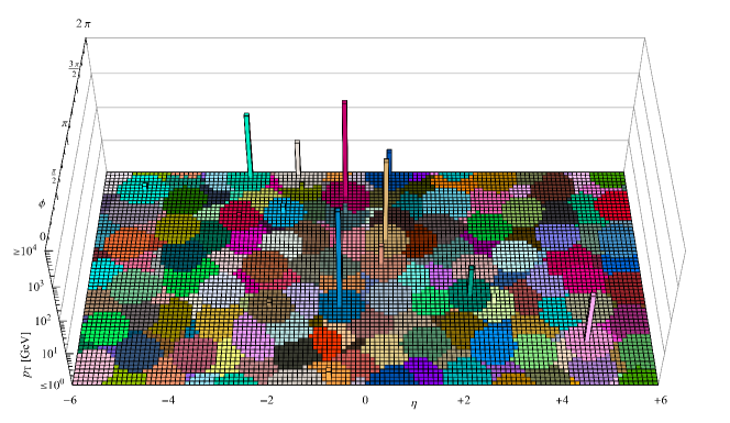
Figure 7: Frames representing sequential clustering of the FIG. 5 event using the anti-$k_{\textrm{T}}$ algorithm. Upper: Priority is given to the hardest radiation, which immediately captures surrounding territory. Hard substructure at angular scales smaller than the clustering radius will be washed out rapidly. Lower: The final state is characterized by regular jet shapes with uniform expected areas.

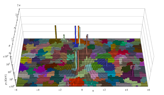
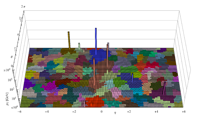
Figure 8: Frames representing sequential clustering of the FIG. 5 event using the $k_{\textrm{T}}$ algorithm. Upper: Priority is given to the softest radiation, resulting in the growth of dispersed catchments having a correlation length that increases in time. Mutually hard substructures are preserved until the last stages of clustering. Lower: The final state is characterized by irregular jet shapes with unpredictable areas.

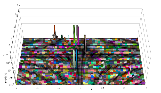
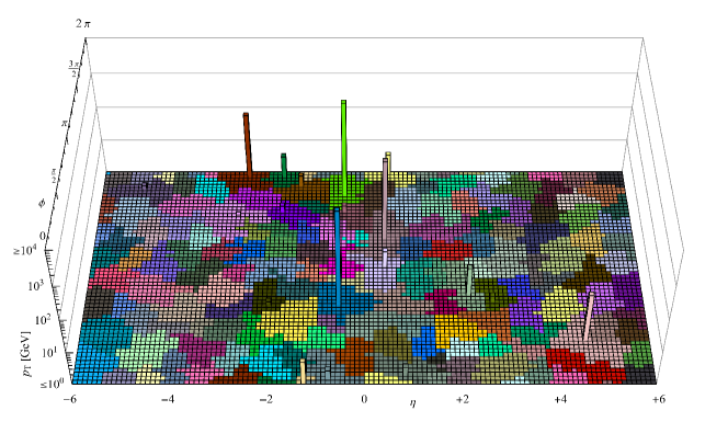
Figure 9: Frames representing sequential clustering of the FIG. 5 event using the Cambridge-Aachen algorithm. Upper: Priority is given only the angular proximity, without reference to the momentum scale. Substructure is preserved only until the grain size eclipses its angular scale. Lower: The final state is characterized by irregular jet shapes with unpredictable areas.

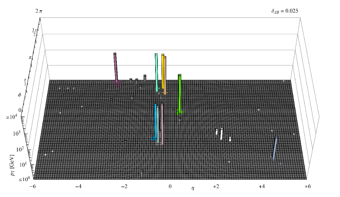
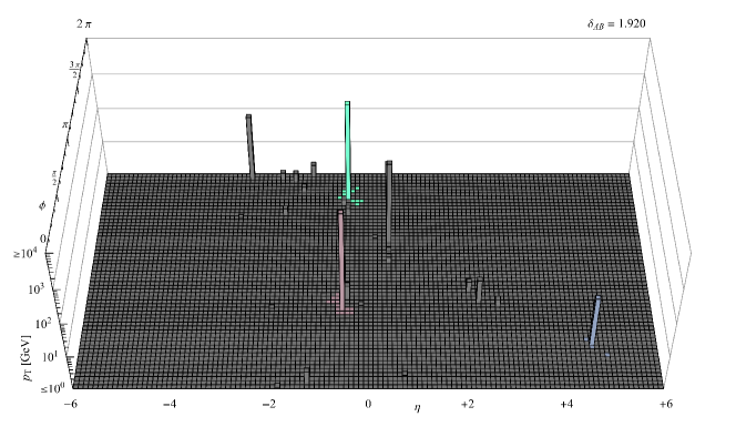
Figure 10: Frames representing sequential clustering of the FIG. 5 event using the SIFT algorithm with the application of filtering and isolation criteria. Upper: Initial activity is dominated by the rejection of soft-wide radiation that is paired with a hard prong by the measure but fails the filtering criterion. Mutually hard substructures are resolved without contamination from stray radiation. Lower: The isolation criterion triggers halting before distinct objects associated with the initial pair production would be merged.

VI The $\boldsymbol{N}$-Subjet Tree

This section concludes development of the SIFT algorithm by formalizing the concept of an $N$-subjet tree. This data structure records the clustering history of each isolated final-state object from $N$ prongs down to $1$, along with the associated value of the measure at each merger.

Final-state jets defined according to the global halting condition outlined in Section V may still bundle multiple hard structured prongs, since isolation requires a minimal separation of $(\Delta\widetilde{R}_{AB}\geq\sqrt{2})$. Within each quarantined partition, SIFT reverts to its natural form, as an exclusive clustering algorithm. So, for example, it might be that reconstruction of a doubly-hadronic $t\bar{t}$ event would isolate the pair of top-quark remnants, but merge each bottom with products from the associated $W$. This is a favorable outcome, amounting to the identification of variable large-radius jets. But, the question of how to identify and recover the optimal partition of each such object into $N$ subjets remains.

One could consider formulating a local halting condition that would block the further assimilation of hard prongs within each large-radius jet once some threshold were met. However, such objects are only defined in our prescription after having merged to exhaustion. More precisely, a number of candidate large-radius jets may accumulate objects in parallel as clustering progresses, and each will have secured a unique “$N=1$” configuration at the moment of its isolation.

As such, the only available course of action appears to be proceeding with these mergers, even potentially in the presence of substructure. However, the fact that the SIFT measure tends to preserve mutually hard features until the final stages of clustering suggests that suitable proxies for the partonic event axes may be generated automatically as a product of this sequential transition through all possible subjet counts, especially during the last few mergers. We refer to the superposed ensemble of projections onto ($N=\ldots,\,3,\,2,\,1$) prongs, i.e., the history of residually distinct four-vectors at each level of the clustering flow, as an $N$-subjet tree.

In fact, it seems that interrupting the final stages of clustering would amount to a substantial information forfeiture. Specifically, the merger of axis candidates that are not collinear or relatively soft imprints a sharp discontinuity on the measure, which operates in this context like a mass-drop tagger [17] to flag the presence of substructure. Additionally, the described procedure generates a basis of groomed axes that are directly suitable for the computation of observables such as $N$-subjettiness. In this sense, the best way to establish that a pair of constituents within a large-radius jet should be kept apart may be to go ahead and join them, yet to remember what has been joined and at which value of $\delta_{AB}$.

In contrast to conventional methods for substructure recovery that involve de- and re-clustering according to a variety of disjoint prescriptions, the finding of $N$-subjet trees representing a compound scattering event occurs in conjunction with the filtering of stray radiation and generation of substructure observables during a single unified operational phase. The performance of this approach for kinematic reconstruction and tagging hard event prongs will be comparatively assessed in Sections VIII and IX.

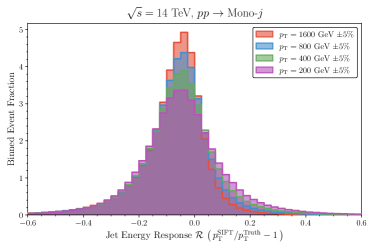
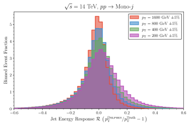
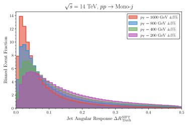
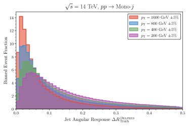
Figure 11: Top: Distribution $\mathcal{R}^{A}_{B}$ of reconstructed jet energy responses with detector effects relative to the partonic truth level at various transverse boosts. Bottom: Distribution $\Delta R^{\,A}_{\,B}$ of reconstructed jet angular responses with detector effects relative to the partonic truth level at various transverse boosts. Lefthand panels represent the leading filtered and isolated SIFT jet, while righthand panels represent the leading ($R_{0}=1$) large-radius Soft Drop jet reported by Delphes. No calibration of jet energy scales is attempted for either category.

$p_{\textrm{T}}^{{\rm GeV}\pm 5\%}$	$\langle\,\mathcal{R}^{\rm\,SIFT}_{\rm\,Truth}\,\rangle$	$\sigma^{\rm SIFT}_{\mathcal{R}}$	$\langle\,\mathcal{R}^{\rm\,\textsc{Delphes}}_{\rm\,Truth}\,\rangle$	$\sigma^{\rm\textsc{Delphes}}_{\mathcal{R}}$	$\langle\,\Delta R^{\rm\,SIFT}_{\rm\,Truth}\,\rangle$	$\sigma^{\rm SIFT}_{\!\Delta R}$	$\langle\,\Delta R^{\rm\,\textsc{Delphes}}_{\rm\,Truth}\,\rangle$	$\sigma^{\rm\textsc{Delphes}}_{\!\Delta R}$
100	$-0.009$	0.17	$+0.087$	0.17	0.17	0.12	0.17	0.12
200	$-0.046$	0.16	$+0.026$	0.16	0.15	0.12	0.15	0.12
400	$-0.059$	0.15	$-0.002$	0.15	0.13	0.11	0.13	0.11
800	$-0.071$	0.14	$-0.024$	0.14	0.10	0.10	0.10	0.10
1600	$-0.081$	0.13	$-0.042$	0.13	0.08	0.09	0.08	0.09
3200	$-0.089$	0.12	$-0.058$	0.12	0.05	0.06	0.05	0.06

Table 1: Detector-level jet energy responses $\mathcal{R}^{A}_{B}$ and angular responses $\Delta R^{A}_{B}$ with associated resolutions $\sigma_{\mathcal{R}}$ and $\sigma_{\!\Delta R}$.

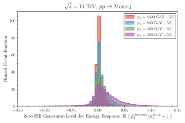
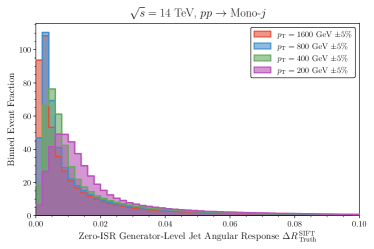
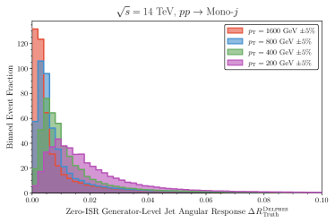
Figure 12: Top: Distribution $\mathcal{R}^{A}_{B}$ of reconstructed jet energy responses, at generator level and without initial-state radiation, relative to the partonic truth level at various transverse boosts. Bottom: Distribution $\Delta R^{\,A}_{\,B}$ of reconstructed jet angular responses, at generator level and without initial-state radiation, relative to the partonic truth level at various transverse boosts. Lefthand panels represent the leading filtered and isolated SIFT jet, while righthand panels represent the leading ($R_{0}=1$) large-radius Soft Drop jet reported by Delphes. No calibration of jet energy scales is attempted for either category.

$p_{\textrm{T}}^{{\rm GeV}\pm 5\%}$	$\langle\,\mathcal{R}^{\rm\,SIFT}_{\rm\,Truth}\,\rangle$	$\sigma^{\rm SIFT}_{\mathcal{R}}$	$\langle\,\mathcal{R}^{\rm\,\textsc{Delphes}}_{\rm\,Truth}\,\rangle$	$\sigma^{\rm\textsc{Delphes}}_{\mathcal{R}}$	$\langle\,\Delta R^{\rm\,SIFT}_{\rm\,Truth}\,\rangle$	$\sigma^{\rm SIFT}_{\!\Delta R}$	$\langle\,\Delta R^{\rm\,\textsc{Delphes}}_{\rm\,Truth}\,\rangle$	$\sigma^{\rm\textsc{Delphes}}_{\!\Delta R}$
100	$-0.059$	0.054	$+0.034$	0.052	0.038	0.052	0.043	0.049
200	$-0.052$	0.049	$+0.013$	0.040	0.030	0.050	0.030	0.050
400	$-0.045$	0.045	$+0.004$	0.033	0.025	0.047	0.022	0.047
800	$-0.040$	0.042	$-0.001$	0.031	0.022	0.045	0.018	0.046
1600	$-0.035$	0.039	$-0.003$	0.029	0.018	0.040	0.015	0.042
3200	$-0.031$	0.035	$-0.004$	0.025	0.015	0.032	0.011	0.033

Table 2: Zero-ISR generator-level jet energy responses $\mathcal{R}^{A}_{B}$ and angular responses $\Delta R^{A}_{B}$ with associated resolutions $\sigma_{\mathcal{R}}$ and $\sigma_{\!\Delta R}$.

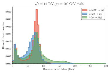
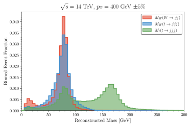
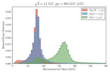
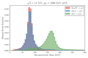
Figure 13: Distribution of $W$-boson and top quark masses for di, and tri-jet samples reconstructed with SIFT at various transverse boosts.

VII Comparison of Algorithms

This section provides a visual comparison of merging priorities and final states for the SIFT and $k_{\textrm{T}}$-family algorithms. The images presented here are still frames extracted from full-motion video simulations of each clustering sequence. These films are provided as ancillary files with the source package for this paper on the arXiv and may also be viewed on YouTube [18]. Frames are generated for every 25th clustering action, as well as each of the initial and final 25 actions. The Mathematica notebook used to generate these films is described in Appendix B, and maintained with the AEACuS [19] package on GitHub.

The visualized event comes from a simulation in MadGraph/MadEvent [20] of top quark pair production at the 14 TeV LHC with fully hadronic decays. The scalar sum $H_{\rm T}$ of transverse momentum is approximately 1.6 TeV at the partonic level. This large boost results in narrow collimation of the three hard prongs (quarks) on either side of the event, as depicted in the the upper frame of FIG. 5. In-plane axes represent the pseudo-rapidity $\eta$ and azimuth $\phi$, with a cell width ($\Delta R\simeq 0.1$) approximating the resolution of a modern hadronic calorimeter. The height of each block is proportional to the log-transverse momentum $\log_{10}(\,p_{\textrm{T}}\,/{\rm[GeV]})$ it contains.

The event is passed through through Pythia8 [21] for showering and hadronization, and through Delphes [22] for fast detector simulation. Detector effects are bypassed in the current context, which starts with unclustered generator-level (Pythia8) jets and non-isolated photons/leptons extracted from the Delphes event record by AEACuS, but they will be included for most of the analysis in Sections VIII and IX. This initial state is depicted in the lower frame of FIG. 5, which exhibits two dense clusters of radiation that are clearly associated with the partonic event, as well as several offset deposits having less immediate origins in the underlying event or initial state. Prior to clustering, a sheet of ultra-soft ghost radiation is distributed across the angular field in order to highlight differences between the catchment area [23] of each algorithm.

We begin with an example of exclusive ($N_{\rm exc}=1$) clustering ordered by the SIFT measure from Eq. 4, but without application of the filtering and isolation criteria described in Section V. Film A clearly exhibits both of the previously identified pathologies, opening with a sweep of soft-wide radiation by harder partners (as visualized with regions of matching coloration) and closing with the contraction of hard-wide structures into a single surviving object. However, the described success is manifest in between, vis-à-vis mutual preservation of narrowly bundled hard prongs until the end stages of clustering. In particular, the upper frame of FIG. 6 features a pair of triplets at ($\delta_{AB}\simeq 0.04$) that fairly approximate their collinear antecedents despite bearing wide catchments. Subsequently, this substructure collapses into an image of the original pair production, as depicted at ($\delta_{AB}\simeq 0.3$) in the lower frame of FIG. 6. Nothing further occurs until ($\delta_{AB}\gtrsim 1.0$), beyond which residual structures begin to merge and migrate in unphysical ways.

For comparison, we process the same event using the anti-$k_{\textrm{T}}$ algorithm at ($R_{0}=0.5$). Film B shows how early activity is dominated by the hardest radiative seeds, which promptly capture all available territory up to the stipulated radial boundary. In particular, any substructure that is narrower than $R_{0}$ will be rapidly erased, as illustrated in the upper frame of FIG. 7. The subsequent stages of clustering are of lesser interest, being progressively occupied with softer seeds gathering up yet softer unclaimed scraps. At termination, the lower frame of FIG. 7 exhibits the regular cone shapes with uniform catchment areas that are a hallmark of anti-$k_{\textrm{T}}$. This property is linked to the anchoring of new cones on hard prongs that are less vulnerable to angular drift. It is favored by experimentalists for facilitating calibration of jet energy scales and subtraction of soft pileup radiation.

Proceeding, we repeat the prior exercise using the $k_{\textrm{T}}$ algorithm at ($R_{0}=0.5$). In contrast to anti-$k_{\textrm{T}}$, clustering is driven here by the softest seeds. Film C demonstrates the emergence of a fine grain structure in the association pattern of objects from adjacent regions that grows in size as the algorithm progresses. Unlike SIFT, which preferentially binds soft radiation to a hard partner, mutually soft objects without a strong physical correlation are likely to pair in this case. Since summing geometrically adjacent partners tends increase $p_{\textrm{T}}$, merged objects become less immediately attractive to the measure. As a result, activity is dispersed widely across the plane, and attention jumps rapidly from one location to the next. However, the combination of mutually hard prongs is actively deferred, which causes collimated substructures to be preserved, as shown in the upper frame of FIG. 8. In contrast to SIFT, this hardness criterion is absolute, rather than relative. Ultimately, structures more adjacent than the fixed angular cutoff $R_{0}$ will still be absorbed. Jet centers are likely to drift substantially, and associated catchment shapes are thus highly irregular, as shown in the lower frame of FIG. 8.

Similarly, we also cluster using the Cambridge Aachen algorithm at ($R_{0}=0.5$). Pairings are driven here solely by angular proximity, and Film D shows an associated growth of grain size that is like that of the $k_{\textrm{T}}$ algorithm. The banded sequencing is simply an artifact of the way we disperse ghost jets, randomizing $p_{\textrm{T}}$ but regularizing placement on the grid. In contrast, mutually hard substructures are not specifically protected and will last only until the correlation length catches up to their separation, as shown in the upper frame of FIG. 9. As before, the angular cutoff $R_{0}$ limits resolution of structure. Likewise, jet drift leads to irregular catchment shapes, as shown in the lower frame of FIG. 9.

We conclude this section with a reapplication of the SIFT algorithm, enabling the filtering and isolation criteria from Section V. Film E demonstrates that the soft ghost radiation is still targeted first, but it is now efficiently discarded (as visualized with dark grey) rather than clustered, suggesting resiliency to soft pileup. Hard substructures are resolved without accumulating stray radiation, as shown in the upper frame of FIG. 10. This helps to stabilize reconstructed jet kinematics relative to the parton-level event. Objects decayed and showered from the pair of opposite-hemisphere top quarks are fully isolated from each other in the final state, as shown in the lower frame of FIG. 10. Each such object selectively associates constituents within a “fuzzy” scale-dependent catchment boundary. Nevertheless, it may still be possible to establish an “effective” jet radius by integrating the pileup distribution function up to the maximal radius $(\Delta\widetilde{R}_{AB}<\sqrt{2})$. In any case, the traditional approach to pileup subtraction has been somewhat superseded by the emergence of techniques for event-by-event, and per-particle pileup estimation like PUPPI [24].

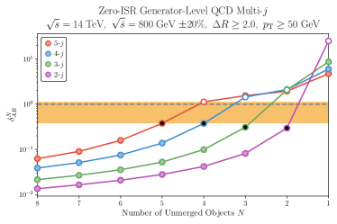
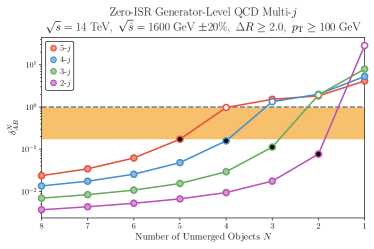
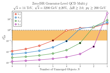
Figure 14: Evolution of the measure $\delta^{N}_{AB}$ as a function of the number $N$ of unmerged objects for QCD multi-jet production at various values of $\sqrt{\hat{s}}$. Partons have an angular separation ($\Delta R\geq 2.0$) and the $p_{\textrm{T}}$ threshold is stepped in proportion to $\sqrt{\hat{s}}$. Initial-state radiation is suppressed and analysis is at generator level. The orange band indicates the interval where all samples have merged to the point of their natural partonic count (white) but not beyond (black). The grey dashed line marks the isolation threshold at ($\delta_{AB}=1$).

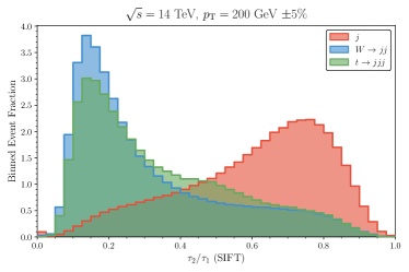
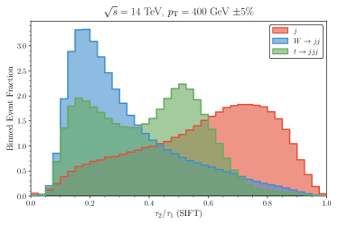
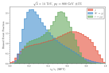
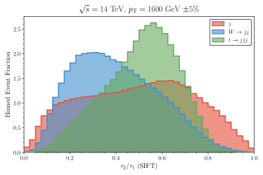
Figure 15: Distribution of $\tau_{2}/\tau_{1}$ computed with SIFT axes for mono-, di-, and tri-jet samples at various transverse boosts.

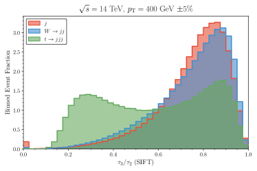
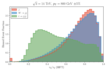
Figure 16: Distribution of $\tau_{3}/\tau_{2}$ computed with SIFT axes for mono-, di-, and tri-jet samples at various transverse boosts.

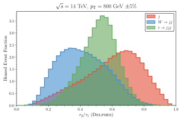
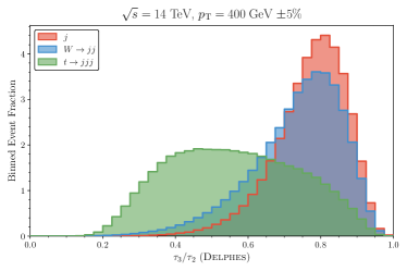
Figure 17: Reference distributions of $\tau_{2}/\tau_{1}$ and $\tau_{3}/\tau_{2}$ computed by Delphes at various transverse boosts.

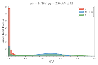
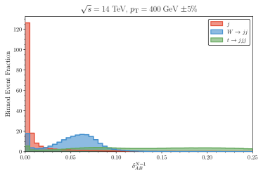
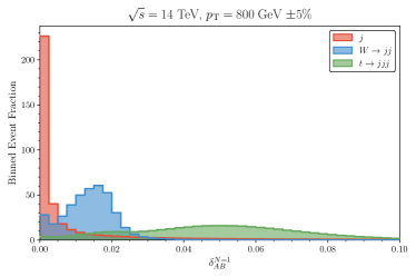
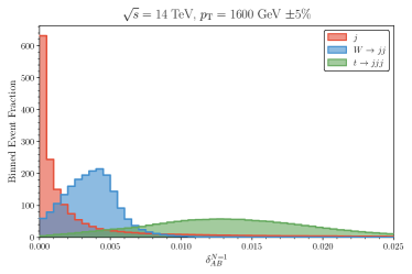
Figure 18: Distribution of $\delta_{AB}$ at the $N=1$ stage of clustering with SIFT for mono-, di-, and tri-jet samples at various transverse boosts.

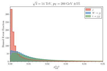
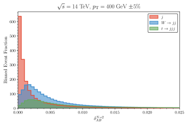
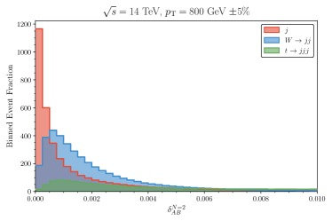
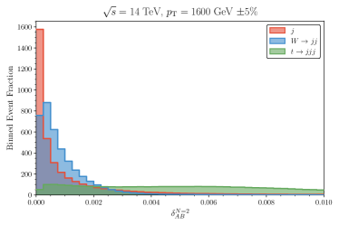
Figure 19: Distribution of $\delta_{AB}$ at the $N=2$ stage of clustering with SIFT for mono-, di-, and tri-jet samples at various transverse boosts.

$p_{\textrm{T}}^{{\rm GeV}\pm 5\%}$	$\tau_{\textsc{Delphes}}^{N+1/N}$	$\tau_{\rm SIFT}^{N+1/N}$	$\delta_{AB}^{N}$	$\delta+\tau$
100	0.62	0.68	0.69	0.70
200	0.91	0.86	0.88	0.89
400	0.89	0.85	0.91	0.92
800	0.82	0.79	0.92	0.93
1600	0.77	0.74	0.91	0.92
3200	0.78	0.76	0.88	0.90

Table 3: Area under curve ROC scores for discrimination of resonances with hard 1- and 2-prong substructure using a BDT trained on various sets of event observables.

$p_{\textrm{T}}^{{\rm GeV}\pm 5\%}$	$\tau_{\textsc{Delphes}}^{N+1/N}$	$\tau_{\rm SIFT}^{N+1/N}$	$\delta_{AB}^{N}$	$\delta+\tau$
100	0.61	0.61	0.63	0.65
200	0.63	0.60	0.71	0.72
400	0.82	0.74	0.90	0.90
800	0.85	0.80	0.94	0.95
1600	0.77	0.77	0.97	0.97
3200	0.77	0.79	0.98	0.99

Table 4: Area under curve ROC scores for discrimination of resonances with hard 2- and 3-prong substructure using a BDT trained on various sets of event observables.

$p_{\textrm{T}}^{{\rm GeV}\pm 5\%}$	$\tau_{\textsc{Delphes}}^{N+1/N}$	$\tau_{\rm SIFT}^{N+1/N}$	$\delta_{AB}^{N}$	$\delta+\tau$
100	0.70	0.75	0.77	0.77
200	0.86	0.87	0.90	0.90
400	0.93	0.91	0.95	0.96
800	0.91	0.89	0.96	0.96
1600	0.84	0.83	0.94	0.95
3200	0.76	0.78	0.91	0.92

Table 5: Area under curve ROC scores for discrimination of resonances with hard 3- and 1-prong substructure using a BDT trained on various sets of event observables.

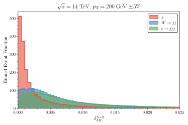
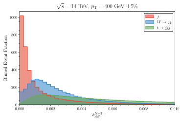
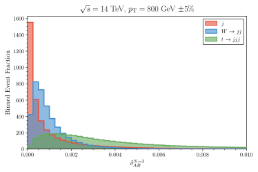
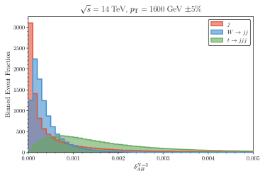
Figure 20: Distribution of $\delta_{AB}$ at the $N=3$ stage of clustering with SIFT for mono-, di-, and tri-jet samples at various transverse boosts.

VIII Resolution and Reconstruction

This section characterizes SIFT’s angular and energetic response functions for the resolution of hard mono-jets and tests the reconstruction of collimated di- and tri-jet systems associated with a massive resonance. The best performance is achieved for large transverse boosts.

We generate Monte Carlo collider data modeling the $\sqrt{s}=14$ TeV LHC using MadGraph/MadEvent, Pythia8, and Delphes as before. Clean ($N=1,2,3$) prong samples are obtained by simulating the processes ($pp\Rightarrow jZ\Rightarrow j+\nu\bar{\nu}$), ($pp\Rightarrow W^{\pm}Z\Rightarrow jj+\nu\bar{\nu}$), and ($pp\Rightarrow tW^{-}\Rightarrow jjj+\bar{\nu}\ell^{-}$) plus conjugate, respectively. In the latter case, an angular isolation cone with ($\Delta R=0.5$) is placed around the visible lepton. Hard partonic objects are required to carry a minimal transverse momentum ($p_{\textrm{T}}\geq 25$ GeV) and be inside ($|\eta|<=3.0$). No restrictions are placed on the angular separation of decay products. Jets consist of gluons and/or light first-generation quarks ($u,\,d$), as well as $b$-quarks where required by a third-generation process. In order to represent a wide range of event scales, we tranche in the transverse momentum (vector sum magnitude) of the hadronic system, considering six log-spaced intervals $p_{\textrm{T}}=(\,100,\,200,\,400,\,800,\,1600,\,3200\,)$ GeV $\pm 5\%$ and giving attention primarily to the inner four.

Clustering is disabled at the detector simulation level by setting the jet radius $R_{0}$ and aggregate $p_{\textrm{T}}$ threshold to very small values. We retain the default Delphes efficiencies for tracks and calorimeter deposits (including $p_{\textrm{T}}$ thresholds on low-level detector objects), along with cell specifications and smearing (resolution) effects in the latter case. Jet energy scale corrections are turned off (set to $1.0$) since these are calibrated strictly for application to fully reconstructed (clustered) objects. For purposes of comparison and validation, we also extract information from Delphes regarding the leading large-radius jet ($R_{0}=1$), which is processed by trimming [25], pruning [26], and applying Soft-Drop.

Event analysis (including clustering) and computation of observables are implemented with AEACuS (cf. Appendix B). We begin by pre-clustering detector-level objects with anti-$k_{\textrm{T}}$ at ($R_{0}=0.01$) to roughly mimic a characteristic track-assisted calorimeter resolution at the LHC. The isolation and filtering criteria described in Section V are then used in conjunction to select the subset of detector-level object candidates retained for analysis. Specifically, our procedure is equivalent to keeping members gathered by the hardest isolated $N$-subjet tree that survive filtering all the way down to the final merger. All histograms are generated with RHADAManTHUS [19], using MatPlotLib [27] on the back end.

We begin by evaluating the fidelity of the variable large-radius SIFT jet’s directional and scale reconstruction in the context of the mono-jet sample. Respectively, the upper-left and lower-left panels of FIG. 11 show distributions of the energy response $\mathcal{R}^{A}_{B}\equiv(\,p_{\textrm{T}}^{A}/p_{\textrm{T}}^{B}-1\,)$ and angular response $\Delta R^{A}_{B}$ relative to the original truth-level (MadGraph) partonic jet at various transverse boosts. The corresponding right-hand panels feature the same two distributions for the leading large-radius jet identified by Delphes. The vanishing tail of events for which the SIFT or Delphes jet fails ($\Delta R\leq 0.5$) relative to the partonic sum are vetoed here and throughout.

Central values and associated widths (standard deviations) are provided for the $\mathcal{R}^{A}_{B}$ and $\Delta R^{A}_{B}$ in TABLE 1. The SIFT variable-radius jet energy response is very regular, systematically under-estimating the momentum of hard objects by about 6%. The Delphes jet energy response shows more drift, transitioning from positive values for soft objects to negative values for hard objects. Widths of the two distributions are indistinguishable, with fluctuations amounting to about 15% in both cases, narrowing slightly at larger boosts. It is anticipated from these observations that an energy calibration of SIFT jets would be relatively straightforward, using standard techniques. Angular performance of the two methodologies is identical, with typical offsets and deviations both near one-tenth of a radian (but less for hard objects and more for soft objects).

For comparison, we repeat this analysis in FIG. 12 and TABLE 2, using generator-level (Pythia8) objects without detector effects and suppressing the emission of initial-state radiation. The distributions are substantially narrower in all cases, with widths around a half or a third of the prior reference values. The energy response is affected by both idealizations, but more so by the elimination of detector effects, whereas the angular response is improved primarily by the elimination of initial-state radiation. The most distinctive difference between the SIFT and large-radius Delphes jets at this level is that the former is bounded from above by the partonic $p_{\textrm{T}}$, while the latter commonly exceeds it. The observed momentum excess is attributable to the capture of radiation from the underlying event. However, SIFT’s filtering stage is apparently more adept at rejecting this contaminant, producing a reflection in the tail orientation that is reminiscent of various approaches to grooming.

Proceeding, we turn to attention the reconstruction of $W$-boson and top quark mass resonances, as visualized in FIG. 13 at each of the four central simulated $p_{\textrm{T}}$ ranges. $M_{W}$ and $M_{t}$ are respectively recovered from di- and tri-jet samples, by summing and squaring residual four-vector components after filtering. A second $W$ reconstruction is obtained from decays of a $t$ by optimizing the combinatoric selection of two prongs from the ($N=3$) clustering flow. An excess near $M_{W}\simeq 80$ GeV is apparent for $p_{\textrm{T}}\geq 200$ GeV, although the top quark remains unresolved by the leading SIFT jet at low boost, since the associated bottom is likely to be separately isolated. The top-quark bump is clearly visible for $p_{\textrm{T}}\geq 400$ GeV, though its centroid falls somewhat to the left of $M_{t}\simeq 175$ GeV. The plotted distributions narrow at higher boost, and substantially sharper peaks are observed for $p_{\textrm{T}}\geq 800$ GeV. The systematic under-estimation of mass is consistent with effects observed previously in the jet energy response, and it is similarly expected to be improvable with a suitable calibration.

IX Structure Tagging

This section describes applications of the SIFT algorithm related to structure and substructure tagging, including discrimination of events with varying partonic multiplicities, $N$-subjettiness axis-finding, and identification of heavy resonances. We comparatively assess SIFT’s performance on Monte Carlo collider data against standard approaches, and quantify its discriminating power with the aid of a Boosted Decision Tree (BDT).

Our first objective will be characterizing distinctive features in the evolution of the SIFT measure $\delta_{AB}$ for events with different numbers of hard prongs. We proceed by simulating pure QCD multi-jets representing LHC production of ($N=2\text{--}5$) gluons and/or light first-generation quarks ($u,\,d$). Samples are generated at various partonic center-of-momentum energies, taking $\sqrt{\hat{s}}=(\,100,\,200,\,400,\,800,\,1600,\,3200\,)$ GeV $\pm 20\%$. In order to ensure that splittings are hard and wide (corresponding to a number of non-overlapping large-radius jets with more or less commensurate scales), we require ($\,p_{\textrm{T}}\geq\sqrt{\hat{s}}\div 16\,$) and ($\,\Delta R\geq 2.0\,$). We also suppress initial-state radiation so that consistent partonic multiplicities can be achieved, and return to the use of generator-level (Pythia8) objects. Other selections and procedures are carried forward.

In contrast to the examples in Section VIII, the relevant showering products of these non-resonant systems are not expected to be captured within a single variable large-radius jet. Accordingly, we do not engage the isolation criterion from Section V for this application, but instead apply exclusive clustering to the event as a whole with termination at ($N_{\rm exc}=1$). Filtering of soft-wide radiation is retained, but values of $\delta_{AB}$ are registered only for the merger of objects surviving to the final state. Relative to FIG. 4, candidate object pairings in the green and blue regions proceed to merge, while the softer member is discarded for those in the red region.

FIG. 14 follows evolution of the SIFT measure as it progresses from 8 down to 1 remaining objects. Since we are considering entire events (as opposed to a hadronic event hemisphere recoiling off a neglected leptonic hemisphere), attention is focused here on the upper four values of $\sqrt{\hat{s}}$ to promote closer scale alignment with prior examples. Each of the simulated partonic multiplicities are tracked separately, represented by the geometric mean of $\delta^{N}_{AB}$ over all samples at level $N$ in the clustering flow.

The relative change in the measure is larger when merging objects associated with distinct hard partons, suggesting that the jettiness count is intrinsically imprinted on the clustering history. Specifically, a steepening in the log-slope of the measure evolution occurs when transitioning past the natural object count, i.e., from the black markers to the white markers. This supports the argument from Section VI that the most useful halting criterion can sometimes be none at all. In other words, it suggests that a determination of which objects should be considered resolved might best be made after observing how those objects would otherwise recombine.

The orange bands in FIG. 14 mark the range of $\delta^{N}_{AB}$ wherein all structures are fully reconstructed but not over-merged, and the grey dashed line marks ($\delta_{AB}=1$). Independently of the collision energy, white points tend to land above this line and black points below it, which helps to substantiate the isolation protocol from Section V. Bulk features of the evolution curves are substantially similar across the plotted examples, and practically identical above the isolation cutoff, reflecting the scale-invariant design. However, $\delta_{AB}^{N}$ “starts” with a smaller value from large $N$ for harder processes, and the orange band gap is expanded accordingly. This is because the tighter collimation (or smaller $m/p_{\textrm{T}}$, cf. Eq. 11) associated with a large transverse boost induces smaller values of the measure when constituents are merged. Universality at termination is clarified by example, considering a true dijet system with balanced $p_{\textrm{T}}$, for which Eq. (15) indicates that ($\,\delta_{AB}^{N=1}\simeq\Delta R^{2}/2\,$). This is consistent with illustrated values around 20 for ($|\Delta\eta|\simeq 6$) and ($\Delta\phi=\pi$).

Our next objective will be to identify and test applications of SIFT for resolving substructure within a narrowly collimated beam of radiation. $N$-subjettiness represents one of the most prominent contemporary strategies for coping with loss of structure in boosted jets. In this prescription, one first clusters a large-radius jet, e.g., with ($R_{0}\simeq 1.0$), which is engineered to contain all of the products of a decaying parton such as a boosted top or $W$-boson. For various hypotheses of the subjet count $(N=1,\,2,\,3,\,\ldots)$, a set of spatial axis directions are identified via a separate procedure, e.g., by reclustering all radiation gathered by the large-radius jet with an exclusive variant of the $k_{\textrm{T}}$ or Cambridge-Aachen algorithms that forgoes beam isolation and forces explicit termination at $N$ jets. One then computes a measure $\tau_{N}$ of compatibility with the hypothesis, which is proportional to a sum over minimal angular separation $\Delta R$ from any of the $N$ axes, weighted by the transverse momentum $p_{\textrm{T}}$ of each radiation component. Maximal discrimination of the subjet profile is achieved by taking ratios, e.g., $\tau_{2}/\tau_{1}$, or $\tau_{3}/\tau_{2}$. This procedure will be our reference standard for benchmarking SIFT’s substructure tagging performance.

The SIFT $N$-subjet tree automatically provides an ensemble of axis candidates at all relevant multiplicities that are intrinsically suitable for the computation of $N$-subjettiness. We test this claim using the previously described mono-, di-, and tri-jet event samples. The axis candidates are simply equal to the surviving objects at level $N$ in the clustering flow. However, this process references only members of the leading isolated large-radius jet, rather than constituents of the event at large.

FIG. 15 and FIG. 16 respectively exhibit distributions of $\tau_{2}/\tau_{1}$ and $\tau_{3}/\tau_{2}$ calculated in this manner at various transverse boosts. The intuition that $\tau_{3}/\tau_{2}$ should be effective at separating $W$-bosons from top quarks, whereas $\tau_{2}/\tau_{1}$ should be good for telling QCD monojets apart from $W$’s is readily validated. For comparison, FIG. 17 shows corresponding distributions of the same two quantities at the inner pair of $p_{\textrm{T}}$ scales, as computed directly by Delphes from the leading ($R_{0}=1.0$) Soft-Drop jet. Although there are qualitative differences between the two sets of distributions, their apparent power for substructure discrimination is more or less similar. This will be quantified subsequently with a BDT analysis.

Our final objective involves directly tagging substructure with sequential values of the SIFT measure. Distributions of $\delta_{AB}$ at the ($N=1$) and ($N=2$) clustering stages are plotted in FIG. 18 and FIG. 19 respectively, for mono-, di-, and tri-jet samples at each of the four central simulated $p_{\textrm{T}}$ ranges. Clear separation between the three tested object multiplicities is observed, with events bearing a greater count of partonic prongs tending to aggregate at larger values of the measure, especially after transitioning through their natural prong count. We observe that superior substructure discrimination is achieved by referencing the measure directly, rather than constructing ratios in the fashion beneficial to $N$-subjettiness. This is is connected to the fact that $\delta_{AB}$ is explicitly constructed as a ratio from the outset.

In order to concretely gauge relative performance of the described substructure taggers, we provide each set of simulated observables to a Boosted Decision Tree for training and validation. BDTs are a kind of supervised machine learning that is useful for discreet (usually binary) classification in a high-dimensional space of numerical features. In contrast to “deep learning” approaches based around neural networks, where internal operations are shrouded behind a “black box” and the question of “what is learned” may be inscrutable, the mechanics of a BDT are entirely tractable and transparent. While neural networks excel at extracting hidden associations between “low level” features, e.g., raw image data at the pixel level, BDTs work best when seeded with “high-level” features curated for maximal information density.

At every stage of training, a BDT identifies which feature and what transition value optimally separates members of each class. This creates a branch point on a decision tree, and the procedure is iterated for samples following either fork. Classifications are continuous, typically on the range ($0,1$), and are successively refined across a deep stack of shallow trees, each “boosted” (reweighted) to prioritize the correction of errors accumulated during prior stages. Safeguards are available against over-training on non-representative features, and scoring is always validated on statistically independent samples. We use 50 trees with a maximal depth of 5 levels, a training fraction of $\nicefrac{{2}}{{3}}$, a learning rate of $\eta=0.5$, and L2 regularization with $\lambda=0.1$ (but no L1 regularization). The BDT is implemented with MInOS [19], using XGBoost [28] on the backend.

The lefthand panel of FIG. 21 shows the distribution of classification scores for mono- and di-jet event samples at $p_{\textrm{T}}=1600$ GeV after training on values of the SIFT measure $\delta_{AB}$ associated with the final five stages of clustering. The two samples (plotted respectively in blue “Background” and orange “Signal”) exhibit clear separation, as would be expected from examination of the second element of FIG. 18. The underlying discretized sample data is represented with translucent histograms, and the interpolation into continuous distribution functions is shown with solid lines.

The righthand panel of FIG. 21 shows the associated Receiver Operating Characteristic (ROC) curve, which plots the true-positive rate versus the false-positive rate as a function of a sliding cutoff for the signal classification score. The Area-Under-Curve (AUC) score, i.e., the fractional coverage of the shaded blue region, is a good proxy for overall discriminating power. A score of $0.5$ indicates no separation, whereas classifiers approaching the score of $1.0$ are progressively ideal.

The AUC ($0.91$) from the example in FIG. 21 is collected with related results in TABLE 3. Separability of mono- and di-jet samples is quantified at each simulated range of $p_{\textrm{T}}$ while making various feature sets available to the BDT. The first column uses the four Delphes $N$-subjettiness ratios built from $\tau_{1}$ to $\tau_{5}$. The next column references the same four ratios, but as computed with objects and axes from the leading SIFT $N$-subjet tree. The third column provides the BDT with the final ($N=1\text{--}5$) values of the SIFT measure $\delta_{AB}^{N}$. The last column merges information from the prior two.

The two $N$-subjettiness computations perform similarly, but the fixed-radius Delphes implementation shows an advantage of a few points in the majority of trials. The performance of $N$-subjettiness degrades at large boost, losing more than 10 points between $p_{\textrm{T}}=200$ and $p_{\textrm{T}}=1600$ GeV. The SIFT $\delta_{AB}$ measure outperforms $N$-subjettiness in five of six trials, with an average advantage (over trials) of 7 points. Its performance is very stable at larger boosts, where it has an advantage of at least 10 points for $p_{\textrm{T}}\geq 800$ GeV. Combining the SIFT measure with $N$-subjettiness generates a marginal advantage of about 1 point relative to $\delta_{AB}$ alone.

TABLE 4 represents a similar comparison of discriminating power between resonances associated with hard 2- and 3-prong substructures. $N$-subjettiness is less performant in this application, and the associated AUC scores drop by around 6 points. Performance of the SIFT measure degrades for soft events, but it maintains efficacy for events at intermediate scales, and shows substantial improvement for $p_{\textrm{T}}\geq 800$ GeV, where its advantage over $N$-subjettiness grows to around 20 points.

TABLE 5 extends the comparison to resonances with hard 3- and 1-prong substructures. The SIFT $N$-subjettiness computation is marginally preferred here over its fixed-radius counterpart. The $\delta_{AB}$ measure remains the best single discriminant by a significant margin, yielding an AUC at or above $0.90$ for $p_{\textrm{T}}\geq 200$ GeV.

We conclude this section with a note on several additional procedural variations that were tested. Some manner of jet boundary enforcement (either via a fixed $R_{0}$ or the SIFT isolation criterion) is observed to be essential to the success of all described applications. Likewise, filtering of soft/wide radiation is vital to axis finding, computation of $N$-subjettiness, and the reconstruction of mass resonances. Increasing the pre-clustering cone size from $0.01$ radians to $0.1$ substantially degrades the performance of $N$-subjettiness, whereas discrimination with $\delta_{AB}$ is more resilient to this change.

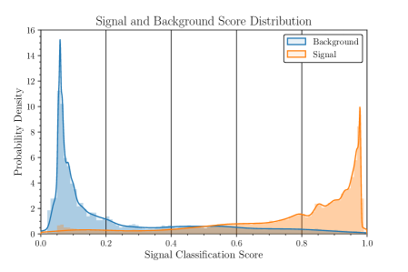
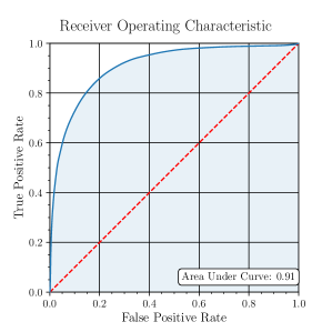
Figure 21: Left: Example distribution of BDT classification scores for the discrimination of mono- and di-jet samples, respectively “Background” and “Signal”, at $p_{\textrm{T}}=1600$ GeV. Training features include the $\delta_{AB}^{N}$ for ($N=1\text{--}5$). Right: Associated Receiver Operating Characteristic curve for true-positives versus false positives.

X Computability and Safety

This section addresses theoretical considerations associated with computability of the SIFT observable $\delta_{AB}$. Expressions are developed for various limits of interest. Infrared and collinear safety is confirmed and deviations from recursive safety are calculated and assessed. It is suggested that SIFT’s embedded filtering criterion may help to regulate anomalous behaviors in the latter context, improving on the Geneva algorithm.

Soft and collinear singularities drive the QCD matrix element governing the process of hadronic showering. In order to compare experimental results against theoretical predictions it is typically necessary to perform all-order resummation over perturbative splittings. In the context of computing observables related to jet clustering, the calculation must first be organized according to an unambiguous parametric understanding of the priority with which objects are to be merged, i.e., a statement of how the applicable distance measure ranks pairings of objects that are subject to the relevant poles. Specifically, cases of interest include objects that are $i$) mutually hard but collinear, $ii$) hierarchically dissimilar in scale, and $iii$) mutually soft but at wide angular separation. Pairs in the first two categories are likely to be physically related by QCD, but those in the third are not.

In order to facilitate considerations of this type, we outline here how the Eq. (15) measure behaves in relevant limits. The angular factor $\Delta\widetilde{R}_{AB}^{2}$ carries intuition for small differences by construction (cf. Eq. 11), and its dependence on aggregated mass has been further clarified in and around Eq. (12). We turn attention then to the energy-dependent factor $\epsilon^{AB}$, as expressed in Eq. (13), in two limits of interest. First, we take the case of hierarchically dissimilar transverse energies, expanding in the ratio ($\alpha\equiv E_{\textrm{T}}^{A}/E_{\textrm{T}}^{B}$) about $0$.

$$2\times\epsilon^{AB}\Rightarrow 2\,\alpha+\cdots$$ (24)

Next, we expand for small deviations ($\zeta\equiv E_{\textrm{T}}^{A}/E_{\textrm{T}}^{B}-1$) from matched transverse energies.

$$2\times\epsilon^{AB}\Rightarrow 1-\frac{\zeta^{2}}{2}+\cdots$$ (25)

The SIFT algorithm is observed be be safe in the soft/infrared and collinear (IRC) radiation limits, because the object separation measure explicitly vanishes as ($\alpha\Rightarrow 0$) or ($\Delta R\Rightarrow 0$), up to terms proportional to the daughter mass-squares (cf. Eq. 12) in the latter case. This feature ensures that splittings at small angular separation or with hierarchically distinct transverse energies will be reunited during clustering at high priority.

With a clustering sequence strictly ranked by generated mass, JADE was plagued by an ordering ambiguity between the first and third categories described above, which presented problems for resummation. Geneva resolved the problem of mergers between uncorrelated mutually soft objects at wide separation in the same way that SIFT does, by diverging when neither entry in the denominator carries a large energy.

Figure 22: Hard object $\lambda$ emits a soft and collinear object $\kappa$ at separation $\Delta\eta$, which experiences a secondary collinear splitting into a pair of objects with comparable hardness ($z\simeq\nicefrac{{1}}{{2}}$).

Yet, both SIFT and Geneva fall short of meeting the recursive IRC safety conditions described in Ref. [29] at the measure level. The challenge arises when a soft and collinear emission splits secondarily into a very collinear pair, as first observed in Ref. [30]. This scenario is visualized in FIG. 22, with hard object $\lambda$ recoiling off a much softer emission $\kappa$ (having $E_{\textrm{T}}^{\kappa}/E_{\textrm{T}}^{\lambda}\ll 1$) at a narrow pseudo-rapidity separation ($\Delta\eta\ll 1$). Azimuthal offsets are neglected here for simplicity. The secondary radiation products are of comparable hardness for the situation of interest, carrying momentum fractions ($z\simeq\nicefrac{{1}}{{2}}$) and ($1-z$) relative to their parent object $\kappa$.

It can be that the members of this secondary pair each successively combine with the hard primary object rather than first merging with each other. This ordering ambiguity implies that the value of the measure $\delta_{AB}$ after the final recombination of all three objects is likewise sensitive to the details of the secondary splitting. However, the mismatch is guaranteed to be no more than a factor of 2. Accordingly, this is a much milder violation than one associated with a divergence (as for JADE). While it does present difficulties for standard approaches to automated computation, it does not exclude computation.

We conclude this section by sketching the relevant calculation, translating results from Appendix F of Ref. [29] into the language of the current work. The secondary splitting is characterized by a parameter $\mu^{2}_{\kappa}\equiv\left(m_{\kappa}/p_{\textrm{T}}^{\hskip 0.75pt\kappa}\right)^{2}$. We further apply the limit ($\,\mu^{2}_{\kappa}\!\ll\!1\,$), which implies ($E_{\textrm{T}}^{\hskip 0.75pt\kappa}\simeq p_{\textrm{T}}^{\hskip 0.75pt\kappa}$), and treat the radiation products of object $\kappa$ as individually massless. The value of the measure for merging these objects is readily computed with Eq. (4), yielding ($\delta^{z}_{1-z}\simeq 2\,\mu^{2}_{\kappa}$). Note that the coefficient comes from the sum of squares in the measure denominator, in the limit of a balanced splitting. The merger of objects $\lambda$ and $\kappa$ (given prior recombination of the $\kappa$ products) is best treated with Eq. (15), defining $\mu^{2}_{\lambda}\equiv\left(m_{\lambda}/p_{\textrm{T}}^{\hskip 0.75pt\lambda}\right)^{2}$, and applying the limits in Eqs. (12, 24), as follows:

$$\delta_{\lambda}^{\kappa}\simeq\bigg{(}\frac{E_{\textrm{T}}^{\kappa}}{E_{\textrm{T}}^{\lambda}}\bigg{)}\times\bigg{[}\,(\Delta\eta^{\kappa}_{\lambda})^{2}+\mu^{2}_{\kappa}+\mu^{2}_{\lambda}\,\bigg{]}$$ (26)

However, if the remnants of object $\kappa$ instead combine in turn with object $\lambda$, then the final value of the measure (taking $z\geq\nicefrac{{1}}{{2}}$ without loss of generality) is instead ($\,\delta^{z}_{\lambda}\simeq z\times\delta_{\lambda}^{\kappa}\,$). In addition to that overall rescaling, the $\mu^{2}_{\kappa}$ term from Eq. (26) is absent from the analogous summation in this context. If the $\kappa$ splitting is hierarchically imbalanced (with $z\simeq 1$), then the secondary splittings are less resistant to merging first and the terminal measure value becomes insensitive to the merging order.

For balanced splittings, the physical showering history will be “correctly” rewound if ($\,\delta^{z}_{1-z}<\,\delta^{1-z}_{\lambda}\,$). But, there are no applicable kinematic restrictions enforcing that condition, and SIFT’s preference for associating objects at dissimilar momentum scales actually constitutes a bias in the other direction. On the other hand, the filtering criterion can help curb potential ambiguities in this regime. Specifically, the energy scale factor ($\,2\times\epsilon^{z}_{1-z}\simeq 1\,$) associated with products of object $\kappa$ will be subject here to the Eq. (25) limit. So, the “wrong” order of association is strongly correlated with cases where ($\,\epsilon^{1-z}_{\lambda}\ll 1\,$), since this is generally required in order to overcome the tendency for strict collinearity ($\Delta\widetilde{R}^{z}_{1-z}\ll\Delta\widetilde{R}^{1-z}_{\lambda}$) in secondary splittings to commensurate momentum scales. In turn, this enhances the likelihood that the Drop condition from Eq. (22) will veto any such merger. A full clarification of the SIFT filtering criterion’s implications for recursive IRC safety is beyond our current scope, but is of interest for future work.

XI Conclusions and Summary

We have introduced a new scale-invariant jet clustering algorithm named SIFT (Scale-Invariant Filtered Tree) that maintains the resolution of substructure for collimated decay products at large boosts. This construction unifies the isolation of variable-large-radius jets, recursive grooming of soft wide-angle radiation, and finding of subjet-axis candidates into a single procedure. The associated measure asymptotically recovers angular and kinematic behaviors of algorithms in the $k_{\textrm{T}}$-family, by preferring early association of soft radiation with a resilient hard axis, while avoiding the specification of a fixed cone size. Integrated filtering and variable-radius isolation criteria resolve the halting problem common to radius-free algorithms and block assimilation of soft wide-angle radiation. Mutually hard structures are preserved to the end of clustering, automatically generating a tree of subjet axis candidates at all multiplicities $N$ for each isolated final-state object. Excellent object identification and kinematic reconstruction are maintained without parameter tuning across more than a magnitude order of transverse momentum scales, and superior resolution is exhibited for highly-boosted partonic systems. The measure history captures information that is useful for tagging massive resonances, and we have demonstrated with the aid of supervised machine learning that this observable has substantially more power for discriminating narrow 1-, 2-, and 3-prong event shapes than the benchmark technique using $N$-subjettiness. These properties suggest that SIFT may prove to be a useful tool for the continuing study of jet substructure.

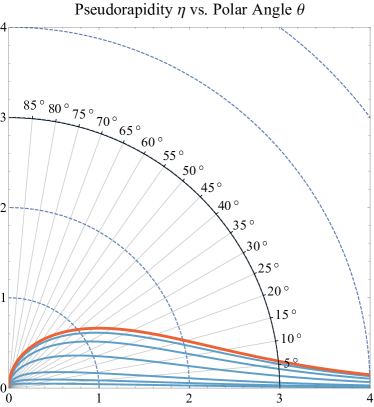
Figure 23: The pseudorapidity $\eta$ (bold, orange) is plotted as a function of the polar angle $\theta$. For comparison, the longitudinal rapidity $y$ (fine, blue) is also shown for various values of ($m/p_{\textrm{T}}$), equal to ($\nicefrac{{1}}{{2}},1,2,5,10,20$) from top to bottom.

Appendix A Review of Collider Coordinates

This appendix provides a brief pedagogical review of hadron collider coordinates. In this application, it is traditional to use a mapping from four-vector coordinates $P_{\mu}\equiv\{E,\vec{p}\}$ into coordinates $\{\eta,\phi,p_{\textrm{T}},m\}$ that are well-behaved under Lorentz boosts along the longitudinal axis $\hat{z}$ of the beam. The pseudo-rapidity $\eta$ (defined following) is a pure function of the zenith angle $\theta$.

$$\eta\equiv\frac{1}{2}\ln\left(\frac{|\,\vec{p}\,|+p_{z}}{|\,\vec{p}\,|-p_{z}}\right)\equiv-\ln\tan\left(\frac{\theta}{2}\right)$$ (27)

Forward (or backward) scattering correspond to $\eta$ equals plus (or minus) infinity, while $\eta=0$ represents entirely transverse scattering. The azimuthal angle $\phi$ measures orientation about the $\hat{z}$ axis. The transverse momentum $p_{\textrm{T}}$ is the magnitude of the 3-vector momentum $\vec{p}$ projection perpendicular to the beam.

$$p_{\textrm{T}}\equiv\sqrt{p_{x}^{2}+p_{y}^{2}}$$ (28)

The final parcel of kinematic information is the Lorentz-invariant mass $m$, which is especially important for jets representing the composition of several lower level physical objects. The 4-vector sum of individually massless objects may accumulate cancellation in the three-momentum that manifests as a non-negligible mass-square in the invariant product.

$$p_{\mu}p^{\mu}\equiv E^{2}-\vec{p}\cdot\vec{p}=m^{2}$$ (29)

The quantity $\Delta R$ provides a radian-like measure of the relativistic “angular separation” between an object pair.

$$\Delta R\equiv\sqrt{{(\Delta\eta)}^{2}+{(\Delta\phi)}^{2}}$$ (30)

The motivation for the definition in Eq. (27) is that differences $\Delta\eta$ in pseudorapidity are “nearly” invariant under longitudinal boosts. To be precise, differences in the rapidity $y$ (defined following) are a strict longitudinal invariant (as are the transverse coordinates $p_{\textrm{T}}$ and $\phi$), and $y$ converges with $\eta$ in the relativistic $(m\ll p_{\textrm{T}})$ limit.

$$y \equiv\frac{1}{2}\ln\Bigg{(}\frac{E+p_{z}}{E-p_{z}}\Bigg{)}$$ (31)

$$=\ln\Bigg{(}\frac{\sqrt{\cosh^{2}\eta+\frac{m^{2}}{p_{\textrm{T}}^{2}}}+\sinh\eta}{\sqrt{1+\frac{m^{2}}{p_{\textrm{T}}^{2}}}}\Bigg{)}$$

FIG. 23 provides a visualization of angular dependence of the pseudorapidity, along with deviation from the rapidity for various amounts of transverse boost. See Ref. [31] for an argument on the primacy of rapidity $y$.

Appendix B Software Implementations

This appendix describes two publicly available implementations of the SIFT algorithm. It also summarizes provided materials that facilitate reproduction of the key analyses in this manuscript. Finally, it outlines challenges to and plans for future integration with the FastJet contributions library.

The AEACuS, RHADAManTHUS, and MInOS packages respectively automate the processes of event analysis, visualization, and machine learning in a collider physics context. These tools are distributed and maintained at GitHub [19] by JWW, and inquiries are welcome. A quick-start tutorial (with a link to a video presentation) is additionally available at Ref. [32]. In brief, each of these programs is invoked from the command line, and is interpreted with Perl 5.8+. Certain back-end features are implemented in Python 3, importing modules that include MatPlotLib and XGBoost, as noted previously. All instructions regarding the computation of observables, application of event selection, generation of plots, and application of machine learning are specified in an associated card file, using a compact meta-language. Control cards used in the preparation of this work are provided with its source package on the arXiv.

These programs are designed for easy integration with the standard MadGraph/MadEvent, Pythia8, and Delphes chain, and cards are similarly included that document our approach to event production, generator-level selections, and the simulation of showering, hadronization, and detector effects. AEACuS auto-generates an extended-LHCO event record that bundles parton, hadron, and detector-level information (with weights) from the primary simulation chain for subsequent analysis. It further facilitates a variety of jet clustering and substructure applications, including an implementation of the SIFT algorithm. This usage is documented further in the example “cut” cards. The output is a space-delimited plain-text record of observables for each passing event, which serves in turn as an input to subsequent plotting and machine-learning operations.

The second existing public implementation of the SIFT algorithm is in the Mathematica notebook used here to produce jet clustering films and still frames. That notebook is likewise distributed on GitHub, bundled with the tools described prior. To run the notebook, simply place a suitable extended-LHCO event record into its working directory and “Evaluate Initialization Cells”. User-adjustable parameters are documented in the notebook, for stipulating the clustering algorithm (members of the $k_{\textrm{T}}$ family are also supported), a cone size (as applicable), any halting and filtering criteria, and whether ultra-soft ghost radiation should be included. An .mp4 film is typically output within a few minutes on a laptop computer, although running the notebook with ghost radiation enabled can be considerably more time consuming.

Additionally, a third implementation is planned that interfaces with FastJet, facilitating broader exploration of the SIFT algorithm within existing workflows. The FastJet implementation of Cacciari and Salam is famous for reducing the naïve $\mathcal{O}(N^{3})$ runtime required for iterative pairwise jet clustering to $\mathcal{O}(N^{2})$, or even to $\mathcal{O}(N\log N)$ in certain cases. It assumes a pairwise clustering measure $\delta_{ij}\equiv\min[f(p_{\textrm{T}}^{i}),f(p_{\textrm{T}}^{j})]\times g(\Delta R_{ij})$ composed as the product of a kinematic function referencing the minimal value of $f(p_{\textrm{T}}^{i,j})$ over the pair times a “geometric” measure $g(\Delta R_{ij})$ that is typically a power of the pairwise angular separation. In contrast to the $k_{\textrm{T}}$-family of measures, where factorization under the “FastJet Lemma” reduces neighbor-finding to the $\Delta R$ plane, the search for SIFT neighbors is necessarily active in (at least) three dimensions. Moreover, the associated measure (cf. Eq. 15) prioritizes furthest neighbors along one of these axes ($u$). Adaptations capable of confronting these unique challenges while maintaining “linearithmic” $\mathcal{O}(N\log N)$ scaling will be presented in a future work.

References

- Cacciari et al. [2008a] M. Cacciari, G. P. Salam, and G. Soyez, “The Anti-k(t) jet clustering algorithm,” JHEP 04, 063 (2008a), eprint 0802.1189
- Thaler and Van Tilburg [2011] J. Thaler and K. Van Tilburg, “Identifying Boosted Objects with N-subjettiness,” JHEP 03, 015 (2011), eprint 1011.2268
- Larkoski et al. [2014] A. J. Larkoski, S. Marzani, G. Soyez, and J. Thaler, “Soft Drop,” JHEP 05, 146 (2014), eprint 1402.2657
- Stewart et al. [2015] I. W. Stewart, F. J. Tackmann, J. Thaler, C. K. Vermilion, and T. F. Wilkason, “XCone: N-jettiness as an Exclusive Cone Jet Algorithm,” JHEP 11, 072 (2015), eprint 1508.01516
- Thaler and Wilkason [2015] J. Thaler and T. F. Wilkason, “Resolving Boosted Jets with XCone,” JHEP 12, 051 (2015), eprint 1508.01518
- Stewart et al. [2010] I. W. Stewart, F. J. Tackmann, and W. J. Waalewijn, “N-Jettiness: An Inclusive Event Shape to Veto Jets,” Phys. Rev. Lett. 105, 092002 (2010), eprint 1004.2489
- Bethke et al. [1992] S. Bethke, Z. Kunszt, D. Soper, and W. Stirling, “New jet cluster algorithms: next-to-leading order QCD and hadronization corrections,” Nuclear Physics B 370, 310 (1992), ISSN 0550-3213, URL https://www.sciencedirect.com/science/article/pii/055032139290289N
- Cacciari et al. [2012] M. Cacciari, G. P. Salam, and G. Soyez, “FastJet User Manual,” Eur. Phys. J. C 72, 1896 (2012), eprint 1111.6097
- Cacciari and Salam [2006] M. Cacciari and G. P. Salam, “Dispelling the myth for the jet-finder,” Phys. Lett. B 641, 57 (2006), eprint hep-ph/0512210
- Catani et al. [1993] S. Catani, Y. L. Dokshitzer, M. H. Seymour, and B. R. Webber, “Longitudinally invariant clustering algorithms for hadron hadron collisions,” Nucl. Phys. B406, 187 (1993)
- Ellis and Soper [1993] S. D. Ellis and D. E. Soper, “Successive combination jet algorithm for hadron collisions,” Phys. Rev. D 48, 3160 (1993), eprint hep-ph/9305266
- Dokshitzer et al. [1997] Y. L. Dokshitzer, G. D. Leder, S. Moretti, and B. R. Webber, “Better jet clustering algorithms,” JHEP 08, 001 (1997), eprint hep-ph/9707323
- Wobisch and Wengler [1998] M. Wobisch and T. Wengler, in Workshop on Monte Carlo Generators for HERA Physics (Plenary Starting Meeting) (1998), pp. 270–279, eprint hep-ph/9907280
- Bethke et al. [1988] S. Bethke et al. (JADE), “Experimental Investigation of the Energy Dependence of the Strong Coupling Strength,” Phys. Lett. B213, 235 (1988)
- Bartel et al. [1986] W. Bartel et al. (JADE), “Experimental Studies on Multi-Jet Production in e+ e- Annihilation at PETRA Energies,” Z. Phys. C 33, 23 (1986)
- Dreyer et al. [2018] F. A. Dreyer, L. Necib, G. Soyez, and J. Thaler, “Recursive Soft Drop,” JHEP 06, 093 (2018), eprint 1804.03657
- Butterworth et al. [2008] J. M. Butterworth, A. R. Davison, M. Rubin, and G. P. Salam, “Jet substructure as a new Higgs search channel at the LHC,” Phys. Rev. Lett. 100, 242001 (2008), eprint 0802.2470
- Walker [2022a] J. W. Walker, “Large Hadron Collider Jet Clustering Visualizations,” (2022a), URL https://youtube.com/playlist?list=PLwgaPsMt19Rsu53Wh7r_rj8oF-rX_tDOt
- Walker [2023] J. W. Walker, “AEACuS, RHADAManTHUS, and MInOS: Automated Tools for Collider Event Analysis, Plotting, and Machine Learning,” (2023), URL https://github.com/joelwwalker/AEACuS
- Alwall et al. [2014] J. Alwall, R. Frederix, S. Frixione, V. Hirschi, F. Maltoni, O. Mattelaer, H. S. Shao, T. Stelzer, P. Torrielli, and M. Zaro, “The automated computation of tree-level and next-to-leading order differential cross sections, and their matching to parton shower simulations,” JHEP 07, 079 (2014), eprint 1405.0301
- Sjöstrand et al. [2015] T. Sjöstrand, S. Ask, J. R. Christiansen, R. Corke, N. Desai, P. Ilten, S. Mrenna, S. Prestel, C. O. Rasmussen, and P. Z. Skands, “An Introduction to PYTHIA 8.2,” Comput. Phys. Commun. 191, 159 (2015), eprint 1410.3012
- de Favereau et al. [2014] J. de Favereau, C. Delaere, P. Demin, A. Giammanco, V. Lemaître, A. Mertens, and M. Selvaggi (DELPHES 3), “DELPHES 3, A modular framework for fast simulation of a generic collider experiment,” JHEP 02, 057 (2014), eprint 1307.6346
- Cacciari et al. [2008b] M. Cacciari, G. P. Salam, and G. Soyez, “The Catchment Area of Jets,” JHEP 04, 005 (2008b), eprint 0802.1188
- Bertolini et al. [2014] D. Bertolini, P. Harris, M. Low, and N. Tran, “Pileup Per Particle Identification,” JHEP 10, 059 (2014), eprint 1407.6013
- Krohn et al. [2010] D. Krohn, J. Thaler, and L.-T. Wang, “Jet Trimming,” JHEP 02, 084 (2010), eprint 0912.1342
- Ellis et al. [2010] S. D. Ellis, C. K. Vermilion, and J. R. Walsh, “Recombination Algorithms and Jet Substructure: Pruning as a Tool for Heavy Particle Searches,” Phys. Rev. D81, 094023 (2010), eprint 0912.0033
- Hunter [2007] J. D. Hunter, “Matplotlib: A 2D graphics environment,” Computing in Science & Engineering 9, 90 (2007)
- Chen and Guestrin [2016] T. Chen and C. Guestrin, in Proceedings of the 22nd ACM SIGKDD International Conference on Knowledge Discovery and Data Mining (ACM, New York, NY, USA, 2016), KDD ’16, pp. 785–794, ISBN 978-1-4503-4232-2, URL http://doi.acm.org/10.1145/2939672.2939785
- Banfi et al. [2005] A. Banfi, G. P. Salam, and G. Zanderighi, “Principles of general final-state resummation and automated implementation,” JHEP 03, 073 (2005), eprint hep-ph/0407286
- Catani et al. [1992] S. Catani, B. R. Webber, Y. L. Dokshitzer, and F. Fiorani, “Average multiplicities in two and three jet e+ e- annihilation events,” Nucl. Phys. B 383, 419 (1992)
- Gallicchio and Chien [2018] J. Gallicchio and Y.-T. Chien, “Quit Using Pseudorapidity, Transverse Energy, and Massless Constituents,” (2018), eprint 1802.05356
- Walker [2022b] J. W. Walker, “Automated Collider Event Selection, Plotting, & Machine Learning with AEACuS, RHADAManTHUS, & MInOS,” Proceedings of Science, Comp Tools 2021 027, 071 (2022b)