Rubin LSST observing strategies to maximize volume and uniformity coverage of Star Forming Regions in the Galactic Plane

Abstract

A complete map of the youngest stellar populations of the Milky Way in the era of all-sky surveys, is one of the most challenging goals in modern astrophysics. The characterization of the youngest stellar component is crucial not only for a global overview of the Milky Way structure, of the Galactic thin disk, and its spiral arms, but also for local studies. In fact, the identification of the star forming regions (SFRs) and the comparison with the environment in which they form are also fundamental to put them in the context of the surrounding giant molecular clouds and to understand still unknown physical mechanisms related to the star and planet formation processes. In 10 yrs of observations, Vera C. Rubin Legacy Survey of Space and Time (Rubin-LSST) will achieve an exquisite photometric depth that will allow us to significantly extend the volume within which we will be able to discover new SFRs and to enlarge the domain of a detailed knowledge of our own Galaxy. We describe here a metrics that estimates the total number of young stars with ages $t<10$ Myr and masses $>$0.3 M_⊙ that will be detected with the Rubin LSST observations in the gri bands at a 5 $\sigma$ magnitude significance. We examine the results of our metrics adopting the most recent simulated Rubin-LSST survey strategies in order to evaluate the impact that different observing strategies might have on our science case.

1 Introduction

In the era of all-sky astrophysical surveys, mapping the youngest stellar populations of the Milky Way in the optical bands is one of the main core science goals. Up to now, a full overall understanding of the Galactic components has been hampered by observational limits and, paradoxically, we have a better view of the morphological structure of external galaxies than of the Milky Way. In particular, it is crucial to trace the poorly known Galactic thin disk, and its spiral arms, where most of the youngest stellar populations are expected to be found.

The youngest galactic stellar component is mainly found in star forming regions (SFRs), namely stellar clusters and over-dense structures originating from the collapse of the molecular clouds, the coldest and densest part of the interstellar medium (Mac Low & Klessen, 2004). It is by now relatively easy to identify in the near-, mid-, far-infrared (IR), and radio wavelengths the young stellar objects (YSOs) within SFRs, during the first phases of the star formation process. In fact, at these wavelengths, due to the presence of the optically thick infalling envelope or circumstellar disk around the central star, they show, at these wavelengths, an excess with respect to the typical photospheric emission. During the subsequent phases, they start to emit also in the optical bands, while the circumstellar disk is still optically thick (Bouvier et al., 2007). YSOs are no longer easily identifiable in the IR or at radio wavelengths, when the final dispersal of the disk material occurs and non-accreting transition disks form (Ercolano et al., 2021). At these latter stages, a complete census of the YSOs can be achieved only using deep optical observations. Such census is therefore crucial for a thorough comprehension of the large scale three-dimensional structure of the young Galactic stellar component.

The identification of SFRs and the comparison with the environment in which they form are also fundamental to put them in the context of the surrounding giant molecular clouds and to answer still controversial open questions about the star formation (SF) process, such as, i) did the SFRs we observe originate from monolithic single SF bursts or from multiple spatial and temporal scales, i.e. in a hierarchical mode (e.g. Kampakoglou et al., 2008)? ii) When can the feedback from massive stars affect the proto-planetary disk evolution (Tanaka et al., 2018) or trigger subsequent SF events, as thought, for example, for the Supernova explosion in the $\lambda$ Ori region (Kounkel et al., 2020)? iii) Is the overall spatial distribution of SFRs correlated to an overall large scale structure, such as the Gould Belt or the damped wave, very recently suggested by Alves et al. (2020)?

The Vera C. Rubin Observatory (Ivezić et al., 2019) will conduct a Legacy Survey of Space and Time (LSST) with a very impressive combination of flux sensitivity, area, and temporal sampling rate (Bianco et al., 2022).

A flexible scheduling system is designed to maximize the scientific return under a set of observing constraints. Vera C. Rubin will perform in the 10 years a set of surveys. These include the Wide-Fast-Deep (WFD) that is the “main” LSST survey, primarily focused on low-extinction regions of the sky for extra-galactic science, the Deep Drilling Fields (DDFs), that are a set of few individual fields that will receive high cadence and additional “minisurveys”, that cover specific sky regions such as the ecliptic plane, Galactic plane (GP), and the Large and Small Magellanic Clouds with specific observing parameters (Bianco et al., 2022).

The implementation of the Rubin LSST observing strategy must meet the basic LSST Science Requirements but a significant flexibility in the detailed cadence of observations is left to ensure the best optimisation of the survey. The scientific community has been involved to give feedback on specific science cases on the distribution of visits within a year, the distribution of images between filters, and the definition of a “visit” as single or multiple exposures. To this aim, simulated realisations of the 10-yr sequence of observations acquired by LSST, for different sets of basis functions that define the different survey strategies, indicated as OpSim, are made available to the community. Such simulated observations can be analysed through an open-access software package, the metrics analysis framework (MAF, Jones et al., 2014), where specific metrics can be calculated to quantify the suitability of a given strategy for reaching a particular science objective.

In the original baseline, i.e. the reference benchmark survey strategy, the mini survey of the GP was covered by a number of visits a factor $\sim$5 smaller than those planned for WFD. The main reason of this choice is to avoid highly extincted regions with E(B-V)$>$0.2 since this amount of dust extinction is problematic for extragalactic science, as motivated in Jones et al. (2021). Nevertheless, mapping the Milky Way is one of the four broad science pillars that LSST will address (Bianco et al., 2022).

We aim to show here that alternative implementations in which the number of visits planned for the WFD is extended also to the Galactic thin disk ($|b|\lesssim$ 5-10^∘), will increase significantly the impact of Rubin LSST on the understanding of the Galactic large-scale structures and in particular of the large molecular clouds in which stars form. The stellar components of the SFRs, and, in particular, the most populated low mass components down to the M-dwarf regime with age t$\lesssim$10 Myrs, that will be discovered with Rubin LSST observations, are one of the most relevant output of the star formation process and assessing their properties (spatial distribution in the Galaxy, masses, ages and age spread) is crucial to trace the global structure of the youngest populations as well as to pinpoint several under-debate disputes such as the universality of the Initial Mass Function (IMF), the duration of the evolutionary phases involved in the star formation process and the dynamical evolution (Chabrier, 2003; Tassis & Mouschovias, 2004; Ballesteros-Paredes et al., 2007; Parker et al., 2014).

Even though the thin disk of the Galaxy is strongly affected by high dust extinction and crowding issues, it is the only Galactic component where most of such structures are found and where young stars are exclusively found.

A big step forward has been made in the comprehension of the Galactic components thanks to the Gaia data that allowed us to achieve a clearer and homogeneous overview of the Galactic structures, including the youngest ones, but at distances from the Sun limited to 2-3 kpc (Zari et al., 2018; Kounkel & Covey, 2019; Kounkel et al., 2020; Kerr et al., 2021; Prisinzano et al., 2022). The exquisite science return from the very deep Rubin LSST static photometry, derived from co-added images, is the only opportunity to push such large-scale studies of young stars to otherwise unreachable and unexplored regions.

With respect to the old open clusters, the study of the SFRs is favored by the intrinsic astrophysical properties of the low mass YSOs, representing the bulk of these populations. In fact, during the pre-main sequence (PMS) phase, M-type young stars are more luminous in bolometric light than the stars of the same mass in the main sequence (MS) phase. For example, for a given extinction, a 1 Myr (10 Myrs) old 0.3 M_⊙ star is 3.4 mag (1.6 mag) brighter than a 100 Myr star of the same mass (Tognelli et al., 2018; Prisinzano et al., 2018b). Therefore, if on one hand the extinction limits our capability to detect such low mass stars, on the other hand, the higher intrinsic luminosity of young stars (t$<$10 Myr) compensates for this effect, allowing a significant increase in the volume of PMS stars detectable with respect to old MS stars. Such property has been exploited in Damiani (2018); Prisinzano et al. (2018a); Venuti et al. (2019) where a purely photometric approach using gri magnitudes combined with the most deep near-IR magnitudes available in the literature, has been adopted to statistically identify YSOs at distances where M-type MS stars are no longer detectable, because they are intrinsically less luminous than the analogous M-type PMS stars.

We note, however, that also studies of other relevant structures, such as for example, stellar clusters, as tracers of the Galactic chemical evolution (Prisinzano et al., 2018a), as well as transient phenomena (see Street et al. 2021 Cadence Note) would benefit from the observed strategy discussed in this paper.

The goal of this paper is to evaluate the impact on the YSO science of different Rubin LSST observing strategies and, in particular, of the different WFD-like cadences extended to the GP, as an improvement with respect to the baseline observing strategy.

2 metrics definition

The metrics we present in this work is defined as the number of detectable YSOs with masses down to 0.3 M_⊙ and ages t$\leq$10 Myr, distributed in the GP and, in particular, in the thin disk of the Milky Way.

The number of YSOs estimated in this work is not based on empirical results but on the theoretical description of the star number density $\rho$ (number of stars per unit volume) in the Galactic thin disk, integrated within the volume accessible with Rubin LSST observations. In particular, the total number of young stars observable within a given solid angle $\Omega$ around a direction (e.g. a Healpix) defined by the Galactic coordinates $(l,b)$ will be obtained by integrating such density along cones, using volume elements

$$dV=\Omega r^{2}dr$$ (1)

where $r$ is the distance from the Sun. Therefore we define this number of stars as

$$N(<r_{max})=\int_{0}^{r_{max}}\rho(r,l,b)\;\;dV$$ (2)

where $r_{max}$ is the maximum distance from the Sun that is defined from the observation depth.

2.1 Density law of YSOs in the Galactic Thin Disk

In the Galactic thin disk, the star density distribution or number density, usually called the density profile or density law, can be described by a double exponential (e.g. Cabrera-Lavers et al., 2005), as follows:

$$\rho(r,l,b)=A\times exp\left(-\frac{r|sinb|}{h}-\frac{R}{r_{1}}\right)$$ (3)

where $A$ is the total density normalization (to be computed below), $h$ is the thin disk scale height that we assume equal to 300 pc (Bland-Hawthorn & Gerhard, 2016), $R$ is the Galactocentric distance, and $r_{1}$ is the thin-disk radial scale length that we assume equal to 2.6 kpc (Freudenreich, 1998). The Galactocentric distance $R$ can be expressed in terms of $r$, $l$, and Galactic Center distance from the Sun $D$, as:

$$R=\sqrt{(D-r\cos l)^{2}+(r\sin l)^{2}}.$$ (4)

To derive the density normalization constant $A$, we integrate the thin-disk density $\rho$ over the whole Galaxy, to obtain the total number of stars as:

$$N=4\pi Ahr_{1}^{2}$$ (5)

Recent results by Giammaria et al. (2021, see their Table 2) show that, within a factor of two, we can assume in the Galaxy a constant star formation rate. Therefore, in the whole Galaxy the total number of stars with ages t$<$10 Myr, N_yng, can be estimated as

$${\rm N}_{\rm yng}=\frac{t_{\rm yng}}{t_{\rm MW}}\times{\rm N}_{\rm tot}$$ (6)

where $t_{\rm yng}$=10 Myr is the upper age limit for the youngest stellar component considered here, $t_{\rm MW}$ is the Galaxy age that we assume to be $\sim$10 Gyr and N_tot is the total number of the stars in the Galaxy roughly equal to 10¹¹. With these assumptions N_yng amounts to 10⁸ stars. Moreover, to take into account that we are going to miss about 20% of the IMF below 0.3 $M_{\odot}$ (Weidner et al., 2010), we should add a corrective factor of 0.8 for the number of actually observable stars.

Therefore, we may reasonably approximate in the Equ. 5 for the total thin-disk content $N\sim 0.8\times N_{yng}$, from which $A\sim\frac{0.8\times 10^{8}}{4\pi hr_{1}^{2}}$, to be used in Eq. 3.

2.2 Rubin LSST accessible volume

The element of volume within a given solid angle $\Omega$, as well as the density law $\rho$, defined by the equations 1 and 3, respectively, depend on the distance from the Sun. At a given mass and age and for a given extinction, the maximum distance that can be achieved with Rubin LSST data is a function of the photometric observational depth and thus of the adopted observing strategy. To evaluate such distance, and thus to define such volume, our metrics has been defined with the following criteria:

• use of the Rubin LSST gri filters, assuming to use the $r-i$ vs. $g-r$ diagram to photometrically select the YSOs, as in Damiani (2018); Prisinzano et al. (2018a); Venuti et al. (2019). This is a restrictive assumption, since more than 3 Rubin LSST filters will be used for the selection;

• use of a dust map to take into account the non-uniform extinction pattern that characterizes the GP, in particular towards the Galactic Center;

• estimate the maximum distance that will be achieved assuming different OpSims.

The definition of the metrics is therefore based on the following rationale: specify the desired accuracy magnitude/$\sigma$ = 5 for gri filters and compute the corresponding limiting magnitudes from coadded images; correct for extinction the apparent magnitudes using a dust map; compute the maximum distance at which a 10 Myr old star of 0.3 M_⊙ can be detected, assuming the absolute magnitudes in the gri filters, M_g=10.32, M_r=9.28 and M_i=7.97, predicted for such a star by a 10 Myr solar metallicity isochrone (Tognelli et al., 2018); calculate the corresponding volume element within a Nside=64 Healpix; integrate the young star density within the volume element, through equation 2.

2.2.1 Dust map

The dust extinction is an increasing function of the distance and then nearby stars are affected by E(B-V) values smaller than those of more distant stars. The Schlegel et al. (1998) map has a massive use in Astronomy, but provide an integrated extinction along a line of sight at the maximum distance corresponding to the adopted 100 $\mu$m observations. As a consequence, they are more useful for extragalactic studies (Amôres et al., 2021). Assuming a 2D dust extinction i.e. a map that depends only on the positions (e.g. the galactic coordinates $l,b$) leads to a significant overestimation of the real extinction at different distances, especially in the directions with A${}_{\rm V}>$0.5 (e.g Arce & Goodman, 1999; Amôres & Lépine, 2005), such as in the GP and, in particularly, in the Galactic spiral arms.

In the last years, many efforts have been done to derive 3D extinction maps that take into account the strong dependence on the distance, as summarised in Amôres et al. (2021).

A 3D dust map, appropriated for the Rubin LSST metrics, has been developed (Mazzi et al. in preparation) by using the Lallement et al. (2019) map, the mwdust.Combined19 map, based on the Drimmel et al. (2003); Green et al. (2019); Marshall et al. (2006) maps, combined with the method described in Bovy et al. (2016), and the Planck Collaboration et al. (2016) map Planck. The 3D map has been integrated in the MAF as DustMap3D to distinguish it from the default Rubin 2D Dust_values based on Schlegel et al. (1998) map. The two maps can be imported into MAF with the following commands:

from rubin_sim.photUtils import Dust_values
from rubin_sim.maf.maps import DustMap3D.

To test the effect on our metrics of using the 2D or the 3D dust map and select the one predicting the more realistic results, we computed our metrics by considering the default 2D dust map implemented within the MAF, as well as the new 3D dust map. Fig. 1 (left panel) shows the results of our metrics on the OpSim simulation named baseline_v2.0_10yrs, obtained by assuming the 2D dust map, while Fig. 1 (right panel) shows the corresponding result, assuming the 3D dust map.

The results point out that by assuming the 3D distant-dependent extinction map, the number of detectable YSOs decreases only smoothly towards the inner GP. On the contrary, the sharp decrease in the detected YSOs in the inner GP is evidence of an unrealistic star distribution due to the adoption of an unsuitable overestimated extinction map (2D dust map). Therefore, the final version of the code defining our metrics includes the 3D dust map.

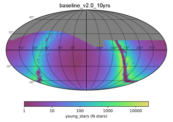
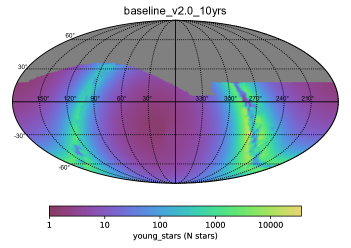
Figure 1: Map of the number of detectable YSOs per HEALPix computed with our metrics, using the 2D dust map (left panel) and the 3D dust map (right panel). In both cases the baseline_v2.0_10yrs has been adopted. The sky is shown in the equal-area Mollweide projection in equatorial coordinates and the HEALPIX grid resolution is $N_{side}=64$.

2.2.2 Crowding effects

Our metrics has been defined by assuming the formal limiting magnitude at 5$\sigma$ photometric precision, but in several wide areas of the Galactic Plane, the limiting magnitude should be set by the photometric errors due to the crowding. To take into account such effect a specific crowding metrics has been developed within MAF based on the TRILEGAL stellar density maps (Dal Tio et al., 2022) to compute the errors that will result from stellar crowding.

Such crowding metrics has been included in our code since we expect that the observations become severely incomplete when the photometric errors due to the crowding exceed 0.25 mag. These photometric errors are derived using the formalism by Olsen et al. (2003) and the 0.25 mag criterion has been empirically checked using deep observations of the Bulge (Clarkson et al., in preparation for this ApJS special issue). Therefore, to detect the faintest stars in very crowded regions we used the minimum (brightest) magnitude between those obtained with maf.Coaddm5Metric() and maf.CrowdingM5Metric(crowding_error=0.25).

The limiting magnitudes achieved after including the crowding effects can be $\sim$2-3 magnitudes brighter than those obtained without considering confusion effects. As a consequence, the number of YSOs detected by including the confusion metrics, shown in Fig. 2, can be significantly smaller than that predicted by the metrics that does not include such effect, shown in Fig 1, right panel.

We note that the two-pronged fork feature in the map shown in Fig. 2 is due to the fact that in the layers immediately above and below the GP, the crowding is the dominant effect and the number of possible detections goes down here from more than 10000 to surprisingly low values of 10-100 (sources/HEALPix). On the contrary, in the central layer of the GP, the extinction is the dominant effect, while the crowding effect is negligible since a smaller number of stars is visible. As a consequence, after applying the crowding metrics, the number of detections in this central layer remains almost constant (around 1000 sources), while the missed detection fraction is significantly larger in the layers immediately higher and lower than the GP. This result is consistent with what recently pointed out by Cantat-Gaudin et al. (2023) for the Gaia data.

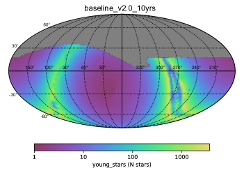
Figure 2: Map of the number of detectable YSOs per HEALPix computed with our metrics, using the baseline_v2.0_10yrs, the 3D dust map and the crowding metrics. The sky is shown in the equal-area Mollweide projection in equatorial coordinates and the HEALPIX grid resolution is $N_{side}=64$.

3 Results

Figure 3: Map of the number of visits per HEALPix planned for the four representative OpSim relevant for our science case. The small yellow patches are the Deep Drilling Fields (DDFs) to which an higher number of observations is assigned. Note as the Rubin-LSST footprint of the baselines (panels a and b) is significantly different with respect to that of the vary_gp_gpfrac1.00_v2.0_10yrs and the plane_priority_priority0.3_pbt_v2.1_10yrs OpSim (panels c and d), where the number of visits at the WFD level is assigned also to the high dust extinction GP area. The sky is shown in the equal-area Mollweide projection in equatorial coordinates and the HEALPIX grid resolution is $N_{side}=64$.

The Python code that computes the metrics described in the previous sections is publicly available in the central rubin_sim MAF metrics repository

with the name YoungStellarObjectsMetric.py.

To evaluate the impact of the different family sets of OpSim on our science case, we considered the current state of LSST v2.0 and v2.1 OpSim databases and metrics results. In particular, we considered the following runs:

• baseline_v2.0_10yrs, the reference benchmark survey strategy in which the WFD survey footprint has been extended to include the central GP and bulge, and is defined by low extinction regions. Such configuration includes also five Deep Drilling Fields and additional mini-survey areas of the North Ecliptic Plane, of the GP, and of the South Celestial Pole.

• baseline_v2.1_10yrs, in which the Virgo cluster and the requirement on the seeing fwhmEff $<$ 0.8^′′  for the images in r and i bands have been added with respect to the baseline_v2.0_10yrs.

• Vary GP family of simulations in which the fraction of the amount of survey time spent on covering the background (non-WFD-level) GP area ranges from 0.01 to 1.0 (labeled as frac0.01 - frac1.00), where 1.0 corresponds to extending the WFD cadence to the entire GP. The baseline characteristics, including the ratio of visits over the remainder of the footprint, are kept the same. In our case, we considered the vary_gp_gpfrac1.00_v2.0_10yrs survey, planning the maximum amount of time on the GP.

• Plane Priority, the family of OpSim that uses the GP priority map, contributed by LSST SMWLV & TVS science collaborations, as the basis for further variations on GP coverage. For this family of simulations, different levels of priority of the GP map are covered at WFD level, unlike the baseline and Vary GP family where only the ”bulge area” is covered at WFD level. In our case, we considered the plane_priority_priority0.3_pbt_v2.1_10yrs survey, since it maximises the results of our metrics.

To evaluate the best observing strategy to be adopted for the YSO science, we defined as Figure of Merit (FoM), the ratio between the number of young stars detected with a given OpSim with respect to the number of young stars detected with the baseline_2.0_10yrs survey, this latter taken as reference. The map of the number of visits planned for these four representative OpSim surveys are shown in Figure 3, while the results of the metrics, i.e. the number of YSOs with ages $t<10$ Myr and masses $>0.3$ M_⊙, obtained with these four representative OpSim surveys are given in Table 1 and shown in Figure 4. The FoM obtained with our metrics using the four OpSim described before are also given in Table 1. Both, the number of YSOs and the FOM predicted by the metrics not including and including the crowding effects are given in order to quantify the differences due to the confusion effects.

OpSim ID	N	FoM	NCrow	FoMCrow
baseline_v2.0_10yrs	8.08$\times 10^{6}$	1.00	4.84$\times 10^{6}$	1.00
baseline_v2.1_10yrs	8.10$\times 10^{6}$	1.00	4.87$\times 10^{6}$	1.01
vary_gp_gpfrac1.00_v2.0_10yrs	8.92$\times 10^{6}$	1.10	5.58$\times 10^{6}$	1.15
plane_priority_priority0.3_pbt_v2.1_10yrs	9.51$\times 10^{6}$	1.18	6.02$\times 10^{6}$	1.24

Table 1: Number of YSOs with ages t$<$10 Myr and masses $>$0.3 M_⊙ that can be detected at distances $<r_{max}$ set by different OpSim surveys, and relative FoM values, estimated by neglecting the crowding metrics (N and FoM columns) and by including it (N_Crow and FoM_Crow columns).

Figure 4: Map of the number of YSOs per HEALPix as computed by our metrics, adopting the OpSim surveys listed in Table 1 and indicated by the names superimposed on top of each panel. The sky is shown in the equal-area Mollweide projection in equatorial coordinates and the HEALPIX grid resolution is $N_{side}=64$. Note that the map in panel (a) is identical to the map shown in Fig. 2.

4 Discussion and conclusions

In this paper we presented a metrics aimed to estimate the number of YSOs we can discover with Rubin LSST static science data. To take into account the effects due to the extinction, we evaluated the metrics by using both, the default LSST MAF 2D dust map and the 3D dust map where a more realistic dependence on the distance is included. The results of this comparison show that the 2D dust map overestimates E(B-V) values for close (few kpc) accessible stars, even in the direction of the GP. For this reason, the final metrics has been implemented by considering the 3D dust map integrated into MAF.

To evaluate the faintest magnitudes that can be attained in crowded regions, a specific crowding metrics has been imported in the code. In order to quantify the crowding effects, we evaluated our metrics also by neglecting the crowding effects. The results show that, if the crowding metrics is included, the number of detected YSOs (N_Crow in Table 1) is a factor 0.6-0.63 smaller than the number of YSOs predicted if the crowding is not considered (column N in Table 1). Since the most realistic predictions are those obtained by including the crowding effects, the final version of the code that defines the YSOs metrics includes the crowding metrics.

The impact of changing from the baseline v2.0 to v2.1 is negligible, while adopting the vary_gp_gpfrac1.00_v2.0_10yrs survey, the only one available covering 100% the GP with WFD exposure times, the predicted number of YSOs (t$<$10 Myr) down to 0.3 M_⊙ is a factor 1.15 larger than that predicted adopting the baseline_v2.0_10yrs, leading to a gain of 0.74$\times 10^{6}$ new discovered YSOs at very large distances. An even higher impact can be obtained by adopting the most recently contributed plane_priority_priority0.3_pbt_v2.1_10yrs predicting different levels of priority of the GP map. With this survey, the predicted number of YSOs is a factor 1.24 higher with respect to the baseline, corresponding to a gain of $\sim 1.17\times 10^{6}$ additional YSOs.

To determine at what distance and beyond which distance from the Sun this gain is most significant, we included in our metrics also the computation of the maximum distance that can be reached for a 10 Myr old star of 0.3 M_⊙ within each Healpix. We derived the distribution of such distances, weighted by the number of YSOs that can be detected in each line of sight. The distributions obtained for the four OpSim considered in this work are shown in Fig. 5.

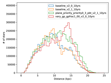
Figure 5: Number of detected YSOs as a function of the distance for the four OpSim indicated in Table 1.

We note that the number of YSOs detected at distances from the Sun larger than $\sim$10 kpc is significantly larger for the OpSim plane_priority_priority0.3_pbt_v2.1_10yrs and vary_gp_gpfrac1.00_v2.0_10yrs than for the two baselines. The curve of the vary_gp_gpfrac1.00_v2.0_10yrs OpSim sits below the baseline curves for d=7-10 kpc. This could be due to the fact that in the two baselines, the number of visits in the regions outside the GP is higher (800-900) with respect to that planned for the vary_gp_gpfrac1.00_v2.0_10yrs (700-800), where the coverage is uniform. This comparison clearly shows that the science enabled by adopting an observing strategy consistent with the plane_priority_priority0.3_pbt_v2.1_10yrs or vary_gp_gpfrac1.00_v2.0_10yrs OpSims would be precluded if we followed the prescriptions of other simulations. These results highlight the greatest impact of Rubin LSST WFD cadence data extended to the GP, mainly arising from the unknown farthest young stars that will be discovered. We note that the two baselines and the vary_gp_gpfrac1.00_v2.0_10yrs OpSims show an asymmetric distribution with a peak that is around 9 kpc and 14 kpc, respectively. The plane_priority_priority0.3_pbt_v2.1_10yrs OpSim shows a more smoothed and symmetric shape, that is likely due to the different levels of priority given to the GP for this survey strategy.

We retain that a gain of 24% in the number of discovered YSOs, mainly arising at distances larger than 10 kpc, represents a strong justification to extend the WFD strategy to the GP, and to ensure the uniformity of the observing strategy in the Galaxy.

Finally, we note that our metrics scales more strongly with the area rather than with the number of visits per pointing and therefore, in case the plane_priority_priority0.3_pbt_v2.1_10yrs survey cannot be adopted, we advocate the adoption of the vary_gp_gpfrac1.00_v2.0_10yrs, to preserve the uniform coverage of the GP.

We stress that our request is to extend the number of visits planned for the WFD to the GP but without constraints on the temporal observing cadence, since our analysis is based on the use of the co-added gri Rubin LSST images. However, different visits per night should be in different filters from the gri set. The same applies in case 2 or 3 visits/night are made, as this would enhance the number but also the accuracy of color measurements available, and hence heightens the fraction of YSOs that can be detected and characterized thanks to their color properties. The color accuracy is improved if the observations in different filters are taken close together in time and therefore least affected by star variability.

The metrics described in this work has been developed assuming to use a photometric technique to statistically identify YSOs mainly expected within SFRs as already done in Damiani (2018); Prisinzano et al. (2018a); Venuti et al. (2019). However, YSOs can also form dispersed populations, mingled with the general thin disk population (e.g. Briceño et al., 2019; Luhman, 2022), and their identification can be hampered by the strong field star contamination. Such issue can be overcome by also exploiting Rubin LSST accurate proper motion and parallax measurements (LSST Science Collaboration et al., 2017; Prisinzano et al., 2018b), as well as the most deep photometric near-IR photometric surveys, such as, for example, the VISTA Variables in the Via Lactea (Minniti et al., 2010). Nevertheless, a spectroscopic follow up will be needed for a full characterization of the YSOs detected with Rubin LSST, for which spectroscopic data can be achieved. Forthcoming spectroscopic facilities like WEAVE (Dalton et al., 2020) and 4MOST (de Jong et al., 2022) will be crucial to this aim, at least within the limiting magnitudes they can achieve.

The exquisite depth of the Rubin LSST coadded images represents a unique opportunity to study large-scale young structures and to investigate the low mass stellar populations in/around the thin disk GP, where star formation mainly occurs. Our results suggest that in order to maximise the volume of detected YSOs and the uniformity of coverage of the large-scale young structures, the amount of survey time dedicated to the GP should be equal to or comparable to the WFD level. These observations will allow us to better characterize the Galactic structure and in particular the Norma, Scutum, Sagittarius, Local, Perseus and the Outer spiral arms, reported in Reid et al. (2014).

References

- Alves et al. (2020) Alves, J., Zucker, C., Goodman, A. A., et al. 2020, Nature, 578, 237, doi: 10.1038/s41586-019-1874-z
- Amôres & Lépine (2005) Amôres, E. B., & Lépine, J. R. D. 2005, AJ, 130, 659, doi: 10.1086/430957
- Amôres et al. (2021) Amôres, E. B., Jesus, R. M., Moitinho, A., et al. 2021, MNRAS, 508, 1788, doi: 10.1093/mnras/stab2248
- Arce & Goodman (1999) Arce, H. G., & Goodman, A. A. 1999, ApJ, 512, L135, doi: 10.1086/311885
- Ballesteros-Paredes et al. (2007) Ballesteros-Paredes, J., Klessen, R. S., Mac Low, M.-M., & Vazquez-Semadeni, E. 2007, Protostars and Planets V, 63
- Bianco et al. (2022) Bianco, F. B., Ivezić, Ž., Jones, R. L., et al. 2022, ApJS, 258, 1, doi: 10.3847/1538-4365/ac3e72
- Bland-Hawthorn & Gerhard (2016) Bland-Hawthorn, J., & Gerhard, O. 2016, ARA&A, 54, 529, doi: 10.1146/annurev-astro-081915-023441
- Bouvier et al. (2007) Bouvier, J., Alencar, S. H. P., Harries, T. J., Johns-Krull, C. M., & Romanova, M. M. 2007, in Protostars and Planets V, ed. B. Reipurth, D. Jewitt, & K. Keil, 479. https://arxiv.org/abs/astro-ph/0603498
- Bovy et al. (2016) Bovy, J., Rix, H.-W., Green, G. M., Schlafly, E. F., & Finkbeiner, D. P. 2016, ApJ, 818, 130, doi: 10.3847/0004-637X/818/2/130
- Briceño et al. (2019) Briceño, C., Calvet, N., Hernández, J., et al. 2019, AJ, 157, 85, doi: 10.3847/1538-3881/aaf79b
- Cabrera-Lavers et al. (2005) Cabrera-Lavers, A., Garzón, F., & Hammersley, P. L. 2005, A&A, 433, 173, doi: 10.1051/0004-6361:20041255
- Cantat-Gaudin et al. (2023) Cantat-Gaudin, T., Fouesneau, M., Rix, H.-W., et al. 2023, A&A, 669, A55, doi: 10.1051/0004-6361/202244784
- Chabrier (2003) Chabrier, G. 2003, PASP, 115, 763, doi: 10.1086/376392
- Dal Tio et al. (2022) Dal Tio, P., Pastorelli, G., Mazzi, A., et al. 2022, arXiv e-prints, arXiv:2208.00829. https://arxiv.org/abs/2208.00829
- Dalton et al. (2020) Dalton, G., Trager, S., Abrams, D. C., et al. 2020, in Society of Photo-Optical Instrumentation Engineers (SPIE) Conference Series, Vol. 11447, Society of Photo-Optical Instrumentation Engineers (SPIE) Conference Series, 1144714, doi: 10.1117/12.2561067
- Damiani (2018) Damiani, F. 2018, A&A, 615, A148, doi: 10.1051/0004-6361/201730960
- de Jong et al. (2022) de Jong, R. S., Bellido-Tirado, O., Brynnel, J. G., et al. 2022, in Society of Photo-Optical Instrumentation Engineers (SPIE) Conference Series, Vol. 12184, Ground-based and Airborne Instrumentation for Astronomy IX, ed. C. J. Evans, J. J. Bryant, & K. Motohara, 1218414, doi: 10.1117/12.2628965
- Drimmel et al. (2003) Drimmel, R., Cabrera-Lavers, A., & López-Corredoira, M. 2003, A&A, 409, 205, doi: 10.1051/0004-6361:20031070
- Ercolano et al. (2021) Ercolano, B., Picogna, G., Monsch, K., Drake, J. J., & Preibisch, T. 2021, MNRAS, 508, 1675, doi: 10.1093/mnras/stab2590
- Freudenreich (1998) Freudenreich, H. T. 1998, ApJ, 492, 495, doi: 10.1086/305065
- Giammaria et al. (2021) Giammaria, M., Spagna, A., Lattanzi, M. G., et al. 2021, MNRAS, 502, 2251, doi: 10.1093/mnras/stab136
- Green et al. (2019) Green, G. M., Schlafly, E., Zucker, C., Speagle, J. S., & Finkbeiner, D. 2019, ApJ, 887, 93, doi: 10.3847/1538-4357/ab5362
- Ivezić et al. (2019) Ivezić, Ž., Kahn, S. M., Tyson, J. A., et al. 2019, ApJ, 873, 111, doi: 10.3847/1538-4357/ab042c
- Jones et al. (2021) Jones, R. L., Yoachim, P., Ivezic, Z., Neilsen, E., & Ribeiro, T. 2021, lsst-pst/pstn-051
- Jones et al. (2014) Jones, R. L., Yoachim, P., Chandrasekharan, S., et al. 2014, in Society of Photo-Optical Instrumentation Engineers (SPIE) Conference Series, Vol. 9149, Observatory Operations: Strategies, Processes, and Systems V, ed. A. B. Peck, C. R. Benn, & R. L. Seaman, 91490B, doi: 10.1117/12.2056835
- Kampakoglou et al. (2008) Kampakoglou, M., Trotta, R., & Silk, J. 2008, MNRAS, 384, 1414, doi: 10.1111/j.1365-2966.2007.12747.x
- Kerr et al. (2021) Kerr, R. M. P., Rizzuto, A. C., Kraus, A. L., & Offner, S. S. R. 2021, ApJ, 917, 23, doi: 10.3847/1538-4357/ac0251
- Kounkel & Covey (2019) Kounkel, M., & Covey, K. 2019, AJ, 158, 122, doi: 10.3847/1538-3881/ab339a
- Kounkel et al. (2020) Kounkel, M., Covey, K., & Stassun, K. G. 2020, AJ, 160, 279, doi: 10.3847/1538-3881/abc0e6
- Lallement et al. (2019) Lallement, R., Babusiaux, C., Vergely, J. L., et al. 2019, A&A, 625, A135, doi: 10.1051/0004-6361/201834695
- LSST Science Collaboration et al. (2017) LSST Science Collaboration, Marshall, P., Anguita, T., et al. 2017, ArXiv e-prints. https://arxiv.org/abs/1708.04058
- Luhman (2022) Luhman, K. L. 2022, AJ, 163, 24, doi: 10.3847/1538-3881/ac35e2
- Mac Low & Klessen (2004) Mac Low, M.-M., & Klessen, R. S. 2004, Reviews of Modern Physics, 76, 125, doi: 10.1103/RevModPhys.76.125
- Marshall et al. (2006) Marshall, D. J., Robin, A. C., Reylé, C., Schultheis, M., & Picaud, S. 2006, A&A, 453, 635, doi: 10.1051/0004-6361:20053842
- Minniti et al. (2010) Minniti, D., Lucas, P. W., Emerson, J. P., et al. 2010, New A, 15, 433, doi: 10.1016/j.newast.2009.12.002
- Olsen et al. (2003) Olsen, K. A. G., Blum, R. D., & Rigaut, F. 2003, AJ, 126, 452, doi: 10.1086/375648
- Parker et al. (2014) Parker, R. J., Wright, N. J., Goodwin, S. P., & Meyer, M. R. 2014, MNRAS, 438, 620, doi: 10.1093/mnras/stt2231
- Planck Collaboration et al. (2016) Planck Collaboration, Aghanim, N., Ashdown, M., et al. 2016, A&A, 596, A109, doi: 10.1051/0004-6361/201629022
- Prisinzano et al. (2018a) Prisinzano, L., Damiani, F., Guarcello, M. G., et al. 2018a, A&A, 617, A63, doi: 10.1051/0004-6361/201833172
- Prisinzano et al. (2018b) Prisinzano, L., Magrini, L., Damiani, F., & others. 2018b, arXiv e-prints, arXiv:1812.03025. https://arxiv.org/abs/1812.03025
- Prisinzano et al. (2022) Prisinzano, L., Damiani, F., Sciortino, S., et al. 2022, A&A, 664, A175, doi: 10.1051/0004-6361/202243580
- Reid et al. (2014) Reid, M. J., Menten, K. M., Brunthaler, A., et al. 2014, ApJ, 783, 130, doi: 10.1088/0004-637X/783/2/130
- Schlegel et al. (1998) Schlegel, D. J., Finkbeiner, D. P., & Davis, M. 1998, ApJ, 500, 525, doi: 10.1086/305772
- Tanaka et al. (2018) Tanaka, K. E. I., Tan, J. C., Zhang, Y., & Hosokawa, T. 2018, ApJ, 861, 68, doi: 10.3847/1538-4357/aac892
- Tassis & Mouschovias (2004) Tassis, K., & Mouschovias, T. C. 2004, ApJ, 616, 283, doi: 10.1086/424901
- Tognelli et al. (2018) Tognelli, E., Prada Moroni, P. G., & Degl’Innocenti, S. 2018, MNRAS, 476, 27, doi: 10.1093/mnras/sty195
- Venuti et al. (2019) Venuti, L., Damiani, F., & Prisinzano, L. 2019, A&A, 621, A14, doi: 10.1051/0004-6361/201833253
- Weidner et al. (2010) Weidner, C., Kroupa, P., & Bonnell, I. A. D. 2010, MNRAS, 401, 275, doi: 10.1111/j.1365-2966.2009.15633.x
- Zari et al. (2018) Zari, E., Hashemi, H., Brown, A. G. A., Jardine, K., & de Zeeuw, P. T. 2018, A&A, 620, A172, doi: 10.1051/0004-6361/201834150