On the Role of Memory in Robust Opinion Dynamics

Abstract

We investigate opinion dynamics in a fully-connected system, consisting of $n$ identical and anonymous agents, where one of the opinions (which is called correct) represents a piece of information to disseminate. In more detail, one source agent initially holds the correct opinion and remains with this opinion throughout the execution. The goal for non-source agents is to quickly agree on this correct opinion, and do that robustly, i.e., from any initial configuration. The system evolves in rounds. In each round, one agent chosen uniformly at random is activated: unless it is the source, the agent pulls the opinions of $\ell$ random agents and then updates its opinion according to some rule. We consider a restricted setting, in which agents have no memory and they only revise their opinions on the basis of those of the agents they currently sample. As restricted as it is, this setting encompasses very popular opinion dynamics, such as the voter model and best-of-$k$ majority rules.

Qualitatively speaking, we show that lack of memory prevents efficient convergence. Specifically, we prove that no dynamics can achieve correct convergence in an expected number of steps that is sub-quadratic in $n$, even under a strong version of the model in which activated agents have complete access to the current configuration of the entire system, i.e., the case $\ell=n$. Conversely, we prove that the simple voter model (in which $\ell=1$) correctly solves the problem, while almost matching the aforementioned lower bound.

These results suggest that, in contrast to symmetric consensus problems (that do not involve a notion of correct opinion), fast convergence on the correct opinion using stochastic opinion dynamics may indeed require the use of memory. This insight may reflect on natural information dissemination processes that rely on a few knowledgeable individuals.

1 Introduction

Identifying the specific algorithm employed by a biological system is extremely challenging. This quest combines empirical evidence, informed guesses, computer simulations, analyses, predictions, and verifications. One of the main difficulties when aiming to pinpoint an algorithm stems from the huge variety of possible algorithms. This is particularly true when multi-agent systems are concerned, which is the case in many biological contexts, and in particular in collective behavior [1, 2]. To reduce the space of algorithms, the scientific community often restricts attention to simple algorithms, while implicitly assuming that despite the fact that real algorithms may not necessarily be simple to describe, they could still be approximated by simple rules [3, 4, 5]. However, even though this restriction reduces the space of algorithms significantly, the number of simple algorithms still remains extremely large.

Another direction to reduce the parameter space is to identify classes of algorithms that are less likely to be employed in a natural scenario, for example, because they are unable to efficiently handle the challenges induced by this scenario [6, 7, 8]. Analyzing the limits of computation under different classes of algorithms and settings has been a main focus in the discipline of theoretical computer science. Hence, following the framework of understanding science through the computational lens [9], it appears promising to employ lower-bound techniques from computer science to biologically inspired scenarios, in order to understand which algorithms are less likely to be used, or alternatively, which parameters of the setting are essential for efficient computation [10, 6]. This lower-bound approach may help identify and characterize phenomena that might be harder to uncover using more traditional approaches, e.g., using simulation-based approaches or even differential equations techniques. The downside of this approach is that it is limited to analytically tractable settings, which may be too “clean” to perfectly capture a realistic setting.

Taking a step in the aforementioned direction, we focus on a basic problem of information dissemination, in which few individuals have pertinent information about the environment, and other agents wish to learn this information while using constrained and random communication [11, 12, 13, 14]. Such information may include, for example, knowledge about a preferred migration route [15, 16], the location of a food source [17], or the need to recruit agents for a particular task [18]. In some species, specific signals are used to broadcast such information, a remarkable example being the waggle-dance of honeybees that facilitates the recruitment of hive members to visit food sources [15, 19]. In many other biological systems, however, it may be difficult for individuals to distinguish those who have pertinent information from others in the group [3, 18]. Moreover, in multiple biological contexts, animals cannot rely on distinct signals and must obtain information by merely observing the behavior characteristics of other animals (e.g., their position in space, speed, etc.). This weak form of communication, often referred to as passive communication [20], does not even require animals to deliberately send communication signals [21, 22]. A key theoretical question is identifying minimal computational resources that are necessary for information to be disseminated efficiently using passive communication.

Here, following the work in [14], we consider an idealized model, that is inspired by the following scenario.

Animals by the pond. Imagine an ensemble of $n$ animals gather around a pond to drink water from it. Assume that one side of the pond, either the northern or the southern side, is preferable (e.g., because the risk of having predators there is reduced). However, the preferable side is known to a few animals only. These informed animals will therefore remain on the preferable side of the pond. The rest of the group members would like to learn which side of the pond is preferable, but they are unable to identify which animals are knowledgeable. What they are able to do instead, is to scan the pond and estimate the number of animals on each side of it, and then, according to some rule, move from side to side. Roughly speaking, the main result in [14] is that there exists a rule that allows all animals to converge on the preferable side relatively quickly, despite initially being spread arbitrarily in the pond. The suggested rule essentially says that each agent compares its current sample of the number of agents on each side with the sample obtained in the previous round; If the agent sees that more animals are on the northern (respectively, southern) side now than they were in the previous sample, then it moves to the northern (respectively, southern) side.

Within the framework described above, we ask whether knowing anything about the previous samples is really necessary, or whether fast convergence can occur by considering the current sample alone. Roughly speaking, we show that indeed it is not possible to converge fast on the correct opinion without remembering information from previous samples. Next, we describe the model and results in a more formal manner.

Problem definition.

We consider $n$ agents, each of which holds an opinion in $\{0,1,\ldots,k\}$, for some fixed integer $k$. One of these opinions is called correct. One source agent knows which opinion is correct, and hence holds this opinion throughout the execution. The goal of non-source agents is to converge on the correct opinion as fast as possible, from any initial configuration. Specifically, the process proceeds in discrete rounds. In each round, one agent is sampled uniformly at random (u.a.r) to be activated. The activated agent is then given access to the opinions of $\ell$ agents, sampled u.a.r (with replacement) from the multiset of all the opinions in the population (including the source agent, and the sampling agent itself), for some prescribed integer $\ell$ called sample size. If it is not a source, the agent then revises its current opinion using a decision rule, which defines the dynamics, and which is used by all non-source agents. We restrict attention to dynamics that are not allowed to switch to opinions that are not contained in the samples they see. A dynamics is called memoryless if the corresponding decision rule only depends on the opinions contained in the current sample and on the opinion of the agent taking the decision. Note that the classical voter model and majority dynamics are memoryless.

1.1 Our results

In Section 3, we prove that every memoryless dynamics must have expected running time $\Omega(n^{2})$ for every constant number of opinions. A bit surprisingly, our analysis holds even under a stronger model in which, in every round, the activated agent has access to the current opinions of all agents in the system.

For comparison, in symmetric consensus convergence is achieved in $\mathcal{O}(n\log n)$ rounds with high probability, for a large class of majority-like dynamics and using samples of constant size [23]. We thus have an exponential gap between the two settings, in terms of the average number of activations per agent.

We further show that our lower bound is essentially tight. Interestingly, we prove that the standard voter model achieves almost optimal performance, despite using samples of size $\ell=1$. Specifically, in Section 4, we prove that the voter model converges to the correct opinion within $\mathcal{O}(n^{2}\log n)$ rounds in expectation and $\mathcal{O}(n^{2}\log^{2}n)$ rounds with high probability. This result and the lower bound of Section 3 together suggest that sample size cannot be a key ingredient in achieving fast consensus to the correct opinion after all.

Finally, we argue that allowing agents to use a relatively small amount of memory can drastically decrease convergence time. As mentioned earlier in the introduction, this result has been formally proved in [14] in the parallel setting, where at every round, all agents are activated simultaneously. We devise a suitable adaptation of the algorithm proposed in [14] to work in the sequential, random activation model that is considered in this paper. This adaptation uses samples of size $\ell=\Theta(\log n)$ and $\Theta(\log\log n)$ bits of local memory. Empirical evidence discussed in Section 5 suggests that its convergence time might be compatible with $n\log^{O(1)}n$. In terms of parallel time, this would imply an exponential gap between this case and the memoryless case.

1.2 Previous work

The problem we consider spans a number of areas of potential interest. Disseminating information from a small subset of agents to the larger population is a key primitive in many biological, social or artificial systems. Not surprisingly, dynamics/protocols taking up this challenge have been investigated for a long time across several communities, often using different nomenclatures, so that terms such as “epidemics” [25], “rumor spreading” [26] may refer to the same or similar problems depending on context.

The corresponding literature is vast and providing an exhaustive review is infeasible here. In the following paragraphs, we discuss previous contributions that most closely relate to the present work.

Information dissemination in MAS with limited communication.

Dissemination is especially difficult when communication is limited and/or when the environment is noisy or unpredictable. For this reason, a line of recent work in distributed computing focuses on designing robust protocols, which are tolerant to faults and/or require minimal assumptions on the communication patterns. An effective theoretical framework to address these challenges is that of self-stabilization, in which problems related to the scenario we consider have been investigated, such as self-stabilizing clock synchronization or majority computations [11, 27, 12].

In general however, these models make few assumptions about memory and/or communication capabilities and they rarely fit the framework of passive communication. Extending the self-stabilization framework to multi-agent systems arising from biological distributed systems [22, 28] has been the focus of recent work, with interesting preliminary results [14] discussed earlier in the introduction.

Opinion dynamics.

Opinion dynamics are mathematical models that have been extensively used to investigate processes of opinion formation resulting in stable consensus and/or clustering equilibria in multi-agent systems [29, 30, 31]. One of the most popular opinion dynamics is the voter model, introduced to study spatial conflicts between species in biology and in interacting particle systems [32, 33]. The investigation of majority update rules originates from the study of consensus processes in spin systems [34]. Over the last decades, several variants of the basic majority dynamics have been studied [29, 35, 36, 37].

The recent past has witnessed increasing interest for biased variants of opinion dynamics, modelling multi-agents systems in which agents may exhibit a bias towards one or a subset of the opinions, for example reflecting the appeal represented by the diffusion of an innovative technology in a social system. This general problem has been investigated under a number of models [38, 35, 39, 40]. In general, the focus of this line of work is different from ours, mostly being on the sometimes complex interplay between bias and convergence to an equilibrium, possibly represented by global adoption of one of the opinions. In contrast, our focus is on how quickly dynamics can converge to the (unknown) correct opinion, i.e., how fast a piece of information can be disseminated within a system of anonymous and passive agents, that can infer the “correct” opinion only by accessing random samples of the opinions held by other agents.

Consensus in the presence of zealot agents.

A large body of work considers opinion dynamics in the presence of zealot agents, i.e., agents (generally holding heterogeneous opinions) that never depart from their initial opinion [41, 42, 43, 44] and may try to influence the rest of the agent population. In this case, the process resulting from a certain dynamics can result in equilibria characterized by multiple opinions. The main focus of this body of work is investigating the impact of the number of zealots, their positions in the network and the topology of the network itself on such equilibria [45, 42, 43, 44], especially when the social goal of the system may be achieving self-stabilizing “almost-consensus” on opinions that are different from those supported by the zealots. Again, the focus of the present work is considerably different, so that previous results on consensus in the presence of zealots do not carry over, at least to the best of our knowledge.

2 Notations and Preliminaries

We consider a system consisting of $n$ anonymous agents. We denote by $x_{u}^{(t)}$ the opinion held by agent $u$ at the end of round $t$, dropping the superscript whenever it is clear from the context. The configuration of the system at round $t$ is the vector $\mathbf{x^{(t)}}$ with $n$ entries, such that its $u$’th entry is $x_{u}^{(t)}$.

We are interested in dynamics that efficiently disseminate the correct opinion. I.e., (i) they eventually bring the system into the correct configuration in which all agents share the correct opinion, and (ii) they do so in as few rounds as possible. For brevity, we sometimes refer to the latter quantity as convergence time. If $T$ is the convergence time of an execution, we denote by $T/n$ the average number of activations per agent, a measure often referred to as parallel time in the distributed computing literature [24]. For ease of exposition, in the remainder we assume that opinions are binary (i.e., they belong to $\{1,0\}$). We remark the following: (i) the lower bound on the convergence time given in Section 3 already applies by restricting attention to the binary case, and, (ii) it is easy to extend the analysis of the voter model given in Section 4 to the general case of $k$ opinions using standard arguments. These are briefly summarized in Subection 4.2 for the sake of completeness.

Memoryless dynamics.

We consider dynamics in which, beyond being anonymous, non-source agents are memoryless and identical. We capture these and the general requirements outlined in Section 1 by the following decision rule, describing the behavior of agent $u$

1. $u$ is presented with a uniform sample $S$ of size $\ell$;

2. $u$ adopts opinion $1$ with probability $g_{x_{u}}(|S|)$, where $|S|$ denotes the number of $1$’s in sample $S$.

Here, $g_{x_{u}}:\{0,\ldots,\ell\}\rightarrow[0,1]$ is a function that assigns a probability value to the number of ones that appear in $S$. In particular, $g_{x_{u}}$ assigns probability zero to opinions with no support in the sample, i.e., $g_{x_{u}}(0)=0$ and $g_{x_{u}}(\ell)=1$. Note that, in principle, $g_{x_{u}}$ may depend on the current opinion of agent $u$.

The class of dynamics described by the general rule above strictly includes all memoryless algorithms that are based on random samples of fixed size including the popular dynamics, such as the voter model and a large class of quasi-majority dynamics [46, 23, 29].

Markov chains.

In the remainder, we consider discrete time, discrete space Markov chains, whose state space is represented by an integer interval $\chi=\{z,z+1,\ldots,n\}$, for suitable $z\geqslant 1$ and $n>z$, without loss of generality (the reason for this labeling of the states will be clear in the next sections). Let $X_{t}$ be the random variable that represents the state of the chain at round $t\geqslant 0$. The hitting time [47, Section 1] of state $x\in S$ is the first time the chain is in state $x$, namely:

$$\mathrm{\tau}_{x}=\min\{t\geqslant 0:X_{t}=x\}.$$

A basic ingredient used in this paper is describing the dynamics we consider in terms of suitable birth-death chains, in which the only possible transitions from a given state $i\geqslant z$ are to the states $i$, $i+1$ (if $i\leqslant n-1$) and $i-1$ (if $i\geqslant z+1$). In the remainder, we denote by $p_{i}$ and $q_{i}$ respectively the probability of moving to $i+1$ and the probability of moving to $i-1$ when the chain is in state $i$. Note that $p_{n}=0$ and $q_{z}=0$. Finally, $r_{i}=1-p_{i}-q_{i}$ denotes the probability that, when in state $i$, the chain remains in that state in the next step.

A birth-death chain for memoryless dynamics.

The global behaviour of a system with $z$ source agents holding opinion (wlog) $1$ and in which all other agents revise their opinions according to the general dynamics described earlier when activated, is completely described by a birth-death chain $\mathcal{C}_{1}$ with state space $\{z,...,n\}$ and the following transition probabilities, for $i=z,\ldots n-1$:

$$p_{i}=\mathbb{P}\left(X_{t+1}=i+1\mid X_{t}=i\right)$$

$$=\frac{n-i}{n}\sum_{s=0}^{\ell}g_{0}(s)\mathbb{P}\left(|S|=s\mid X_{t}=i\right)$$

$$=\frac{n-i}{n}\mathbb{E}_{i}\left[g_{0}(|S|)\right],$$ (1)

where $X_{t}$ is simply the number of agents holding opinion $1$ at the end of round $t$ and where, following the notation of [47], for a random variable $V$ defined over some Markov chain $\mathcal{C}$, we denote by $\mathbb{E}_{i}\left[V\right]$ the expectation of $V$ when $\mathcal{C}$ starts in state $i$. Eq. (2) follows from the law of total probability applied to the possible values for $|S|$ and observing that (a) the transition $i\rightarrow i+1$ can only occur if an agent holding opinion $0$ is selected for update, which happens with probability $(n-i)/n$, and (b) if such an agent observes $s$ agent with opinion $1$ in its sample, it will adopt that opinion with probability $g_{0}(s)$. Likewise, for $i=z+1,\ldots,n-1$:

$$q_{i}=\mathbb{P}\left(X_{t+1}=i-1\mid X_{t}=i\right)=\frac{i-z}{n}(1-\mathbb{E}_{i}\left[g_{1}(|S|)\right]),$$ (2)

with the only caveat that, differently from the previous case, the transition $i+1\rightarrow i$ can only occur if an agent with opinion $1$ is selected for update and this agent is not a source. For this chain, in addition to $p_{n}=0$ and $q_{z}=0$ we also have $q_{n}=0$, which follows since $g_{1}(\ell)=1$.

We finally note the following (obvious) connections between $\mathcal{C}_{1}$ and any specific opinion dynamics $P$: (i) the specific birth-death chain for $P$ is obtained from $\mathcal{C}_{1}$ by specifying the corresponding $g_{0}$ and $g_{1}$ in Eqs. (2) and (2) above; and (ii) the expected convergence time of $P$ starting in a configuration with $i\geqslant z$ agents holding opinion 1 is simply $\mathbb{E}_{i}\left[\mathrm{\tau}_{n}\right]$.

3 Lower Bound

In this section, we prove a lower bound on the convergence time of memoryless dynamics. We show that this negative result holds in a very-strong sense: any dynamics must take $\Omega(n^{2})$ expected time even if the agents have full knowledge of the current system configuration.

As mentioned in the previous section, we restrict the analysis to the case of two opinions, namely 0 and 1, w.l.o.g. To account for the fact that agents have access to the exact configuration of the system, we slightly modify the notation introduced in Section 2, so that here $g_{x_{u}}:\{0,\ldots,n\}\rightarrow[0,1]$ assigns a probability to the number of ones that appear in the population, rather than in a random sample of size $\ell$. Before we prove our main result, we need the following technical results.

Lemma 1.

For every $N\in\mathbb{N}$, for every $x\in\mathbb{R}^{N}$ s.t. for every $i\in\{1,\ldots,N\}$, $x_{i}>0$, we have either $\sum_{i=1}^{N}x_{i}\geqslant N$ or $\sum_{i=1}^{N}\frac{1}{x_{i}}\geqslant N$.

Proof.

Consider the case that $\sum_{i=1}^{n}x_{i}\leqslant N$. Using the inequality of arithmetic and geometric means, we can write

$$1\geqslant\frac{1}{N}\sum_{i=1}^{N}x_{i}\geqslant\left(\prod_{i=1}^{N}x_{i}\right)^{\frac{1}{N}}.$$

Therefore,

$$1\leqslant\left(\prod_{i=1}^{N}\frac{1}{x_{i}}\right)^{\frac{1}{N}}\leqslant\frac{1}{N}\sum_{i=1}^{N}\frac{1}{x_{i}},$$

which concludes the proof of Lemma 1. ∎

Lemma 2.

Consider any birth-death chain on $\{0,\ldots,n\}$. For $1\leqslant i\leqslant j\leqslant n$, let $a_{i}=q_{i}/p_{i-1}$ and $a(i:j)=\prod_{k=i}^{j}a_{k}$. Then, $\mathbb{E}_{0}\left[\mathrm{\tau}_{n}\right]\geqslant\sum_{1\leqslant i<j\leqslant n}a(i:j)$.

Proof.

Let $w_{0}=1$ and for $i\in\{1,\ldots,n\}$, let $w_{i}=1/a(1:i)$. The following result is well-known (see, e.g., Eq. (2.13) in [47]). For every $\ell\in\{1,\ldots,n\}$,

$$\mathbb{E}_{\ell-1}\left[\tau_{\ell}\right]=\frac{1}{q_{\ell}w_{\ell}}\sum_{i=0}^{\ell-1}w_{i}.$$

Thus,

$$\mathbb{E}_{\ell-1}\left[\tau_{\ell}\right]=\frac{1}{q_{\ell}}\sum_{i=0}^{\ell-1}\frac{a(1:\ell)}{a(1:i)}=\frac{1}{q_{\ell}}\sum_{i=1}^{\ell}a(i:\ell)\geqslant\sum_{i=1}^{\ell}a(i:\ell).$$

Eventually, we can write

$$\mathbb{E}_{0}\left[\tau_{n}\right]=\sum_{\ell=1}^{n}\mathbb{E}_{\ell-1}\left[\tau_{\ell}\right]\geqslant\sum_{1\leqslant i<j\leqslant n}a(i:j),$$

which concludes the proof of Lemma 2. ∎

Theorem 3.

Fix $z\in\mathbb{N}$. In the presence of $z$ source agents, the expected convergence time of any memoryless dynamics is at least $\Omega(n^{2})$, even when each sample contains the complete configuration of the opinions in the system, i.e., the case $\ell=n$.

Proof.

Fix $z\in\mathbb{N}$. Let $n\in\mathbb{N}$, s.t. $n>4z$, and let $P$ be any memoryless dynamics. The idea of the proof is to show that the birth-death chain associated with $P$, obtained from the chain $\mathcal{C}_{1}$ described in Section 2 by specifying $g_{0}$ and $g_{1}$ for the dynamics $P$, cannot be “fast” in both directions at the same time. We restrict the analysis to the subset of states $\chi=\{n/4,\ldots,3n/4\}$. More precisely, we consider the two following birth-death chains:

• $\mathcal{C}$ with state space $\chi$, whose states represent the number of agents with opinion $1$, and assuming that the source agents hold opinion $1$.

• $\mathcal{C}^{\prime}$ with state space $\chi$, whose states represent the number of agents with opinion $0$, and assuming that the source agents hold opinion $0$.

Let $\tau_{3n/4}$ (resp. $\tau^{\prime}_{3n/4}$) be the hitting time of the state $3n/4$ of chain $\mathcal{C}$ (resp. $\mathcal{C}^{\prime}$). We will show that

$$\max\left(\mathbb{E}_{n/4}\left[\tau_{3n/4}\right],\mathbb{E}_{n/4}\left[\tau^{\prime}_{3n/4}\right]\right)=\Omega(n^{2}).$$

Let $g_{0},g_{1}:\chi\rightarrow[0,1]$ be the functions describing $P$ over $\chi$. Following Eqs. (2) and (2) in Section 2, we can derive the transition probabilities for $\mathcal{C}$ as

$$p_{i}=\frac{n-i}{n}g_{0}(i),\qquad q_{i}=\frac{i-z}{n}(1-g_{1}(i)).$$ (3)

Note that the expectations have been removed as a consequence of agents having “full knowledge” of the configuration. Similarly, for $\mathcal{C}^{\prime}$, the transition probabilities are

$$p_{i}^{\prime}=\frac{n-i}{n}(1-g_{1}(n-i)),\qquad q_{i}^{\prime}=\frac{i-z}{n}g_{0}(n-i).$$ (4)

Following the definition in the statement of Lemma 2, we define $a_{i}$ and $a^{\prime}_{i}$ for $\mathcal{C}$ and $\mathcal{C}^{\prime}$ respectively. We have

$$a_{i}=\frac{q_{i}}{p_{i-1}}=\frac{i-z}{n-i+1}\cdot\frac{1-g_{1}(i)}{g_{0}(i-1)},$$

and

$$a_{i}^{\prime}=\frac{q_{i}^{\prime}}{p_{i-1}^{\prime}}=\frac{i-z}{n-i+1}\cdot\frac{g_{0}(n-i)}{1-g_{1}(n-i+1)}.$$

Observe that we can multiply these quantities by pairs to cancel the factors on the right hand side:

$$a_{n-i+1}\cdot a_{i}^{\prime}=\frac{i-z}{i}\cdot\frac{n-i+1-z}{n-i+1}.$$ (5)

$(i-z)/i$ is increasing in $i$, so it is minimized on $\chi$ for $i=n/4$. Similarly, $(n-i+1-z)/(n-i+1)$ is minimized for $i=3n/4$. Hence, we get the following (rough) lower bound from Eq. (5): for every $i\in\chi$,

$$a_{n-i+1}\cdot a_{i}^{\prime}\geqslant\left(1-\frac{4z}{n}\right)^{2}.$$ (6)

Following the definition in the statement of Lemma 2, we define $a(i:j)$ and $a^{\prime}(i:j)$ for $\mathcal{C}$ and $\mathcal{C}^{\prime}$ respectively. From Eq. (6), we get for any $i,j\in\chi$ with $i\leqslant j$:

$$a^{\prime}(i:j) \geqslant\left(1-\frac{4z}{n}\right)^{2(j-i+1)}\frac{1}{a(n-j+1:n-i+1)}$$

$$\geqslant\left(1-\frac{4z}{n}\right)^{n}\frac{1}{a(n-j+1:n-i+1)}.$$

Let $c=c(z)=\exp(-4z)/2$. For $n$ large enough,

$$a^{\prime}(i:j)\geqslant\frac{c}{a(n-j+1:n-i+1)}.$$ (7)

Let $N=n^{2}/8+n/4$. By Lemma 1, either

$$\sum_{\begin{subarray}{c}i,j\in\chi\\ i<j\end{subarray}}a(i:j)\geqslant N,$$

or (by Eq. (7))

$$\sum_{\begin{subarray}{c}i,j\in\chi\\ i<j\end{subarray}}a^{\prime}(i:j)\geqslant c\sum_{\begin{subarray}{c}i,j\in\chi\\ i<j\end{subarray}}\frac{1}{a(i:j)}\geqslant cN.$$

By Lemma 2, it implies that either

$$\mathbb{E}_{n/4}\left[\tau_{3n/4}\right]\geqslant N,\quad\text{ or }\quad\mathbb{E}_{n/4}\left[\tau^{\prime}_{3n/4}\right]\geqslant cN.$$

In both cases, there exists an initial configuration for which at least $\Omega(n^{2})$ rounds are needed to achieve consensus, which concludes the proof of Theorem 3. ∎

4 The Voter Model is (Almost) Optimal

The voter model is the popular dynamics in which the random agent $v$, activated at round $t$, pulls another agent $u\in V$ u.a.r. and updates its opinion to the opinion of $u$.

In this section, we prove that this dynamics achieves consensus within $\mathcal{O}(n^{2}\log n)$ rounds in expectation. We prove the result for $z=1$, noting that the upper bound can only improve for $z>1$. Without loss of generality, we assume that 1 is the correct opinion.

The modified chain $\mathcal{C}_{2}$.

In principle, we could study convergence of the voter model using the chain $\mathcal{C}_{1}$ introduced in Section 2 and used to prove the results of Section 3. Unfortunately, $\mathcal{C}_{1}$ has one absorbing state (the state $n$ corresponding to consensus), hence it is not reversible, so that we cannot leverage known properties of reversible birth-death chains [47, Section 2.5] that would simplify the proof. Note however that we are interested in $\mathrm{\tau}_{n}$, the number of rounds to reach state $n$ under the voter model. To this purpose, it is possible to consider a second chain $\mathcal{C}_{2}$ that is almost identical to $\mathcal{C}_{1}$ but reversible. In particular, the transition probabilities $p_{i}$ and $q_{i}$ of $\mathcal{C}_{2}$ are the same as in $\mathcal{C}_{1}$, for $i=z,\ldots,n-1$. Moreover, we have $p_{n}=0$ (as in $\mathcal{C}_{1}$) but $q_{n}=1$. Obviously, for any initial state $i\leqslant n-1$, $\mathrm{\tau}_{n}$ has exactly the same distribution in $\mathcal{C}_{1}$ and $\mathcal{C}_{2}$. For this reason, in the remainder of this section we consider the chain $\mathcal{C}_{2}$, unless otherwise stated.

Theorem 4.

For $z=1$, the voter model achieves consensus to opinion $1$ within $\mathcal{O}(n^{2}\log n)$ rounds in expectation and within $\mathcal{O}\left(n^{2}\log n\log\frac{1}{\delta}\right)$ rounds with probability at least $1-\delta$, for $0<\delta<1$.

4.1 Proof of Theorem 4

We first compute the general expression for $\mathbb{E}_{z}\left[\mathrm{\tau}_{n}\right]$, i.e., the expected time to reach state $n$ (thus, consensus) in $\mathcal{C}_{2}$ when the initial state is $z$, corresponding to the system starting in a state in which only the source agents hold opinion $1$. We then give a specific upper bound when $z=1$. First of all, we recall that, for $z$ source agents we have that $\mathbb{E}_{z}\left[\mathrm{\tau}_{n}\right]=\sum_{k=z+1}^{n}\mathbb{E}_{k-1}\left[\mathrm{\tau}_{k}\right]$. Considering the general expressions of the $p_{i}$’s and $q_{i}$’s in Eq. (2) and Eq. (2), we soon observe that for the voter model $g_{0}=g_{1}=g$, since the output does not depend on the opinion of the agent, and $\mathbb{E}\left[g(|S|)\right]=i/n$ whenever the number of agent with opinion $1$ in the system is $i$. Hence for $\mathcal{C}_{2}$ we have

$$p_{i} =\left\{\begin{array}[]{cl}\frac{(n-i)i}{n^{2}},&\text{ for }i=z,\ldots,n-1\\[2.84526pt] 0,&\text{ for }i=n\end{array}\right.$$ (8)

$$q_{i} =\left\{\begin{array}[]{cl}0,&\text{ for }i=z\\[2.84526pt] \frac{(n-i)(i-z)}{n^{2}},&\text{ for }i=z+1,\ldots,n-1\\[2.84526pt] 1,&\text{ for }i=n.\end{array}\right.$$

The proof now proceeds along the following rounds.

General expression for $\mathbb{E}_{k-1}\left[\mathrm{\tau}_{k}\right]$.

It is not difficult to see that

$$\mathbb{E}_{k-1}\left[\mathrm{\tau}_{k}\right]=\frac{1}{q_{k}w_{k}}\sum_{j=z}^{k-1}w_{j}\,,$$ (9)

where $w_{0}=1$ and $w_{k}=\prod_{i=z+1}^{k}\frac{p_{i-1}}{q_{i}}$, for $k=z+1,\ldots,n$. Indeed, the $w_{k}$’s satisfy the detailed balanced conditions $p_{k-1}w_{k-1}=q_{k}w_{k}$ for $k=z+1,\ldots,n$,

$$p_{k-1}w_{k-1} =p_{k-1}\prod_{i=z+1}^{k-1}\frac{p_{i-1}}{q_{i}}$$

$$=p_{k-1}\frac{q_{k}}{p_{k-1}}\prod_{i=z+1}^{k}\frac{p_{i-1}}{q_{i}}=q_{k}w_{k}.$$

and Eq. (9) follows proceeding like in [47, Section 2.5].

Computing $\mathbb{E}_{k-1}\left[\mathrm{\tau}_{k}\right]$ for $\mathcal{C}_{2}$.

First of all, considering the expressions of $p_{i}$ and $q_{i}$ in Eq. (8), for $k=z+1,\ldots,n-1$ we have

$$w_{k} =\prod_{i=z+1}^{k}\frac{(n-i+1)(i-1)}{(i-z)(n-i)}$$

$$=\prod_{i=z+1}^{k}\frac{n-i+1}{n-i}\cdot\prod_{i=z+1}^{k}\frac{i-1}{i-z}=\frac{n-z}{n-k}\cdot\prod_{i=z+1}^{k}\frac{i-1}{i-z}.$$

Hence

$$w_{k}=\left\{\begin{array}[]{cl}\frac{n-z}{n-k}f(k),&\;\mbox{ for }k=z+1,\ldots,n-1\\[2.84526pt] \frac{(n-z)(n-1)}{n^{2}}f(n-1),&\;\mbox{ for }k=n\end{array}\right.$$

where $f(k)=\prod_{i=z+1}^{k}\frac{i-1}{i-z}$.

The case $z=1$.

In this case, the formulas above simplify and, for $k=z+1,\ldots,n-1$, we have

$$\mathbb{E}_{k-1}\left[\mathrm{\tau}_{k}\right]=\frac{n^{2}}{(k-1)f(k)}\sum_{j=1}^{k-1}\frac{f(j)}{n-j}=\frac{n^{2}}{k-1}\sum_{j=1}^{k-1}\frac{1}{n-j},$$

where the last equality follows from the fact that that $f(z)=f(z+1)=\cdots=f(k)=1$, whenever $z=1$. Moreover, for $k=n$ we have

$$\mathbb{E}_{n-1}\left[\mathrm{\tau}_{n}\right] =\frac{1}{q_{n}w_{n}}\sum_{j=1}^{n-1}w_{j}=\left(\frac{n}{n-1}\right)^{2}\,\sum_{j=1}^{n-1}\frac{n-1}{n-j}$$

$$=\frac{n}{n-1}H_{n-1}=\mathcal{O}(\log n),$$

where $H_{k}$ denotes the $k$-th harmonic number. Hence, for $z=1$ we have

$$\mathbb{E}_{1}\left[\mathrm{\tau}_{n}\right]=\sum_{k=2}^{n}\mathbb{E}_{k-1}\left[\mathrm{\tau}_{k}\right]$$

$$=n^{2}\sum_{k=2}^{n-1}\frac{1}{k-1}\sum_{j=1}^{k-1}\frac{1}{n-j}+\mathcal{O}(\log n),$$ (10)

where in the second equality we took into account that $\mathbb{E}_{n-1}\left[\mathrm{\tau}_{n}\right]=\mathcal{O}(\log n)$. Finally, it is easy to see that

$$\sum_{k=2}^{n-1}\frac{1}{k-1}\sum_{j=1}^{k-1}\frac{1}{n-j}=\mathcal{O}(\log n)$$ (11)

Indeed, if we split the sum at $\lfloor n/2\rfloor$, for $k\leqslant\lfloor n/2\rfloor$ we have

$$\sum_{k=2}^{\lfloor n/2\rfloor}\frac{1}{k-1}\sum_{j=1}^{k-1}\frac{1}{n-j}\leqslant\sum_{k=2}^{\lfloor n/2\rfloor}\frac{1}{k-1}\sum_{j=1}^{k-1}\frac{2}{n}=\mathcal{O}(1)$$ (12)

and for $k>\lfloor n/2\rfloor$ we have

$$\sum_{k=\lfloor n/2\rfloor+1}^{n-1}\frac{1}{k-1}\sum_{j=1}^{k-1}\frac{1}{n-j}\leqslant\sum_{k=\lfloor n/2\rfloor+1}^{n-1}\frac{2}{n}\sum_{j=0}^{n-1}\frac{1}{n-j}$$

$$=\sum_{k=\lfloor n/2\rfloor+1}^{n-1}\frac{2}{n}H_{n}=\mathcal{O}(\log n)\,.$$ (13)

From Eqs. (12) and (4.1) we get Eq. (11), and the first part of the claim follows by using in Eq. (4.1) the bound in Eq. (11).

To prove the second part of the claim, we use a standard argument. Consider $\lceil\log\frac{1}{\delta}\rceil$ consecutive time intervals, each consisting of $s=2\lceil\mathbb{E}_{1}\left[\mathrm{\tau}_{n}\right]\rceil=\mathcal{O}(n^{2}\log n)$ consecutive rounds. For $i=1,\ldots,s-1$, if the chain did not reach state $n$ in any of the first $i-1$ intervals, then the probability that the chain does not reach state $n$ in the $i$-th interval is at most $1/2$ by Markov’s inequality. Hence, the probability that the chain does not reach state $n$ in any of the intervals is at most $\left(1/2\right)^{\log(1/\delta)}=\delta$.

4.2 Handling multiple opinions

Consider the case in which the set of possible opinions is $\{1,\ldots,k\}$ for $k\geqslant 2$, with $1$ again the correct opinion. We collapse opinions $2,\ldots,k$ into one class, i.e., opinion $0$ without loss of generality. We then consider the random variable $X_{t}$, giving the number of agents holding opinion $1$ at the end of round $t$. Clearly, the configuration in which all agents hold opinion $1$ is the only absorbing state under the voter model and convergence time is defined as $\min\{t\geqslant 0:X_{t}=n\}$. For a generic number $i$ of agents holding opinion $1$, we next compute the probability $p_{i}$ of the transition $i\rightarrow i+1$ (for $i\leqslant n-1$) and the probability $q_{i}$ of the transition $i\rightarrow i-1$ (for $i\geqslant z+1$):

$$p_{i}=\mathbb{P}\left(X_{t+1}=i+1\mid X_{t}=i\right)=\frac{n-i}{n}\cdot\frac{i}{n},$$

where the first factor in the right hand side of the above equality is the probability of activating an agent holding an opinion other than $1$, while the second factor is the probability that said agent in turn copies the opinion of an agent holding the correct opinion. Similarly, we have:

$$q_{i}=\mathbb{P}\left(X_{t+1}=i-1\mid X_{t}=i\right)=\frac{i-z}{n}\cdot\frac{n-i}{n},$$

with the first factor in the right hand side the probability of sampling a non-source agent holding opinion $1$ and the second factor the probability of this agent in turn copying the opinion of an agent holding any opinions other than $1$.

The above argument implies that if we are interested in the time to converge to the correct opinion, variable $X_{t}$ is what we are actually interested in. On the other hand, it is immediately clear that the evolution of $X_{t}$ is described by the birth-death chain $\mathcal{C}_{1}$ introduced in Section 2 (again with $n$ as the only absorbing state) or by its reversible counterpart $\mathcal{C}_{2}$. This in turn implies that the analysis of Section 4 seamlessly carries over to the case of multiple opinions.

5 Faster Dissemination with Memory

In this section, we give experimental evidence suggesting that dynamics using a modest amount of memory can achieve consensus in an almost linear number of rounds. When compared to memory-less dynamics, this represents an exponential gap (following the results of Section 3).

The dynamics that we use is derived from the algorithm introduced in [14] and is described in the next Subsection.

5.1 “Follow the trend”: our candidate approach

The dynamics that we run in the simulations is derived from the algorithm of [14], and uses a sample size of $\ell=10\,\log n$. Each time an agent is activated, it decrements a countdown by 1. When the countdown reaches 0, the corresponding activation is said to be busy. On a busy activation, the agent compares the number of opinions equal to 1 that it observes, to the number observed during the last busy activation.

• If the current sample contains more 1’s, then the agent adopts the opinion 1.

• Conversely, if it contains less 1’s, then it adopts the opinion 0.

• If the current sample contains exactly as many 1’s as the previous sample, the agent remains with the same opinion.

At the end of a busy activation, the agent resets its countdown to $\ell$ (equal to the sample size) – so that there is exactly one busy activation every $\ell$ activations. In addition, the agent memorizes the number of 1’s that it observed, for the sake of performing the next busy activation.

Overall, each agent needs to store two integers between $0$ and $\ell$ (the countdown and the number of opinions equal to 1 observed during the last busy activation), so the dynamics requires $2\log(\ell)=\Theta(\log\log n)$ bits of memory.

The dynamics is described formally in Algorithm 1.

Sample size: $\ell=10\log n$

Memory: ${\tt previousSample},{\tt countdown}\in\{0,\ldots,\ell\}$

Input : $k$, number of ones in a sample

if ${\tt countdown}=0$ then

      

       if $k<{\tt previousSample}$ then

             $x_{u}\leftarrow 0$

            

       else if $k>{\tt previousSample}$ then

             $x_{u}\leftarrow 1$

            

       end if

      

       ${\tt previousSample}\leftarrow k$

       ${\tt countdown}\leftarrow\ell$

      

else

       ${\tt countdown}\leftarrow{\tt countdown}-1$

      

end if

Algorithm 1 Follow the Trend

5.2 Experimental results

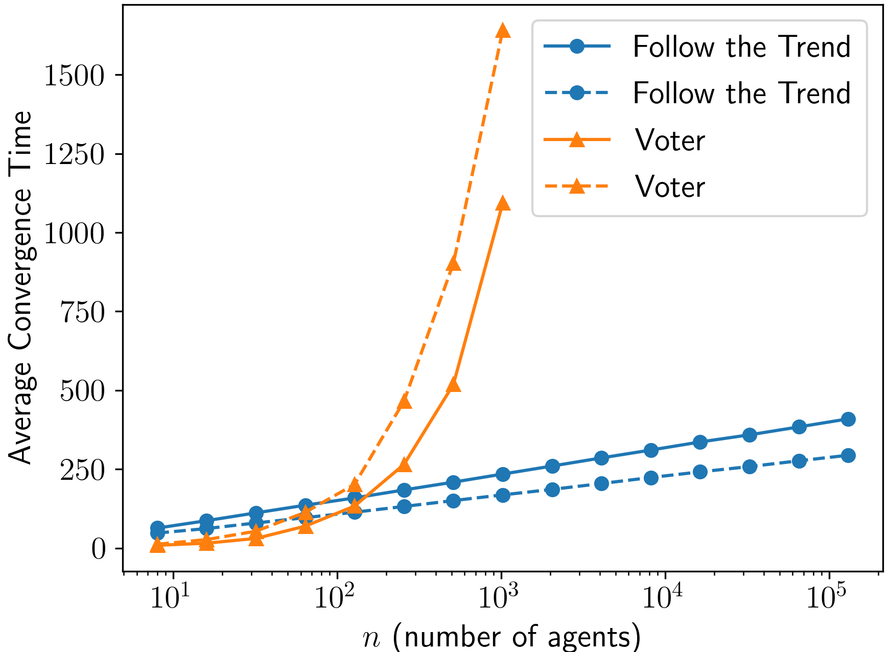
Simulations were performed for $n=2^{i}$, where $i\in\{3,\ldots,10\}$ for the Voter model, and $i\in\{3,\ldots,17\}$ for Algorithm 1, and repeated $100$ times each. Every population contains a single source agent ($z=1$). In self-stabilizing settings, it is not clear what are the worst initial configurations for a given dynamics. Here, we looked at two different ones:

• a configuration in which all opinions (including the one of the source agent) are independently and uniformly distributed in $\{0,1\}$,

• a configuration in which the source agent holds opinion $0$, while all other agents hold opinion $1$.

We compare it experimentally to the voter model. Simulations were performed for $n=2^{i}$, where $i\in\{3,\ldots,10\}$ for the voter model, and $i\in\{3,\ldots,17\}$ for our candidate dynamics, and repeated $100$ times each. Results are summed up in Figure 1, in terms of parallel rounds (one parallel round corresponds to $n$ activations). They suggest that convergence of our candidate dynamics takes about $\Theta(\mathrm{polylog}n)$ parallel rounds. In terms of parallel time, this represents an exponential gap when compared to the lower bound in Theorem 3 established for memoryless dynamics.

Figure 1: “Follow the Trend” versus the voter model. Average convergence time (in parallel rounds) is depicted for different values of $n$, over 100 iterations each, for $z=1$ source agent. Blue lines with circular markers correspond to our candidate dynamic which is an adaptation of the “follow the trend” algorithm from [14]. Orange lines with triangular markers correspond to the voter model. Full lines depict initial configurations in which all opinions are drawn uniformly at random from $\{0,1\}$. Dotted lines depict initial configurations in which all opinions are taken to be different from the source agent.

6 Discussion and Future Work

This work investigates the role played by memory in multi-agent systems that rely on passive communication and aim to achieve consensus on an opinion held by few “knowledgable” individuals [14, 3, 48]. Under the model we consider, we prove that incorporating past observations in the current decision is necessary for achieving fast convergence even if the observations regarding the current opinion configuration are complete. The same lower bound proof can in fact be adapted to any process that is required to alternate the consensus (or semi-consensus) opinion, i.e., to let the population agree (or almost agree) on one opinion, and then let it agree on the other opinion, and so forth. Such oscillation behaviour is fundamental to sequential decision making processes [48].

The ultimate goal of this line of research is to reflect on biological processes and conclude lower bounds on biological parameters. However, despite the generality of our model, more work must be done to obtain concrete biological conclusions. Conducting an experiment that fully adheres to our model, or refining our results to apply to more realistic settings remains for future work. Candidate experimental settings that appear to be promising include fish schooling [3, 17], collective sequential decision-making in ants [48], and recruitment in ants [18]. If successful, such an outcome would be highly pioneering from a methodological perspective. Indeed, to the best of our knowledge, a concrete lower bound on a biological parameter that is achieved in an indirect manner via mathematical considerations has never been obtained.

Acknowledgement.

The authors would like to thank Yoav Rodeh for very helpful discussions concerning the lower bound proof (Theorem 3).

References

- [1] David JT Sumpter. Collective animal behavior. In Collective Animal Behavior. Princeton University Press, 2010.
- [2] Ofer Feinerman and Amos Korman. Individual versus collective cognition in social insects. Journal of Experimental Biology, 220(1):73–82, 2017.
- [3] Iain D Couzin, Jens Krause, Nigel R Franks, and Simon A Levin. Effective leadership and decision-making in animal groups on the move. Nature, 433(7025):513–516, 2005.
- [4] Aviram Gelblum, Itai Pinkoviezky, Ehud Fonio, Abhijit Ghosh, Nir Gov, and Ofer Feinerman. Ant groups optimally amplify the effect of transiently informed individuals. Nature Communications, 6(1):1–9, 2015.
- [5] Ehud Fonio, Yael Heyman, Lucas Boczkowski, Aviram Gelblum, Adrian Kosowski, Amos Korman, and Ofer Feinerman. A locally-blazed ant trail achieves efficient collective navigation despite limited information. Elife, 5:e20185, 2016.
- [6] Lucas Boczkowski, Emanuele Natale, Ofer Feinerman, and Amos Korman. Limits on reliable information flows through stochastic populations. PLoS computational biology, 14(6):e1006195, 2018.
- [7] Ofer Feinerman and Amos Korman. The ants problem. Distributed Computing, 30(3):149–168, 2017.
- [8] William Bialek, Andrea Cavagna, Irene Giardina, Thierry Mora, Edmondo Silvestri, Massimiliano Viale, and Aleksandra M Walczak. Statistical mechanics for natural flocks of birds. Proceedings of the National Academy of Sciences, 109(13):4786–4791, 2012.
- [9] Richard M Karp. Understanding science through the computational lens. Journal of Computer Science and Technology, 26(4):569–577, 2011.
- [10] Brieuc Guinard and Amos Korman. Intermittent inverse-square lévy walks are optimal for finding targets of all sizes. Science Advances, 7(15):eabe8211, 2021.
- [11] James Aspnes and Eric Ruppert. An introduction to population protocols. Middleware for Network Eccentric and Mobile Applications, pages 97–120, 2009.
- [12] Lucas Boczkowski, Amos Korman, and Emanuele Natale. Minimizing message size in stochastic communication patterns: fast self-stabilizing protocols with 3 bits. Distributed Computing, 32(3), 2019.
- [13] Paul Bastide, George Giakkoupis, and Hayk Saribekyan. Self-stabilizing clock synchronization with 1-bit messages. In ACM-SIAM Symposium on Discrete Algorithms, pages 2154–2173. SIAM, 2021.
- [14] Amos Korman and Robin Vacus. Early adapting to trends: Self-stabilizing information spread using passive communication. In ACM Symposium on Principles of Distributed Computing, pages 235–245. ACM, 2022.
- [15] Nigel R Franks, Stephen C Pratt, Eamonn B Mallon, Nicholas F Britton, and David JT Sumpter. Information flow, opinion polling and collective intelligence in house–hunting social insects. Philosophical Transactions of the Royal Society of London. Series B: Biological Sciences, 357(1427):1567–1583, 2002.
- [16] M Lindauer. Communication in swarm-bees searching for a new home. Nature, 179(4550):63–66, 1957.
- [17] Iain D Couzin, Christos C Ioannou, Güven Demirel, Thilo Gross, Colin J Torney, Andrew Hartnett, Larissa Conradt, Simon A Levin, and Naomi E Leonard. Uninformed individuals promote democratic consensus in animal groups. Science, 334(6062):1578–1580, 2011.
- [18] Nitzan Razin, Jean-Pierre Eckmann, and Ofer Feinerman. Desert ants achieve reliable recruitment across noisy interactions. Journal of the Royal Society Interface, 10(82):20130079, 2013.
- [19] Thomas D Seeley. Consensus building during nest-site selection in honey bee swarms: the expiration of dissent. Behavioral Ecology and Sociobiology, 53(6):417–424, 2003.
- [20] Gerald S Wilkinson. Information transfer at evening bat colonies. Animal Behaviour, 44:501–518, 1992.
- [21] Noam Cvikel, Katya Egert Berg, Eran Levin, Edward Hurme, Ivailo Borissov, Arjan Boonman, Eran Amichai, and Yossi Yovel. Bats aggregate to improve prey search but might be impaired when their density becomes too high. Current Biology, 25(2):206–211, 2015.
- [22] Luc-Alain Giraldeau and Thomas Caraco. Social foraging theory. In Social Foraging Theory. Princeton University Press, 2018.
- [23] Grant Schoenebeck and Fang-Yi Yu. Consensus of interacting particle systems on erdös-rényi graphs. In Proceedings of the Twenty-Ninth ACM-SIAM Symposium on Discrete Algorithms, pages 1945–1964, 2018.
- [24] Artur Czumaj and Andrzej Lingas. On parallel time in population protocols. Information Processing Letters, 179:106314, 2023.
- [25] Alan Demers, Dan Greene, Carl Hauser, Wes Irish, John Larson, Scott Shenker, Howard Sturgis, Dan Swinehart, and Doug Terry. Epidemic algorithms for replicated database maintenance. In 6th ACM Symposium on Principles of Distributed Computing, pages 1–12, 1987.
- [26] Richard Karp, Christian Schindelhauer, Scott Shenker, and Berthold Vocking. Randomized rumor spreading. In 41st IEEE Symposium on Foundations of Computer Science, pages 565–574, 2000.
- [27] Michael Ben-Or, Danny Dolev, and Ezra N Hoch. Fast self-stabilizing byzantine tolerant digital clock synchronization. In 27th ACM symposium on Principles of Distributed Computing, pages 385–394, 2008.
- [28] Dana Angluin, James Aspnes, Zoë Diamadi, Michael J Fischer, and René Peralta. Computation in networks of passively mobile finite-state sensors. In Twenty-third ACM symposium on Principles of Distributed Computing, pages 290–299, 2004.
- [29] Luca Becchetti, Andrea E. F. Clementi, and Emanuele Natale. Consensus dynamics: An overview. SIGACT News, 51(1):58–104, 2020.
- [30] Adam Coates, Liangxiu Han, and Anthony Kleerekoper. A unified framework for opinion dynamics. In 17th International Conference on Autonomous Agents and MultiAgent Systems, AAMAS 2018, pages 1079–1086, 2018.
- [31] Charlotte Out and Ahad N. Zehmakan. Majority vote in social networks: Make random friends or be stubborn to overpower elites. In 30th International Joint Conference on Artificial Intelligence, pages 349–355, 2021.
- [32] Peter Clifford and Aidan Sudbury. A model for spatial conflict. Biometrika, 60(3):581–588, 1973.
- [33] Richard A Holley and Thomas M Liggett. Ergodic theorems for weakly interacting infinite systems and the voter model. The Annals of Probability, pages 643–663, 1975.
- [34] P. L. Krapivsky and S. Redner. Dynamics of majority rule in two-state interacting spin systems. Phys. Rev. Lett., 90:238701, 2003.
- [35] Petra Berenbrink, Martin Hoefer, Dominik Kaaser, Pascal Lenzner, Malin Rau, and Daniel Schmand. Asynchronous opinion dynamics in social networks. In 21st International Conference on Autonomous Agents and Multiagent Systems, pages 109–117, 2022.
- [36] Benjamin Doerr, Leslie Ann Goldberg, Lorenz Minder, Thomas Sauerwald, and Christian Scheideler. Stabilizing consensus with the power of two choices. In 23rd ACM Symposium on Parallelism in Algorithms and Architectures, 2011.
- [37] Elchanan Mossel, Joe Neeman, and Omer Tamuz. Majority dynamics and aggregation of information in social networks. Auton. Agents Multi Agent Syst., 28(3):408–429, 2014.
- [38] Aris Anagnostopoulos, Luca Becchetti, Emilio Cruciani, Francesco Pasquale, and Sara Rizzo. Biased opinion dynamics: When the devil is in the details. In 29th International Joint Conference on Artificial Intelligence, pages 53–59, 2020.
- [39] Emilio Cruciani, Hlafo Alfie Mimun, Matteo Quattropani, and Sara Rizzo. Phase transitions of the k-majority dynamics in a biased communication model. In ACM International Conference on Distributed Computing and Networking, pages 146–155. ACM, 2021.
- [40] Hicham Lesfari, Frédéric Giroire, and Stéphane Pérennes. Biased majority opinion dynamics: Exploiting graph k-domination. In 31st International Joint Conference on Artificial Intelligence, pages 377–383. ijcai.org, 2022.
- [41] Francesco D’Amore, Andrea E. F. Clementi, and Emanuele Natale. Phase transition of a nonlinear opinion dynamics with noisy interactions. Swarm Intell., 16(4):261–304, 2022.
- [42] Naoki Masuda. Opinion control in complex networks. New Journal of Physics, 17, 03 2015.
- [43] Guillermo Romero Moreno, Long Tran-Thanh, and Markus Brede. Continuous influence maximisation for the voter dynamics: is targeting high-degree nodes a good strategy? In International Conference on Autonomous Agents and Multi-Agent Systems, 2020.
- [44] Ercan Yildiz, Asuman Ozdaglar, Daron Acemoglu, Amin Saberi, and Anna Scaglione. Binary opinion dynamics with stubborn agents. ACM Trans. Econ. Comput., 1(4), dec 2013.
- [45] Mikaela Irene D Fudolig and Jose Perico H Esguerra. Analytic treatment of consensus achievement in the single-type zealotry voter model. Physica A: Statistical Mechanics and its Applications, 413:626–634, 2014.
- [46] Thomas Milton Liggett. Interacting particle systems, volume 276. Springer Science & Business Media, 2012.
- [47] David A Levin and Yuval Peres. Markov chains and mixing times, volume 107. American Mathematical Soc., 2017.
- [48] Oran Ayalon, Yigal Sternklar, Ehud Fonio, Amos Korman, Nir S Gov, and Ofer Feinerman. Sequential decision-making in ants and implications to the evidence accumulation decision model. Frontiers in applied mathematics and statistics, page 37, 2021.