THC: Accelerating Distributed Deep Learning Using Tensor Homomorphic Compression

Abstract.

Deep neural networks (DNNs) are the de-facto standard for essential use cases, such as image classification, computer vision, and natural language processing. As DNNs and datasets get larger, they require distributed training on increasingly larger clusters. A main bottleneck is then the resulting communication overhead where workers exchange model updates (i.e., gradients) on a per-round basis. To address this bottleneck and accelerate training, a widely-deployed approach is compression. However, previous deployments often apply bi-directional compression schemes by simply using a uni-directional gradient compression scheme in each direction. This results in significant computational overheads at the parameter server and increased compression error, leading to longer training and lower accuracy.

We introduce Tensor Homomorphic Compression (THC), a novel bi-directional compression framework that enables the direct aggregation of compressed values while optimizing the bandwidth to accuracy tradeoff, thus eliminating the aforementioned overheads. Moreover, THC is compatible with in-network aggregation (INA), which allows for further acceleration. Evaluation over a testbed shows that THC improves time-to-accuracy in comparison to alternatives by up to 1.32$\times$ with a software PS and up to 1.51$\times$ using INA. Finally, we demonstrate that THC is scalable and tolerant for acceptable packet-loss rates.

1. Introduction

In the past decade, the scale of machine learning training and data volume has increased dramatically due to the growing demand for various ML applications (Redmon et al., 2016; Cohen et al., 2022; Brown et al., 2020; Simonyan and Zisserman, 2014; He et al., 2016; Wang and O’Boyle, 2018; Wang et al., 2016; Wu et al., 2016). For example, Nvidia’s Megatron-LM (Narayanan et al., 2021) required 3072 GPUs across 384 machines to train. Alibaba’s general-purpose ML platforms also reported a rapid increase in ML training data, from hundreds of gigabytes to tens or even hundreds of terabytes, at an internet scale, within a few years (Weng et al., 2022). This trend is expected to continue in the future (Sevilla et al., 2022) with the rapid advancements of MoE (Mixture of experts)  (Shazeer et al., 2017; Rajbhandari et al., 2022) and other giant models (Cohen et al., 2022; Brown et al., 2020; Naumov et al., 2019). To support these large-scale models, we need large-scale distributed training, which incurs more network communications.

Meanwhile, hardware computing has made great strides in recent years (Jouppi et al., 2017). The advent of specialized ML accelerators (Fowers et al., 2018; vit, 2023; McDanel et al., 2019; Petrica et al., 2020) and the advancements in GPU/TPU hardware have improved the training efficiency significantly. Such increasing computing power generates higher throughput traffic into the network. Yet, the communication cost rises as the number of computing devices (workers) increases. To handle this massive data volume, compression is widely used to reduce communication cost (Bai et al., 2021; Wang et al., 2023). However, compression comes with extra computation costs and may affect training convergence and attainable accuracy.

For example, with the parameter server (PS) architecture, where workers may send their compressed model updates (i.e., gradients) to the PS at each round, the PS must first decompress all gradients, aggregate them, and then compress the aggregated gradients again. Our microbenchmark shows that in a 4 workers 1 PS setting with TopK 5% compression, the compression overhead can account for up to 51.45% of the total round time (Fig. 2(b)). Moreover, inaccurate and compute-intensive compression may negatively impact overall training performance because it may both prolong round time and the number of rounds it takes to reach the target accuracy. For example, Espresso (Wang et al., 2023) shows that training an LSTM model using DGC compression with a 1% compression rate (i.e., 100$\times$ bandwidth reduction) can slow down overall performance by up to 9%.

We observe that the main problem with such previous deployments is that they often apply bi-directional compression schemes by simply using a uni-directional gradient compression scheme in each direction, resulting in significant computational overheads at the parameter server and increased compression error, leading to longer training times and lower resulting model accuracy.

To address these problems, we introduce Tensor Homomorphic Compression (THC), a novel bi-directional compression framework that enables the direct aggregation of compressed values while optimizing the bandwidth to accuracy tradeoff, thus eliminating the aforementioned overheads. Moreover, THC is compatible with in-network aggregation (INA), which allows for further acceleration. A key idea behind THC is to leverage minimal information exchange between the workers at the beginning of each communication stage to coordinate their compression, which allows for accurate aggregation in compressed form.

We showcase the benefits of THC by implementing a software PS and a worker compression module within the BytePS (Jiang et al., 2020) PyTorch extension. We also incorporate it into in-network aggregation services (Sapio et al., 2021; Lao et al., 2021; Gebara et al., 2021), which employ programmable switches to perform gradient aggregation.

We perform extensive evaluation over seven representative DNN models on a single rack testbed with four workers, a programmable switch, and 100 Gbps network. Our experiment result demonstrates that THC improves training throughput by up to 85% and outperforms state-of-the-art distributed training framework (BytePS) in terms of time-to-target-accuracy by 63%. We also simulate multi-worker scenarios to show that THC scales well, tolerates packet loss, and offers new opportunities for partial aggregation and straggler handling. This work does not raise any ethical issues.

2. Background and Motivation

In this section, we discuss the network bottleneck in distributed training and overview two key solutions for reducing bandwidth: compression and in-network aggregation.

2.1. Network bottleneck in DNN training

As the size of machine learning models and datasets increases, distributed training across multiple machines becomes an efficient way to accelerate training. In practical data parallelism, two popular architectures for distributed learning are Parameter Server (PS) (Li et al., 2014) and AllReduce (Patarasuk and Yuan, 2009). In AllReduce, all workers perform aggregation and broadcast without needing dedicated servers for coordination. In the PS architecture, workers send their gradients to the PS that aggregates them, usually by averaging, and sends the result back to the workers. While all-reduce architecture gains much attention, the PS architecture has been proven to be effective in a GPU/CPU heterogeneous setting (Jiang et al., 2020), which is common in cloud environments that have spare CPU resources (Jeon et al., 2019). A series of works have followed this line, making progress in PS architecture research (Jiang et al., 2020; Wang et al., 2023; Peng et al., 2019). Indeed, in this paper, we focus on the PS architecture but discuss how our schemes can be used for AllReduce in Section 10.

Nowadays, both AllReduce and PS architecture incur high communication overhead. Recent research (Wang et al., 2023) has shown that the synchronization cost of GPT2 (Radford et al., 2019) and BERT-base (Devlin et al., 2018) in a 8-worker setting can be as high as 42% and 49% of the total time during training even with state-of-the-art frameworks. As the number of participating workers increases, there is a substantial increase in communication costs expected (Sevilla et al., 2022). Moreover, computing performance is growing at a faster pace than inter-machine bandwidth (Sun et al., 2019; Zhou et al., 2020), particularly with the emergence of new hardware solutions such as TPUs. This will further increase the network bottleneck.

A straightforward solution to mitigate the communication overhead is increasing the batch size and hence bringing down the synchronization frequency. Unfortunately, previous studies have shown that this approach has diminishing returns (Keskar et al., 2017). GPU memory also imposes a constraint on the maximum batch size a node can use.

2.2. Compression

A well-studied approach to reducing the network bottleneck of distributed training is gradient compression. Gradient compression allows one to reduce the volume of gradients transmitted in synchronization steps through sparsification and/or quantization. For example, sparsification may filter out coordinates of small magnitude in the gradient tensor before sending it out. TopK (Stich et al., 2018) is a straightforward sparsification algorithm, which only sends the top $k$ percent (by magnitude) of coordinates in a gradient tensor and their indices. Quantization reduces the size of each element by reducing the precision of gradients. For example, TernGrad(Wen et al., 2017) reduces the bit length of the gradient coordinates to two bits by converting each float into a value $x\in\{-1,0,1\}$.

Figure 1 shows the bi-directional compression process in existing PS architecture systems (Bai et al., 2021; Wang et al., 2023). The workers send compressed gradients to the PS, which decompresses and then aggregates them. Then to reduce the traffic from the PS back to the workers, we need to compress the aggregated results again at the PS.

While compression reduces the communication cost, decompressing and compressing data on PS nodes can introduce non-negligible compute overhead and additional compression error. Figure 2(b) shows a microbenchmark experiment on a testbed with four workers (see Section 8 for details), which measures the worker side compression and decompression time (”worker compression overhead”), communication time, the PS side compression and decompression time (”PS compression overhead”), and the PS summation time when communicating a vector with one million coordinates. Compared with the baseline without compression, TopK 10% reduces the communication time by 1.83 ms but takes an extra 3.86 ms to run compression/decompression at the PS side. TopK 5% shows similar numbers with 3.86 ms less communication time but 3.88 ms more PS compression time compared to no compression. The PS overhead is expected to become larger as the number of workers increases, or when the worker-to-parameter server ratio is imbalanced, causing each parameter server to serve multiple machines.

One can use other compression schemes (e.g., TernGrad) that take less time for decompression/compression at the PS side. However, these schemes have a significantly larger quantization error. Figure 2(b) shows the NMSE (Normalized Mean Squared Error, which quantifies the difference between the actual vector and the vector restored after compression; smaller is better) for different compression algorithms. Terngrad results in an NMSE that is by almost two orders of magnitude larger than that of TopK 10% (i.e., 15.7 vs. 0.36 with 2 workers). This large gap in NMSE means that Terngrad may require more iterations to reach the target accuracy or fail to reach the target accuracy at all. In fact, provable convergence rates for distributed SGD have a linear dependence on NMSE (e.g., (Karimireddy et al., 2019)), rendering quantization schemes with large NMSE less appealing for distributed training. To address these limitations, THC eliminates decompression-compression at the PS with negligible impact on accuracy.

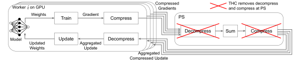
Figure 1. End-to-end workflow when using typical compression algorithms.

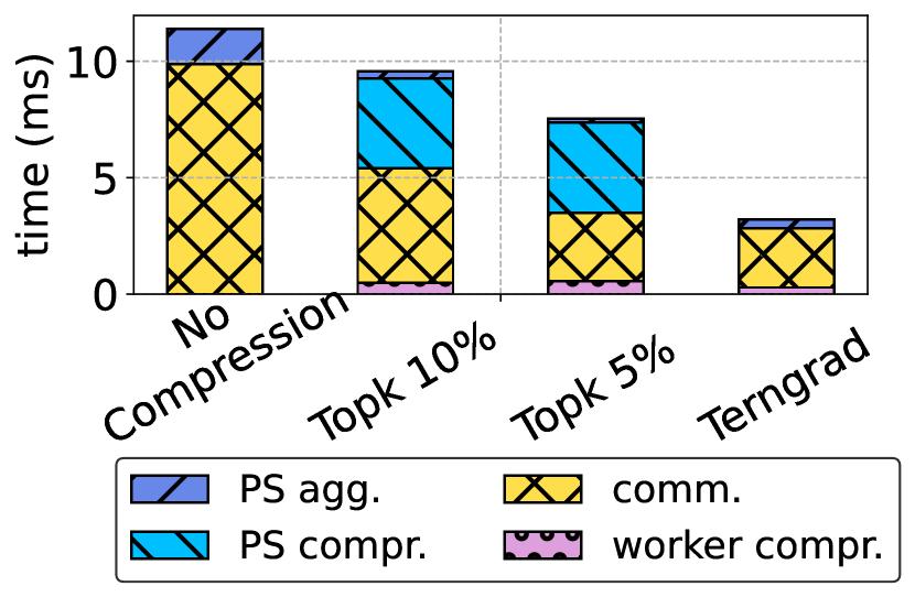
(a) Communication round time, 4 workers + 1 PS.

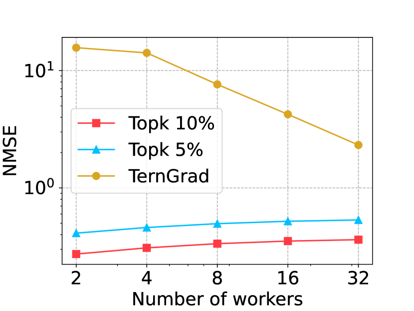
(b) NMSE of different compression algorithms.

Figure 2. Communication time and error.

2.3. In-network aggregation

In-network aggregation (NVI, 2020) is another option to reduce network bottlenecks by using switches. Recent research (Sapio et al., 2021) has demonstrated that programmable switches can aggregate gradients from multiple workers, reducing the switch-to-PS traffic and resulting in a substantial training performance improvement. However, the traffic generated by the workers is of equal amount and cannot be reduced by switches.

Current in-network aggregation approaches do not consider compression, because compressed data can not be easily aggregated without decompressing in the network. Meanwhile, implementing such decompression and aggregation functions in the specialized hardware is extremely difficult given the restricted programmability of such hardware. For example,  (Lao et al., 2021; Ports and Nelson, 2019) reported that the hardware has very limited pipeline stages (around 10 to 20) to do fixed-function operations such as modifying packet values.

However, with THC, in-network aggregation is freed from considering additional design considerations for compression. In addition, by offloading computation to programmable hardware, we can further reduce the PS time overhead.

We leverage THC’s attributes of homomorphic aggregation in the framework to offer new opportunities for incorporating compression with in-network aggregation without complex coding efforts, making these two components complement each other perfectly.

3. THC Overview

As mentioned in Section 2.1, in distributed DNN training, at each round, each worker computes a local gradient, and the model’s weights are updated using the average of the workers’ gradients (or an estimate thereof). Our goal is then to allow the workers to accurately estimate the gradients’ average while minimizing the associated overheads. Accordingly, we propose the Tensor Homomorphic Compression (THC) framework, which supports direct gradient aggregation of compressed gradients. Consider $n$ workers and let $\nabla_{i}$ be the worker’s $i$ gradient. THC relies on a new compression scheme that satisfies the following property:

Definition 0 (Uniform Homomorphic Compression).

$$\widehat{\nabla}_{\mathit{avg}}=\frac{1}{n}\cdot\sum_{i}\texttt{Decompress}(\texttt{Compress}(\nabla_{i}))=\\ \texttt{Decompress}\left(\frac{1}{n}\cdot\sum_{i}\texttt{Compress}(\nabla_{i})\right).$$

That is, in Uniform Homomorphic Compression (UHC), the average of the decompressed gradients is mathematically equivalent to decompressing the average compressed gradient. Leveraging this property, the PS simply sums the compressed gradients and sends the result back (still in compressed form). Finally, each worker averages the result and applies the decompression to derive the update $\widehat{\nabla}_{avg}$.

This process is visualized in Fig. 3. It starts by having worker $i$ compress its gradient, which commonly consists of $32$-bit floats. Namely, each coordinate is encoded using a table index that requires a small number of bits, e.g., $4$. The table indices are then packed and sent to the PS, resulting in a significant bandwidth reduction, i.e., $\times 8$ in our example. The PS then looks the table indices up in a lookup table to receive the corresponding table values. The table serves two purposes: first, it allows an efficient expansion of the indices to wider values, e.g., of $8$-bits each, that allow summation without overflows. Second, we can use the table to minimize the quantization error, as we later show, by picking the table values in correspondence to the underlying data distribution. The PS sums up the looked-up table values coordinate-wise, packs the result, and broadcasts it to the workers. In our example, this results in a $\times 4$ bandwidth reduction in this direction without any additional quantization error or decompression delay at the PS. Finally, each worker decompresses and normalizes the result to obtain the average gradient’s estimate.

The key challenge for THC is how to support the aggregation of compressed gradients while minimizing the impact on accuracy. Previous compression techniques require the PS to decompress the gradients before aggregation because they rely only on worker-local information. When workers use different quantization ranges (e.g., (Alistarh et al., 2017; Ramezani-Kebrya et al., 2021)), the PS must decompress each gradient separately, sum them up, and compress again, increasing processing delay at the PS side and the errors caused by compression. Or we can rely on biased quantization (e.g., (Bernstein et al., 2018)), but these approaches introduce even larger errors in compression.

In THC, we retain an accuracy that is similar to that of the uncompressed baseline. Intuitively, this is because THC’s quantization error adds variance to the estimate of the average gradient that is smaller than that of the inherent variance in distributed SGD. Namely, we optimize the bandwidth-accuracy tradeoff and pick an operating point in which the estimation accuracy is sufficient.

To summarize, traditional bi-directional compression approaches require the PS to perform $n$ decompression operations in order to aggregate the gradients before recompressing them and introducing an additional error. Instead, in THC, the PS simply sums up the looked-up table values coordinate-wise and broadcasts them back to the workers without any additional error. In turn, each of the $n$ workers makes a single decompression in parallel, thereby accelerating the process.

Next, we present the THC framework in detail in Section 4; in Section 5, we introduce further optimizations for THC and the end-to-end training procedure; then, Section 6 shows how THC can be seamlessly used in conjunction with in-network aggregation to further accelerate the training.

4. ​ Tensor Homomorphic Compression

A main building block that is used for gradient compression is quantization, a technique that allows representing gradient entries (e.g., 32-bit floats) using a small (e.g., 4) number of bits while bounding the error. At a high level, our Tensor Homomorphic Compression (THC) framework leverages the concept of Stochastic Quantization (SQ) that quantizes given a real-value $a$ to one of two quantization values $q_{0},q_{1}$ such that $q_{0}\leq a\leq q_{1}$. SQ quantizes $a$ to $q_{1}$ with probability $(q_{1}-a)/(q_{1}-q_{0})$ and to $q_{1}$ otherwise. An appealing property of SQ is that the expected value of the quantization is exactly $a$, i.e., it is unbiased. This is especially useful in distributed scenarios where using SQ results in a decrease in the error of estimating the average as the number of workers increases (Vargaftik et al., 2021).

The most popular form of SQ is Uniform SQ (USQ) in which the quantization values are uniformly spaced. For example, given the range $[m,M]$ and using $2^{b}$ quantization values, their locations are $q_{0}=m,q_{1}=m+(M-m)/(2^{b}-1),\ldots,q_{2^{b}}=M$. USQ quantizes a value $a\in[m,M]$ to one of its nearest quantization values.

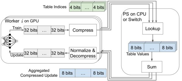
Figure 3. THC’s workflow illustration.

4.1. The Uniform THC algorithm

To develop THC, we first introduce a generalization of USQ to the uniform homomorphic setting. For convenience, we henceforth denote $\left\langle i\right\rangle=\left\{0,\ldots,i-1\right\}$ for any $i\in\mathbb{N}$.

Definition 0 (Homomorphic USQ).

Let $\nabla_{0},\nabla_{1},\ldots,\nabla_{n-1}\in\mathbb{R}^{d}$ be the input gradients, and let $m_{i}=\min\left\{\nabla_{i}\right\}$ and $M_{i}=\max\left\{\nabla_{i}\right\}$ be the $i$’th gradient’s minimum and maximum. Let $m=\min_{i}\left\{m_{i}\right\}$ and $M=\max_{i}\left\{M_{i}\right\}$ and consider a set of uniformly spaced quantization values $\left\{m+k\cdot\frac{M-m}{2^{b}-1}\mid k\in\left\langle 2^{b}\right\rangle\right\}$. The workers perform stochastic quantization using these quantization values on all input gradients.

This approach is homomorphic (Definition 3.1) since ($C$ and $D$ stand for Compress and Decompress):

$$\frac{1}{n}\cdot\sum_{i\in\left\langle n\right\rangle}D(C(\nabla_{i}))=\frac{1}{n}\cdot\sum_{i\in\left\langle n\right\rangle}\left(m+C(\nabla_{i})\cdot\frac{M-m}{2^{b}-1}\right)\\ =m+\left(\frac{1}{n}\cdot\sum_{i\in\left\langle n\right\rangle}C(\nabla_{i})\right)\cdot\frac{M-m}{2^{b}-1}=D\left(\frac{1}{n}\cdot\sum_{i\in\left\langle n\right\rangle}C(\nabla_{i})\right).$$

With this primitive at hand, we are ready to introduce a simplified (uniform) variant of the THC framework (which we later generalize to a non-uniform setting).

The pseudo-code of Uniform THC is given by Algorithm 1. It begins with a preliminary communication round where each worker computes and sends the smallest and largest gradient entry to the PS (lines 6-7). In turn, the PS computes the extreme global values and distributes them back to the workers (lines 9-10). This communication round is light and requires each worker to transmit and receive only two floats. Next, each worker quantizes its gradient using the global extremes (i.e., perform Homomorphic USQ) and sends the result to the PS (lines 15-16). Then, the PS sums all the quantized vectors and sends their sum to the worker (lines 18-19). Finally, each worker divides the sum by the number of workers to obtain the estimate of the average (line 21).

As detailed in Section 5, we can reduce the quantization error by pre-processing the input gradient prior to its quantization and post-processing the average’s estimate at the end.

Algorithm 1 Uniform THC

1: Input: bit budget $b$

2:

3:   Preliminary stage

4:

5:Worker $i$:

6:Compute $m_{i}=\min\left\{\nabla_{i}\right\}$ and $M_{i}=\max\left\{\nabla_{i}\right\}$

7:Send $(m_{i},M_{i})$ to the PS

8:PS:

9:Compute $m=\min_{i}\left\{m_{i}\right\}$ and $M=\max_{i}\left\{M_{i}\right\}$

10:Send $(m,M)$ to workers

11:

12:   Main stage

13:

14:Worker $i$:

15:Compute $X_{i}=\mathit{USQ}(\nabla_{i},m,M,b)$

16:Send $X_{i}$ to PS

17:PS:

18:Compute $X=\sum_{i\in\left\langle n\right\rangle}X_{i}$

19:Send $X$ to workers

20:Worker $i$:

21:Estimate $\widehat{\nabla}_{\mathit{avg}}=m+\frac{1}{n}\cdot X\cdot\frac{M-m}{2^{b}-1}$

4.2. The Non-uniform THC algorithm

In many cases, it is possible to choose the quantization values in a non-uniform manner to optimize the accuracy-bandwidth tradeoff. However, it is unclear how to leverage existing non-uniform quantization methods (e.g.,  (Ramezani-Kebrya et al., 2021; Suresh et al., 2017; Vargaftik et al., 2022)) to improve our homomorphic compression. Namely, in non-uniform methods, the sender transmits a table index $z$ that is then converted to the table value $T[z]$ by the receiver. Here, $T$ is a lookup table that converts indices to values that may not be uniformly spaced, i.e., $T[z+1]-T[z]$ may not equal $T[z^{\prime}+1]-T[z^{\prime}]$ for different indices $z,z^{\prime}$.

For example, consider quantizing values in the range $[-1,1]$ using four quantization values. Using USQ, the lookup table is $T[0]=-1,T[1]=-1/3,T[2]=1/3,T[3]=1$. In this case, any sum of table indices corresponds to a single sum of quantization values. For example, suppose two senders send indices $z,z^{\prime}$ and consider two cases: (1) $z=0,z^{\prime}=3$ and (2) $z=1,z^{\prime}=2$. In both cases, $T[z]+T[z^{\prime}]=0$. That is, $z+z^{\prime}=3$ implies that $T[z]+T[z^{\prime}]=0$. Intuitively, the receiver can sum the indices and deduce the sum of sent values instead of performing two table lookups.

In contrast, consider non-uniform quantization that uses the table $T[0]=-1,T[1]=-1/2,T[2]=1/2,T[3]=1$. Consider the two cases in which $z+z^{\prime}=4$: (1) $z=1,z^{\prime}=3$ and (2) $z=z^{\prime}=2$. In the first case, $T[z]+T[z^{\prime}]=1/2$ while in the second $T[z]+T[z^{\prime}]=1$. That is, the sum of table indices does not determine the sum of table values, and thus, the receiver lookup each index individually.

Our insight is that we can overcome this by mapping each message to a different representation that is homomorphically aggregable. To that end, for a bit-budget of $b$ bits per coordinate, we define a hyperparameter $g\geq 2^{b}-1$ called granularity. We then use a table $T:\left\langle 2^{b}\right\rangle\to\left\langle g+1\right\rangle$ that maps table indices to values that are integers in the larger range. Intuitively, one can think about this as running USQ with $g+1$ quantization values, but where senders are only allowed $2^{b}$ indices. A table value $T[z]$ then corresponds to the quantization value $m+T[z]\cdot\frac{M-1}{g+1}$, same as in USQ. For instance, in the above example, the PS can use a table $T[0]=0,T[1]=1,T[2]=3,T[3]=4$ to map each table index into (the larger) range $\left\langle 5\right\rangle$. The benefit is that the table values are now directly aggregable; for example, consider three senders with the two cases (1) $z=0=z^{\prime}=z^{\prime\prime}=1$ and thus $T[z]=T[z^{\prime}]=T[z^{\prime\prime}]=1$, i.e., all quantization values are $-1/2$; (2) $z=z^{\prime}=0,z^{\prime\prime}=2$ and thus $T[z]=T[z^{\prime}]=0,T[z^{\prime\prime}]=3$, i.e., the first two quantization values are $-1$ and the third is $1/2$. Notice that the sum of table values is the same in both cases, and so is the sum of quantization values; in contrast, the sum of table indices differ.

Intuitively, $g$ introduces a tradeoff where larger $g$ results in a more fine-grained choice of quantization values and lower error, but it also requires more bits to represent the summation and higher bandwidth requirement from the PS or switch to the workers.

The pseudocode for the non-uniform variant of THC appears in Algorithm 2 (the Preliminary stage is the same as in Algorithm 1). Notice that the lookup table $T_{b,g}$ depends on bit-budget $b$ and the granularity $g$. When clear from context, we omit the subscripts and write $T$.

Each worker $i$ then calculates the set of quantization values $Q\subset[m,M]$ given the (global) $m,M$ and the granularity $g$ (7). Next, it stochastically quantizes each coordinate to a value in $Q$, giving the result $X_{i}\in Q^{d}$ (8). The worker then transforms each quantized coordinate into its uniform-HC value in $\left\langle g+1\right\rangle$ using the linear transformation (9). The next stage involves computing which $b$-bit table indices (in $\left\langle 2^{b}\right\rangle$) would map to the uniformly partitioned values by applying the inverse mapping (10). Finally, it sends the result $Z_{i}$ to the PS (11).

The PS then gets the set of vectors $\left\{Z_{i}\right\}_{i\in\left\langle n\right\rangle}$. It looks up each vector (coordinate-wise) and sums them up, corresponding to the sum of the $Y_{i}$’s (13). Then, the PS sends the result, $Y$, to the workers, still in compressed form (14). Observe that the PS only performs table lookups followed by summation without decompressing the vectors and without any additional processing and re-compression that increases the estimation error.

The final part takes place in parallel, where each worker $i$ first computes the average of $\sum_{i\in\left\langle n\right\rangle}Y_{i}$ by dividing $Y$ by $n$ (16). It then applies the inverse transformation to 9 to obtain an estimate $\widehat{\nabla}_{\mathit{avg}}$ of the average gradient (17).

To show that our algorithm is homomorphic, we generalize Definition 3.1 to account for the lookup table ($C,D$ and $T$ stand for Compress, Decompress and table lookup)

Definition 0 (Non-uniform homomorphic compression).

$$\widehat{\nabla}_{\mathit{avg}}=\frac{1}{n}\cdot\sum_{i\in\left\langle n\right\rangle}D(T(C(\nabla_{i})))=D\left(\frac{1}{n}\cdot\sum_{i\in\left\langle n\right\rangle}T(C(\nabla_{i}))\right).$$

That is, a non-uniform HC (NUHC) scheme generalizes UHC by allowing the PS to apply a lookup table $T$ to the compressed gradients before aggregating them.

Notice that if $g=2^{b}-1$ and $T$ is the identity mapping, NUHC is identical to UHC (in that case, the lookup table is redundant). As shown above, for $T$ that is the identity mapping, the compression is uniform homomorphic. We now show that if $0=T(0)<T(1)<\ldots<T(2^{b}-1)=g$ then Algorithm 2 is homomorphic. This is because

$$\frac{1}{n}\cdot\sum_{i\in\left\langle n\right\rangle}D(T(C(\nabla_{i})))=\frac{1}{n}\cdot\sum_{i\in\left\langle n\right\rangle}D(T(Z_{i}))=\\ \frac{1}{n}\cdot\sum_{i\in\left\langle n\right\rangle}D(Y_{i})=\frac{1}{n}\cdot\left(\sum_{i\in\left\langle n\right\rangle}m+Y_{i}\cdot\frac{M-m}{g}\right)=\\ m+\left(\frac{1}{n}\cdot\sum_{i\in\left\langle n\right\rangle}Y_{i}\right)\cdot\frac{M-m}{g}=D\left(\frac{1}{n}\cdot\sum_{i\in\left\langle n\right\rangle}T(C(\nabla_{i}))\right)\ ,$$

where we used (i) $C(\nabla_{i})=Z_{i}$, (ii) $T(C(\nabla_{i}))=T_{b,g}[Z_{i}]=Y_{i}$, and (iii) $D(Y_{i})=m+Y_{i}\cdot\frac{M-m}{g}$.

The above result shows that Algorithm 2 is homomorphic for many choices of lookup tables. As we later demonstrate, very small lookup tables (e.g., for $b=4$ we can usually use $g\in\left\{16,\ldots,51\right\}$) are sufficient to obtain accurate quantization.

Algorithm 2 Non-uniform THC

1: Input: bit budget $b$, granularity $g$, and their lookup-table $T_{b,g}$

2:

3:

4:   Main stage $\triangleright$  Preliminary stage same as in Algorithm 1

5:

6:Worker $i$:

7:Compute $Q=\mathit{CalcQuantizationValues}(m,M,T_{b,g})$

8:Compute $X_{i}=\mathit{SQ}(\nabla_{i},Q)$

9:Compute $Y_{i}=(X_{i}-m)\cdot\frac{g}{M-m}$ $\triangleright$  $Y_{i}\in\left\langle g+1\right\rangle^{d}$

10:Compute $Z_{i}=T_{b,g}^{-1}[Y_{i}]$$\triangleright$   $Z_{i}\in\left\langle 2^{b}\right\rangle^{d}$

11:Send $Z_{i}$ to PS

12:PS:

13:Compute $Y=\sum_{i\in\left\langle n\right\rangle}T_{b,g}[Z_{i}]$$\triangleright$  $Y\in\left\langle g\cdot n+1\right\rangle^{d}$

14:Send $Y$ to workers

15:Worker $i$:

16:Compute $Y_{\mathit{avg}}=\frac{1}{n}\cdot Y$$\triangleright$  $Y_{\mathit{avg}}\in[0,g]^{d}$

17:Estimate $\widehat{\nabla}_{\mathit{avg}}=m+Y_{\mathit{avg}}\cdot\frac{M-m}{g}$

5. Optimizing THC

In this section, we describe several optimizations that improve THC’s bandwidth-accuracy tradeoff.

5.1. Pre- and post-processing

A key quantity that determines the error of a quantization scheme is its range (the difference between the largest and smallest quantization values), $M-m$ (see Section A.2 for more details). Intuitively, when the range is large, one is forced to quantize to values that are further away from the encoded quantity, thus increasing the error. We describe two complementary methods for reducing it. Both methods reduce the estimation error by pre-processing the input gradient prior to its quantization and post-processing the average’s estimate at the end.

Transform.

We utilize the Randomized Hadamard Transform (RHT) as pre-processing, which is known to decrease the expected range. The RHT of a vector $x\in\mathbb{R}^{d}$ is defined as $H\cdot D\cdot x$, where $H$ is the Hadamard matrix (Hedayat and Wallis, 1978) and $D$ is a diagonal matrix with i.i.d. Radamacher variables (taking $\pm 1$ with equal probabilities) on its diagonal. As proven by (Ailon and Chazelle, 2006), $\mathbb{E}[M^{\prime}-m^{\prime}]=O\left((M-m)\cdot\sqrt{{\log d}\ /\ {d}}\right)$, where $M^{\prime},m^{\prime}$ are the maximal and minimal value after the transform. In particular, this decrease in the expected range significantly improves the quantization accuracy. Another motivation for choosing RHT is that the special recursive structure of $H$ allows a fast GPU-friendly $O(d\log d)$ time implementation, significantly faster than general matrix multiplication. The post-processing is then the inverse transform, i.e., $RHT^{-1}(x)=D\cdot H\cdot x$, which has identical complexity to RHT.

Bounding the support.

Another pre-processing strategy for minimizing the range is to bound the support of the quantized coordinates. Namely, for a parameter $p\in(0,1)$, each worker $i$ ignores the extreme (i.e., in absolute value) $p$-fraction of the coordinates in pre-processed gradient when determining $m_{i}$ and $M_{i}$. After getting the global $m$ and $M$, the worker then clamps (i.e., truncates) the vector to $[m,M]$ (i.e., all coordinates smaller than $m$ increase to $m$ those larger than $M$ decrease to $M$).

As a result, the error for the values in $[m,M]$ decreases, but we introduce a bias for coordinates outside this range. As biased quantization may prevent convergence, we later show how to compensate for it using a technique called error-feedback (Karimireddy et al., 2019). For example, if the vector $(-100,-1,0,1,100,\allowbreak 111)$ and $p=0.5$, we get $m=-1,M=1$, and thus the sender clamps the vector to $(-1,-1,0,1,1,1)$ before quantizing it. No post-processing operations are required.

5.2. Optimizing of the preliminary stage

When using the RHT and bounding the support in the pre-processing stage, we can further optimize the compression for speed and accuracy. Intuitively, we leverage known results regarding the distribution of the RHT transformed vectors’ coordinates to determine a threshold $t_{p}$ such that at most $p$-fraction of the transformed coordinates (and scaled) are expected to fall outside $[-t_{p},t_{p}]$. Namely, for a vector $x\in\mathbb{R}^{d}$, the RHT approximates a random rotation, after which the coordinates approach a normal distribution $\mathcal{N}(0,\left\lVert x\right\rVert^{2}/d)$ as the dimension increases (Vargaftik et al., 2021). This yields three optimizations:

1. Instead of first computing the gradient’s RHT and then sending its extreme values, each client can first send the norm of its gradient and only then compute its RHT. As computing the norm takes $O(d)$ time, faster than RHT’s $O(d\log d)$ time, it is beneficial to parallelize the preliminary round with the gradients’ transforms. In turn, this allows us to set the $m,M$ to their expected values based on the maximal norm (and $t_{p},d$). Since these quantities are highly concentrated around their mean, the result in a fraction of coordinates outside $[-t_{p},t_{p}]$ that is unlikely to significantly exceed $p$.

2. We can precompute the optimal lookup table $T_{b,g,p}$ for any desired $b$, $g$, and $p$. Specifically, we optimize the table for quantizing a truncated normal random variable $(A\sim\mathcal{N}(0,1)\mid A\in[-t_{p},t_{p}])$, where $t_{p}=\Phi^{-1}(1-p/2)$ and $\Phi$ is the CDF of the normal distribution. As we later show, we can use this pre-computed table for normal random variable with any variance by scaling the quantization values.

3. The expected range (i.e., $M^{\prime}-m^{\prime}$) further reduces to $O\left((M-m)/\sqrt{\ {d}}\right)$, thus decreasing the quantization error.

5.3. Constructing the optimal lookup table

As mentioned, after RHT, the vectors’ values have a distribution that approaches the normal distribution. We thus seek to find a lookup table that minimizes the variance for quantizing a normal $\mathcal{N}(0,1)$ random variable $A$, truncated to $[-t_{p},t_{p}]$. Formally, the optimization problem is defined as follows:

$\begin{array}[]{l}\displaystyle{\operatorname*{minimize}_{P,T}}\displaystyle\int_{-t_{p}}^{t_{p}}\sum_{z\in\left\langle 2^{b}\right\rangle}P(a,z)\cdot\left(a-T[z]\right)^{2}\cdot\phi(a)\cdot da\\ \vskip 6.0pt plus 2.0pt minus 2.0pt\text{subject to}\\ \vskip 6.0pt plus 2.0pt minus 2.0pt{\small(\textit{{\color[rgb]{.5,.5,.5}Unbiasedness}})}\displaystyle\ \ \sum_{z\in\left\langle 2^{b}\right\rangle}P(a,z)\cdot T[z]=a\quad\hfill\forall\,a\in[-t_{p},t_{p}]\\ \vskip 6.0pt plus 2.0pt minus 2.0pt{\small(\textit{{\color[rgb]{.5,.5,.5}Probability}})}\,\ \quad\displaystyle\sum_{z\in\left\langle 2^{b}\right\rangle}P(a,z)=1\hfill\forall\,a\in[-t_{p},t_{p}]\\ \vskip 6.0pt plus 2.0pt minus 2.0pt\quad\quad\quad\quad\quad\quad\,\,\,P(a,z)\geq 0\hfill\forall\,a\in[-t_{p},t_{p}],\,z\in\left\langle 2^{b}\right\rangle\\ \vskip 6.0pt plus 2.0pt minus 2.0pt{\small(\textit{{\color[rgb]{.5,.5,.5}Granularity}})}\quad\,\,\,T[z]\in\left\{\frac{2t_{p}}{g}\cdot i-t_{p}\mid i\in\left\langle g+1\right\rangle\right\}\hfill\quad\forall\,z\in\left\langle 2^{b}\right\rangle\end{array}$

Here, $\phi$ is the pdf of the normal distribution. Given a solution, we obtain our lookup table, i.e., $T_{b,g,p}[z]=T[z]$.

As we elaborate in Appendix B, we optimally solve the above problem. To that end, we wrote a specialized ILP solver that leverages various properties of the above problem to reduce the search space. Recall that for any $b,g,p$, we compute the optimal $T_{b,g,p}$ table just once offline and thus the solver’s runtime does not affect THC’s performance.

5.4. Putting it all together

We are now ready to describe our complete THC training process, whose pseudocode is given Algorithm 3, color coding the different steps. In the first learning step, each worker computes its local gradient and adds the error-feedback. Next, the preliminary stage, in which the clients exchange their norms, is parallelized with the RHT part of the pre-processing; later, the transformed vector is normalized and clamped. Next, during main stage, the workers and PS follow our NUTHC algorithm to obtain an estimate of the average of the pre-processed vectors. Then, each worker post-processes the estimate using the inverse transform. Finally, in the second learning step, the workers update the error-feedback and model.

Algorithm 3 Training with THC

1:Input: Support parameter $p$ and its threshold $t_{p}$. Bit budget $b$, granularity $g$, and lookup-table $T_{b,g,p}$.

2:for $r=0,1,\ldots$ do

3:    for worker $i\in\left\langle n\right\rangle$ in parallel do

4:         Compute local gradient, $\nabla_{i}$

5:         $x_{i}=\nabla_{i}+e^{r}_{i}$ $\triangleright$  Error-feedback for round $r$

6:         in parallel 

7:             (i) Send $\left\lVert x_{i}\right\rVert$ to PS

8:                 Receive $\ell=\max_{i}{\left\lVert x_{i}\right\rVert}$ from PS

9:             (ii) $R_{i}=\texttt{RHT}(x_{i})$$\triangleright$   $R=HD^{r}x_{i}$

10:         end in parallel

11:          $M=(t_{p}/\sqrt{d})\cdot\ell\leavevmode\nobreak\ \leavevmode\nobreak\ ;\leavevmode\nobreak\ \leavevmode\nobreak\$$m=-M$

12:          $x_{i}^{\prime}=\texttt{clamp}(R_{i},\min=m,\max=M)$ $\triangleright$  Truncation

13:          $Q=\mathit{CalcQuantizationValues}(m,M,T_{b,g,p})$

14:          $X_{i}=\mathit{SQ}(x_{i}^{\prime},Q)$$\triangleright$  Stochastic Quantization

15:          $Y_{i}=(X_{i}-m)\cdot\frac{g}{M-m}$ $\triangleright$  $Y_{i}\in\left\langle g+1\right\rangle^{d}$

16:          $Z_{i}=T_{b,g,p}^{-1}[Y_{i}]$$\triangleright$   $Z_{i}\in\left\langle 2^{b}\right\rangle^{d}$

17:          Send $Z_{i}$ to PS

18:          Receive $Y=\sum_{i\in\left\langle n\right\rangle}Y_{i}=\sum_{i\in\left\langle n\right\rangle}T_{b,g,p}[Z_{i}]$ from PS

19:          Compute $Y_{\mathit{avg}}=\frac{1}{n}\cdot Y$$\triangleright$  $Y_{\mathit{avg}}\in[0,g]^{d}$

20:          Estimate $\widehat{x}_{\mathit{avg}}^{\prime}=m+Y_{\mathit{avg}}\cdot\frac{M-m}{g}$

21:          Compute $\widehat{\nabla}_{\mathit{avg}}=\texttt{RHT}^{-1}(\widehat{x}_{\mathit{avg}}^{\prime})$ $\triangleright$  Global update

22:          $e^{r+1}_{i}=x_{i}-\texttt{RHT}^{-1}(X_{i})$ $\triangleright$  Quantization error

23:          Update model using $\widehat{\nabla}_{\mathit{avg}}$

24:    end for

25:end for

6. THC Parameter Server (PS)

The PS progressing logic is demonstrated as shown in Pseudocode 1. When workers’ compressed gradient packets arrive, the PS will first check whether the pkt.roundnum is less than the expected_roundnum it stores. If so, then this packet is carrying obsolete data, and the PS will discard this packet and notify the sender that it is likely straggling (Line 3-4). Otherwise, the PS regards it as a normal case and updates the corresponding recv_count counter. (Line 7-9) After the PS finishes the table lookup and aggregation process for each packet, it will check if the aggregation is complete by comparing its recv_count counter and the pkt.num_worker (Line 14). If the aggregation is complete, it will multicast the aggregated gradient packet back, or drop the packet (Line 15-18).

6.1. Packet Loss and Stragglers

Although packet loss seldom happens in data centers, it is improbable to finish running long jobs without encountering any loss. Hence, we design header fields and approaches for the switch and workers to detect and handle possible losses.

For each packet, if the worker doesn’t receive the corresponding aggregation result packet within a time threshold, the worker will assume a packet loss event has happened and will move on as if it received an aggregation result packet filled with zeros. Although this might lead to some workers updating their model with different updates and thus result in slightly different models, we have not observed noticeable impacts on model accuracy or convergence due to the rareness of packet loss. To make the system more robust, we can implement periodic model synchronization among workers. Additionally, we can perform partial aggregation where the switch broadcasts partial aggregation results once it hears from the majority (e.g., 90%) of workers. Partial aggregation also has the potential of hiding some packet losses on the path from workers to the switch, as partial results might reach the worker experiencing packet loss before a timeout event is triggered. We evaluate the impact of packet loss rates and partial aggregation in Section 8.3.

Pseudocode 1 THC PS processing logic

1: Input: Gradient packet $pkt$ from worker. Workers generate $pkt$.round_num and insert the $pkt$.num_worker along with gradient data for each packet before sending.

2:

3:if $pkt$.roundnum ¡ expected_roundnum[$pkt$.agtr_idx] then

4:    Notify straggler

5:else

6:    if 

$pkt$.roundnum $=$ expected_roundnum[$pkt$.agtr_idx]

 then

7:         recv_count[$pkt$.agtr_idx] += 1

8:    else

9:         recv_count[$pkt$.agtr_idx] = 1

10:         expected_roundnum[$pkt$.agtr_idx] = $pkt$.roundnum

11:    end if

12:    Table indices lookup

13:    Aggregate table values

14:    if recv_count[$pkt$.agtr_idx] = $pkt$.num_worker then

15:         Multicast back aggregation result

16:    else

17:         Drop $pkt$

18:    end if

19:end if

6.2. Considerations for Switch Aggregation

Our THC design simplifies the PS, making it possible to offload the PS completely to programmable switches for further hardware acceleration. However, when we consider in-network aggregation on a programmable switch, two major constraints we must address are: (1) no support for floating point operations, and (2) tricky to handle integer overflow.

Floating point operations are not natively supported in programmable switches, and additional conversions are required for aggregating floating-point values as mentioned in (Sapio et al., 2021; Lao et al., 2021; Yuan et al., 2022). However, since THC is already compressing floating point values into integer values, the problem of programmable switches being incapable of executing floating point operations has been naturally solved.

Overflow is another problem of concern in previous switch solutions (Sapio et al., 2021; Lao et al., 2021). As for avoiding integer overflow during aggregation, we make the bit budget per table value a configurable parameter. Users can choose the number of bits based on how many workers they wish to deploy. Note that THC doesn’t impose any constraint on the number of bits to use for table values and indices. For the simplicity of design, here we use eight bits per table value and four bits per table index in our system prototype.

7. Implementation

We develop THC system prototype atop BytePS’s PyTorch extension (Jiang et al., 2020). The prototype is of PS architecture and supports compressing gradients with THC. The system consists of two main components: THC Worker and the THC PS.

THC Worker. We integrated two modules into the BytePS system: the compression module and the communication module. During each iteration, the BytePS worker receives the calculated gradient from the front-end PyTorch and passes it to the compression module to perform the THC algorithm. The compressed gradient is then passed to the communication module, which is responsible for assembling packets and executing high-speed sending and receiving.

Compression Module. Our compression module works on GPU and employs GPU-friendly implementation of Randomized Hadamard Transform. It also keeps the error-feedback records to compensate for the biased quantization as mentioned in Section 5. In our THC system prototype, we developed this module atop PyTorch and integrate it directly into the BytePS PyTorch extension.

Communication Module. The communication module is a C++ module developed based on Data Plane Development Kit (DPDK). It enables flexible packet assembling and provides kernel bypassing so that applications can directly receive data from the NIC using busy polling.

Another approach is to adopt the RDMA protocol, such as RoCEv2 (roc, 2014). However, adopting RDMA protocol requires additional header parsing functions on the switch side, which complicates our design. SwitchML (Sapio et al., 2021) has demonstrated that the RoCEv2 protocol can be used with in-network aggregation by carefully parsing the header. In THC, we consider this as future work.

THC Parameter Server. We implement two versions of parameter servers: one in software and one on programmable switches. The programmable switch based PS is implemented in Intel Tofino programmable switch hardware. It performs the straightforward PS side table lookup using the ”Table” control block. After table lookup, packets carrying table values are sent through recirculation ports and the ”Register” extern then takes care of value aggregation. We also provide a software PS implementation written in C++. This software PS follows the exact logic of the programmable switch PS.

8. Evaluation

We evaluate our THC prototype by training popular computer vision and language models on a four-worker testbed. Experiments show that employing THC (with a programmable switch or a Software PS) always gives shorter TTA (up to 1.51$\times$) and higher throughput (up to 1.58$\times$) at 100G links than the uncompressed baselines. THC also outperforms TopK-10% and TernGrad in TTA because it has little impact on accuracy and eliminates the overhead at the PS.

Testbed Setup. We evaluate our system prototype on a testbed with four GPU machines as workers and one CPU machine as the PS. Each GPU machine has one NVIDIA A100 GPU, two AMD EPYC 7313 16 cores CPU at 3.0 GHz, and 512 GB memory. The CPU machine has two Intel(R) Xeon(R) E5-2650 v3 10 cores CPU at 2.30GHz and 64 GB memory. All machines have one NVIDIA MCX516A-CCAT ConnectX-5 100G dual-port NIC connecting to a Tofino2 switch. For simulation setup, please see Section 8.3.

Systems for Comparison. We run two versions of THC: with a software PS process running on a CPU machine (labeled as THC-Software PS) and with a programmable switch as the PS (THC-Tofino). Unless noted otherwise, we use the following THC configuration: granularity 30, $p$-fraction 1/32, and a bit budget of 4. We compare our THC solutions against BytePS (Jiang et al., 2020), a state-of-the-art training framework of the PS architecture, with TCP (BytePS-TCP). We also compare with Horovod (Sergeev and Del Balso, 2018) with RDMA (Horovod-RDMA).

We also compare against two popular alternative compression algorithms: TopK, a sparsification algorithm that only communicates the top $k$% of coordinates by magnitude (here we set $k=10$ and refer to it as TopK 10%); and TernGrad, a quantization algorithm that converts each coordinate into a value $x\in\{-1,0,1\}$ (we refer to it as TernGrad). We run both TopK 10% and TernGrad with our Software PS and DPDK communication backend.

Workloads. We evaluate THC with both computer vision models and language models. For computer vision models, we use ResNet50, ResNet101, ResNet152 (He et al., 2016), VGG16, and VGG19 (Simonyan and Zisserman, 2014). For language models, we choose RoBERTa-base (Liu et al., 2019) and OpenAI GPT-2 (Radford et al., 2019). We train the computer vision models with the ImageNet1K dataset (Russakovsky et al., 2015) using batch size 32, and train the language models with the GLUE (General Language Understanding Evaluation benchmark) SST2 (The Stanford Sentiment Treebank) task (Socher et al., 2013) using batch size 32.

Metrics. We first measure time-to-accuracy (TTA) as the training time needed to reach a target top5 validation accuracy. We then present the training throughput (images per second or tokens per second referred to as sample per second) for all training tasks. We also show the breakdown of computation and synchronization time to highlight the factors that contribute to THC’s improvements.

8.1. End-to-End Training Performance

TTA Performance. Figure 4 shows that for VGG16, THC-Tofino reaches the 90% target accuracy 1.51$\times$ faster than the Horovod-RDMA baseline, and THC-Software PS reaches the target accuracy 1.32$\times$ faster. Due to experiment time constraints, we choose three representative models, VGG16, ResNet50, and RoBERTa-base, to report the TTA results. Note that even though our system prototype uses DPDK, which has similiar performance with RDMA, we still notably outperform Horovod-RDMA. THC-software PS reduces the transmitted data volume while having minimal impact on model convergence thanks to the optimizations explained in Section 5. Using the programmable switch (THC-Tofino) further accelerates the training by reducing the volume of transmitted data through in-network aggregation.

For RoBERTa-base, THC-Tofino achieves the 95% target accuracy 1.23$\times$ faster than the Horovod-RDMA baseline; and THC-Software PS also achieves a 1.15$\times$ speedup. For ResNet50, THC-Tofino reaches the 90.5% target accuracy 1.16$\times$ faster than Horovod+RDMA, and THC-Software PS achieves a 1.3$\times$ speedup. This is because ResNet is more computation-intensive as observed in previous work (Bai et al., 2021; Lao et al., 2021).

Using the same software PS, THC converges much faster to the target accuracy than TopK 10% and TernGrad. For VGG16 and ResNet50, TopK10% makes models stall at a lower accuracy and thus fail to reach the target accuracy; for RoBERTa-base, TopK10% still suffers from the high PS compression overhead that leads to long training epoch time. TernGrad stalls at low accuracy for all three models despite its high training throughput (Figure 5). This is because TernGrad loses information during its compression and thus cannot improve TTA with more training epochs. The results also indicate that VGG16 is more sensitive to estimation inaccuracies than RoBERTa and ResNet50. Indeed, TopK and Terngrad, which admit high NMSE, perform poorly in this case.

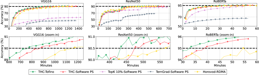
Figure 4. Time to accuracy (TTA) comparison over two image processing tasks (i.e., VGG19 and ResNet50) and an NLP task (i.e., RoBERTa). The second row zooms in on the competitive results.

Training Throughput. To examine the synchronization round time reduction we achieve with THC, we also measure the throughput in Figure 5. THC-Tofino always gives the highest throughput and achieves up to 1.58$\times$ improvement over Horovod-RDMA without compression. THC-Software PS improves the throughput by up to 1.43$\times$. THC-Tofino and THC-Software PS also give up to 1.70$\times$ and 1.61$\times$ improvement over BytePS-TCP, respectively. THC’s throughput improvement is larger for communication-intensive models (e.g., VGG16 and GPT-2).

THC-Software PS has up to 1.60$\times$ higher throughput than TopK because it eliminates the PS-side bottlenecks. While TernGrad provides high throughput, as it uses fewer bits per coordinate, and has shorter PS time and compression overhead (Section 8.2), it does not improve TTA as Fig. 4 shows.

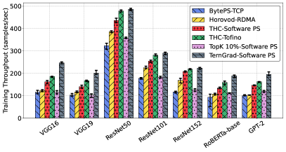
Figure 5. Training throughput with 100G links over different network- and compute-intensive architectures.

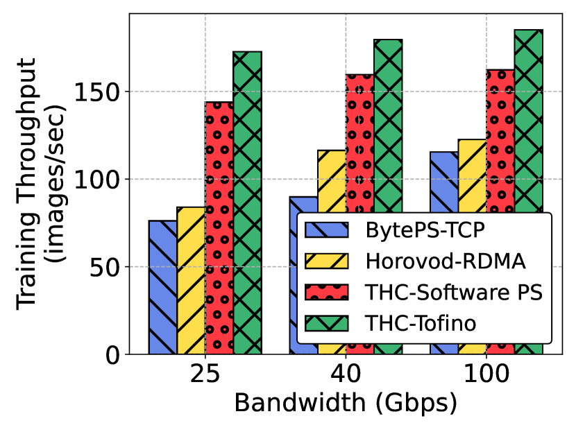
Figure 6. Training throughput for different bandwidths.

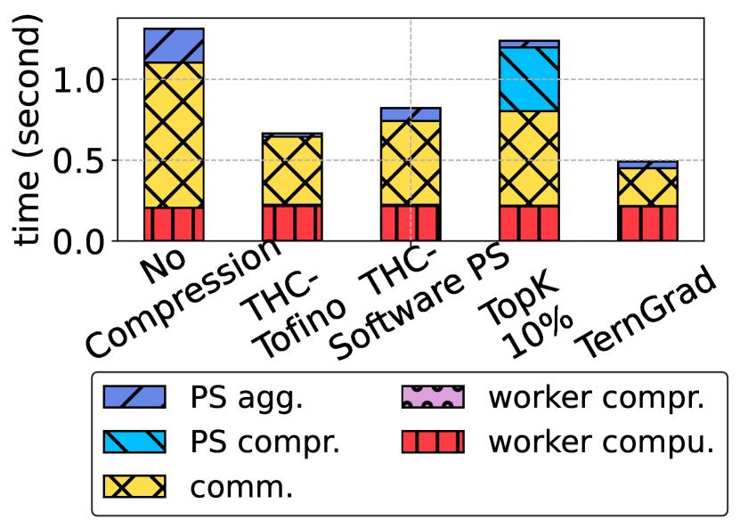
Figure 7. Average training round time breakdown.

Effectiveness with Different Bandwidth. We train the VGG16 architecture under different network bandwidth settings (25, 40, and 100Gbps) in Figure 7. THC-Tofino achieves 2.05$\times$, 1.54$\times$, and 1.51$\times$ training throughput over Horovod-RDMA at 25Gbps, 40Gbps, and 100Gbps respectively. When the bandwidth decreases from 40Gbps to 25Gbps, the throughput of Horovod-RDMA drops significantly because it faces more network bottlenecks. Meanwhile, the performance of THC-Tofino and THC-Software PS downgrades gracefully as the bandwidth decreases, leading to higher training speedups at low bandwidths. We expect THC to offer more benefits under slower networks (e.g., 10Gbps, 1Gbps) which we might encounter in federated learning settings.

8.2. Network-compute tradeoff

In Figure 7, we break down the time per iteration into the time spent at the PS, workers, and the communication, when training VGG16 at 100Gbps with THC-Tofino, THC-Software PS, TopK 10%, and TernGrad. At the PS, we measure the compression time and aggregation time. At the workers, we measure the training time and compression time.

Compared to the no-compression baseline, THC-Software PS reduces communication time by 42.4% and reduces PS time by 61.8%. As a tradeoff, we introduce compress and decompress operations on GPU on the worker side. However, these operations only increase the overall worker time by 9.5%. The result demonstrates that in distributed training settings where workers periodically synchronize a large amount of data, saving bandwidth by slightly increasing the worker GPU computation time is worthwhile. THC-Tofino achieves more savings by further reducing communication time through in-network aggregation and offloading the PS to the switches for hardware acceleration.

For TopK10%-Software PS, it has to run expensive sorting operations on the PS, introducing a significant overhead at the PS side. Therefore, although TopK10% gives similar communication time as THC-Software PS, the overall round time is 50.7% higher than that of THC-Software PS.

For TernGrad-Software PS, it uses only two bits per coordinate and only requires simple multiplications at the PS. Therefore, it has a short communication time and a short PS time. However, as we previously stressed, TernGrad produces high NMSE and might produce poor TTA results.

8.3. THC Simulation results

In order to generalize the benefit of THC to different systems, we extend the end-to-end results by simulating THC under different system configurations. The simulations first demonstrate that THC allows straightforward scaling to a larger number of workers without any decrease in accuracy. Furthermore, we find that THC has resilience to both packet loss and straggling workers under the synchronization and partial aggregation schemes that we propose.

Simulation Environment. We simulate THC on an academic cluster with 4 A100/V100 GPUs per node. Multiple worker training is mimicked by computing multiple passes of the backpropagation, storing the gradients in memory, and then aggregating the gradients before performing an update step. This allows us to compress and decompress the aggregated gradient with THC’s algorithm before the update step to reproduce the communication steps in actual systems. For the baseline, we neglect this compression/decompression step and simply aggregate the gradients.

Workloads. We train ResNet50 (He et al., 2016) models on the CIFAR100 (Krizhevsky et al., [n. d.]) dataset with a batch size 128 for all simulations. For scalability results, we use a $p$-fraction of 1/64 and the largest granularity and bit budget that a given number of workers can handle (38/16/8 granularity with 4/4/3 bit budget for 4/10/30 workers). The packet loss and straggling worker results use the following configuration: workers 10, granularity 20, $p$-fraction 1/512, and bit budget 4. Furthermore, all accuracy results are plotted using a sliding window of size 5.

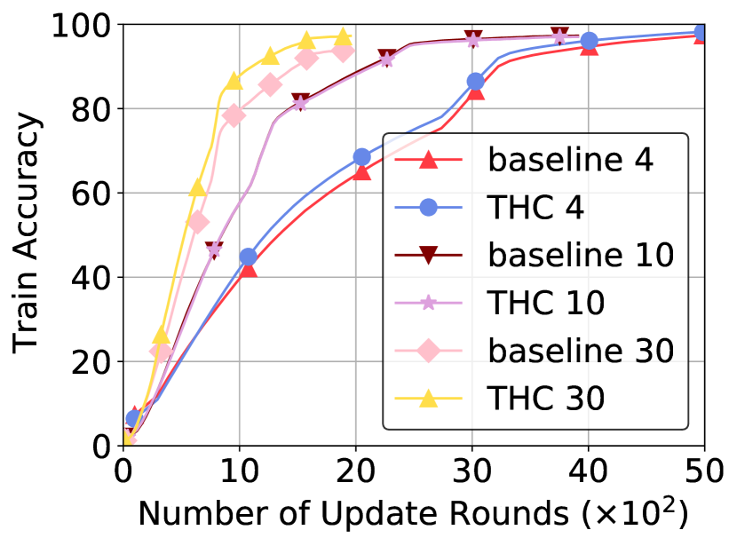
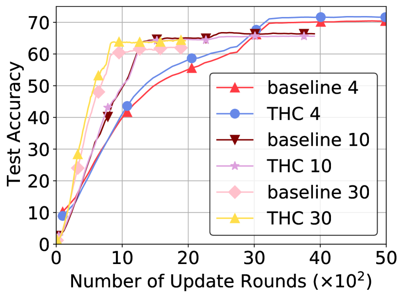
Figure 8. Scalability of THC. Displaying attainable accuracy with a different number of workers.

Scalability. To see how our system scales, we simulate THC for 4, 10, and 30 workers in Figure 8, keeping the per-worker batch size constant and tracking the accuracy against the number of model update steps. THC reaches or exceeds the baseline accuracy without compression for each configuration of workers. As a result, using 4/10/30 workers with THC reaches the target train accuracy of 95% in 3715/2503/1473 update steps, so training on THC with 30 workers is 1.7$\times$ faster than 10 workers and 2.52$\times$ faster than 4 workers assuming that the time for each update step remains constant (with similar speedups for test accuracy). Note that the higher accuracy THC achieves over the baseline for some experiments can be explained by a low learning rate causing variability in the update step: increasing the learning rate for the baseline should remove this discrepancy.

This speedup in training can be attributed to the fact that the total batch size per update step increases as we increase the number of workers without changing the per-worker batch size, allowing each update step to move further in the direction of the highest accuracy. However, the accuracy of biased compression algorithms decreases as the number of workers increases because aggregating many gradients magnifies the bias. THC on the other hand is unbiased compression, but there are three competing effects when increasing the number of workers; 1) Compressing more gradients at the same time increases the maximal norm which results in a higher error of the compression; 2) Since the compression is unbiased, increasing the number of aggregated gradients lowers the compression error; 3) We must decrease the granularity for a larger number of workers to prevent overflow, which increases the error. Points 2 and 3 can be seen from our results in Figure 10 in Appendix C. Combined, THC is still accurate enough to reach baseline accuracy with 30 workers, allowing for faster training.

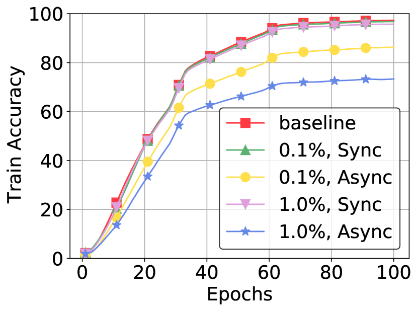
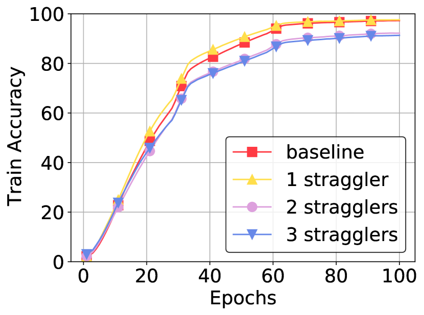
Figure 9. Resiliency to Gradient Losses. Displaying attainable accuracy with packet drops and stragglers.

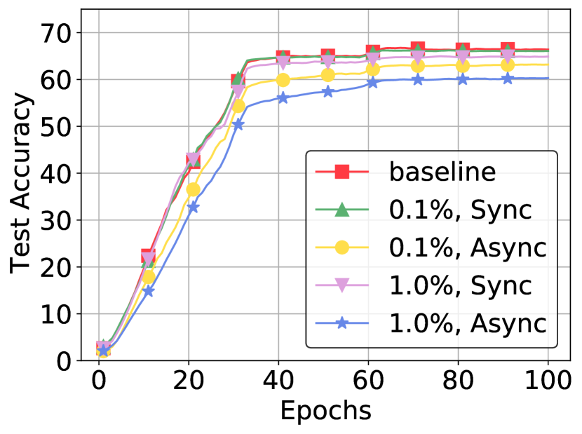
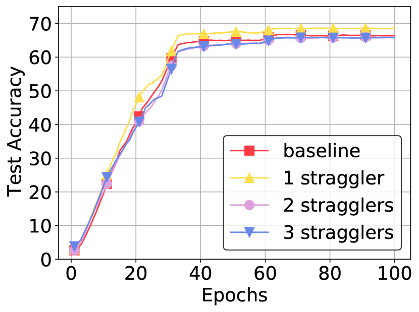
Figure 11. Test Accuracy with Gradient Losses

Packet Loss. Though we mentioned that our network has a negligible loss rate in Section 6, we show that THC can retain accuracy even in much lossier networks by artificially simulating dropped packets as 0s in the gradient. Figure 9 shows that even with a packet loss rate of 1%, which greatly decreases the final training accuracy, our proposed synchronization scheme where workers coordinate their model parameters after every epoch reduces the training accuracy drop from 24% to 1.5%. With 0.1% packet loss, synchronization reduces the accuracy discrepancy from 11% to 0.5%, which is nearly indistinguishable from baseline. The test accuracies in Figure 11 of Appendix C show similar results.

Since we simulate packet losses in both directions, these results also show that packet losses moving from the PS to the worker are more problematic, since dropped packets from the PS can result in workers having slightly different models. Over time, the error can accumulate and make the aggregated gradient nonsensical, but this is solved by our synchronization round.

Straggler Simulation. To mitigate the straggler problem, we propose and simulate a scheme where we only wait for the top n% of the workers before proceeding with the aggregation. Figure 9 shows the effect of randomly choosing a 1/2/3 stragglers during each round and dropping their gradient. With 10 workers, this corresponds to waiting for 90%/80%/70% of the workers. Waiting for the top 90% reaches the baseline accuracy, whereas 80% and 70% show only a 5-6% decrease in final training accuracy. As such, a scheme that waits for some large percentage of workers before proceeding with aggregation should be able to reliably deal with straggling workers without drops in accuracy.

9. Related Work

Systems Support for Gradient Compression. Previous gradient compression systems (e.g., HiPress (Bai et al., 2021) and Espresso (Wang et al., 2023)) focus on compression awareness and finding compression strategies and work division (e.g., compression on GPU or CPU). These systems maximize the overlap of efficient communication and compression to hide existing overhead. THC, on the other hand, mitigates compression overhead by reducing the number of compress/decompress operations. THC is complementary with these works.

In-network Aggregation for ML. SwitchML (Sapio et al., 2021) and ATP (Lao et al., 2021) have demonstrated the benefits of aggregating gradients within networks, but they do not support compression as the data is restricted to the format that can be directly aggregated. OmniReduce (Fei et al., 2021) and ASK (He et al., 2023) propose using a key-value data structure for in-network aggregation. However, these approaches require compressing the gradient data into the key-value format and make assumptions about the data itself. In THC, we support aggregation directly on compressed data, making it orthogonal to previous works. This leads to efficient in-network aggregation with compression.

10. Conclusion and Future Work

THC is a novel framework that formally defines homomorphic compression. As homomorphic compression supports direct aggregation of compressed data, it also allows an elegant combination of gradient compression and in-network aggregation. To demonstrate THC’s generalizability, we build a distributed DNN training system prototype that employs both the THC algorithm and in-network aggregation to accelerate gradient synchronization. Testbed experiments with four GPU workers, one programmable switch, and 100Gbps network show that our system prototype achieves up to 1.51$\times$ TTA improvement when we enable both gradient compression and in-network aggregation.

An important future research direction is incorporating homomorphic compression in all-reduce. Currently, compression schemes fail to improve the performance of all reduce (Agarwal et al., 2022). For example, in the widely-deployed ring all-reduce that requires $O(n^{2})$ aggregation operations, existing schemes would need an excessive number of decompression and re-compression operations, leading to poor accuracy and slowdown compared to an uncompressed baseline. THC makes the first step towards making compression algorithms all-reduce friendly. For example, we may run the reduce operation directly on gradients compressed with Uniform THC using the same number of bits required for the PS aggregation (e.g., 8). However, this method is not compatible with our various optimizations, such as sending just $b$ (e.g., 4) bits or using the lookup table, and is thus sub-optimal.

Appendix A Uniform THC Preliminaries

Given a bandwidth budget of $b$ bits per coordinate (e.g., per gradient entry), we define a compression scheme using a pair of compression and decompression operators.

Definition 0 (compression operator).

A compression operator $C:\mathbb{R}^{d}\to\{0,1\}^{b\cdot d}$ takes a real-valued $d$-dimensional vector and outputs a $(b\cdot d)$-bits compressed representation.

Definition 0 (decompression operator).

A decompression operator $D:\{0,1\}^{b\cdot d}\to\mathbb{R}^{d}$ takes a $(b\cdot d)$-bits compressed representation and outputs a real-valued $d$-dimensional estimate of the input vector.

More generally, a compression scheme may require sending some additional information. We, therefore, allow $b\cdot d+O(1)$ bits in practice.

For a vector $x\in\mathbb{R}^{d}$, we denote its estimate by $\widehat{x}=D(C(x))$. The goal of a compression scheme is then, given a bandwidth budget $b$, to minimize some error metric, e.g., the expected squared error, $\mathbb{E}[\left\lVert x-\widehat{x}\right\rVert^{2}]$. Before describing THC, for ease of presentation, we present a simplified (uniform) version of the THC framework and later generalize it.

A.1. Uniform homomorphic compression

In distributed deep learning, at each training round, the mean of the workers’ gradients forms the update of the model’s parameters for the next round. Without compression, we could add all the workers’ gradients and divide the results by the number of workers.

To reduce the bandwidth with a minimal impact on accuracy, the Distributed Mean Estimation (DME) problem has been extensively studied (Suresh et al., 2017; Safaryan et al., 2020; Lyubarskii and Vershynin, 2010; Vargaftik et al., 2021, 2022; Alistarh et al., 2017; Konečnỳ and Richtárik, 2018). Namely, in DME, workers compress their gradients before sending them for aggregation. Most DME works only consider compression in this direction, while messages from the parameter server to workers remain uncompressed. To achieve bidirectional compression, several works further suggest that the server, after decompressing and aggregating the gradients, will re-compress the result before sending it back (e.g., (Gruntkowska et al., 2022; Philippenko and Dieuleveut, 2020)), introducing additional delay and error. Avoiding these problems motivates the following definition; for convenience, we henceforth denote $\left\langle i\right\rangle=\left\{0,\ldots,i-1\right\}$ for any $i\in\mathbb{N}$.

Definition 0 (Uniform homomorphic compression).

We say that a compression scheme $(C,D)$ is uniform homomorphic if for any $n,d\in\mathbb{N}$ and $x_{0},x_{1},\ldots,x_{n-1}\in\mathbb{R}^{d}$, it satisfies

$$\frac{1}{n}\cdot\sum_{i\in\left\langle n\right\rangle}D(C(x_{i}))=D\left(\frac{1}{n}\cdot\sum_{i\in\left\langle n\right\rangle}C(x_{i})\right).$$

That is, a Uniform Homomorphic Compression (UHC) scheme allows averaging the compressed representations and applying a single decompression invocation.

That is, by using UHC, the parameter server can sum up the compressed gradients and send $\sum_{i}C(x_{i})$ back (in compressed form) without increasing the delay and error.

A.2. Uniform stochastic quantization

Two desired properties of gradient quantization schemes in a distributed setting are unbiasedness (i.e., $\mathbb{E}[\widehat{x}]=x$) and independence (i.e., each worker makes the random choice of their quantization values independently). These features are especially useful in distributed deep learning as the errors of the different workers then cancel out on average rather than add up, leading to a better estimation of the mean.

One of the most fundamental compression techniques that offer both properties is uniform stochastic quantization (USQ). Intuitively, given a vector, $x\in\mathbb{R}^{d}$, and denoting its minimum by $m$ and maximum by $M$, using USQ to quantize each coordinate $x[j]$ to a single bit means rounding it to $m$ with probability $(x[j]-m)/(M-m)$ and to $M$ with probability $(M-x[j])/(M-m)$. That is, the sender encodes the coordinate $x[j]$ using one bit $C(x)[j]\in\left\{0,1\right\}$ and the receiver estimates it as $\widehat{x}=D(C(x))=m+(M-m)\cdot C(x)$. Note that $m$ and $M$ need to be sent to the receiver as well. However, considering that $d$ is large, this overhead is negligible.

This idea generalizes to any number of bits per coordinate $b$ by partitioning the range $[m,M]$ into $2^{b}-1$ uniform (i.e., equal-length) intervals where each entry is rounded to one of its nearest endpoints $c_{0},c_{1}$ with probabilities $(x[j]-c_{0})/(c_{1}-c_{0})$ and $(c_{1}-x[j])/(c_{1}-c_{0})$ to make the estimate unbiased. That is, when the message for coordinate $x[j]$, $C(x)[j]\in\left\langle 2^{b}\right\rangle$, is sent to the receiver that estimates the coordinate as $m+C(x)[j]\cdot(M-m)/(2^{b}-1)$.

Despite its popularity and simplicity, in our context, USQ has two main drawbacks. First, USQ is not homomorphic; this is because each worker has its own minimum and maximum values, and accordingly, the $b$-bit messages describing the same coordinate by different workers are not amenable to aggregation without decompressing the messages. Second, USQ’s error highly depends on the input vector’s distribution, e.g., the difference between the minimum and maximum. For example, for $b=1$, if the input vector is $(1,-1,0,0,\ldots,0)$, all the zero-valued coordinates will be rounded with an error of $1$, and the vector’s estimate will greatly differ from the input.

Several recent works propose pre-processing each gradient and post-processing the average’s estimate. The idea behind this approach is to change the vector’s distribution prior to quantization to avoid bad cases. For example, (Suresh et al., 2017) proposes to preprocess by applying the randomized Hadamard transform to ensure that the range is small with high probability and postprocess using the inverse transform. As another example, Kashin’s representation (Safaryan et al., 2020; Lyubarskii and Vershynin, 2010) allows projecting the vector into a higher-dimensional space with similar magnitude coefficients.

Appendix B Optimally Solving the Lookup Table Optimization Problem

As described in Section 5.3, the solution of the following optimization problem yields the optimal lookup table $T_{b,g,p}=T$. Observe that the problem depends on the parameters $b,g,p$, where $b$ is the number of bits workers send for each quantized coordinate, $g$ is the granularity (the range of values that the table can take), and $p$ is the expected fraction of transformed and scaled coordinates that are not taken into account when determining the truncation range $[-t_{p},t_{p}]$.

$\begin{array}[]{l}\displaystyle{\operatorname*{minimize}_{P,T}}\displaystyle\int_{-t_{p}}^{t_{p}}\sum_{z\in\left\langle 2^{b}\right\rangle}P(a,z)\cdot\left(a-T(z)\right)^{2}\cdot\phi(a)\cdot da\\ \vskip 6.0pt plus 2.0pt minus 2.0pt\text{subject to}\\ \vskip 6.0pt plus 2.0pt minus 2.0pt{\small(\textit{{\color[rgb]{.5,.5,.5}Unbiasedness}})}\displaystyle\ \ \sum_{z\in\left\langle 2^{b}\right\rangle}P(a,z)\cdot T(z)=a\quad\hfill\forall\,a\in[-t_{p},t_{p}]\\ \vskip 6.0pt plus 2.0pt minus 2.0pt{\small(\textit{{\color[rgb]{.5,.5,.5}Probability}})}\,\ \quad\displaystyle\sum_{z\in\left\langle 2^{b}\right\rangle}P(a,z)=1\hfill\forall\,a\in[-t_{p},t_{p}]\\ \vskip 6.0pt plus 2.0pt minus 2.0pt\quad\quad\quad\quad\quad\quad\,\,\,P(a,z)\geq 0\hfill\forall\,a\in[-t_{p},t_{p}],\,z\in\left\langle 2^{b}\right\rangle\\ \vskip 6.0pt plus 2.0pt minus 2.0pt{\small(\textit{{\color[rgb]{.5,.5,.5}Granularity}})}\quad\,\,\,T(z)\in\left\{\frac{2t_{p}}{g}\cdot i-t_{p}\mid i\in\left\langle g+1\right\rangle\right\}\hfill\quad\forall\,z\in\left\langle 2^{b}\right\rangle\end{array}$

Recall that, without loss of generality, we may assume that $0=T(0)<T(1)<\ldots<T(2^{b}-1)=g$, which significantly narrows down the search range from $\left(g+1\right)^{2^{b}}$ (which is the number of options to choose a table value for each table index). Namely, this observation means that the number of possible options for $T$ is $SaB(g-2^{b}-1,2^{b}-1)$ ($SaB$ stands for the stars-and-bars), where $SaB(n,k)={n+k-1\choose k-1}$ is the number of options for throwing $n$ identical balls into $k$ distinct bins. This is because we can think of $2^{b}-1$ bins representing the values $\left\{T(i+1)-T(i)\mid i\in\left\langle 2^{b}-1\right\rangle\right\}$; this way, ‘throwing a ball’ into the $i$’th bin corresponds to increasing the difference by $1$, and we have $g-2^{b}-1$ balls as all bins must be non-empty to enforce the strict monotonicity. The number of options is therefore $SaB(g-2^{b}-1,2^{b}-1)={g-3\choose 2^{b}-2}\ll(g+1)^{2^{b}}$. For example, if $b=4,g=51$, we reduce the number of options from $52^{15}\approx 5.5\cdot 10^{25}$ to ${48\choose 14}\approx 4.8\cdot 10^{11}$. We note that these $b,g$ values are the largest ones that we have found to be of interest as they yield a solution whose accuracy is on par with an uncompressed baseline.

To further reduce the number of options, if $g$ is odd, we leverage the symmetry of the normal distribution (i.e., that $\phi(a)=\phi(-a)$ for any $a\in\mathbb{R}$). In particular, together with the fact that the number of table indices is even, this implies that a table index $T(z)$ exists in the optimal table if and only if there exists $z^{\prime}$ such that $T(z^{\prime})=g-T(z)$. In particular, this can be manifested as the following additional constraint:

$\begin{array}[]{l}{\small(\textit{{\color[rgb]{.5,.5,.5}symmetry}})}\quad\,\,\,T(z)=T(z+2^{b-1})-\frac{g+1}{2}\hfill\quad\forall\,z\in\left\langle 2^{b-1}\right\rangle\end{array}$

Notice that this further reduces the number of options to $SaB\left(\frac{g+1}{2}-2^{b-1}-1,2^{b-1}-1\right)$. Using the $b=4,g=51$ example, we reduced the number of options to just $100947$.

This allows us to efficiently solve the problem optimally by computing the target integral for every possible value of $T$. For each value, we use the fact that stochastic quantization (picking one of the two closest quantization values with probabilities that make it unbiased) is optimal given the quantization values (Basat et al., 2021). In particular, this means that we can easily derive the optimal $P$ values and thus compute the integral. For example, if $b=2,g=4$ and $T(0)=0,T(1)=1,T(2)=3,T(3)=4$, we can compute the integral as:

$\begin{array}[]{l}\displaystyle\int_{-t_{p}}^{-t_{p}/2}\left(\frac{a-(-t_{p})}{t_{p}/2}\cdot\left(a-(-t_{p}/2)\right)^{2}+\frac{-t_{p}/2-a}{t_{p}/2}\cdot\left(a-(-t_{p})\right)^{2}\right)\cdot\phi(a)\cdot da\\ \\ +\displaystyle\int_{-t_{p}/2}^{t_{p}/2}\left(\frac{a-(-t_{p}/2)}{t_{p}}\cdot\left(a-t_{p}/2\right)^{2}+\frac{t_{p}/2-a}{t_{p}}\cdot\left(a-(-t_{p}/2)\right)^{2}\right)\cdot\phi(a)\cdot da\\ \\ +\displaystyle\int_{t_{p}/2}^{t_{p}}\left(\frac{a-t_{p}/2}{t_{p}/2}\cdot\left(a-t_{p}\right)^{2}+\frac{t_{p}-a}{t_{p}/2}\cdot\left(a-t_{p}/2\right)^{2}\right)\cdot\phi(a)\cdot da\end{array}$

Enumerating over the options: The last ingredient in our solver is a simple method to iterate over all the stars-and-bars options. Namely, consider wanting to throw $n$ balls into $k$ bins and let $B[i]$ denote the number of balls in the $i$’th bin. Then, the enumeration process is given by Algorithm 5.

Algorithm 5 Stars-and-Bars $(n,k)$ Enumeration

1:Initialize $B[0]=n,\quad B[1]=B[2]=\ldots,B[k-1]=0$

2:Yield$(B)$ $\triangleright$  This is the $0$’th option

3:for $j=1,2,\ldots,SaB(n,k)-1$ do

4:    $a=\min\left\{i\mid B[i]>0\right\}$

5:    $B[a+1]=B[a+1]+1$

6:    $S=B[a]-1$

7:    $B[a]=0$

8:    $B[0]=S$

9:    Yield$(B)$ $\triangleright$  $B$ is the $j$’th option

10:end for

The resulting solver is quite efficient: we ran it once for each of over $4000$ different $(b,g,p)$ combinations and computed all the optimal tables within mere minutes.

Appendix C EVALUATION FIGURES

C.1. NMSE for Different THC Parameters

We repeatedly compute the NMSE of the compression under different parameters of THC. A gradient is first drawn from a log-normal distribution and then copied multiple times to match the number of simulated workers. We run THC on the copies of the gradient and compute the NMSE. Repeating 100 times, we report the average NMSE as we scale the number of workers and increase the granularity. For the granularity experiments, we simulated 10 workers and used a $p$-fraction of 1/1024. The experiments with the number of workers were completed with a granularity of 36/36/38 for 2/3/4 bit budget and a $p$-fraction of 1/32.

In Figure 10, we first note that the largest discrepancy in NMSE is between different bit budgets where the error decreases by almost an order of magnitude between bit budgets of 2 to 3 to 4. The bit budget corresponds directly to the compression ratio of the algorithm, so it is expected that the accuracy should increase as we use more bits for compression. Furthermore, the NMSE of THC also decreases as the granularity increases since larger granularity values allows for more fine-grained choices of quantization values, though this effect is more difficult to see. Lastly, the error decreases as the number of simulated workers increases as we expect given that the decompressed gradient acts as an unbiased estimator of the aggregated gradient.

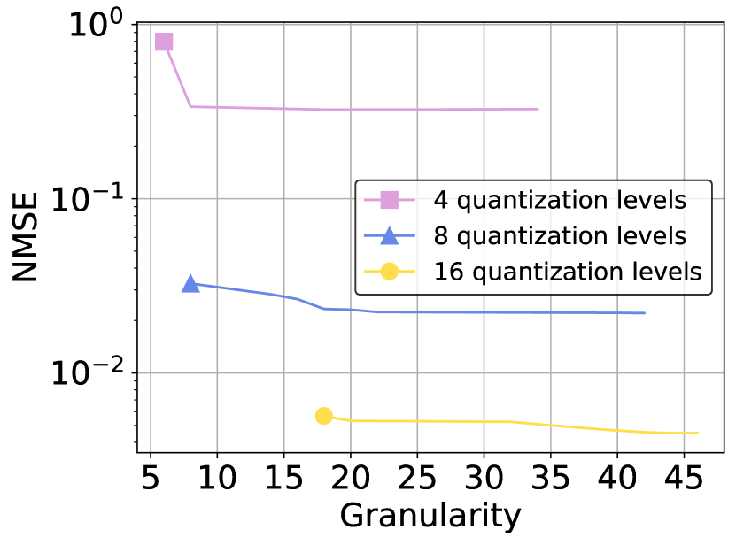
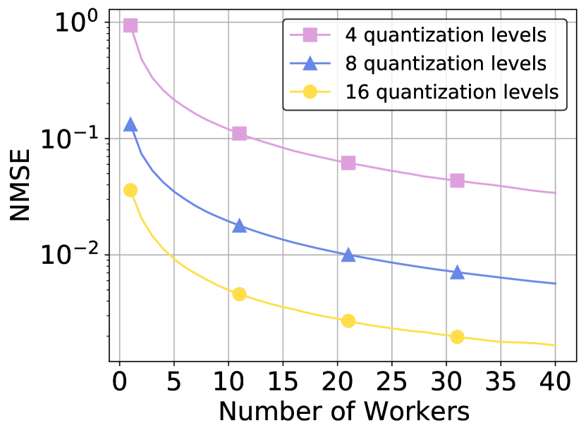
Figure 10. NMSE under different granularities and number of workers (plotted on log scale)

C.2. Test Accuracies for Resiliency Results

Similar to the training accuracy results, the test accuracy shows that synchronization is very beneficial when the system is lossy and that waiting for the top 90% of workers does not affect the final accuracy. Under 1%/0.1% loss, the discrepancy from baseline drops from 6%/3.2% to 1.5%/0.4%. For 80%/70% stragglers, the error from baseline is roughly 0.5%.

References

- (1)
- roc (2014) 2014. InfiniBand Trade Association. RoCE v2 Specification. . https://cw.infinibandta.org/document/dl/7781. (2014).
- NVI (2020) 2020. NVIDIA Scalable Hierarchical Aggregation and Reduction Protocol (SHARP). . https://docs.nvidia.com/networking/display/SHARPv200. (2020).
- vit (2023) 2023. Vitis AI. https://www.xilinx.com/products/design-tools/vitis/vitis-ai.html. (2023).
- Agarwal et al. (2022) Saurabh Agarwal, Hongyi Wang, Shivaram Venkataraman, and Dimitris Papailiopoulos. 2022. On the Utility of Gradient Compression in Distributed Training Systems. In Proceedings of Machine Learning and Systems, D. Marculescu, Y. Chi, and C. Wu (Eds.), Vol. 4. 652–672. https://proceedings.mlsys.org/paper/2022/file/cedebb6e872f539bef8c3f919874e9d7-Paper.pdf
- Ailon and Chazelle (2006) Nir Ailon and Bernard Chazelle. 2006. Approximate nearest neighbors and the fast Johnson-Lindenstrauss transform. In Proceedings of the thirty-eighth annual ACM symposium on Theory of computing. 557–563.
- Alistarh et al. (2017) Dan Alistarh, Demjan Grubic, Jerry Z. Li, Ryota Tomioka, and Milan Vojnovic. 2017. QSGD: Communication-Efficient SGD via Gradient Quantization and Encoding. In Proceedings of the 31st International Conference on Neural Information Processing Systems (NIPS’17). Curran Associates Inc., Red Hook, NY, USA, 1707–1718.
- Bai et al. (2021) Youhui Bai, Cheng Li, Quan Zhou, Jun Yi, Ping Gong, Feng Yan, Ruichuan Chen, and Yinlong Xu. 2021. Gradient Compression Supercharged High-Performance Data Parallel DNN Training. In Proceedings of the ACM SIGOPS 28th Symposium on Operating Systems Principles (SOSP ’21). Association for Computing Machinery, New York, NY, USA, 359–375. https://doi.org/10.1145/3477132.3483553
- Basat et al. (2021) Ran Ben Basat, Michael Mitzenmacher, and Shay Vargaftik. 2021. How to Send a Real Number Using a Single Bit (And Some Shared Randomness). In 48th International Colloquium on Automata, Languages, and Programming, ICALP 2021, July 12-16, 2021, Glasgow, Scotland (Virtual Conference) (LIPIcs), Nikhil Bansal, Emanuela Merelli, and James Worrell (Eds.), Vol. 198. Schloss Dagstuhl - Leibniz-Zentrum für Informatik, 25:1–25:20. https://doi.org/10.4230/LIPIcs.ICALP.2021.25
- Bernstein et al. (2018) Jeremy Bernstein, Yu-Xiang Wang, Kamyar Azizzadenesheli, and Animashree Anandkumar. 2018. signSGD: Compressed optimisation for non-convex problems. In International Conference on Machine Learning. PMLR, 560–569.
- Brown et al. (2020) Tom Brown, Benjamin Mann, Nick Ryder, Melanie Subbiah, Jared D Kaplan, Prafulla Dhariwal, Arvind Neelakantan, Pranav Shyam, Girish Sastry, Amanda Askell, et al. 2020. Language models are few-shot learners. Advances in neural information processing systems 33 (2020), 1877–1901.
- Cohen et al. (2022) Aaron Daniel Cohen, Adam Roberts, Alejandra Molina, Alena Butryna, Alicia Jin, Apoorv Kulshreshtha, Ben Hutchinson, Ben Zevenbergen, Blaise Hilary Aguera-Arcas, Chung ching Chang, Claire Cui, Cosmo Du, Daniel De Freitas Adiwardana, Dehao Chen, Dmitry (Dima) Lepikhin, Ed H. Chi, Erin Hoffman-John, Heng-Tze Cheng, Hongrae Lee, Igor Krivokon, James Qin, Jamie Hall, Joe Fenton, Johnny Soraker, Kathy Meier-Hellstern, Kristen Olson, Lora Mois Aroyo, Maarten Paul Bosma, Marc Joseph Pickett, Marcelo Amorim Menegali, Marian Croak, Mark Díaz, Matthew Lamm, Maxim Krikun, Meredith Ringel Morris, Noam Shazeer, Quoc V. Le, Rachel Bernstein, Ravi Rajakumar, Ray Kurzweil, Romal Thoppilan, Steven Zheng, Taylor Bos, Toju Duke, Tulsee Doshi, Vincent Y. Zhao, Vinodkumar Prabhakaran, Will Rusch, YaGuang Li, Yanping Huang, Yanqi Zhou, Yuanzhong Xu, and Zhifeng Chen. 2022. LaMDA: Language Models for Dialog Applications. In arXiv.
- Devlin et al. (2018) Jacob Devlin, Ming-Wei Chang, Kenton Lee, and Kristina Toutanova. 2018. Bert: Pre-training of deep bidirectional transformers for language understanding. arXiv preprint arXiv:1810.04805 (2018).
- Fei et al. (2021) Jiawei Fei, Chen-Yu Ho, Atal N. Sahu, Marco Canini, and Amedeo Sapio. 2021. Efficient Sparse Collective Communication and Its Application to Accelerate Distributed Deep Learning. In Proceedings of the 2021 ACM SIGCOMM 2021 Conference (SIGCOMM ’21). Association for Computing Machinery, New York, NY, USA, 676–691. https://doi.org/10.1145/3452296.3472904
- Fowers et al. (2018) Jeremy Fowers, Kalin Ovtcharov, Michael Papamichael, Todd Massengill, Ming Liu, Daniel Lo, Shlomi Alkalay, Michael Haselman, Logan Adams, Mahdi Ghandi, Stephen Heil, Prerak Patel, Adam Sapek, Gabriel Weisz, Lisa Woods, Sitaram Lanka, Steven K. Reinhardt, Adrian M. Caulfield, Eric S. Chung, and Doug Burger. 2018. A Configurable Cloud-Scale DNN Processor for Real-Time AI. In 2018 ACM/IEEE 45th Annual International Symposium on Computer Architecture (ISCA). 1–14. https://doi.org/10.1109/ISCA.2018.00012
- Gebara et al. (2021) Nadeen Gebara, Manya Ghobadi, and Paolo Costa. 2021. In-network Aggregation for Shared Machine Learning Clusters. In Proceedings of Machine Learning and Systems, A. Smola, A. Dimakis, and I. Stoica (Eds.), Vol. 3. 829–844. https://proceedings.mlsys.org/paper/2021/file/eae27d77ca20db309e056e3d2dcd7d69-Paper.pdf
- Gruntkowska et al. (2022) Kaja Gruntkowska, Alexander Tyurin, and Peter Richtárik. 2022. EF21-P and Friends: Improved Theoretical Communication Complexity for Distributed Optimization with Bidirectional Compression. arXiv preprint arXiv:2209.15218 (2022).
- He et al. (2016) K. He, X. Zhang, S. Ren, and J. Sun. 2016. Deep Residual Learning for Image Recognition. In 2016 IEEE Conference on Computer Vision and Pattern Recognition (CVPR). 770–778. https://doi.org/10.1109/CVPR.2016.90
- He et al. (2023) Yongchao He, Wenfei Wu, Yanfang Le, Ming Liu, and ChonLam Lao. 2023. A Generic Service to Provide In-Network Aggregation for Key-Value Streams. In Proceedings of the 28th ACM International Conference on Architectural Support for Programming Languages and Operating Systems, Volume 2 (ASPLOS 2023). Association for Computing Machinery, New York, NY, USA, 33–47. https://doi.org/10.1145/3575693.3575708
- Hedayat and Wallis (1978) A Hedayat and Walter Dennis Wallis. 1978. Hadamard matrices and their applications. The Annals of Statistics (1978), 1184–1238.
- Jeon et al. (2019) Myeongjae Jeon, Shivaram Venkataraman, Amar Phanishayee, Junjie Qian, Wencong Xiao, and Fan Yang. 2019. Analysis of Large-Scale Multi-Tenant GPU Clusters for DNN Training Workloads. In 2019 USENIX Annual Technical Conference (USENIX ATC 19). USENIX Association, Renton, WA, 947–960. https://www.usenix.org/conference/atc19/presentation/jeon
- Jiang et al. (2020) Yimin Jiang, Yibo Zhu, Chang Lan, Bairen Yi, Yong Cui, and Chuanxiong Guo. 2020. A Unified Architecture for Accelerating Distributed DNN Training in Heterogeneous GPU/CPU Clusters. In 14th USENIX Symposium on Operating Systems Design and Implementation (OSDI 20). USENIX Association, 463–479. https://www.usenix.org/conference/osdi20/presentation/jiang
- Jouppi et al. (2017) Norman P. Jouppi, Cliff Young, Nishant Patil, David Patterson, Gaurav Agrawal, Raminder Bajwa, Sarah Bates, Suresh Bhatia, Nan Boden, Al Borchers, Rick Boyle, Pierre luc Cantin, Clifford Chao, Chris Clark, Jeremy Coriell, Mike Daley, Matt Dau, Jeffrey Dean, Ben Gelb, Tara Vazir Ghaemmaghami, Rajendra Gottipati, William Gulland, Robert Hagmann, C. Richard Ho, Doug Hogberg, John Hu, Robert Hundt, Dan Hurt, Julian Ibarz, Aaron Jaffey, Alek Jaworski, Alexander Kaplan, Harshit Khaitan, Andy Koch, Naveen Kumar, Steve Lacy, James Laudon, James Law, Diemthu Le, Chris Leary, Zhuyuan Liu, Kyle Lucke, Alan Lundin, Gordon MacKean, Adriana Maggiore, Maire Mahony, Kieran Miller, Rahul Nagarajan, Ravi Narayanaswami, Ray Ni, Kathy Nix, Thomas Norrie, Mark Omernick, Narayana Penukonda, Andy Phelps, and Jonathan Ross. 2017. In-Datacenter Performance Analysis of a Tensor Processing Unit. https://arxiv.org/pdf/1704.04760.pdf
- Karimireddy et al. (2019) Sai Praneeth Karimireddy, Quentin Rebjock, Sebastian Stich, and Martin Jaggi. 2019. Error feedback fixes signsgd and other gradient compression schemes. In International Conference on Machine Learning. PMLR, 3252–3261.
- Keskar et al. (2017) Nitish Shirish Keskar, Dheevatsa Mudigere, Jorge Nocedal, Mikhail Smelyanskiy, and Ping Tak Peter Tang. 2017. On Large-Batch Training for Deep Learning: Generalization Gap and Sharp Minima. In International Conference on Learning Representations.
- Konečnỳ and Richtárik (2018) Jakub Konečnỳ and Peter Richtárik. 2018. Randomized distributed mean estimation: Accuracy vs. communication. Frontiers in Applied Mathematics and Statistics 4 (2018), 62.
- Krizhevsky et al. ([n. d.]) Alex Krizhevsky, Vinod Nair, and Geoffrey Hinton. [n. d.]. CIFAR-100 (Canadian Institute for Advanced Research). ([n. d.]). http://www.cs.toronto.edu/~kriz/cifar.html
- Lao et al. (2021) ChonLam Lao, Yanfang Le, Kshiteej Mahajan, Yixi Chen, Wenfei Wu, Aditya Akella, and Michael Swift. 2021. ATP: In-network Aggregation for Multi-tenant Learning. In 18th USENIX Symposium on Networked Systems Design and Implementation (NSDI 21). USENIX Association, 741–761. https://www.usenix.org/conference/nsdi21/presentation/lao
- Li et al. (2014) Mu Li, David G. Andersen, Jun Woo Park, Alexander J. Smola, Amr Ahmed, Vanja Josifovski, James Long, Eugene J. Shekita, and Bor-Yiing Su. 2014. Scaling Distributed Machine Learning with the Parameter Server. In Operating Systems Design and Implementation. USENIX, 583–598.
- Liu et al. (2019) Yinhan Liu, Myle Ott, Naman Goyal, Jingfei Du, Mandar Joshi, Danqi Chen, Omer Levy, Mike Lewis, Luke Zettlemoyer, and Veselin Stoyanov. 2019. RoBERTa: A Robustly Optimized BERT Pretraining Approach. CoRR abs/1907.11692 (2019). arXiv:1907.11692 http://arxiv.org/abs/1907.11692
- Lyubarskii and Vershynin (2010) Yurii Lyubarskii and Roman Vershynin. 2010. Uncertainty Principles and Vector Quantization. IEEE Transactions on Information Theory 56, 7 (2010), 3491–3501.
- McDanel et al. (2019) Bradley McDanel, Sai Qian Zhang, H. T. Kung, and Xin Dong. 2019. Full-Stack Optimization for Accelerating CNNs Using Powers-of-Two Weights with FPGA Validation. In Proceedings of the ACM International Conference on Supercomputing (ICS ’19). Association for Computing Machinery, New York, NY, USA, 449–460. https://doi.org/10.1145/3330345.3330385
- Narayanan et al. (2021) Deepak Narayanan, Mohammad Shoeybi, Jared Casper, Patrick LeGresley, Mostofa Patwary, Vijay Korthikanti, Dmitri Vainbrand, Prethvi Kashinkunti, Julie Bernauer, Bryan Catanzaro, Amar Phanishayee, and Matei Zaharia. 2021. Efficient Large-Scale Language Model Training on GPU Clusters Using Megatron-LM. In Proceedings of the International Conference for High Performance Computing, Networking, Storage and Analysis (SC ’21). Association for Computing Machinery, New York, NY, USA, Article 58, 15 pages. https://doi.org/10.1145/3458817.3476209
- Naumov et al. (2019) Maxim Naumov, Dheevatsa Mudigere, Hao-Jun Michael Shi, Jianyu Huang, Narayanan Sundaraman, Jongsoo Park, Xiaodong Wang, Udit Gupta, Carole-Jean Wu, Alisson G Azzolini, et al. 2019. Deep learning recommendation model for personalization and recommendation systems. arXiv preprint arXiv:1906.00091 (2019).
- Patarasuk and Yuan (2009) Pitch Patarasuk and Xin Yuan. 2009. Bandwidth Optimal Allreduce Algorithms for Clusters of Workstations. J. Parallel and Distrib. Comput. 69, 2 (2009), 117–124.
- Peng et al. (2019) Yanghua Peng, Yibo Zhu, Yangrui Chen, Yixin Bao, Bairen Yi, Chang Lan, Chuan Wu, and Chuanxiong Guo. 2019. A Generic Communication Scheduler for Distributed DNN Training Acceleration. In Proceedings of the 27th ACM Symposium on Operating Systems Principles (SOSP ’19). Association for Computing Machinery, New York, NY, USA, 16–29. https://doi.org/10.1145/3341301.3359642
- Petrica et al. (2020) Lucian Petrica, Tobias Alonso, Mairin Kroes, Nicholas Fraser, Sorin Cotofana, and Michaela Blott. 2020. Memory-Efficient Dataflow Inference for Deep CNNs on FPGA. In 2020 International Conference on Field-Programmable Technology (ICFPT). 48–55. https://doi.org/10.1109/ICFPT51103.2020.00016
- Philippenko and Dieuleveut (2020) Constantin Philippenko and Aymeric Dieuleveut. 2020. Bidirectional compression in heterogeneous settings for distributed or federated learning with partial participation: tight convergence guarantees. arXiv preprint arXiv:2006.14591 (2020).
- Ports and Nelson (2019) Dan R. K. Ports and Jacob Nelson. 2019. When Should The Network Be The Computer?. In Proceedings of the Workshop on Hot Topics in Operating Systems (HotOS ’19). Association for Computing Machinery, New York, NY, USA, 209–215. https://doi.org/10.1145/3317550.3321439
- Radford et al. (2019) Alec Radford, Jeffrey Wu, Rewon Child, David Luan, Dario Amodei, Ilya Sutskever, et al. 2019. Language models are unsupervised multitask learners. OpenAI blog 1, 8 (2019), 9.
- Rajbhandari et al. (2022) Samyam Rajbhandari, Conglong Li, Zhewei Yao, Minjia Zhang, Reza Yazdani Aminabadi, Ammar Ahmad Awan, Jeff Rasley, and Yuxiong He. 2022. DeepSpeed-MoE: Advancing Mixture-of-Experts Inference and Training to Power Next-Generation AI Scale. In Proceedings of the 39th International Conference on Machine Learning (Proceedings of Machine Learning Research), Kamalika Chaudhuri, Stefanie Jegelka, Le Song, Csaba Szepesvari, Gang Niu, and Sivan Sabato (Eds.), Vol. 162. PMLR, 18332–18346. https://proceedings.mlr.press/v162/rajbhandari22a.html
- Ramezani-Kebrya et al. (2021) Ali Ramezani-Kebrya, Fartash Faghri, Ilya Markov, Vitalii Aksenov, Dan Alistarh, and Daniel M Roy. 2021. NUQSGD: Provably Communication-efficient Data-parallel SGD via Nonuniform Quantization. J. Mach. Learn. Res. 22 (2021), 114–1.
- Redmon et al. (2016) Joseph Redmon, Santosh Divvala, Ross Girshick, and Ali Farhadi. 2016. You Only Look Once: Unified, Real-Time Object Detection. In Proceedings of the IEEE Conference on Computer Vision and Pattern Recognition (CVPR).
- Russakovsky et al. (2015) Olga Russakovsky, Jia Deng, Hao Su, Jonathan Krause, Sanjeev Satheesh, Sean Ma, Zhiheng Huang, Andrej Karpathy, Aditya Khosla, Michael Bernstein, Alexander C. Berg, and Li Fei-Fei. 2015. ImageNet Large Scale Visual Recognition Challenge. International Journal of Computer Vision (IJCV) 115, 3 (2015), 211–252. https://doi.org/10.1007/s11263-015-0816-y
- Safaryan et al. (2020) Mher Safaryan, Egor Shulgin, and Peter Richtárik. 2020. Uncertainty Principle for Communication Compression in Distributed and Federated Learning and the Search for an Optimal Compressor. arXiv preprint arXiv:2002.08958 (2020).
- Sapio et al. (2021) Amedeo Sapio, Marco Canini, Chen-Yu Ho, Jacob Nelson, Panos Kalnis, Changhoon Kim, Arvind Krishnamurthy, Masoud Moshref, Dan Ports, and Peter Richtarik. 2021. Scaling Distributed Machine Learning with In-Network Aggregation. In 18th USENIX Symposium on Networked Systems Design and Implementation (NSDI 21). USENIX Association, 785–808. https://www.usenix.org/conference/nsdi21/presentation/sapio
- Sergeev and Del Balso (2018) Alexander Sergeev and Mike Del Balso. 2018. Horovod: fast and easy distributed deep learning in TensorFlow. arXiv preprint arXiv:1802.05799 (2018).
- Sevilla et al. (2022) Jaime Sevilla, Lennart Heim, Anson Ho, Tamay Besiroglu, Marius Hobbhahn, and Pablo Villalobos. 2022. Compute Trends Across Three Eras of Machine Learning. arXiv preprint arXiv:2202.05924 (2022).
- Shazeer et al. (2017) Noam Shazeer, Azalia Mirhoseini, Krzysztof Maziarz, Andy Davis, Quoc Le, Geoffrey Hinton, and Jeff Dean. 2017. Outrageously large neural networks: The sparsely-gated mixture-of-experts layer. arXiv preprint arXiv:1701.06538 (2017).
- Simonyan and Zisserman (2014) Karen Simonyan and Andrew Zisserman. 2014. Very Deep Convolutional Networks for Large-Scale Image Recognition. (2014). https://doi.org/10.48550/ARXIV.1409.1556
- Socher et al. (2013) Richard Socher, Alex Perelygin, Jean Wu, Jason Chuang, Christopher D Manning, Andrew Y Ng, and Christopher Potts. 2013. Recursive deep models for semantic compositionality over a sentiment treebank. In Proceedings of the 2013 conference on empirical methods in natural language processing. 1631–1642.
- Stich et al. (2018) Sebastian U. Stich, Jean-Baptiste Cordonnier, and Martin Jaggi. 2018. Sparsified SGD with Memory. In Proceedings of the 32nd International Conference on Neural Information Processing Systems (NIPS’18). Curran Associates Inc., Red Hook, NY, USA, 4452–4463.
- Sun et al. (2019) Peng Sun, Wansen Feng, Ruobing Han, Shengen Yan, and Yonggang Wen. 2019. Optimizing Network Performance for Distributed DNN Training on GPU Clusters: ImageNet/AlexNet Training in 1.5 Minutes. (2019). https://doi.org/10.48550/ARXIV.1902.06855
- Suresh et al. (2017) Ananda Theertha Suresh, X Yu Felix, Sanjiv Kumar, and H Brendan McMahan. 2017. Distributed Mean Estimation With Limited Communication. In International Conference on Machine Learning. PMLR, 3329–3337.
- Vargaftik et al. (2022) Shay Vargaftik, Ran Ben Basat, Amit Portnoy, Gal Mendelson, Yaniv Ben Itzhak, and Michael Mitzenmacher. 2022. Eden: Communication-efficient and robust distributed mean estimation for federated learning. In International Conference on Machine Learning. PMLR, 21984–22014.
- Vargaftik et al. (2021) Shay Vargaftik, Ran Ben-Basat, Amit Portnoy, Gal Mendelson, Yaniv Ben-Itzhak, and Michael Mitzenmacher. 2021. Drive: One-bit distributed mean estimation. Advances in Neural Information Processing Systems 34 (2021), 362–377.
- Wang et al. (2016) Wei Wang, Meihui Zhang, Gang Chen, H. V. Jagadish, Beng Chin Ooi, and Kian-Lee Tan. 2016. Database Meets Deep Learning: Challenges and Opportunities. SIGMOD Rec. 45, 2 (Sept. 2016), 17–22. https://doi.org/10.1145/3003665.3003669
- Wang et al. (2023) Zhuang Wang, Haibin Lin, Yibo Zhu, and TS Eugene Ng. 2023. Hi-Speed DNN Training with Espresso: Unleashing the Full Potential of Gradient Compression with Near-Optimal Usage Strategies. In Proceedings of the Eighteenth European Conference on Computer Systems. ssociation for Computing Machinery, TBA.
- Wang and O’Boyle (2018) Zheng Wang and Michael O’Boyle. 2018. Machine learning in compiler optimization. Proc. IEEE 106, 11 (2018), 1879–1901.
- Wen et al. (2017) Wei Wen, Cong Xu, Feng Yan, Chunpeng Wu, Yandan Wang, Yiran Chen, and Hai Li. 2017. TernGrad: Ternary Gradients to Reduce Communication in Distributed Deep Learning. In Proceedings of the 31st International Conference on Neural Information Processing Systems (NIPS’17). Curran Associates Inc., Red Hook, NY, USA, 1508–1518.
- Weng et al. (2022) Qizhen Weng, Wencong Xiao, Yinghao Yu, Wei Wang, Cheng Wang, Jian He, Yong Li, Liping Zhang, Wei Lin, and Yu Ding. 2022. MLaaS in the wild: Workload analysis and scheduling in Large-Scale heterogeneous GPU clusters. In 19th USENIX Symposium on Networked Systems Design and Implementation (NSDI 22). USENIX Association, 945–960.
- Wu et al. (2016) Yonghui Wu, Mike Schuster, Zhifeng Chen, Quoc V Le, Mohammad Norouzi, Wolfgang Macherey, Maxim Krikun, Yuan Cao, Qin Gao, Klaus Macherey, et al. 2016. Google’s neural machine translation system: Bridging the gap between human and machine translation. arXiv preprint arXiv:1609.08144 (2016).
- Yuan et al. (2022) Yifan Yuan, Omar Alama, Jiawei Fei, Jacob Nelson, Dan R. K. Ports, Amedeo Sapio, Marco Canini, and Nam Sung Kim. 2022. Unlocking the Power of Inline Floating-Point Operations on Programmable Switches. In 19th USENIX Symposium on Networked Systems Design and Implementation (NSDI 22). USENIX Association, Renton, WA, 683–700. https://www.usenix.org/conference/nsdi22/presentation/yuan
- Zhou et al. (2020) Xiang Zhou, Ryohei Urata, and Hong Liu. 2020. Beyond 1 Tb/s Intra-Data Center Interconnect Technology: IM-DD OR Coherent? Journal of Lightwave Technology 38, 2 (2020), 475–484.