Hamiltonian variational ansatz without barren plateaus

Chae-Yeun Park    Nathan Killoran Xanadu, Toronto, ON, M5G 2C8, Canada
Abstract

Variational quantum algorithms, which combine highly expressive parameterized quantum circuits (PQCs) and optimization techniques in machine learning, are one of the most promising applications of a near-term quantum computer. Despite their huge potential, the utility of variational quantum algorithms beyond tens of qubits is still questioned. One of the central problems is the trainability of PQCs. The cost function landscape of a randomly initialized PQC is often too flat, asking for an exponential amount of quantum resources to find a solution. This problem, dubbed barren plateaus, has gained lots of attention recently, but a general solution is still not available. In this paper, we solve this problem for the Hamiltonian variational ansatz (HVA), which is widely studied for solving quantum many-body problems. After showing that a circuit described by a time-evolution operator generated by a local Hamiltonian does not have exponentially small gradients, we derive parameter conditions for which the HVA is well approximated by such an operator. Based on this result, we propose an initialization scheme for the variational quantum algorithms and a parameter-constrained ansatz free from barren plateaus.

1 Introduction

Recent experimental progress in controlling quantum systems has demonstrated quantum advantages in sampling tasks [1, 2, 3], and near-term quantum computers with hundreds of noisy qubits are emerging [4]. Variational quantum algorithms (VQAs) are one of the most promising applications of these near-term quantum computers. By combining highly expressive parameterized quantum circuits (PQCs) and well-established parameter optimization techniques from machine learning (ML), VQAs are relevant for many important problems, including combinatorial optimizations [5], finding the ground state of a many-body Hamiltonian [6, 7, 8, 9], and learning probability distributions [10, 11, 12, 13] (see Ref. [14] for a recent review).

VQAs solve a problem by optimizing a cost function typically defined by the expectation value of a target-problem specific observable. However, this optimization task can be challenging since the cost function landscapes are often too flat [15, 16]. This phenomenon, dubbed barren plateaus, is characterized by the fact that all gradient components are exponentially small with the number of qubits when parameters are randomly sampled. Given that barren plateaus are expected to be prevalent for sufficiently expressive ansätze [17], trainability of PQCs beyond tens of qubits is still an open question.

The issue of vanishing gradients is not entirely new, though. Classical neural networks also suffered a similar vanishing gradient problem, but theoretical and numerical advances have shown that clever neural network architectures [18, 19] or better initialization methods [20, 21] can sufficiently suppress the problem. Likewise, recent studies explored quantum circuit ansätze without barren plateaus [22, 23, 24, 25], as well as initialization techniques that provide large gradients [26, 27, 28, 29, 30]. Still, it is unclear how useful barren-plateau-free ansätze are for solving complex problems. Also, proposed initialization methods mostly rely on heuristics and do not provide strong arguments for why such parameters should yield a large gradient.

In this paper, we resolve these issues for the Hamiltonian variational ansatz (HVA) by proposing a novel parameter initialization technique. The HVA [7, 9] is widely studied for solving the ground state of a many-body Hamiltonian since it can encode adiabatic evolution. However, the HVA is still subject to the barren plateau problem [31, 32]. Even though several initialization methods based on pre-training have been proposed to overcome this problem [29, 30], those methods not only require additional classical or quantum resources but rely on heuristics developed based on numerical results for less than $20$ qubits. In contrast, our initialization scheme simply adds a constraint to the parameters and is free from additional computational resources. Moreover, we provide a rigorous argument for why this scheme yields large gradients, supported by extensive numerical results up to 28 qubits. We further propose an ansatz that imposes the constraint throughout the optimization process. Such an ansatz is expressive enough for variational time evolution [33, 34, 35, 36, 37], with the benefit that the ansatz is free from barren plateaus.

The remainder of the paper is organized as follows. After briefly introducing the problem and related concepts in Sec. 2, we show that the gradient does not decay exponentially when a circuit is described by local Hamiltonian evolution in Sec. 3. In Sec. 4, we find a parameter condition for which the HVA approximates to local Hamiltonian dynamics. We thus prove that a parameter regime for constant gradient magnitudes exists. We then introduce an initialization method based on our proof and numerically compare it to other known parameter initialization techniques in Sec. 5. We summarize our results with concluding remarks in Sec. 6.

Refer to caption
Figure 1: We find a parameter constraint such that layers of Hamiltonian evolution in the HVA (left) approximate to the time evolution under a single local Hamiltonian (right). Using the dynamical properties of local Hamiltonians, we argue that the HVA has large gradients.

2 Preliminaries

We consider a PQC for $N$ qubits with $l$ total layers, given by

$\displaystyle U(\boldsymbol{\theta})=U_{l}(\theta_{l})\cdots U_{1}(\theta_{1}),$ (1)

where $\boldsymbol{\theta}=(\theta_{1},\cdots,\theta_{l})$ is a vector of all parameters and $U_{n}(\theta)=e^{-i\theta G_{n}}$ is a unitary gate generated by $G_{n}$. In VQAs, a cost function is typically given by

$\displaystyle C(\boldsymbol{\theta})=\operatorname*{Tr}[OU(\boldsymbol{\theta})\rho_{0}U^{\dagger}(\boldsymbol{\theta})],$ (2)

where $O$ is a Hermitian operator. The cost function is then optimized with gradient-based methods. Direct computation of the gradient yields

$\displaystyle\partial_{n}C=\frac{\partial C}{\partial\theta_{n}}=i\operatorname*{Tr}[U_{R}\rho_{0}U_{R}^{\dagger}[G_{n},U_{L}^{\dagger}OU_{L}]],$ (3)

where $U_{R}=U_{n-1}\cdots U_{1}$, $U_{L}=U_{l}\cdots U_{n}$, and $\rho_{0}$ is the initial state of the circuit.

For classes of PQCs, which form a 1-design, the gradient is unbiased for a given parameter set (i.e., $\mathbb{E}_{\boldsymbol{\theta}}[\partial_{n}C]=0$). In this case, one can use the variance to quantify the magnitudes of gradients, which is given by

$\displaystyle\mathrm{Var}[\partial_{n}C]$ $\displaystyle=\int d\mu(\boldsymbol{\theta})\left(\frac{\partial C}{\partial\theta_{n}}\right)^{2}$
$\displaystyle=-\int d\mu(\boldsymbol{\theta})\operatorname*{Tr}[U_{R}\rho_{0}U_{R}^{\dagger}[G_{n},U_{L}^{\dagger}OU_{L}]]^{2}.$ (4)

In the typical barren plateau scenario [15, 16], this quantity becomes close to $\mathcal{O}(1/D^{2})$ 111See Appendix A for the definition of big-$O$ and related notations, which is the value evaluated under the assumption that $U_{R}$ or $U_{L}$ is a unitary 2-design. Here, $D$ is the total dimension of the Hilbert space, which is $2^{N}$ for a system with $N$ qubits. Hence, the variance decays exponentially with the number of qubits, which implies that the gradient is exponentially small for most values of the parameters (can be rigorously proven by Chebyshev’s inequality). Even though it is possible to optimize the cost function using a small gradient in principle, running the algorithm in real quantum hardware is extremely inefficient as estimating the gradient requires an exponential number of shots.

Next, we introduce the HVA. The HVA [7, 9] is a natural ansatz for solving quantum many-body Hamiltonians. After decomposing a given Hamiltonian into $q$ terms $H=\sum_{j=1}^{q}c_{j}H^{(j)}$, where $\{c_{j}\}$ are real coefficients, the HVA is constructed as

$\displaystyle\ket{\psi(\{\theta_{i,j}\})}$
$\displaystyle=\prod_{i=p}^{1}\bigl{[}e^{-iH^{(q)}\theta_{i,q}}\cdots e^{-iH^{(2)}\theta_{i,2}}e^{-iH^{(1)}\theta_{i,1}}\bigr{]}\ket{\psi_{0}},$ (5)

where $\ket{\psi_{0}}$ is a quantum state that can be easily prepared. The ansatz consists of $p$ blocks, each containing $q$ layers. Thus, the ansatz has a total of $l=pq$ layers. We also use the notation $\theta_{a}$ and $U_{a}$ to denote $\theta_{i,j}$ and $U_{a}=e^{-iH^{(j)}\theta_{i,j}}$ where $a=(i,j)$, which enables us to interpret the HVA as a PQC given by Eq. (3).

Throughout the paper, we restrict $H^{(j)}$ to be a $k$-local Hamiltonian in a given lattice for a constant $k$, i.e., each term in the Hamiltonian acts on at most $k$ geometrically nearby sites in a given lattice. This condition is satisfied for most of the many-particle spin-$1/2$ Hamiltonians. For example, we decompose the one-dimensional transverse-field Ising model $\mathcal{H}=-\sum_{i}Z_{i}Z_{i+1}+hX_{i}$ into $H^{(1)}=-\sum_{i}Z_{i}Z_{i+1}$ and $H^{(2)}=-\sum_{i}X_{i}$. Then $H^{(1)}$ is 2-local and $H^{(2)}$ is 1-local.

This ansatz is powerful for solving the ground state of $H$, as it can encode the adiabatic evolution of the Hamiltonian [9]. Despite the usefulness of the ansatz, however, training the HVA turned out to be non-trivial. Some numerical studies have observed that the gradients decay exponentially with the system size [31, 32], although the magnitudes of gradients of the HVA are larger than one expects from a unitary 2-design [31].

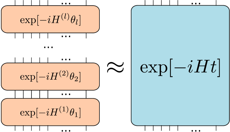
In this paper, we consider the case where the HVA is well approximated by time evolution under a local Hamiltonian, i.e., there are local Hamiltonians $H_{L},H_{R}$ such that $U_{L}\approx e^{-iH_{L}t_{L}}$ and $U_{R}\approx e^{-iH_{R}t_{R}}$ for some $t_{L},t_{R}\geq 0$ (see Fig. 1). With this assumption, we provide strong analytic and numerical arguments that the gradient magnitudes, Eq. (4), only decay at most polynomially in the number of qubits. Although this assumption seems unrealistic, we later show that the HVA with a certain parameter restriction can satisfy this condition.

3 Magnitudes of gradients in Hamiltonian dynamics

In this section, we study the scaling of the gradient when the circuit is given by the time evolution under a time-independent local Hamiltonian. We show that gradients in such circuits do not decay exponentially in both extreme regimes: short- and long-time evolution.

For short-time evolution, we prove a rigorous bound on the time that the gradient preserves its initial magnitudes. Thus, a circuit have large gradients for a proper initial state. On the other hand, for long-time evolution, we combine the universality of quantum thermalization [38, 39, 40] and our numerical results to argue that the gradient does not decay exponentially.

3.1 Gradient scaling for short-time evolution

In this subsection, assuming that (1) a circuit with $N$ qubits is given by $e^{-iHt}$ for a local Hamiltonian $H$ and (2) the initial state has a large gradient with a value of $\Theta(1)$, we prove that there exists $t_{c}=\Theta(1/N)$ such that the circuit maintains the large gradient when the total evolution time is less than $t_{c}$. Our main result is the following proposition:

Proposition 1 (Quantum speed limit of gradients).

For the HVA, the gradient of the cost function is given by

$\displaystyle\partial_{n,m}C=\frac{\partial C}{\partial\theta_{n,m}}=i\operatorname*{Tr}[U_{R}\rho_{0}U_{R}^{\dagger}[H^{(m)},U_{L}^{\dagger}OU_{L}]]$ (6)

where $U_{R}=e^{-iH^{(m-1)}\theta_{n,m-1}}\cdots e^{-iH^{(1)}\theta_{1,1}}$ and $U_{L}=e^{-iH^{(q)}\theta_{p,q}}\cdots e^{-iH^{(m)}\theta_{n,m}}$. Assume that the gradient component, $\partial_{n,m}C$, is non-zero when the circuit is identity, i.e., $|\operatorname*{Tr}[\rho_{0}[H^{(m)},O]]|>0$, and there are local Hamiltonians $H_{L}$, $H_{R}$ such that $U_{L}=e^{-iH_{L}t_{L}}$ and $U_{R}=e^{-iH_{R}t_{R}}$ for some $t_{R},t_{L}\geq 0$. Then,

$\displaystyle\Bigl{|}\frac{\partial C}{\partial\theta_{n,m}}\Bigr{|}\geq|\operatorname*{Tr}[\rho_{0}[H^{(m)},O]]|/2$ (7)

for $t_{R}+t_{L}\leq t_{c}:=|\operatorname*{Tr}[\rho_{0}[H^{(m)},O]]|/(4KC)$, where $K=\max\{\|H_{R}\|,\|H^{(m)}\|\}$, $C=\max\{\|[H^{(m)},O]\|,\|[H_{L},O]\|\}$, and $\|\cdot\|$ is the operator norm.

Proof.

Let

$\displaystyle A(t_{1},t_{2})$
$\displaystyle=i\operatorname*{Tr}[e^{-iH_{R}t_{1}}\rho_{0}e^{iH_{R}t_{1}}[H^{(m)},e^{iH_{L}t_{2}}Oe^{-iH_{L}t_{2}}]].$ (8)

Then

$\displaystyle|A(t_{R},t_{L})-A(0,0)|$
$\displaystyle\qquad\leq\int_{0}^{t_{R}}dt_{1}\Bigl{|}\frac{\partial A(t_{1},0)}{\partial t_{1}}\Bigr{|}+\int_{0}^{t_{L}}dt_{2}\Bigl{|}\frac{\partial A(t_{R},t_{2})}{\partial t_{2}}\Bigr{|}.$ (9)

We further have

$\displaystyle\Bigl{|}\frac{dA(t_{1},0)}{\partial t_{1}}\Bigr{|}$ $\displaystyle=\Bigl{|}\operatorname*{Tr}\bigl{\{}[H_{R},\rho_{0}(t_{1})][H^{(m)},O]\bigr{\}}\Bigr{|}$
$\displaystyle\leq 2\|H_{R}\|\|[H^{(m)},O]\|\leq 2KC,$ (10)

and

$\displaystyle\Bigl{|}\frac{dA(t_{R},t_{2})}{\partial t_{2}}\Bigr{|}$
$\displaystyle=\Bigl{|}\operatorname*{Tr}\bigl{\{}\rho_{0}(t_{R})[H^{(m)},[H_{L},e^{iH_{L}t}Oe^{-iH_{L}t}]]\bigr{\}}\Bigr{|}$
$\displaystyle\leq 2\|H^{(m)}\|\|[H_{L},O]\|\leq 2KC,$ (11)

where $\rho_{0}(t)=e^{-iH_{R}t}\rho_{0}e^{iH_{R}t}$.

Integrating both sides, we have

$\displaystyle|A(t_{R},t_{L})-A(0,0)|\leq 2KC(t_{R}+t_{L}).$ (12)

By entering $t_{R}+t_{L}\leq t_{c}=|A(0,0)|/(4KC)$, we obtain $|A(t_{R},t_{L})-A(0,0)|\leq|A(0,0)|/2$, i.e.,

$\displaystyle A(0,0)-|A(0,0)|/2\leq A(t_{R},t_{L})$
$\displaystyle\qquad\leq A(0,0)+|A(0,0)|/2.$ (13)

We obtain the desired inequality as $A(t_{R},t_{L})\geq A(0,0)/2>0$, if $A(0,0)>0$, and $A(t_{R},t_{L})\leq A(0,0)/2<0$, otherwise. ∎

Let us assume that all of $H^{(m)}$, $H_{L}$, and $H_{R}$ are $k$-local Hamiltonians, where each term acts at most $k$ nearby sites in a given lattice for a constant $k$, and $O$ is a local operator acting on at most a constant number of sites. Under this assumption, which is the case we consider in this paper, we have $t_{c}=\Theta(1/N)$ when $|\operatorname*{Tr}[\rho_{0}[H^{(m)},O]]|=\Theta(1)$. We prove this fact in the rest of the subsection.

For any $k$-local Hamiltonian $H$, we can write

$\displaystyle H=\sum_{i\in\Lambda}h_{i}$ (14)

where $\Lambda=\{1,\cdots,N\}$ is the collection of all sites, and $h_{i}$ is an operator supported by $k$ sites centered at $i$. Formally, we write the support of $h_{i}$ (a set of sites $h_{i}$ acts on) as

$\displaystyle\mathrm{supp}(h_{i})=\{j\in\Lambda:\mathrm{dist}(i,j)\leq k\}$ (15)

where $\mathrm{dist}(i,j)$ is the distance between two sites in the given lattice. We thus have

$\displaystyle\|H\|\leq N\max_{i}\|h_{i}\|,\quad\|[H,O]\|\leq 2s\|O\|\max_{i}\|h_{i}\|$ (16)

for a local operator $O$. Here,

$\displaystyle s=|\{i\in\Lambda:\mathrm{dist}(i,O)\leq k\}|$ (17)

is a constant for a given lattice, where $\mathrm{dist}(i,O)=\min_{j\in\mathrm{supp}(O)}\mathrm{dist}(i,j)$ and $\mathrm{supp}(O)\subset\Lambda$ is the support of $O$. Given that $\|h_{i}\|$, $\|O\|$ are bounded by a constant for a spin system, and $s$ is a constant for a finite-dimensional lattice, we have

$\displaystyle\|H\|=\mathcal{O}(N),\quad\|[H,O]\|=\mathcal{O}(1)$ (18)

for any $k$-local Hamiltonain $H$. We also note that physical Hamiltonians must have $\|H\|=\Theta(N)$, which is a necessary condition to be thermodynamically well-defined. Therefore, we obtain $t_{c}=\Theta(1/N)$ if the circuit has a large initial gradient component, i.e., if there exists $m$ such that $|\operatorname*{Tr}[\rho_{0}[H^{(m)},O]]|=\Theta(1)$.

For example, when $H^{(m)}=\sum_{i}Y_{i}$, $O=Z_{1}$, we have $i\operatorname*{Tr}[\rho_{0}[H^{(m)},O]]=-2$ for $\ket{\psi_{0}}=|+\rangle^{\otimes N}$. Moreover, we have $K=\Theta(N)$ and $C=\Theta(1)$ for Proposition 1, when $H_{R}$ and $H_{L}$ are also $k$-local, which implies $t_{c}=\Theta(1/N)$. Therefore, the gradient component is $\Theta(1)$ for all $t\leq t_{c}$.

While we mostly consider geometrically local Hamiltonians in this paper (i.e., local in a finite-dimensional lattice), our result can be extended to Hamiltonians defined on a general (hyper)graph. Such a complex Hamiltonian appears when a fermionic Hamiltonian is translated to a spin Hamiltonian using, e.g., the Jordan–Wigner transformation (see, e.g., Ref. [7]). These Hamiltonians can have smaller $t_{c}$ because $C=\max\{\|[H^{(m)},O]\|,\|[H_{L},O]\|\}$ in Proposition 1 may scale linearly with $N$. For example, consider a Hamiltonian $H$, each term of which acts on all sites. Namely, we have $H$ given as

$\displaystyle H=\sum_{i=1}^{N}h_{i},$ (19)

where each $h_{i}$ is a Pauli string acting non-trivially on all sites, i.e., $h_{i}\in\{X,Y,Z\}^{\otimes N}$. We still have $\|H\|=\Theta(N)$ for this Hamiltonian. However, for a local operator, $O$, acting on site $i$, we can have $\|[O,H]\|=\Theta(N)$. Thus, applying Proposition 1 to this Hamiltonian yields $t_{c}=\Theta(1/N^{2})$ instead of $\Theta(1/N)$.

3.2 Gradient scaling for long-time evolution

Next, we consider long-time evolution. Following usual arguments for equilibration [41, 40, 42, 43, 44], we assume that a Hamiltonian $H$ follows the non-degenerate energy-gap condition: $E_{i}-E_{j}=E_{k}-E_{l}$ iff $i=k$ and $j=l$; or $i=j$ and $k=l$, where $E_{i}$ is the $i$-th eigenvalue of $H$ with the corresponding eigenvector $\ket{E_{i}}$. With an additional assumption that the Hamiltonian thermalizes [38, 39, 40], in the sense that the observable after equilibration gives a similar value to the thermal average, it is known that the second moment of the Hamiltonian evolution behaves differently from a unitary 2-design [45].

Precisely, Huang et al. [45] considered the saturated value of the out-of-time correlator (OTOC), a widely used measure for detecting quantum chaos. For local Hermitian operators, $O_{i}$ and $O_{j}$ acting on sites $i$ and $j$, respectively, the OTOC is defined by

$\displaystyle\mathrm{OTOC}(O_{i},O_{j})$ $\displaystyle:=\operatorname*{Tr}\Bigl{[}\rho_{0}\bigl{(}UO_{i}U^{\dagger}O_{j}\bigr{)}^{2}\Bigr{]}.$ (20)

Here, $\rho_{0}$ is the initial state, and $U$ is a unitary operator determining the time evolution of the system.

One often considers the infinite temperature initial state given by $\rho_{0}=\operatorname*{\mathds{1}}/2^{N}$ for a system with $N$ qubits. When our unitary operator $U$ forms a 2-design, we obtain

$\displaystyle\mathrm{OTOC}(O_{i},O_{j})$ $\displaystyle=\frac{1}{2^{N}}\operatorname*{Tr}\Bigl{[}UO_{i}U^{\dagger}O_{j}UO_{i}U^{\dagger}O_{j}\Bigr{]}$ (21)
$\displaystyle\xrightarrow{\text{Haar }U}-\frac{2^{N}}{2^{2N}-1},$ (22)

for traceless $O_{i}$ and $O_{j}$ (e.g., local Pauli operators; see, e.g., Ref. [46] for a proof). Namely, $\mathrm{OTOC}(O_{i},O_{j})$ scales inverse exponentially with $N$ in this case. On the other hand, $\mathrm{OTOC}(O_{i},O_{j})$ scales only inverse polynomially with the system size for local Hamiltonian evolution, i.e., when $U=e^{-iHt}$ for a local Hamiltonian $H$ [45]. Such a huge difference mainly comes from the fact that $U=e^{-iHt}$ conserves the energy, i.e., $[H,U]=0$.

Refer to caption
Figure 2: The lower bound $F_{H}(\ket{\psi},H^{(1)},O)$ for $\ket{\psi}=|+\rangle^{\otimes N}$, $H^{(1)}=\sum_{i}Y_{i}$, and $O=\sum_{i}Z_{i}$ averaged over $2^{10}$ randomly generated $k$-local Hamiltonians. Inset: The same results but for Hamiltonians with time-reversal symmetry.

Similarly, one might expect that the variance of gradients saturates to a value that scales only inverse polynomially with $N$ for local Hamiltonian evolution. To see that this is the case, we compute the square of the first element of the gradient (for $\theta_{1,1}$) when $U_{L}=e^{-iH_{L}t}$ and the initial state is given as a pure state $\rho_{0}=\ket{\psi_{0}}\bra{\psi_{0}}$. Then we obtain a lower bound of $(\partial_{\theta_{1,1}}C)^{2}=-\braket{\psi_{0}}{[H^{(1)},O(t)]}{\psi_{0}}^{2}$ where $O(t)=e^{iH_{L}t}Oe^{-iH_{L}t}$ as follows:

Proposition 2.

Assume that $H_{L}$ satisfies the non-degenerate energy-gap condition. Then the long-time average of $-\langle\psi_{0}|[H^{(1)},O(t)]|\psi_{0}\rangle^{2}$ is lower bounded by $F_{H_{L}}(\ket{\psi_{0}},H^{(1)},O)$. Here, $F_{H}(\ket{\psi},G,O)$ is a function given by

$\displaystyle F_{H}(\ket{\psi},G,O)$
$\displaystyle\qquad=2\sum_{ijkl}C_{i}^{*}G_{ij}O_{jk}|C_{k}|^{2}O_{kj}G_{jl}C_{l}$
$\displaystyle\qquad-\sum_{ijkl}C_{i}^{*}O_{ij}G_{jk}C_{k}C_{j}^{*}O_{ji}G_{il}C_{l}$
$\displaystyle\qquad-\sum_{ijkl}C_{i}^{*}G_{ij}O_{jk}C_{k}C_{l}^{*}G_{lk}O_{kj}C_{j},$ (23)

where $C_{i}=\braket{E_{i}}{\psi_{0}}$, $G_{ij}=\braket{E_{i}}{G}{E_{j}}$, and $O_{jk}=\braket{E_{j}}{O}{E_{k}}$. Here, $\ket{E_{i}}$ is the $i$-th eigenstate of $H$.

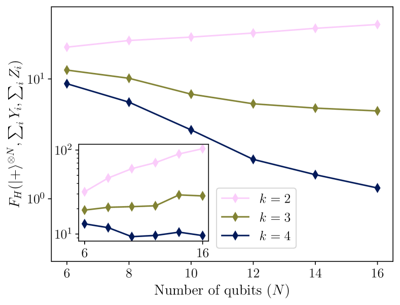
A proof can be found in Appendix B. Unfortunately, we cannot use techniques to analytically compute the OTOC for a maximally mixed initial state $\rho_{0}=\operatorname*{\mathds{1}}/2^{N}$ [45], as we here consider a pure initial state. Instead, we provide numerical evidence that $F_{H}$ does not decay exponentially for translationally invariant local Hamiltonians with and without the time-reversal symmetry. We especially consider time-reversal symmetric Hamiltonians as they are an important subclass of Hamiltonians widely considered for thermalization [47].

After creating a random $k$-local Hamiltonian $H$ (see Appendix C for numerical details), we diagonalize $H$ and compute $F_{H}$ using the obtained eigenstates for the initial state $\ket{\psi}=\ket{+}^{\otimes N}$, $G=\sum_{i}Y_{i}$, and $O=\sum_{i}Z_{i}$. As all observables, the Hamiltonian, and the initial state are translationally-invariant, we can compute $F_{H}$ within the translationally-invariant subspace.

We plot the result in Fig. 2 up to $N=16$ for random Hamiltonians without (main figure) and with (inset) the time-reversal symmetry. For $k=2$, we observe that the lower bound $F_{H}$ does not decay at all in both cases. For $k=3,4$, $F_{H}$ decreases with $N$ for the Hamiltonians without the time-reversal symmetry. Even though it is not conclusive to tell the exact decaying rate of $F_{H}$ from this plot, we strongly believe that it is not exponential from the universality of thermalization dynamics for non-integrable models [38, 39, 40], i.e., if $F_{H}$ for Hamiltonians with the time-reversal symmetry does not decay exponentially, $F_{H}$ for any thermalizing Hamiltonians also does not decay exponentially.

We also recall Ref. [32], which conjectured that the variance of gradients only scales inverse polynomially with the dimension of the dynamical Lie algebra $\mathcal{G}$ spanned by the gate generators, i.e., $\mathcal{G}=\braket{iG_{1},\cdots,iG_{l}}_{\rm Lie}$ where $\braket{\cdot}_{\rm Lie}$ is the Lie closure containing all nested commutators of the listed elements. A reason behind using dynamical Lie algebra is that the algebra generates any arbitrary circuit that the given PQC can express, i.e., there is a $g\in\mathcal{G}$ such that $U(\boldsymbol{\theta})=e^{g}$ for any $\boldsymbol{\theta}$. However, for random Hamiltonians, as in our case, it is more natural to use a vector space of the Hamiltonians (which also generates a unitary operation but not a Lie algebra) instead. As the dimension of $k$-local random Hamiltonians is $\Theta(N)$, the conjecture with a slightly relaxed condition would also indicate that the gradient does not decay exponentially.

We explicitly write down our version of the conjecture, which is also supported by our numerical results, as follows:

Conjecture 1.

Let $V$ be a vector space of local Hamiltonians. Then for any given initial state $\ket{\psi_{0}}$, $G\in V$, and a local operator $O$, we have

$\displaystyle-\int_{\nu\in V}d\nu\braket{\psi_{0}}{[G,e^{i\nu}Oe^{-i\nu}]}{\psi_{0}}^{2}=\frac{1}{\mathrm{poly}(N)}$ (24)

where $d\nu$ is a proper measure for the vector space.

4 Approximating HVA to local Hamiltonian evolution

In the previous section, we argued that a circuit given by the time evolution under a local Hamiltonian does not have barren plateaus. In this section, we find a parameter condition for which the HVA given by Eq. (5) is well approximated by local Hamiltonian evolution. We first interpret the HVA as a unitary operator generated by a time-dependent Hamiltonian. Then, we utilize the Floquet-Magnus (FM) expansion to obtain an effective time-independent Hamiltonian that describes the HVA within a small error.

We here consider each Hamiltonian $H^{(j)}$ satisfying the following conditions: (C1) $H^{(j)}$ is a sum of commuting Pauli strings, (C2) $H^{(j)}$ is $k$-local (each term acts on at most $k$ nearby qubits in a given lattice), and (C3) each Pauli string of $H^{(j)}$ uniquely supports a subset $X\subset\Lambda$ (e.g., $H^{(j)}$ cannot have terms $X_{1}X_{2}$ and $Z_{1}Z_{2}$ simultaneously). In other words, we consider $H^{(j)}$ defined as

$\displaystyle H^{(j)}=\sum_{|X|\leq k}h^{(j)}_{X},$ (25)

where the summation is over all subsets of sites $X\subseteq\Lambda$ whose length is $\leq k$, and $\Lambda=\{1,\cdots,N\}$ is a set of all sites. In addition, $h^{(j)}_{X}$ is a single Pauli string (if there is a term whose support is $X$) or 00 (otherwise), and $[h^{(j)}_{X},h^{(j)}_{Y}]=0$ for all $X,Y\subseteq\Lambda$. As we assume that $H^{(j)}$ is $k$-local, $h^{(j)}_{X}=0$ if $X$ contains any non-nearby sites (i.e., if there are $a,b\in X$ such that the distance between $a$ and $b$ is larger than $k$).

We also define parameters for the FM expansion. First, we define

$\displaystyle H_{\rm max}$ $\displaystyle=\max_{j}\sum_{|X|\leq k}\|h^{(j)}_{X}\|$
$\displaystyle=\max_{j}|\{X\subseteq\Lambda:h^{(j)}_{X}\neq 0\}|,$ (26)

where we obtained the last equality using the fact that $\{h^{(j)}_{X}\}$ are commuting Pauli strings. Thus, $H_{\rm max}$ is the maximum number of terms in $H^{(j)}$. We also introduce a parameter $J$ that upper bounds the local interaction strength

$\displaystyle\max_{j}\sum_{X:X\ni a}\|h^{(j)}_{X}\|\leq J,\qquad\forall a\in\Lambda.$ (27)

As $\{h^{(m)}_{X}\}$ are Pauli strings, we can use

$\displaystyle J=\max_{a\in\Lambda}\max_{j}|\{X:X\ni a\text{ and }h_{X}^{(j)}\neq 0\}|.$ (28)

From the locality of Hamiltonians $\{H^{(j)}\}$, we have $H_{\rm max}=\Theta(N)$ (see discussion below Proposition 1), and $J$ is upper bounded by the number of vertices whose $L^{1}$ distance to the origin is $\leq k$, which is a constant for a finite-dimensional lattice.

We further assume that all parameters $\{\theta_{i,j}\}$ in the HVA are larger than 00. Under this setup, the following Proposition shows that the subcircuits $U_{R}$ and $U_{L}$ of the HVA can be approximated by the time evolution under a few-body Hamiltonian when the sum of parameters is small.

Proposition 3.

For the HVA composed of $H^{(j)}$, given in Eq. 5, we consider a subcircuit $U_{R}=e^{-iH^{(j-1)}\theta_{i,j-1}}\cdots e^{-iH^{(1)}\theta_{1,1}}$. We additionally assume that all $H^{(j)}$ satisfy the conditions (C1-C3) defined above. Then, there is a Hamiltonian $H_{R}^{(n)}$ acting on at most $(n+1)k$-local sites such that

$\displaystyle\Bigl{\|}U_{R}-e^{-iH_{R}^{(n)}t_{R}}\Bigr{\|}$
$\displaystyle\leq 6H_{\rm max}2^{-n_{0}}t_{R}+\frac{2H_{\rm max}(2kJ)^{n+1}}{(n+2)^{2}}(n+1)!t_{R}^{n+2}$ (29)

with $t_{R}=\theta_{1,1}+\cdots+\theta_{i,j-1}$ for all $n\leq n_{0}=\lfloor 1/(32kJt_{R})\rfloor$. Likewise, there is a Hamiltonian $H_{L}^{(n)}$ that approximates $U_{L}=e^{-iH^{(q)}\theta_{p,q}}\cdots e^{-iH^{(j)}\theta_{i,j}}$ with the same error but for $t_{L}=\theta_{i,j}+\cdots+\theta_{p,q}$.

We derive the bound and properties of $H_{R,L}^{(n)}$ in Appendix D. Our derivation is based on the truncated FM expansion rigorously proven in Ref. [48].

The above bound tells us that $U_{R,L}$ can be approximated by local Hamiltonian evolution when $t_{R,L}$ are small. For example, when $t_{R}=\mathcal{O}(1/N)$ and for a constant $n$, the first term in the bound is exponentially small in $N$ and the second term is $\mathcal{O}(1/N^{n+1})$. Then, one may further employ Proposition 1 to get a large gradient, which we summarize as the following theorem:

Theorem 1.

For the HVA [Eq. (5)] and for a local observable $O$ acting on at most $\mathcal{O}(1)$ sites, assume that there exists an initial state $\rho_{0}=\ket{\psi_{0}}\bra{\psi_{0}}$ which gives $g:=|\operatorname*{Tr}[\rho_{0}[H^{(m)},O]]|=\Theta(1)$ regardless of $N$. Then, there is $\tau_{0}=\Theta(1/N)$ such that

$\displaystyle\Bigl{|}\frac{\partial C}{\partial\theta_{n,m}}\Bigr{|}\geq\frac{g}{4}$ (30)

for all $n$, if $\sum_{ij}\theta_{i,j}=t_{L}+t_{R}\leq\tau_{0}$.

The proof can be found in Appendix E.

We provide two remarks on Theorem 1. First, if there exists any constraint with $\tilde{\tau}_{0}$ such that a gradient component is bounded below by a constant for all $\sum_{ij}\theta_{ij}\leq\tilde{\tau}_{0}$, then $\tilde{\tau}_{0}\leq\pi/4$. This is because one can easily find the HVA with suitable $\rho_{0}$ and $O$ which satisfies $|\operatorname*{Tr}[\rho_{0}[H^{(m)},O]]|=\Theta(1)$, but $\partial_{n,m}C=i\operatorname*{Tr}[U(\boldsymbol{\theta})\rho U(\boldsymbol{\theta})^{\dagger}[H^{(m)},O]]=0$ for $\sum_{i,j}\theta_{i,j}=\pi/4$. We provide such an example in Appendix F. This implies that Theorem 1 can be improved at most $\tau_{0}=\Theta(1)$ in our current set-up.

Second, the theorem implies that for any probability distribution $p(\boldsymbol{\theta})$ defined for $\theta_{i,j}\geq 0$ and $\sum_{i,j}\theta_{i,j}\leq\tau_{0}$,

$\displaystyle\int d\boldsymbol{\theta}p(\boldsymbol{\theta})\Bigl{(}\frac{\partial C}{\partial\theta_{n,m}}\Bigr{)}^{2}=\Theta(1),$ (31)

which is much stronger than the non-exponential decay of gradients. If one considers a different condition, e.g., a polynomially decaying gradients under uniformly generated initial parameters, a parameter constraint may be further relaxed. Namely, we open up the possibility that a constraint with $\tau_{1}=\Omega(1)$ exists such that

$\displaystyle\int_{\theta_{i,j}\geq 0,\sum_{i,j}\theta_{i,j}\leq\tau_{1}}\prod_{i,j}d\theta_{i,j}\Bigl{(}\frac{\partial C}{\partial\theta_{n,m}}\Bigr{)}^{2}=\frac{1}{\mathrm{poly}(N)}$ (32)

is satisfied for all $\theta_{i,j}\geq 0$ and $\sum_{i,j}\theta_{i,j}\leq\tau_{1}$. We numerically investigate related scenarios in the following section.

5 Numerical comparison between initialization methods

Theorem 1 tells us that there is $\tau_{0}=\Theta(1/N)$ such that the HVA does not have barren plateaus when the sum of all parameters is less than $\tau_{0}$. Still, the exact value of $\tau_{0}$ for the Theorem is difficult to obtain or can be unrealistically small. Thus, in this subsection, we introduce an initialization method based on Theorem 1 and compare it to the small constant initialization considered in Refs. [49, 50, 51, 52].

We numerically test the following three different initialization methods. (1) Random: complete uniformly random initialization, such that all parameters are from $\mathcal{U}_{[0,2\pi]}$, (2) Constrained: the sum of parameters in each layer is constrained to be $T=c/N$ with a constant $c$, i.e., $\sum_{j}\theta_{i,j}=T$ for all $i$, and (3) Small: $\theta_{i,j}\sim\mathcal{U}_{[0,\epsilon]}$ for a small $\epsilon$ independent to $N$ [49, 50, 51]. For method (2), we show that a relatively large value of $c=\pi/2$ already gives $\Theta(1)$ gradient magnitudes. On the other hand, we observe two different scaling behaviors for the constant small initialization [method (3)]. There is a value $N_{0}$ depending on $p$ and $\epsilon$ such that the gradient magnitudes decay exponentially for $N<N_{0}$ whereas they only decay polynomially for $N>N_{0}$. This observation suggests that there can be another parameter regime in the HVA that does not have barren plateaus.

We use the HVA for the one-dimensional (1D) and two-dimensional (2D) spin-$1/2$ Heisenberg-XYZ models $\mathcal{H}=\sum_{\braket{a,b}}J_{x}X_{a}X_{b}+J_{y}Y_{a}Y_{b}+J_{z}Z_{a}Z_{b}$ to test these methods, which is given by

$\displaystyle\ket{\psi(\boldsymbol{\theta})}$ $\displaystyle=\prod_{i=p}^{1}e^{-i\theta_{i,3}\sum_{\braket{a,b}}Z_{a}Z_{b}}e^{-i\theta_{i,2}\sum_{\braket{a,b}}Y_{a}Y_{b}}$
$\displaystyle\qquad\times e^{-i\theta_{i,1}\sum_{\braket{a,b}}X_{a}X_{b}}\ket{\psi_{0}}$ (33)

where $\braket{a,b}$ are two nearest neighbors and $\ket{\psi_{0}}$ is the Néel state in the given lattice. We use $N$ spins in the periodic boundary condition (a ring) for the one-dimensional model. For the two-dimensional model, we consider a rectangular lattice with the periodic boundary condition (a torus) size of $L_{x}\times L_{y}$. Thus the Néel state in these lattices are given by $\ket{\psi_{0}}=(\ket{\downarrow\uparrow}^{\otimes N/2}+\ket{\uparrow\downarrow}^{\otimes N/2})/\sqrt{2}$ and $[(\ket{\downarrow\uparrow}^{\otimes L_{x}/2}\ket{\uparrow\downarrow}^{\otimes L_{x}/2})^{\otimes L_{y}/2}+(\ket{\uparrow\downarrow}^{\otimes L_{x}/2}\ket{\downarrow\uparrow}^{\otimes L_{x}/2})^{\otimes L_{y}/2}]/\sqrt{2}$ for the 1D and 2D models, respectively.

Refer to caption
Figure 3: (a) Scaling of the gradient square $(\partial_{i,j}C)^{2}$ from the HVA for the 1D Heisenberg-XYZ model with different depths $p$ (see main text for details). Plots show results from the constrained (solid), small (dashed), and completely random (dotted) parameter initializations. We compute $(\partial_{i,j}C)^{2}$ for $2^{10}$ parameters samples from each distribution and plot the averaged results over all samples and gradient components ($i,j$). (b) The same plot as (a) but for the 2D Heisenberg-XYZ model with the lattice size $L_{x}\times L_{y}$. We also see that the results fluctuate for odd and even $L_{y}$ because the 2D Néel state (our initial state) violates the symmetry of the Hamiltonian for odd $L_{y}$. We also compute the relative standard deviation, $r=\sigma(X)/\mathbb{E}[X]$, where $X:=\sum_{ij}(\partial_{i,j}C)^{2}/(3p)$ is the squared partial derivatives averaged over all parameters. Here, the standard deviation and the expectation value are taken over the circuit instances. The values of $r$ for the 1D model with $p=64$ and $N=24$ are given by $0.20$, $0.53$, and $0.13$ for the contained, small, and random initialization, respectively. For the 2D model with $p=64$ and $L_{x}\times L_{y}=4\times 7$, we obtained $r\approx 0.39$ (constrained), $1.02$ (small), $0.11$ (random), respectively.

5.1 Scaling of gradients

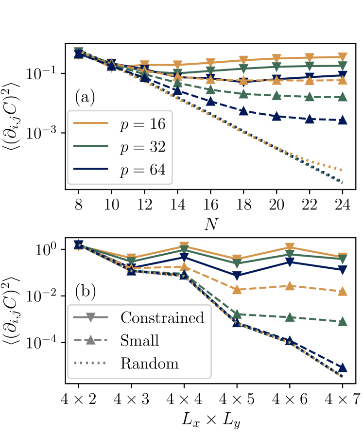
We compute gradients of the cost function with $O=Y_{0}Y_{1}$ (thus $C=\braket{\psi(\boldsymbol{\theta})}{Y_{0}Y_{1}}{\psi(\boldsymbol{\theta})}$) obtained from different initialization methods. For constrained initialization, random values $\tilde{\theta}_{i,j}$ are first sampled from the uniform distribution, i.e., $\tilde{\theta}_{i,j}\sim\mathcal{U}_{[0,2\pi]}$, and then parameters are assigned by normalizing them: $\theta_{i,j}=\tilde{\theta}_{i,j}\times T/(\sum_{j=1}^{3}\tilde{\theta}_{i,j})$ for all $i,j$. This method ensures that $\sum_{j=1}^{3}\theta_{i,j}=T$. We here use $T=\pi/(2N)$. The results are compared to small parameters $\theta_{i,j}\sim\mathcal{U}_{[0,\epsilon]}$ with $\epsilon=0.2$ as well as complete random parameters $\theta_{i,j}\sim\mathcal{U}_{[0,2\pi]}$. For each set of system parameters (size and depth $p$) and the initialization method, we compute all gradient components and plot the averaged squared magnitudes (i.e., we averaged $\langle(\partial_{i,j}C)^{2}\rangle=\sum_{i,j}(\partial_{i,j}C)^{2}/(3p)$ over $2^{10}$ random circuit instances).

The results for the 1D and 2D models are shown in Fig. 3(a) and (b), respectively. The 1D model clearly shows that the magnitudes of gradients do not decay with $N$, i.e., $(\partial_{i,j}C)^{2}\approx\Theta(1)$, for the constrained initialization, which is consistent with Theorem 1. On the other hand, the gradient magnitudes decay exponentially with $N$ when the complete random initialization is used with $p\in[16,32]$. However, we could observe an interesting behavior when parameters are initialized to be small ($\theta_{i,j}\sim\mathcal{U}_{[0,\epsilon]}$). In this case, the gradient decays exponentially up to some $N_{0}$, i.e., for $N\leq N_{0}\approx 18$, but it decays slower after that. One can already see this signature even for the complete random initialization when $p=16$ and $N=24$, where the averaged gradient magnitudes are larger than that from $p\in[32,64]$. We also see similar behaviors for the 2D model, besides the results from each initialization oscillate for odd and even $L_{y}$, since our initial state (2D Néel state) is not fully symmetric for odd $L_{y}$.

Refer to caption
Figure 4: Averaged magnitudes of gradients $\langle(\partial_{i,j}C)^{2}\rangle$ as a function of $\epsilon$. The HVA for the 1D XYZ model with $p=16$ is used. All parameters are samples from the uniform distribution, i.e., $\theta_{i,j}\sim\mathcal{U}_{[0,\epsilon]}$. We observe that there is a value $\epsilon_{0}(N)$ such that the gradient decays exponentially with $N$ only for $\epsilon>\epsilon_{0}(N)$ (colored region). Inset shows the same data but as a function of $\epsilon/\log(N)$. We see the gradient magnitudes saturate after the dashed vertical line, which suggests that $\epsilon_{0}(N)\propto\log N$.

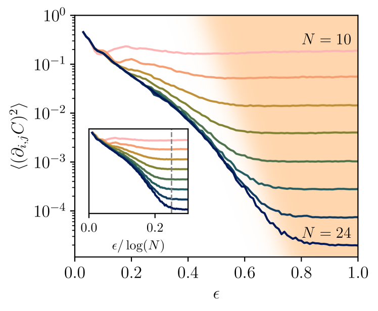
As non-exponential decaying gradients from the small constant initialization have not been clearly reported in previous studies, we explore these phenomena more closely here. We compute the averaged squared gradients using the HVA for the 1D XYZ model with $p=16$ when the circuit parameters are sampled from $\mathcal{U}_{[0,\epsilon]}$ for different values of $N$ and $\epsilon$. We plot the result as a function of $\epsilon$ in Fig. 4. The results show that the magnitudes of gradients saturate to an exponentially small value as $\epsilon$ increases, but the point it saturates, $\epsilon_{0}(N)$, also increases with $N$. For $\epsilon<\epsilon_{0}(N)$, we observe that the gradient does not decay exponentially. This fact also confirms that there can be another parameter regime beyond the one we mainly considered in this paper, which is also free from barren plateaus.

To see how $\epsilon_{0}(N)$ scales with $N$, we plot the same data but as a function of $\epsilon/\log(N)$ (inset). The plot shows that the gradient magnitudes saturate when $\epsilon/\log(N)$ is larger than a constant, which suggests that $\epsilon_{0}(N)\propto\log N$. In general, we expect that there is a relation between $\Upsilon:=\sum_{i,j}\theta_{i,j}$ (which is $\propto p\epsilon$ in this case) in the HVA for a $2$-local Hamiltonian and a random local circuit with depth $\propto\Upsilon$. Such a connection explains the observed behavior as a 1D random local circuit requires its depth larger than $\Theta(\log(N))$ to show exponential decay of gradient magnitudes when the cost function is given by the expectation value of a local observable [16].

We still note that it is less clear whether a small constant parameter initialization [method (3)] gives the same quantitative behavior for the HVAs with more complex Hamiltonians (e.g., 1D $k$-local with $k\geq 3$ or defined in a high-dimensional lattice). In contrast, we expect to have $\Theta(1)$ gradient magnitudes regardless of the dimension with our initialization method [method (2)]. As a detailed investigation of the relation between the HVA and a local random circuit is out of the scope of the current work, we leave it to future work.

Refer to caption
Figure 5: (a) Learning curves from different initialization schemes for the 1D Heisenberg model with $N=20$. We use the circuit ansatz with $p=20$ and the Adam optimizer with the learning rate $\alpha=0.025$. For each iteration, the curves for random and constrained initializations show the averaged results over $32$ different initial parameters. The shaded regions indicate one standard deviation ($[m-\sigma/2,m+\sigma/2]$). Note that results from the constant initialization ($\theta_{i,j}=\pi$) do not vary between instances as there is no randomness in the simulation. The ground state energy $E_{\rm GS}$ is obtained using the exact diagonalization. (b) The same result for the 2D Heisenberg model with $L_{x}\times L_{y}=4\times 6$ lattice. The circuit ansatz with $p=24$ and the Adam optimizer with learning rate $\alpha=0.005$ are used. Results for random and constrained initializations are averaged over $16$ different initial parameters. For optimization, we compute the gradient exactly (without shot noise). Shaded regions are barely visible for the random initialization. This is because the loss function, $\braket{\cal H}$, is not trained at all for most instances. Thus, the loss function preserves its initial value $\braket{\cal H}\approx 0$, which is from the fact that the circuit forms a 2-design for the random initialization.

5.2 Full simulation of variation quantum eigensolver

We now explore whether our initialization improves learning procedures by fully simulating a variational quantum eigensolver (VQE) using the Heisenberg model ($J_{x}=J_{y}=J_{z}=1$). We define the Hamiltonian expectation values as the cost function ($C=\braket{\psi(\boldsymbol{\theta})}{\mathcal{H}}{\psi(\boldsymbol{\theta})}$) and train the circuit using the Adam optimizer [53].

We first simulate the VQEs using exact gradients. Quantum hardware cannot compute exact gradients, as each gradient component should be estimated from the measurement outcomes from shots. However, classical quantum circuit simulators support multiple algorithms to obtain exact gradients. For our simulation, we use the adjoint method [54] implemented in PennyLane [55]. We present learning curves from different parameter initialization methods for the one-dimensional lattices (with learning rate $\alpha=0.025$ and the default values for hyperparameters $\beta_{1}=0.9$ and $\beta_{2}=0.999$) in Fig. 5 (a), which shows that our initialization scheme outperforms other initialization schemes. The completely random parameter initialization fails to find the ground state. This is an expected behavior from the presence of the barren plateaus. On the other hand, initializing all parameters to $\pi$ ($\theta_{i,j}=\pi$ for all $i,j$), which is used in Ref. [31], works but is subject to large initial fluctuations. Generally speaking, such an initialization without randomness is prone to local minima [56]. We also found a similar behavior for the 2D Heisenberg model, shown in Fig. 5(b).

Refer to caption
Figure 6: Converged energies from the VQE for the one-dimensional Heisenberg model with $N=p=16$ as a function of the number of shots. For each number of shots, $n_{\rm shot}\in[2^{7},2^{9},2^{11},2^{13},2^{15},2^{17}]$, we fully simulate the VQE $16$ times. The converged energies $\braket{\mathcal{H}}$ for each independent VQE instance are presented. For the initialization $\theta_{ij}=\pi$, the shot noise is the only source of the randomness. On the other hand, the initial parameters are also random when the constrained parameter initialization is used.

We next compare results from different initialization methods when a finite number of shots is used. We solve the 1D Heisenberg model, but gradients are now estimated using $n_{\rm shot}$ shots.

The gradient with a finite number of shots can be obtained as follows. First, we introduce another PQC with the same shape as the HVA, Eq. (33), but all gates have different parameters. Such a PQC is written as

$\displaystyle\ket{\psi(\boldsymbol{\alpha},\boldsymbol{\beta},\boldsymbol{\gamma})}$
$\displaystyle=\prod_{i=p}^{1}e^{-i\sum_{\braket{a,b}}\gamma_{i,a,b}Z_{a}Z_{b}}e^{-i\sum_{\braket{a,b}}\beta_{i,a,b}Y_{a}Y_{b}}$
$\displaystyle\qquad\times e^{-i\sum_{\braket{a,b}}\alpha_{i,a,b}X_{a}X_{b}}\ket{\psi_{0}}.$ (34)

Compared to Eq. (33), all gates now have independent parameters. Next, we obtain each gradient component using the two-term parameter-shift rule [57, 58]. By defining $f(\boldsymbol{\alpha},\boldsymbol{\beta},\boldsymbol{\gamma})=\braket{\psi(\boldsymbol{\alpha},\boldsymbol{\beta},\boldsymbol{\gamma})}{\mathcal{H}}{\psi(\boldsymbol{\alpha},\boldsymbol{\beta},\boldsymbol{\gamma})}$, we obtain its gradient for $\alpha_{i,a,b}$ as follows:

$\displaystyle\frac{\partial f}{\partial\alpha_{i,a,b}}$ $\displaystyle=\frac{1}{2}\Bigl{[}f\bigl{(}\boldsymbol{\alpha}+\frac{\pi}{2}\boldsymbol{\delta}_{i,a,b},\boldsymbol{\beta},\boldsymbol{\gamma}\bigr{)}$
$\displaystyle\qquad-f\bigl{(}\boldsymbol{\alpha}-\frac{\pi}{2}\boldsymbol{\delta}_{i,a,b},\boldsymbol{\beta},\boldsymbol{\gamma}\bigr{)}\Bigr{]},$ (35)

where $\boldsymbol{\delta}_{i,a,b}$ is a vector components of which is $1$, if the index is $(i,a,b)$, or 00, otherwise. Gradient for $\beta$ and $\gamma$ also can be obtained similarly.

Shot noise is introduced when we estimate $f(\boldsymbol{\alpha},\boldsymbol{\beta},\boldsymbol{\gamma})$. From

$\displaystyle\braket{\mathcal{H}}=\sum_{\braket{a,b}}\braket{X_{a}X_{b}}+\braket{Y_{a}Y_{b}}+\braket{Z_{a}Z_{b}},$ (36)

we can estimate $f=\braket{\psi(\boldsymbol{\alpha},\boldsymbol{\beta},\boldsymbol{\gamma})}{\mathcal{H}}{\psi(\boldsymbol{\alpha},\boldsymbol{\beta},\boldsymbol{\gamma})}$ using the samples of $\psi(\boldsymbol{\alpha},\boldsymbol{\beta},\boldsymbol{\gamma})$ in the $X$, $Y$, and $Z$ bases. For example, let us estimate $\braket{X_{a}X_{b}}$ using $n_{\rm shot}$ samples. We first obtain bitstrings $\{x^{(1)},\cdots,x^{(n_{\rm shot})}\}$ from the probability distribution $p(x)=|\braket{x}{H^{\otimes N}}{\psi(\boldsymbol{\alpha},\boldsymbol{\beta},\boldsymbol{\gamma})}|^{2}$, where each $x^{(i)}\in\{0,1\}^{N}$ is a bitstring with length $N$. Then, each $\braket{X_{a}X_{b}}$ can be estimated using these samples by

$\displaystyle\braket{X_{a}X_{b}}\approx\frac{1}{n_{\rm shot}}\sum_{i=1}^{n_{\rm shot}}(1-2x^{(i)}_{a})(1-x^{(i)}_{b}),$ (37)

where $1-2x^{(i)}_{a}$ is from the fact that $X_{a}$ has the value $1$ if $x^{(i)}_{a}=0$, and $-1$ if $x^{(i)}_{a}=1$. Note that we can use the same set of samples, $\{x^{(1)},\cdots,x^{(n_{\rm shot})}\}$, for all $\braket{X_{a}X_{b}}$. Thus, $f=\braket{\mathcal{H}}$ for each set of parameters is estimated using $3n_{\rm shot}$ samples, and each gradient component is estimated using $6n_{\rm shot}$ samples.

Finally, the gradient of the original HVA, Eq. (33), which shares the parameters between the gates, can be obtained by summing over the gradient components. Namely, we have

$\displaystyle\frac{\partial\braket{\psi(\boldsymbol{\theta})}{\mathcal{H}}{\psi(\boldsymbol{\theta})}}{\theta_{i,1}}=\sum_{\braket{a,b}}\frac{\partial f}{\partial\alpha_{i,a,b}},$ (38)
$\displaystyle\frac{\partial\braket{\psi(\boldsymbol{\theta})}{\mathcal{H}}{\psi(\boldsymbol{\theta})}}{\theta_{i,2}}=\sum_{\braket{a,b}}\frac{\partial f}{\partial\beta_{i,a,b}},$ (39)
$\displaystyle\frac{\partial\braket{\psi(\boldsymbol{\theta})}{\mathcal{H}}{\psi(\boldsymbol{\theta})}}{\theta_{i,3}}=\sum_{\braket{a,b}}\frac{\partial f}{\partial\alpha_{i,a,b}}.$ (40)

Given that the circuit has $3Np$ gates in total, and each gradient component is estimated from $6n_{\rm shot}$ samples, $18Npn_{\rm shot}$ samples are used for each iteration to estimate all gradient components.
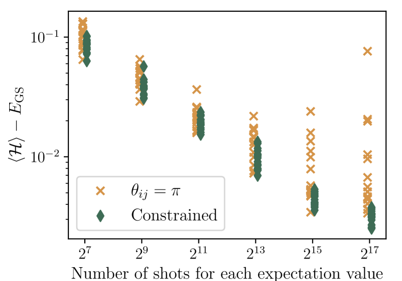
For the HVA with $N=p=16$ [see Eq. (33)], we plot the converged energies after $10^{3}$ iterations from the VQE simulations as a function of $n_{\rm shot}\in[2^{7},2^{9},2^{11},2^{13},2^{15},2^{17}]$ in Fig. 6. While the results show that the best-converged energies from our constrained initialization scheme and $\theta_{ij}=\pi$ are similar, the deviations between instances from our initialization scheme are much smaller. For example, the worst-performing instance for $n_{\rm shot}=2^{15}$ gives $\braket{\mathcal{H}}-E_{\rm GS}\approx 3\times 10^{-2}$ when all parameters are initialized with $\pi$, but that from our initialization is $\approx 6\times 10^{-3}$.

Our parameter constraint can also be imposed throughout the optimization steps (the ansatz itself). When imposed on the ansatz, we can slightly change the cost function to ensure the parameters always follow the constraints. This can be simply done by assigning $\theta_{j,q}=T-\sum_{i=1}^{q-1}\theta_{j,i}$ and replacing the cost function $C$ with $\tilde{C}=[\prod_{i,j}\mathbf{1}(\theta_{j,i})][\prod_{j}\mathbf{1}(T-\sum_{i=1}^{q-1}\theta_{j,i})]C$ where $\mathbf{1}(x)$ is the Heaviside step function. One can see this (piecewise differentiable) cost function (1) restricts all parameters to be larger than 00, and (2) the sum of the parameters in each block is given by $T$ throughout the training.

Still, the constraint-imposed ansatz may not be useful for solving complex problems, as we require $pT$ to be small. Even though the ansatz itself allows a large-depth circuit (e.g., $p=\Theta(N^{2})$ and $T=1/N^{3}$), the Suzuki-Trotter decomposition [59] tells us that such a circuit always can be approximated by a short-depth circuit, i.e., there is another circuit with depth $d=\mathrm{poly}(pT)=\mathrm{poly}(1/N)$ that can express our constrained HVA with a small error. Using the notion of quantum circuit complexity [60, 61, 62, 63], defined by the minimum number of two-qubit gates in any circuit that implements the given unitary, we can say that this ansatz has a small approximate circuit complexity.

Refer to caption
Figure 7: Scaling of the averaged squared gradients $(\partial_{i,j}C)^{2}$ from the repeated ansatz Eq. (41) with (solid) and without (dotted) a parameter constraint. For the parameter-constrained ansatz, we sample parameters under the constraint $\theta_{i,1}+\theta_{i,2}+\theta_{i,3}=\pi/(2N)$. In contrast, $\theta_{i,j}\sim\mathcal{U}_{[0,2\pi]}$ is used for the ansatz without the constraint. The HVA is for the 1D XYZ model with $O=Y_{0}Y_{1}$ with $\tilde{p}=16$ and $r=N^{2}/4$. The results are averaged over $2^{10}$ random parameters.

5.3 Long-time evolution with repeated parameters

To overcome the problem that a simple parameter-constrained ansatz introduced in the previous subsection is not expressive enough, we propose another ansatz with better expressivity. Our solution is to repeat the circuit multiple times instead of adding free parameters. In this case, the circuit is given as

$\displaystyle U(\boldsymbol{\theta})=\Bigl{[}\prod_{i=\tilde{p}}^{1}e^{-iH^{(q)}\theta_{i,q}}\cdots e^{-iH^{(1)}\theta_{i,1}}\Bigr{]}^{r}$ (41)

with the constraint $\sum_{j}\theta_{i,j}=T$. Thus, the circuit has a total of $\tilde{p}qr$ layers but only has $\tilde{p}q$ parameters. This ansatz can be approximated by $e^{-iK(\tilde{p}rT)}$ for a local Hamiltonian $K$ with an error $\mathcal{O}(r(\tilde{p}T)^{n+2})$ when $\tilde{p}T$ is inverse polynomial with $N$ (i.e., $\tilde{p}T=\mathcal{O}(N^{-\gamma})$ for $\gamma>0$). This fact follows from Proposition 3 and $\|U_{1}^{r}-U_{2}^{r}\|\leq r\|U_{1}-U_{2}\|$ which holds for arbitrary $U_{1}$ and $U_{2}$ 222This is from $\|U_{1}^{r}-U_{2}^{r}\|=\|U_{1}U_{1}^{r-1}-U_{1}U_{2}^{r-1}+U_{1}U_{2}^{r-1}-U_{2}U_{2}^{r-1}\|\leq\|U_{1}^{r-1}-U_{2}^{r-1}\|+\|U_{1}-U_{2}\|$, where we used $\|U_{1}\|=\|U_{2}^{r-1}\|=1$..

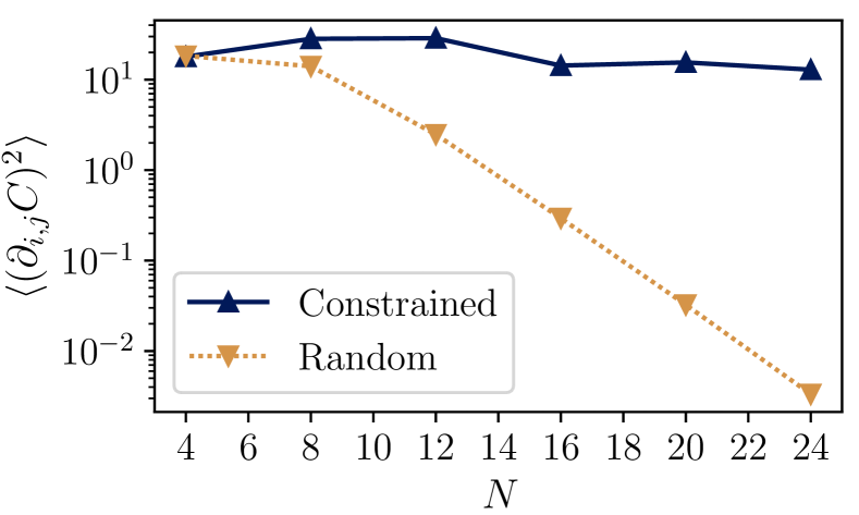
We then further expect that the gradients scale polynomially with $N$ from Conjecture 1 when $\tilde{p}rT$ is sufficiently large enough to equilibrate the system 333Precisely, one also require an ergodicity assumption that resulting Hamiltonians ($K$s) are uniformly distributed over the vector space for random parameters $\theta_{i,j}$.. We also numerically test the gradient scaling of this ansatz for $r=N^{2}/4$, $\tilde{p}=16$, and $T=\pi/(2N)$ using the HVA for the one-dimensional XYZ model in Fig. 7. The plot shows that the gradient does not decay when the parameters are constrained, whereas it decays exponentially otherwise.

We now argue that the repeated ansatz of Eq. (41) (1) can generate sufficiently complex unitary operators and (2) is useful for variational time evolution [33, 34, 35, 36]. The complexity of the circuit directly follows from the observation that the circuit approximates to $e^{-iK(\tilde{p}rT)}$ for a Hamiltonian $K$ with a large $\tilde{p}rT$. It is commonly believed that simulating the long-time evolution of a general local Hamiltonian requires a large depth circuit (which is also formally conjectured in Refs. [64, 65] in terms of quantum circuit complexity). Next, the given ansatz can express the time evolution of a given Hamiltonian $H=\sum_{j=1}^{\tilde{p}}\alpha_{j}H_{j}$. Using the first-order Suzuki-Trotter decomposition, we can write

$\displaystyle e^{-iHt}=(e^{-iHt/r})^{r}\approx\Bigl{[}\prod_{j=\tilde{p}}^{1}e^{-i\alpha_{j}H_{j}t_{0}}\Bigr{]}^{r}$ (42)

with $t_{0}=t/r$ and an error $\mathcal{O}(Nrt_{0}^{2})$. Thus the approximation has an error $\mathcal{O}(1/N)$ if we use $t_{0}=\Theta(1/N)$. As the right-hand side is nothing but Eq. (41) with $T=\sum_{j}\alpha_{j}t_{0}$, the ansatz with $T=\Theta(1/N)$ can approximate $e^{-iHt}$.

6 Conclusion

We studied the scaling behaviors of the gradients in the hamiltonian variational ansatz (HVA) and showed that adding a simple parameter constraint to the ansatz results in large gradients. We demonstrated that the gradient magnitudes scale as $\Theta(1)$ when the circuit is given by short-time evolution and $1/\mathrm{poly}(N)$ when it is given by long-time evolution. For the short-time regime, we provided a rigorous proof based on the rate of the gradient evolution, while we showed numerical evidence based on quantum thermalization [38, 39, 40, 45] for long-time evolution. We then found the parameter constraints for which the HVA can be approximated by short-time as well as long-time evolution under a local Hamiltonian. We further supported our arguments with extensive numerics for up to $28$ qubits, which also consistently showed the correctness of our arguments.

For long-time evolution, our argument is based on the fact that the dynamics generated by thermalizing Hamiltonians are more restricted than unitary 2-designs. Albeit typical Hamiltonians thermalize [44], there are two other important classes of Hamiltonians with different dynamic properties: integrable and many-body localized systems. In contrast to thermalizing systems where information of initial states spreads out through the Hilbert space (but within a subspace preserving the energy), initial information on integrable and many-body localized systems can be easily accessed by simple operators at any time, i.e., their dynamics are even more restrictive than thermalizing Hamiltonians. Given this interesting property, we expect that there could be a different parameter condition that parameterized quantum circuits approximate to integrable or many-body localized systems, which are also free from barren plateaus.

For example, it is known that the out-of-time correlator of many-body localized systems does not decay exponentially with the system size for particular choices of observables and initial states (see, e.g., Refs. [66, 67, 68]). Following the arguments in Sec. 3.2, we hope to find a class of parameterized quantum circuits that approximate to a many-body localized system and have large gradients. On the other hand, Ref. [32] showed that the dynamic Lie algebra $\mathcal{G}$ generated by the HVA for the XXZ model ($J_{x}=J_{y}$) can have a small dimension, i.e., the Lie algebra $\langle i\sum_{i}(X_{i}X_{i+1}+Y_{i}Y_{i+1}),i\sum_{i}Z_{i}Z_{i+1}\rangle_{\rm Lie}$, has a small dimension. As the XXZ model is solvable by the Bethe ansatz (thus integrable), we believe that a fundamental connection exists between the low-dimensional dynamical Lie algebra, the integrability of the system, and large gradients. Such a connection might be studied in future work.

This paper did not consider incoherent noise, which prevails in noisy quantum devices. This type of noise is known to be another source of barren plateaus [69]. When the circuit is short enough, we believe that our initialization schemes can help compensate for the vanishing gradients from the incoherent noises. Still, how the strength of the noise, the circuit depth, and the initialization schemes interplay in general is another big question that requires a separate study. Since this is important for practical applications of variational quantum algorithms, further research on the effect of incoherent noises is necessary.

Acknowledgements

The authors thank Modjtaba Shokrian Zini for helpful discussions and David Wierichs, Maria Schuld, and Joseph Bowles for valuable comments. This research used resources of the National Energy Research Scientific Computing Center, a DOE Office of Science User Facility supported by the Office of Science of the U.S. Department of Energy under Contract No. DE-AC02-05CH11231 using NERSC award NERSC DDR-ERCAP0025705. Numerical simulations were performed using PennyLane [55] software package with Lightning [70] and Lightning-GPU [71] plugins. The source code used for simulations is available in Ref. [72].

References

  • [1] Frank Arute, Kunal Arya, Ryan Babbush, Dave Bacon, Joseph C Bardin, Rami Barends, Rupak Biswas, Sergio Boixo, Fernando GSL Brandao, David A Buell, et al. “Quantum supremacy using a programmable superconducting processor”. Nature 574, 505–510 (2019).
  • [2] Han-Sen Zhong, Hui Wang, Yu-Hao Deng, Ming-Cheng Chen, Li-Chao Peng, Yi-Han Luo, Jian Qin, Dian Wu, Xing Ding, Yi Hu, et al. “Quantum computational advantage using photons”. Science 370, 1460–1463 (2020).
  • [3] Lars S Madsen, Fabian Laudenbach, Mohsen Falamarzi Askarani, Fabien Rortais, Trevor Vincent, Jacob FF Bulmer, Filippo M Miatto, Leonhard Neuhaus, Lukas G Helt, Matthew J Collins, et al. “Quantum computational advantage with a programmable photonic processor”. Nature 606, 75–81 (2022).
  • [4] John Preskill. “Quantum computing in the NISQ era and beyond”. Quantum 2, 79 (2018).
  • [5] Edward Farhi, Jeffrey Goldstone, and Sam Gutmann. “A quantum approximate optimization algorithm” (2014). arXiv:1411.4028.
  • [6] Alberto Peruzzo, Jarrod McClean, Peter Shadbolt, Man-Hong Yung, Xiao-Qi Zhou, Peter J Love, Alán Aspuru-Guzik, and Jeremy L O’Brien. “A variational eigenvalue solver on a photonic quantum processor”. Nat. Comm. 5, 1–7 (2014).
  • [7] Dave Wecker, Matthew B Hastings, and Matthias Troyer. “Progress towards practical quantum variational algorithms”. Phys. Rev. A 92, 042303 (2015).
  • [8] Abhinav Kandala, Antonio Mezzacapo, Kristan Temme, Maika Takita, Markus Brink, Jerry M Chow, and Jay M Gambetta. “Hardware-efficient variational quantum eigensolver for small molecules and quantum magnets”. Nature 549, 242–246 (2017).
  • [9] Stuart Hadfield, Zhihui Wang, Bryan O’Gorman, Eleanor G Rieffel, Davide Venturelli, and Rupak Biswas. “From the quantum approximate optimization algorithm to a quantum alternating operator ansatz”. Algorithms 12, 34 (2019).
  • [10] Maria Schuld, Ilya Sinayskiy, and Francesco Petruccione. “An introduction to quantum machine learning”. Contemporary Physics 56, 172–185 (2015).
  • [11] Jacob Biamonte, Peter Wittek, Nicola Pancotti, Patrick Rebentrost, Nathan Wiebe, and Seth Lloyd. “Quantum machine learning”. Nature 549, 195–202 (2017).
  • [12] Maria Schuld and Nathan Killoran. “Quantum machine learning in feature Hilbert spaces”. Phys. Rev. Lett. 122, 040504 (2019).
  • [13] Yunchao Liu, Srinivasan Arunachalam, and Kristan Temme. “A rigorous and robust quantum speed-up in supervised machine learning”. Nat. Phys. 17, 1013–1017 (2021).
  • [14] Marco Cerezo, Andrew Arrasmith, Ryan Babbush, Simon C Benjamin, Suguru Endo, Keisuke Fujii, Jarrod R McClean, Kosuke Mitarai, Xiao Yuan, Lukasz Cincio, et al. “Variational quantum algorithms”. Nat. Rev. Phys. 3, 625–644 (2021).
  • [15] Jarrod R McClean, Sergio Boixo, Vadim N Smelyanskiy, Ryan Babbush, and Hartmut Neven. “Barren plateaus in quantum neural network training landscapes”. Nat. Comm. 9, 1–6 (2018).
  • [16] Marco Cerezo, Akira Sone, Tyler Volkoff, Lukasz Cincio, and Patrick J Coles. “Cost function dependent barren plateaus in shallow parametrized quantum circuits”. Nat. Comm. 12, 1–12 (2021).
  • [17] Zoë Holmes, Kunal Sharma, Marco Cerezo, and Patrick J Coles. “Connecting ansatz expressibility to gradient magnitudes and barren plateaus”. PRX Quantum 3, 010313 (2022).
  • [18] Sepp Hochreiter and Jürgen Schmidhuber. “Long short-term memory”. Neural computation 9, 1735–1780 (1997).
  • [19] Xavier Glorot, Antoine Bordes, and Yoshua Bengio. “Deep sparse rectifier neural networks”. In Proceedings of the fourteenth international conference on artificial intelligence and statistics. Pages 315–323. JMLR Workshop and Conference Proceedings (2011). url: https://proceedings.mlr.press/v15/glorot11a.html.
  • [20] Xavier Glorot and Yoshua Bengio. “Understanding the difficulty of training deep feedforward neural networks”. In Proceedings of the thirteenth international conference on artificial intelligence and statistics. Pages 249–256. JMLR Workshop and Conference Proceedings (2010). url: https://proceedings.mlr.press/v9/glorot10a.html.
  • [21] Kaiming He, Xiangyu Zhang, Shaoqing Ren, and Jian Sun. “Delving deep into rectifiers: Surpassing human-level performance on imagenet classification”. In Proceedings of the IEEE international conference on computer vision. Pages 1026–1034.  (2015).
  • [22] Kaining Zhang, Min-Hsiu Hsieh, Liu Liu, and Dacheng Tao. “Toward trainability of quantum neural networks” (2020). arXiv:2011.06258.
  • [23] Tyler Volkoff and Patrick J Coles. “Large gradients via correlation in random parameterized quantum circuits”. Quantum Science and Technology 6, 025008 (2021).
  • [24] Arthur Pesah, Marco Cerezo, Samson Wang, Tyler Volkoff, Andrew T Sornborger, and Patrick J Coles. “Absence of barren plateaus in quantum convolutional neural networks”. Phys. Rev. X 11, 041011 (2021).
  • [25] Xia Liu, Geng Liu, Jiaxin Huang, Hao-Kai Zhang, and Xin Wang. “Mitigating barren plateaus of variational quantum eigensolvers” (2022). arXiv:2205.13539.
  • [26] Edward Grant, Leonard Wossnig, Mateusz Ostaszewski, and Marcello Benedetti. “An initialization strategy for addressing barren plateaus in parametrized quantum circuits”. Quantum 3, 214 (2019).
  • [27] Nishant Jain, Brian Coyle, Elham Kashefi, and Niraj Kumar. “Graph neural network initialisation of quantum approximate optimisation”. Quantum 6, 861 (2022).
  • [28] Kaining Zhang, Liu Liu, Min-Hsiu Hsieh, and Dacheng Tao. “Escaping from the barren plateau via gaussian initializations in deep variational quantum circuits”. In Advances in Neural Information Processing Systems. Volume 35, pages 18612–18627.  (2022). url: https://doi.org/10.48550/arXiv.2203.09376.
  • [29] Antonio A. Mele, Glen B. Mbeng, Giuseppe E. Santoro, Mario Collura, and Pietro Torta. “Avoiding barren plateaus via transferability of smooth solutions in a Hamiltonian variational ansatz”. Phys. Rev. A 106, L060401 (2022).
  • [30] Manuel S Rudolph, Jacob Miller, Danial Motlagh, Jing Chen, Atithi Acharya, and Alejandro Perdomo-Ortiz. “Synergistic pretraining of parametrized quantum circuits via tensor networks”. Nature Communications 14, 8367 (2023).
  • [31] Roeland Wiersema, Cunlu Zhou, Yvette de Sereville, Juan Felipe Carrasquilla, Yong Baek Kim, and Henry Yuen. “Exploring entanglement and optimization within the Hamiltonian variational ansatz”. PRX Quantum 1, 020319 (2020).
  • [32] Martin Larocca, Piotr Czarnik, Kunal Sharma, Gopikrishnan Muraleedharan, Patrick J Coles, and M Cerezo. “Diagnosing barren plateaus with tools from quantum optimal control”. Quantum 6, 824 (2022).
  • [33] Ying Li and Simon C Benjamin. “Efficient variational quantum simulator incorporating active error minimization”. Phys. Rev. X 7, 021050 (2017).
  • [34] Xiao Yuan, Suguru Endo, Qi Zhao, Ying Li, and Simon C Benjamin. “Theory of variational quantum simulation”. Quantum 3, 191 (2019).
  • [35] Cristina Cirstoiu, Zoe Holmes, Joseph Iosue, Lukasz Cincio, Patrick J Coles, and Andrew Sornborger. “Variational fast forwarding for quantum simulation beyond the coherence time”. npj Quantum Information 6, 1–10 (2020).
  • [36] Sheng-Hsuan Lin, Rohit Dilip, Andrew G Green, Adam Smith, and Frank Pollmann. “Real-and imaginary-time evolution with compressed quantum circuits”. PRX Quantum 2, 010342 (2021).
  • [37] Conor Mc Keever and Michael Lubasch. “Classically optimized hamiltonian simulation”. Phys. Rev. Res. 5, 023146 (2023).
  • [38] Josh M Deutsch. “Quantum statistical mechanics in a closed system”. Phys. Rev. A 43, 2046 (1991).
  • [39] Mark Srednicki. “Chaos and quantum thermalization”. Phys. Rev. E 50, 888 (1994).
  • [40] Marcos Rigol, Vanja Dunjko, and Maxim Olshanii. “Thermalization and its mechanism for generic isolated quantum systems”. Nature 452, 854–858 (2008).
  • [41] Peter Reimann. “Foundation of statistical mechanics under experimentally realistic conditions”. Phys. Rev. Lett. 101, 190403 (2008).
  • [42] Noah Linden, Sandu Popescu, Anthony J Short, and Andreas Winter. “Quantum mechanical evolution towards thermal equilibrium”. Phys. Rev. E 79, 061103 (2009).
  • [43] Anthony J Short. “Equilibration of quantum systems and subsystems”. New Journal of Physics 13, 053009 (2011).
  • [44] Christian Gogolin and Jens Eisert. “Equilibration, thermalisation, and the emergence of statistical mechanics in closed quantum systems”. Reports on Progress in Physics 79, 056001 (2016).
  • [45] Yichen Huang, Fernando GSL Brandão, Yong-Liang Zhang, et al. “Finite-size scaling of out-of-time-ordered correlators at late times”. Phys. Rev. Lett. 123, 010601 (2019).
  • [46] Daniel A Roberts and Beni Yoshida. “Chaos and complexity by design”. Journal of High Energy Physics 2017, 1–64 (2017).
  • [47] Hyungwon Kim, Tatsuhiko N Ikeda, and David A Huse. “Testing whether all eigenstates obey the eigenstate thermalization hypothesis”. Phys. Rev. E 90, 052105 (2014).
  • [48] Tomotaka Kuwahara, Takashi Mori, and Keiji Saito. “Floquet–Magnus theory and generic transient dynamics in periodically driven many-body quantum systems”. Annals of Physics 367, 96–124 (2016).
  • [49] David Wierichs, Christian Gogolin, and Michael Kastoryano. “Avoiding local minima in variational quantum eigensolvers with the natural gradient optimizer”. Phys. Rev. Research 2, 043246 (2020).
  • [50] Chae-Yeun Park. “Efficient ground state preparation in variational quantum eigensolver with symmetry breaking layers” (2021). arXiv:2106.02509.
  • [51] Jan Lukas Bosse and Ashley Montanaro. “Probing ground-state properties of the kagome antiferromagnetic heisenberg model using the variational quantum eigensolver”. Phys. Rev. B 105, 094409 (2022).
  • [52] Joris Kattemölle and Jasper van Wezel. “Variational quantum eigensolver for the heisenberg antiferromagnet on the kagome lattice”. Phys. Rev. B 106, 214429 (2022).
  • [53] Diederik P. Kingma and Jimmy Ba. “Adam: A method for stochastic optimization”. In 3rd International Conference on Learning Representations, ICLR 2015, San Diego, CA, USA, May 7-9, 2015, Conference Track Proceedings.  (2015). url: https://doi.org/10.48550/arXiv.1412.6980.
  • [54] Tyson Jones and Julien Gacon. “Efficient calculation of gradients in classical simulations of variational quantum algorithms” (2020). arXiv:2009.02823.
  • [55] Ville Bergholm, Josh Izaac, Maria Schuld, Christian Gogolin, Shahnawaz Ahmed, Vishnu Ajith, M. Sohaib Alam, Guillermo Alonso-Linaje, et al. “Pennylane: Automatic differentiation of hybrid quantum-classical computations” (2018). arXiv:1811.04968.
  • [56] Lodewyk FA Wessels and Etienne Barnard. “Avoiding false local minima by proper initialization of connections”. IEEE Transactions on Neural Networks 3, 899–905 (1992).
  • [57] Kosuke Mitarai, Makoto Negoro, Masahiro Kitagawa, and Keisuke Fujii. “Quantum circuit learning”. Phys. Rev. A 98, 032309 (2018).
  • [58] Maria Schuld, Ville Bergholm, Christian Gogolin, Josh Izaac, and Nathan Killoran. “Evaluating analytic gradients on quantum hardware”. Phys. Rev. A 99, 032331 (2019).
  • [59] Masuo Suzuki. “General theory of fractal path integrals with applications to many-body theories and statistical physics”. Journal of Mathematical Physics 32, 400–407 (1991).
  • [60] Michael A. Nielsen. “A geometric approach to quantum circuit lower bounds” (2005). arXiv:quant-ph/0502070.
  • [61] Michael A Nielsen, Mark R Dowling, Mile Gu, and Andrew C Doherty. “Quantum computation as geometry”. Science 311, 1133–1135 (2006).
  • [62] Douglas Stanford and Leonard Susskind. “Complexity and shock wave geometries”. Phys. Rev. D 90, 126007 (2014).
  • [63] Jonas Haferkamp, Philippe Faist, Naga BT Kothakonda, Jens Eisert, and Nicole Yunger Halpern. “Linear growth of quantum circuit complexity”. Nat. Phys. 18, 528–532 (2022).
  • [64] Adam R Brown, Leonard Susskind, and Ying Zhao. “Quantum complexity and negative curvature”. Phys. Rev. D 95, 045010 (2017).
  • [65] Adam R Brown and Leonard Susskind. “Second law of quantum complexity”. Phys. Rev. D 97, 086015 (2018).
  • [66] Yu Chen. “Universal logarithmic scrambling in many body localization” (2016). arXiv:1608.02765.
  • [67] Ruihua Fan, Pengfei Zhang, Huitao Shen, and Hui Zhai. “Out-of-time-order correlation for many-body localization”. Science Bulletin 62, 707–711 (2017).
  • [68] Juhee Lee, Dongkyu Kim, and Dong-Hee Kim. “Typical growth behavior of the out-of-time-ordered commutator in many-body localized systems”. Phys. Rev. B 99, 184202 (2019).
  • [69] Samson Wang, Enrico Fontana, Marco Cerezo, Kunal Sharma, Akira Sone, Lukasz Cincio, and Patrick J Coles. “Noise-induced barren plateaus in variational quantum algorithms”. Nat. Comm. 12, 6961 (2021).
  • [70] “PennyLane–Lightning plugin https://github.com/PennyLaneAI/pennylane-lightning” (2023).
  • [71] “PennyLane–Lightning-GPU plugin https://github.com/PennyLaneAI/pennylane-lightning-gpu” (2023).
  • [72] “GitHub repository https://github.com/XanaduAI/hva-without-barren-plateaus” (2023).
  • [73] Wilhelm Magnus. “On the exponential solution of differential equations for a linear operator”. Commun. Pure. Appl. Math. 7, 649–673 (1954).
  • [74] Dmitry Abanin, Wojciech De Roeck, Wen Wei Ho, and François Huveneers. “A rigorous theory of many-body prethermalization for periodically driven and closed quantum systems”. Commun. Math. Phys. 354, 809–827 (2017).
\onecolumngrid

Appendix A Big-$O$ and related notations

In the main text, we have used big-$O$ and related notations. This appendix formally defines these notations as follows:

  • $f(n)=\mathcal{O}(g(n))$ if there exist $n_{0}\in\mathbb{N}^{+}$ and $c\in\mathbb{R}^{+}$ such that $f(n)\leq cg(n)$ for all $n\geq n_{0}$.

  • $f(n)=\Omega(g(n))$ if there exist $N_{0}\in\mathbb{N}^{+}$ and $c\in\mathbb{R}^{+}$ such that $f(n)\geq cg(n)$ for all $n\geq n_{0}$.

  • $f(n)=\Theta(g(n))$ if $f(n)=\mathcal{O}(g(n))$ and $f(n)=\Omega(g(n))$.

Appendix B Long-time average of the variance of gradients in the Hamiltonian dynamics

In this appendix, we prove Proposition 2, which gives the lower bound of a long-time average of the squared gradient for a Hamiltonian evolution. Direct computation of $\langle\psi_{0}|i[G,O(t)]|\psi_{0}\rangle^{2}$ gives

$\displaystyle\langle\psi_{0}|i[G,O(t)]|\psi_{0}\rangle^{2}$ $\displaystyle=-\Bigl{[}\braket{\psi_{0}}{Ge^{iHt}Oe^{-iHt}}{\psi_{0}}-\braket{\psi_{0}}{e^{iHt}Oe^{-iHt}G}{\psi_{0}}\Bigr{]}^{2}$ (B.1)
$\displaystyle=-\Bigl{[}\sum_{ijk}C_{i}^{*}G_{ij}e^{i(E_{j}-E_{k})t}O_{jk}C_{k}-\sum_{lmn}C_{l}^{*}e^{i(E_{l}-E_{m})t}O_{lm}G_{mn}C_{n}\Bigr{]}^{2}$ (B.2)
$\displaystyle=-\sum_{ijki^{\prime}j^{\prime}k^{\prime}}C_{i}^{*}G_{ij}e^{i(E_{j}-E_{k})t}O_{jk}C_{k}C_{i^{\prime}}^{*}G_{i^{\prime}j^{\prime}}e^{i(E_{j^{\prime}}-E_{k^{\prime}})t}O_{j^{\prime}k^{\prime}}C_{k^{\prime}}$
$\displaystyle\qquad-\sum_{lmnl^{\prime}m^{\prime}n^{\prime}}C_{l}^{*}e^{i(E_{l}-E_{m})t}O_{lm}G_{mn}C_{n}C_{l^{\prime}}^{*}e^{i(E_{l^{\prime}}-E_{m^{\prime}})t}O_{l^{\prime}m^{\prime}}G_{m^{\prime}n^{\prime}}C_{n^{\prime}}$
$\displaystyle\qquad+2\sum_{ijklmn}C_{i}^{*}G_{ij}e^{i(E_{j}-E_{k})t}O_{jk}C_{k}C_{l}^{*}e^{i(E_{l}-E_{m})t}O_{lm}G_{mn}C_{n}$ (B.3)

where $C_{i}=\braket{E_{i}}{\psi_{0}}$, $G_{ij}=\braket{E_{i}}{G}{E_{j}}$, and $O_{jk}=\braket{E_{j}}{O}{E_{k}}$.

We assume that the Hamiltonian $H$ satisfies the non-degenerate energy-gap condition, i.e.,

$\displaystyle E_{i}-E_{j}=E_{k}-E_{l}\text{\quad iff \quad}\begin{cases}&i=k\text{ and }j=l\\ &i=j\text{ and }k=l\end{cases}.$ (B.4)

Under this condition, averaging Eq. (B.3) over time yields

$\displaystyle\lim_{T\rightarrow\infty}\frac{1}{T}\int_{0}^{T}dt\Bigl{\{}-\langle[G,O(t)]\rangle^{2}\Bigr{\}}$ $\displaystyle=2\sum_{ijkn}C_{i}^{*}G_{ij}O_{jk}|C_{k}|^{2}O_{kj}G_{jn}C_{n}-\sum_{lmnn^{\prime}}C_{l}^{*}O_{lm}G_{mn}C_{n}C_{m}^{*}O_{ml}G_{ln^{\prime}}C_{n^{\prime}}$
$\displaystyle\qquad-\sum_{ijkl}C_{i}^{*}G_{ij}O_{jk}C_{k}C_{l}^{*}G_{lk}O_{kj}C_{j}-\braket{\psi}{[G,\tilde{O}]}{\psi}^{2}$ (B.5)
$\displaystyle=F_{H}(\psi,G,O)-\braket{\psi}{[G,\tilde{O}]}{\psi}^{2}\geq F_{H}(\psi,G,O)$ (B.6)

where $\tilde{O}=\sum_{j}O_{jj}\ket{E_{j}}\bra{E_{j}}$. As $\braket{\psi}{[G,\tilde{O}]}{\psi}$ is purely imaginary, we obtain the last inequality. The inequality in the main text is then obtained by changing the summation indices.

We also note that the eigenstate thermalization hypothesis [38, 39, 40] suggests that the last term, $\braket{\psi}{[G,\tilde{O}]}{\psi}^{2}$, is exponentially small in $N$.

Appendix C Generating random Hamiltonians

In the main text, we numerically observed the scaling behaviors of gradient magnitudes using random Hamiltonians. Here, we describe detailed steps to generate such random $k$-local Hamiltonians. For a given $k$, we first create a set of terms $S=\{\sigma^{1}_{a_{1}}\sigma^{2}_{a_{2}}\cdots\sigma^{k}_{a_{k}}\}$ where each $\sigma^{i}_{a_{i}}$ is one of the the Pauli matrices at site $i$ ($\{I_{i},X_{i},Y_{i},Z_{i}\}$) where $a_{k}\in\{0,1,2,3\}$ for all $k$. We then remove terms duplicated under translation. For example, as $X\otimes I\otimes I$, $I\otimes X\otimes I$, and $I\otimes I\otimes X$ generate the same terms under translation, we only keep one of them. We then construct a random Hamiltonian $H=\sum_{s\in S}c_{s}\sum_{n=1}^{N}\mathsf{T}^{n}s$, where the coefficients $c_{s}$ are samples from the normal distribution $\mathcal{N}(0,1)$ and $\mathsf{T}$ is the translation operator ($\mathsf{T}\sigma^{i}_{a}=\sigma^{i+1}_{a}$). We also generate random time-reversal symmetric Hamiltonians ($H^{*}=H$) using the same method but removing purely imaginary operators (that contain odd numbers of Pauli-$Y$s) from $S$.

Appendix D Approximation of the HVA from the truncated Floquet-Magnus expansion

In this appendix, we prove Proposition 3 using the truncated Floquet-Magnus (FM) expansion. The FM expansion [73] provides a time-independent effective Hamiltonian for a unitary evolution from a time-dependent Hamiltonian. While this expansion diverges for a general many-body Hamiltonian, recent works [48, 74] have shown that we can still use the expansion after truncating high-order terms.

D.1 Truncated Floquet-Magnus expansion

Let us introduce the truncated FM expansion following the notation in Ref. [48]. We consider a system defined on a lattice with $N$ spins where each spin is labeled by $i=1$ to $N$. The set of all spins is denoted by $\Lambda=\{1,\cdots,N\}$. We consider a time-dependent Hamiltonian $H(t)$ defined for $0\leq t\leq\tau$. We decompose the Hamiltonian into $H(t)=H_{0}+V(t)$ where $H_{0}$ is the time-independent part and $V(t)$ is the remaining time-dependent part. Both parts have at most $k$-body interactions (we do not impose geometric locality yet). We then write the Hamiltonian terms as

$\displaystyle H_{0}=\sum_{|X|\leq k}h_{X},\qquad V(t)=\sum_{|X|\leq k}v_{X}(t),$ (D.7)

where $X$ is all possible subsets of $\Lambda$ and $|X|$ is the number of elements in the set.

We introduce a parameter $J$ that upper bounds local interaction strength and some additional parameters for the expansion:

$\displaystyle\sum_{X:X\ni i}(\|h_{X}\|+\|v_{X}(t)\|)\leq J\quad\forall i\in\Lambda,\qquad V_{0}:=\sum_{|X|\leq k}\frac{1}{\tau}\int_{0}^{\tau}\|v_{X}(t)\|dt,\qquad\lambda:=2kJ.$ (D.8)

Under this setting, we are interested in the Floquet Hamiltonian $H_{F}$ defined as

$\displaystyle e^{-iH_{F}\tau}:=\mathcal{T}[e^{-i\int_{0}^{\tau}H(t)dt}],$ (D.9)

where $\mathcal{T}[\cdot]$ is the time-ordering operator. One can expand the Floquet Hamiltonian as $H_{F}=\sum_{n=0}^{\infty}\tau^{n}\Omega_{n}$ where the terms $\{\Omega_{n}\}_{n=0}^{\infty}$ are given by the FM expansion as follows:

$\displaystyle\Omega_{n}$ $\displaystyle=\frac{1}{(n+1)^{2}}\sum_{\sigma\in S_{n+1}}(-1)^{n-\omega(\sigma)}\frac{\omega(\sigma)!(n-\omega(\sigma))!}{n!}$
$\displaystyle\qquad\times\frac{1}{i^{n}\tau^{n+1}}\int_{0}^{\tau}dt_{n+1}\cdots\int_{0}^{t_{3}}dt_{2}\int_{0}^{t_{2}}dt_{1}[H(t_{\sigma(n+1))},[H(t_{\sigma(n)}),\cdots,[H(t_{\sigma(2)}),H(t_{\sigma(1)})]\cdots]],$ (D.10)

where $S_{n+1}$ is the permutation group on $n+1$ letters, $\omega(\sigma)=\sum_{i=1}^{n}\mathbf{1}[\sigma(i+1)-\sigma(i)]$, and $\mathbf{1}(x)$ is the Heaviside step function. In our setup, where the Hamiltonian terms have at most $k$-body interactions, $\Omega_{n}$ has at most $(n+1)k$-body interactions. We further have the following upper bound for $\Omega_{n}$ (Lemma 1 in Ref. [48]):

$\displaystyle\|\Omega_{n}\|\leq\frac{2V_{0}\lambda^{n}}{(n+1)^{2}}n!=:\overline{\Omega}_{n}.$ (D.11)

One can see that the convergence condition $\|\Omega_{n+1}\|\tau^{n+1}<\|\Omega_{n}\|\tau^{n}$ only holds up to $n\approx(\lambda\tau)^{-1}$. Indeed, the FM expansion diverges for a many-body Hamiltonian unless $\tau$ also scales with $N$. Even though this fact suggests that the FM expansion might not be useful, it turned out that one can still use a truncated series $H_{F}^{(n)}:=\sum_{m=0}^{n}\tau^{m}\Omega_{m}$ to describe long-time dynamics accurately:

Theorem D.1 (Theorem 1 in Ref. [48]).

With our parameters in Eq. (D.8) and additional condition $\tau\leq 1/(4\lambda)$, the time evolution under the time-dependent Hamiltonian $H(t)=H_{0}+V(t)$ is close to that generated by the truncated Floquet Hamiltonian $H_{F}^{(n_{0})}=\sum_{m=0}^{n_{0}}\Omega_{m}\tau^{m}$ with

$\displaystyle n_{0}:=\left\lfloor\frac{1}{16\lambda\tau}\right\rfloor,$ (D.12)

in the sense that

$\displaystyle\|e^{-iH_{F}\tau}-e^{-iH_{F}^{(n_{0})}\tau}\|\leq 6V_{0}\tau 2^{-n_{0}}.$ (D.13)

However, as $n_{0}$ increases with $N$, if $\tau\sim N^{-\alpha}$ for a positive $\alpha$, the interaction range of $H_{F}^{(n_{0})}$ increases with $N$. As we want strict locality in our Hamiltonian (it must be $k^{\prime}$-local for a constant $k^{\prime}$), a bound for $H_{F}^{(n)}$ for a fixed $n$ should be useful, which is provided by the following Corollary.

Corollary D.1 (Corollary 1 in Ref. [48]).

Under the same condition, we have

$\displaystyle\|e^{-iH_{F}\tau}-e^{-iH_{F}^{(n)}\tau}\|\leq 6V_{0}\tau 2^{-n_{0}}+\overline{\Omega}_{n+1}\tau^{n+2},$ (D.14)

where $H_{F}^{(n)}=\sum_{m=0}^{n}\Omega_{m}\tau^{m}$ for arbitrary $n\leq n_{0}$.

D.2 Approximating the HVA

We now consider the HVA given by

$\displaystyle U=\prod_{i=p}^{1}e^{-iH^{(q)}\theta_{i,q}}\cdots e^{-iH^{(1)}\theta_{i,1}}$ (D.15)

where we assume that each $H^{(j)}$ is the sum of commuting Pauli strings (products of Pauli operators) acting on at most $k$ geometrically local sites. For example, $\sum_{i=1}^{N}X_{i}X_{i+1}$ from the HVA for the transverse-field Ising model satisfies this (both for the periodic and open boundary conditions) with $k=2$.

We now interpret the HVA as a time-dependent Hamiltonian given as

$\displaystyle\tilde{H}(t):=\begin{dcases}H^{(1)}&\text{for }0\leq t\leq\theta_{1,1}\\ H^{(2)}&\text{for }\theta_{1,1}\leq t\leq\theta_{1,1}+\theta_{1,2}\\ \cdots\\ H^{(q)}&\text{for }\sum_{j=1}^{q-1}\theta_{1,j}\leq t\leq\sum_{j=1}^{q}\theta_{1,j}\\ H^{(1)}&\text{for }\sum_{j=1}^{q}\theta_{1,j}\leq t\leq\sum_{j=1}^{q}\theta_{1,j}+\theta_{2,1}\\ \cdots\\ H^{(q)}&\text{for }\sum_{i=1}^{p}\sum_{j=1}^{q-1}\theta_{i,j}\leq t\leq\sum_{i=1}^{p}\sum_{j=1}^{q}\theta_{i,j}\end{dcases}.$ (D.16)

For convenience, we define $\Upsilon_{n,m}:=\sum_{i=1}^{n-1}\sum_{j=1}^{q}\theta_{i,j}+\sum_{j=1}^{m}\theta_{n,j}$ which is the cumulative sum of $\{\theta\}$. For any subcircuit of the HVA $U_{b}\cdots U_{a}$, where $a=(i,j)$ and $b=(i^{\prime},j^{\prime})$ are indices for the layers, we consider $H(t)=H_{0}+V(t)$ with $H_{0}=0$ and $V(t)=\tilde{H}(t+\Upsilon_{a-1})$ [Eq. (D.16)] defined for $0\leq t\leq\Upsilon_{b}-\Upsilon_{a-1}:=\tau$ (where we use $\Upsilon_{a-1}$ to denote the sum of the parameters before layer $a=(i,j)$ and $\Upsilon_{b}=\Upsilon_{i^{\prime},j^{\prime}}$ for $b=(i^{\prime},j^{\prime})$).

Parameters for the FM expansion can be obtained by writing $V(t)$ as

$\displaystyle V(t)=\tilde{H}(t+\Upsilon_{a-1})=\sum_{|X|\leq k}h_{X}(t).$ (D.17)

Following the notation in the main text, we have

$\displaystyle V_{0}$ $\displaystyle=\frac{1}{\tau}\int_{0}^{\tau}\sum_{|X|\leq k}\|h_{X}(t)\|dt\leq\sup_{0\leq t\leq\tau}\sum_{|X|\leq k}\|h_{X}(t)\|=\max_{m}\sum_{|X|\leq k}\|h_{X}^{(m)}\|=H_{\rm max}$ (D.18)

for $V_{0}$ defined in Eq. (D.8) and $H_{\rm max}$ defined in Eq. (26). Under this setup, applying Corollary D.1 to $U_{R}$ and $U_{L}$ defined in the main text yields Proposition 3. Precisely, for a given $n\leq n_{0}=\lfloor 1/(32kJt_{R,L})\rfloor$, there are $(n+1)k$-local Hamiltonians $H_{R}$ and $H_{L}$ such that

$\displaystyle\Bigl{\|}U_{R}-e^{-iH_{R}t_{R}}\Bigr{\|}\leq 6H_{\rm max}2^{-\lfloor 1/(32kJt_{R})\rfloor}t_{R}+\frac{2H_{\rm max}(2kJ)^{n+1}}{(n+2)^{2}}(n+1)!t_{R}^{n+2},$ (D.19)
$\displaystyle\Bigl{\|}U_{L}-e^{-iH_{L}t_{L}}\Bigr{\|}\leq 6H_{\rm max}2^{-\lfloor 1/(32kJt_{L})\rfloor}t_{L}+\frac{2H_{\rm max}(2kJ)^{n+1}}{(n+2)^{2}}(n+1)!t_{L}^{n+2}$ (D.20)

are satisfied (where we put $\lambda=2kJ$ from Eq. (D.8)).

Furthermore, $H_{R}$ and $H_{L}$ share any symmetries that $\{H^{(j)}\}$ have, which follows from the property of the commutator, i.e., $W[H_{1},H_{2}]W^{-1}=W(H_{1}H_{2}-H_{2}H_{1})W^{-1}=(WH_{1}W^{-1})(WH_{2}W^{-1})-(WH_{2}W^{-1})(WH_{1}W^{-1})=[WH_{1}W^{-1},WH_{2}W^{-1}]$. Thus, for example, if all $\{H^{(j)}\}$ are translationally invariant, the resulting Hamiltonians $H_{R}$ and $H_{L}$ are also translationally invariant.

Obtaining the norm of each term of $H_{R}$ ($H_{L}$) is also possible. For convenience, let $K$ be one of $H_{R}$ or $H_{L}$ defined by $K:=H^{(n)}_{F}=\sum_{m=0}^{n}\Omega_{m}\tau^{m}$ for $\tau=t_{R}$ or $\tau=t_{L}$. For each time $t$, let us define $j[t]\in\{1,\cdots,q\}$ to be the index such that $V(t)=H^{(j[t])}$. Then $V(t_{\sigma(1)})=H^{(j[t_{\sigma(1)}])}=\sum_{X}h^{(j[t_{\sigma(1)}])}_{X}$ where $h^{(j[t_{\sigma(1)}])}_{X}$ acts on at most $k$ sites. Inserting this expression in Eq. (D.10) gives

$\displaystyle\Omega_{n}$ $\displaystyle=\sum_{X}\frac{1}{(n+1)^{2}}\sum_{\sigma\in S_{n+1}}(-1)^{n-\omega(\sigma)}\frac{\omega(\sigma)!(n-\omega(\sigma))!}{n!}$
$\displaystyle\qquad\times\frac{1}{i^{n}\tau^{n+1}}\int_{0}^{\tau}dt_{n+1}\cdots\int_{0}^{t_{3}}dt_{2}\int_{0}^{t_{2}}dt_{1}[H(t_{\sigma(n+1))},[H(t_{\sigma(n)}),\cdots,[H(t_{\sigma(2)}),h^{(j[t_{\sigma(1)}])}_{X}]\cdots]].$ (D.21)

So we write $K=\sum_{X}k_{\tilde{X}}$ with

$\displaystyle k_{\tilde{X}}=\sum_{m=0}^{n}\frac{\tau^{m}}{(m+1)^{2}}\sum_{\sigma\in S_{m+1}}(-1)^{m-\omega(\sigma)}\frac{\omega(\sigma)!(m-\omega(\sigma))!}{m!}$
$\displaystyle\qquad\times\frac{1}{i^{m}\tau^{m+1}}\int_{0}^{\tau}dt_{m+1}\cdots\int_{0}^{t_{3}}dt_{2}\int_{0}^{t_{2}}dt_{1}[H(t_{\sigma(m+1))},[H(t_{\sigma(m)}),\cdots,[H(t_{\sigma(2)}),h^{(j[t_{\sigma(1)}])}_{X_{i}}]\cdots]].$ (D.22)

Locality of $k_{\tilde{X}}$ follows from the fact that the multicommutator $[H^{(i_{n})},[H^{(i_{n-1})},\cdots,[H^{(1)},O]\cdots]]$ acts on at most $(n+1)k$ nearby sites for any operator $O$ acting on at most $k$ local sites, and the Hamiltonians $H^{(1)},\cdots,H^{(n)}$ are $k$-local. Precisely, each $k_{\tilde{X}}$ is supported by augmented sites $\tilde{X}=\{i\in\Lambda~{}|~{}\mathrm{dist}(i,X)\leq nk\}$ where $\mathrm{dist}(i,X)=\min_{j\in X}\mathrm{dist}(i,j)$.

Finally, we obtain a bound of the norm of $k_{\tilde{X}}$ using the inequality

$\displaystyle\biggl{\|}\int_{0}^{\tau}dt_{m+1}\cdots\int_{0}^{t_{3}}dt_{2}\int_{0}^{t_{2}}dt_{1}[H(t_{\sigma(m+1))},[H(t_{\sigma(m)}),\cdots,[H(t_{\sigma(2)}),h^{(j[t_{\sigma(1)}])}_{X}]\cdots]]\biggr{\|}$
$\displaystyle\leq\frac{\tau^{n+1}}{(n+1)!}\max_{i_{1},\cdots,i_{n}}\|[H^{(i_{n})},\cdots,[H^{(i_{2})},h^{(i_{1})}_{X}]\cdots]]\|,$ (D.23)

and the following lemma.

Lemma 1 (Consequence of Lemma 3 in Ref. [48]).

Let $\{H^{(j)}\}$ be $k$-local and $\sum_{X:X\ni i}\|h^{(j)}_{X}\|\leq J$ for all $j$. Then for an arbitrary operator $O$ supported on $k$ local sites, we have

$\displaystyle\|[H^{(i_{n})},[H^{(i_{n-1})},\cdots,[H^{(1)},O]\cdots]]\|\leq(n!)(2kJ)^{n}\|O\|.$ (D.24)

We thus have

$\displaystyle\|k_{\tilde{X}}\|\leq\sum_{m=0}^{n}\frac{(2kJ)^{m}}{(m+1)^{2}}m!\tau^{m},$ (D.25)

where we use $|\sum_{\sigma\in S_{m+1}}|=(m+1)!$, $\theta(\sigma)!(m-\theta(\sigma))!/m!={m\choose\theta(\sigma)}^{-1}\leq 1$, and $\|h^{(i_{1})}_{X}\|=1$ regardless of $j$ as $\{h^{(j)}_{X}\}$ are Pauli words. As a consequence, we obtain

$\displaystyle\|K\|$ $\displaystyle\leq\sum_{X}\|k_{\tilde{X}}\|\leq H_{\rm max}\sum_{m=0}^{n}\frac{(2kJ)^{m}}{(m+1)^{2}}m!\tau^{m},$ (D.26)

where $H_{\rm max}$ is the maximum number of terms in $H^{(j)}=\sum_{X}h_{X}^{(j)}$ (defined in the main text).

Appendix E Proof of Theorem 1

We here provide a detailed proof showing that there exists $\tau_{0}=\Theta(1/N)$ such that the HVA with $\sum_{i,j}\theta_{i,j}=t_{R}+t_{L}\leq\tau_{0}$ has large gradient components $\partial_{n,m}C$. Here, we consider the cost function $C$ given by the expectation value of a local observable $O$ acting on at most $k_{O}$ sites and an initial state $\rho_{0}$ which gives $|\operatorname*{Tr}\{\rho_{0}[H^{(m)},O]\}|=\Theta(1)$.

Our proof consists of three steps. First, we show that the error approximating the HVA to local Hamiltonian evolution from the FM expansion is $\mathcal{O}(1/N^{2})$. Next, we derive all factors ($\|H_{R}\|$, $\|[H_{L},O]\|$, etc.) in Proposition 1 from the FM expansion. We then complete the proof by combining steps to show that there exists $\tau_{0}=\Theta(1/N)$ such that $|\partial_{n,m}C|$ is lower bounded by a constant.

E.1 Polynomially decaying bound of the error from the truncated FM expansion

Let us first analyze the error term in Proposition 3 for $t_{R},t_{L}\leq c/N$ with $n=1$. We note that $n=1$ requires $n_{0}=\lfloor 1/(32kJt_{R,L})\rfloor\geq 1$, which is satisfied for $N\geq N_{0}:=32ckJ$. In addition, we assume $kJ\geq 1$, which is true in our setting [see Eq. (27)]. Then, the error from the truncated FM expansion [the RHS of Eq. (29)] is given by

$\displaystyle\epsilon$ $\displaystyle=\Bigl{[}6c\times 2^{-\lfloor N/(32ckJ)\rfloor}+\frac{4c^{3}(2kJ)^{2}}{9}\frac{1}{N^{2}}\Bigr{]}\frac{H_{\rm max}}{N}$
$\displaystyle\leq r\Bigl{[}6c\times 2^{-\lfloor N/(32ckJ)\rfloor}+\frac{4c^{3}(2kJ)^{2}}{9}\frac{1}{N^{2}}\Bigr{]},$ (E.27)

where $r$ is a constant such that $H_{\rm max}\leq rN$ (which is from $H_{\rm max}=\mathcal{O}(N)$).

We now use the following lemma to find $N_{1}$ such that the error is $\mathcal{O}(1/N^{2})$ for $N\geq N_{1}$.

Lemma 2.

For a given $\kappa_{1},\kappa_{2},\alpha>0$ and

$\displaystyle N_{1}:=\max\biggl{\{}\frac{8}{\alpha},-\frac{4}{\alpha}\log\Bigl{[}\bigl{(}\frac{\alpha e}{8}\bigr{)}^{2}\frac{\kappa_{2}}{2\kappa_{1}}\Bigr{]}\biggr{\}},$ (E.28)

the inequality

$\displaystyle\kappa_{1}2^{-\lfloor\alpha N\rfloor}+\frac{\kappa_{2}}{N^{2}}\leq 2\frac{\kappa_{2}}{N^{2}}$ (E.29)

is satisfied for all $N\geq N_{1}$.

Proof.

We first have

$\displaystyle\kappa_{1}2^{-\lfloor\alpha N\rfloor}-\frac{\kappa_{2}}{N^{2}}\leq 2\kappa_{1}e^{-\alpha N/2}-\frac{\kappa_{2}}{N^{2}}=\frac{2\kappa_{1}N^{2}e^{-\alpha N/2}-\kappa_{2}}{N^{2}}.$ (E.30)

Let us define $f(N):=2\kappa_{1}N^{2}\exp[-\alpha N/2]=2\kappa_{1}\exp[-\alpha N/2+2\log N]$. For $N\geq 8/\alpha$, we have

$\displaystyle\log N\leq\frac{\alpha}{8}N+\log\bigl{[}\frac{8}{\alpha e}\bigr{]}.$ (E.31)

Thus,

$\displaystyle f(N)\leq 2\kappa_{1}\bigl{(}\frac{8}{\alpha e}\bigr{)}^{2}\exp\bigl{[}-\frac{\alpha}{4}N\bigr{]}$ (E.32)

for all $N\geq 8/\alpha$. One sees that the RHS is smaller than $\kappa_{2}$ when

$\displaystyle N\geq-\frac{4}{\alpha}\log\Bigl{[}\bigl{(}\frac{\alpha e}{8}\bigr{)}^{2}\frac{\kappa_{2}}{2\kappa_{1}}\Bigr{]},$ (E.33)

which completes the proof. ∎

We then apply this lemma to obtain the upper bound of Eq. (E.27). Inserting $\alpha=1/(32ckJ)$, $\kappa_{1}=6c$, and $\kappa_{2}=4c^{3}(2kJ)^{2}/9$ gives $N_{1}=128\gamma ckJ$ where $\gamma=\log(4^{7}\cdot 3^{3}/e^{2})\approx 11.00$. As $N_{1}\geq N_{0}$, we have $\epsilon\leq\beta(c)/N^{2}$ for all $N\geq\max\{N_{0},N_{1}\}=128\gamma ckJ$ with $\beta(c)=8c^{3}r(2kJ)^{2}/9$. The obtained bounds tells us that the $U_{L}$ and $U_{R}$ in Proposition 3 which appear in $\partial_{n,m}C$ approximate to local Hamiltonian evolution. Precisely, for $U_{R}=e^{-iH^{(m-1)}\theta_{n,m-1}}\cdots e^{-iH^{(1)}\theta_{i,1}}$ and $U_{L}=e^{-iH^{(q)}\theta_{p,q}}\cdots e^{-iH^{(m)}\theta_{n,m}}$, there are $2k$-local Hamiltonians $H_{R}$, $H_{L}$ such that $\|U_{R,L}-e^{-iH_{R,L}t_{R,L}}\|\leq\beta(c)/N^{2}$ if $t_{R},t_{L}\leq c/N$ for $N\geq 128\gamma ckJ$ where $t_{R}=\theta_{1,1}+\cdots+\theta_{n,m-1}$ and $t_{L}=\theta_{n,m}+\cdots+\theta_{p,q}$.

E.2 Condition of the constant for large gradients

We next find an upper bound of $c$ (for $\tau_{0}=c/N$) from the complete expression of time $t_{c}$ in Proposition 1. From Eq. (D.26) with the first order expansion ($n=1$), we have

$\displaystyle\|H_{R,L}\|\leq H_{\rm max}\Bigl{(}1+\frac{kJ}{2}t_{R,L}\Bigr{)}.$ (E.34)

Using this inequality, we find

$\displaystyle\|H_{R}\|\leq H_{\rm max}\Bigl{(}1+\frac{kJ}{2}t_{R}\Bigr{)},\qquad\|[H_{L},O]\|\leq 2l\|O\|\Bigl{(}1+\frac{kJ}{2}t_{L}\Bigr{)},$ (E.35)

where we obtain the second inequality by combining Eq. 16 and Eq. D.25. Here, $l=|\{X:[k_{\tilde{X}},O]\neq 0\}|\geq 1$ is a constant for a given lattice, which follows from the fact that $k_{\tilde{X}}$ acts on at most $2k$ nearby sites and $O$ is a local operator.

In addition, we have

$\displaystyle\|H^{(m)}\|\leq H_{\rm max},\qquad\|[H^{(m)},O]\|\leq 2s\|O\|$ (E.36)

where $s=|\{X:[h_{X},O]\neq 0\}|\geq 1$ is also a constant. We used the fact that each $h_{X}$ is a Pauli string to obtain the second inequality.

As $t_{R},t_{L}\leq\tau_{0}=c/N$ (from $t_{R},t_{L}\geq 0$ and $t_{R}+t_{L}\leq\tau_{0}$), we obtain for $N\geq N_{0}\geq 32ckJ$,

$\displaystyle\|H_{R}\|\leq\frac{65}{64}H_{\rm max}:=\mu H_{\rm max},\qquad\|[H_{L},O]\|\leq 2l\|O\|\times\frac{65}{64}:=2\mu l\|O\|$ (E.37)

where $\mu=65/64$.

Using the fact that $\|H_{\rm max}\|\leq rN$, Proposition 1 yields

$\displaystyle t_{c}\geq\frac{g}{8\mu r\|O\|\max\{\mu l,s\}}\frac{1}{N},$ (E.38)

where $g=|\operatorname*{Tr}[\rho_{0}[H^{(m)},O]]|$ is the magnitude of the gradient when the circuit is trivial ($U_{R}=U_{L}=\mathbb{1}$). Thus $t_{R}+t_{L}\leq t_{c}$ is satisfied for all $c$ such that

$\displaystyle c\leq\frac{g}{8\mu r\|O\|\max\{\mu l,s\}}.$ (E.39)

We still note that the current condition implies large gradients only when $U_{R,L}$ are exact time-evolution operators. As there is an approximation error from the FM expansion, we consider this factor in the following subsection.

E.3 Bounding gradient with the FM truncation error

We introduce the following lemma to see how much an error from unitary approximation affects the gradients.

Lemma 3.

For a density matrix $\rho\geq 0$ and $\operatorname*{Tr}[\rho]=1$, Hermitian operators $A$, $\tilde{A}$, and unitary operators $U$, and $\tilde{U}$,

$\displaystyle\bigl{|}\operatorname*{Tr}[U\rho U^{\dagger}A]-\operatorname*{Tr}[\tilde{U}\rho\tilde{U}^{\dagger}\tilde{A}]\bigr{|}\leq\|A\|\|U-\tilde{U}\|+\|A-\tilde{A}\|+\|\tilde{A}\|\|U^{\dagger}-\tilde{U}^{\dagger}\|.$ (E.40)
Proof.
$\displaystyle\bigl{|}\operatorname*{Tr}[U\rho U^{\dagger}A]-\operatorname*{Tr}[\tilde{U}\rho\tilde{U}^{\dagger}\tilde{A}]\bigr{|}$ $\displaystyle=\bigl{|}\operatorname*{Tr}[\rho(U^{\dagger}AU-\tilde{U}^{\dagger}\tilde{A}\tilde{U})]\bigr{|}$
$\displaystyle\leq\|U^{\dagger}AU-\tilde{U}^{\dagger}\tilde{A}\tilde{U}\|=\|U^{\dagger}AU-U^{\dagger}A\tilde{U}+U^{\dagger}A\tilde{U}-\tilde{U}^{\dagger}\tilde{A}\tilde{U}\|$
$\displaystyle\leq\|A\|\|U-\tilde{U}\|+\|U^{\dagger}A-\tilde{U}^{\dagger}\tilde{A}\|$
$\displaystyle\leq\|A\|\|U-\tilde{U}\|+\|A-\tilde{A}\|+\|\tilde{A}\|\|U^{\dagger}-\tilde{U}^{\dagger}\|.$

Let us now apply this lemma to $\partial_{n,m}C=\operatorname*{Tr}\{U_{R}\rho_{0}U_{R}^{\dagger}[H^{(m)},U_{L}^{\dagger}OU_{L}]\}$ with $U=U_{R}$, $\tilde{U}=e^{-iH_{R}t_{R}}$, $A=[H^{(m)},U_{L}^{\dagger}OU_{L}]$, and $\tilde{A}=[H^{(m)},e^{iH_{L}t_{L}}Oe^{-iH_{L}t_{L}}]$. Denoting $\epsilon$ by the error from the FM expansion, i.e., $\|e^{-iH_{R}t_{R}}-U_{R}\|\leq\epsilon$ and $\|e^{-iH_{L}t_{L}}-U_{L}\|\leq\epsilon$, we obtain

$\displaystyle\bigl{|}\operatorname*{Tr}\{U_{R}\rho_{0}U_{R}^{\dagger}[H^{(m)},U_{L}^{\dagger}OU_{L}]\}-\operatorname*{Tr}\{e^{-iH_{R}t_{R}}\rho_{0}e^{iH_{R}t_{R}}[H^{(m)},e^{iH_{L}t_{L}}Oe^{-iH_{L}t_{L}}]\}\bigr{|}$
$\displaystyle\leq\epsilon\|[H^{(m)},U_{L}^{\dagger}OU_{L}]\|+\|[H^{(m)},U_{L}^{\dagger}OU_{L}]-[H^{(m)},e^{iH_{L}t_{L}}Oe^{-iH_{L}t_{L}}]\|+\epsilon\|[H^{(m)},e^{iH_{L}t_{L}}Oe^{-iH_{L}t_{L}}]\|$
$\displaystyle\leq 4\epsilon\|H^{(m)}\|\|O\|+2\|H^{(m)}\|\|U_{L}^{\dagger}OU_{L}-e^{iH_{L}t_{L}}Oe^{-iH_{L}t_{L}}\|$
$\displaystyle\leq 8\epsilon\|H^{(m)}\|\|O\|,$ (E.41)

where we used $\|[A,B]\|\leq 2\|A\|\|B\|$ to obtain the third line and $\|UOU^{\dagger}-\tilde{U}O\tilde{U}^{\dagger}\|\leq 2\|O\|\|U-\tilde{U}\|$ for the last inequality. As we obtained a bound $\epsilon\leq\beta(c)/N^{2}$ for $N\geq N_{1}(c)$ (final result in Sec. E.1) and $\|H^{(m)}\|\leq H_{\rm max}\leq rN$, the error is upper bounded by $8r\beta(c)\|O\|/N$ for a sufficiently large $N$. Thus, for $N\geq 32r\beta(c)\|O\|/g$, we can bound the error to be less than $g/4$. As Proposition 1 implies $|\operatorname*{Tr}\{e^{-iH_{R}t_{R}}\rho_{0}e^{iH_{R}t_{R}}[H^{(m)},e^{iH_{L}t_{L}}Oe^{-iH_{L}t_{L}}]\}|\geq g/2$, we have $|\operatorname*{Tr}\{U_{R}\rho_{0}U_{R}^{\dagger}[H^{(m)},U_{L}^{\dagger}OU_{L}]\}|\geq g/4$ under this condition.

We summarize the overall result as follows. For the HVA for $N$ qubits, a local operator $O$ and an initial state $\rho_{0}$ are given. We assume there is a constant $g>0$ and $m$ such that $|\operatorname*{Tr}\{\rho_{0}[H^{(m)},O]\}|\geq g$ regardless of $N$. Then we fix

$\displaystyle c=\frac{g}{8\mu r\|O\|\max\{\mu l,s\}},$ (E.42)

where $r,l$, $s$ are constants obtained from the properties of $\{H^{(m)}\}$, and $\mu=65/64$. Then for $N_{\rm min}=\max\{128\gamma ckJ,32r\beta(c)\|O\|/g\}$,

$\displaystyle\Bigl{|}\frac{\partial C}{\partial\theta_{n,m}}\Bigr{|}\geq\frac{1}{4}g$ (E.43)

is satisfied for all $N\geq N_{\rm min}$ if $t_{R}+t_{L}\leq c/N$.

Appendix F Vanishing gradient after a finite time evolution

In the main text and previous Appendix, we argued that there exists $\tau_{0}=\Theta(1/N)$ such that the HVA with constraints $\theta_{i,j}\geq 0$ and $\sum_{i,j}\theta_{i,j}\leq\tau_{0}$ does not have vanishing gradients if $|\operatorname*{Tr}[\rho_{0}[H^{(m)},O]]|\neq 0$ for some $m$. In this subsection, we provide an example whose gradient component vanishes where the sum of parameters is a constant. This implies that if there is $\tilde{\tau}_{0}$ such that the gradient is bounded by a constant when $\sum_{ij}\theta_{i,h}\leq\tilde{\tau}_{0}$, $\tilde{\tau}_{0}$ must be smaller than this constant.

We consider the Ising model with transverse and longitudinal fields whose Hamiltonian is given by $\mathcal{H}=-\sum_{i}Z_{i}Z_{i+1}-h\sum_{i}X_{i}-g\sum_{i}Z_{i}$. The HVA for this model can be written as

$\displaystyle\ket{\psi(\{\theta_{i,j}\})}=\prod_{i=p}^{1}e^{-i\theta_{i,3}\sum_{i}Z_{i}}e^{-i\theta_{i,2}\sum_{i}X_{i}}e^{-i\theta_{i,1}\sum_{i}Z_{i}Z_{i+1}}\ket{+}^{N}$ (F.44)

where the initial state $\rho_{0}=\ket{\psi_{0}}\bra{\psi_{0}}$ with $\ket{\psi_{0}}=\ket{+}^{\otimes N}$. Consider a local observable $O=Y_{1}$ and gradient for $\theta_{p,3}$ which is given by

$\displaystyle\partial_{p,3}C=i\operatorname*{Tr}\bigl{\{}U_{R}\rho_{0}U_{R}^{\dagger}[\sum_{i}Z_{i},Y_{1}]\bigr{\}}=-2\operatorname*{Tr}\bigl{\{}U_{R}\rho_{0}U_{R}^{\dagger}X_{1}\bigr{\}}.$ (F.45)

As $|\operatorname*{Tr}[\rho_{0}[\sum_{i}Z_{i},Y_{1}]]|=2$, Theorem 1 implies that there is $\tau_{0}=\Theta(1/N)$ such that any parameters satisfying $\theta_{i,j}\geq 0$ and $\sum_{i,j}\theta_{i,j}\leq\tau_{0}$ give an $\Theta(1)$ gradient. We now consider a parameter set with $\theta_{i,2}=\theta_{i,1}=0$ for all $i$. This gives $\ket{\psi(\{\theta_{i,j}\})}=U_{R}\ket{\psi_{0}}=(\cos\Upsilon\ket{+}-i\sin\Upsilon\ket{-})^{\otimes N}$ where $\Upsilon:=\sum_{i,j}\theta_{i,j}=\sum_{i}\theta_{i,3}$. Thus for $\Upsilon=\pi/4$, we obtain $\partial_{p,3}C=-2\bra{y;+}^{\otimes N}X_{1}\ket{y;+}^{\otimes N}=0$. This implies that we do not expect that the condition of the theorem is relaxed to $\tau_{0}\geq\pi/4=\Theta(1)$.