Higgs-portal dark matter from non-supersymmetric strings

Abstract

Large classes of non-supersymmetric string models equipped with standard-model features have been constructed, but very little of their phenomenology is known. Interestingly, their spectra exhibit scalar fields whose only couplings to observed particles is through a multi-Higgs sector. On the other hand, bottom-up models with Higgs portals offer still an acceptable framework for dark matter. We explore realizations of such Higgs portals in promising heterotic orbifold models without supersymmetry. We find that a sample model includes Higgs vacua that are stable at one-loop, in which the Higgs sector is compatible with particle-physics observations and a scalar can account for the measured dark matter abundance. In such vacua, interesting constraints on the masses of the dark matter candidate and the heavy Higgs sector are uncovered. These compelling results are not limited to string models, as they can be embedded in similarly motivated bottom-up schemes.

1 Introduction

In the pursuit for connecting string theory with observations, the absence of low-energy supersymmetry (SUSY) motivates the exploration of four-dimensional (4D) non-SUSY string constructions. These can arise from the ten-dimensional (10D) tachyon-free heterotic string theory with no spacetime SUSY and gauge group $\mathrm{SO}(16)$$\times$$\mathrm{SO}(16)$ [1, 2, 3]. Efforts along these lines, include free fermionic constructions [4, 5, 6, 7, 8], Calabi-Yau [9] and coordinate-dependent compactifications [10, 11], non-SUSY vacua of Gepner models [12, 13], and Abelian orbifold compactifications of the heterotic string [14, 15, 16, 17].

More generally, heterotic orbifolds have shown to lead to phenomenologically viable models both with SUSY [18, 19, 20, 21, 22, 23, 24, 25, 26, 27, 28, 29, 30, 31], and without SUSY [32]. In these works, it is shown that non-SUSY heterotic orbifolds yield large classes of models with the gauge group and matter content of the standard model (SM), including tachyon freedom at perturbative level [33]. (Open questions in this and similar kinds of models have been discussed in [10, 11, 34, 35, 36, 37, 12, 13, 38].) This naturally motivates phenomenological studies of non-SUSY heterotic orbifold models. One finds, among other features, that they exhibit couplings between multiple Higgs fields and some complex scalars that are neutral under the SM gauge group. Interestingly, these ingredients are the cornerstone of so-called Higgs portals [39].

Higgs portals are extensions of the SM in which one additional field can account for the origin of dark matter (DM) [40, 41, 42, 43, 44] and alleviate the stability of the Higgs vacuum (see e.g. [45]), among other cosmological features (see e.g. [46] for a review of Higgs portals in cosmology). It is known that these scenarios are viable candidates to describe the dynamics of DM and observable physics. Moreover, precision or alternative analyses of simple Higgs portals for DM seem to suggest that the strongest observational constraints might be relaxed by additional considerations [47, 48, 49]. In this sense, stringent observational bounds on these frameworks are untightened in the presence of two or more Higgs doublets [50, 51]. This implies that non-SUSY heterotic orbifolds might be naturally equipped with successful DM phenomenology based on Higgs portals.

From a bottom-up perspective, multi-Higgs models are known to exhibit phenomenologically appealing features for particle physics too. In particular, two-Higgs-doublet models (2HDM) exhibit many interesting properties [52] leading to successful compatibility with particle physics, see e.g. [53]. Some 2HDM with Higgs-portal DM have been studied [54, 55], where a scalar DM candidate seems to be preferred [56] and some extant particle-physics anomalies can be explained [57]. Introducing a complex scalar in this case leads to Higgs portals satisfying DM, flavor and collider constraints [58]. The complexity of the model and its phenomenology grows very fast in the general case of $N>2$ Higgs doublets, but it can still yield results that can be confronted with observations, see e.g. [59, 60, 61, 62, 63, 64] and references therein.

In this work, we aim at providing a proof of principle of the existence of satisfactory Higgs-portal DM models arising from non-SUSY heterotic orbifolds. We shall study whether explicit 4D effective field theories arising from $\mathbbm{Z}_{2}$$\times$$\mathbbm{Z}_{4}$ heterotic orbifolds endowed with basic properties of the SM, can also yield Higgs-portal scenarios, where i) the relic density of a DM candidate complies with current observational bounds [65], ii) the Higgs vacuum is stable, and iii) it produces the right values for Higgs mass and vacuum expectation value (VEV). If fulfilled, these conditions should also lead to some predictions on the mass of the DM candidate and the possible heavy Higgs spectrum.

The content of this paper is organized as follows. In order to fix our notation and set the general aspects of our framework, we provide first a brief review of the relevant features of orbifold compactifications of the non-SUSY heterotic string in section 2 and Higgs portal DM in section 3. Then, we study the general features of sample string-derived models with Higgs portals and six (section 4) and two (section 5) Higgs doublets. With the help of numeric algorithms, we analyze the phenomenology of the sample stringy 2HDM in section 6, which then leads to our conclusions in section 7. We devote the appendices to the details of the matter spectra of our models, and some relevant computations.

2 Non-supersymmetric orbifold compactifications

Let us now spend some words on the framework that represents the source of the models we study in this work.

A possible origin of (multi-)Higgs portals for scalar DM is the 10D non-supersymmetric heterotic string with gauge group $\mathrm{SO}(16)\times\mathrm{SO}(16)$ [2, 3] compactified on Abelian toroidal orbifolds. Its massless, tachyon and anomaly-free spectrum consists of 240 gauge bosons, 256 spinors and 256 cospinors. In addition, the massless gravity sector includes the dilaton, the graviton, and the Kalb-Ramond field.

In order to make contact with our 4D Universe, we can compactify six spatial dimensions of this theory on a 6D toroidal orbifold. These orbifolds can be defined as the quotient of a 6D torus divided by a set of its isometries or, equivalently, as the quotient of $\mathbbm{R}^{6}$ and a space group $\mathbbm{S}$, which is generated by the elements of a rotational point group $P\,\subset\,\mathrm{O}(6)$, and some translations $\mu$. Although the absence of supersymmetry allows for a wider class of orbifold compactifications, for simplicity we consider here models arising only from the 138 Abelian geometries used in our recent work [33], based on the classification of ref. [66]. In the notation of this reference, orbifold geometries (i.e. space groups $\mathbbm{S}$) are labeled by the $\mathbbm{Z}_{N}$ or $\mathbbm{Z}_{N}$$\times$$\mathbbm{Z}_{M}$ point group followed by two numbers which label a compatible toroidal lattice, and a set of translations $\mu$.

Modular invariance of string theory demands embedding $\mathbbm{S}$ into the 16D gauge degrees of freedom, which also guarantees anomaly freedom of the resulting effective theory in 4D. In orbifolds with $\mathbbm{Z}_{N}$$\times$$\mathbbm{Z}_{M}$ point group, the embedding can be parametrized by eight 16D vectors: two shift vectors $V_{1}$ and $V_{2}$ and six discrete Wilson lines $W_{\alpha}$, $\alpha=1,\ldots,6$. These are subject to conditions to ensure modular invariance and compatibility with the geometry associated with the space group [67, 32]. Once a space group and its gauge embedding are chosen, there are standard techniques used to arrive at their associated low-energy effective 4D field theory, with a specific gauge group $\mathcal{G}_{\text{4D}}$ and a massless spectrum [68, 69, 32].

We are interested in SM-like models, which we define by the following properties: i) the SM gauge group $\mathcal{G}_{\text{SM}}:=\mathrm{SU}(3)_{c}\times\mathrm{SU}(2)_{L}\times\mathrm{U}(1)_{Y}$ is included in $\mathcal{G}_{\text{4D}}=\mathcal{G}_{\text{SM}}\times\mathcal{G}^{\prime}\times[\mathrm{U}(1)^{\prime}]^{n}$, where $\mathcal{G}^{\prime}$ has rank $12-n$ and is a product of non-Abelian gauge factors, and ii) the massless spectrum consists of the SM particles plus a number of several kinds of exotic vectorlike fermions and scalars. Modular invariance guarantees that at most one $\mathrm{U}(1)^{\prime}$ exhibits chiral anomalies [70, 71], which are cancelled by the Green-Schwarz mechanism [72]. Once this (pseudo-)anomalous $\mathrm{U}(1)^{\prime}$ is identified, we build all other gauge Abelian symmetries to be orthogonal to it and hence non-anomalous. In particular, in our models the $\mathrm{U}(1)_{Y}$ hypercharge is non-anomalous and chosen to be compatible with $\mathrm{SU}(5)$ grand unification, which can be achieved by the proper normalization of the hypercharge generator, as was explained in detail long ago [73] and has been extensively used in the construction of promising heterotic orbifold models ever since [20, 74, 75, 22, 24, 76, 27, 33]. (For additional details, see our example in appendix A.1.)

Recently, we performed a large search of SM-like models from the $\mathrm{SO}(16)\times\mathrm{SO}(16)$ heterotic string by using our own non-SUSY version of the orbifolder. One of the main results in that work was the identification of SM-like models that exhibit either no fermions or scalars in the exotic sector, as reported in [33, table 8]. We called such promising constructions almost SM models. In those models, which always include harmless scalar SM singlets, if they lack exotic fermions, some scalar leptoquarks appear; further, models without exotic scalars include extra vectorlike pairs of lepton doublets and down-type quarks. In 505 out of the 547 models identified as almost SM the minimal number of Higgses is six. Outside the set of almost SM, i.e. including additional exotic states, there do exist non-SUSY compactifications with less Higgs doublets. For example, there are 3,192 models with two Higgses, and only 13 models with one Higgs. Due to the large number of exotics in the models with one Higgs doublet, they are less phenomenologically appealing than the non-SUSY orbifold models with two or more Higgs fields.

For our study of DM Higgs portals arising from non-SUSY heterotic orbifolds, we take here models based on the space group $\mathbbm{Z}_{2}$$\times$$\mathbbm{Z}_{4}$ (2,4). We choose this geometry only because most of the phenomenologically viable models arise from the point group $\mathbbm{Z}_{2}$$\times$$\mathbbm{Z}_{4}$ and the geometry (2,4) is especially fruitful, see [33, table 1]. In section 4 we shall discuss the properties of one almost SM based on this geometry and endowed with six Higgs doublets. As we will see, fully analyzing such a model will be too complicated, although some interesting features can be captured under certain simplifications. Hence, it is worthwhile to also choose a sample model based on the same geometry, but that includes two Higgs doublets. As we will see in section 5, the picked model exhibits vectorlike scalar leptoquarks and down-type quarks.

3 Higgs portals

In order to fix our notation and provide some of the elements used in our discussion, let us describe the main features of Higgs portals in the context of DM models.

The simplest scenario of Higgs portals includes a new scalar field $S$, which couples to a Higgs doublet only quadratically. If $S$ is real, it requires the introduction of an ad hoc $\mathbbm{Z}_{2}$ symmetry, under which $S$ is odd, to stabilize the vacuum while guaranteeing the portal. Alternatively, $S$ can be a complex scalar. Whereas this adds up a new degree of freedom, note that all matter fields emerging from string theories are complex, so this is the only scheme we realize in string-derived constructions.

The potential of the SM model (or a SM-like model) that includes the field $S$ can be split as

$$V~{}=~{}V_{Y}+V_{\phi}+V_{S}+V_{\phi S}\,,$$ (1)

where $V_{Y}$ includes all Yukawa couplings, $V_{\phi}$ contains all Higgs field(s) self-interactions, $V_{S}$ depends only on the DM candidate $S$, and $V_{\phi S}$ provides the interactions between $S$ and the Higgs field(s) that determine the Higgs portal. In the simplest case, with only one Higgs doublet $\phi$, the renormalizable $S$-dependent contributions to the SM potential take the form

$$V_{S}(S) = \mu_{S}^{2}|S|^{2}+\lambda_{S}\left(|S|^{2}\right)^{2}\,,$$ (2a)

$$V_{\phi S}(\phi,S) = \lambda_{\phi S}|\phi|^{2}|S|^{2}\,,$$ (2b)

where $|S|^{2}:=S^{*}S$ and $|\phi|^{2}:=\phi^{\dagger}\phi$, as usual. In general, we take $\mu_{S},\lambda_{S}>0$ in $V_{S}$ to ensure that $S$ does not develop a vacuum expectation value (VEV) and, hence, remains a DM candidate as it does not mix with the Higgs. Note that $V_{S}+V_{\phi S}$ depends only on the norm of $S$ and not on its phase, as if $S$ was charged under an additional $\mathrm{U}(1)$ symmetry. In the models we study, this is indeed the case, as we shall see in sections 4 and 5. However, such symmetries are eventually broken and the pseudoscalar associated with the phase of $S$ develops some large mass and can contribute to DM (see e.g. [77]). For the sake of simplicity, we assume here that the mass of this field is too large (of order $M_{\mathrm{Pl}}$, the scale of $\mathrm{U}(1)$ breakdown) and thus decoupled from observations. Hence, our scenario is effectively equivalent to a Higgs portal with a real scalar DM candidate given by $|S|$.

There exist some models arising from string theory endowed with only one Higgs doublet, but they typically include additional exotic matter that makes them less appealing [33, Table 8]. So, we are compelled to study models with a larger number of Higgs doublets. In such a case, the Higgs-portal potential reads in general

$$V_{\phi S}(\phi_{i},S)~{}=~{}\sum_{i}\lambda_{iS}|\phi_{i}|^{2}|S|^{2}+\sum_{i\neq j}\lambda_{ijS}\phi_{i}^{\dagger}\phi_{j}|S|^{2}\,,\\$$ (3)

where $i,j$ label the Higgs doublets and $|\phi_{i}|^{2}:=\phi_{i}^{\dagger}\phi_{i}$. In the dynamics of the DM candidate $S$, we must still consider (2a). We assume that $\lambda_{ijS}=\lambda_{jiS}$, and that the couplings in eqs. (2) and (3) are real.

The associated freeze-out relic density $\Omega_{\mathrm{DM}}$ of $|S|$ can be directly computed for models based on Higgs portals. One important assumption in those computations is that DM thermalizes, which is only possible for large reheating temperatures. One can verify that in these scenarios $\Omega_{\mathrm{DM}}h^{2}\propto\langle{\sigma v_{r}}\rangle^{-1}$. The thermally-averaged cross section $\langle{\sigma v_{r}}\rangle$ is determined by the DM relative velocity $v_{r}$ and the annihilation cross section $\sigma$ of DM scalars to SM fermions, via the Higgs portal. From eq. (3) it is clear that $\sigma$ is in general controlled by the product of the couplings $\lambda_{iS},\lambda_{ijS}$ and the Higgs VEV(s). Even though analytic expression of $\Omega_{\mathrm{DM}}$ can be obtained at tree level in some examples, in general cases and at 1-loop it becomes challenging. Instead, one can use the program micrOMEGAs [78], which computes the DM relic density at tree and 1-loop level and contrasts it with observations for models defined in a specific format that can be obtained from other computational tools.

In the standard calculation of the relic density only the self-coupling $\mu_{S}$ (and other couplings associated with the DM-candidate mass) in eq. (2a) is relevant. However, self-interactions lead to the self-thermalization of the dark sector. If thermodynamic equilibrium is not achieved or maintained within the dark sector, the standard way to calculate the DM relic density is not valid and other couplings may turn to be relevant, see e.g. [79]. We assume here the simplest scenario, so that $\lambda_{S}$ cannot be constrained by DM data, but only by perturbativity bounds.

4 Multi-Higgs portals from string theory

In this section we consider a non-SUSY model with six Higgs doublets in which DM can arise from a scalar Higgs portal (similar bottom-up DM approaches may not require extra fields [80]). As mentioned earlier, models with six Higgs fields are abundant in string compactifications with no SUSY. This leads to a scenario with a very rich Higgs sector with many still missing charged and uncharged Higgs particles, and complicated mixing matrices. Clearly, this also increases the complexity of Higgs portals with the Higgs sector, making it too challenging to study in detail the model. Nonetheless, we discuss it as a means a) to observe the generic properties of Higgs portals in these models, and b) to motivate the discussion of stringy models with a smaller Higgs sector, which nevertheless share the interesting properties of their more generic partner models with six Higgses. Many features discussed here will be also relevant in our simpler model with two Higgses in section 5.

We choose the model arising from compactifying the $\mathrm{SO}(16)$$\times$$\mathrm{SO}(16)$ heterotic string on the $\mathbbm{Z}_{2}\times\mathbbm{Z}_{4}\,(2,4)$ orbifold geometry (see [66] for details of the geometry), whose gauge embedding is defined by the shift vectors and Wilson lines

$$V_{1} = (0,0,0,0,0,\tfrac{1}{2},\tfrac{1}{2},2),(0,0,0,0,\tfrac{1}{2},\tfrac{1}{2},\tfrac{1}{2},\tfrac{1}{2})\,,$$ (4a)

$$V_{2} = (-\tfrac{3}{8},-\tfrac{1}{8},-\tfrac{1}{8},-\tfrac{1}{8},\tfrac{3}{8},\tfrac{1}{8},\tfrac{9}{8},-\tfrac{3}{8}),(-\tfrac{5}{8},-\tfrac{1}{8},\tfrac{1}{8},\tfrac{1}{8},-\tfrac{1}{8},-\tfrac{1}{8},\tfrac{1}{8},\tfrac{5}{8})\,,$$ (4b)

$$W_{3}=W_{4}=W_{6} = (0,0,0,0,0,0,0,0),(-\tfrac{1}{2},0,-\tfrac{3}{2},0,-\tfrac{3}{2},1,-1,\tfrac{3}{2})\,,$$ (4c)

$$W_{5} = (-\tfrac{7}{4},-\tfrac{1}{4},-\tfrac{1}{4},\tfrac{3}{4},\tfrac{7}{4},-\tfrac{3}{4},\tfrac{9}{4},-\tfrac{7}{4}),(-\tfrac{7}{4},\tfrac{5}{4},-\tfrac{5}{4},\tfrac{9}{4},-\tfrac{3}{4},\tfrac{7}{4},\tfrac{7}{4},\tfrac{3}{4})\,,$$ (4d)

and $W_{1}=W_{2}=0$. The resulting 4D gauge group is

$$\mathcal{G}_{\text{4D}}~{}=~{}\mathcal{G}_{\text{SM}}\times\mathcal{G}^{\prime}\times[\mathrm{U}(1)^{\prime}]^{8}\,,\qquad\text{where}\quad\mathcal{G}^{\prime}~{}=~{}\mathrm{SU}(3)_{\text{flavor}}\times\left[\mathrm{SU}(2)\times\mathrm{SU}(2)\right]_{\text{hidden}}$$ (5)

and one $\mathrm{U}(1)^{\prime}$ is anomalous. Note that there is an additional $\mathrm{SU}(3)$ gauge factor in $\mathcal{G}^{\prime}$ that acts as a flavor gauge symmetry, as some of the quark and lepton fields as well as the Higgs fields are charged under this symmetry. The complete massless fermionic and scalar spectra are shown, respectively, in table LABEL:tab:complete4902f and LABEL:tab:complete4902s of appendix A. Table 1 displays a summary of the spectrum of our model. We omit here quantum numbers under the hidden gauge group, as SM fields are not charged under it; we also avoid $\mathrm{U}(1)^{\prime}$ charges for simplicity. In table 1 and throughout this paper we adopt the usual notation for fermions. In particular, $\mathrm{L},\mathrm{R}$ denote left and right fermion projections, i.e. $\psi_{\mathrm{L},\mathrm{R}}=P_{\mathrm{L},\mathrm{R}}\psi$, where $P_{\mathrm{L},\mathrm{R}}=(\mathbbm{1}\mp\gamma^{5})/2$; further, $\overline{\psi}=\psi^{\dagger}\gamma^{0}$.

#	Fermionic irrep.	Label		#	Scalar irrep.	Label
5	$(\boldsymbol{1},\boldsymbol{2};\boldsymbol{1})_{\nicefrac{{-1}}{{2}}}\phantom{A^{A^{A}}}$	$\ell_{\mathrm{L},i}$		2	$(\boldsymbol{1},\boldsymbol{2};\boldsymbol{3})_{\nicefrac{{1}}{{2}}}$	$\phi_{i}$
2	$(\boldsymbol{1},\boldsymbol{2};\boldsymbol{1})_{\nicefrac{{1}}{{2}}}$	$\overline{\ell}^{\prime}_{\mathrm{L},i}$		1	$(\boldsymbol{1},\boldsymbol{1};\boldsymbol{1})_{0}$	$S$
1	$(\boldsymbol{1},\boldsymbol{1};\boldsymbol{3})_{1}$	$\overline{e}_{\mathrm{L}}$		51	$(\boldsymbol{1},\boldsymbol{1};\boldsymbol{1})_{0}$	$s_{i}$
1	$(\boldsymbol{3},\boldsymbol{2};\boldsymbol{3})_{\nicefrac{{1}}{{6}}}$	$q_{\mathrm{L}}$		8	$(\boldsymbol{1},\boldsymbol{1};\boldsymbol{3})_{0}$	$s^{\prime}_{i}$
1	$(\boldsymbol{\overline{3}},\boldsymbol{1};\boldsymbol{3})_{\nicefrac{{-2}}{{3}}}$	$\overline{u}_{\mathrm{L}}$
7	$(\boldsymbol{\overline{3}},\boldsymbol{1};\boldsymbol{1})_{\nicefrac{{1}}{{3}}}$	$\overline{d}_{\mathrm{L},i}$
4	$(\boldsymbol{3},\boldsymbol{1};\boldsymbol{1})_{\nicefrac{{-1}}{{3}}}$	$d^{\prime}_{\mathrm{L},i}$
69	$(\boldsymbol{1},\boldsymbol{1};\boldsymbol{1})_{0}$	$\nu_{\mathrm{R},i}$
12	$(\boldsymbol{1},\boldsymbol{1};\boldsymbol{\overline{3}})_{0}$	$\nu^{\prime}_{\mathrm{R},i}$
2	$(\boldsymbol{1},\boldsymbol{1};\boldsymbol{3})_{0}$	$\nu^{\prime\prime}_{\mathrm{R},i}$

Table 1: Summary of the massless spectrum of a non-supersymmetric string model with 6 Higgses. We display the quantum numbers w.r.t. the gauge factors $\mathcal{G}_{\text{SM}}\times\mathrm{SU}(3)_{\text{flavor}}$, where the hypercharge is indicated as subindex. The complete spectrum is shown in table LABEL:tab:complete4902f and LABEL:tab:complete4902s of appendix A, for fermions and scalars respectively. Note that the two Higgs multiplets are also charged under $\mathrm{SU}(3)_{\text{flavor}}$, leading to a total of 6 Higgs doublets. The multiplicity of some observable fermions is also determined by this symmetry. $\mathrm{L}$ and $\mathrm{R}$ denote left and right fermion projections and a bar over a fermion indicates the Dirac conjugate. It is easy to verify that the model is free of chiral gauge anomalies, as expected [70, 71].

Before studying the Higgs portal, let us discuss some aspects of the Yukawa sector of this model. We see that in the fermion sector there are two (four) vectorlike pairs of lepton doublets (down-quark singlets). These exotics can be decoupled from low-energy physics if some SM singlets $s_{i}$ develop large VEVs and couplings of the type $s_{i}\ell_{\mathrm{L},j}\overline{\ell}^{\prime}_{\mathrm{L},k}$ ($s_{i}\overline{d}_{\mathrm{L},j}d^{\prime}_{\mathrm{L},k}$) are admitted by all symmetries of the model. This generates a large effective mass for these states. As an example, let us analyze the masses of exotic lepton doublets. Considering the invariant couplings arising from the details shown in appendix A, the lowest-order mass matrix for the leptonic sector is given by

$$M_{\ell}~{}=~{}\begin{pmatrix}0&0&0&c_{1}&c_{2}s_{4}^{*}\\ 0&c_{3}s_{15}&c_{4}s_{15}&c_{5}s_{1}^{*}&0\end{pmatrix}\,,$$ (6)

such that

$$\overline{\ell}^{\prime}\,M_{\ell}\,\ell+\text{h.c.}~{}\subset~{}\mathcal{L}\,.$$ (7)

Here we defined $\overline{\ell}^{\prime}:=\left(\overline{\ell}^{\prime}_{\mathrm{L},1},\,\overline{\ell}^{\prime}_{\mathrm{L},2}\right)$ and $\ell:=\left(\ell_{\mathrm{L},1},\,\ell_{\mathrm{L},21},\,\ell_{\mathrm{L},22},\,\ell_{\mathrm{L},3},\,\ell_{\mathrm{L},4}\right)^{\intercal}$. The coefficients $c_{i}$ in eq. (6) are some coupling constants that are assumed to be real and of order unity for simplicity. One can readily show that $M_{\ell}$ has (full) rank two. The two nontrivial eigenvalues of $M_{\ell}M_{\ell}^{\intercal}$ correspond to the squared masses of the massive exotic lepton fields $\overline{\ell}^{\prime}_{\mathrm{L},i}$ and the two massive linear combinations of $\ell_{\mathrm{L},i}$.

In order to have specific states and masses, we must assume a sufficiently general and simple singlet VEV configuration. We consider that all singlets have vanishing VEVs except for

$$\{s_{1},\,s_{2},\,s_{3},\,s_{4},\,s_{6},\,s_{11},\,s_{16},\,s_{18},\,s_{23}\}\,,$$ (8)

which develop real and nontrivial VEVs. At this point, this vacuum configuration is just ad hoc. Yet note that the precise values of the VEVs is irrelevant for our discussion. To simplify the notation, we use just $s_{i}$ for the VEVs $\langle s_{i}\rangle$. So, in eq. (6) we take $s_{15}\to 0$. Hence, we obtain the squared masses

$$\frac{1}{2}\left(c_{1}^{2}+c_{5}^{2}s_{1}^{2}+c_{2}^{2}s_{4}^{2}\pm\sqrt{(c_{1}^{2}+c_{5}^{2}s_{1}^{2}+c_{2}^{2}s_{4}^{2})^{2}-4c_{2}^{2}c_{5}^{2}s_{1}^{2}s_{4}^{2}}\right)\,,$$ (9)

for two massive exotic lepton doublets, which turn out to be built by linear combinations of $\ell_{\mathrm{L},3}$ and $\ell_{\mathrm{L},4}$ (see table LABEL:tab:complete4902f). The massless physical $\ell_{\mathrm{L}}$ eigenstates of $M_{\ell}^{\intercal}M_{\ell}$ are given by $\ell_{\mathrm{L},1}$, $\ell_{\mathrm{L},21}$ and $\ell_{\mathrm{L},22}$. We relabel the massless eigenstates as $\ell_{\mathrm{L},1}\to\ell_{\mathrm{L},1}$, $\ell_{\mathrm{L},21}\to\ell_{\mathrm{L},2}$ and $\ell_{\mathrm{L},22}\to\ell_{\mathrm{L},3}$. The physical down-quark mass eigenstates, labeled form now on as $\overline{d}_{\mathrm{L},1}$, $\overline{d}_{\mathrm{L},2}$ and $\overline{d}_{\mathrm{L},3}$, are obtained analogously. For the details of the corresponding computations, see appendix B.

Considering the charges of SM states given in appendix A, one can easily build the potential of the model. In particular, taking into account the symmetric singlet arising from the contraction $\boldsymbol{3}\otimes\boldsymbol{\overline{3}}$ under $\mathrm{SU}(3)_{\mathrm{flavor}}$, we find that, at leading order, the Yukawa potential of the physical states is given by

$$\begin{split}V_{Y}&\supset\mathcal{Y}_{e,1}^{i}\,\overline{e}_{\text{L},I}\phi_{iI}^{\dagger}\ell_{\mathrm{L},1}+\mathcal{Y}_{e,2}^{i}\,\overline{e}_{\text{L},I}\phi_{iI}^{\dagger}\ell_{\mathrm{L},2}+\mathcal{Y}_{e,3}^{i}\,\overline{e}_{\text{L},I}\phi_{iI}^{\dagger}\ell_{\mathrm{L},3}+\mathcal{Y}_{\nu,13}^{i}\,\overline{\nu}_{\text{L},13I}^{\prime}\phi_{iI}\ell_{\mathrm{L},2}\\ &+\mathcal{Y}_{\nu,26}^{i}\,\overline{\nu}_{\text{L},26I}^{\prime}\phi_{iI}\ell_{\mathrm{L},3}+\mathcal{Y}_{u}^{i}\,\epsilon^{IJK}\overline{u}_{\text{L},I}\phi_{iJ}q_{\mathrm{L},K}+\mathcal{Y}_{d,1}^{i}\,\overline{d}_{\mathrm{L},1}\phi_{iI}^{\dagger}q_{\mathrm{L},I}+\mathcal{Y}_{d,j}^{i}\,\overline{d}_{\mathrm{L},j}\phi_{iI}^{\dagger}q_{\mathrm{L},I}+\text{h.c.}\,,\end{split}$$ (10)

where $I,J,K=1,2,3$ are $\mathrm{SU}(3)_{\mathrm{flavor}}$ indices whereas $i=1,2$ runs over the multiplicity of the Higgs and $j=2,3$ over the indices of down-quark fields. Further, $\epsilon^{IJK}$ is the Levi-Civita symbol, and $\mathcal{Y}_{e,1}^{i}$ and $\mathcal{Y}_{d,1}^{i}$ are dimensionless coefficients. Furthermore,

$$\mathcal{Y}_{d,j}^{i} = \zeta_{d,j}^{i}s_{18}s_{6}^{*}s_{16}^{*}\,,$$ (11a)

$$\mathcal{Y}_{e,2}^{i} = \zeta_{e,2}^{i}\,s_{23}s_{11}^{*}s_{16}^{*}+\,\tilde{\zeta}_{e,2}^{i}s_{18}s_{6}^{*}s_{16}^{*}\qquad\text{and}\qquad\mathcal{Y}_{e,3}^{i}~{}=~{}\zeta_{e,3}^{i}\,s_{4}s_{18}s_{6}^{*}\,,$$ (11b)

with $\zeta_{d,j}^{i},\zeta_{e,j}^{i}$ and $\tilde{\zeta}_{e,2}^{i}$ constants. As usual, summation over repeated indices in eq. (10) is understood. Notice that we allow for $s_{23}\neq 0$, in order to have a tool that may explain the observed mass differences between the down-quark and charged lepton sectors. The leading-order Yukawa potential (10) does not provide a complete framework for flavor physics. In particular, it does not produce masses for all quarks. However, higher-order couplings with singlets $s_{i}$ can yield the missing masses and possibly fit the flavor data. Since our focus is on the scalar sector, hereafter only the couplings to the heaviest generation of fermions are considered relevant.

4.1 Higgs sector and Higgs portals

Let us now discuss some aspects of the scalar sector of this model. Using the charges in table LABEL:tab:complete4902s, we find that there are singlets that satisfy the conditions of required by DM candidates in Higgs-portal scenarios, as discussed in section 3. For simplicity, we consider only the scalar field $S$ of table LABEL:tab:complete4902s. Note that $s_{10}$ has identical quantum numbers and is thus, in principle, a second DM candidate. In the spirit of [58], we ignore this possibility here. The Higgs-portal interactions of $S$ and the Higgs fields $\phi_{i}$, $i=1,2$, are given at leading order, as in eq. (3), by

$$V_{\phi S}(\phi_{1},\phi_{2},S)~{}=~{}\lambda_{1S}\left|\phi_{1}\right|^{2}|S|^{2}+\lambda_{2S}\left|\phi_{2}\right|^{2}|S|^{2}+\left[\lambda_{12S}(\phi_{1}^{\dagger}\phi_{2})|S|^{2}+\text{h.c.}\right]\,,$$ (12)

where $\phi_{i}^{\dagger}\,\phi_{j}=\phi_{i,I}^{\dagger}\,\phi_{j,I}$, with summation over $I=1,2,3$ implied.

Since we have six Higgs fields due to their transformation under $\mathrm{SU}(3)_{\mathrm{flavor}}$, after electroweak symmetry breakdown, besides the lightest (already) observed Higgs boson and the three degrees of freedom that are ‘eaten up’ by the gauge bosons, our model includes 20 additional effective degrees of freedom in the Higgs sector. Although in principle the number of free parameters due such large Higgs sector can be very large, the gauge flavor symmetry reduces it. The self-interactions of the Higgs sector are given at leading order by

$$\begin{split}V_{\phi}(\phi_{1},\phi_{2})&=~{}\mu^{2}_{11}\left|\phi_{1}\right|^{2}+\mu^{2}_{22}\left|\phi_{2}\right|^{2}+\lambda_{1}\left|\phi_{1}\right|^{4}+\lambda_{2}\left|\phi_{2}\right|^{4}+\lambda_{12}\phi_{1}^{\dagger}\phi_{1}\phi_{2}^{\dagger}\phi_{2}\\ &+\left[\mu^{2}_{12}\phi_{1}^{\dagger}\phi_{2}+\lambda_{5}(\phi_{2}^{\dagger}\phi_{1})^{2}+\lambda_{6}(\phi_{2}^{\dagger}\phi_{1})\left|\phi_{1}\right|^{2}+\lambda_{7}(\phi_{2}^{\dagger}\phi_{1})\left|\phi_{2}\right|^{2}+\text{h.c.}\,\right]\,.\end{split}$$ (13)

To express $V_{\phi}$ in terms of the $\mathrm{SU}(3)_{\mathrm{flavor}}$ components, we must determine the two singlets arising from the product

$$\left(\boldsymbol{3}\otimes\boldsymbol{3}\otimes\boldsymbol{\overline{3}}\otimes\boldsymbol{\overline{3}}\right)_{\boldsymbol{1}}~{}=~{}\left(\boldsymbol{\overline{3}}\otimes\boldsymbol{3}\right)_{\boldsymbol{1}}\oplus\left(\boldsymbol{6}\otimes\boldsymbol{\overline{6}}\right)_{\boldsymbol{1}}$$ (14)

for the quartic terms in eq. (13). For all these terms but $|\phi_{1}|^{2}|\phi_{2}|^{2}$ one of the singlets vanishes. In the exceptional case the invariant products are proportional to (see e.g. [81])

$$\frac{1}{\sqrt{2}}\left(\phi_{1I}^{\dagger}\phi_{1I}\phi_{2J}^{\dagger}\phi_{2J}-\phi_{1I}^{\dagger}\phi_{2I}\phi_{2J}^{\dagger}\phi_{1J}\right)\qquad\text{and}\qquad\frac{1}{2}\left(\phi_{1I}^{\dagger}\phi_{1I}\phi_{2J}^{\dagger}\phi_{2J}+\phi_{1I}^{\dagger}\phi_{2I}\phi_{2J}^{\dagger}\phi_{1J}\right)\,.$$ (15)

Hence, the terms in the potential (13) are explicitly given by (up to some factors that are absorbed in the coupling parameters)

$$\begin{split}V_{\phi}(\phi_{1},\phi_{2})&=\mu^{2}_{11}\left|\phi_{1I}\right|^{2}+\mu^{2}_{22}\left|\phi_{2I}\right|^{2}+\lambda_{1}\left|\phi_{1I}\right|^{2}\left|\phi_{1J}\right|^{2}+\lambda_{2}\left|\phi_{2I}\right|^{2}\left|\phi_{2J}\right|^{2}\\ &+\lambda_{3}\left|\phi_{1I}\right|^{2}\left|\phi_{2J}\right|^{2}+\lambda_{4}\phi_{1I}^{\dagger}\phi_{2I}\phi_{2J}^{\dagger}\phi_{1J}\\ &+\left[\mu^{2}_{12}\phi_{1I}^{\dagger}\phi_{2I}+\lambda_{5}\phi_{2I}^{\dagger}\phi_{1I}\phi_{2J}^{\dagger}\phi_{1J}+\lambda_{6}\phi_{2I}^{\dagger}\phi_{1I}\left|\phi_{1J}\right|^{2}+\lambda_{7}\phi_{2I}^{\dagger}\phi_{1I}\left|\phi_{2J}\right|^{2}+\text{h.c.}\right].\end{split}$$ (16)

Here, we have defined $|\phi_{iI}|^{2}:=\phi_{iI}^{\dagger}\phi_{iI}$, with fixed $i=1,2$, and summation over $I=1,2,3$ implied. We also defined for future convenience $\lambda_{3}:=\frac{\lambda_{12}}{2}(1+\sqrt{2})$ and $\lambda_{4}:=\frac{\lambda_{12}}{2}(1-\sqrt{2})$. Notice that the hermicity of the potential implies $\mu_{11}^{2}=(\mu_{11}^{2})^{*}$, $\mu_{22}^{2}=(\mu_{22}^{2})^{*}$, $\lambda_{1}=\lambda_{1}^{*}$, $\lambda_{2}=\lambda_{2}^{*}$, and $\lambda_{12}=\lambda_{12}^{*}$. There are thus five real and four complex parameters, hence altogether 13 parameters in the Higgs sector. Note that demanding $\mathcal{CP}$ conservation, as we will do henceforth, implies that the four complex parameters also become real, reducing the counting to nine real parameters in this sector.

To discuss some aspects of the electroweak symmetry breakdown in this model, recall that all $\phi_{iI}$ are doublets of $\text{SU}(2)_{\text{L}}$. Following the standard convention $Q=Y+T_{3}$, we can expressed them as

$$\phi_{iI}=\begin{pmatrix}\phi_{iI}^{+}\\ \phi_{iI}^{0}\end{pmatrix}\,,$$ (17)

where only the uncharged components acquire VEVs $v_{iI}$. Close to the vacua defined by the VEVs, the resulting Higgs perturbations can be parametrized by

$$\phi_{1I}\longrightarrow\begin{pmatrix}\phi_{1I}^{+}\\ \frac{1}{\sqrt{2}}(v_{1I}+\sigma_{1I})\end{pmatrix}\qquad\text{and}\qquad\phi_{2I}\longrightarrow\begin{pmatrix}\phi_{2I}^{+}\\ \frac{1}{\sqrt{2}}(v_{2I}+\sigma_{2I})\end{pmatrix}\,.$$ (18)

Hence, in the Higgs vacuum we naturally obtain the tadpole contributions

$$V_{\phi}(\sigma_{1I},\sigma_{2I})~{}\supset~{}\frac{1}{2}\left(v_{1I}\zeta+v_{2I}\gamma\right)\sigma_{1I}+\frac{1}{2}\left(v_{1I}\gamma+v_{2I}\kappa\right)\sigma_{2I}\,,$$ (19)

where we defined

$$\zeta := \mu_{11}^{2}+\lambda_{1}v_{1J}v_{1J}+\frac{1}{2}\lambda_{3}v_{2J}v_{2J}+\lambda_{6}v_{1J}v_{2J}\,,$$ (20a)

$$\gamma := \mu_{12}^{2}+\frac{1}{2}\lambda_{6}v_{1J}v_{1J}+\frac{1}{2}\lambda_{7}v_{2J}v_{2J}+\frac{1}{2}\left(\lambda_{4}+2\lambda_{5}\right)v_{1J}v_{2J}\,,$$ (20b)

$$\kappa := \mu_{22}^{2}+\frac{1}{2}\lambda_{3}v_{1J}v_{1J}+\lambda_{2}v_{2J}v_{2J}+\lambda_{7}v_{1J}v_{2J}\,.$$ (20c)

Note that $\lambda_{3}$ and $\lambda_{4}$ are not independent here. Assuming linear independence of the components of the fields $\sigma_{1}$ and $\sigma_{2}$ leads to the tadpole-cancellation conditions

$$v_{1I}\zeta+v_{2I}\gamma~{}\stackrel{{\scriptstyle!}}{{=}}~{}0\qquad\text{and}\qquad v_{1I}\gamma+v_{2I}\kappa~{}\stackrel{{\scriptstyle!}}{{=}}~{}0\qquad\text{for}\quad I=1,2,3\,.$$ (21)

Since further explicit computations can become insurmountable, we make a number of strong ad hoc simplifying assumptions. We will work in the so-called Higgs basis, where $v_{2I}=0$ for $I=1,2,3$. In addition, we impose the hierarchy $v_{11}\gg v_{12}\gg v_{13}$, by introducing the new parameter $\epsilon\ll 1$, such that $\epsilon\,v_{11}=v_{12}$, $\epsilon\,v_{12}=v_{13}$ and $\epsilon^{2}=v_{13}/v_{11}\sim 0$. A similar hierarchy has been studied in [62, 82] in models with three Higgs doublets. Our last simplification is to assume that $v_{1I}$ are real as the complex phase of each VEV can be absorbed by the phase of the uncharged fields.

With these assumptions, our discussion simplifies somewhat. In particular, in the Higgs basis, the tadpole-cancellation conditions (21) become

$$\zeta~{}=~{}\mu_{11}^{2}+\lambda_{1}v_{1J}v_{1J}~{}\stackrel{{\scriptstyle!}}{{=}}~{}0\qquad\text{and}\qquad\gamma~{}=~{}2\mu_{12}^{2}+\lambda_{6}v_{1J}v_{1J}~{}\stackrel{{\scriptstyle!}}{{=}}~{}0\,,$$ (22)

which allow for simple restricting relations among some of the Higgs parameters and the remaining VEVs.

To proceed further, we will expand each uncharged scalar field in its real and imaginary parts corresponding to real scalar fields, e.g. $\sigma_{iI}=\rho_{iI}+\mathrm{i}\eta_{iI}$. Under our assumptions, the resulting $6\times 6$ symmetric mass matrix for $(\rho_{11},\rho_{12},\rho_{13},\rho_{21},\rho_{22},\rho_{23})^{\intercal}$ takes the form

$$M_{\rho}^{2}=\begin{pmatrix}\Omega_{1}&\epsilon\,\Omega_{1}&0&P&\epsilon\,P&0\\ \epsilon\,\Omega_{1}&0&0&\epsilon\,P&0&0\\ 0&0&0&0&0&0\\ P&\epsilon\,P&0&\Omega_{2}+\xi/2&\epsilon\,\Omega_{2}&0\\ \epsilon\,P&0&0&\epsilon\,\Omega_{2}&\xi/2&0\\ 0&0&0&0&0&\xi/2\end{pmatrix}\,,$$ (23)

where the coefficients are given in eq. (67) of our appendix C. The squared eigenmasses are

$$m_{h,H}^{2}~{}=~{}\frac{1}{2}\left(2\Omega_{1}+2\Omega_{2}+\xi\mp\sqrt{(4P)^{2}+\widetilde{\Omega}^{2}}\right)\,,\qquad m_{G_{i}}^{2}~{}=~{}0\,,\qquad m_{D_{i}}^{2}~{}=~{}\xi\,,$$ (24)

with $i=1,2$ and $\widetilde{\Omega}:=2(\Omega_{2}-\Omega_{1})+\xi$. The states in eq. (24) correspond to the four massive Higgs states $h,H,D_{1,2}$ and two massless Goldstones $G_{1,2}$. The lightest eigenstate $h$ is identified with the observable Higgs boson, whose mass is constrained to be $m_{h}=125.25(17)\,\text{GeV}$ [83]. $H$ and the degenerate states $D_{1,2}$ are heavier Higgs fields, which have not been detected yet. Hence, their masses are considered predictions of these kind of models.

We require that the nonvanishing squared eigenmasses be positive, which also ensures that the minimum is stable. The mass eigenstates are given by

$$h =~{}n_{+}\left(-r_{+}\rho_{11}-\epsilon r_{+}\rho_{12}+4P\rho_{21}+4P\epsilon\rho_{22}\right)\,,$$ (25)

$$H =~{}n_{-}\left(-r_{-}\rho_{11}-\epsilon r_{-}\rho_{12}+4P\rho_{21}+4P\epsilon\rho_{22}\right)\,,$$

$$D_{1} =~{}-\epsilon\rho_{21}+\rho_{22}\,, D_{2} =~{}\rho_{23}\,,$$

$$G_{1} =~{}-\epsilon\rho_{11}+\rho_{12}\,, G_{2} =~{}\rho_{13}\,,$$

where $r_{\pm}:=\widetilde{\Omega}\pm\sqrt{(4P)^{2}+\widetilde{\Omega}^{2}}$ and $n_{\pm}:=\left(2(4P)^{2}+2\widetilde{\Omega}\,r_{\pm}\right)^{-\nicefrac{{1}}{{2}}}$.

On the other hand, the quadratic terms of the pseudoscalar fields $\eta$ are

$$V_{\phi}(\eta_{21},\eta_{22},\eta_{23})~{}\supset~{}\left(\frac{1}{2}\xi\delta_{IJ}+\frac{1}{2}\omega_{2,IJ}-\frac{1}{2}\kappa_{2,IJ}\right)\eta_{2I}\eta_{2J}\,,$$ (26)

where $\omega_{2,IJ}$ and $\kappa_{2,IJ}$ are given in eq. (66). There are three Goldstone bosons $\eta_{11}$, $\eta_{12}$ and $\eta_{13}$. We denote the massive states as $\tilde{\eta}_{1}$, $\tilde{\eta}_{2}$ and $\tilde{\eta}_{3}$. Their squared eigenmasses are

$$m_{\tilde{\eta}_{1}}^{2}~{}=~{}\xi+\Omega^{\prime}_{2}-\left|\Omega^{\prime}_{2}\right|\,,\qquad m_{\tilde{\eta}_{2}}^{2}~{}=~{}\xi+\Omega^{\prime}_{2}+\left|\Omega^{\prime}_{2}\right|\qquad\text{and}\qquad m_{\tilde{\eta}_{3}}^{2}~{}=~{}\xi\,.$$ (27)

Notice that either $m_{\tilde{\eta}_{1}}^{2}$ or $m_{\tilde{\eta}_{2}}^{2}$ will be equal to $m_{\tilde{\eta}_{3}}^{2}$ depending on the sign of $\Omega_{2}^{\prime}$, so that two states are degenerate. The mass eigenstates are

$$\tilde{\eta}_{1}=N_{-}(q_{-}\eta_{21}+\eta_{22})\,,\qquad\tilde{\eta}_{2}=N_{+}(q_{+}\eta_{21}+\eta_{22})\,,\qquad\tilde{\eta}_{3}=\eta_{23}\,,$$ (28)

where

$$q_{\pm}\mathrel{\mathop{:}}=\frac{1\pm\text{sgn}(\Omega_{2}^{\prime})}{2\epsilon}\,,\qquad N_{\pm}\mathrel{\mathop{:}}=(q_{\pm}^{2}+1)^{-\frac{1}{2}}\qquad\text{and}\qquad\Omega_{2}^{\prime}\mathrel{\mathop{:}}=\frac{1}{2}v_{11}^{2}\left(\frac{1}{2}\lambda_{4}-\lambda_{5}\right)\,.$$ (29)

Admittedly, this is a very rich chargeless Higgs spectrum. One can in principle follow analogous steps for the charged Higgs fields and gain a full picture of the Higgs sector.

On the bright side, we observe that the general scenario of a six-Higgs model based on non-SUSY heterotic orbifold compactifications leads to a rich Higgs sector with a plausible scalar DM candidate built in a Higgs portal, which seems to be a generic feature. Since the model includes 9 free parameters within the Higgs sector and 14 if we also count those of the Higgs-portal sector demanding $\mathcal{CP}$ conservation, it appears quite simple to dial these parameters to fit Higgs and DM observable constraints. On a less positive note, even with the strong ad hoc assumptions we imposed, it is precisely the richness of the Higgs sector, with its large chargeless and charged Higgs mass spectrum, what challenges the predictivity of the model. On the one hand, this introduces plenty of unobserved particles; on the other, studying their couplings to the DM candidate $S$ requires an analysis that seems at best very difficult. Of course, addressing the most general case, with no simplifications, would further lead to a scenario which can only be studied numerically and which most likely will face severe computational constraints. It seems then natural, as a starting point, to turn to study string models with a smaller number of Higgses, even though the price to pay shall be to have to deal with additional exotic particles.

5 A stringy realization of Higgs portals with two Higgses

Let us now discuss a SM-like model arising from heterotic orbifolds with geometry $\mathbbm{Z}_{2}\times\mathbbm{Z}_{4}$ (2,4) that shares some properties with the previous model, but presents a simpler scalar sector with only two Higgs doublets. As in the previous section, we shall assume $\mathcal{CP}$ conservation. The model is defined by the shift vectors and Wilson lines

$$V_{1} = (-\tfrac{5}{4},-\tfrac{1}{4},\tfrac{1}{4},\tfrac{1}{4},\tfrac{1}{4},\tfrac{1}{4},\tfrac{1}{4},\tfrac{1}{4}),(-\tfrac{7}{4},-\tfrac{7}{4},-\tfrac{1}{4},-\tfrac{1}{4},-\tfrac{1}{4},-\tfrac{1}{4},\tfrac{1}{4},\tfrac{1}{4})\,,$$ (30a)

$$V_{2} = (\tfrac{5}{8},-\tfrac{3}{8},-\tfrac{7}{8},-\tfrac{1}{8},-\tfrac{1}{8},\tfrac{1}{8},\tfrac{1}{8},\tfrac{5}{8}),(-\tfrac{7}{8},-\tfrac{3}{8},-\tfrac{1}{8},\tfrac{1}{8},\tfrac{1}{8},\tfrac{7}{8},-\tfrac{7}{8},\tfrac{5}{8})\,,$$ (30b)

$$W_{3}=W_{4}=W_{6} = (-\tfrac{7}{4},\tfrac{5}{4},\tfrac{5}{4},\tfrac{3}{4},\tfrac{3}{4},-\tfrac{3}{4},\tfrac{1}{4},\tfrac{5}{4}),(\tfrac{1}{4},\tfrac{1}{4},\tfrac{7}{4},\tfrac{1}{4},\tfrac{3}{4},\tfrac{5}{4},\tfrac{9}{4},\tfrac{9}{4})\,,$$ (30c)

$$W_{5} = (0,0,0,0,0,0,0,0),(0,1,-2,1,1,1,2,-2)\,,$$ (30d)

and $W_{1}=W_{2}=0$. The resulting 4D gauge group is

$$\mathcal{G}_{\text{4D}}~{}=~{}\mathcal{G}_{\text{SM}}\times\mathcal{G}^{\prime}\times[\mathrm{U}(1)^{\prime}]^{8}\,,\qquad\text{where}\quad\mathcal{G}^{\prime}~{}=~{}\mathrm{SU}(2)_{\text{flavor}}\times\left[\mathrm{SU}(3)\times\mathrm{SU}(2)\right]_{\text{hidden}}$$ (31)

and one $\mathrm{U}(1)^{\prime}$ is anomalous. The massless spectrum with respect to $\mathcal{G}_{\text{SM}}\times\mathrm{SU}(2)_{\text{flavor}}$ is shown in table 2, where we follow the same notation as in the previous section. The detailed spectrum under the full 4D gauge group $\mathcal{G}_{\text{4D}}$ in eq. (31) is presented in tables LABEL:tab:fullf and LABEL:tab:fulls of appendix D for the fermion and scalar particles, respectively. We observe that this model exhibits two Higgs doublets, and an exotic sector including some scalar leptoquarks and vectorlike down quarks, all of which can develop masses as some scalars spontaneously break the symmetries of the hidden sector.

#	Fermionic irrep.	Label		#	Scalar irrep.	Label
3	$(\boldsymbol{1},\boldsymbol{2};\boldsymbol{1})_{\nicefrac{{-1}}{{2}}}$	$\ell_{\mathrm{L},i}$		2	$(\boldsymbol{1},\boldsymbol{2};\boldsymbol{1})_{\nicefrac{{1}}{{2}}}$	$\phi_{i}$
1	$(\boldsymbol{1},\boldsymbol{1};\boldsymbol{2})_{1}$	$\overline{e}_{\mathrm{L}}$		1	$(\boldsymbol{1},\boldsymbol{1};\boldsymbol{1})_{0}$	$S$
1	$(\boldsymbol{1},\boldsymbol{1};\boldsymbol{1})_{1}$	$\overline{e}_{\mathrm{L},3}$		107	$(\boldsymbol{1},\boldsymbol{1};\boldsymbol{1})_{0}$	$s_{i}$
1	$(\boldsymbol{3},\boldsymbol{2};\boldsymbol{2})_{\nicefrac{{1}}{{6}}}$	$q_{\mathrm{L}}$		8	$(\boldsymbol{1},\boldsymbol{1};\boldsymbol{2})_{0}$	$s^{\prime}_{i}$
1	$(\boldsymbol{3},\boldsymbol{2};\boldsymbol{1})_{\nicefrac{{1}}{{6}}}$	$q_{\mathrm{L},3}$		2	$(\boldsymbol{\overline{3}},\boldsymbol{1};\boldsymbol{2})_{\nicefrac{{1}}{{3}}}$	$x{{}_{i}}$
1	$(\boldsymbol{\overline{3}},\boldsymbol{1};\boldsymbol{2})_{\nicefrac{{-2}}{{3}}}$	$\overline{u}_{\mathrm{L}}$
1	$(\boldsymbol{\overline{3}},\boldsymbol{1};\boldsymbol{1})_{\nicefrac{{-2}}{{3}}}$	$\overline{u}_{\mathrm{L},3}$
5	$(\boldsymbol{\overline{3}},\boldsymbol{1};\boldsymbol{1})_{\nicefrac{{1}}{{3}}}$	$\overline{d}_{\mathrm{L},i}$
2	$(\boldsymbol{3},\boldsymbol{1};\boldsymbol{1})_{-\nicefrac{{1}}{{3}}}$	$d^{\prime}_{\mathrm{L},i}$
131	$(\boldsymbol{1},\boldsymbol{1};\boldsymbol{1})_{0}$	$\nu_{\mathrm{R},i}$
14	$(\boldsymbol{1},\boldsymbol{1};\overline{\boldsymbol{2}})_{0}$	$\nu^{\prime}_{\mathrm{R},i}$

Table 2: Massless spectrum for the SM-like model with two Higsses with quantum numbers under $\mathcal{G}_{\text{SM}}\times\mathrm{SU}(2)_{\text{flavor}}$, where the hypercharge is displayed as subscripts. $\mathrm{L}$ and $\mathrm{R}$ denote left and right fermion projections and a bar over a fermion indicates the Dirac conjugate. The fermion families in $\ell_{\mathrm{L},i}$ and $\overline{d}_{\mathrm{L},i}$ are distinguished by a $\mathrm{U}(1)^{\prime}$ charge. The complete spectrum under $\mathcal{G}_{\text{4D}}=\mathcal{G}_{\text{SM}}\times\mathcal{G}^{\prime}\times\mathrm{U}(1)^{\prime 8}$, where $\mathcal{G}_{\text{SM}}=\mathrm{SU}(3)_{c}\times\mathrm{SU}(2)_{L}\times\mathrm{U}(1)_{Y}$ and $\mathcal{G}^{\prime}=\mathrm{SU}(2)_{\text{flavor}}\times\mathrm{SU}(3)\times\mathrm{SU}(2)$, is presented in table LABEL:tab:fullf and LABEL:tab:fulls of appendix D, for the fermions and scalars, respectively. As in the previous model, chiral fermions do not yield anomalies, as expected from its string nature [70, 71].

The renormalizable $\mathcal{G}_{\text{4D}}$-invariant Yukawa couplings are given at leading order by

$$\begin{split}V_{Y}(\phi_{i},\ell_{\mathrm{L},i},...)&=\mathcal{Y}_{e,33}^{i}\,\overline{e}_{\text{L},3}\phi^{\dagger}_{i}\ell_{\mathrm{L},3}+\mathcal{Y}^{j}_{\nu,ik}\,\epsilon^{ab}\overline{\nu}_{\text{L},14i}\phi_{ja}\ell_{\mathrm{L},kb}\\ &+\mathcal{Y}^{i}_{d,33}\,\overline{d}_{\mathrm{L},3}\phi^{\dagger}_{i}q_{\mathrm{L},3}+\mathcal{Y}^{i}_{u,IJ}\epsilon^{ab}\,\overline{u}_{\text{L},I}\phi_{ia}q_{\mathrm{L},Jb}+\text{h.c.}\quad\text{with}\quad\mathcal{Y}^{i}_{u,IJ}=\mathcal{Y}^{i}_{u}\epsilon_{IJ}\,,\end{split}$$ (32)

where $i,j=1,2$ and $k=1,2,3$ are multiplicity indices, $a,b=1,2$ are $\mathrm{SU}(2)_{L}$ indices and $I,J=2,3$ are $\mathrm{SU}(2)_{\text{flavor}}$ indices. Further Yukawa couplings appear at higher orders suppressed by scalar singlet VEVs. Note that $\overline{d}_{\mathrm{L},3}$ is one of the mass eigenstates of the model, as discussed in appendix E. On the other hand, the interaction potential for the scalar leptoquarks $x_{i}$ with SM fermions is given by

$$\begin{split}V_{x}(x_{i},...)&=\Gamma_{q\ell}^{i}\,\epsilon^{IJ}\epsilon^{ab}\overline{q}^{\mathrm{C}}_{\text{R},Ia}x_{i,J}\ell_{\text{L},3b}+\Gamma^{i}_{ue_{3}}\,\delta^{IJ}\overline{u}^{\mathrm{C}}_{\text{L},I}x_{i,J}e_{\text{R},3}\\ &+\Gamma^{i}_{u_{3}e}\,\delta^{IJ}\overline{u}^{\mathrm{C}}_{\text{L},3}x_{i,I}e_{\text{R},J}+\Gamma^{\nu}_{ij}\,\overline{d}^{\mathrm{C}}_{\text{L},i}(x_{1,c}+x_{2,c})\delta^{cd}\nu^{\prime}_{\text{R},12}{{}_{jd}}\\ &+\Gamma^{i}_{qq_{3}}\,\delta^{IJ}\epsilon^{ab}\overline{q}^{\mathrm{C}}_{\text{R},Ia}x^{\dagger}_{i,J}q_{\text{L},3b}+\Gamma^{i}_{ud_{3}}\,\epsilon^{IJ}\overline{u}^{\mathrm{C}}_{\text{L},I}x^{\dagger}_{i,J}d_{\text{R},3}+\text{h.c.}\,,\end{split}$$ (33)

where the superscript $\mathrm{C}$ stands for charge conjugation, such that $\overline{q}^{\mathrm{C}}_{\text{R}}$ is a left handed fermion. Further, $i,j=1,2,3,4$, $a,b=1,2$ are $\mathrm{SU}(2)_{L}$ indices, and $I,J=1,2$ are $\mathrm{SU}(2)_{\mathrm{flavor}}$ indices. We give explicitly the gauge invariant $\mathrm{SU}(2)_{\mathrm{flavor}}$ components, whose detailed charges are given in table LABEL:tab:fullf of appendix D. We omit here a detailed analysis of the flavor sector of the model and assume that the couplings of leptoquark interactions (33) are suppressed with respect to all other interactions because we are rather interested in the properties of the Higgs sector. However, note that this feature must be studied with great care as it might lead to undesirable observations [84, 85, 86].

Let us now study the details of the Higgs sector. Fortunately, as we shall see, the results here turn out to be special cases of our previous discussion in the model with six Higgses. The only difference is that, in this case, the two Higgs doublets

$$\phi_{1}=\begin{pmatrix}\phi_{1}^{+}\\ \phi_{1}^{0}\end{pmatrix}\,\quad\text{and}\quad\,\phi_{2}=\begin{pmatrix}\phi^{+}_{2}\\ \phi^{0}_{2}\end{pmatrix},$$ (34)

are singlets under $\mathcal{G}^{\prime}$. To start with, we must now determine its potential.

Taking into account all charges given in appendix D, one finds that the interaction potential for the two Higgs doublets is

$$\begin{split}V_{\phi}(\phi_{1},\phi_{2})&=\mu^{2}_{11}|\phi_{1}|^{2}+\mu^{2}_{22}|\phi_{2}|^{2}+\lambda_{1}|\phi_{1}|^{4}+\lambda_{2}|\phi_{2}|^{4}+\lambda_{3}|\phi_{1}|^{2}|\phi_{2}|^{2}+\lambda_{4}(\phi^{\dagger}_{1}\phi_{2})(\phi^{\dagger}_{2}\phi_{1})\\ &+\left[\,\mu^{2}_{12}\phi^{\dagger}_{1}\phi_{2}+\,\lambda_{5}(\phi^{\dagger}_{1}\phi_{2})(\phi^{\dagger}_{1}\phi_{2})+\,\lambda_{6}|\phi_{1}|^{2}(\phi^{\dagger}_{1}\phi_{2})+\,\lambda_{7}|\phi_{2}|^{2}(\phi^{\dagger}_{1}\phi_{2})+\text{h.c.}\right],\end{split}$$ (35)

where we can assume that $\mathcal{CP}$ is conserved, allowing us to take $\lambda_{5},\lambda_{6},\lambda_{7}$ and $\mu_{12}$ as real parameters. For the scalar DM candidate we choose the singlet denoted by $S$ from the scalar spectrum shown in table LABEL:tab:fulls of appendix D. This scalar is a singlet under $\mathcal{G}_{\text{SM}}\times\mathcal{G}^{\prime}$. We assume that $S$ does not acquire a VEV so that it does not mix with the detected Higgs field(s). The potential for the scalar DM candidate $S$ is again

$$V_{S}(S)~{}=~{}\mu^{2}_{S}|S|^{2}+\lambda_{S}|S|^{4}\,,$$ (36)

and the interaction potential of the scalar DM with the two Higgs doublets takes the form (see

$$V_{\phi S}(\phi,S)~{}=~{}\lambda_{1S}|\phi_{1}|^{2}|S|^{2}+\lambda_{2S}|\phi_{2}|^{2}|S|^{2}+\lambda_{12S}\left[(\phi^{\dagger}_{2}\phi_{1})|S|^{2}+\text{h.c.}\right]\,,$$ (37)

where we take $\lambda_{12S}$ to be real since we assume a $\mathcal{CP}$-conserving scalar sector. In the Higgs-DM scalar sector we have then 15 real parameters, ten from eq. (35), two from eq. (36) and three from eq. (37). Note that the counting of real parameters exceeds by one the number of free parameters in the model with six Higgses. This arises from considering $\lambda_{3}$ and $\lambda_{4}$ independent here, which we do for generality.

Recalling that the cancellation of tadpoles implies conditions to minimize the potential at tree level, we study the expansion of $V_{\phi}$ in eq. (35) close to the vacuum defined by the VEVs of the Higgses. In the vacuum the Higgs doublets are parametrized as

$$\phi_{1}\longrightarrow\begin{pmatrix}\phi_{1}^{+}\\ \frac{1}{\sqrt{2}}(v_{1}+\sigma_{1})\end{pmatrix}\qquad\text{and}\qquad\,\phi_{2}\longrightarrow\begin{pmatrix}\phi^{+}_{2}\\ \frac{1}{\sqrt{2}}(v_{2}+\sigma_{2})\end{pmatrix},$$ (38)

where $v_{1,2}$ are taken to be real, and $\sigma_{1,2}=\rho_{1,2}+\mathrm{i}\,\eta_{1,2}$. We substitute eq. (38) in eq. (35) and split it as $V_{\phi}=V_{\phi,1}+V_{\phi,2}$, where $V_{\phi,1}$ includes only the linear terms in $\sigma_{1,2}$, and $V_{\phi,2}$ denotes the quadratic terms for the charged fields $\phi^{\pm}_{1,2}$, the neutral scalars $\rho_{1,2}$ ($\mathcal{CP}$-even) and the neutral pseudoscalars $\eta_{1,2}$ ($\mathcal{CP}$-odd). Then, the tadpole-cancellation conditions are obtained by requiring the absence of linear terms in $\sigma_{1,2}$, and the physical masses for the Higgses are obtained by diagonalizing the mass matrices that enter in the quadratic terms for the fields $\phi^{\pm}_{1,2}$, $\rho_{1,2}$, and $\eta_{1,2}$.

The linear terms in $\sigma_{1,2}$ of the potential contain the tadpole contributions

$$V_{\phi,1}~{}=~{}(v_{1}\zeta+v_{2}\gamma)\rho_{1}+(v_{1}\gamma+v_{2}\kappa)\rho_{2}\,,$$ (39)

which must be cancelled by imposing the conditions (analogous to eq. (21))

$$v_{1}\zeta+v_{2}\gamma~{}\stackrel{{\scriptstyle!}}{{=}}~{}0\qquad\text{and}\qquad\,v_{1}\gamma+v_{2}\kappa~{}\stackrel{{\scriptstyle!}}{{=}}~{}0\,,$$ (40)

where, equivalently to our findings in the six-Higgs case, see eq. (20),

$$\zeta = \mu^{2}_{11}+\lambda_{1}v^{2}_{1}+\tfrac{1}{2}\lambda_{3}v^{2}_{2}+\lambda_{6}v_{1}v_{2}\,,$$ (41a)

$$\gamma = \mu^{2}_{12}+\tfrac{1}{2}(\lambda_{4}+2\lambda_{5})v_{1}v_{2}+\tfrac{1}{2}\lambda_{6}v^{2}_{1}+\tfrac{1}{2}\lambda_{7}v^{2}_{2}\,,$$ (41b)

$$\kappa = \mu^{2}_{22}+\lambda_{2}v^{2}_{2}+\tfrac{1}{2}\lambda_{3}v^{2}_{1}+\lambda_{7}v_{1}v_{2}\,.$$ (41c)

From eq. (40) we conclude that $\zeta\kappa=\gamma^{2}$ and $\zeta/\kappa=v_{2}^{2}/v_{1}^{2}$.

The mass matrix for the charged fields is obtained from the quadratic terms in $\phi^{\pm}_{1,2}$,

$$V_{\phi,2}(\phi^{\pm}_{1},\phi^{\pm}_{2})=\left(-\mu^{2}_{12}-\tfrac{1}{2}(\lambda_{4}+2\lambda_{5})v_{1}v_{2}-\tfrac{1}{2}\lambda_{6}v_{1}^{2}-\tfrac{1}{2}\lambda_{7}v^{2}_{2}\right)(\phi^{-}_{1},\phi^{-}_{2})\begin{pmatrix}\frac{v_{2}}{v_{1}}&-1\\ -1&\frac{v_{1}}{v_{2}}\end{pmatrix}\begin{pmatrix}\phi^{+}_{1}\\ \phi^{+}_{2}\end{pmatrix}.$$ (42)

The mass or physical eigenstates correspond to a massless charged Goldstone boson $G^{+}$, which gets eaten by the $W^{+}$ boson, and a massive charged Higgs $H^{+}$ with squared mass

$$m^{2}_{H^{+}}~{}=~{}\left(\frac{-\mu^{2}_{12}}{v_{1}v_{2}}-\tfrac{1}{2}(\lambda_{4}+2\lambda_{5})-\tfrac{1}{2}\lambda_{6}\frac{v_{1}}{v_{2}}-\tfrac{1}{2}\lambda_{7}\frac{v_{2}}{v_{1}}\right)(v^{2}_{1}+v^{2}_{2})\,.$$ (43)

These physical states are given by the orthogonal combinations

$$G^{+}~{}=~{}\frac{1}{\sqrt{v^{2}_{1}+v^{2}_{2}}}(v_{1}\phi^{\pm}_{1}+v_{2}\phi^{\pm}_{2})\qquad\text{and}\qquad H^{+}~{}=~{}\frac{1}{\sqrt{v^{2}_{1}+v^{2}_{2}}}(-v_{2}\phi^{\pm}_{1}+v_{1}\phi^{\pm}_{2})\,,$$ (44)

where $\tan\beta:=v_{2}/v_{1}$ defines the Higgs mixing angle $\beta$.

For the neutral pseudoscalar fields we obtain

$$V_{\phi,2}(\eta_{1},\eta_{2})~{}=~{}\frac{1}{2}\left(-\mu^{2}_{12}-2\lambda_{5}v_{1}v_{2}-\tfrac{1}{2}\lambda_{6}v^{2}_{1}-\tfrac{1}{2}\lambda_{7}v^{2}_{2}\right)(\eta_{1},\eta_{2})\begin{pmatrix}\frac{v_{2}}{v_{1}}&-1\\ -1&\frac{v_{1}}{v_{2}}\end{pmatrix}\begin{pmatrix}\eta_{1}\\ \eta_{2}\end{pmatrix}.$$ (45)

We get one massless Goldstone boson $G$, which gives mass to the $Z$ boson, and one massive neutral pseudoscalar $A$ whose squared mass is

$$m^{2}_{A}~{}=~{}\left(\frac{-\mu^{2}_{12}}{v_{1}v_{2}}-2\lambda_{5}-\tfrac{1}{2}\lambda_{6}\frac{v_{1}}{v_{2}}-\tfrac{1}{2}\lambda_{7}\frac{v_{2}}{v_{1}}\right)(v^{2}_{1}+v^{2}_{2})\,.$$ (46)

The physical states are given by

$$G~{}=~{}(\cos\theta)\eta_{1}+(\sin\theta)\eta_{2}\qquad\text{and}\qquad A~{}=~{}-(\sin\theta)\eta_{1}+(\cos\theta)\eta_{2}\,.$$ (47)

Further, for the neutral scalars we have

$$V_{\phi,2}(\rho_{1},\rho_{2})~{}=~{}\frac{1}{2}(\rho_{1},\rho_{2})\begin{pmatrix}B&C\\ C&D\end{pmatrix}\begin{pmatrix}\rho_{1}\\ \rho_{2}\end{pmatrix},$$ (48)

where

$$B = -\mu^{2}_{12}\frac{v_{2}}{v_{1}}+2\lambda_{1}v_{1}^{2}+\tfrac{3}{2}\lambda_{6}v_{1}v_{2}-\tfrac{1}{2}\lambda_{7}\frac{v^{3}_{2}}{v_{1}}\,,$$ (49a)

$$D = -\mu^{2}_{12}\frac{v_{1}}{v_{2}}+2\lambda_{2}v_{2}^{2}+\tfrac{3}{2}\lambda_{7}v_{1}v_{2}-\tfrac{1}{2}\lambda_{6}\frac{v^{3}_{1}}{v_{2}}\,,$$ (49b)

$$C = \mu^{2}_{12}+\lambda_{3}v_{1}v_{2}+\lambda_{4}v_{1}v_{2}+2\lambda_{5}v_{1}v_{2}+\tfrac{3}{2}\lambda_{6}v^{2}_{1}+\tfrac{3}{2}\lambda_{7}v^{2}_{2}\,.$$ (49c)

In this case, we obtain two physical massive neutral scalars

$$h~{}=~{}(\cos\alpha)\rho_{1}-(\sin\alpha)\rho_{2}\qquad\text{and}\qquad H~{}=~{}(\sin\alpha)\rho_{1}+(\cos\alpha)\rho_{2}\,.$$ (50)

The angle $\alpha$ is defined by $\tan 2\alpha=2C/(D-B)$. The squared masses are

$$m^{2}_{h(H)}~{}=~{}\frac{1}{2}\left((B+D)\mp\sqrt{(B-D)^{2}+4C^{2}}\right)\,,$$ (51)

where $\sqrt{(B-D)^{2}+4C^{2}}=(D-B)/\cos 2\alpha=2C/\sin 2\alpha$. The expressions (43), (46) and (51) give the tree-level masses for the charged scalars $H^{\pm}$, the pseudoscalar $A$, and the light $h$ and heavy $H$ scalars, respectively. We identify the light scalar $h$ as the SM Higgs whose mass must be constrained to be $m_{h}\approx 125$ GeV, as observed at the LHC.

Using eq. (36) and eq. (38) in the DM-Higgs potencial (37), we obtain the squared mass for the scalar DM candidate $S$,

$$m^{2}_{S}~{}=~{}\mu^{2}_{S}+\tfrac{1}{2}\lambda_{1S}v_{1}^{2}+\tfrac{1}{2}\lambda_{2S}v_{2}^{2}+\lambda_{12S}v_{1}v_{2}\,.$$ (52)

This analytical treatment can bring us just this far. In order to arrive at phenomenological predictions, involving both the Higgs and DM sectors, we must proceed with a numerical study, which is straightforward for this model.

6 Fitting DM and Higgs data in string-derived Higgs portals

Given the properties of the model described in the previous section, we are now ready to analyze its phenomenological viability. The study presented in this section can be considered to be valid also for other bottom-up inspired models with analogous properties. We perform an increasingly detailed scan of the parameter space of the model in order to arrive at a best fit to some observable data. In particular, we aim at the best parameters that yield

1. Higgs-vacuum stability at 1-loop, avoiding metastable (and unstable) vacua;

2. Admissibly heavier states in the Higgs sector; and

3. Compatibility with the Higgs and DM observables given by [83, 65]

   $$m_{h}~{}=~{}125.25(17)\,\text{GeV},\quad v~{}=~{}246.219640(63)\,\text{GeV}\quad\text{and}\quad\Omega_{\mathrm{DM}}h^{2}~{}=~{}0.120(1)\,,$$ (53)

   where the electroweak VEV arises from the Fermi constant via $v=(\sqrt{2}G_{F})^{-1/2}$ and in our model is given by $v^{2}=v_{1}^{2}+v_{2}^{2}$.

For the stability of the Higgs potential, we must verify that with the chosen parameters the potential exhibits a global minimum, so that quantum transitions do not affect the vacuum. Note that this demands us to identify the parameter region free of tachyons. On the other hand, for our goal number 2, we impose for the scalar masses $m_{H},m_{H^{\pm}}$ and for the pseudoscalar mass $m_{A}$ a conservative lower limit of 50 GeV above the mass $m_{h}$ of the lightest (observed) Higgs field $h$, as admissible in most scenarios contrasted with data [83].

Let us now make a couple of useful observations about the Yukawa sector. Spontaneous electroweak symmetry breakdown, parametrized by eq. (38), implies that the leading-order interactions of eq. (32) yield large masses for SM fermions of the third generation. Incidentally, at this level the two heavier up-type quarks are degenerate, which can only be prevented by carefully choosing the $\mathcal{Y}_{u,IJ}$ couplings, the Higgs VEVs and subleading couplings arising à la Froggatt-Nielsen [87] to due some scalar VEVs. The details of flavor phenomenology are beyond the scope of this work and will be assumed in the following to be suitable. For our discussion on Higgs portals, it will be important to regard only the interactions between the two Higgs doublets and the heaviest fermions governed by their associated $\mathcal{Y}$ couplings, in turn fixed by the observed fermion masses. Since third-generation couplings are the largest in the SM, it is safe to consider in the annihilation process of the DM candidate $S$ to SM fermions that these couplings dominate the contributions to the DM annihilation cross section.

Let us examine the parameters to scan. As in the models with six Higgs doublets, we consider the parameters of the Higgs potential eq. (35) and the Higgs portal eq. (37):

$$\mu_{12}^{2},\,\lambda_{i}\hskip 56.9055pt\text{with}\quad i=1,\dots,7\,,$$ (54a)

$$\mu_{S}^{2},\,\lambda_{S},\,\lambda_{1S},\,\lambda_{2S},\,\lambda_{12S}\,.$$ (54b)

Notice that $\mu_{11}^{2}$ and $\mu_{22}^{2}$ have been omitted here. Instead, we include $\tan\beta=v_{2}/v_{1}$ and the electroweak VEV $v$ as parameters. An advantage of this choice is that $v$ is directly fixed (is not free) by observations and, as we shall see, is numerically accessible too. Further, the tadpole-cancellation conditions (40) constrain the original parameters at tree level. Since in addition we demand $\mathcal{CP}$ invariance, we end up with nine real free parameters arising from the Higgs potential, and five more from the Higgs portal of the model.

Prior to our scan, we can set a couple of constraints over some of the parameters. We shall explore the parameter space with $\mu_{12}^{2}<0$ and $\lambda_{4}<0$. The former condition is required to arrive at non-trivial VEVs for the Higgs doublets while the latter is found to be relevant to prevent tachyonic masses in the Higgs sector. In addition, the constraints $\mu_{S}^{2},\,\lambda_{S}>0$ have to be imposed so that the scalar DM candidate has a trivial VEV and its potential is bounded from below.

In order to numerically analyze the parameter space of our stringy 2HDM, we define its symmetries, matter content, parameters and Lagrangian in the SARAH 4.14.5 [88, 89, 90] package for Mathematica. This package produces input files for

• VevaciousPlusPlus [91] (the C++ version of Vevacious [92]), which we use to determine the Higgs VEVs $(v_{1},v_{2})$ at several identified vacua (minima of the Higgs potential) and their stability status;

• SPheno 4.0.5 [93, 94], used here to compute the mass spectrum, in particular the masses of the Higgs sector, including 1-loop corrections; and

• micrOMEGAs 5.3.35 [78], that helps us compute the freeze-out DM relic abundance, including 1-loop annihilation processes.

In order for the files produced by SARAH to be useful for these other packages and for our analysis, a few relevant flags must be activated [95]:

• RGEs are calculated to 1-loop order,

• Calculate 1-loop corrections to masses,

• Assume real mixing matrices (micrOMEGAs does not handle complex entries),

• Print tree-level values of parameters involved in tadpole equations (VevaciousPlusPlus makes use of those values), and

• Check if tree-level unitarity constraints are respected.

In our scan, the routines have to be executed as follows. First, with a dedicated routine we assign random values for the parameters to set a point $\boldsymbol{p}$ in the parameter space; these values are given to VevaciousPlusPlus and SPheno. VevaciousPlusPlus yields the minimum characterized by the values $(v_{1},v_{2})$, the stability status of the identified vacuum, and its lifetime (for metastable vacua). The conditions to consider admissible an outcome are: i) the quotient $v_{2}/v_{1}$ must be consistent with the input random value of $\tan\beta$, ii) the value of $v^{2}=v_{1}^{2}+v_{2}^{2}$ must be within a few $\sigma$ close to the observable value (53), and iii) the vacuum must be stable. Taking the values of $\boldsymbol{p}$ and the VEVs provided by VevaciousPlusPlus, SPheno is run to yield the masses and mixings of the various Higgs fields, and the mass of the DM candidate. The parameters are considered still suitable if $m_{h}$ is within a few $\sigma$ from its central observable value and $m_{H,H^{\pm},A}$ are at least 50 GeV above $m_{h}$. Finally, if these conditions are met, the data is run by micrOMEGAs, which reads from the spectrum file generated by SPheno all promising parameters, and utilizes the routines built automatically by SARAH to compute the freeze-out DM relic density. In the case that it is found close to the observed value of $\Omega_{\mathrm{DM}}h^{2}$ of eq. (53), $\boldsymbol{p}$ is considered a viable point. The masses $m_{H,H^{\pm},A}$ and $m_{S}$ produced by SPheno as well as the chosen value of $\tan\beta$ are considered predictions of the scheme.

Our scan is split in two stages. The first stage consists in a coarse scan that should allow us in a limited amount of time to roughly identify the most promising parameter regions, focused on the Higgs parameters and observables. In the second fine scan, we perform a global search in promising areas, including now the parameters of eq. (54b), with the use of algorithms of $\chi^{2}$ minimization to arrive at models that reproduce the observable values in eq. (53) and predict additional observables in the Higgs and DM sectors. In our analysis, we define $\chi^{2}$ as usual in terms of its components

$$\chi_{\mu}~{}=~{}\frac{y_{\mu}^{\text{meas}}-y_{\mu}^{\text{model}}(\boldsymbol{p})}{\sigma_{\mu}}\,,\qquad\text{such that}\qquad\chi^{2}~{}:=~{}\sum_{\mu=1}^{3}\chi_{\mu}^{2}\,,$$ (55)

where $\mu$ counts the three observables in eq. (53), $y_{\mu}^{\text{meas}}$ denote their measured values, $y_{\mu}^{\text{model}}(\boldsymbol{p})$ are the values predicted by the model associated with the point $\boldsymbol{p}$ in the parameter space, and $\sigma_{\mu}$ are the corresponding experimental errors.

The first step of our coarse scan is to randomly set values to the parameters in eq. (54a) and $\tan\beta$, leaving the Higgs-portal parameters in eq. (54b) at arbitrary (though reasonable) values. In detail, after choosing random values for all free parameters but $\tan\beta$, we use a bisection method to find values of $\tan\beta$ yielding stable vacua and admissible values of $v$ and $m_{h}$. At this stage we aim at the $6\sigma$ region ($125.25\pm 1\,$GeV) of the Higgs mass.

Figure 1: Comparison of the predicted (continuous curve) and the observed (dashed line) Higgs mass for different $\tan\beta$ values for two choices of parameters. For a generic point in the Higgs parameters (54a) (left panel), we observe a proper Higgs mass for $\tan\beta$ of either order one or order 100. In our best-fit scenario (right panel), the correct Higgs mass is predicted for $\tan\beta>10$.

Two relevant observations arise at this stage. First, as illustrated in the left panel of figure 1, there are points $\boldsymbol{p}$ for which the dependence on $\tan\beta$ of the lightest neutral Higgs scalar $m_{h}$ is such that it is compatible with observations for some values around $\tan\beta\sim 1$ and $\tan\beta\sim 100$. Yet $\chi^{2}$ can be as large as $10^{4}$ in such cases. For $\boldsymbol{p}$ yielding $\chi^{2}\lesssim 9$, we find that the observed and predicted values of $m_{h}$ are compatible as long as $\tan\beta\gtrsim 10$, cf. right panel of figure 1 illustrating the result of a point with $\chi^{2}\sim 10^{-4}$. The second observation of the coarse scan is the constraint $0.1\leq\lambda_{2}\leq 0.2$, so that stable vacua with correct $m_{h}$ are possible (lower bound), and all heavier Higgs fields are well above $m_{h}$ (upper bound).

As mentioned earlier, in the fine scan we inspect all the parameters of the model, eq. (54) and $\tan\beta$, with greater precision. We make use of the optimization methods available in the Python package LMFIT [96], evaluating $\chi$ on each chosen point in the preferred region obtained from the coarse scan. Most methods available with LMFIT minimize the $\chi_{\mu}$ components as they explore the parameter space. We performed several iterations of scans choosing different methods since it is easy to switch between them. By alternating between the differential evolution and the least squares methods, we are able to transit from $\chi^{2}\sim 10^{4}$ to $7.6$. The former method consists on an algorithm to let “evolve” a population of candidate solutions. New elements are added to the population and older ones are discarded by comparing their fitness to the solution. The latter method uses the trust region reflective least squares algorithm. These two approaches proved to be complementary: with the differential evolution method we perform a global exploration of the manually constrained parameter space, while the least squares method is used to search locally for a better solution starting from an initial point which is previously chosen.

To refine the search around the best-fit point so far, we chose the “emcee” method which is a Markov Chain Monte Carlo (MCMC) ensemble sampler [97]. Its objective is not the optimization of the parameters to minimize $\chi^{2}$, but the exploration of the neighborhood of promising points found before. After refining the initial point for the MCMC scans a couple of times and collecting the points being explored by the sample, we obtained the best fit with $\chi^{2}=1.23\times 10^{-4}$ at the parameter point defined by the values given in table 3.

Higgs	value		Higgs-portal	value		observable	value
parameter			parameter
$\lambda_{1}$	$3.63\times 10^{-4}$		$\mu_{S}^{2}$	$7.77\times 10^{4}\,\text{GeV}^{2}$		$m_{h}$	$125.25$ GeV
$\lambda_{2}$	$1.24\times 10^{-1}$		$\lambda_{S}$	$8.33\times 10^{-3}$		$m_{H}$	$381.41$ GeV
$\lambda_{3}$	$5.03\times 10^{-1}$		$\lambda_{1S}$	$4.52\times 10^{-1}$		$m_{H^{\pm}}$	$386.82$ GeV
$\lambda_{4}$	$-1.7\times 10^{-1}$		$\lambda_{2S}$	$1.18\times 10^{-1}$		$m_{A}$	$379.82$ GeV
$\lambda_{5}$	$9.35\times 10^{-3}$		$\lambda_{12S}$	$9.95\times 10^{-4}$		$\Omega_{\mathrm{DM}}h^{2}$	$0.12$
$\lambda_{6}$	$5.52\times 10^{-4}$					$m_{S}$	$286.01$ GeV
$\lambda_{7}$	$3.76\times 10^{-4}$					$\chi^{2}$	$1.23\times 10^{-4}$
$\mu_{12}^{2}$	$-1.45\times 10^{3}\,\text{GeV}^{2}$
$v_{1}$	$2.394\,\text{GeV}$
$v_{2}$	$246.21\,\text{GeV}$

Table 3: Best fit of a 2HDM arising from heterotic orbifolds. In this case, $\tan\beta=102.84$.

We plot the ensemble of points with a $\chi^{2}\leq 10$ in 2D slices of the parameter space. We display first in figure 2 the values of $\lambda_{2}$ and $\tan\beta$, which are the best constrained Higgs parameters. We can regard our observations in particular for $\tan\beta$ as predictions about the mixing of both Higgs fields. We see that $102.75\lesssim\tan\beta\lesssim 103.75$ is preferred to obtain phenomenological results within $\chi^{2}\lesssim 4$. Acceptable values for other Higgs-potential parameters are found in figure 3. In figure 4 we display the values of the best values of the Higgs-portal parameters. Colors are used to illustrate the $\chi^{2}$ precision of each associated fit. Points in green correspond to better fits to the observables than yellow and red points. In every plot the best-fit point is marked with a black star.

Figure 2: Best values of the Higgs parameters $\lambda_{2}$ and $\tan\beta$ of a stringy 2HDM with $\chi^{2}\leq 10$ w.r.t. the observables in eq. (53). The black star corresponds to our best fit with $\chi^{2}=1.23\times 10^{-4}$, given in table 3.

For most plots green and red points are neighbors because of the high dimensionality of the parameter space. However, close to the best-fit point we find $\chi^{2}<4$ in general. Interestingly, even though there is a markedly preferred region for $\lambda_{2}$ and $\tan\beta$, our model does not seem to set clear preferences for other parameters.

Once the best-fit point is identified, we find a number of predictions. In figure 5 we plot the predicted values of the heavier Higgs sector, the DM relic abundance and $\tan\beta$ of our stringy 2HDM. We observe a general quasi-linear correlation, anticipated by eqs. (43) and (46), between the masses of all heavier Higgs fields, $m_{H,H^{\pm},A}$, which lie between 370 and 400 GeV. Their best-fit values, as presented in table 3, are found to be $m_{H}=381.41\,$GeV, $m_{H^{\pm}}=386.82\,$GeV and $m_{A}=379.82\,$GeV, compatible with observational bounds for a very large value of $\tan\beta=102.84$. Finally, figure 6 shows the preferred range of scalar DM mass in our scan which is roughly 270–300 GeV, with a best fit value for 286.01 GeV. Note finally that the relic abundance coincides precisely with observations, lying in the interval $0.118\lesssim\Omega_{\mathrm{DM}}h^{2}\lesssim 0.122$ for $\chi^{2}\leq 4$.

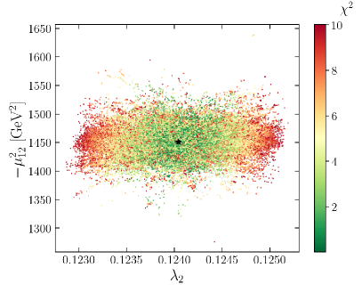
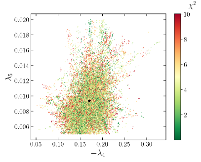
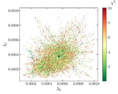
Figure 3: Some 2D projections of the most promising Higgs-potential parameter region of a stringy 2HDM, with $\chi^{2}\leq 10$ w.r.t. the observables in eq. (53). The black star corresponds to our best fit with $\chi^{2}=1.23\times 10^{-4}$.

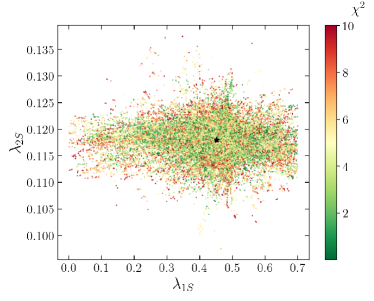
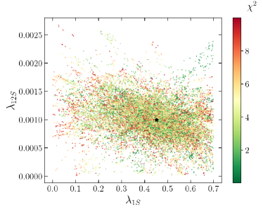
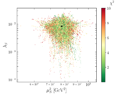
Figure 4: 2D projections of the viable Higgs-portal parameter region of our model with $\chi^{2}\leq 10$ compatibility with observations. For some parameters the validity region is much wider than for others. The best fit is given by the point highlighted with the black star.

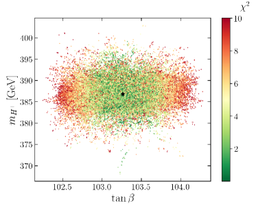
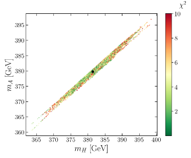
Figure 5: Predictions of a stringy 2HDM with Higgs portals on $\tan\beta$ and the masses of the heavier Higgs sector. We observe a quasi-linear dependence in the masses of the heavier (scalar and pseudoscalar) Higgs fields, which are constrained to lie between 370 and 400 GeV for an accuracy of $\chi^{2}\leq 10$. The best fit is highlighted by the black star.

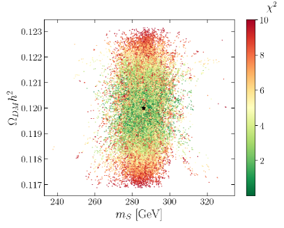
Figure 6: Predictions for the mass $m_{S}$ of the scalar DM candidate and its relic abundance. The preferred mass is $286.01\,$GeV and the best fit of $\Omega_{\mathrm{DM}}h^{2}$ coincides with the observed value $0.12$.

7 Conclusions

In order to arrive at a proof of concept of interesting DM phenomenology in non-SUSY orbifold compactifications of the heterotic string, we have shown that Higgs-portal scenarios arise naturally in this context and that they can readily accommodate observations on DM and Higgs physics.

We recall that the most common SM-like string models without leptoquarks and a minimum of vectorlike exotics exhibits six Higgs fields and some continuous gauge flavor symmetry. Even though the number of Higgses is large, the flavor symmetry reduces the degrees of freedom. We have inspected the structure of a sample model of this type. It displays promising Higgs-portal DM scenarios, i.e. scalar DM candidates coupling only to multi-Higgs sectors at leading order. This feature is quite general in this type of constructions. However, the complexity of the structure of Higgs vacua forces one to adopt very strong ad hoc constraints that weaken the predictivity of the model.

Hence, we have studied in more detail a simpler sample 2HDM arising from heterotic orbifolds. We find that the appearance of Higgs portals is generic in this kind of models too. The resulting effective field theory has the advantage that the Higgs vacuum is more tractable. Hence, we have used various numeric tools to scan the parameter space for phenomenologically viable regions, including 1-loop corrections. We have identified vast promising neighborhoods (with $\chi^{2}\leq 10$) endowed with i) stable Higgs vacua, ii) lightest Higgs mass and VEV compatible with experiments, and iii) freeze-out DM relic abundance consistent with observational data. Further, we have found that in those cases, as illustrated in figure 5, $\tan\beta\sim 100$, the heavier (scalar and pseudoscalar) Higgs fields have masses around 380 GeV, and the scalar DM candidate displays $m_{S}\sim 285$ GeV. We have identified a best fit to data of our stringy 2HDM with $\chi^{2}=1.23\times 10^{-4}$. Its details are given in table 3. All of these results can be considered predictions of models like ours, independently of whether they are motivated by top-down or bottom-up considerations.

There are various challenges to be addressed elsewhere in order to complete the study of this and similar models in the context of non-SUSY string compactifications. They include the phenomenology of the leptoquarks appearing in our 2HDM and other similar string models; their flavor structure and phenomenology, involving all gauge, traditional and modular flavor symmetries of the model (see e.g. [28, 98, 30, 99, 100, 31]); the possibility of Higgs portals with multiple DM candidates, including the likely existence of extra pseudoscalars; and the stringy computation of the couplings and their RGE running from the compactification scale. In particular, the appearance of a few leptoquarks and their (possibly negligible) couplings to the SM must be further studied as they may be relevant for extant questions in the SM [101] and even for richer DM scenarios [102].

Appendix A Spectrum of the stringy model with six Higgses

Table 4: Spectrum of massless fermions for the non-SUSY stringy model with six Higgs doublets introduced in section 4. The first column corresponds to the multiplicity of the fields. We show the quantum numbers with respect to the 4D gauge group, $\mathcal{G}_{\text{4D}}=\mathcal{G}_{\text{SM}}\times\mathcal{G}^{\prime}\times\mathrm{U}(1)^{\prime 8}$, where $\mathcal{G}_{\text{SM}}=\mathrm{SU}(3)_{c}\times\mathrm{SU}(2)_{L}\times\mathrm{U}(1)_{Y}$ and $\mathcal{G}^{\prime}=\mathrm{SU}(3)_{\mathrm{flavor}}\times\mathrm{SU}(2)\times\mathrm{SU}(2)$. The first $\mathrm{U}(1)^{\prime}$, associated with the charges $q_{1}$, is (pseudo-)anomalous. In the column labeled as $\mathrm{SU}(3)$ we list the $\mathrm{SU}(3)_{\mathrm{flavor}}$ representations.

#	$\mathcal{G}_{\text{SM}}$	$\mathrm{SU}(3)$	$\mathrm{SU}(2)$	$\mathrm{SU}(2)$	$q_{1}$	$q_{2}$	$q_{3}$	$q_{4}$	$q_{5}$	$q_{6}$	$q_{7}$	$q_{8}$	label
1	$(\boldsymbol{1},\boldsymbol{2})_{\nicefrac{{-1}}{{2}}}$	$\boldsymbol{1}$	$\boldsymbol{1}$	$\boldsymbol{1}$	-3	3	-27	-9	-9	9	-9	42	$\ell_{\mathrm{L},1}$
2	$(\boldsymbol{1},\boldsymbol{2})_{\nicefrac{{-1}}{{2}}}$	$\boldsymbol{1}$	$\boldsymbol{1}$	$\boldsymbol{1}$	2	3	1	25	-13	13	-13	32	$\ell_{\mathrm{L},2i}$
1	$(\boldsymbol{1},\boldsymbol{2})_{\nicefrac{{-1}}{{2}}}$	$\boldsymbol{1}$	$\boldsymbol{1}$	$\boldsymbol{1}$	0	-18	-6	-2	-2	2	-2	-48	$\ell_{\mathrm{L},3}$
1	$(\boldsymbol{1},\boldsymbol{2})_{\nicefrac{{-1}}{{2}}}$	$\boldsymbol{1}$	$\boldsymbol{1}$	$\boldsymbol{1}$	2	0	-56	6	6	-6	6	-28	$\ell_{\mathrm{L},4}$
1	$(\boldsymbol{1},\boldsymbol{2})_{\nicefrac{{1}}{{2}}}$	$\boldsymbol{1}$	$\boldsymbol{1}$	$\boldsymbol{1}$	0	18	6	2	2	-2	2	48	$\overline{\ell}^{\prime}_{\mathrm{L},1}$
1	$(\boldsymbol{1},\boldsymbol{2})_{\nicefrac{{1}}{{2}}}$	$\boldsymbol{1}$	$\boldsymbol{1}$	$\boldsymbol{1}$	0	0	0	-74	2	-2	2	48	$\overline{\ell}^{\prime}_{\mathrm{L},2}$
1	$(\boldsymbol{1},\boldsymbol{1})_{1}$	$\boldsymbol{3}$	$\boldsymbol{1}$	$\boldsymbol{1}$	1	-1	9	3	3	-3	3	-14	$\overline{e}_{\mathrm{L}}$
1	$(\boldsymbol{3},\boldsymbol{2})_{\nicefrac{{1}}{{6}}}$	$\boldsymbol{3}$	$\boldsymbol{1}$	$\boldsymbol{1}$	1	-1	9	3	3	-3	3	-14	$q_{\mathrm{L}}$
1	$(\boldsymbol{\overline{3}},\boldsymbol{1})_{\nicefrac{{-2}}{{3}}}$	$\boldsymbol{3}$	$\boldsymbol{1}$	$\boldsymbol{1}$	1	-1	9	3	3	-3	3	-14	$\overline{u}_{\mathrm{L}}$
1	$(\boldsymbol{\overline{3}},\boldsymbol{1})_{\nicefrac{{1}}{{3}}}$	$\boldsymbol{1}$	$\boldsymbol{1}$	$\boldsymbol{1}$	-3	3	-27	-9	-9	9	-9	42	$\overline{d}_{\mathrm{L},1}$
4	$(\boldsymbol{\overline{3}},\boldsymbol{1})_{\nicefrac{{1}}{{3}}}$	$\boldsymbol{1}$	$\boldsymbol{1}$	$\boldsymbol{1}$	2	3	1	25	-13	13	-13	32	$\overline{d}_{\mathrm{L},2i}$
1	$(\boldsymbol{\overline{3}},\boldsymbol{1})_{\nicefrac{{1}}{{3}}}$	$\boldsymbol{1}$	$\boldsymbol{1}$	$\boldsymbol{1}$	2	0	-56	6	6	-6	6	-28	$\overline{d}_{\mathrm{L},3}$
1	$(\boldsymbol{\overline{3}},\boldsymbol{1})_{\nicefrac{{1}}{{3}}}$	$\boldsymbol{1}$	$\boldsymbol{1}$	$\boldsymbol{1}$	0	0	0	0	76	2	-2	-48	$\overline{d}_{\mathrm{L},4}$
2	$(\boldsymbol{3},\boldsymbol{1})_{\nicefrac{{-1}}{{3}}}$	$\boldsymbol{1}$	$\boldsymbol{1}$	$\boldsymbol{1}$	-2	-3	-1	-25	13	-13	13	-32	$d^{\prime}_{\mathrm{L},1i}$
1	$(\boldsymbol{3},\boldsymbol{1})_{\nicefrac{{-1}}{{3}}}$	$\boldsymbol{1}$	$\boldsymbol{1}$	$\boldsymbol{1}$	0	0	0	-74	2	-2	2	48	$d^{\prime}_{\mathrm{L},2}$
1	$(\boldsymbol{3},\boldsymbol{1})_{\nicefrac{{-1}}{{3}}}$	$\boldsymbol{1}$	$\boldsymbol{1}$	$\boldsymbol{1}$	0	0	0	0	-76	-2	2	48	$d^{\prime}_{\mathrm{L},3}$
1	$(\boldsymbol{1},\boldsymbol{1})_{0}$	$\boldsymbol{1}$	$\boldsymbol{1}$	$\boldsymbol{1}$	-1	-9	25	-41	35	-35	-47	-10	$\nu_{\mathrm{R},1}$
1	$(\boldsymbol{1},\boldsymbol{1})_{0}$	$\boldsymbol{1}$	$\boldsymbol{2}$	$\boldsymbol{2}$	1	9	-25	41	-35	-4	4	10	$\nu_{\mathrm{R},2}$
1	$(\boldsymbol{1},\boldsymbol{1})_{0}$	$\boldsymbol{1}$	$\boldsymbol{1}$	$\boldsymbol{1}$	-1	-9	25	-41	35	43	39	-10	$\nu_{\mathrm{R},3}$
1	$(\boldsymbol{1},\boldsymbol{1})_{0}$	$\boldsymbol{1}$	$\boldsymbol{1}$	$\boldsymbol{1}$	1	-3	27	9	9	-9	9	130	$\nu_{\mathrm{R},4}$
1	$(\boldsymbol{1},\boldsymbol{1})_{0}$	$\boldsymbol{1}$	$\boldsymbol{1}$	$\boldsymbol{1}$	1	-9	-31	39	39	39	-39	10	$\nu_{\mathrm{R},5}$
1	$(\boldsymbol{1},\boldsymbol{1})_{0}$	$\boldsymbol{1}$	$\boldsymbol{1}$	$\boldsymbol{1}$	1	9	31	-39	-39	39	-39	10	$\nu_{\mathrm{R},6}$
1	$(\boldsymbol{1},\boldsymbol{1})_{0}$	$\boldsymbol{1}$	$\boldsymbol{2}$	$\boldsymbol{2}$	1	-9	-31	-35	-35	-4	4	10	$\nu_{\mathrm{R},7}$
1	$(\boldsymbol{1},\boldsymbol{1})_{0}$	$\boldsymbol{1}$	$\boldsymbol{1}$	$\boldsymbol{1}$	-1	-9	25	33	-43	-35	-47	-10	$\nu_{\mathrm{R},8}$
1	$(\boldsymbol{1},\boldsymbol{1})_{0}$	$\boldsymbol{1}$	$\boldsymbol{1}$	$\boldsymbol{1}$	1	9	-25	-33	43	-43	-39	10	$\nu_{\mathrm{R},9}$
1	$(\boldsymbol{1},\boldsymbol{1})_{0}$	$\boldsymbol{1}$	$\boldsymbol{2}$	$\boldsymbol{2}$	-1	9	31	35	35	4	-4	-10	$\nu_{\mathrm{R},10}$
1	$(\boldsymbol{1},\boldsymbol{1})_{0}$	$\boldsymbol{1}$	$\boldsymbol{1}$	$\boldsymbol{1}$	-1	-9	25	33	-43	43	39	-10	$\nu_{\mathrm{R},11}$
1	$(\boldsymbol{1},\boldsymbol{1})_{0}$	$\boldsymbol{1}$	$\boldsymbol{1}$	$\boldsymbol{1}$	1	9	-25	-33	43	35	47	10	$\nu_{\mathrm{R},12}$
2	$(\boldsymbol{1},\boldsymbol{1})_{0}$	$\boldsymbol{\overline{3}}$	$\boldsymbol{1}$	$\boldsymbol{1}$	0	-5	17	-19	19	-19	19	-60	$\nu^{\prime}_{\mathrm{R},13,i}$
2	$(\boldsymbol{1},\boldsymbol{1})_{0}$	$\boldsymbol{1}$	$\boldsymbol{1}$	$\boldsymbol{1}$	5/2	0	14	-20	-39	-39	-2	-5	$\nu_{\mathrm{R},14,i}$
2	$(\boldsymbol{1},\boldsymbol{1})_{0}$	$\boldsymbol{1}$	$\boldsymbol{1}$	$\boldsymbol{1}$	3/2	0	14	54	35	-35	-6	-15	$\nu_{\mathrm{R},15,i}$
2	$(\boldsymbol{1},\boldsymbol{1})_{0}$	$\boldsymbol{1}$	$\boldsymbol{2}$	$\boldsymbol{1}$	5/2	0	14	-20	37	2	-2	-5	$\nu_{\mathrm{R},16,i}$
2	$(\boldsymbol{1},\boldsymbol{1})_{0}$	$\boldsymbol{1}$	$\boldsymbol{1}$	$\boldsymbol{2}$	5/2	0	14	-20	37	2	-2	-5	$\nu_{\mathrm{R},17,i}$
2	$(\boldsymbol{1},\boldsymbol{1})_{0}$	$\boldsymbol{1}$	$\boldsymbol{1}$	$\boldsymbol{1}$	5/2	0	14	-20	-39	0	41	-5	$\nu_{\mathrm{R},18,i}$
2	$(\boldsymbol{1},\boldsymbol{1})_{0}$	$\boldsymbol{1}$	$\boldsymbol{1}$	$\boldsymbol{1}$	3/2	0	14	54	35	4	37	-15	$\nu_{\mathrm{R},19,i}$
2	$(\boldsymbol{1},\boldsymbol{1})_{0}$	$\boldsymbol{1}$	$\boldsymbol{1}$	$\boldsymbol{1}$	3/2	6	16	30	11	-11	-30	-75	$\nu_{\mathrm{R},20,i}$
2	$(\boldsymbol{1},\boldsymbol{1})_{0}$	$\boldsymbol{\overline{3}}$	$\boldsymbol{1}$	$\boldsymbol{1}$	1/2	-2	-24	-8	-27	27	14	35	$\nu^{\prime}_{\mathrm{R},21,i}$
2	$(\boldsymbol{1},\boldsymbol{1})_{0}$	$\boldsymbol{1}$	$\boldsymbol{1}$	$\boldsymbol{1}$	3/2	6	16	30	11	28	13	-75	$\nu_{\mathrm{R},22,i}$
2	$(\boldsymbol{1},\boldsymbol{1})_{0}$	$\boldsymbol{\overline{3}}$	$\boldsymbol{1}$	$\boldsymbol{1}$	1/2	-2	-24	-8	-27	-12	-29	35	$\nu^{\prime}_{\mathrm{R},23,i}$
1	$(\boldsymbol{1},\boldsymbol{1})_{0}$	$\boldsymbol{\overline{3}}$	$\boldsymbol{1}$	$\boldsymbol{1}$	0	-2	74	0	0	0	0	0	$\nu^{\prime}_{\mathrm{R},24}$
1	$(\boldsymbol{1},\boldsymbol{1})_{0}$	$\boldsymbol{3}$	$\boldsymbol{1}$	$\boldsymbol{1}$	-2	2	-18	68	-8	8	-8	-20	$\nu^{\prime\prime}_{\mathrm{R},25}$
1	$(\boldsymbol{1},\boldsymbol{1})_{0}$	$\boldsymbol{\overline{3}}$	$\boldsymbol{1}$	$\boldsymbol{1}$	2	16	24	8	8	-8	8	20	$\nu^{\prime}_{\mathrm{R},26}$
1	$(\boldsymbol{1},\boldsymbol{1})_{0}$	$\boldsymbol{3}$	$\boldsymbol{1}$	$\boldsymbol{1}$	-2	-16	-24	-8	-8	8	-8	-20	$\nu^{\prime\prime}_{\mathrm{R},27}$
4	$(\boldsymbol{1},\boldsymbol{1})_{0}$	$\boldsymbol{1}$	$\boldsymbol{1}$	$\boldsymbol{1}$	1	6	-26	-58	-20	20	-20	-50	$\nu_{\mathrm{R},28,i}$
2	$(\boldsymbol{1},\boldsymbol{1})_{0}$	$\boldsymbol{1}$	$\boldsymbol{1}$	$\boldsymbol{1}$	-1	-6	26	58	20	-20	20	50	$\nu_{\mathrm{R},29,i}$
2	$(\boldsymbol{1},\boldsymbol{1})_{0}$	$\boldsymbol{1}$	$\boldsymbol{1}$	$\boldsymbol{1}$	1	-6	-30	-10	28	-28	28	70	$\nu_{\mathrm{R},30,i}$
2	$(\boldsymbol{1},\boldsymbol{1})_{0}$	$\boldsymbol{1}$	$\boldsymbol{1}$	$\boldsymbol{1}$	3/2	-3	13	29	-28	-11	-30	-75	$\nu_{\mathrm{R},31,i}$
2	$(\boldsymbol{1},\boldsymbol{1})_{0}$	$\boldsymbol{\overline{3}}$	$\boldsymbol{1}$	$\boldsymbol{1}$	1/2	7	-21	-7	12	27	14	35	$\nu^{\prime}_{\mathrm{R},32,i}$
2	$(\boldsymbol{1},\boldsymbol{1})_{0}$	$\boldsymbol{1}$	$\boldsymbol{1}$	$\boldsymbol{1}$	3/2	-3	13	29	-28	28	13	-75	$\nu_{\mathrm{R},33,i}$
2	$(\boldsymbol{1},\boldsymbol{1})_{0}$	$\boldsymbol{\overline{3}}$	$\boldsymbol{1}$	$\boldsymbol{1}$	1/2	7	-21	-7	12	-12	-29	35	$\nu^{\prime}_{\mathrm{R},34,i}$
2	$(\boldsymbol{1},\boldsymbol{1})_{0}$	$\boldsymbol{1}$	$\boldsymbol{1}$	$\boldsymbol{1}$	3/2	-9	11	53	-4	-35	-6	-15	$\nu_{\mathrm{R},35,i}$
2	$(\boldsymbol{1},\boldsymbol{1})_{0}$	$\boldsymbol{1}$	$\boldsymbol{2}$	$\boldsymbol{1}$	5/2	-9	11	-21	-2	2	-2	-5	$\nu_{\mathrm{R},36,i}$
2	$(\boldsymbol{1},\boldsymbol{1})_{0}$	$\boldsymbol{1}$	$\boldsymbol{1}$	$\boldsymbol{1}$	5/2	9	17	-19	0	-39	-2	-5	$\nu_{\mathrm{R},37,i}$
2	$(\boldsymbol{1},\boldsymbol{1})_{0}$	$\boldsymbol{1}$	$\boldsymbol{1}$	$\boldsymbol{2}$	5/2	-9	11	-21	-2	2	-2	-5	$\nu_{\mathrm{R},38,i}$
2	$(\boldsymbol{1},\boldsymbol{1})_{0}$	$\boldsymbol{1}$	$\boldsymbol{1}$	$\boldsymbol{1}$	3/2	-9	11	53	-4	4	37	-15	$\nu_{\mathrm{R},39,i}$
2	$(\boldsymbol{1},\boldsymbol{1})_{0}$	$\boldsymbol{1}$	$\boldsymbol{1}$	$\boldsymbol{1}$	5/2	9	17	-19	0	0	41	-5	$\nu_{\mathrm{R},40,i}$

Table 5: Stringy spectrum of massless complex scalars for a model with six Higgses. Note that our DM candidate $S$ has the same charges as $s_{10}$. We follow the same notation as in table LABEL:tab:complete4902f.

#	$\mathcal{G}_{\text{SM}}$	$\mathrm{SU}(3)$	$\mathrm{SU}(2)$	$\mathrm{SU}(2)$	$q_{1}$	$q_{2}$	$q_{3}$	$q_{4}$	$q_{5}$	$q_{6}$	$q_{7}$	$q_{8}$	label
2	$(\boldsymbol{1},\boldsymbol{2})_{\nicefrac{{1}}{{2}}}$	$\boldsymbol{3}$	$\boldsymbol{1}$	$\boldsymbol{1}$	-2	2	-18	-6	-6	6	-6	28	$\phi_{i}$
1	$(\boldsymbol{1},\boldsymbol{1})_{0}$	$\boldsymbol{1}$	$\boldsymbol{1}$	$\boldsymbol{1}$	3/2	9	45	15	-4	-35	-6	-15	$S$
1	$(\boldsymbol{1},\boldsymbol{1})_{0}$	$\boldsymbol{1}$	$\boldsymbol{1}$	$\boldsymbol{1}$	0	-18	-6	-76	0	0	0	0	$s_{1}$
1	$(\boldsymbol{1},\boldsymbol{1})_{0}$	$\boldsymbol{1}$	$\boldsymbol{1}$	$\boldsymbol{1}$	0	0	0	74	-78	0	0	0	$s_{2}$
1	$(\boldsymbol{1},\boldsymbol{1})_{0}$	$\boldsymbol{1}$	$\boldsymbol{1}$	$\boldsymbol{1}$	-2	0	56	-6	70	8	-8	-20	$s_{3}$
1	$(\boldsymbol{1},\boldsymbol{1})_{0}$	$\boldsymbol{1}$	$\boldsymbol{1}$	$\boldsymbol{1}$	2	18	-50	8	8	-8	8	20	$s_{4}$
2	$(\boldsymbol{1},\boldsymbol{1})_{0}$	$\boldsymbol{1}$	$\boldsymbol{1}$	$\boldsymbol{2}$	3/2	-9	39	13	-6	6	-6	-15	$s_{5}$
2	$(\boldsymbol{1},\boldsymbol{1})_{0}$	$\boldsymbol{1}$	$\boldsymbol{1}$	$\boldsymbol{1}$	5/2	-9	-17	19	0	0	41	-5	$s_{6}$
2	$(\boldsymbol{1},\boldsymbol{1})_{0}$	$\boldsymbol{1}$	$\boldsymbol{1}$	$\boldsymbol{1}$	3/2	9	45	15	-4	4	37	-15	$s_{7}$
2	$(\boldsymbol{1},\boldsymbol{1})_{0}$	$\boldsymbol{1}$	$\boldsymbol{1}$	$\boldsymbol{1}$	5/2	-9	-17	19	0	-39	-2	-5	$s_{8}$
2	$(\boldsymbol{1},\boldsymbol{1})_{0}$	$\boldsymbol{1}$	$\boldsymbol{2}$	$\boldsymbol{1}$	3/2	-9	39	13	-6	6	-6	-15	$s_{9}$
1	$(\boldsymbol{1},\boldsymbol{1})_{0}$	$\boldsymbol{1}$	$\boldsymbol{1}$	$\boldsymbol{1}$	3/2	9	45	15	-4	-35	-6	-15	$s_{10}$
2	$(\boldsymbol{1},\boldsymbol{1})_{0}$	$\boldsymbol{1}$	$\boldsymbol{1}$	$\boldsymbol{1}$	5/2	-3	-15	-5	-24	24	17	-65	$s_{11}$
2	$(\boldsymbol{1},\boldsymbol{1})_{0}$	$\boldsymbol{3}$	$\boldsymbol{1}$	$\boldsymbol{1}$	1/2	-7	-7	-27	-8	8	33	-25	$s^{\prime}_{12}$
2	$(\boldsymbol{1},\boldsymbol{1})_{0}$	$\boldsymbol{1}$	$\boldsymbol{1}$	$\boldsymbol{1}$	5/2	-3	-15	-5	-24	-15	-26	-65	$s_{13}$
2	$(\boldsymbol{1},\boldsymbol{1})_{0}$	$\boldsymbol{3}$	$\boldsymbol{1}$	$\boldsymbol{1}$	1/2	-7	-7	-27	-8	-31	-10	-25	$s^{\prime}_{14}$
6	$(\boldsymbol{1},\boldsymbol{1})_{0}$	$\boldsymbol{1}$	$\boldsymbol{1}$	$\boldsymbol{1}$	-2	-3	-1	49	11	-11	11	-80	$s_{15}$
2	$(\boldsymbol{1},\boldsymbol{1})_{0}$	$\boldsymbol{1}$	$\boldsymbol{1}$	$\boldsymbol{1}$	0	3	57	19	-19	19	-19	60	$s_{16}$
2	$(\boldsymbol{1},\boldsymbol{1})_{0}$	$\boldsymbol{3}$	$\boldsymbol{1}$	$\boldsymbol{1}$	1/2	2	-4	-26	31	-31	-10	-25	$s^{\prime}_{17}$
2	$(\boldsymbol{1},\boldsymbol{1})_{0}$	$\boldsymbol{1}$	$\boldsymbol{1}$	$\boldsymbol{1}$	-5/2	-6	12	4	-15	15	26	65	$s_{18}$
2	$(\boldsymbol{1},\boldsymbol{1})_{0}$	$\boldsymbol{3}$	$\boldsymbol{1}$	$\boldsymbol{1}$	1/2	2	-4	-26	31	8	33	-25	$s^{\prime}_{19}$
2	$(\boldsymbol{1},\boldsymbol{1})_{0}$	$\boldsymbol{1}$	$\boldsymbol{1}$	$\boldsymbol{1}$	-5/2	-6	12	4	-15	-24	-17	65	$s_{20}$
2	$(\boldsymbol{1},\boldsymbol{1})_{0}$	$\boldsymbol{1}$	$\boldsymbol{2}$	$\boldsymbol{1}$	-3/2	0	-42	-14	-33	-6	6	15	$s_{21}$
2	$(\boldsymbol{1},\boldsymbol{1})_{0}$	$\boldsymbol{1}$	$\boldsymbol{1}$	$\boldsymbol{1}$	-3/2	0	-42	-14	43	35	6	15	$s_{22}$
2	$(\boldsymbol{1},\boldsymbol{1})_{0}$	$\boldsymbol{1}$	$\boldsymbol{1}$	$\boldsymbol{1}$	-5/2	0	14	-20	-39	39	2	5	$s_{23}$
2	$(\boldsymbol{1},\boldsymbol{1})_{0}$	$\boldsymbol{1}$	$\boldsymbol{1}$	$\boldsymbol{2}$	-3/2	0	-42	-14	-33	-6	6	15	$s_{24}$
2	$(\boldsymbol{1},\boldsymbol{1})_{0}$	$\boldsymbol{1}$	$\boldsymbol{1}$	$\boldsymbol{1}$	-3/2	0	-42	-14	43	-4	-37	15	$s_{25}$
2	$(\boldsymbol{1},\boldsymbol{1})_{0}$	$\boldsymbol{1}$	$\boldsymbol{1}$	$\boldsymbol{1}$	-5/2	0	14	-20	-39	0	-41	5	$s_{26}$

A.1 Hypercharge generator

The generator $Q_{Y}$ of $\mathrm{U}(1)_{Y}$ in $\mathcal{G}_{\text{SM}}\subset\mathcal{G}_{\text{4D}}$ is given by (cf. e.g. [68, 69, 103])

$$Q_{Y}~{}=~{}\sum_{I=1}^{16}t^{I}_{Y}H_{I}\,,$$ (56)

in terms of the $\mathrm{SO}(16)$$\times$$\mathrm{SO}(16)$ Cartan generators $H^{I}$. Frequently, the 16D vector $t_{Y}$ is also called $\mathrm{U}(1)_{Y}$ generator. For our six-Higgs model, we identify

$$t_{Y}=(\tfrac{1}{3},0,0,0,-\tfrac{1}{3},-\tfrac{1}{2},-\tfrac{1}{2},\tfrac{1}{3},0,0,0,0,0,0,0,0)$$ (57)

with normalization $t_{Y}\cdot t_{Y}=\nicefrac{{5}}{{6}}$. Note that this normalization makes the hypercharge compatible with $\mathrm{SU}(5)$ unification, as [73, eq. (3)] $\sin^{2}\theta_{W}=1/(1+k_{1})=\nicefrac{{3}}{{8}}$ at the string scale, since the hypercharge level is given by [73, below eq. (4)] $k_{1}=2\,t_{Y}\cdot t_{Y}=\nicefrac{{5}}{{3}}$. The hypercharge $q_{Y}$ of effective fields with gauge momenta $p\,\in\,\mathrm{SO}(16)\times\mathrm{SO}(16)$ is given by $q_{Y}=t_{Y}\cdot p$.

Appendix B Fermionic mass matrices of the six-Higgs-doublet model

Let us provide some details on the computation of the fermionic mass eigenstates for quarks and leptons prior to electroweak symmetry breakdown, due to the existence of exotics in the model. To simplify the notation, we use $\braket{s_{i}}\to s_{i}$ for the singlet VEVs. Given the mass matrix for the leptons in eq. (6) and the chosen VEV configuration in eq. (8). The squared matrix is given by

$$M_{\ell}^{\intercal}\,M_{\ell}=\begin{pmatrix}0&0&0&0&0\\ 0&0&0&0&0\\ 0&0&0&0&0\\ 0&0&0&c_{1}^{2}+c_{5}^{2}s_{1}^{2}&c_{1}c_{2}s_{4}\\ 0&0&0&c_{1}c_{2}s_{4}&c_{2}^{2}s_{4}^{2}\end{pmatrix}\,.$$ (58)

The corresponding unnormalized physical lepton states are given in terms of the original stringy states by

$$\begin{pmatrix}\ell_{\mathrm{L},1}\\ \ell_{\mathrm{L},2}\\ \ell_{\mathrm{L},3}\\ \ell_{\mathrm{L},4}\\ \ell_{\mathrm{L},5}\\ \end{pmatrix}_{\mathrm{phys}}:=~{}\begin{pmatrix}1&0&0&0&0\\ 0&1&0&0&0\\ 0&0&1&0&0\\ 0&0&0&w_{-}&1\\ 0&0&0&w_{+}&1\end{pmatrix}\begin{pmatrix}\ell_{\mathrm{L},1}\\ \ell_{\mathrm{L},21}\\ \ell_{\mathrm{L},22}\\ \ell_{\mathrm{L},3}\\ \ell_{\mathrm{L},4}\\ \end{pmatrix}\,,$$ (59)

where

$$w_{\pm}:=\frac{c_{1}^{2}+c_{5}^{2}s_{1}^{2}-c_{2}^{2}s_{4}^{2}\pm\sqrt{(c_{1}^{2}+c_{5}^{2}s_{1}^{2})^{2}+2c_{2}^{2}(c_{1}-c_{5}s_{1})(c_{1}+c_{5}s_{1})s_{4}^{2}+c_{2}^{4}s_{4}^{4}}}{2c_{1}c_{2}s_{4}}\,.$$ (60)

We must perform an analogous procedure for down-quark singlets. According to table 1, in our model there are seven left-handed down-quark singlets, $\overline{d}:=\left(\overline{d}_{\mathrm{L},1},\,\overline{d}_{\mathrm{L},21},\,\overline{d}_{\mathrm{L},22},\,\overline{d}_{\mathrm{L},23},\,\overline{d}_{\mathrm{L},24},\,\overline{d}_{\mathrm{L},3},\,\overline{d}_{\mathrm{L},4}\right)$, and four left-handed conjugate states, $d^{\prime}:=(d^{\prime}_{\mathrm{L},11},\,d^{\prime}_{\mathrm{L},12},\,d^{\prime}_{\mathrm{L},2},\,d^{\prime}_{\mathrm{L},3})^{\intercal}$. Thus, we find the low-energy physical states by building the mass eigenstates. Using the charges of these fields in table LABEL:tab:complete4902f, we can find the resulting admissible couplings that lead to

$$\overline{d}\,M_{d}\,d^{\prime}~{}\subset~{}\mathcal{L}\,.$$ (61)

At leading order, the down-quark mass matrix is given by

$$M_{d}~{}=\begin{pmatrix}0&0&0&0\\ c^{d}_{1}&c^{d}_{2}&s_{15}&0\\ c^{d}_{3}&c^{d}_{4}&s_{15}&0\\ c^{d}_{5}&c^{d}_{6}&s_{15}&0\\ c^{d}_{7}&c^{d}_{8}&s_{15}&0\\ c^{d}_{9}s_{16}&c^{d}_{10}s_{16}&0&c^{d}_{11}s_{3}\\ 0&0&c^{d}_{12}s_{2}&c^{d}_{13}\end{pmatrix}\,.$$ (62)

As in the leptonic case, the coefficients $c^{d}_{i}$ are some coupling constants that are assumed to be real and order unity. In addition, to be consistent with the leptonic case, we take $s_{15}=0$ and this is why we omit the coupling constants of $s_{15}\overline{d}_{\mathrm{L},2i}d_{\mathrm{L},1j}$ in eq. (62). It is easy to verify that the down-quark mass matrix has full rank 4. Hence, in the notation of table LABEL:tab:complete4902f, the physical (massless) down-quark singlets are $\overline{d}_{\mathrm{L},1}$ and the combinations

$$\overline{d}_{\mathrm{L},24}-\frac{c^{d}_{2}c^{d}_{7}-c^{d}_{1}c^{d}_{8}}{c^{d}_{2}c^{d}_{3}-c^{d}_{1}c^{d}_{4}}\overline{d}_{\mathrm{L},22}-\frac{c^{d}_{4}c^{d}_{7}-c^{d}_{3}c^{d}_{8}}{c^{d}_{1}c^{d}_{4}-c^{d}_{2}c^{d}_{3}}\overline{d}_{\mathrm{L},21}\,,\quad\overline{d}_{\mathrm{L},23}-\frac{c^{d}_{2}c^{d}_{5}-c^{d}_{1}c^{d}_{6}}{c^{d}_{2}c^{d}_{3}-c^{d}_{1}c^{d}_{4}}\overline{d}_{\mathrm{L},22}-\frac{c^{d}_{4}c^{d}_{5}-c^{d}_{3}c^{d}_{6}}{c^{d}_{1}c^{d}_{4}-c^{d}_{2}c^{d}_{3}}\overline{d}_{\mathrm{L},21}.$$ (63)

Now, we relabel the massless eigenstates as

$$\begin{split}&\overline{d}_{\mathrm{L},1}\to\overline{d}_{\mathrm{L},1}\\ &\overline{d}_{\mathrm{L},24}-\frac{c^{d}_{2}c^{d}_{7}-c^{d}_{1}c^{d}_{8}}{c^{d}_{2}c^{d}_{3}-c^{d}_{1}c^{d}_{4}}\overline{d}_{\mathrm{L},22}-\frac{c^{d}_{4}c^{d}_{7}-c^{d}_{3}c^{d}_{8}}{c^{d}_{1}c^{d}_{4}-c^{d}_{2}c^{d}_{3}}\overline{d}_{\mathrm{L},21}\to\overline{d}_{\mathrm{L},2}\\ &\overline{d}_{\mathrm{L},23}-\frac{c^{d}_{2}c^{d}_{5}-c^{d}_{1}c^{d}_{6}}{c^{d}_{2}c^{d}_{3}-c^{d}_{1}c^{d}_{4}}\overline{d}_{\mathrm{L},22}-\frac{c^{d}_{4}c^{d}_{5}-c^{d}_{3}c^{d}_{6}}{c^{d}_{1}c^{d}_{4}-c^{d}_{2}c^{d}_{3}}\overline{d}_{\mathrm{L},21}\to\overline{d}_{\mathrm{L},3}\,.\end{split}$$ (64)

Appendix C Coefficients of the six-Higgs-doublet sector

The quadratic terms of the neutral components in the Higgs-sector potential (16) are

$$\begin{split}V_{\phi}(\sigma_{1I},\sigma_{2I})~{}\supset~{}&\theta_{IJ}\sigma_{1I}\sigma_{2J}^{*}+\chi_{IJ}\sigma_{1I}\sigma_{2J}+\kappa_{1,IJ}\sigma_{1I}\sigma_{1J}+\kappa_{2,IJ}\sigma_{2I}\sigma_{2J}\\ &+\omega_{1,IJ}\sigma_{1I}\sigma_{1J}^{*}+\left(\xi\delta_{IJ}+\omega_{2,IJ}\right)\sigma_{2I}\sigma_{2J}^{*}+\text{c.c.}\,,\end{split}$$ (65)

where $\delta_{IJ}$ is the usual Kronecker delta and

$$\begin{split}\theta_{IJ}&:=\lambda_{6}v_{1I}v_{1J}\,,\qquad\ \ \chi_{IJ}:=\lambda_{6}v_{1I}v_{1J}\,,\qquad\ \ \kappa_{1,IJ}:=\lambda_{1}v_{1I}v_{1J}\,,\\ \kappa_{2,IJ}&:=\lambda_{5}v_{1I}v_{1J}\,,\qquad\omega_{1,IJ}:=2\lambda_{1}v_{1I}v_{1J}\,,\qquad\omega_{2,IJ}:=\frac{1}{2}\lambda_{4}v_{1I}v_{1J}\,.\end{split}$$ (66)

The entries of the mass matrix (23), which follow from the potential (65) in the limit of $\epsilon^{2}\sim 0$, are given by

$$\begin{split}\Omega_{1}&:=\frac{1}{2}\omega_{1,11}+\kappa_{1,11}\,,\qquad\Omega_{2}:=\frac{1}{2}\omega_{2,11}+\kappa_{2,11}\,,\\ \xi&:=\mu_{22}^{2}+\frac{1}{2}\lambda_{3}v_{11}^{2}\qquad\text{and}\qquad P:=\theta_{11}+\chi_{11}\,.\end{split}$$ (67)

Here we assume the hierarchy $v_{11}\gg v_{12}\gg v_{13}$ via the parameter $\epsilon$, such that $\epsilon=v_{12}/v_{11}=v_{13}/v_{12}$, with $\epsilon^{2}\sim 0$.

Appendix D Spectrum for the stringy 2HDM

Table 6: Spectrum of massless fermions in a stringy 2HDM. The first column corresponds to the multiplicity of the fields. The 4D gauge group is $\mathcal{G}_{\text{4D}}=\mathcal{G}_{\text{SM}}\times\mathcal{G}^{\prime}\times\mathrm{U}(1)^{\prime 8}$, where $\mathcal{G}_{\text{SM}}=\mathrm{SU}(3)_{c}\times\mathrm{SU}(2)_{L}\times\mathrm{U}(1)_{Y}$ and $\mathcal{G}^{\prime}=\mathrm{SU}(2)_{\mathrm{flavor}}\times\mathrm{SU}(3)\times\mathrm{SU}(2)$. The first $\mathrm{U}(1)^{\prime}$, associated with the charges $q_{1}$ is (pseudo-)anomalous. The first column with the label $\mathrm{SU}(2)$ displays the representations under $\mathrm{SU}(2)_{\mathrm{flavor}}$.

#	$\mathcal{G}_{\text{SM}}$	$\mathrm{SU}(2)$	$\mathrm{SU}(3)$	$\mathrm{SU}(2)$	$q_{1}$	$q_{2}$	$q_{3}$	$q_{4}$	$q_{5}$	$q_{6}$	$q_{7}$	$q_{8}$	label
1	$(\boldsymbol{1},\boldsymbol{2})_{\nicefrac{{-1}}{{2}}}$	$\boldsymbol{1}$	$\boldsymbol{1}$	$\boldsymbol{1}$	-3	0	-3	-9	9	-9	-27	6	$\ell_{\mathrm{L},3}$
2	$(\boldsymbol{1},\boldsymbol{2})_{\nicefrac{{-1}}{{2}}}$	$\boldsymbol{1}$	$\boldsymbol{1}$	$\boldsymbol{1}$	2	0	-3	-9	9	-9	-27	6	$\ell_{\mathrm{L},i}$
1	$(\boldsymbol{1},\boldsymbol{1})_{1}$	$\boldsymbol{2}$	$\boldsymbol{1}$	$\boldsymbol{1}$	1	1	1	3	-3	3	9	-2	$\overline{e}_{\mathrm{L}}$
1	$(\boldsymbol{1},\boldsymbol{1})_{1}$	$\boldsymbol{1}$	$\boldsymbol{1}$	$\boldsymbol{1}$	1	-2	1	3	-3	3	9	-2	$\overline{e}_{\mathrm{L},3}$
1	$(\boldsymbol{3},\boldsymbol{2})_{\nicefrac{{1}}{{6}}}$	$\boldsymbol{2}$	$\boldsymbol{1}$	$\boldsymbol{1}$	1	1	1	3	-3	3	9	-2	$q_{\mathrm{L}}$
1	$(\boldsymbol{3},\boldsymbol{2})_{\nicefrac{{1}}{{6}}}$	$\boldsymbol{1}$	$\boldsymbol{1}$	$\boldsymbol{1}$	1	-2	1	3	-3	3	9	-2	$q_{\mathrm{L},3}$
1	$(\boldsymbol{\overline{3}},\boldsymbol{1})_{\nicefrac{{-2}}{{3}}}$	$\boldsymbol{2}$	$\boldsymbol{1}$	$\boldsymbol{1}$	1	1	1	3	-3	3	9	-2	$\overline{u}_{\mathrm{L}}$
1	$(\boldsymbol{\overline{3}},\boldsymbol{1})_{\nicefrac{{-2}}{{3}}}$	$\boldsymbol{1}$	$\boldsymbol{1}$	$\boldsymbol{1}$	1	-2	1	3	-3	3	9	-2	$\overline{u}_{\mathrm{L},3}$
1	$(\boldsymbol{\overline{3}},\boldsymbol{1})_{\nicefrac{{1}}{{3}}}$	$\boldsymbol{1}$	$\boldsymbol{1}$	$\boldsymbol{1}$	-3	0	-3	-9	9	-9	-27	6	$\overline{d}_{\mathrm{L},3}$
4	$(\boldsymbol{\overline{3}},\boldsymbol{1})_{\nicefrac{{1}}{{3}}}$	$\boldsymbol{1}$	$\boldsymbol{1}$	$\boldsymbol{1}$	2	0	-3	-9	9	-9	-27	6	$\overline{d}_{\mathrm{L},1i}$
2	$(\boldsymbol{3},\boldsymbol{1})_{\nicefrac{{-1}}{{3}}}$	$\boldsymbol{1}$	$\boldsymbol{1}$	$\boldsymbol{1}$	-2	0	3	9	-9	9	27	-6	$d^{\prime}_{\mathrm{L},1i}$
1	$(\boldsymbol{1},\boldsymbol{1})_{0}$	$\boldsymbol{1}$	$\boldsymbol{\overline{3}}$	$\boldsymbol{2}$	1	0	-9	-27	27	3	-23	2	$\nu_{\mathrm{R},1}$
1	$(\boldsymbol{1},\boldsymbol{1})_{0}$	$\boldsymbol{1}$	$\boldsymbol{1}$	$\boldsymbol{1}$	1	0	-9	29	-29	-31	-93	2	$\nu_{\mathrm{R},2}$
1	$(\boldsymbol{1},\boldsymbol{1})_{0}$	$\boldsymbol{1}$	$\boldsymbol{\overline{3}}$	$\boldsymbol{1}$	-1	0	9	27	-27	27	-47	-2	$\nu_{\mathrm{R},3}$
1	$(\boldsymbol{1},\boldsymbol{1})_{0}$	$\boldsymbol{1}$	$\boldsymbol{1}$	$\boldsymbol{1}$	-1	0	9	27	-27	-33	93	-2	$\nu_{\mathrm{R},4}$
1	$(\boldsymbol{1},\boldsymbol{1})_{0}$	$\boldsymbol{1}$	$\boldsymbol{1}$	$\boldsymbol{1}$	1	0	3	9	-9	9	27	22	$\nu_{\mathrm{R},5}$
1	$(\boldsymbol{1},\boldsymbol{1})_{0}$	$\boldsymbol{1}$	$\boldsymbol{\overline{3}}$	$\boldsymbol{1}$	1	0	9	-29	29	-29	-23	2	$\nu_{\mathrm{R},6}$
1	$(\boldsymbol{1},\boldsymbol{1})_{0}$	$\boldsymbol{1}$	$\boldsymbol{1}$	$\boldsymbol{2}$	-1	0	-9	29	-29	-1	93	-2	$\nu_{\mathrm{R},7}$
1	$(\boldsymbol{1},\boldsymbol{1})_{0}$	$\boldsymbol{1}$	$\boldsymbol{3}$	$\boldsymbol{2}$	0	0	-9	-27	-31	1	35	0	$\nu_{\mathrm{R},8}$
1	$(\boldsymbol{1},\boldsymbol{1})_{0}$	$\boldsymbol{1}$	$\boldsymbol{\overline{3}}$	$\boldsymbol{2}$	0	0	9	27	31	-1	-35	0	$\nu_{\mathrm{R},9}$
1	$(\boldsymbol{1},\boldsymbol{1})_{0}$	$\boldsymbol{1}$	$\boldsymbol{3}$	$\boldsymbol{2}$	0	0	-9	29	29	1	35	0	$\nu_{\mathrm{R},10}$
1	$(\boldsymbol{1},\boldsymbol{1})_{0}$	$\boldsymbol{1}$	$\boldsymbol{\overline{3}}$	$\boldsymbol{2}$	0	0	9	-29	-29	-1	-35	0	$\nu_{\mathrm{R},11}$
4	$(\boldsymbol{1},\boldsymbol{1})_{0}$	$\boldsymbol{2}$	$\boldsymbol{1}$	$\boldsymbol{1}$	0	-1	5	15	-15	15	45	-10	$\nu^{\prime}_{\mathrm{R},12,i}$
2	$(\boldsymbol{1},\boldsymbol{1})_{0}$	$\boldsymbol{2}$	$\boldsymbol{1}$	$\boldsymbol{1}$	0	1	-5	-15	15	-15	-45	10	$\nu^{\prime}_{\mathrm{R},13,i}$
2	$(\boldsymbol{1},\boldsymbol{1})_{0}$	$\boldsymbol{1}$	$\boldsymbol{1}$	$\boldsymbol{1}$	0	2	5	15	-15	15	45	-10	$\nu_{\mathrm{R},14,i}$
2	$(\boldsymbol{1},\boldsymbol{1})_{0}$	$\boldsymbol{1}$	$\boldsymbol{1}$	$\boldsymbol{1}$	2	0	-6	-18	-11	-19	39	-11	$\nu_{\mathrm{R},15,i}$
2	$(\boldsymbol{1},\boldsymbol{1})_{0}$	$\boldsymbol{2}$	$\boldsymbol{1}$	$\boldsymbol{1}$	0	-1	2	6	23	7	-75	5	$\nu^{\prime}_{\mathrm{R},16,i}$
2	$(\boldsymbol{1},\boldsymbol{1})_{0}$	$\boldsymbol{1}$	$\boldsymbol{1}$	$\boldsymbol{1}$	0	2	2	6	23	7	-75	5	$\nu_{\mathrm{R},17,i}$
2	$(\boldsymbol{1},\boldsymbol{1})_{0}$	$\boldsymbol{1}$	$\boldsymbol{1}$	$\boldsymbol{2}$	2	0	9	-1	-28	-2	-6	-1	$\nu_{\mathrm{R},18,i}$
2	$(\boldsymbol{1},\boldsymbol{1})_{0}$	$\boldsymbol{1}$	$\boldsymbol{1}$	$\boldsymbol{1}$	2	0	-9	1	-30	30	-6	-1	$\nu_{\mathrm{R},19,i}$
2	$(\boldsymbol{1},\boldsymbol{1})_{0}$	$\boldsymbol{1}$	$\boldsymbol{1}$	$\boldsymbol{1}$	2	0	9	-1	30	30	-6	-1	$\nu_{\mathrm{R},20,i}$
2	$(\boldsymbol{1},\boldsymbol{1})_{0}$	$\boldsymbol{1}$	$\boldsymbol{1}$	$\boldsymbol{1}$	2	0	3	9	20	10	-66	-11	$\nu_{\mathrm{R},21,i}$
2	$(\boldsymbol{1},\boldsymbol{1})_{0}$	$\boldsymbol{2}$	$\boldsymbol{1}$	$\boldsymbol{1}$	0	-1	-7	-21	-8	-22	30	5	$\nu^{\prime}_{\mathrm{R},22,i}$
2	$(\boldsymbol{1},\boldsymbol{1})_{0}$	$\boldsymbol{1}$	$\boldsymbol{1}$	$\boldsymbol{1}$	0	2	-7	-21	-8	-22	30	5	$\nu_{\mathrm{R},23,i}$
2	$(\boldsymbol{1},\boldsymbol{1})_{0}$	$\boldsymbol{1}$	$\boldsymbol{3}$	$\boldsymbol{1}$	2	0	0	28	1	-1	29	-1	$\nu_{\mathrm{R},24,i}$
2	$(\boldsymbol{1},\boldsymbol{1})_{0}$	$\boldsymbol{1}$	$\boldsymbol{1}$	$\boldsymbol{1}$	2	0	0	-28	-1	1	99	-1	$\nu_{\mathrm{R},25,i}$
2	$(\boldsymbol{1},\boldsymbol{1})_{0}$	$\boldsymbol{1}$	$\boldsymbol{3}$	$\boldsymbol{2}$	0	0	-9	1	-1	1	35	0	$\nu_{\mathrm{R},26,i}$
2	$(\boldsymbol{1},\boldsymbol{1})_{0}$	$\boldsymbol{1}$	$\boldsymbol{\overline{3}}$	$\boldsymbol{2}$	0	0	9	-1	1	-1	-35	0	$\nu_{\mathrm{R},27,i}$
2	$(\boldsymbol{1},\boldsymbol{1})_{0}$	$\boldsymbol{1}$	$\boldsymbol{3}$	$\boldsymbol{1}$	0	0	9	-1	1	-31	35	0	$\nu_{\mathrm{R},28,i}$
2	$(\boldsymbol{1},\boldsymbol{1})_{0}$	$\boldsymbol{1}$	$\boldsymbol{1}$	$\boldsymbol{1}$	0	0	9	-1	1	29	-105	0	$\nu_{\mathrm{R},29,i}$
2	$(\boldsymbol{1},\boldsymbol{1})_{0}$	$\boldsymbol{1}$	$\boldsymbol{\overline{3}}$	$\boldsymbol{1}$	0	0	-9	1	-1	31	-35	0	$\nu_{\mathrm{R},30,i}$
2	$(\boldsymbol{1},\boldsymbol{1})_{0}$	$\boldsymbol{1}$	$\boldsymbol{1}$	$\boldsymbol{1}$	0	0	-9	1	-1	-29	105	0	$\nu_{\mathrm{R},31,i}$
2	$(\boldsymbol{1},\boldsymbol{1})_{0}$	$\boldsymbol{1}$	$\boldsymbol{1}$	$\boldsymbol{1}$	2	0	-6	10	19	-19	39	-11	$\nu_{\mathrm{R},32,i}$
2	$(\boldsymbol{1},\boldsymbol{1})_{0}$	$\boldsymbol{2}$	$\boldsymbol{1}$	$\boldsymbol{1}$	0	-1	2	-22	-7	7	-75	5	$\nu^{\prime}_{\mathrm{R},33,i}$
2	$(\boldsymbol{1},\boldsymbol{1})_{0}$	$\boldsymbol{1}$	$\boldsymbol{1}$	$\boldsymbol{1}$	0	2	2	-22	-7	7	-75	5	$\nu_{\mathrm{R},34,i}$
2	$(\boldsymbol{1},\boldsymbol{1})_{0}$	$\boldsymbol{1}$	$\boldsymbol{1}$	$\boldsymbol{2}$	2	0	9	27	2	-2	-6	-1	$\nu_{\mathrm{R},35,i}$
2	$(\boldsymbol{1},\boldsymbol{1})_{0}$	$\boldsymbol{1}$	$\boldsymbol{1}$	$\boldsymbol{1}$	2	0	-9	29	0	30	-6	-1	$\nu_{\mathrm{R},36,i}$
2	$(\boldsymbol{1},\boldsymbol{1})_{0}$	$\boldsymbol{1}$	$\boldsymbol{1}$	$\boldsymbol{1}$	2	0	9	-29	0	30	-6	-1	$\nu_{\mathrm{R},37,i}$
2	$(\boldsymbol{1},\boldsymbol{1})_{0}$	$\boldsymbol{1}$	$\boldsymbol{1}$	$\boldsymbol{1}$	2	0	3	-19	-10	10	-66	-11	$\nu_{\mathrm{R},38,i}$
2	$(\boldsymbol{1},\boldsymbol{1})_{0}$	$\boldsymbol{2}$	$\boldsymbol{1}$	$\boldsymbol{1}$	0	-1	-7	7	22	-22	30	5	$\nu^{\prime}_{\mathrm{R},39,i}$
2	$(\boldsymbol{1},\boldsymbol{1})_{0}$	$\boldsymbol{1}$	$\boldsymbol{1}$	$\boldsymbol{1}$	0	2	-7	7	22	-22	30	5	$\nu_{\mathrm{R},40,i}$
2	$(\boldsymbol{1},\boldsymbol{1})_{0}$	$\boldsymbol{1}$	$\boldsymbol{3}$	$\boldsymbol{1}$	2	0	0	0	-29	-1	29	-1	$\nu_{\mathrm{R},41,i}$
2	$(\boldsymbol{1},\boldsymbol{1})_{0}$	$\boldsymbol{1}$	$\boldsymbol{1}$	$\boldsymbol{1}$	2	0	0	0	29	1	99	-1	$\nu_{\mathrm{R},42,i}$

Table 7: Massless scalar spectrum for a stringy 2HDM. The scalar singlet labeled as $S$ is chosen as our DM candidate. We use the same conventions as in table LABEL:tab:fullf.

#	$\mathcal{G}_{\text{SM}}$	$\mathrm{SU}(2)$	$\mathrm{SU}(3)$	$\mathrm{SU}(2)$	$q_{1}$	$q_{2}$	$q_{3}$	$q_{4}$	$q_{5}$	$q_{6}$	$q_{7}$	$q_{8}$	label
2	$(\boldsymbol{1},\boldsymbol{2})_{\nicefrac{{1}}{{2}}}$	$\boldsymbol{1}$	$\boldsymbol{1}$	$\boldsymbol{1}$	-2	-2	-2	-6	6	-6	-18	4	$\phi_{i}$
1	$(\boldsymbol{1},\boldsymbol{1})_{0}$	$\boldsymbol{1}$	$\boldsymbol{1}$	$\boldsymbol{1}$	1	0	-18	2	56	4	12	2	$S$
2	$(\boldsymbol{\overline{3}},\boldsymbol{1})_{\nicefrac{{1}}{{3}}}$	$\boldsymbol{2}$	$\boldsymbol{1}$	$\boldsymbol{1}$	2	-1	2	6	-6	6	18	-4	$x_{i}$
2	$(\boldsymbol{1},\boldsymbol{1})_{0}$	$\boldsymbol{1}$	$\boldsymbol{3}$	$\boldsymbol{1}$	0	0	18	-2	2	-2	-70	0	$s_{1}$
2	$(\boldsymbol{1},\boldsymbol{1})_{0}$	$\boldsymbol{1}$	$\boldsymbol{1}$	$\boldsymbol{1}$	0	0	0	-56	-60	0	0	0	$s_{2}$
4	$(\boldsymbol{1},\boldsymbol{1})_{0}$	$\boldsymbol{1}$	$\boldsymbol{3}$	$\boldsymbol{1}$	1	0	0	-28	28	2	-58	2	$s_{3}$
4	$(\boldsymbol{1},\boldsymbol{1})_{0}$	$\boldsymbol{1}$	$\boldsymbol{1}$	$\boldsymbol{2}$	1	0	0	-28	28	-28	12	2	$s_{4}$
4	$(\boldsymbol{1},\boldsymbol{1})_{0}$	$\boldsymbol{1}$	$\boldsymbol{1}$	$\boldsymbol{1}$	-1	0	18	26	-26	-4	-12	-2	$s_{5}$
16	$(\boldsymbol{1},\boldsymbol{1})_{0}$	$\boldsymbol{1}$	$\boldsymbol{1}$	$\boldsymbol{1}$	0	0	0	-28	-30	0	0	0	$s_{6}$
1	$(\boldsymbol{1},\boldsymbol{1})_{0}$	$\boldsymbol{1}$	$\boldsymbol{3}$	$\boldsymbol{1}$	1	0	0	-56	-2	2	-58	2	$s_{7}$
1	$(\boldsymbol{1},\boldsymbol{1})_{0}$	$\boldsymbol{1}$	$\boldsymbol{1}$	$\boldsymbol{2}$	-1	0	0	56	2	28	-12	-2	$s_{8}$
1	$(\boldsymbol{1},\boldsymbol{1})_{0}$	$\boldsymbol{1}$	$\boldsymbol{1}$	$\boldsymbol{2}$	1	0	0	0	58	-28	12	2	$s_{9}$
1	$(\boldsymbol{1},\boldsymbol{1})_{0}$	$\boldsymbol{1}$	$\boldsymbol{\overline{3}}$	$\boldsymbol{1}$	-1	0	0	0	-58	-2	58	-2	$s_{10}$
1	$(\boldsymbol{1},\boldsymbol{1})_{0}$	$\boldsymbol{1}$	$\boldsymbol{1}$	$\boldsymbol{1}$	-1	0	18	54	4	-4	-12	-2	$s_{11}$
2	$(\boldsymbol{1},\boldsymbol{1})_{0}$	$\boldsymbol{1}$	$\boldsymbol{1}$	$\boldsymbol{1}$	2	0	3	9	20	10	-66	-11	$s_{12}$
2	$(\boldsymbol{1},\boldsymbol{1})_{0}$	$\boldsymbol{2}$	$\boldsymbol{1}$	$\boldsymbol{1}$	0	-1	-7	-21	-8	-22	30	5	$s^{\prime}_{13}$
2	$(\boldsymbol{1},\boldsymbol{1})_{0}$	$\boldsymbol{1}$	$\boldsymbol{1}$	$\boldsymbol{1}$	0	2	-7	-21	-8	-22	30	5	$s_{14}$
2	$(\boldsymbol{1},\boldsymbol{1})_{0}$	$\boldsymbol{1}$	$\boldsymbol{3}$	$\boldsymbol{1}$	2	0	0	28	1	-1	29	-1	$s_{15}$
2	$(\boldsymbol{1},\boldsymbol{1})_{0}$	$\boldsymbol{1}$	$\boldsymbol{1}$	$\boldsymbol{1}$	2	0	0	-28	-1	1	99	-1	$s_{16}$
2	$(\boldsymbol{1},\boldsymbol{1})_{0}$	$\boldsymbol{1}$	$\boldsymbol{1}$	$\boldsymbol{1}$	2	0	-6	-18	-11	-19	39	-11	$s_{17}$
2	$(\boldsymbol{1},\boldsymbol{1})_{0}$	$\boldsymbol{2}$	$\boldsymbol{1}$	$\boldsymbol{1}$	0	-1	2	6	23	7	-75	5	$s^{\prime}_{18}$
2	$(\boldsymbol{1},\boldsymbol{1})_{0}$	$\boldsymbol{1}$	$\boldsymbol{1}$	$\boldsymbol{1}$	0	2	2	6	23	7	-75	5	$s_{19}$
2	$(\boldsymbol{1},\boldsymbol{1})_{0}$	$\boldsymbol{1}$	$\boldsymbol{1}$	$\boldsymbol{2}$	2	0	9	-1	-28	-2	-6	-1	$s_{20}$
2	$(\boldsymbol{1},\boldsymbol{1})_{0}$	$\boldsymbol{1}$	$\boldsymbol{1}$	$\boldsymbol{1}$	2	0	-9	1	-30	30	-6	-1	$s_{21}$
2	$(\boldsymbol{1},\boldsymbol{1})_{0}$	$\boldsymbol{1}$	$\boldsymbol{1}$	$\boldsymbol{1}$	2	0	9	-1	30	30	-6	-1	$s_{22}$
2	$(\boldsymbol{1},\boldsymbol{1})_{0}$	$\boldsymbol{1}$	$\boldsymbol{\overline{3}}$	$\boldsymbol{1}$	-2	0	0	0	29	1	-29	1	$s_{23}$
2	$(\boldsymbol{1},\boldsymbol{1})_{0}$	$\boldsymbol{1}$	$\boldsymbol{1}$	$\boldsymbol{1}$	-2	0	0	0	-29	-1	-99	1	$s_{24}$
2	$(\boldsymbol{1},\boldsymbol{1})_{0}$	$\boldsymbol{1}$	$\boldsymbol{1}$	$\boldsymbol{1}$	0	-2	7	-7	-22	22	-30	-5	$s_{25}$
2	$(\boldsymbol{1},\boldsymbol{1})_{0}$	$\boldsymbol{2}$	$\boldsymbol{1}$	$\boldsymbol{1}$	0	1	7	-7	-22	22	-30	-5	$s^{\prime}_{26}$
2	$(\boldsymbol{1},\boldsymbol{1})_{0}$	$\boldsymbol{1}$	$\boldsymbol{1}$	$\boldsymbol{1}$	-2	0	-3	19	10	-10	66	11	$s_{27}$
2	$(\boldsymbol{1},\boldsymbol{1})_{0}$	$\boldsymbol{1}$	$\boldsymbol{1}$	$\boldsymbol{2}$	-2	0	-9	-27	-2	2	6	1	$s_{28}$
2	$(\boldsymbol{1},\boldsymbol{1})_{0}$	$\boldsymbol{1}$	$\boldsymbol{1}$	$\boldsymbol{1}$	-2	0	-9	29	0	-30	6	1	$s_{29}$
2	$(\boldsymbol{1},\boldsymbol{1})_{0}$	$\boldsymbol{1}$	$\boldsymbol{1}$	$\boldsymbol{1}$	-2	0	9	-29	0	-30	6	1	$s_{30}$
2	$(\boldsymbol{1},\boldsymbol{1})_{0}$	$\boldsymbol{1}$	$\boldsymbol{1}$	$\boldsymbol{1}$	0	-2	-2	22	7	-7	75	-5	$s_{31}$
2	$(\boldsymbol{1},\boldsymbol{1})_{0}$	$\boldsymbol{2}$	$\boldsymbol{1}$	$\boldsymbol{1}$	0	1	-2	22	7	-7	75	-5	$s^{\prime}_{32}$
2	$(\boldsymbol{1},\boldsymbol{1})_{0}$	$\boldsymbol{1}$	$\boldsymbol{1}$	$\boldsymbol{1}$	-2	0	6	-10	-19	19	-39	11	$s_{33}$

D.1 Hypercharge generator

As in appendix A.1, the so-called $\mathrm{U}(1)_{Y}$ generator $t_{Y}$ for the two-Higgs-doublet model is given by

$$t_{Y}=(-\tfrac{1}{3},\tfrac{1}{2},-\tfrac{1}{3},0,0,-\tfrac{1}{3},\tfrac{1}{2},0,0,0,0,0,0,0,0,0)\,,$$ (68)

with normalization $t_{Y}\cdot t_{Y}=\frac{5}{6}$, implying that $\sin^{2}\theta_{W}=\nicefrac{{3}}{{8}}$ [73] at the string scale, as discussed in appendix A.1. The hypercharge $q_{Y}$ of matter fields with gauge momenta $p\,\in\,\mathrm{SO}(16)\times\mathrm{SO}(16)$ is given by $q_{Y}=t_{Y}\cdot p$.

Appendix E Down-quark mass matrix of the stringy 2HDM

Let us provide the massless physical states for the down-quark singlets. In table 2 we notice that we have five left-handed down-quark singlets and two left-handed conjugate partners. Using the charges in table LABEL:tab:fullf for these fields, we construct the down-quark mass matrix $M_{d}$ from the invariant terms in $\overline{d}\,M_{d}\,d^{\prime}+\text{h.c.}\,\subset\,\mathcal{L}$, where $\overline{d}:=\left(\overline{d}_{\mathrm{L},3},\,\overline{d}_{\mathrm{L},11},\,\overline{d}_{\mathrm{L},12},\,\overline{d}_{\mathrm{L},13},\,\overline{d}_{\mathrm{L},14}\right)$ and $d^{\prime}:=(d^{\prime}_{\mathrm{L},11},\,d^{\prime}_{\mathrm{L},12})^{\intercal}$. We find that

$$M_{d}^{\intercal}~{}=\begin{pmatrix}0&c_{1}&c_{3}&c_{5}&c_{7}\\ 0&c_{2}&c_{4}&c_{6}&c_{8}\end{pmatrix}\,$$ (69)

has (full) rank two. The $c_{i}$ are some coupling constants of order unity that are assumed to be real. The squared mass matrix $M_{d}M_{d}^{\intercal}$ encodes the three massless physical down-quark states through the following linear combinations

$$\begin{split}&(\overline{d}_{\mathrm{L},1})_{\text{phys}}~{}=~{}\alpha_{1}\overline{d}_{\mathrm{L},11}+\alpha_{2}\overline{d}_{\mathrm{L},12}+\overline{d}_{\mathrm{L},14}\,,\\ &(\overline{d}_{\mathrm{L},2})_{\text{phys}}~{}=~{}\alpha_{3}\overline{d}_{\mathrm{L},11}+\alpha_{4}\overline{d}_{\mathrm{L},12}+\overline{d}_{\mathrm{L},13}\,,\\ &(\overline{d}_{\mathrm{L},3})_{\text{phys}}~{}=~{}\overline{d}_{\mathrm{L},3}\,,\end{split}$$ (70)

where $\alpha_{1}=\frac{c_{4}c_{7}-c_{3}c_{8}}{c_{2}c_{3}-c_{1}c_{4}}$, $\alpha_{2}=\frac{c_{1}c_{8}-c_{2}c_{7}}{c_{2}c_{3}-c_{1}c_{4}}$, $\alpha_{3}=\frac{c_{4}c_{5}-c_{3}c_{6}}{c_{2}c_{3}-c_{1}c_{4}}$ and $\alpha_{4}=\frac{c_{1}c_{6}-c_{2}c_{5}}{c_{2}c_{3}-c_{1}c_{4}}$. Note that the third down-quark singlet $\overline{d}_{\mathrm{L},3}$ is an eigenstate and can be identified with the third generation down quark, as implied by the Yukawa couplings in eq. (32).

References

- [1] D. J. Gross, J. A. Harvey, E. J. Martinec, and R. Rohm, Phys. Rev. Lett. 54 (1985), 502.
- [2] L. J. Dixon and J. A. Harvey, Nucl. Phys. B 274 (1986), 93.
- [3] L. Álvarez-Gaumé, P. H. Ginsparg, G. W. Moore, and C. Vafa, Phys. Lett. B 171 (1986), 155.
- [4] I. Florakis, J. Rizos, and K. Violaris-Gountonis, Nucl. Phys. B 976 (2022), 115689, arXiv:2110.06752 [hep-th].
- [5] J. M. Ashfaque, P. Athanasopoulos, A. E. Faraggi, and H. Sonmez, Eur. Phys. J. C 76 (2016), no. 4, 208, arXiv:1506.03114 [hep-th].
- [6] A. E. Faraggi, V. G. Matyas, and B. Percival, Int. J. Mod. Phys. A 36 (2021), no. 24, 2150174, arXiv:2010.06637 [hep-th].
- [7] A. E. Faraggi, V. G. Matyas, and B. Percival, Phys. Rev. D 104 (2021), no. 4, 046002, arXiv:2011.04113 [hep-th].
- [8] A. E. Faraggi, V. G. Matyas, and B. Percival, Phys. Lett. B 814 (2021), 136080, arXiv:2011.12630 [hep-th].
- [9] M. Blaszczyk, S. Groot Nibbelink, O. Loukas, and F. Ruehle, JHEP 10 (2015), 166, arXiv:1507.06147 [hep-th].
- [10] S. Abel, K. R. Dienes, and E. Mavroudi, Phys. Rev. D 91 (2015), no. 12, 126014, arXiv:1502.03087 [hep-th].
- [11] S. Abel, K. R. Dienes, and E. Mavroudi, Phys. Rev. D 97 (2018), no. 12, 126017, arXiv:1712.06894 [hep-ph].
- [12] K. Aoyama and Y. Sugawara, PTEP 2020 (2020), no. 10, 103B01, arXiv:2005.13198 [hep-th].
- [13] K. Aoyama and Y. Sugawara, PTEP 2021 (2021), no. 3, 033B03, arXiv:2102.00683 [hep-th].
- [14] L. J. Dixon, J. A. Harvey, C. Vafa, and E. Witten, Nucl. Phys. B261 (1985), 678.
- [15] L. J. Dixon, J. A. Harvey, C. Vafa, and E. Witten, Nucl. Phys. B274 (1986), 285.
- [16] L. E. Ibáñez, H. P. Nilles, and F. Quevedo, Phys. Lett. B192 (1987), 332.
- [17] L. E. Ibáñez, H. P. Nilles, and F. Quevedo, Phys. Lett. B187 (1987), 25.
- [18] L. E. Ibáñez, J. E. Kim, H. P. Nilles, and F. Quevedo, Phys. Lett. B191 (1987), 282.
- [19] T. Kobayashi, S. Raby, and R.-J. Zhang, Nucl.Phys. B704 (2005), 3, arXiv:hep-ph/0409098 [hep-ph].
- [20] W. Buchmüller, K. Hamaguchi, O. Lebedev, and M. Ratz, Phys. Rev. Lett. 96 (2006), 121602, hep-ph/0511035.
- [21] S. Förste, T. Kobayashi, H. Ohki, and K.-j. Takahashi, hep-th/0612044.
- [22] O. Lebedev, H. P. Nilles, S. Raby, S. Ramos-Sánchez, M. Ratz, P. K. S. Vaudrevange, and A. Wingerter, Phys. Lett. B645 (2007), 88, hep-th/0611095.
- [23] J. E. Kim, J.-H. Kim, and B. Kyae, JHEP 06 (2007), 034, hep-ph/0702278.
- [24] O. Lebedev, H. P. Nilles, S. Ramos-Sánchez, M. Ratz, and P. K. S. Vaudrevange, Phys. Lett. B668 (2008), 331, arXiv:0807.4384 [hep-th].
- [25] D. K. Mayorga Peña, H. P. Nilles, and P.-K. Oehlmann, JHEP 12 (2012), 024, arXiv:1209.6041 [hep-th].
- [26] H. P. Nilles and P. K. S. Vaudrevange, Mod. Phys. Lett. A30 (2015), no. 10, 1530008, arXiv:1403.1597 [hep-th].
- [27] Y. Olguín-Trejo, R. Pérez-Martínez, and S. Ramos-Sánchez, Phys. Rev. D 98 (2018), no. 10, 106020, arXiv:1808.06622 [hep-th].
- [28] A. Baur, H. P. Nilles, A. Trautner, and P. K. S. Vaudrevange, Nucl. Phys. B 947 (2019), 114737, arXiv:1908.00805 [hep-th].
- [29] E. Parr, P. K. S. Vaudrevange, and M. Wimmer, Fortsch. Phys. 68 (2020), no. 5, 2000032, arXiv:2003.01732 [hep-th].
- [30] H. P. Nilles, S. Ramos-Sánchez, and P. K. S. Vaudrevange, Nucl. Phys. B 966 (2021), 115367, arXiv:2010.13798 [hep-th].
- [31] A. Baur, H. P. Nilles, S. Ramos-Sánchez, A. Trautner, and P. K. S. Vaudrevange, JHEP 09 (2022), 224, arXiv:2207.10677 [hep-ph].
- [32] M. Blaszczyk, S. Groot-Nibbelink, O. Loukas, and S. Ramos-Sánchez, JHEP 10 (2014), 119, arXiv:1407.6362 [hep-th].
- [33] R. Pérez-Martínez, S. Ramos-Sánchez, and P. K. S. Vaudrevange, Phys. Rev. D 104 (2021), no. 4, 046026, arXiv:2105.03460 [hep-th].
- [34] S. Abel and R. J. Stewart, Phys. Rev. D 96 (2017), no. 10, 106013, arXiv:1701.06629 [hep-th].
- [35] Y. Satoh, Y. Sugawara, and T. Wada, JHEP 02 (2016), 184, arXiv:1512.05155 [hep-th].
- [36] S. Groot Nibbelink, O. Loukas, A. Mütter, E. Parr, and P. K. S. Vaudrevange, Fortsch. Phys. 68 (2020), no. 7, 2000044, arXiv:1710.09237 [hep-th].
- [37] H. Itoyama and S. Nakajima, PTEP 2019 (2019), no. 12, 123B01, arXiv:1905.10745 [hep-th].
- [38] Y. Koga, arXiv:2212.14572 [hep-th].
- [39] B. Patt and F. Wilczek, hep-ph/0605188.
- [40] E. W. Kolb and A. J. Long, Phys. Rev. D 96 (2017), no. 10, 103540, arXiv:1708.04293 [astro-ph.CO].
- [41] C. Cosme, J. a. G. Rosa, and O. Bertolami, JHEP 05 (2018), 129, arXiv:1802.09434 [hep-ph].
- [42] G. Arcadi, A. Djouadi, and M. Raidal, Phys. Rept. 842 (2020), 1, arXiv:1903.03616 [hep-ph].
- [43] G. Arcadi, A. Djouadi, and M. Kado, Eur. Phys. J. C 81 (2021), no. 7, 653, arXiv:2101.02507 [hep-ph].
- [44] A. Azatov, G. Barni, S. Chakraborty, M. Vanvlasselaer, and W. Yin, JHEP 10 (2022), 017, arXiv:2207.02230 [hep-ph].
- [45] G. Hiller, T. Höhne, D. F. Litim, and T. Steudtner, Phys. Rev. D 106 (2022), no. 11, 115004, arXiv:2207.07737 [hep-ph].
- [46] O. Lebedev, Prog. Part. Nucl. Phys. 120 (2021), 103881, arXiv:2104.03342 [hep-ph].
- [47] J. A. Arroyo and S. Ramos-Sánchez, J. Phys. Conf. Ser. 761 (2016), no. 1, 012014, arXiv:1608.00791 [hep-ph].
- [48] J. A. Casas, D. G. Cerdeño, J. M. Moreno, and J. Quilis, JHEP 05 (2017), 036, arXiv:1701.08134 [hep-ph].
- [49] E. Hardy, JHEP 06 (2018), 043, arXiv:1804.06783 [hep-ph].
- [50] C.-F. Chang, X.-G. He, and J. Tandean, JHEP 04 (2017), 107, arXiv:1702.02924 [hep-ph].
- [51] N. F. Bell, G. Busoni, and I. W. Sanderson, JCAP 01 (2018), 015, arXiv:1710.10764 [hep-ph].
- [52] G. C. Branco, P. M. Ferreira, L. Lavoura, M. N. Rebelo, M. Sher, and J. P. Silva, Phys. Rept. 516 (2012), 1, arXiv:1106.0034 [hep-ph].
- [53] D. Chowdhury and O. Eberhardt, JHEP 11 (2015), 052, arXiv:1503.08216 [hep-ph].
- [54] A. Drozd, B. Grzadkowski, J. F. Gunion, and Y. Jiang, JHEP 11 (2014), 105, arXiv:1408.2106 [hep-ph].
- [55] X.-F. Han, L. Wang, and Y. Zhang, Phys. Rev. D 103 (2021), no. 3, 035012, arXiv:2010.03730 [hep-ph].
- [56] Y. Cai and T. Li, Phys. Rev. D 88 (2013), no. 11, 115004, arXiv:1308.5346 [hep-ph].
- [57] P. Bandyopadhyay, E. J. Chun, and R. Mandal, Phys. Lett. B 779 (2018), 201, arXiv:1709.08581 [hep-ph].
- [58] J. Dutta, G. Moortgat-Pick, and M. Schreiber, PoS ICHEP2022 (2022), 265, arXiv:2203.05509 [hep-ph].
- [59] Y. Grossman, Nucl. Phys. B 426 (1994), 355, hep-ph/9401311.
- [60] I. P. Ivanov and C. C. Nishi, Phys. Rev. D 82 (2010), 015014, arXiv:1004.1799 [hep-th].
- [61] I. P. Ivanov, JHEP 07 (2010), 020, arXiv:1004.1802 [hep-th].
- [62] V. Keus, S. F. King, and S. Moretti, JHEP 01 (2014), 052, arXiv:1310.8253 [hep-ph].
- [63] M. P. Bento, H. E. Haber, J. C. Romão, and J. a. P. Silva, JHEP 11 (2017), 095, arXiv:1708.09408 [hep-ph].
- [64] I. P. Ivanov, Prog. Part. Nucl. Phys. 95 (2017), 160, arXiv:1702.03776 [hep-ph].
- [65] Planck, N. Aghanim et al., Astron. Astrophys. 641 (2020), A6, arXiv:1807.06209 [astro-ph.CO], [Erratum: Astron.Astrophys. 652, C4 (2021)].
- [66] M. Fischer, M. Ratz, J. Torrado, and P. K. Vaudrevange, JHEP 1301 (2013), 084, arXiv:1209.3906 [hep-th].
- [67] F. Plöger, S. Ramos-Sánchez, M. Ratz, and P. K. S. Vaudrevange, JHEP 04 (2007), 063, arXiv:hep-th/0702176 [hep-th].
- [68] S. Ramos-Sánchez, Fortsch. Phys. 10 (2009), 907, arXiv:0812.3560 [hep-th].
- [69] P. K. S. Vaudrevange, Grand Unification in the Heterotic Brane World, Ph.D. thesis, Bonn U., 2008.
- [70] J. A. Casas, E. K. Katehou, and C. Muñoz, Nucl. Phys. B 317 (1989), 171.
- [71] T. Kobayashi and H. Nakano, Nucl. Phys. B 496 (1997), 103, hep-th/9612066.
- [72] M. B. Green and J. H. Schwarz, Phys. Lett. B 149 (1984), 117.
- [73] L. E. Ibáñez, Phys. Lett. B 318 (1993), 73, hep-ph/9308365.
- [74] W. Buchmüller, K. Hamaguchi, O. Lebedev, and M. Ratz, hep-ph/0512326.
- [75] W. Buchmüller, K. Hamaguchi, O. Lebedev, and M. Ratz, Nucl. Phys. B785 (2007), 149, hep-th/0606187.
- [76] H. P. Nilles, S. Ramos-Sánchez, and P. K. S. Vaudrevange, AIP Conf. Proc. 1200 (2010), no. 1, 226, arXiv:0909.3948 [hep-th].
- [77] M. Gonderinger, H. Lim, and M. J. Ramsey-Musolf, Phys. Rev. D 86 (2012), 043511, arXiv:1202.1316 [hep-ph].
- [78] G. Bélanger, F. Boudjema, A. Goudelis, A. Pukhov, and B. Zaldivar, Comput. Phys. Commun. 231 (2018), 173, arXiv:1801.03509 [hep-ph].
- [79] A. Hryczuk and M. Laletin, Phys. Rev. D 106 (2022), no. 2, 023007, arXiv:2204.07078 [hep-ph].
- [80] M. Alakhras, N. Chamoun, X.-L. Chen, C.-S. Huang, and C. Liu, Phys. Rev. D 96 (2017), no. 9, 095013, arXiv:1709.02366 [hep-ph].
- [81] W. Park and S. H. Lee, Nucl. Phys. A 925 (2014), 161, arXiv:1311.5330 [nucl-th].
- [82] W. Khater, A. Kunčinas, O. M. Ogreid, P. Osland, and M. N. Rebelo, JHEP 01 (2022), 120, arXiv:2108.07026 [hep-ph].
- [83] Particle Data Group, R. L. Workman et al., PTEP 2022 (2022), 083C01.
- [84] I. Doršner, S. Fajfer, and N. Kosnik, Phys. Rev. D 86 (2012), 015013, arXiv:1204.0674 [hep-ph].
- [85] D. Bečirević, N. Košnik, O. Sumensari, and R. Zukanovich Funchal, JHEP 11 (2016), 035, arXiv:1608.07583 [hep-ph].
- [86] K. M. Patel and S. K. Shukla, JHEP 08 (2022), 042, arXiv:2203.07748 [hep-ph].
- [87] C. D. Froggatt and H. B. Nielsen, Nucl. Phys. B147 (1979), 277.
- [88] F. Staub, arXiv:0806.0538 [hep-ph].
- [89] F. Staub, Comput. Phys. Commun. 185 (2014), 1773, arXiv:1309.7223 [hep-ph].
- [90] M. D. Goodsell and F. Staub, Eur. Phys. J. C 78 (2018), no. 8, 649, arXiv:1805.07306 [hep-ph].
- [91] J. E. Camargo-Molina and B. O’Leary, VevaciousPlusPlus, https://github.com/JoseEliel/VevaciousPlusPlus, 2014, Accessed: 2022-12-16.
- [92] J. E. Camargo-Molina, B. O’Leary, W. Porod, and F. Staub, Eur. Phys. J. C 73 (2013), no. 10, 2588, arXiv:1307.1477 [hep-ph].
- [93] W. Porod, Comput. Phys. Commun. 153 (2003), 275, hep-ph/0301101.
- [94] W. Porod and F. Staub, Comput. Phys. Commun. 183 (2012), 2458, arXiv:1104.1573 [hep-ph].
- [95] F. Staub, Adv. High Energy Phys. 2015 (2015), 840780, arXiv:1503.04200 [hep-ph].
- [96] M. Newville, R. Otten, A. Nelson, T. Stensitzki, A. Ingargiola, D. Allan, A. Fox, F. Carter, Michał, R. Osborn, D. Pustakhod, lneuhaus, S. Weigand, A. Aristov, Glenn, C. Deil, Mark, A. L. R. Hansen, G. Pasquevich, L. Foks, N. Zobrist, O. Frost, Stuermer, azelcer, A. Polloreno, A. Persaud, J. H. Nielsen, M. Pompili, S. Caldwell, and A. Hahn, lmfit/lmfit-py: 1.1.0, November 2022.
- [97] D. Foreman-Mackey, D. W. Hogg, D. Lang, and J. Goodman, Publ. Astron. Soc. Pac. 125 (2013), 306, arXiv:1202.3665 [astro-ph.IM], See https://emcee.readthedocs.io/en/stable/.
- [98] A. Baur, M. Kade, H. P. Nilles, S. Ramos-Sánchez, and P. K. S. Vaudrevange, JHEP 02 (2021), 018, arXiv:2008.07534 [hep-th].
- [99] Y. Almumin, M.-C. Chen, V. Knapp-Pérez, S. Ramos-Sánchez, M. Ratz, and S. Shukla, JHEP 05 (2021), 078, arXiv:2102.11286 [hep-th].
- [100] A. Baur, M. Kade, H. P. Nilles, S. Ramos-Sánchez, and P. K. S. Vaudrevange, JHEP 06 (2021), 110, arXiv:2104.03981 [hep-th].
- [101] W.-Y. Keung, D. Marfatia, and P.-Y. Tseng, LHEP 2021 (2021), 209, arXiv:2104.03341 [hep-ph].
- [102] S.-M. Choi, Y.-J. Kang, H. M. Lee, and T.-G. Ro, JHEP 10 (2018), 104, arXiv:1807.06547 [hep-ph].
- [103] M. Goodsell, S. Ramos-Sánchez, and A. Ringwald, JHEP 01 (2012), 021, arXiv:1110.6901 [hep-th].