Pair Density Wave Instability in the Kagome Hubbard Model

Abstract

We identify a pair density wave (PDW) instability for electrons on the kagome lattice subject to onsite Hubbard $U$ and nearest neighbor $V$ interactions. Within our functional renormalization group analysis, the PDW appears with a concomitant $d$-wave superconducting (SC) instability at zero lattice momentum, where the PDW distinguishes itself through intra-unit cell modulations of the pairing function. The relative weight of PDW and $d$-wave SC is influenced by the absolute interaction strength and coupling ratio $V$/$U$. Parametrically adjacent to this domain at weak coupling, we find an intra-unit cell modulated vestigial charge density wave and an $s$-wave SC instability. Our study provides a microscopic setting for PDW in a controlled limit.

Introduction.

Superconducting (SC) order beyond spatially uniform pairing is a longstanding area of condensed matter research doi:10.1146/annurev-conmatphys-031119-050711 . The idea of a pair density wave (PDW), i.e., spatially varying electron pairing manifesting either as finite range fluctuations or long range order has attained significant attention in the context of high-$T_{c}$ cuprates RevModPhys.87.457 . There, intriguing phenomena such as Fermi arcs or layer decoupling find a rather intuitive explanation from the viewpoint of a PDW reference state. As tempting and rich as the principal phenomenology might be, the microscopic evidence for a PDW state still is rather poor. Spatially modulated SC pairing has only been rigorously accessed in the Fulde-Ferrell-Larkin-Ovchinnikov (FFLO) scenario of subjecting weak coupling spin-singlet SC to a magnetic field PhysRev.135.A550 ; LO . Without an external field, there is no generic weak coupling solution featuring Cooper pairs at finite lattice momentum. Therefore, the majority of previous attempts had to resort to effective mean field treatments either through postulating finite range bare pair hopping PhysRevB.81.020511 or analyzing higher order terms of Ginzburg Landau expansions bergi ; danni ; PhysRevX.4.031017 . It is then usually a matter of non-universal parameter choice whether one finds a PDW as competing order to uniform SC and charge density wave (CDW), or as a, possibly fluctuating, high-temperature mother state yielding vestigial SC and CDW order at lower temperature doi:10.1146/annurev-conmatphys-031119-050711 .

It is thus of central interest to identify a microscopic approach to correlated electron systems that realizes a PDW state PhysRevLett.130.026001 . The functional renormalization group (FRG) RevModPhys.84.299 suggests itself as a natural method to access ordering instabilities at and beyond weak coupling. Even though it lacks an analytical control parameter which is the archetypal challenge for any order at intermediate coupling, the FRG treats all bilinear fermionic orders on equal footing and allows for a smooth interpolation to the weak coupling limit by reducing the interaction strength. FRG calculations were demonstrated to adequately describe even intricate phase diagrams of multi-orbital / multi-sublattice correlated electron systems such as iron pnictides PhysRevLett.102.047005 ; doi:10.1080/00018732.2013.862020 . In turn, the $U$-$V$ kagome Hubbard model (KHM), where $U$ and $V$ denote the onsite and nearest neighbor (NN) electronic repulsion on the kagome lattice, respectively, suggests itself as a natural choice for exotic electronic orders PhysRevLett.110.126405 ; PhysRevB.87.115135 , due to sublattice interference (SI) PhysRevB.86.121105 which pronounces non-local interactions. In particular, effective NN pair hopping is generated which creates a propensity for pair density wave fluctuations si-patch .

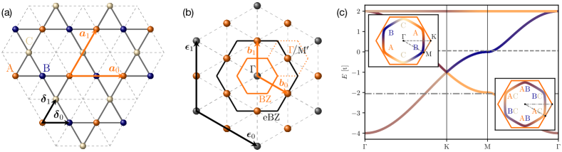
Figure 1: Kagome Fermiology and extended zone scheme. (a) Kagome lattice with sublattices $A$, $B$, and $C$ along with the inter $\mathbf{a}_{0,1}$ and intra $\bm{\delta}_{0,1}$ unit cell vectors. (b) Fourier transform of the kagome lattice with Brillouin zone (BZ) in orange and extended Brillouin zone in black. $M^{\prime}$ points in the eBZ coincide with the $\Gamma$ point in the BZ. (c) The kagome band structure features a flat band and two dispersive bands which display particular eigenstate sublattice distribution according to sublattice interference PhysRevB.86.121105 . p-type (m-type) van Hove fillings are symbolized by dashed (dashed-dotted) lines.

In this Letter, we develop a theory of PDW instability on the kagome lattice. Specifically, the PDW we find does not appear as a parasitic onset order to another electronic instability, but unfolds as part of the leading instability in the particle-particle (pp) channel descending from a pristine kagome metallic state. Furthermore, this PDW state does not break translation symmetry, and, in terms of symmetry classification at the pp instability level, admixes with inplane $d$-wave SC ($d$SC) in the $E_{2}$ irreducible representation of the hexagonal point group $C_{6v}$. The key to disentangle the PDW from the $d$SC contribution is the center of mass dependence of the condensate wave function in the tri-atomic unit cell basis. Here, the PDW component exhibits intra-unit cell modulations while the $d$SC component is uniform. We locate the $E_{2}$-type pp domain in the $U$-$V$ phase diagram in the weak coupling domain, analyze its immanent competition between PDW and $d$SC, and identify the adjacent $E_{2}$-type CDW and $A_{1}$-type SC instabilities.

Kagome Hubbard model (KHM). We start from

$$H=t\sum_{\langle i,j\rangle}\left(c^{\dagger}_{i\sigma}c^{\vphantom{\dagger}}_{j\sigma}+\text{h.c.}\right)+U\sum_{i=1}^{N}n_{i\uparrow}n_{i\downarrow}+{\textstyle{V\over 2}}\sum_{\langle i,j\rangle;\sigma\sigma^{\prime}}n_{i\sigma}n_{j\sigma^{\prime}}\,\text{,}$$ (1)

where $c_{i\sigma}^{\dagger},c_{i\sigma}^{\vphantom{\dagger}}$ denote electron creation and annihilation operators at site $i$ with spin $\sigma$, $n_{i\sigma}=c_{i\sigma}^{\dagger}c_{i\sigma}^{\vphantom{\dagger}}$, and $t$, $U$, and $V$ denote the energy scales of hopping, onsite Hubbard, and NN repulsion, respectively. The kagome lattice depicted in Figure 1a features a non-bipartite lattice of corner-sharing triangles, resulting in three sublattices $A$, $B$, and $C$ as well as Bravais lattice vectors $\mathbf{a}_{0}$ and $\mathbf{a}_{1}$. Alternatively, it can be interpreted as a charge density wave formation at 3/4 filling of an underlying triangular lattice with halved unitcell vectors $\bm{\delta}_{0}$ and $\bm{\delta}_{1}$, where every fourth unoccupied site is projected out. In reciprocal space (Figure 1b), this corresponds to the reduced (orange) and extended (black) Brillouin zone (BZ) spanned by the vectors $\mathbf{b}_{0,1}$ and $\bm{\epsilon}_{0,1}$ according to $\mathbf{b}_{i}^{\intercal}\mathbf{a}_{j}=\bm{\epsilon}_{i}^{\intercal}\bm{\delta}_{j}=2\pi\delta_{ij}$. The three inequivalent van Hove points at the M points in the BZ epitomize a peculiar density of states of differing sublattice occupancy (pure-type (p-type) for the upper and mixed-type (m-type) for the lower van Hove level in Figure 1c) PhysRevB.86.121105 ; PhysRevLett.127.177001 , a generic feature of kagome metals which has been recently confirmed by angle-resolved photoemission spectroscopy (ARPES) kang-sli ; hu-sli . For both m-type and p-type, the mismatch of sublattice support for electronic eigenstates connected by van Hove point nesting triggers SI.

FRG instability analysis. The FRG formulates an ultraviolet to infrared cutoff flow of the two-particle electronic vertex operator $V(\mathbf{k}_{1},\mathbf{k}_{2},\mathbf{k}_{3},\mathbf{k}_{4})c^{\dagger}_{\mathbf{k}_{4}}c^{\dagger}_{\mathbf{k}_{3}}c^{\vphantom{\dagger}}_{\mathbf{k}_{2}}c^{\vphantom{\dagger}}_{\mathbf{k}_{1}}$ as a set of differential equations, where the $\mathbf{k}_{i}$ denote lattice momenta. We employ the FRG in its truncated unity (TU) approximation, where the vertex is separated into three different contributions according to their distinctive transfer momenta , which can be classified as two particle-hole (ph) and a single particle-particle (pp) channel. The complementary vertex momenta are expanded in plane wave formfactors $\phi_{f}(\mathbf{k})=e^{i\mathbf{r}_{f}\mathbf{k}}$ via the Bravais lattice sites $\mathbf{r}_{f}=n\mathbf{a}_{0}+m\mathbf{a}_{1}$, $n,m\in\mathbb{Z}$. For the KHM, any channel vertex function is specified by a 4-tuple of sublattice indices $\{o_{i}\}$, $i=1,2,3,4$, transfer momentum $\mathbf{Q}$, and two residual momenta which we expand into formfactors according to

$$\mathcal{V}^{\{o_{i}\}}_{ff^{\prime}}(\mathbf{Q})=\int_{\text{BZ}}\!\!\!\mathrm{d}\mathbf{k}\mathrm{d}\mathbf{k}^{\prime}V^{\{o_{i}\}}(\mathbf{Q},\mathbf{k},\mathbf{k}^{\prime})\phi_{f}(\mathbf{k})\bar{\phi}_{f^{\prime}}(\mathbf{k}^{\prime})\,\text{.}$$ (2)

Truncating the set of basis functions, reflecting the locality of pp and ph pairs, this unitary expansion becomes approximate. We terminate the flow at an energy scale $\Lambda_{c}$, upon encountering a divergence in a vertex element indicating a symmetry breaking phase transition. At this point, the effective vertex contains all higher energy quantum fluctuations accessible within the FRG approach. For SC pairing at $\mathbf{Q}=0$, the system’s ground state is then obtained from the BCS gap equation which reduces to an eigenvalue problem

$$\lambda\Delta_{o_{1}o_{2}}^{f}=\sum_{f^{\prime}o_{3}o_{4}}\mathcal{V}_{ff^{\prime}}^{\{o_{i}\}}(0)\,\Delta_{o_{3}o_{4}}^{f^{\prime}}$$ (3)

at the onset of ordering. The functional form of the SC order parameter is thus given by the eigenstate $\Delta_{o_{1}o_{2}}^{f}$ associated with the most negative eigenvalue $\lambda$. Exploiting the group symmetry constraints on Eq. (3) along Schur’s lemma allows for a classification of $\Delta_{o_{1}o_{2}}^{f}$ in terms of irreducible representations (irreps) of $C_{6v}$. Within our TUFRG analysis, we identify an extended region in the $U$-$V$ parameter space where $\mathbf{Q}=0$ instabilities in the spin-singlet pp channel dominate, and the superconducting order parameter transforms according to the $E_{2}$ irrep.

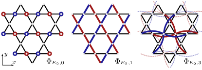
Figure 2: Harmonics of the $E_{2}$ irrep with $y$-mirror eigenvalue $-1$. We show the onsite ($\Phi_{E_{2},0}$), first NN ($\Phi_{E_{2},1}$), and third NN harmonic ($\Phi_{E_{2},3}$). We skip the second NN due to its similarity to the first NN. Red/blue indicates positive/negative value of the pair correlation Eq. (4) between connected sites.

Classification of the $E_{2}$ pp instability. A two-electron expectation value in the spin singlet sector

$$\langle c^{{\dagger}}_{\mathbf{r}_{i},\uparrow}c^{{\dagger}}_{\mathbf{r}_{j},\downarrow}-c^{{\dagger}}_{\mathbf{r}_{j},\uparrow}c^{{\dagger}}_{\mathbf{r}_{i},\downarrow}\rangle=\delta_{\mathbf{r}_{i},\bm{\rho}}\,\delta_{\mathbf{r}_{j},\bm{\rho}}\,\Phi(\mathbf{r}_{i},\mathbf{r}_{j})$$ (4)

is most conveniently described in terms of a center of mass coordinate (CMC) $\mathbf{R}=(\mathbf{r}_{i}+\mathbf{r}_{j})/2$ and a relative coordinate (RC) $\mathbf{r}=\mathbf{r}_{i}-\mathbf{r}_{j}$. In the following, we denote the set of all lattice points by $\bm{\rho}$ and use $\bm{\rho}_{o}$ for points related to sublattice $o\in\{A,B,C\}$. We introduce $\mathbf{a}_{2}=\mathbf{a}_{1}-\mathbf{a}_{0}$ and $\bm{\delta}_{2}=\bm{\delta}_{1}-\bm{\delta}_{0}$ for notational convenience. Since the kagome lattice is not of Bravais type, the directions of NN bonds depend on the sublattice. For each pairing distance, i.e., each value of the RC (onsite, NN, etc.), the $E_{2}$ irrep is expanded in pairs of degenerate orthogonal states, characterized by even or odd transformation behavior under mirror symmetry along the $y$-axis Note1 . We order different $E_{2}$ candidate states by their RC length and constrain ourselves to the mirror-odd state as we present a graphical representation in Figure 2. The onsite ($\mathbf{r}=0$) pairing wave function reads

$$\Phi_{E_{2},0}(\mathbf{R},\mathbf{r})=\Big{(}\delta_{\mathbf{R},\bm{\rho}_{A}}-\delta_{\mathbf{R},\bm{\rho}_{B}}\Big{)}\delta_{\mathbf{r},\mathbf{0}}\,\text{.}$$ (5)

The absence of a lattice site at the point group’s rotation center, allows for such onsite pairing wave functions on any non-Bravais lattice. The trivial transformation property of the RC is complemented by a non-trivial CMC function due to the reduced site symmetry group of the $3c$ Wyckoff position. In contrast, the NN pairing state

$$\Phi_{E_{2},1}(\mathbf{R},\mathbf{r})=\delta_{\mathbf{r},\pm\bm{\delta}_{1}}-\delta_{\mathbf{r},\pm\bm{\delta}_{2}}$$ (6)

features a trivial CMC dependence, and instead it is the RC that captures the $E_{2}$ transformation behaviour. Whereas the second NN state is structurally equivalent Note1 to the NN state, the third NN pairing reads

$$\begin{split}\Phi_{E_{2},3}(\mathbf{R},\mathbf{r})=\,&\delta_{\mathbf{R},\bm{\rho}_{B}}\delta_{\mathbf{r},\pm\mathbf{a}_{0}}-\delta_{\mathbf{R},\bm{\rho}_{A}}\delta_{\mathbf{r},\pm\mathbf{a}_{0}}\\ +\,&\delta_{\mathbf{R},\bm{\rho}_{C}}\Big{(}\delta_{\mathbf{r},\pm\mathbf{a}_{1}}-\delta_{\mathbf{r},\pm\mathbf{a}_{2}}\Big{)}.\end{split}$$ (7)

It cannot be decomposed into a product of solely CMC and RC dependent functions. This stems from two symmetry-inequivalent types of third NN on the kagome lattice due to the reduced $C_{2v}$ site symmetry group, that yields the additional spatial CMC structure Note1 .

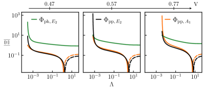
Figure 3: FRG vertex analysis for $U/t=0.14$ and $0.47<V/t<0.77$ as a function of the energy cutoff $\Lambda$. $E_{2}$ CDW ($\Phi_{\text{ph},\,E_{2}}$, green), PDW $E_{2}$ pp order ($\Phi_{\text{pp},\,E_{2}}$, black), and SC $A_{1}$ pp ($\Phi_{\text{pp},\,A_{1}}$, orange) compete for the leading instability. Attractive (repulsive) expectation values $|\Xi|$ of the leading instabilities at $\Lambda_{c}$ are indicated by solid (dashed) lines Note1 .

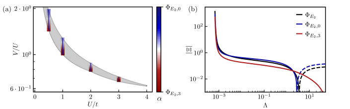
Figure 4: (a) Admixture ratio $\alpha$ of $\Phi_{E_{2},0}$ (blue) (5) and $\Phi_{E_{2},3}$ (red) (7) for the $E_{2}$ pp domain at $n=5/12$. (b) Expectation value of the leading eigenstate at $\Lambda_{c}$ (black), $\Phi_{E_{2},0}$, and $\Phi_{E_{2},3}$. Negative (positive) values are indicated by solid (dashed) lines.

PDW wave function. Two candidate states may belong to the same irrep and yet trace back to entirely different physical origins. For the $A_{1}$ pairing irrep on the square lattice, this has been extensively discussed in the context of $s_{\pm}$ vs. $s_{++}$-wave SC in iron pnictides Hirschfeld_2011 ; doi:10.1146/annurev-conmatphys-020911-125055 . For the kagome lattice, the fundamentally different nature of $E_{2}$ formfactors becomes apparent upon disentangling the spatial information encoded in CMC and RC, respectively. The Cooper pair wave function of typical zero momentum SCs features a uniform CMC dependence, while the RC encodes the transformation behavior of the associated irrep. Eq. (5), however, describes a scenario where the typical roles of CMC and RC are interchanged. It obeys $\sum_{\mathbf{R}}\Phi(\mathbf{R},\mathbf{r})=0$, which is a characteristic of PDW-type pairing Arovas2022 . The key point to appreciate here is that despite the $\mathbf{Q}=0$ channel, spatially modulated contributions can be distinguished from homogeneous ones within the multi-site unit cell. This is the essential difference between the PDW and $d$SC contributions to an $E_{2}$ pp instability in the KHM.

Alternatively, one may interpret the kagome lattice as a ficticious CDW on the triangular lattice at 3/4 filling, restoring the full real space information previously encoded in the sublattice indices of the tri-atomic basis, and the extended BZ reveals finite momentum Cooper pairing long_paper . As a corollary, pairing states which mix SC and PDW such as Eq. (7), i.e., which do not factorize into a CMC and RC part, are also allowed by symmetry. Such states were previously found, yet not adequately appreciated, in the kagome phase diagram of Ref. PhysRevB.87.115135, .

PDW phase domain. Within our TUFRG analysis of the KHM, the $E_{2}$ pp instability domain is governed by intra-sublattice pairing, i.e., the eigenstates of Eq. (3) are described by a linear combination of $\Phi_{E_{2},0}$ and $\Phi_{E_{2},3}$ Note1 . This allows to identify the $E_{2}$ pp instability as a PDW. The intra-sublattice pairing tendency can be understood from the viewpoint of SI: Under the RG, effects of $U$ are suppressed while $V$ grows si-patch , making inter-sublattice pairing less favourable. This trend also manifests in the fact that the PDW instability at small $U/t$ is parametrically framed by an $E_{2}$-type CDW and an $A_{1}$-type, i.e., $s$-wave SC (Figure 3) at p-type van Hove filling.

The PDW state emerges as interstitial order via competing interaction processes projected into the pairing channel: $U$ drives non-local spin fluctuations; $V$, by contrast, generates charge fluctuations entering the Cooper channel as onsite attractive interactions Romer_2022 . In Figure 3, we illustrate the generic scenario of competing instabilities generated by this interplay of local and non-local interactions by comparing FRG flows for varying bare values $0.47<V<0.77$ at fixed $U=0.14$, i.e., located in the weak coupling domain. Both PDW-type and $s$-wave SC channels are initially repulsive (dashed lines) and subsequently turn attractive (solid lines) through the RG flow. Remarkably, the adjacent CDW features the same irrep and intra-sublattice modulation as the PDW phase, suggesting vestigial symmetry-type restoration at the phase transition. In previous contexts, PDW fluctuations were similarly found to predominantly occur around phase transitions between a density wave phase and SC pairing, where a variety of competing and/or cooperative orders arise at intermediate coupling strength doi:10.1146/annurev-conmatphys-031119-050711 . Any weak coupling theory of PDW has hitherto relied on fine-tuned Fermiology wc_PDW . Here, however, we find that the PDW prevails beyond p-type van Hove filling whenever intra-unit cell modulations become competitive to homogeneous pairing functions due to SI.

The competition of interaction processes is directly reflected in the pairing wave functions overlap with $\Phi_{E_{2},0}$ and $\Phi_{E_{2},3}$ Note1 and their relative weight $\alpha$, which is depicted in Figure 4a for the PDW regime at p-type van Hove filling. The third NN state $\Phi_{E_{2},3}$ does not suffer an energy penalty from $U$ in (1) and thus promotes attractive pairing channel already at bare coupling (Figure 4b). Analogous to the previous discussion, $V$-driven intra-unit cell charge fluctuations yield an onsite attraction of Cooper pairs through the RG flow PhysRevB.87.115135 . The onsite contribution $\Phi_{E_{2},0}$ to PDW increases with $V$, and eventually drives the system into an $s$-wave SC.

Conclusion and outlook.

The PDW instability we find for the KHM does not match the roton density wave reported for the kagome metal CsV₃Sb₅ within the $2\times 2$ charge order domain, where the effective unit cell vectors are doubled as compared to $\mathbf{a}_{0,1}$ in Figure 1a roton-pdw . Our findings, however, emphasize the mechanisms leading up to PDW formation in kagome metals. The methodological shortcoming to surmount in the future is to continue the FRG flow into symmetry-broken phases Salmhofer2004 . Our findings expand the microscopic, analytically controlled access to PDW. For the kagome unit cell, the competing character of PDW versus $d$SC becomes most concrete, as the PDW is located in the same irrep as $d$SC. Viewing the kagome lattice as a ficticious 3/4 filling CDW of an underlying triangular lattice (Figure 1a), we recover the expected intertwined character of PDW: the kagome-CDW at $2\bm{\delta}_{1,0}$ comes along with a $2\bm{\delta}_{1,0}$ PDW competing with $d$SC. The $2\times 2$ charge order in kagome metals PhysRevLett.127.217601 would then be the $4\bm{\delta}_{1,0}$ CDW, which is found for a Ginzburg Landau analysis of intertwined PDW order PhysRevB.97.174510 .

Acknowledgement.

We thank S. A. Kivelson, M. Klett, J.M. Hauck, and M. Sigrist for discussions. The work is funded by the Deutsche Forschungsgemeinschaft (DFG, German Research Foundation) through Project-ID 258499086 - SFB 1170 and and through the Würzburg-Dresden Cluster of Excellence on Complexity and Topology in Quantum Matter – ct.qmat Project-ID 390858490 - EXC 2147. We acknowledge HPC resources provided by the Erlangen National High Performance Computing Center (NHR@FAU) of the Friedrich-Alexander-Universität Erlangen-Nürnberg (FAU). NHR funding is provided by federal and Bavarian state authorities. NHR@FAU hardware is partially funded by the DFG – 440719683. M.D. received funding from the European Research Council under Grant No. 771503 (TopMech-Mat). J.B. thanks the DFG for support through RTG 1995 from SPP 244 “2DMP”.

I Supplemental Material

I.1 Truncated Unity FRG

While the natural energy scale of the non-interacting theory is determined by the bandwidth of the single particle spectrum, the situation becomes more delicate in the presence of interactions. Interaction effects establish collective ordering phenomena at energy scale several orders of magnitude below the strength of the bare interaction in the initial Hamiltonian due to screening by the non interacting background. To trace down the effective contribution of interactions to the physics at the important energy scales, a variety of renormalization procedures have been developed to incorporate higher order screening processes in the low energy effective theory.

Among these, the functional renormalization group stands out by its unbiased differentiation of phases and is the natural method for the PDW analysis. While we omit the basics of FRG itself by referencing to the literature doi:10.1080/00018732.2013.862020 ; RevModPhys.84.299 instead, we want to reintroduce the TUFRG LICHTENSTEIN2017100 ; Schober_2018 approximation here: We start out with the integro-differential equation of the functional renormalization group in its SU(2) reduced form:

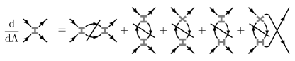
Figure 5: Diagrammatic representation of the SU$(2)$-TUFRG flow. The dash through the pair of propagator lines indicates the derivative w.r.t. the scale $\Lambda$. The diagrams can be separated into the three channels by their transfer momentum between the 2-particle vertices: The first diagram is associated with the $P$-channel, the next three contribute to the $D$-channel and $C$-channel consists of the last diagram.

The exact perturbative expansion of the FRG vertex has already been truncated at the two-particle level to make the infinite hierarchy of coupled equations solvable.

We furthermore exploit spin rotational invariance, which allows to consider the opposite spin channel only. The symmetric and antisymmetric part of the thereby obtained effective interaction resembles the singlet and triplet correlations respectively. For brevity we drop the spin and sublattice indices in all following formulae, which we retain as tensor dimensions of the object $V^{o_{1}o_{2}o_{3}o_{4}}_{\uparrow\downarrow\uparrow\downarrow}(\mathbf{k}_{1},\mathbf{k}_{2},\mathbf{k}_{3})$. The exact order of indices can be inferred from the diagrammatic expression where the shape of the vertices indicates connected sublattices.

We further employ the truncated unity expansion to the FRG which is based on the singular mode paradigms PhysRevB.85.035414 . To this end the vertex is decomposed in the particle-particle (P), direct particle-hole (D), crossed particle-hole (C) channel

$$V=V_{P}+V_{D}+V_{C}\,$$ (8)

according to the three possible diagrammatic transfer momenta $\mathbf{Q}_{P}=\mathbf{k}_{1}+\mathbf{k}_{2}$, $\mathbf{Q}_{D}=\mathbf{k}_{1}-\mathbf{k}_{3}$ and $\mathbf{Q}_{C}=\mathbf{k}_{1}-\mathbf{k}_{4}$. This primary momentum dependence drives any divergence in the channel, so the remaining spatial dependence of any given function $F(\mathbf{k}_{1},\mathbf{k}_{2},\mathbf{k}_{3})$ can be expanded in a suitable set of formfactors $\phi_{f}(\mathbf{k})$ via (more detailed than Eq. (2))

$$\hat{X}[F]_{ff^{\prime}}(\mathbf{Q}_{X})=\int\mathrm{d}\mathbf{k}_{X}\int\mathrm{d}\mathbf{k}^{\prime}_{X}\phi_{f}(\mathbf{k}_{X})\phi_{f^{\prime}}(\mathbf{k}^{\prime}_{X})\\ F\left(\mathbf{k}_{1}(\mathbf{Q}_{X},\mathbf{k}_{X},\mathbf{k}^{\prime}_{X}),\mathbf{k}_{2}(\mathbf{Q}_{X},\mathbf{k}_{X},\mathbf{k}^{\prime}_{X}),\mathbf{k}_{3}(\mathbf{Q}_{X},\mathbf{k}_{X},\mathbf{k}^{\prime}_{X})\right)\,,\\$$ (9)

where $X\in\{P,C,D\}$. Because of the slow-varying nature of the interaction w.r.t. the secondary momenta, the high frequency harmonics can be truncated without significant loss of information. In the present study we choose plane waves $\phi_{f}(\mathbf{k})=e^{-i\mathbf{k}\mathbf{r}_{f}}$ as a complete basis with $\mathbf{r}_{f}$ representing a Bravais lattice site and consider sites up to third nearest neighbors. By applying the above projection to Figure 5, the RG equation for the vertex

$${\textstyle{d\over d\Lambda}}\hat{X}[\mathcal{V}]=\hat{X}[\dot{\mathcal{V}}_{P}]+\hat{X}[\dot{\mathcal{V}}_{D}]+\hat{X}[\dot{\mathcal{V}}_{C}]\,$$ (10)

breaks down to the three separate channel flow equations

$$\begin{split}\hat{P}[\dot{\mathcal{V}}_{P}]_{ff^{\prime}}(\mathbf{Q}_{P})&=\sum_{f_{1},f_{2}}\mathcal{V}_{ff_{1}}(\mathbf{Q}_{P})\dot{L}^{pp}_{f_{1}f_{2}}(\mathbf{Q}_{P})\mathcal{V}_{f_{2}f^{\prime}}(\mathbf{Q}_{P})\\ \hat{D}[\dot{\mathcal{V}}_{D}]_{ff^{\prime}}(\mathbf{Q}_{D})&=\sum_{f_{1},f_{2}}\left[-2\mathcal{V}_{ff_{1}}(\mathbf{Q}_{D})\dot{L}^{ph}_{f_{1}f_{2}}(\mathbf{Q}_{D})\mathcal{V}_{f_{2}f^{\prime}}(\mathbf{Q}_{D})\right.\\ &\qquad+\mathcal{V}_{ff_{1}}(\mathbf{Q}_{C})\dot{L}^{ph}_{f_{1}f_{2}}(\mathbf{Q}_{D})\mathcal{V}_{f_{2}f^{\prime}}(\mathbf{Q}_{D})\\ &\qquad\left.+\mathcal{V}_{ff_{1}}(\mathbf{Q}_{D})\dot{L}^{ph}_{f_{1}f_{2}}(\mathbf{Q}_{D})\mathcal{V}_{f_{2}f^{\prime}}(\mathbf{Q}_{C})\right]\\ \hat{C}[\dot{\mathcal{V}}_{C}]_{ff^{\prime}}(\mathbf{Q}_{C})&=\sum_{f_{1},f_{2}}\mathcal{V}_{ff_{1}}(\mathbf{Q}_{C})\dot{L}^{ph}_{f_{1}f_{2}}(\mathbf{Q}_{C})\mathcal{V}_{f_{2},f^{\prime}}(\mathbf{Q}_{C})\,.\end{split}$$ (11)

Here $\dot{L}^{pp}_{ff^{\prime}}(\mathbf{Q})$ and $\dot{L}^{ph}_{ff^{\prime}}(\mathbf{Q})$ are the product of single-scale propagator and propagator $({\textstyle{dG^{\Lambda}G^{\Lambda}\over d\Lambda}})$ in either particle-particle (pp) or particle-hole (ph) configuration transformed into TU representation.

Since renormalisation effects for each transfer momentum are accumulated separately, the computational complexity of the calculations reduces significantly while retaining momentum conservation which was not possible in the n-patch FRG schemes used previously doi:10.1080/00018732.2013.862020 . Additionally, the full orbital and band space dependencies are kept throughout the RG procedure, since the expansion in Eq. (LABEL:eq:ff_expansion) only effects the momentum quantum numbers. In particular for systems with sublattice, this allows to extract the real space structure within the unit cell from the order parameter at the end of the flow.

We are left with the remaining problem of the cross-channel projections, i.e. the contribution of each $\dot{V}_{X}$ in the two complementary channels. By respecting the interplay between the channels, the TUFRG distinguishes itself from the calculation of three simultaneous but disconnected RPA flows and becomes an unbiased method, which treats propensities towards particle-particle instabilities on equal footing to particle-hole instabilities. The cross channel projections can be reduced to complicated tensor transformations for each pair $X,Y$ from $\{P,C,D\}:X\neq Y$

$$\mathrm{d}\mathcal{V}^{\{o_{i}\}}_{X,ff^{\prime}}(\mathbf{Q}_{X})\\ =\sum_{\mathbf{Q}_{Y}}M^{X,ff^{\prime}}_{Y,f_{1}f_{2}}(\mathbf{Q}_{X},\mathbf{Q}_{Y})\mathrm{d}\mathcal{V}^{\mathcal{P}_{X,Y}[\{o_{i}\}]}_{Y,f_{1}f_{2}}(\mathbf{Q}_{Y})\,.$$ (12)

This set of integro-differential equations and coupling equations can be integrated as it would be in ordinary FRG:

To obtain a log scale theory close to the Fermi level, we start from the free theory at $\Lambda\sim\infty$ and integrate the flow equations towards lower scale. Upon encountering a phase transition one (or more) of the differentials in Eq. (11) diverges at energy scale $\Lambda_{C}$, which can be related to the critical temperature $T_{C}\propto\Lambda_{C}$ of the transition. To associate the divergent channels with physical instabilities, the effective interaction at $\Lambda_{C}$ is transformed back into momentum space and decomposed into the pairing

$$\begin{split}\Gamma_{\text{pp}}=&\sum_{\mathbf{Q}\mathbf{k}\mathbf{k}^{\prime}}\sum_{o_{i}}V^{\{o_{i}\}}_{P}\big{(}\mathbf{Q},\mathbf{k},\mathbf{k}^{\prime}\big{)}\\ &c^{{\dagger}}_{\mathbf{k}+\mathbf{Q}/2,o_{2}\uparrow}c^{{\dagger}}_{-\mathbf{k}+\mathbf{Q}/2,o_{3}\downarrow}c^{\vphantom{{\dagger}}}_{-\mathbf{k}^{\prime}+\mathbf{Q}/2,o_{1}\downarrow}c^{\vphantom{{\dagger}}}_{\mathbf{k}^{\prime}+\mathbf{Q}/2,o_{0}\uparrow},\end{split}$$ (13)

charge

$$\begin{split}\Gamma_{\text{cha}}=&\sum_{\mathbf{Q}\mathbf{k}\mathbf{k}^{\prime}}\sum_{o_{i}ss^{\prime}}\left[V^{\{o_{i}\}}_{D}\big{(}\mathbf{Q},\mathbf{k},\mathbf{k}^{\prime}\big{)}-{\textstyle{1\over 2}}V^{o_{0}o_{1}o_{3}o_{2}}_{C}\big{(}\mathbf{Q},\mathbf{k},\mathbf{k}^{\prime}\big{)}\right]\\ &c^{{\dagger}}_{\mathbf{k}-\mathbf{Q}/2,o_{2}s}c^{\vphantom{{\dagger}}}_{\mathbf{k}+\mathbf{Q}/2,o_{0}s}c^{{\dagger}}_{\mathbf{k}^{\prime}+\mathbf{Q}/2,o_{3}s^{\prime}}c^{\vphantom{{\dagger}}}_{\mathbf{k}^{\prime}-\mathbf{Q}/2,o_{1}s^{\prime}},\end{split}$$ (14)

and magnetic

$$\begin{split}\Gamma_{\text{mag}}=&\sum_{\mathbf{Q}\mathbf{k}\mathbf{k}^{\prime}}\sum_{\{o_{i}\}\{s_{i}\}}-V^{\{o_{i}\}}_{C}\big{(}\mathbf{Q},\mathbf{k},\mathbf{k}^{\prime}\big{)}\sigma^{z}_{s_{0}s_{2}}\sigma^{z}_{s_{1}s_{3}}\\ &c^{{\dagger}}_{\mathbf{k}^{\prime}+\mathbf{Q}/2,o_{2}s_{2}}c^{\vphantom{{\dagger}}}_{\mathbf{k}+\mathbf{Q}/2,o_{0}s_{0}}c^{{\dagger}}_{\mathbf{k}-\mathbf{Q}/2,o_{3}s_{3}}c^{\vphantom{{\dagger}}}_{\mathbf{k}^{\prime}-\mathbf{Q}/2,o_{1}s_{1}}\end{split}$$ (15)

contributions LICHTENSTEIN2017100 ; Huseman_Honerkamp . Each renormalized interaction in momentum space is obtained from the quantities in Eq. (11) via the inverse of Eq. (LABEL:eq:ff_expansion), $\sigma^{z}$ is the third Pauli matrix. Since the magnetic channel is not further discussed in the weak coupling domain of PDW elaborated on in the main article, “cha” is abbreviated by “ph” for notational convenience.

From the effective vertex in the most divergent channel, the functional dependence of the order parameter can be analysed by a subsequent mean field (MF) decomposition of the residual interaction term doi:10.1080/00018732.2013.862020 ; metzner_MF1 ; metzner_MF2 . Subsequently, we focus on the pairing channel at $\mathbf{Q}_{P}=0$, which characterises superconductivity and pair density wave formation. An analogous procedure yields the order parameter of adjacent phases like charge and spin density waves and bond orders.

We start by introducing the non vanishing expectation value

$$\Delta(\mathbf{k})={\textstyle{1\over N}}\sum_{\mathbf{k}^{\prime}}\Gamma_{P}(\mathbf{k},\mathbf{k}^{\prime})\langle c^{\vphantom{{\dagger}}}_{\downarrow}(-\mathbf{k}^{\prime})c^{\vphantom{{\dagger}}}_{\uparrow}(\mathbf{k}^{\prime})\rangle$$ (16)

with $\mathbf{k},\mathbf{k}^{\prime}$ restricted to energy scales below the cutoff, i.e. the single particle energies satisfy $|\xi_{n}(\mathbf{k})|<\Lambda_{C}\sim 10^{-4}t$. Assuming no accidental band degeneracies at the Fermi level, this allows a unique mapping between momentum and band quantum number and we hence drop the latter one. Neglecting second order fluctuations around the MF solution, the free energy of the system can be obtained in terms of the eigenspectrum of the Bogoliubov quasiparticles $\xi(\mathbf{k})=\sqrt{E(\mathbf{k})^{2}+|\Delta(\mathbf{k})|^{2}}$ as

$$\begin{split}F=&-T\sum_{\mathbf{k}}\ln\left(1+e^{-\beta\xi(\mathbf{k})}\right)-{\textstyle{1\over 2}}\sum_{\mathbf{k}}\left(\xi(\mathbf{k})-E(\mathbf{k})\right)\\ &+{\textstyle{1\over 2}}\sum_{\mathbf{k}}{\textstyle{|\Delta(\mathbf{k})|^{2}\over 2\xi(\mathbf{k})}}\tanh\left({\textstyle{\xi(\mathbf{k})\over 2T}}\right)\,.\end{split}$$ (17)

Its minimization w.r.t. the order parameter gives the BCS gap equation

$$\Delta(\mathbf{k})=-{\textstyle{1\over N}}\sum_{\mathbf{k}^{\prime}}\Gamma_{P}(\mathbf{k},\mathbf{k}^{\prime}){\textstyle{\Delta(\mathbf{k}^{\prime})\over 2\xi(\mathbf{k}^{\prime})}}\tanh\left({\textstyle{\xi(\mathbf{k}^{\prime})\over 2T}}\right)\,.$$ (18)

Since the FRG flow breaks down at the onset of a phase transition, the appropriate temperature scale at the end of the flow is given by $T_{C}$, which implies $\Delta\rightarrow 0$. Thus, the righthand side of the above equation can be expanded to first order in the order parameter. From the linearised version of Eq. (18),

$$\lambda\Delta(\mathbf{k})={\textstyle{1\over N}}\sum_{\mathbf{k}^{\prime}}\Gamma_{P}(\mathbf{k},\mathbf{k}^{\prime})\Delta(\mathbf{k}^{\prime})\,,$$ (19)

the spatial dependence of the order parameter is given by the eigenstate of $\Gamma_{P}$ associated with the most negative eigenvalue $\lambda$. In the case of degenerate leading pairing eigenvalues, the system will realise the complex superposition of the degenerate modes, that minimizes the free energy in Eq. (17).

The analysis of many body instabilities in the low energy effective theory obtained by the TU FRG workflow will be detailed in an upcoming paper long_paper .

I.1.1 Vertex symmetrization routine

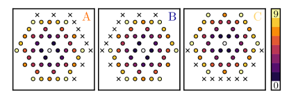
Figure 6: Resymmetrization of formfactor expansion. When calculating in proper gauge we implicitly mix different distances in the truncation of the formfactor expansion in Eq. LABEL:eq:ff_expansion. To circumvent the thereby induced symmetry breaking, the formfactor basis has to be adjusted for each sublattice individually to suffice the site symmetry group $C_{2v}$. Sites x do not have a symmetry partner w.r.t the central site and are therefore discarded.

For computational convenience, the FRG treatment of the effective vertex is usually performed in proper gauge as describe in Ref. Beyer2022 : To maintain a periodic Hamiltonian w.r.t. the reciprocal lattice vectors, we choose a gauge where all sites $o$ within the unit cell ($o\in\{$A,B,C$\}$) are transformed respective the origin of the unit cell

$$c_{i,o}=\int_{\text{BZ}}\!d\mathbf{k}e^{\mathrm{i}\mathbf{k}\mathbf{r}_{i}}c_{\mathbf{k},o}\,,$$ (20)

with $\mathbf{r}_{i}=n\mathbf{a}_{0}+m\mathbf{a}_{1},$ and $n,m\in\mathbb{Z}$ as opposed to the improper and non-periodic form

$$c_{i,o}=\int_{\text{BZ}}\!d\mathbf{k}e^{\mathrm{i}\mathbf{k(}\mathbf{r}_{i}+\mathbf{r}_{o})}c_{\mathbf{k},o}\,,$$ (21)

where they are transformed respective their position. $\mathbf{r}_{o}$ denotes the shift from the unit cell origin to the position of sublattice $o$. Thus, $(\mathbf{r}_{i}+\mathbf{r}_{o})$ are all lattice vectors of the Kagome lattice. The formfactor expansion in LABEL:eq:ff_expansion considers only a finite number of formfactors, which is defined by the number of formfactor shells ($n_{\text{shell}}$) around the onsite unit cell. This induces a truncation of neighboring real-space sites $\{\mathbf{r}_{i}:|\mathbf{r}_{i}|\leq d_{n}\}$, where $d_{n}$ is the distance between onsite- and $n_{\text{shell}}$-NN unit cell. This is sufficient for intra-orbital terms. However, for inter-orbital contributions the different sublattice positions $\mathbf{r}_{o}$ within a unit cell mix differing length scales Beyer2022 . Now $\exists\,\mathbf{r}_{i,o}:|\mathbf{r}_{i}+\mathbf{r}_{o}|>d_{n}$ and those elements break the symmetry of the system as the unit cell orientation favors one direction. An illustration of all sites contained in the formfactor expansion up to third-NN unit cells can be found in Fig. 6. To restore the symmetry we set elements that do not have a symmetry partner w.r.t. the central site (white) to zero in both, the scale derivatives of the propagators, and the effective interactions in each iteration of the FRG flow.

I.2 Complementing basis states of the $E_{2}$ irrep

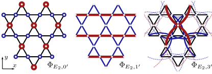
Figure 7: Orthogonal complement of the onsite ($\Phi_{E_{2},0^{\prime}}$), nearest neighbor ($\Phi_{E_{2},1^{\prime}}$), and third nearest neighbor ($\Phi_{E_{2},3^{\prime}}$) pairing states presented in Figure 2 with $y$-mirror eigenvalue $+1$ (“even”). Red/blue indicates positive/negative value of the pair correlation Eq. (4) between connected sites. The thickness of the lines symbolizes the magnitude of pair correlations (red: +2, blue: -1). For $\Phi_{E_{2},3^{\prime}}$ only the connections to the central unit cell are highlighted to preserve visual clarity.

In the main text the set of all lattice sites is referred to as $\bm{\rho}$ while subsets are denoted as $\bm{\rho}_{i}$. With this we can define the lattice constraint factors $\delta_{\mathbf{R},\bm{\rho}}$ as

$$\delta_{\mathbf{R},\bm{\rho}}\equiv\sum_{n,m\in\mathbb{Z}}\sum_{o}\delta_{\mathbf{R},n\mathbf{a}_{0}+m\mathbf{a}_{1}+\mathbf{r}_{o}},$$ (22)

where $\mathbf{r}_{o}$ with $o\in A,B,C$ denotes the positions of the atoms $A,B$ and $C$ in the unit cell with $n,m\in\mathbb{Z}$. The subset of one type of sublattice thus follows as

$$\delta_{\mathbf{R},\bm{\rho}_{o}}\equiv\sum_{n,m\in\mathbb{Z}}\delta_{\mathbf{R},n\mathbf{a}_{0}+m\mathbf{a}_{1}+\mathbf{r}_{o}}.$$ (23)

Another relevant subset consists of the corresponding closest centerpoints of a hexagon to a lattice site. We will denote it as $\bm{\rho}_{A}\pm\bm{\delta}_{2}$, $\bm{\rho}_{B}\pm\bm{\delta}_{1}$ and $\bm{\rho}_{C}\pm\bm{\delta}_{0}$, which are always the sites not present in the kagome lattice. For the $A$ sites this results in

$$\delta_{\mathbf{R},\bm{\rho}_{A}\pm\bm{\delta}_{2}}\equiv\sum_{n,m\in\mathbb{Z}}\delta_{\mathbf{R},n\mathbf{a}_{0}+m\mathbf{a}_{1}+\mathbf{r}_{A}\pm\mathbf{\delta_{2}}}.$$ (24)

The other two terms follow similarly. Various other subsets can be constructed in a similar fashion if needed. With this we are able to separate the inherent translation breaking of the kagome lattice via $\delta_{\mathbf{r}_{k},\bm{\rho}}$. The additional spatial structure induced by the emergent phase in Equation 4 unveils the character of the instability.

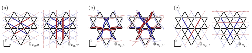
Figure 8: Complementing $E_{2}$ pairing states of the kagome lattice up to third nearest-neighbor. (a) Next nearest-neighbor paring states with odd ($\Phi_{E_{2},2}$) and even ($\Phi_{E_{2},2^{\prime}}$) transformation property w.r.t. a $y$-mirror. (b) and (c) correspond to third nearest-neighbor paring states whereas ($\Phi_{E_{2},\bar{3}}$) and ($\Phi_{E_{2},\bar{3}^{\prime}}$) are formed by connections along the chains of the lattice while ($\Phi_{E_{2},d}$) and ($\Phi_{E_{2},d^{\prime}}$) establish a link across the hexagons. Red/blue indicates the sign (+/-) for the pair correlation in Eq. (4). The magnitude of pair correlations ($\pm 1$ or $\pm 2$) is symbolized by the thickness of the lines. Connections to the central unit cell are highlighted for visual clarity.

In the main text we chose the mirror symmetry along the $y$-axis as a tool to differentiate the two degenerate states transforming under the $E_{2}$ irrep. In detail, this mirror symmetry maps all $C$ sites onto themselves while $A$ and $B$ sites are switched. From this, one can determine two additional symmetry operations that could equally have been chosen for our classification, namely $A\leftrightarrow C$ or $B\leftrightarrow C$. Since they are symmetry equivalent it suffices to only consider one of them.

I.2.1 Harmonic expansion

In this section we show the orthogonal states corresponding to the ones displayed in the main paper and complement these with the remaining states transforming under the $E_{2}$ irrep up to third nearest neighboring sites. A detailed analysis of their contributions is given which validates our restriction to $\Phi_{E_{0}}$ and $\Phi_{E_{3}}$ as the main contributions of the FRG state. The next nearest neighbor correlation state

$$\Phi_{E_{2},2}(\mathbf{R},\mathbf{r})=\delta_{\mathbf{r},\pm(\bm{\delta}_{0}+\bm{\delta}_{1})}-\delta_{\mathbf{r},\pm(\bm{\delta}_{0}-\bm{\delta}_{2})},$$ (25)

is structurally similar to $\Phi_{E_{2},1}$, since it only consists of a relative coordinate (RC) dependence due to the center of mass coordinate (CMC) being already accounted for by the lattice constraint in Eq. (4). In the third nearest neighbor shell, the number of sites exceeds the rank of the point group, which promotes two additional types of third nearest neighbor states:

$$\begin{split}\Phi_{E_{2},\bar{3}}(\mathbf{R},\mathbf{r})=\,&\delta_{\mathbf{R},\bm{\rho}_{B}}\delta_{\mathbf{r},\pm\mathbf{a}_{0}}+\delta_{\mathbf{R},\bm{\rho}_{A}}\delta_{\mathbf{r},\pm\mathbf{a}_{0}}\\ -\,&\delta_{\mathbf{R},\bm{\rho}_{C}}\Big{(}\delta_{\mathbf{r},\pm\mathbf{a}_{1}}+\delta_{\mathbf{r},\pm\mathbf{a}_{2}}\Big{)}.\end{split}$$ (26)

is symmetric under a mirror operation along the $y$-axis and thus perpendicular to $\Phi_{E_{2},3}$. The second state

$$\begin{split}\Phi_{E_{2},d}(\mathbf{R},\mathbf{r})=\,&\delta_{\mathbf{R},\bm{\rho}_{A}\pm\bm{\delta}_{2}}\delta_{\mathbf{r},\pm\mathbf{a}_{2}}-\delta_{\mathbf{R},\bm{\rho}_{B}\pm\bm{\delta}_{1}}\delta_{\mathbf{r},\pm\mathbf{a}_{1}}.\end{split}$$ (27)

is not symmetry equivalent to the $\Phi_{E_{2},3}$ and $\Phi_{E_{2},\bar{3}}$ states since the CMC coordinate always lies in the hexagon center of the kagome lattice, i.e. an empty site. Due to this we call it the $E_{2},d$ where the $d$ stands for diagonal. Another difference to the $\Phi_{E_{2},3}/\Phi_{E_{2},\bar{3}}$ states, is that the pairing sites have two intermediate sites as opposed to one, which decreases the relative contribution of the $\Phi_{E_{2},d}$ state. The associated states with opposite transformation behavior under mirroring along the $y$-axis complete the basis set for the $E_{2}$. These will be denoted by $\Phi_{E_{2},i^{\prime}}$. For the onsite state $\Phi_{E_{2},0}$ we get

$$\Phi_{E_{2},0^{\prime}}(\mathbf{R},\mathbf{r})=\delta_{\mathbf{r},\mathbf{0}}\Big{(}+2\delta_{\mathbf{R},\bm{\rho}_{C}}-\delta_{\mathbf{R},\bm{\rho}_{B}}-\delta_{\mathbf{R},\bm{\rho}_{A}}\Big{)}\,\text{.}$$ (28)

The corresponding orthogonal states to $\Phi_{E_{2},1}$ and $\Phi_{E_{2},2}$ read

$$\Phi_{E_{2},1^{\prime}}(\mathbf{R},\mathbf{r}) =2\delta_{\mathbf{r},\pm\bm{\delta}_{0}}-\delta_{\mathbf{r},\pm\bm{\delta}_{1}}-\delta_{\mathbf{r},\pm\bm{\delta}_{2}}\,\text{,}$$ (29)

$$\Phi_{E_{2},2^{\prime}}(\mathbf{R},\mathbf{r}) =2\delta_{\mathbf{r},\pm(\bm{\delta}_{1}+\bm{\delta}_{2})}-\delta_{\mathbf{r},\pm(\bm{\delta}_{0}+\bm{\delta}_{1})}-\delta_{\mathbf{r},\pm(\bm{\delta}_{0}-\bm{\delta}_{2})}\,\text{.}$$ (30)

The $\Phi_{E_{2},3^{\prime}}$ state, which transforms even under mirroring along the $y$-axis, has the same properties as it’s orthogonal counterpart in that it does not factorize into CMC and RC components

$$\begin{split}\Phi_{E_{2},3^{\prime}}(\mathbf{R},\mathbf{r})=&+2\,\big{(}\delta_{\mathbf{R},\bm{\rho}_{A}}\delta_{\mathbf{r},\pm\mathbf{a}_{1}}+\delta_{\mathbf{R},\bm{\rho}_{B}}\delta_{\mathbf{r},\pm\mathbf{a}_{2}}\big{)}\\ &-\phantom{2}\,\big{(}\delta_{\mathbf{R},\bm{\rho}_{C}}\delta_{\mathbf{r},\pm\mathbf{a}_{2}}+\delta_{\mathbf{R},\bm{\rho}_{A}}\delta_{\mathbf{r},\pm\mathbf{a}_{0}}\big{)}\\ &-\phantom{2}\,\big{(}\delta_{\mathbf{R},\bm{\rho}_{B}}\delta_{\mathbf{r},\pm\mathbf{a}_{0}}+\delta_{\mathbf{R},\bm{\rho}_{C}}\delta_{\mathbf{r},\pm\mathbf{a}_{1}}\big{)}.\end{split}$$ (31)

The same holds for $\Phi_{E_{2},\bar{3}^{\prime}}$

$$\begin{split}\Phi_{E_{2},\bar{3}^{\prime}}(\mathbf{R},\mathbf{r})=&+2\,\big{(}\delta_{\mathbf{R},\bm{\rho}_{A}}\delta_{\mathbf{r},\pm\mathbf{a}_{1}}-\delta_{\mathbf{R},\bm{\rho}_{B}}\delta_{\mathbf{r},\pm\mathbf{a}_{2}}\big{)}\\ &-\phantom{2}\,\big{(}\delta_{\mathbf{R},\bm{\rho}_{C}}\delta_{\mathbf{r},\pm\mathbf{a}_{2}}-\delta_{\mathbf{R},\bm{\rho}_{A}}\delta_{\mathbf{r},\pm\mathbf{a}_{0}}\big{)}\\ &-\phantom{2}\,\big{(}\delta_{\mathbf{R},\bm{\rho}_{B}}\delta_{\mathbf{r},\pm\mathbf{a}_{0}}-\delta_{\mathbf{R},\bm{\rho}_{C}}\delta_{\mathbf{r},\pm\mathbf{a}_{1}}\big{)},\end{split}$$ (32)

which transforms odd under a mirror operation along the $y$-axis. Lastly we have the even counterpart to $\Phi_{E_{2},d}$

$$\begin{split}\Phi_{E_{2},d^{\prime}}(\mathbf{R},\mathbf{r})=\,&+2\delta_{\mathbf{R},\bm{\rho}_{C}\pm\bm{\delta}_{0}}\delta_{\mathbf{r},\pm\mathbf{a}_{0}}\\ &-\phantom{2}\delta_{\mathbf{R},\bm{\rho}_{B}\pm\bm{\delta}_{1}}\delta_{\mathbf{r},\pm\mathbf{a}_{1}}\\ &-\phantom{2}\delta_{\mathbf{R},\bm{\rho}_{A}\pm\bm{\delta}_{2}}\delta_{\mathbf{r},\pm\mathbf{a}_{2}}.\end{split}$$ (33)

which also does not factorize into CMC and RC. The real space representations of the states are shown in Figure 7, Figure 8.

I.3 Candidate state analysis of FRG results

In order to trace the competing contributions within the FRG flow, i.e. as a function of energy cutoff $\Lambda$, we determine the expectation value

$$\Xi\,=\,\braket{\Phi_{\nu,\theta}}{\,V_{\nu}\,}{\Phi_{\nu,\theta}}$$ (34)

of the effective FRG vertex $V_{\nu}$ at each flow step. $\nu\in\,$(pp, cha, mag) denotes the physical instability channels reconstructed from the TUFRG decomposition in Eq. (13), (14), (15). $\theta$ defines the candidate state, for which we take the final FRG state of the respective phases in Figure 3 and the PDW trial states in Figure 4.

To calculate the overlaps of the FRG state with the candidate states we define

$$\gamma_{E_{2},i}=|\braket{\Psi_{\text{FRG}}}{\Phi_{E_{2},i}}|^{2}+|\braket{\Psi_{\text{FRG}}}{\Phi_{E_{2},i^{\prime}}}|^{2}.$$ (35)

As shown in Table 1, the FRG state is predominantly composed of $\Phi_{E_{2},0}$ and $\Phi_{E_{2},3}$. When increasing the nearest-neighbor repulsion $V$, the ratio $\Phi_{E_{2},3}/\Phi_{E_{2},0}$ declines as longer-ranged fluctuations are suppressed. To highlight this fact we define the ratio

$$\alpha\,=\,\dfrac{1}{2}+\dfrac{1}{2}\,\dfrac{\gamma_{E_{2},0}-\gamma_{E_{2},3}}{\gamma_{E_{2},0}+\gamma_{E_{2},3}}$$ (36)

resulting in $\alpha=0$ ($\alpha=1$) for a pure $\Phi_{E_{2},3}$ ($\Phi_{E_{2},0}$) contribution.

$V/t$	$\gamma_{E_{2},0}$	$\gamma_{E_{2},1}$	$\gamma_{E_{2},2}$	$\gamma_{E_{2},3}$	$\gamma_{E_{2},d}$	$\gamma_{E_{2},\bar{3}}$	$\gamma_{A_{1}}$	$\Sigma$
0.50	50.86	0.00	0.55	43.76	0.11	0.01	0.0	95.31
0.52	53.75	0.00	0.60	41.47	0.04	0.01	0.0	95.87
0.54	56.13	0.00	0.63	39.44	0.01	0.01	0.0	96.23
0.56	58.18	0.00	0.66	37.63	0.00	0.01	0.0	96.49
0.58	59.95	0.00	0.69	36.02	0.00	0.01	0.0	96.68
0.60	61.53	0.00	0.72	34.57	0.01	0.01	0.0	96.84
0.62	62.92	0.00	0.74	33.25	0.03	0.01	0.0	96.97
0.64	64.18	0.00	0.77	32.05	0.06	0.02	0.0	97.07
0.66	65.29	0.01	0.80	30.96	0.09	0.02	0.0	97.16
0.68	66.30	0.01	0.82	29.95	0.13	0.02	0.0	97.22
0.70	0.0	0.0	0.0	0.0	0.0	0.0	80.21	80.21
0.72	0.0	0.0	0.0	0.0	0.0	0.0	80.82	80.82

Table 1: Overlap of the final FRG state (pp channel) with candidate states at $U=0.14$ in percent. Values are calculated according to Equation 35.

References

- (1) D. F. Agterberg et al., Annual Review of Condensed Matter Physics 11, 231 (2020).
- (2) E. Fradkin, S. A. Kivelson, and J. M. Tranquada, Rev. Mod. Phys. 87, 457 (2015).
- (3) P. Fulde and R. A. Ferrell, Phys. Rev. 135, A550 (1964).
- (4) A. I. Larkin and Y. N. Ovchinnikov, Sov. Phys. JETP 20, 762 (1965).
- (5) F. Loder, A. P. Kampf, and T. Kopp, Phys. Rev. B 81, 020511 (2010).
- (6) E. Berg, E. Fradkin, and S. A. Kivelson, Nature Physics 5, 830 (2009).
- (7) D. F. Agterberg and H. Tsunetsugu, Nature Physics 4, 639 (2008).
- (8) P. A. Lee, Phys. Rev. X 4, 031017 (2014).
- (9) Y.-M. Wu, P. A. Nosov, A. A. Patel, and S. Raghu, Phys. Rev. Lett. 130, 026001 (2023).
- (10) W. Metzner, M. Salmhofer, C. Honerkamp, V. Meden, and K. Schönhammer, Rev. Mod. Phys. 84, 299 (2012).
- (11) F. Wang, H. Zhai, Y. Ran, A. Vishwanath, and D.-H. Lee, Phys. Rev. Lett. 102, 047005 (2009).
- (12) C. Platt, W. Hanke, and R. Thomale, Advances in Physics 62, 453 (2013).
- (13) M. L. Kiesel, C. Platt, and R. Thomale, Phys. Rev. Lett. 110, 126405 (2013).
- (14) W.-S. Wang, Z.-Z. Li, Y.-Y. Xiang, and Q.-H. Wang, Phys. Rev. B 87, 115135 (2013).
- (15) M. L. Kiesel and R. Thomale, Phys. Rev. B 86, 121105 (2012).
- (16) Y.-M. Wu, R. Thomale, and S. Raghu, Sublattice Interference promotes Pair Density Wave order in Kagome Metals, 2022.
- (17) X. Wu et al., Phys. Rev. Lett. 127, 177001 (2021).
- (18) M. Kang et al., Nature Physics 18, 301 (2022).
- (19) Y. Hu et al., Nature Communications 13, 2220 (2022).
- (20) See Supplemental Material for details on TUFRG and further basis states.
- (21) P. J. Hirschfeld, M. M. Korshunov, and I. I. Mazin, Reports on Progress in Physics 74, 124508 (2011).
- (22) A. Chubukov, Annual Review of Condensed Matter Physics 3, 57 (2012).
- (23) D. P. Arovas, E. Berg, S. A. Kivelson, and S. Raghu, Annual Review of Condensed Matter Physics 13, 239 (2022).
- (24) R. Thomale and et al., in preparation (2023).
- (25) A. T. Rømer, S. Bhattacharyya, R. Valentí , M. H. Christensen, and B. M. Andersen, Physical Review B 106, (2022).
- (26) D. Shaffer, F. J. Burnell, and R. M. Fernandes, Weak-Coupling Theory of Pair Density-Wave Instabilities in Transition Metal Dichalcogenides, 2022.
- (27) H. Chen et al., Nature 599, 222 (2021).
- (28) M. Salmhofer, C. Honerkamp, W. Metzner, and O. Lauscher, Progress of Theoretical Physics 112, 943 (2004).
- (29) M. M. Denner, R. Thomale, and T. Neupert, Phys. Rev. Lett. 127, 217601 (2021).
- (30) Y. Wang et al., Phys. Rev. B 97, 174510 (2018).
- (31) J. Lichtenstein et al., Computer Physics Communications 213, 100 (2017).
- (32) G. A. H. Schober, J. Ehrlich, T. Reckling, and C. Honerkamp, Frontiers in Physics 6, (2018).
- (33) W.-S. Wang et al., Phys. Rev. B 85, 035414 (2012).
- (34) C. Husemann and M. Salmhofer, Phys. Rev. B 79, 195125 (2009).
- (35) J. Reiss, D. Rohe, and W. Metzner, Phys. Rev. B 75, 075110 (2007).
- (36) W. Metzner and H. Yamase, Phys. Rev. B 100, 014504 (2019).
- (37) J. Beyer, J. B. Hauck, and L. Klebl, The European Physical Journal B 95, 65 (2022).