PersonNeRF :
Personalized Reconstruction from Photo Collections

Abstract

We present PersonNeRF  a method that takes a collection of photos of a subject (e.g. Roger Federer) captured across multiple years with arbitrary body poses and appearances, and enables rendering the subject with arbitrary novel combinations of viewpoint, body pose, and appearance. PersonNeRF builds a customized neural volumetric 3D model of the subject that is able to render an entire space spanned by camera viewpoint, body pose, and appearance. A central challenge in this task is dealing with sparse observations; a given body pose is likely only observed by a single viewpoint with a single appearance, and a given appearance is only observed under a handful of different body poses. We address this issue by recovering a canonical T-pose neural volumetric representation of the subject that allows for changing appearance across different observations, but uses a shared pose-dependent motion field across all observations. We demonstrate that this approach, along with regularization of the recovered volumetric geometry to encourage smoothness, is able to recover a model that renders compelling images from novel combinations of viewpoint, pose, and appearance from these challenging unstructured photo collections, outperforming prior work for free-viewpoint human rendering.

Figure 1: Given a photo collection of a subject (e.g., Roger Federer) (a), our method PersonNeRF builds a space of the subject spanned by camera view, body pose, and appearance (b). PersonNeRF enables traversing this space and exploring unobserved combinations of these attributes (c). Here we render novel views (top row), various body poses (middle row), and different appearances (bottom row) by traversing the corresponding axes. Among all of the renderings shown here, only the central images of rows correspond to a photo actually observed in the training data (corresponding input photo marked with a red square). Photo credits to Getty Images.

1 Introduction

We present a method for transforming an unstructured personal photo collection, containing images spanning multiple years with different outfits, appearances, and body poses, into a 3D representation of the subject. Our system, which we call PersonNeRF  enables us to render the subject under novel unobserved combinations of camera viewpoint, body pose, and appearance.

Free-viewpoint rendering from unstructured photos is a particularly challenging task because a photo collection can contain images at different times where the subject has different clothing and appearance. Furthermore, we only have access to a handful of images for each appearance, so it is unlikely that all regions of the body would be well-observed for any given appearance. In addition, any given body pose is likely observed from just a single or very few camera viewpoints.

We address this challenging scenario of sparse viewpoint and pose observations with changing appearance by modeling a single canonical-pose neural volumetric representation that uses a shared motion weight field to describe how the canonical volume deforms with changes in body pose, all conditioned on appearance-dependent latent vectors. Our key insight is that although the observed body poses have different appearances across the photo collection, they should all be explained by a common motion model since they all come from the same person. Furthermore, although the appearances of a subject can vary across the photo collection, they all share common properties such as symmetry so embedding appearance in a shared latent space can help the model learn useful priors.

To this end, we build our work on top of HumanNeRF [46], which is a state-of-the-art free-viewpoint human rendering approach that requires hundreds of images of a subject without clothing or appearance changes. Along with regularization, we extend HumanNeRF to account for sparse observations as well as enable modeling diverse appearances. Finally, we build an entire personalized space spanned by camera view, body pose, and appearance that allows intuitive exploration of arbitrary novel combinations of these attributes (as shown in Fig. 1).

2 Related Work

3D reconstruction from unstructured photos

Reconstructing static scenes from unstructured photo collections is a longstanding research problem in the fields of computer vision and graphics. The seminal Photo Tourism system [39] applies large-scale structure-from-motion [36] to tourist photos of famous sites, enabling interactive navigation of the 3D scene. Subsequent works leveraged multi-view stereo [37, 10] to increase the 3D reconstruction quality [38, 1]. Recently, this problem has been revisited with neural rendering [43, 44, 30, 19, 40]. In particular, Neural Radiance Fields (NeRFs) [32] have enabled photorealistic view synthesis results of challenging scenes, including tourist sites [27] and even city-scale scenes [42]. In addition to static scenes, unstructured photo collections have been also used to model human faces [15, 20] or even visualize scene changes through time [24, 25, 29].

Our method builds on top of NeRF’s neural volumetric representation of static scenes, and extends it to model dynamic human bodies from unstructured photo collections.

3D reconstruction of humans

Many early works in image-based rendering [41] have addressed the task of rendering novel views of human bodies. These techniques are largely based on view-dependent texture mapping [7], which reprojects observed images into each novel viewpoint using a proxy geometry. The image-based rendering community has explored many geometry proxies for rendering humans, including depth maps [49, 14], visual hulls [28], and parametric human models [3]. An alternative technique for 3D reconstruction and rendering of humans is to use 3D scanning techniques to recover a signed distance field representation [6, 9], and then extract and texture a polygon mesh [11, 5, 26]. Recently, neural field representations [47], have become popular for modeling humans since they are suited for representing surfaces with arbitrary topology. Methods have reconstructed neural field representations of humans from a variety of different inputs, including 3D scans[45, 4, 23, 31, 35], multi-view RGB observations[34, 18, 21], RGB-D sequences[8], or monocular videos [46, 13]. Our work is most closely related to HumanNeRF [46], which reconstructs a volumetric neural field from a monocular video of a moving human. We build upon this representation and extend it to enable reconstructing a neural volumetric model from unstructured photo collections with diverse poses and appearances.

3 Method

In this section, we first review HumanNeRF [46] (Sec. 3.1), explain how we regularize it to improve reconstruction from sparse inputs (Sec. 3.2), and then describe how we model diverse appearances (Sec. 3.3 and 3.4). Finally, we describe how we build a personalized space to support intuitive exploration (Sec. 3.5).

Figure 2: Given an input personal photo collection, our method optimizes for a canonical volume that can render diverse appearances. We represent the canonical volume with an MLP conditioned on an appearance embedding, and use a shared pose-dependent motion field that maps from observation to canonical space. Additionally, we use a pose correction MLP that takes the estimated body pose and a pose embedding and outputs appearance-dependent pose residuals. Finally, to improve rendering quality from sparse observations, we regularize the volumetric representation to have smooth and opaque geometry with $\mathcal{L}_{\rm geom}$ and $\mathcal{L}_{\rm opacity}$, which we apply to renderings from uniformly-sampled unobserved camera viewpoints. Photo credits to Getty Images.

3.1 Background

HumanNeRF

The recently-introduced HumanNeRF method represents a moving person as a canonical volume $F_{c}$ warped to a body pose $\mathit{\mathbf{p}}$ to produce a volume $F_{o}$ in observed space:

$$F_{o}(\mathbf{x},\mathit{\mathbf{p}})=F_{c}(T(\mathbf{x},\mathit{\mathbf{p}})),$$ (1)

where $T:(\mathbf{x}_{o},\mathit{\mathbf{p}})\rightarrow\mathbf{x}_{c}$ defines a motion field mapping points from observed space back to canonical space, and $F_{c}:\mathbf{x}\rightarrow(\mathbf{c},\mathbf{\sigma})$ maps position $\mathbf{x}$ to color $\mathbf{c}$ and density $\mathbf{\sigma}$, represented by ${\rm MLP}_{\theta_{c}}(\gamma(\mathbf{x}))$ taking $\gamma(\mathbf{x})$, a sinusoidal positional encoding of $\mathbf{x}$, as input, with parameters $\theta_{c}$.

The motion field $T$ is further decomposed into skeletal motion $T_{\rm skel}$ and non-rigid motion $T_{\rm NR}$:

$$T(\mathbf{x},\mathit{\mathbf{p}})=T_{\rm skel}(\mathbf{x},P_{\rm pose}(\mathit{\mathbf{p}}))+T_{\rm NR}(\mathbf{x}_{\rm skel},\mathit{\mathbf{p}}),$$ (2)

where $\mathbf{x}_{\rm skel}=T_{\rm skel}(\mathbf{x},P_{\rm pose}(\mathit{\mathbf{p}}))$, $T_{\rm NR}$ represented by ${\rm MLP}_{\theta_{\rm NR}}$ predicts a non-rigid offset $\Delta\mathbf{x}$, and $P_{\rm pose}(\mathit{\mathbf{p}})$ corrects the body pose $\mathit{\mathbf{p}}=(J,\Omega)$ with the residual of joint angles $\Delta_{\Omega}$ predicted by ${\rm MLP}_{\theta_{\rm pose}}(\Omega)$ taking joint angles $\Omega$ as input.

The skeletal motion $T_{\rm skel}$ maps an observed position to the canonical space, computed as a weighted sum of $K$ motion bases $(R_{i},\mathbf{t}_{i})$:

$$T_{\rm skel}(\mathbf{x},\mathit{\mathbf{p}})=\ \sum_{i=1}^{K}{w_{o}^{i}(\mathbf{x}){(R_{i}\mathbf{x}+\mathbf{t}_{i})}},$$ (3)

where $(R_{i},\mathbf{t}_{i})$, explicitly computed from $\mathit{\mathbf{p}}$, indicates the rotation and translation that maps $i$-th bone from observation to canonical space and $w_{o}^{i}$ is the corresponding weight in observed space.

Each $w_{o}^{i}$ is approximated using weights $w_{c}^{i}$ defined in canonical space:

$$w_{o}^{i}(\mathbf{x})=\frac{w_{c}^{i}(R_{i}\mathbf{x}+\mathbf{t}_{i})}{\sum_{k=1}^{K}{w_{c}^{k}(R_{k}\mathbf{x}+\mathbf{t}_{k})}}.$$ (4)

HumanNeRF stores the set of $\{w_{c}^{i}(\mathbf{x})\}$ and a background class into a single volume grid $W_{c}(\mathbf{x})$ with $K+1$ channels, generated by a convolution network $\rm CNN_{\theta_{\text{skel}}}$ that takes as input a random (constant) latent code z.

Volume Rendering

The observed volume $F_{o}$ that produces color $\mathbf{c}$ and density $\mathbf{\sigma}$ is rendered using the volume rendering equation [32]. The expected color $\mathbf{C}(\mathbf{r})$ of a ray $\mathbf{r}(t)=\mathbf{o}+t\mathbf{d}$ with $G$ samples is computed as:

$$\mathbf{C}(\mathbf{r})=\sum_{i=1}^{G}(\prod_{j=1}^{i-1}(1-\alpha_{j}))\alpha_{i}\mathbf{c}(\mathbf{x}_{i}),$$ (5)

$$\quad\alpha_{i}=f(\mathbf{x}_{i})(1-\exp(-\mathbf{\sigma}(\mathbf{x}_{i})\Delta t_{i})),$$

where $\Delta t_{i}=t_{i+1}-t_{i}$ is sample interval, and $f(\mathbf{x})=\sum_{k=1}^{K}{w_{c}^{k}(R_{k}\mathbf{x}+\mathbf{t}_{k})}$ is foreground likelihood. Finally, HumanNeRF optimizes for network parameters $\Theta=\{\theta_{c},\theta_{\text{skel}},\theta_{\rm NR},\theta_{\rm pose}\}$ through MSE loss, $\mathcal{L}_{\rm MSE}$, and LPIPS [48] loss, $\mathcal{L}_{\rm LPIPS}$, by comparing renderings with inputs.

3.2 Unseen view regularization

Although HumanNeRF [46] works well given monocular videos, we observe it produces poor results on unstructured photo collections due to insufficient observations: we usually only have a handful of photos of a subject’s outfit ($<$ 25 images in our case) while HumanNeRF relies on videos with a large number of video frames ($>$ 300 frames).

We find HumanNeRF’s struggles in our setting for two reasons: (1) its non-rigid motion does not generalize well to novel viewpoints since there are too few pose observations to sufficiently constrain this pose-dependent effect; (2) the reconstructed canonical-pose human body geometry is incorrect due to insufficient viewpoint observations, resulting in inconsistent appearance in rendered novel viewpoints.

We address the first limitation by simply removing the non-rigid component and only use skeletal motion:

$$T(\mathbf{x},\mathit{\mathbf{p}})=T_{\rm skel}(\mathbf{x},P_{\rm pose}(\mathit{\mathbf{p}}))$$ (6)

We address the second limitation by regularizing the body geometry as rendered in novel views. Specifically, inspired by RegNeRF [33], we encourage the geometry to be smooth by enforcing a depth smoothness loss on rendered depth maps. We generate novel camera poses by first sampling an angle $\phi$ from a uniform distribution, $\phi\sim U(0,2\pi)$, and rotate the input camera with $\phi$ around the up vector with respect to the body center.

We render a pixel’s depth value by calculating the expected ray termination position, using the same volume rendering weights used to compute the pixel’s color (Eq. 5):

$$D(\mathbf{r})=\sum_{i=1}^{G}(\prod_{j=1}^{i-1}(1-\alpha_{j}))\alpha_{i}t_{i}.$$ (7)

Likewise, we compute a pixel’s alpha value as:

$$A(\mathbf{r})=\sum_{i=1}^{G}(\prod_{j=1}^{i-1}(1-\alpha_{j}))\alpha_{i}.$$ (8)

Our proposed depth smoothness loss is formulated as:

$$\mathcal{L}_{\rm geom}=\sum_{i,j=1}^{H-1}\left(A(\mathbf{r}_{i,j})A(\mathbf{r}_{i,j+1})(D(\mathbf{r}_{i,j})-D(\mathbf{r}_{i,j+1}))\right)^{2}$$ (9)

$$+\left(A(\mathbf{r}_{i,j})A(\mathbf{r}_{i+1,j})(D(\mathbf{r}_{i,j})-D(\mathbf{r}_{i+1,j}))\right)^{2}.$$

where the loss is evaluated over patches of size $H$, as we use patch-based ray sampling similar to HumanNeRF. Note that this loss only penalizes depth discontinuities when the alphas of neighboring points are high, which effectively constrains the loss to points on the surface.

In practice, we find the depth smoothness term improves geometry and rendering but introduces “haze” artifacts around the subject. This problem arises because the loss encourages small alphas – all zero alpha would in fact minimize this term – biasing toward transparent geometry.

To address this problem, we use an opacity loss inspired by Neural Volumes [22] that encourages binary alphas:

$$\mathcal{L}_{\rm opacity}=\sum_{i,j} \log(A(\mathbf{r}_{i,j})+\epsilon)+$$ (10)

$$\log(1-A(\mathbf{r}_{i,j})+\epsilon)-C,$$

where $C=\log(\epsilon)+\log(1+\epsilon)$ to ensure non-negativity.

	2009	2012	2013	2014	2015	2016	2017	2018	2019	2020
HumanNeRF [46]	70.64	80.62	75.09	73.00	93.89	83.35	82.19	69.40	67.47	73.01
Our method	59.28	63.92	68.92	63.39	77.36	71.99	71.98	58.38	58.21	61.77

Table 1: Comparison to related work: FID is computed per dataset (per year). Lower FID score is better.

3.3 Appearance modeling

We take as input photos of a subject taken at different times; these photos are subdivided into appearance sets corresponding to photos taken around the same time, i.e., with the same clothing, etc.

When modeling diverse appearances of a subject, we want to achieve two goals: (1) appearance consistency: synthesizing consistent texture in unobserved regions in one appearance set with the help of the others; (2) pose consistency: a motion model that keeps the rendered pose consistent when switching the subject’s appearance.

A naive approach is to train a separate network on each appearance set. This approach does not perform well: (1) the canonical MLP sees very few images in the training, resulting in artifacts in unobserved regions, thus degrading appearance consistency (Fig. 3-(a)); (2) the learned motion weight volume overfits body poses in each (small) appearance set and does not generalize well to the other sets, leading to poor pose consistency (Fig. 3-(b)).

Instead, we propose to train all photos with different appearances into a single network. Specifically, we enforce the shared canonical appearance ${\rm MLP}_{\theta_{c}}$ to be appearance-dependent but optimize for a single, universal motion weight volume $W_{c}$ across all images. The shared, appearance-conditioned canonical MLP synthesizes consistent textures by generalizing over the full set of images seen in training, while the universal motion weight volume significantly improves pose consistency, as it is trained on the full set of body poses.

To condition the canonical MLP, inspired by Martin-Brualla et al. [27], we adopt the approach of Generative Latent Optimization [2], where each appearance set (with index $i$) is bound to a single real-valued appearance embedding vector $\ell^{\rm app}_{(i)}$. This vector is concatenated with $\gamma(\mathbf{x})$ as input to the canonical ${\rm MLP}_{\theta_{c}}$. As a result, the canonical volume $F_{c}$ is appearance-dependent:

$$F_{c}(\mathbf{x},\ell^{\rm app}_{(i)})={\rm MLP}_{\theta_{c}}(\gamma(\mathbf{x}),\ell^{\rm app}_{(i)}).$$ (11)

Similarly, we introduce pose embedding vector $\ell^{\rm pose}_{(i)}$ to condition the pose correction module on each appearance set and concatenate this vector with $\Omega$ as input to ${\rm MLP}_{\theta_{\rm pose}}$.

The appearance embeddings $L^{\rm app}=\{\ell^{\rm app}_{(i)}\}_{i=1}^{S}$ as well as pose embeddings $L^{\rm pose}=\{{\ell^{\rm pose}_{(i)}}\}_{i=1}^{S}$ are optimized alongside other network parameters, where $S$ is the number of appearance sets.

3.4 Optimization

Loss function

Our total loss is a combination of the previously-discussed losses:

$$\mathcal{L}=\mathcal{L}_{\rm LPIPS}+\lambda_{1}\mathcal{L}_{\rm MSE}+\lambda_{2}\mathcal{L}_{\rm geom}+\lambda_{3}\mathcal{L}_{\rm opacity}.$$ (12)

Objective

Given input images $\{I_{1},I_{2},...,I_{N}\}$, appearance set indices $\{s_{1},s_{2},...,s_{N}\}$, body poses $\{\mathit{\mathbf{p}}_{1},\mathit{\mathbf{p}}_{2},...,\mathit{\mathbf{p}}_{N}\}$, and cameras $\{\mathbf{e}_{1},\mathbf{e}_{2},...,\mathbf{e}_{N}\}$, we optimize the objective:

$$\operatorname*{min}_{\Theta}\sum_{i=1}^{N}\mathcal{L}(\Gamma[F_{c}(T(\mathbf{x},\mathit{\mathbf{p}}_{i},\ell^{\rm pose}_{(s_{i})}),\ell^{\rm app}_{(s_{i})}),\mathbf{e}_{i}],I_{i}),$$ (13)

where $\mathcal{L}(\cdot)$ is the loss function and $\Gamma[\cdot]$ is a volume renderer, and we minimize the loss with respect to all network parameters and embedding vectors $\Theta=\{\theta_{c},\theta_{\text{skel}},\theta_{\rm pose},L^{\rm app},L^{\rm pose}\}$.

We shoot rays toward both seen and unseen cameras. $\mathcal{L}_{\rm LPIPS}$ and $\mathcal{L}_{\rm MSE}$ are computed from the output of seen cameras, while $\mathcal{L}_{\rm geom}$ and $\mathcal{L}_{\rm opacity}$ are applied to renderings of unseen ones. We use $\lambda_{1}=0.2$, $\lambda_{2}=1.0$, and $\lambda_{3}=10.0$. Additionally, we stop the gradient flow through the pose MLP when backpropagating $\mathcal{L}_{\rm geom}$, as we found it can lead to degenerate pose correction.

3.5 Building a personalized space

Once the optimization converges, we use its result to build a personalized space of the subject spanned by camera view, body pose, and appearance. We allow continuous variation in viewpoint, but restrict body pose and appearance to those that were observed in the set. Every point in the space has a corresponding rendering.

In practice, the space is defined as a cube with size 1 where the coordinate value ranges from 0 to 1. Our goal is to map a point in that cube to the inputs of the network from which we render the subject.

Specifically, assuming the subject has $N$ body poses and $S$ appearances, we need to perform mapping on coordinates ($\mathit{a},\mathit{b},\mathit{c}$) corresponding to position along the axes of appearance, body pose, and camera view, respectively:

(1) Appearances: we map the value $\mathit{a}$ to the index of $S$ appearances: ${\rm idx}_{\rm a}=\lfloor{\mathit{a}S}\rfloor$, which was used to retrieve the appearance embedding $\ell^{\rm app}_{({\rm idx}_{\rm a})}$ for canonical ${\rm MLP}_{\theta_{c}}$.

(2) Body pose: we map the value $\mathit{b}$ to the index of $N$ body poses: ${\rm idx}_{\rm b}=\lfloor{\mathit{b}N}\rfloor$. We get the ${\rm idx}_{\rm b}~{}$-th body pose $\mathit{\mathbf{p}}$, corresponding to appearance index $s_{{\rm idx}_{\rm b}}$. We then take pose embedding $\ell^{\rm pose}_{(s_{{\rm idx}_{\rm b}})}$ as input for pose ${\rm MLP}_{\theta_{\rm pose}}$.

(3) Camera view: we rotate the camera $\mathbf{e}_{{\rm idx}_{\rm b}}$ by $\phi=2\pi c$ around up vector with respect to the body center to get a viewing camera ${\mathbf{e}}_{\rm v}$.

Finally, we generate a subject rendering corresponding to the position ($\mathit{a},\mathit{b},\mathit{c}$) by feeding the appearance embedding $\ell^{\rm app}_{({\rm idx}_{\rm a})}$, pose embedding $\ell^{\rm pose}_{(s_{{\rm idx}_{\rm b}})}$, and body pose $\mathit{\mathbf{p}}$ to the network and producing a volume in observation space rendered by the viewing camera ${\mathbf{e}}_{\rm v}$.

Figure 3: (a) Appearance consistency: training all appearance sets with a single network synthesizes higher quality texture for unobserved regions while training with separate networks produces incompatible colors (green arrow). (b) Pose consistency: In comparison to the source pose reconstruction (i.e., the combination of pose and appearance is observed in training), separate-networks training produces unsatisfied results when combining the pose with unseen appearances; the head orientations are different from the input (red arrow) and the bodies are unnaturally distorted (blue arrow). In contrast, single-network optimization enables consistent output.

4 Results

4.1 Dataset

In the main paper, we include results on experiments using a photo collection of Roger Federer (more subjects in supplementary material). The Roger Federer dataset contains 10 appearance sets spanning 12 years. We collect photos by searching for a specific game in a particular year (e.g., “2019 Australian Open Final”). We collected 19 to 24 photos for each game, one per year, and label each set according to the year (2009, 2012, …, 2020).

Following [46], we run SPIN [17] to estimate body pose and camera pose, automatically segment the subject, and manually correct segmentation errors and 3D body poses with obvious errors. Additionally, for images where the subject is occluded by balls or rackets, we label the regions of occluded objects and omit them during optimization.

4.2 Implementation details

We optimize Eq. 13 using the Adam optimizer [16] with hyperparameters $\beta_{1}=0.9$ and $\beta_{2}=0.99$. We set the learning rate to $5\times 10^{-4}$ for $\theta_{c}$ (the canonical $\rm MLP$), $L^{\rm app}$, and $L^{\rm pose}$ (embedding vectors), and $5\times 10^{-5}$ for all the others. We sample 128 points along each ray for rendering. The size of embedding vectors of $\ell^{\rm app}$ and $\ell^{\rm pose}$ are 256 and 16. We use patch-based ray sampling with 6 patches with size 32x32 for seen cameras and 16 patches with size 8x8 for unseen ones. The optimization takes 200K iterations to converge when training each game with individual networks and takes 600K iterations for all games into a single network. Additionally, we delay pose refinement, geometry regularization, and opacity constraint until after 1K, 1K, and 50K iterations for separate-networks training, and 1K, 10K, and 200K iterations for single-network optimization.

4.3 Comparison

Baseline We compare our method with HumanNeRF [46], the state-of-the-art free-viewpoint method on monocular videos. We run experiments on individual datasets (2009, 2012, …, 2020). We use the official HumanNeRF implementation with hyperparameters $T_{s}=2.5K$ and $T_{e}=5K$ to accommodate the much smaller input dataset size. Because HumanNeRF only can optimize for a single appearance, we do the same in our method. Finally, we train HumanNeRF with 200K iterations, the same number used in our method.

Evaluation protocol As we lack ground truth when evaluating results rendered from unseen views, we adopt Frechet inception distance (FID) [12] for quantitative comparison. For each input image, we rotate the camera in 10-degree increments around the “up” vector w.r.t the body center and use these renderings for evaluation.

Results Quantitatively, as shown in Table 1, our method outperforms HumanNeRF on all datasets by comfortable margins. The performance gain is particularly significant when visualizing the results, as shown in Fig. 5. Our method is able to create consistent geometry, sharp details, and nice renderings, while HumanNeRF tends to produce irregular shapes, distorted textures, and noisy images, due to insufficient inputs.

Figure 4: Ablation study. Removing the non-rigid motion component from HumanNeRF significantly improves reconstruction quality. Adding our geometry loss further refines the shape (green arrow) but introduces “haze” artifacts (red arrow), which we address with the opacity loss.

Ablation studies Fig. 4 shows visually how we outperform HumanNeRF by modifying the model and introducing new losses. By removing non-rigid motion, we get a significant quality boost. We further enhance the shape and texture reconstruction with the geometry and opacity losses. Table 2 quantifies the importance of each element. We get the best performance when including all the refinements.

	FID $\downarrow$
HumanNeRF [46]	76.87
Ours  $-$ non-rigid	71.75
Ours  $-$ non-rigid          $+$ geometry	76.84
Ours  $-$ non-rigid          $+$ opacity	67.01
Ours  $-$ non-rigid          $+$ geometry, opacity	65.52

Table 2: Ablation: average FID (lower is better) over 10 datasets.

Appearance and pose consistence Fig. 3 illustrates the benefit of training all images with a single network. In contrast to individually trained networks, Fig. 3-(a) illustrates it can synthesize compatible textures for unobserved regions as a result of better generalization, thus maintaining appearance consistency; Fig. 3-(b) demonstrates the unified network is able to keep the rendered body pose persistent across different appearances, thanks to the shared motion weight volume, hence guaranteeing pose consistency.

Visualization of Federer space In Fig. 6, we visualize the rebuilt Federer space by keeping the body pose fixed and rendering dense samples in the camera-appearance plane starting from one photo. In this case, only a single image (the one with a red square) is directly observed, showing how sparse observations we have to rebuild the space. The renderings are sharp and with few artifacts, and the appearance and pose consistency are well-maintained.

Figure 5: Our method produces more convincing renderings with fewer artifacts than those from HumanNeRF [46]. Note how HumanNeRF produces errors in regions occluded from the input view, while our method produces plausible geometry. Photo credits to Getty Images.

Figure 6: The visualization of the (appearance, camera view) plane of the reconstructed Federer space. Note that only the image in the red square was directly observed in the input data.

5 Discussion

Limitations Our work builds upon HumanNeRF to account for sparse inputs and diverse appearance. While it is effective in this challenging scenario, it inherits some of HumanNeRF’s limitations such as its reliance on the initialized poses, its assumption of relatively diffuse lighting, and its requirement for manual human segmentation. Additionally, since human body pose estimators typically fail on images with heavily-occluded bodies, we can only use input photos that view the full body.

Societal impact In this work, we aim to faithfully produce images of a person with the capability of just rendering unseen views and switching appearance within their own set of appearances. The work does not intend to create motions and animations that didn’t happen. While we focus in the paper only on one person and show more examples in the supplementary material, it is important to validate in future work that the method scales to a wide range of subjects.

Conclusion We have presented PersonNeRF  allowing rendering a human subject with arbitrary novel combinations of body pose, camera view, and appearance from an unstructured photo collection. Our method enables exploring these combinations by traversing a reconstructed space spanned by these attributes and demonstrates high-quality and consistent results across novel views and unobserved appearances.

Acknowledgement: We thank David Salesin and Jon Barron for their valuable feedback. This project is a tribute from the first author, a die-hard tennis fan, to Novak, Rafa, Roger, and Serena. He feels blessed to have lived in their era and wishes it would never come to an end. This work was funded by the UW Reality Lab, Meta, Google, Oppo, and Amazon.

Supplementary Material

Appendix A Network Architecture

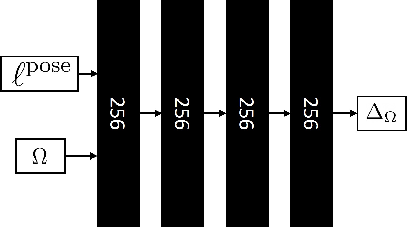
Fig. 7 and Fig. 8 show the network design of our canonical MLP and pose correction MLP. Specifically, we provide the details of how we incorporate appearance embedding $\ell^{\rm app}$ as well as pose embedding $\ell^{\rm pose}$ vectors into the corresponding networks.

Figure 7: Canonical $\rm MLP$ netwrok. We use an 8-layer MLP with width=256 that takes as input positional encoding $\gamma$ of position $\mathbf{x}$ and appearance embedding vector $\ell^{\rm app}$ with dimension=256. The network outputs color $\mathbf{c}$ and density $\mathbf{\sigma}$, following the design of NeRF [32]. There is a skip connection that concatenates $\gamma(\mathbf{x})$ to the fifth layer. We use ReLU activations after each fully connected layer. For the output layer, we use a ReLU activation for the density value $\mathbf{\sigma}$ to ensure non-negativity and a sigmoid activation for the color $\mathbf{c}$ to constrain values between 0 and 1.

Figure 8: Pose correction $\rm MLP$ network. We use a 4-layer MLP with width=256 that takes as input joint angles $\Omega$ and a pose embedding vector $\ell^{\rm pose}$ with dimension=16. The network produces the residuals of joint angles that are added back to the input pose to refine the body pose prediction.

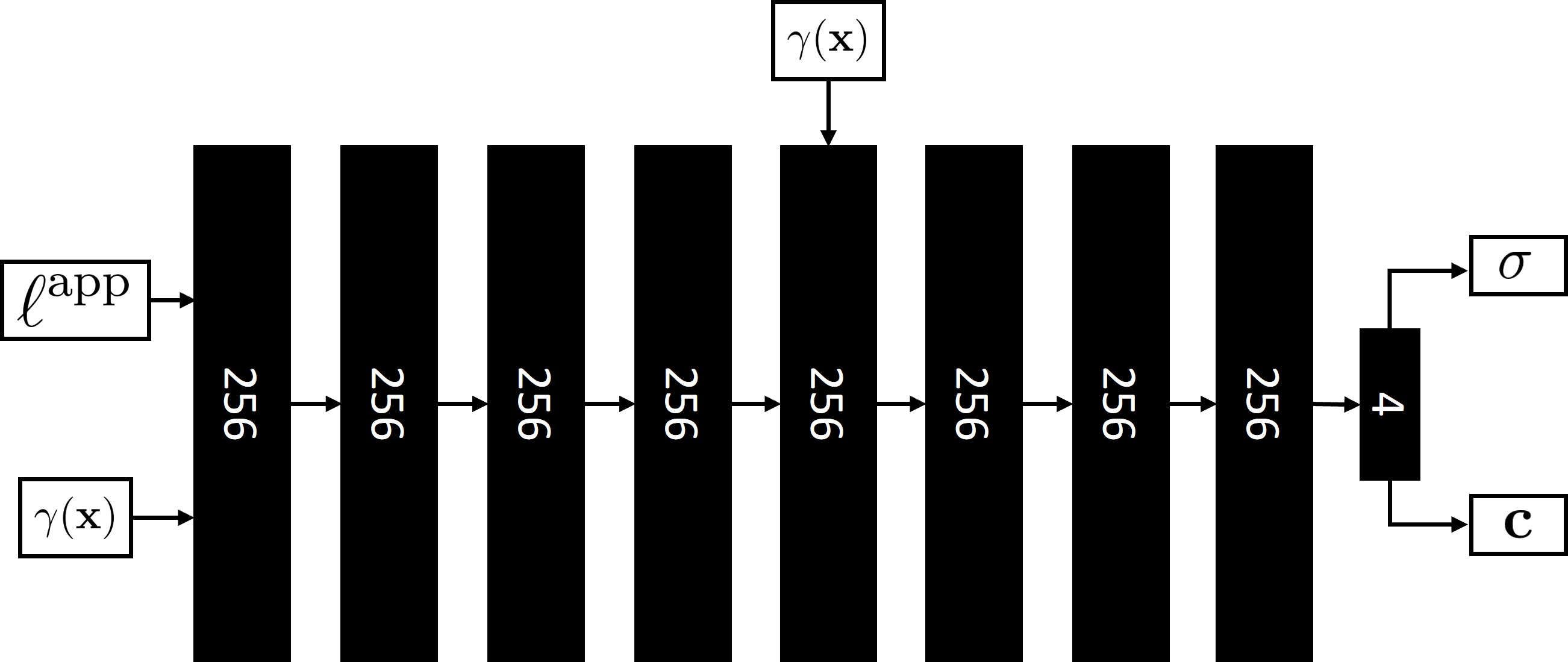
Appendix B Additional Results

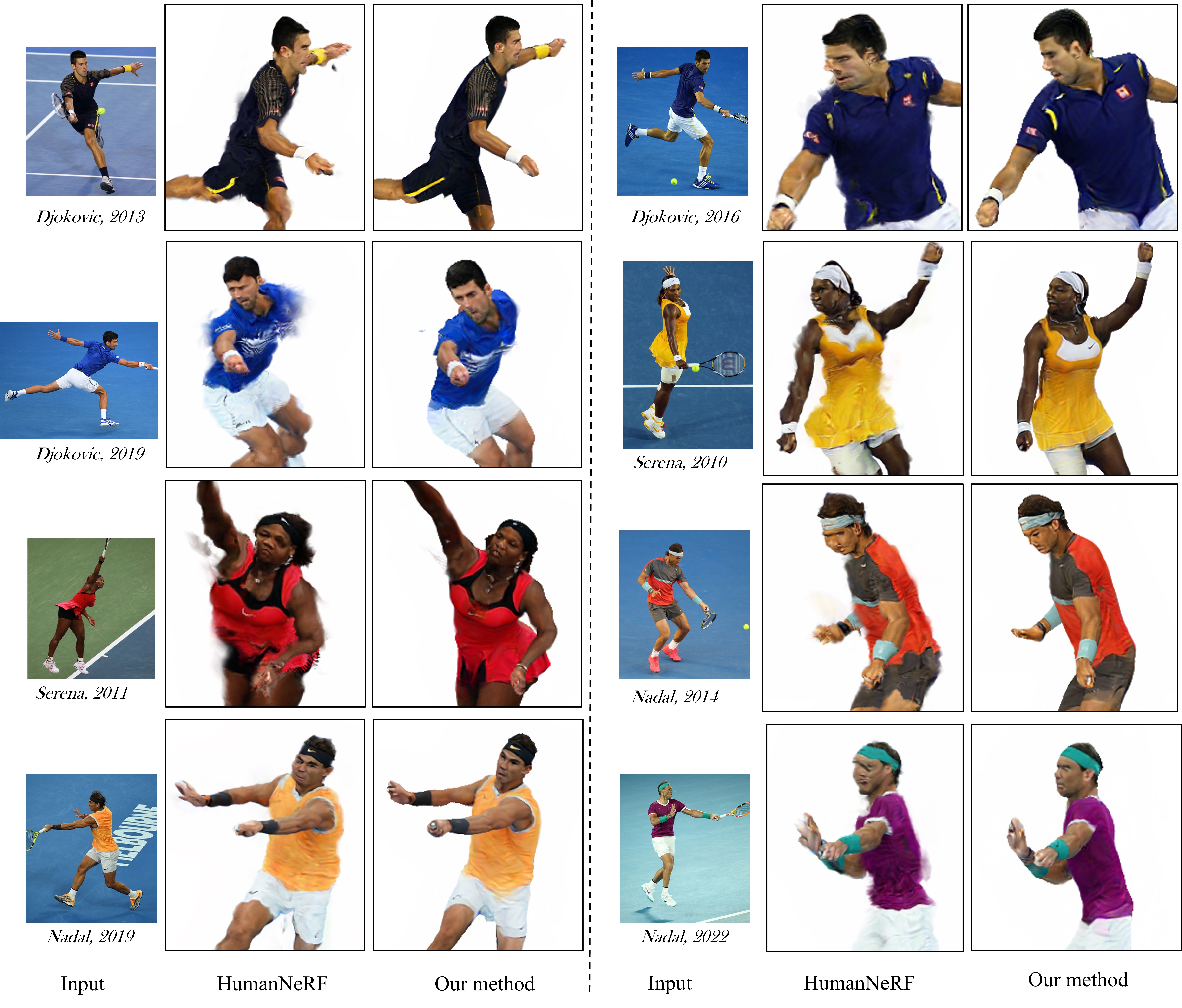
In addition to Roger Federer, we demonstrate our method on a wide variety of subjects that cover different genders and skin tones. In particular, we show results on three tennis athletes, Novak Djokovic, Serena Williams, and Rafael Nadal where each has three appearance sets in the datasets we collected. We present quantitative results in FID in Table 3 and visually compare them with HumanNeRF [46] in Fig. 9. The quality improvement over the related work is similar to the case of Roger Federer.

	Novak Djokovic			Serena Willams			Rafael Nadal
	2013	2016	2019	2009	2010	2011	2014	2019	2022
HumanNeRF [46]	87.07	62.01	64.17	104.23	100.52	113.41	90.04	64.95	76.68
Our method	81.38	57.14	58.74	87.81	90.70	85.17	80.95	62.75	61.71

Table 3: Comparison to related work: FID is computed per subject per year. Lower FID score is better.

Figure 9: Visual comparisons to HumanNeRF [46] on Novak Djokovic, Serena Willams, and Rafael Nadal. Photo credits to Getty Images.

Appendix C More Visualizations of Personalized Space

In the paper, we show a visualization of (appearance, camera view) plane of the reconstructed space of Roger Federer. Here we show the other two planes, (appearance, body pose) plane in Fig. 10 and (body pose, camera view) plane in Fig. 11 where we keep the camera view and appearance fixed, respectively.

Additionally, we show visualizations of the rebuilt personalized spaces of the other 3 persons, Novak Djokovic in Fig. 12, 13 and 14, Serena Willams in Fig. 15, 16 and 17, and Rafael Nadal in Fig. 18, 19 and 20.

Figure 10: Visualization of the (appearance, body pose) plane of the reconstructed space of Roger Federer.

Figure 11: Visualization of the (body pose, camera view) plane of the reconstructed space of Roger Federer.

Figure 12: Visualization of the (appearance, camera view) plane of the reconstructed space of Novak Djokovic.

Figure 13: Visualization of the (appearance, body pose) plane of the reconstructed space of Novak Djokovic.

Figure 14: Visualization of the (body pose, camera view) plane of the reconstructed space of Novak Djokovic.

Figure 15: Visualization of the (appearance, camera view) plane of the reconstructed space of Serena Willaims.

Figure 16: Visualization of the (appearance, body pose) plane of the reconstructed space of Serena Williams.

Figure 17: Visualization of the (body pose, camera view) plane of the reconstructed space of Serena Willaims.

Figure 18: Visualization of the (appearance, camera view) plane of the reconstructed space of Rafael Nadal.

Figure 19: Visualization of the (appearance, body pose) plane of the reconstructed space of Rafael Nadal.

Figure 20: Visualization of the (body pose, camera view) plane of the reconstructed space of Rafael Nadal.

References

- [1] Sameer Agarwal, Yasutaka Furukawa, Noah Snavely, Ian Simon, Brian Curless, Steven M Seitz, and Richard Szeliski. Building rome in a day. Communications of the ACM, 54(10):105–112, 2011.
- [2] Piotr Bojanowski, Armand Joulin, David Lopez-Paz, and Arthur Szlam. Optimizing the latent space of generative networks. arXiv preprint arXiv:1707.05776, 2017.
- [3] Joel Carranza, Christian Theobalt, Marcus A Magnor, and Hans-Peter Seidel. Free-viewpoint video of human actors. ACM transactions on graphics (TOG), 22(3):569–577, 2003.
- [4] Xu Chen, Yufeng Zheng, Michael J Black, Otmar Hilliges, and Andreas Geiger. Snarf: Differentiable forward skinning for animating non-rigid neural implicit shapes. In Proceedings of the IEEE/CVF International Conference on Computer Vision, pages 11594–11604, 2021.
- [5] Alvaro Collet, Ming Chuang, Pat Sweeney, Don Gillett, Dennis Evseev, David Calabrese, Hugues Hoppe, Adam Kirk, and Steve Sullivan. High-quality streamable free-viewpoint video. ACM Transactions on Graphics (ToG), 34(4):1–13, 2015.
- [6] Brian Curless and Marc Levoy. A volumetric method for building complex models from range images. In Proceedings of the 23rd annual conference on Computer graphics and interactive techniques, pages 303–312, 1996.
- [7] Paul E Debevec, Camillo J Taylor, and Jitendra Malik. Modeling and rendering architecture from photographs: A hybrid geometry-and image-based approach. In Proceedings of the 23rd annual conference on Computer graphics and interactive techniques, pages 11–20, 1996.
- [8] Zijian Dong, Chen Guo, Jie Song, Xu Chen, Andreas Geiger, and Otmar Hilliges. Pina: Learning a personalized implicit neural avatar from a single rgb-d video sequence. In Proceedings of the IEEE/CVF Conference on Computer Vision and Pattern Recognition, pages 20470–20480, 2022.
- [9] Mingsong Dou, Sameh Khamis, Yury Degtyarev, Philip Davidson, Sean Ryan Fanello, Adarsh Kowdle, Sergio Orts Escolano, Christoph Rhemann, David Kim, Jonathan Taylor, et al. Fusion4d: Real-time performance capture of challenging scenes. ACM Transactions on Graphics (ToG), 35(4):1–13, 2016.
- [10] Yasutaka Furukawa, Carlos Hernández, et al. Multi-view stereo: A tutorial. Foundations and Trends in Computer Graphics and Vision, 9(1-2):1–148, 2015.
- [11] Kaiwen Guo, Peter Lincoln, Philip Davidson, Jay Busch, Xueming Yu, Matt Whalen, Geoff Harvey, Sergio Orts-Escolano, Rohit Pandey, Jason Dourgarian, et al. The relightables: Volumetric performance capture of humans with realistic relighting. ACM Transactions on Graphics (ToG), 38(6):1–19, 2019.
- [12] Martin Heusel, Hubert Ramsauer, Thomas Unterthiner, Bernhard Nessler, and Sepp Hochreiter. Gans trained by a two time-scale update rule converge to a local nash equilibrium. Advances in neural information processing systems, 30, 2017.
- [13] Wei Jiang, Kwang Moo Yi, Golnoosh Samei, Oncel Tuzel, and Anurag Ranjan. Neuman: Neural human radiance field from a single video. arXiv preprint arXiv:2203.12575, 2022.
- [14] Takeo Kanade, Peter Rander, and PJ Narayanan. Virtualized reality: Constructing virtual worlds from real scenes. IEEE multimedia, 4(1):34–47, 1997.
- [15] Ira Kemelmacher-Shlizerman. Internet based morphable model. In Proceedings of the IEEE International Conference on Computer Vision (ICCV), December 2013.
- [16] Diederik P Kingma and Jimmy Ba. Adam: A method for stochastic optimization. arXiv preprint arXiv:1412.6980, 2014.
- [17] Nikos Kolotouros, Georgios Pavlakos, Michael J Black, and Kostas Daniilidis. Learning to reconstruct 3d human pose and shape via model-fitting in the loop. In ICCV, 2019.
- [18] Ruilong Li, Julian Tanke, Minh Vo, Michael Zollhofer, Jurgen Gall, Angjoo Kanazawa, and Christoph Lassner. Tava: Template-free animatable volumetric actors. arXiv preprint arXiv:2206.08929, 2022.
- [19] Zhengqi Li, Wenqi Xian, Abe Davis, and Noah Snavely. Crowdsampling the plenoptic function. In European Conference on Computer Vision, pages 178–196. Springer, 2020.
- [20] Shu Liang, Linda G Shapiro, and Ira Kemelmacher-Shlizerman. Head reconstruction from internet photos. In European Conference on Computer Vision, pages 360–374. Springer, 2016.
- [21] Lingjie Liu, Marc Habermann, Viktor Rudnev, Kripasindhu Sarkar, Jiatao Gu, and Christian Theobalt. Neural actor: Neural free-view synthesis of human actors with pose control. ACM Transactions on Graphics (TOG), 40(6):1–16, 2021.
- [22] Stephen Lombardi, Tomas Simon, Jason Saragih, Gabriel Schwartz, Andreas Lehrmann, and Yaser Sheikh. Neural volumes: Learning dynamic renderable volumes from images. SIGGRAPH, 2019.
- [23] Qianli Ma, Shunsuke Saito, Jinlong Yang, Siyu Tang, and Michael J Black. Scale: Modeling clothed humans with a surface codec of articulated local elements. In Proceedings of the IEEE/CVF Conference on Computer Vision and Pattern Recognition, pages 16082–16093, 2021.
- [24] Ricardo Martin-Brualla, David Gallup, and Steven M Seitz. 3d time-lapse reconstruction from internet photos. In Proceedings of the IEEE International Conference on Computer Vision, pages 1332–1340, 2015.
- [25] Ricardo Martin-Brualla, David Gallup, and Steven M Seitz. Time-lapse mining from internet photos. ACM Transactions on Graphics (TOG), 34(4):1–8, 2015.
- [26] Ricardo Martin-Brualla, Rohit Pandey, Shuoran Yang, Pavel Pidlypenskyi, Jonathan Taylor, Julien Valentin, Sameh Khamis, Philip Davidson, Anastasia Tkach, Peter Lincoln, et al. Lookingood: Enhancing performance capture with real-time neural re-rendering. arXiv preprint arXiv:1811.05029, 2018.
- [27] Ricardo Martin-Brualla, Noha Radwan, Mehdi S. M. Sajjadi, Jonathan T. Barron, Alexey Dosovitskiy, and Daniel Duckworth. NeRF in the Wild: Neural Radiance Fields for Unconstrained Photo Collections. In CVPR, 2021.
- [28] Wojciech Matusik, Chris Buehler, Ramesh Raskar, Steven J Gortler, and Leonard McMillan. Image-based visual hulls. In Proceedings of the 27th annual conference on Computer graphics and interactive techniques, pages 369–374, 2000.
- [29] Kevin Matzen and Noah Snavely. Scene chronology. In European conference on computer vision, pages 615–630. Springer, 2014.
- [30] Moustafa Meshry, Dan B Goldman, Sameh Khamis, Hugues Hoppe, Rohit Pandey, Noah Snavely, and Ricardo Martin-Brualla. Neural rerendering in the wild. In Proceedings of the IEEE/CVF Conference on Computer Vision and Pattern Recognition, pages 6878–6887, 2019.
- [31] Marko Mihajlovic, Yan Zhang, Michael J Black, and Siyu Tang. Leap: Learning articulated occupancy of people. In Proceedings of the IEEE/CVF Conference on Computer Vision and Pattern Recognition, pages 10461–10471, 2021.
- [32] Ben Mildenhall, Pratul P. Srinivasan, Matthew Tancik, Jonathan T. Barron, Ravi Ramamoorthi, and Ren Ng. NeRF: Representing scenes as neural radiance fields for view synthesis. ECCV, 2020.
- [33] Michael Niemeyer, Jonathan T. Barron, Ben Mildenhall, Mehdi S. M. Sajjadi, Andreas Geiger, and Noha Radwan. Regnerf: Regularizing neural radiance fields for view synthesis from sparse inputs. In Proc. IEEE Conf. on Computer Vision and Pattern Recognition (CVPR), 2022.
- [34] Sida Peng, Yuanqing Zhang, Yinghao Xu, Qianqian Wang, Qing Shuai, Hujun Bao, and Xiaowei Zhou. Neural body: Implicit neural representations with structured latent codes for novel view synthesis of dynamic humans. In Proceedings of the IEEE/CVF Conference on Computer Vision and Pattern Recognition, pages 9054–9063, 2021.
- [35] Shunsuke Saito, Jinlong Yang, Qianli Ma, and Michael J Black. Scanimate: Weakly supervised learning of skinned clothed avatar networks. In Proceedings of the IEEE/CVF Conference on Computer Vision and Pattern Recognition, pages 2886–2897, 2021.
- [36] Johannes L Schonberger and Jan-Michael Frahm. Structure-from-motion revisited. In Proceedings of the IEEE conference on computer vision and pattern recognition, pages 4104–4113, 2016.
- [37] Steven M Seitz, Brian Curless, James Diebel, Daniel Scharstein, and Richard Szeliski. A comparison and evaluation of multi-view stereo reconstruction algorithms. In 2006 IEEE computer society conference on computer vision and pattern recognition (CVPR’06), volume 1, pages 519–528. IEEE, 2006.
- [38] Qi Shan, Riley Adams, Brian Curless, Yasutaka Furukawa, and Steven M Seitz. The visual turing test for scene reconstruction. In 2013 International Conference on 3D Vision-3DV 2013, pages 25–32. IEEE, 2013.
- [39] Noah Snavely, Steven M. Seitz, and Richard Szeliski. Photo tourism: exploring photo collections in 3d. ACM Trans. Graph., 25(3):835–846, 2006.
- [40] Jiaming Sun, Xi Chen, Qianqian Wang, Zhengqi Li, Hadar Averbuch-Elor, Xiaowei Zhou, and Noah Snavely. Neural 3d reconstruction in the wild. In ACM SIGGRAPH 2022 Conference Proceedings, pages 1–9, 2022.
- [41] Richard Szeliski. Computer vision: algorithms and applications. Springer Nature, 2022.
- [42] Matthew Tancik, Vincent Casser, Xinchen Yan, Sabeek Pradhan, Ben Mildenhall, Pratul P Srinivasan, Jonathan T Barron, and Henrik Kretzschmar. Block-nerf: Scalable large scene neural view synthesis. In Proceedings of the IEEE/CVF Conference on Computer Vision and Pattern Recognition, pages 8248–8258, 2022.
- [43] Ayush Tewari, Ohad Fried, Justus Thies, Vincent Sitzmann, Stephen Lombardi, Kalyan Sunkavalli, Ricardo Martin-Brualla, Tomas Simon, Jason Saragih, Matthias Nießner, et al. State of the art on neural rendering. In Computer Graphics Forum, volume 39, pages 701–727. Wiley Online Library, 2020.
- [44] Ayush Tewari, Justus Thies, Ben Mildenhall, Pratul Srinivasan, Edgar Tretschk, W Yifan, Christoph Lassner, Vincent Sitzmann, Ricardo Martin-Brualla, Stephen Lombardi, et al. Advances in neural rendering. In Computer Graphics Forum, volume 41, pages 703–735. Wiley Online Library, 2022.
- [45] Garvita Tiwari, Nikolaos Sarafianos, Tony Tung, and Gerard Pons-Moll. Neural-gif: Neural generalized implicit functions for animating people in clothing. In Proceedings of the IEEE/CVF International Conference on Computer Vision, pages 11708–11718, 2021.
- [46] Chung-Yi Weng, Brian Curless, Pratul P. Srinivasan, Jonathan T. Barron, and Ira Kemelmacher-Shlizerman. HumanNeRF: Free-viewpoint rendering of moving people from monocular video. In Proceedings of the IEEE/CVF Conference on Computer Vision and Pattern Recognition (CVPR), pages 16210–16220, June 2022.
- [47] Yiheng Xie, Towaki Takikawa, Shunsuke Saito, Or Litany, Shiqin Yan, Numair Khan, Federico Tombari, James Tompkin, Vincent Sitzmann, and Srinath Sridhar. Neural fields in visual computing and beyond. Computer Graphics Forum, 2022.
- [48] Richard Zhang, Phillip Isola, Alexei A Efros, Eli Shechtman, and Oliver Wang. The unreasonable effectiveness of deep features as a perceptual metric. CVPR, 2018.
- [49] C Lawrence Zitnick, Sing Bing Kang, Matthew Uyttendaele, Simon Winder, and Richard Szeliski. High-quality video view interpolation using a layered representation. ACM transactions on graphics (TOG), 23(3):600–608, 2004.