Tensorial parametric model order reduction of nonlinear dynamical systems
Abstract
For a nonlinear dynamical system that depends on parameters, the paper introduces a novel tensorial reduced-order model (TROM). The reduced model is projection-based, and for systems with no parameters involved, it resembles proper orthogonal decomposition (POD) combined with the discrete empirical interpolation method (DEIM). For parametric systems, TROM employs low-rank tensor approximations in place of truncated SVD, a key dimension-reduction technique in POD with DEIM. Three popular low-rank tensor compression formats are considered for this purpose: canonical polyadic, Tucker, and tensor train. The use of multilinear algebra tools allows the incorporation of information about the parameter dependence of the system into the reduced model and leads to a POD-DEIM type ROM that (i) is parameter-specific (localized) and predicts the system dynamics for out-of-training set (unseen) parameter values, (ii) mitigates the adverse effects of high parameter space dimension, (iii) has online computational costs that depend only on tensor compression ranks but not on the full-order model size, and (iv) achieves lower reduced space dimensions compared to the conventional POD-DEIM ROM. The paper explains the method, analyzes its prediction power, and assesses its performance for two specific parameter-dependent nonlinear dynamical systems.
keywords:
Model order reduction, parametric dynamical systems, low-rank tensor approximations, proper orthogonal decomposition, discrete empirical interpolation method1 Introduction
The numerical solution of parametric dynamical systems is a common problem in areas such as numerical optimal control, shape optimization, inverse modeling, and uncertainty quantification. If the system is described by a set of evolutionary nonlinear partial differential equations (PDEs), then a straightforward approach that involves repeatedly solving a fully resolved discrete model for various parameter values can result in overwhelming computational costs. Reduced-order models (ROMs) offer a possibility to alleviate these costs by replacing the fully resolved model, also referred to as the full-order model (FOM), with a low-dimensional surrogate model [3, 18].
Reduced-order modeling for parametric dynamical systems has already attracted considerable attention, as seen in works such as [8, 21, 11, 4, 7, 10]. This paper contributes to the topic with a novel projection-based ROM that extends the ideas of proper orthogonal decomposition (POD) and discrete empirical interpolation method (DEIM) ROMs [31, 39, 13] to parametric systems using concepts and tools from tensor algebra. We refer to this approach as ’tensorial reduced-order modeling’ (TROM).
In general, a projection-based ROM constructs the surrogate model by projecting the high-fidelity FOM onto a low-dimensional problem-dependent vector space [8]. This space is computed from information provided by FOM solutions sampled at specific time instances and parameter values, often referred to as solution snapshots. When dealing with multiple and varying parameters, it can be challenging, or even impossible, to build a universal low-dimensional space that adequately represents solutions for all times and parameters of interest while still achieving sufficient order reduction. TROM addresses this problem by using a ’low-rank tensor decomposition’ (LRTD) in place of truncated singular value decomposition (SVD), a key dimension-reduction technique in both POD and DEIM. Similar to SVD, LRTD provides an orthogonal basis for a ’universal’ reduced-order space that can be sufficiently large to approximate the space of all observed snapshots. However, tensor low-rank representations also preserve information about the parameter dependence in this universal space, something that SVD/POD fail to offer. For any incoming parameter value, not necessarily from the training set, TROM uses this additional information to find a ’parameter-specific’ local reduced space, which is a low-dimensional subspace of the universal ROM space.
According to the outline above, dimension reduction in TROM is a two-stage process. In the first, ’offline’ stage, two approximate LRTDs are computed: one for the tensor of solution snapshots and another for the tensor of snapshots of the nonlinear term of the dynamical system. The second LRTD is required for a hyper-reduction DEIM-type method. The system is then projected onto the universal space provided by the first LRTD, and DEIM is performed using the universal space of the second LRTD. The resulting significantly reduced but still relatively large projected system is then passed to the next stage along with certain information about both LRTDs needed to compute the local reduced bases. In the second, ’online’ stage, for a given incoming vector of parameters, TROM computes bases for the local parameter-specific subspaces. These orthogonal bases are represented by their coordinates in the universal spaces. This allows for easy projection of the system onto the local reduced subspace and for performing a second (local) step of hyper-reduction. As demonstrated below, computation of local reduced bases and projection onto the local subspaces during the online stage involves operations only with low-dimensional matrices and vectors, making it fast. The distinguishing features of TROM are as follows: (i) it finds ’parameter-specific’ (local) reduced spaces during the online stage; (ii) the additional online costs are small and depend only on tensor ranks, not on the FOM resolution; (iii) depending on the low-rank tensor compression format used, the adverse effects of parameter space dimension can be mitigated; and (iv) reduced space dimensions are lower compared to the traditional POD–DEIM ROM for the same or better accuracy.
The concept of tensorial ROM was introduced recently in [32]. That paper explained the computation of universal and local projection spaces for three popular low-rank tensor formats (canonical polyadic, Tucker, and tensor train) and applied the method to two parameterized linear systems. This paper extends TROM for reduced-order modeling of nonlinear systems, which requires the application of a hyper-reduction technique, and introduces the concept of a tensor two-stage DEIM. We show that finding a local parameter-dependent representation of the nonlinear terms can be done in two stages, including LRTD in the offline stage and low-dimensional computations in the online stage. We provide an interpolation estimate for tensorial DEIM in terms of tensor decomposition accuracy, interpolation bounds in the parameter domain, and singular values of some local matrices.
The literature on tensor methods in reduced-order modeling of dynamical systems is rather limited. In addition to [32], we mention two papers [33, 34] that review tensor compressed formats and discuss their possible use for sparse function representation and reduced-order modeling, as well as a series of publications on the tensorization of algebraic systems resulting from the stochastic and parametric Galerkin finite element method, see, e.g., [9, 5, 6, 28, 27]. In [23], a POD-ROM was combined with an LRTD of a mapping from parameter space onto an output domain. Different approaches to making projection-based ROMs parameter-specific can be found in [17, 16, 2, 1, 40].
The rest of the paper is organized into six sections. Section 2 sets up the problem of interest. Section 3 summarizes the standard POD-DEIM ROM. Section 4 introduces the necessary tensor algebra preliminaries and reviews the concept of tensor rank. Section 5 explains TROM. Section 6 addresses the analysis of TROM, including the representation capacity of local reduced spaces and the interpolation property of tensorial DEIM. Finally, Section 7 assesses the performance of TROM for two examples of parameterized dynamical systems and compares it to that of the standard POD–DEIM ROM.
Notation conventions. The TROM and its analysis involve vectors, matrices, and tensors tailored to the full model, the reduced model, and some intermediate constructions. To assist the reader in navigating through the paper, we follow several notation conventions:we use lowercase letters for scalars, bold lowercase letters for vectors, upright capital letters for matrices, and all tensors will be denoted with bold uppercase letters (e.g. is a scalar, is a vector, is a matrix, and would be a tensor). For dimensions associated with the full-order model, we use uppercase Latin letters like , , , , and so on. To denote low-rank approximations of full-order tensors and related quantities, we use the tilde symbol ( ). For example, if is a full-order tensor, then represents its low-rank approximation. We may also use , , or , and so forth to denote tensor ranks. Vector spaces are denoted by uppercase Latin letters such as , , , and so on (Note: These should not be confused with upright capitals , , used for matrices). We reserve the letter ’n’ to represent the final reduced dimension of a ROM. When it’s necessary to distinguish between the final reduced dimensions of the ROM projection and DEIM interpolation spaces, we use and , respectively.
2 Problem formulation
The TROM framework we develop applies to steady-state and evolutionary systems arising from PDEs depending on parameters. We formulate the problem in the form of a general non-linear dynamical system. Specifically, for a given from the parameter domain , find the trajectory solving
| (1) |
with parameter dependent matrix , continuous flow field , and an initial condition . We assume that the unique solution exists on for all .
One can think about (1) as a system of ODEs resulting from a spatial discretization of a (nonlinear) parabolic problem, where the coefficients, boundary conditions, or the computational domain (through a mapping into a reference domain) are parameterized by .
Our focus is on a projection-based ROM, where, for any given , we seek an approximation to by solving a lower-dimensional system of equations obtained by projecting (1) onto a reduced space, known as the ROM space. For effective order reduction, it is essential that the ROM space is both problem-dependent and specific to .
Among the projection-based approaches for model reduction in time-dependent differential equations, one of the most common techniques is proper orthogonal decomposition enhanced with the discrete empirical interpolation method (POD–DEIM) to handle nonlinear terms [24, 37, 29, 30]. We provide an outline of the POD–DEIM ROM below for reference and for the purpose of comparison in Section 7. Additionally, reviewing the POD–DEIM ROM is instructive since the Tensorial Reduced Order Modeling (TROM) can be viewed as a natural extension of POD–DEIM to parametric problems.
3 Model reduction via POD–DEIM
Here we recap the conventional POD–DEIM ROM for non-linear systems adapted for the parametric case. Consider a training set of parameters sampled from the parameter domain, . Hereafter we use hats to denote parameters from the training set . At the first, offline stage of POD–DEIM, one computes through FOM numerical simulations a collection of solution snapshots
| (2) |
and non-linear term snapshots
| (3) |
further referred to as - and -snapshots, respectively, at times , and for from the training set . For a desired reduced space dimension , one computes the reduced space basis , referred to as the POD basis, such that the projection subspace approximates the space spanned by all -snapshots in the best possible way. This is achieved by assembling the matrix of all -snapshots
| (4) |
and computing its SVD
| (5) |
Then, the POD reduced basis vectors , , are taken to be the first left singular vectors of , i.e., the first columns of or in Matlab notation .
At the second, online stage, the POD–ROM solution is found through its vector of coordinates in the space , i.e., , which solve the projected system
| (6) |
While the pre-computation of the projected matrix during the offline stage enables fast matrix-vector multiplications for evaluating (6), efficiently evaluating the nonlinear term in (6) during the online stage is generally challenging. The discrete empirical interpolation method (DEIM) addresses this challenge effectively. In this widely-used hyper-reduction technique, the nonlinear term is approximated within a lower-dimensional subspace of , the space spanned by all FOM -snapshots. SVD is employed to find the basis for this subspace, where represents the -th left singular vector of the matrix:
| (7) |
comprising all -snapshots. To ease notation, also take first left singular vectors of (7) to form . For stability and accuracy considerations, it’s possible for and to contain different numbers of vectors. In such cases, we refer to these dimensions as and , respectively. We refer to as the POD–DEIM reduced -space and the columns of as the POD–DEIM -reduced basis. Then, DEIM approximates the nonlinear term of (1) via
| (8) |
where the ’selection’ matrix is defined as:
| (9) |
This matrix, , is constructed so that for any , the vector contains entries selected from with indices . DEIM determines entirely based on the information within using a greedy algorithm, as detailed in [13].
The singular values of and provide information about the representation power of and , respectively. In particular, it holds:
| (10) |
for representation of the solution states, and similarly for and -snapshots .
Summarizing, the POD–DEIM ROM of (1) takes the form
| (11) |
with the initial condition , for so that is approximated by , where .
A key requirement for the efficient evaluation of the nonlinear term is that for a fixed and , an arbitrary given entry of vector can be computed quickly, with costs independent of dimensions and . To meet this requirement, we assume that each depends on a few entries of , i.e., , with independent on and .
Please note that the POD–DEIM reduced bases capture cumulative rather than localized information about the dependence of - and -snapshots on . Without this parameter-specificity, both bases may lack robustness for parameter values outside the training set, and this limitation can even apply to in-sample parameters if the reduced dimension is not sufficiently high. In other words, POD–DEIM bases might not perform well away from the reference FOM simulations. This poses a significant challenge when applying POD-based ROMs in tasks like inverse modeling. To address this challenge, we introduce tensor techniques with the aim to preserve the information about parameter dependence in lower dimensional spaces and next to benefit from it at the online stage. We continue with some preliminaries from multi-linear algebra.
4 Multi-linear algebra preliminaries and tensor decompositions
Assume that the parameter domain is the -dimensional box
| (12) |
Also, let the training set be a Cartesian grid: distribute nodes within each of the intervals in (12) for , and let
| (13) |
The cardinality of is obviously .
Given the structure (13) of the training set, the FOM solution - and -snapshots are naturally organized in the multi-dimensional arrays
| (14) |
which are tensors of order and size , i.e., , , . We reserve the first and last indices of , for dimensions corresponding to the spatial and temporal resolution, respectively.
Throughout the rest of this section, is a generic tensor of the same order and size as the - and -snapshots tensors. Unfolding of is reordering of its elements into a matrix. If all 1st-mode fibers of , i.e. all vectors , are organized into columns of a matrix, we get the 1st-mode unfolding matrix, denoted by . A particular ordering of the columns in is not important for the purposes of this paper. Thus, and are 1st-mode unfolding matrices of tensors and . We seek to replace the (truncated) SVDs of and with low-rank approximations of and directly in tensor format.
Unlike the matrix case, the notion of tensor rank is ambiguous. The problem of defining a tensor rank(s) has been extensively addressed in the literature; see e.g. [19]. For our purpose we choose three tensor formats which lead to different definitions of a rank and offer three compressed tensor representations or LRTD. These three formats: canonical polyadic (CP), Tucker (a.k.a high-order singular value decomposition, HOSVD), and tensor train (TT), are recalled below.
In the CP format [22, 12, 25, 26], one represents a tensor by the sum of outer products of vectors , , , and ,
| (15) |
Here is the so-called CP-rank and an outer product of vectors is defined as an rank one tensor with entries .
The HOSVD represents a tensor in the Tucker format [41, 26]:
| (16) |
with a core tensor and vectors , , and . The sizes of core tensor in all dimensions, i.e., , , , and , are referred to as Tucker ranks of .
Finally, the tensor train decomposition [36] represents a tensor in the TT-format:
| (17) |
with , , and , where the positive integers are referred to as the compression ranks (or TT-ranks) of the decomposition. For higher order tensors the TT format is in general more efficient compared to HOSVD. This may be beneficial for larger . Note that unlike CP or HOSVD formats, compression ranks of TT decomposition may depend on the order in which the snapshots are organized in tensors and . Throughout this paper we use the ordering as in (14). However, a different order may decrease the compression ranks further.
All three decompositions can be viewed as extensions of SVD to multi-dimensional arrays but having different numerical and compression properties. In particular, finding the best approximation of tensor by a fixed-ranks tensor in Tucker and TT format is a well-posed problem with constructive algorithms known to deliver quasi-optimal solutions [14, 36]. Furthermore, using these algorithms based on truncated SVD for a sequence of unfolding matrices, one may find (in Tucker or TT format) that satisfies
| (18) |
for given . Corresponding Tucker or TT ranks are then recovered in the course of factorization. Here and further, denotes the tensor Frobenius norm, which is simply the square root of the sum of the squares of all entries of .
The -mode tensor-vector product of a tensor of order and a vector is a tensor of order and size :
| (19) |
Analogously, the -mode tensor-matrix product of a tensor and a matrix is a tensor of order and size :
| (20) |
In what follows we assume that and are compressed representations of - and -snapshot tensors and , respectively, in one of the formats discussed above. To minimize notation burden, we assume they satisfy (18) with some which is the same for both and compression.
5 Tensorial ROM for nonlinear dynamical systems
5.1 Universal and local reduced spaces
Each of the two stages of the TROM algorithm is associated with distinct reduced spaces. The reduced spaces computed during the offline stage are referred to as the ’universal’ reduced spaces, while the ’local’ reduced spaces are employed in the online stage. We will describe both types of reduced spaces below.
Universal reduced spaces are the spans of all 1st-mode fibers of the compressed tensors, i.e.,
| (21) |
The dimension of is equal to the first Tucker or TT rank of (if Tucker or TT formats are used) and it does not exceed for the CP compression format. We also denote by and the matrices with columns that form orthonormal bases for and , respectively.
The universal spaces represent all observed - and -snapshots up to the tensor compression accuracy. Indeed, let , where , then it holds
| (22) |
where we used for a matrix and a tensor of compatible sizes, and spectral matrix norm . We also used for the orthogonal projection matrix .
The bound (22) and a similar bound for -snapshots resembles the POD optimal representation property (10). Universal spaces and can be seen as TROM counterparts of POD–DEIM ROM spaces and In fact, if SVD-based algorithms from [14, 36] are applied to find and in Tucker or TT-formats, then it holds and if and the same training set is used for both POD and TROM. The advantage of LRTD over POD is that and contain information about variation of - and -snapshots with respect to . This additional information enables us to find the subspaces of and referred to as local reduced spaces that are best suitable for the representation of and for any specific . These local reduced spaces are then used for online TROM’s stage. Their dimensions can be (much) lower than the dimensions of and , thus the universal spaces can be allowed to be sufficiently large (by choosing small enough) to accurately represent all - and -snapshots without any decrease of ROM performance at the online stage.
To define parameter-specific local reduced spaces for an arbitrary , we need an interpolation procedure in parameter domain
| (23) |
such that for a smooth function one approximates , where , and , , are the grid nodes on . In this paper we consider (23) corresponding to Lagrange interpolation of order : for a given let be the closest grid nodes to in , for , then
| (24) |
Lagrange interpolation is not the only possible option, of course.
With the help of (23) we introduce the local snapshot matrices and via the following “extraction–interpolation” procedure:
| (25) |
If is a parameter from the training set, then encodes the position of among the grid nodes on . Therefore, for the matrices , are exactly the matrices of all - and -snapshots for the particular (“extraction”). Otherwise, for a general matrices , are the result of interpolation between pre-computed snapshots.
Finally, we have all the required pieces to define the local spaces. For arbitrary given the parameter-specific local reduced -space of dimension is the space spanned by the first left singular vectors of , where . Similarly, the parameter-specific local reduced -space of dimension is spanned by the first left singular vectors of , . It is quite remarkable that orthogonal bases for each of these local spaces can be calculated quickly (i.e., using only low-dimensional calculations) through their coordinates in the corresponding universal spaces without assembling or explicitly. TROM framework performs this “on the fly” during the online stage for any incoming , as explained later.
In summary, the universal spaces, within a compression accuracy of , encompass the spaces
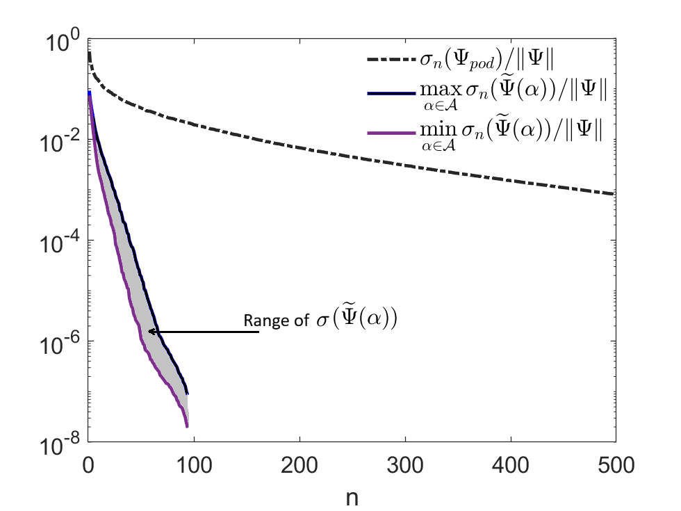
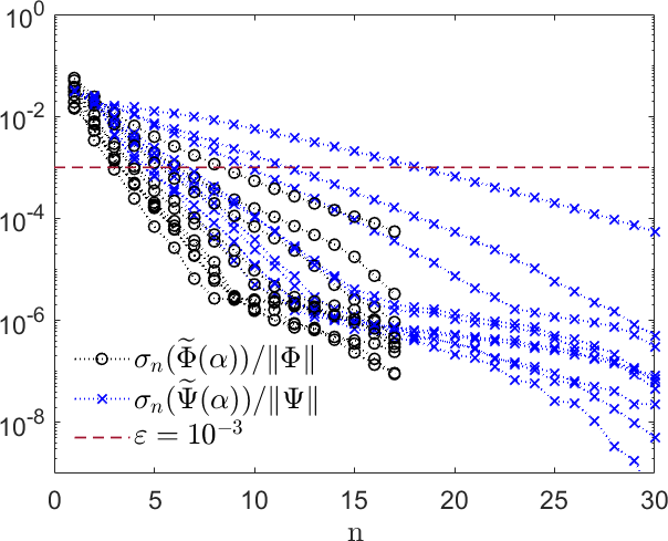
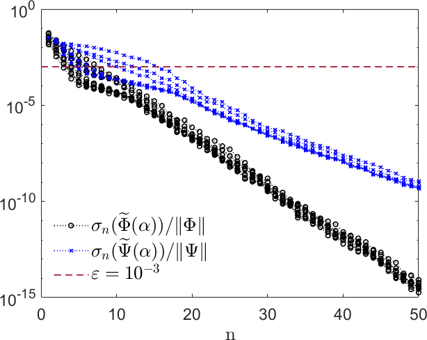
formed by all observed snapshots. These spaces resemble those utilized by the conventional POD-DEIM ROM, where the SVD of matrices containing all - and -snapshots is truncated based on the desired dimension or approximation accuracy. In the TROM framework, this truncated SVD is substituted with LRTD in one of the formats (15)–(17). Beyond the universal reduced spaces, the two-stage TROM framework also takes advantage of -specific ’subspaces’ within the universal spaces, known as the local reduced spaces. We illustrate the usefulness of local reduced spaces through a numerical example of the parametrized Allen-Cahn equations (for a complete problem description, see Section 7) in Figure 1. This figure compares the singular values of with the singular values of for a random sampling of . Truncation by and determines the representation power of the standard POD-DEIM ROM interpolation space and the TROM local space of a fixed dimension . We observe a significant enhancement in the representation power of TROM local spaces compared to POD-DEIM ROM spaces, demonstrating the benefits of taking into account information on -dependence during the offline decomposition stage.
5.2 Two-stage TROM-DEIM process
With all the preliminaries in order, we are now ready to introduce the two-stage process for computing tensorial reduced order model that incorporates DEIM to handle nonlinearity. One may formulate at least three variants of this process, each corresponding to the considered LRTD format. However, the main steps remain the same for all three variants. Therefore, we will present the TT version of the TROM-DEIM process, with additional comments regarding the necessary adjustments for other LRTD formats provided at the end of this section.
Offline stage. The first calculation is to compute TT decomposition to both -snapshot tensor and -snapshot tensor , satisfying (18):
| (26) |
with , , and . TT decompositions , may be found by using a stable algorithm based on truncated SVD for a sequence of unfolding matrices [36, 35] with computational costs similar to finding and for the conventional POD–DEIM ROM. We organize vectors from (26) into matrices
| (27) | ||||
| (28) |
where and are the first and last TT ranks of both snapshot tensors , respectively. We also consider third order tensors , defined entry-wise as
| (29) |
for all , for both snapshot tensors , respectively. While both and are orthogonal matrices, the columns of and are orthogonal, but not necessarily orthonormal. Thus, we need diagonal scaling matrices
Then, the essential information about the compressed TT representations that is transmitted to the online phase is assembled into
| (30) |
To perform hyper-reduction, DEIM algorithm is applied to the orthonormal columns of to compute the indices of the selection matrix . Then, the matrices
| (31) |
are computed and passed onto the online stage along with the TT cores (30).
If one or both terms and in (1) do not contain a dependence on the parameter, they can be projected for later use to save computation at the online stage:
Analogously, the projections can be pre-computed offline if the dependence on parameters is explicit of the form with some given functions and parameter-free matrices and similarly for .
Online stage. The second stage of the TROM process is specific for a particular incoming value of . In particular, it computes the two local reduced bases via their coordinates in the universal reduced bases, the columns of and , respectively. To achieve this, use the cores (30) to define the parameter-specific core matrices as the product
| (32) |
for . After rescaling with , take the SVD of the rescaled core matrices
| (33) |
which is computationally cheap since ’s and ’s have reduced dimensions. This allows one to obtain the SVD of the local snapshot matrices from (25) without explicitly assembling them. To see this, note the identities
| (34) |
and similar for . Since all matrices , , , , have orthonormal columns, the right-hand sides of (34) are the (thin) SVDs of and , respectively. Therefore, the coordinates of the local reduced -basis in the universal space are given by the first columns of . Similarly, the coordinates of the local reduced -basis in the universal space are the first columns of . We denote and . Thus the local projection and interpolation spaces are and .
After computing the coordinates of local reduced bases, an additional hyper-reduction step is performed. Below we introduce two variants of this local hyper-reduction procedure: (i) local DEIM and (ii) local least squares fitting.
(i) Local DEIM is done by applying DEIM algorithm to to obtain the indices and the corresponding selection matrix . Then, the non-linear term can be found using the matrices (31) precomputed at the offline stage:
| (35) |
(ii) Local LS fitting. Thanks to reduced dimensions of the universal and local space, it is computationally inexpensive to solve the fitting problem of finding such that in the least square sense. Then, the non-linear term representation takes the form
| (36) |
where denotes the pseudo-inverse of -matrix .
Along with either variant of local hyper-reduction, the pre-projected matrix is projected further to obtain
| (37) |
Finally, the TROM of (1) takes the form: Find solving
| (38) |
with the initial condition , so that is approximated by , where .
We summarize both stages described above in the Algorithm 1. In practice, one may pick different reduced dimensions for the local reduced - and -spaces. When we need to distinguish them, we use and , respectively.
- •
-
•
Online stage.
Input: decomposition cores (30), local reduced space dimensions(39) and an incoming parameter vector ;
Output: Coordinates of the local reduced bases in the form of matrices and ;
Compute:
After the model reduction is done according to Algorithm 1, the projected problem (38) is solved with either (35), (37) or (36), (37). One lets . For another incoming vector of parameters , the online part of Algorithm 1 should be recomputed.
Remark 1 (Computational complexity).
Let us introduce and . Then, the bulk of the computational cost of the online stage of TROM-DEIM is in the SVD computation (33) which takes . This is followed by integration of (38) costing . This compares favorably to POD-ROM integration cost of , provided which is always the case for reasonably long integration times. Then, the speed up of TROM–DEIM relative to POD–ROM is determined by the ratio of dimensions of local and universal spaces.
We conclude with a brief discussion of variants of Algorithm 1 based on the other two LRTD formats by pointing out the required modifications.
HOSVD-TROM. For Step 1 of the offline stage we employ HOSVD-LRTD (16) instead of TT-LRTD (17), so the cores (30) are replaced with
| (40) |
where , . The matrices and are still assembled as in (27)–(28), but the vectors , , and , come from HOSVD-LRTD (16) instead. At the online stage of Algorithm 1 the bound (39) is replaced by , , while the core matrices (32) at Step 1 are instead computed as
| (41) |
Unlike the TT case, no rescaling is needed for HOSVD core matrices (41), so the SVD in Step 2 of the online stage becomes simply
| (42) |
CP-TROM. For CP-TROM, the replacement of LRTD in Step 1 of the offline stage with (15) can be computed through two distinct approaches. Firstly, one can employ a Proper Generalized Decomposition method to compute CP-LRTD incrementally in a greedy manner, gradually increasing the CP-ranks and until the target accuracy is achieved [15]. Alternatively, the target ranks and can be specified initially, and an ALS algorithm can be used to compute CP-LRTD [26]. In this context, we opt for the latter approach due to the availability of high-performance ALS implementations.
For the matrices
| (43) | ||||
| (44) |
their thin QR factorizations are computed , , , , in order to obtain the cores
| (45) | |||||
| (46) |
6 Representation and interpolation estimates
In this section we consider representation capacity of TROM local reduced bases and prove an interpolation estimate for the two-stage TROM–DEIM. To do so, we need a few assumptions about the properties of the dynamical system (1). In particular, we assume that the unique solution to (1) exists on for all , with some and . Also, is continuous with continuous derivatives in and up to order :
| (49) |
where is interpolation order parameter from (24). For a vector function we define its norm as maximum over all components .
The assumption in (49) implies that the solution of (1) is smooth with respect to parameters. More precisely, it holds (cf. [20, Theorem V.4.1]):
| (50) |
Letting we apply the chain rule and use (50) to estimate
| (51) |
with some independent of FOM dimensions.
For an arbitrary fixed , not necessarily from the sampling set, consider the FOM -snapshots of (1) and the corresponding -snapshots,
Denote by , , the basis vectors of the local reduced -space, i.e., are the first left singular vectors of . This local basis used to represent TROM solution admits the following representation estimate [32]:
| (52) |
where are the singular values of and are the mesh parameter of the sampling,
| (53) |
Constants and in (52) depend only on the stability of the interpolation procedure and bounds on partial derivatives of from (50). The scaling accounts for the variation of dimensions and , which may correspond to the number of temporal and spatial degrees of freedom, if (1) results from a discretization of a parabolic PDE. In this case and for uniform grids, the quantity on the left-hand side of (52) is consistent with the norm.
We now want to derive an interpolation bound for the two-stage TROM–DEIM. For the POD–DEIM ROM such bound is given in the original paper [13]. In our notation the result reads: For some let , then it holds A bound on was also derived in [13]. Applying this result for in-sample , one finds the interpolation estimate
| (54) |
In the context of ROM for parametric systems, the estimate in (54) shows the following limitations: (i) It is not clear how it can be extended for an out-of-sample , and (ii) For the case of higher variability w.r.t. parameters, the singular values of may decrease relatively slowly (see Figure 1) requiring higher dimensions of reduced -spaces. The interpolation bound for the two-stage TROM–DEIM given below addresses both of the above issues.
Theorem 6.1.
For any given , let , for the local pointwise interpolation and for the least-square local interpolation. Also let , and are singular values of . It holds
| (55) |
with for the local pointwise interpolation and for the least-square local interpolation. Constants , are independent of , sampling grid, local TROM dimension , tensor ranks and FOM dimensions.
Proof 6.2.
Note that for the local DEIM the matrix is invertible and hence its inverse coincides with the pseudo-inverse, so we use the notation throughout the proof to cover both local hyper-reduction variants. Clearly, for both variants is the left inverse of and so we have the identity . We employ it to estimate
| (56) |
For the local DEIM, the first factor on the right-hand side of (56) can be estimated by the same argument as in [13]:
| (57) |
where the first identity holds since is a projector.
For the local LS fitting the matrix is still a projector. Furthermore, for any , where is the dimension of the universal reduced space , and , it holds , where is the orthogonal projector on the range of .
Let , then we have implying
This yields and so for the local LS fitting we have
| (58) |
Consider the SVD of from (25) given by
| (59) |
Then from the definition of the basis for the local reduced -space it follows that are the first columns of . Let , then
| (60) |
where we used triangle inequality and for the spectral norm of the projector. For the last term in (60), we observe
| (61) |
To handle the first term of (60), consider the interpolation of the full (non-compressed) -snapshot tensor , and proceed using the triangle inequality
| (62) |
The polynomial interpolation procedure is stable in the sense that
| (63) |
where is the column of the identity matrix, and with some independent of and (e.g., for linear interpolation). We use this and (18) to bound the second term of (62). Specifically,
| (64) |
It remains to handle the first term in (62). The choice of interpolation procedure in (24) implies that for any sufficiently smooth it holds
| (65) |
for , where the constant does not depend on .
Using the shortcut notation and interpolation property (65), we compute
where . The -term obeys a component-wise bound
where the absolute value of vectors is understood entry-wise. Analogously, we compute
| (66) |
with a component-wise bound for the remainder
Applying the same argument repeatedly, we obtain
| (67) |
with a component-wise bound for the remainder
Using the definition of the Frobenius norm and (67), we arrive at
| (68) |
with constants , , from (65), (63), and (51), respectively. Combining (56)–(58), (60)–(62), (64) and (68) proves the final result.
7 Numerical experiments
We perform several numerical experiments to assess the performance of the TROM and compare it to the POD–DEIM ROM. Our testing is performed for dynamical systems arising from discretizations of the parameter-dependent Burgers and Allen-Cahn equations. All results presented below are for the local least squares second stage of the hyper-reduction. The local DEIM as the second stage were found to yield very close results.
7.1 Parameterized 1D Burgers equation
As a first example consider the 1D Burgers equation: Find , solving
| (69) |
where is the viscosity parameter. The initial condition is in parametric form
| (70) |
Thus, we consider a two-parameter system, with the parameter domain .
We discretize (69)–(70) in space using a first order upwind finite difference (FD) scheme on a uniform grid with mesh size to obtain a dynamical system of the form (1), where depends on only and the non-linear term is the discretization of that does not contain any dependence on .
To generate FOM snapshots we integrate in (1) time using a semi-implicit BDF2 method with equidistant time stepping: for each , given and in , find satisfying
| (71) |
with first step performed via BDF1. Here , , , and . We denote by the matrix discretization of the first derivative, with boundary conditions (69). The operation denotes entrywise product of vectors in .
Once the time-stepping (71) is computed, -snapshots are given by
| (72) |
| 0.1 | 0.03 | 0.01 | 0.003 | ||
| TT-ranks | |||||
| TT-ranks | |||||
| 18824 | 4894 | 1518 | 536 | 270 | |
| 620 | 202 | 95 | 54 | 37 | |
| CP-rank | 50 | 100 | 200 | 300 | 500 |
| 8274 | 2749 | 822 | 391 | 149 |
7.1.1 Tensor compression accuracy and TROM solution quality
In the first series of experiments we study the performance of TROMs depending on the LRTD accuracy . We set , and use a rather fine grid of uniformly distributed values in , and values of log-uniformly distributed in to define the sampling set .
For TT-TROM we start with a low accuracy of (we always set the same target accuracy for and ) and gradually improve it letting . We report in Table 1 the resulting TT compression ranks in the format for both , and the compression factor
| (73) |
for , where is the number of entries of the full snapshot tensor and is the amount of data passed in Algorithm 1 from the offline stage to the online stage. For CP-TROM we used the combined compression factor
| (74) |
The first and last TT ranks emphasized in bold are responsible for the universal reduced space dimension and the maximum possible local reduced space dimension, respectively. For the same , the first and last Tucker ranks (not shown) of HOSVD-TROM were found to be the same as the first and last TT ranks, but the HOSVD-TROM compression factor (not shown) was slightly worse than those of TT-TROM. The higher TT ranks for than for indicate a higher variability in -snapshots compared to that of -snapshots. We shall see that this high variability results into a dramatic accuracy gain of TROMs compared to conventional POD–DEIM ROM.
| TT-TROM | CP-TROM |
|---|---|
 |
 |
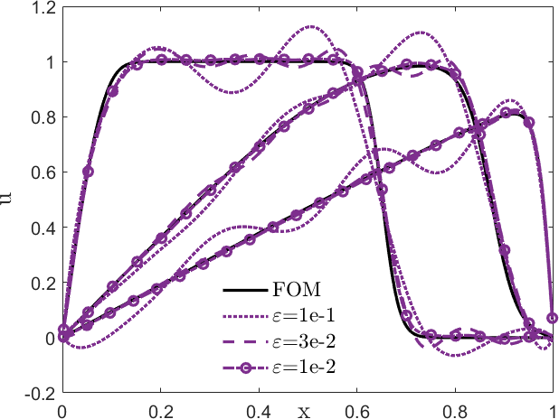
To assess the effect of tensor compression accuracy on the TROM solutions, we selected an out-of-sample parameter vector and computed the corresponding TT-TROM solution at . We set for , which corresponds to using the local reduced spaces of the largest possible dimension; see the bound in (39). The resulting solution is displayed in Figure 2 (left), where it is compared to the FOM solution. The HOSVD-TROM solutions were virtually identical to those provided by TT-TROM, so we do not display them separately. We observe that TT-TROM solutions for exhibit significant inaccuracies, but the results improve rapidly for smaller values of . For , the TT-TROM solutions closely align with the FOM solution. We do not present the TT-TROM solutions for since they are visually indistinguishable from the FOM solution.
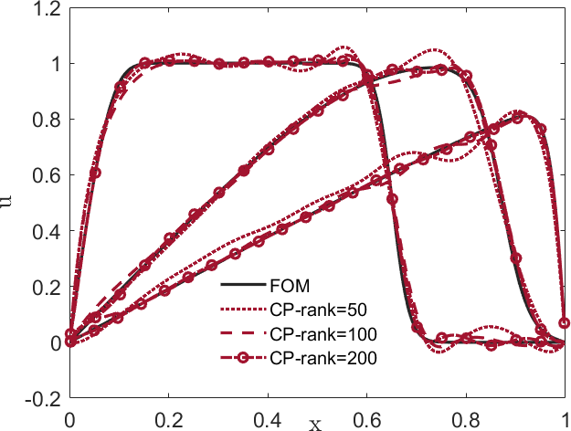
In Figure 2 (right), we present the results of a similar study for CP-TROM, where the CP-rank is predetermined instead of targeting a specific accuracy . The experiment covers CP-ranks of (further increasing the CP-rank leads to a very slow convergence of the ALS method [26] for computing CP LRTD). The corresponding compression accuracy of and is detailed in the lower part of Table 1.
We note that the best compression accuracy achieved by CP-TROM for is only (for CP-rank=). In Figure 2 (right), CP-TROM solutions are displayed for CP-ranks of and , with and . For CP-rank=, the dimensions of the local reduced spaces are chosen to be and . This choice of and aligns with the TT-TROM local reduced space dimensions of comparable compression accuracy.
| , | , |
 |
 |
| , | POD–DEIM ROM for |
 |
 |
7.1.2 Out-of-sample TROM performance
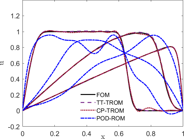
In this series of experiments we examine the performance of TROMs for out-of-sample parameter values depending on the dimensions of the local - and -spaces, denoted by and , respectively. We use the same sampling set as in Section 7.1.1 and the same out-of-sample parameter vextor . For both and tensors, we perform TT LRTD with and CP LRTD with CP-rank= resulting in CP approximation accuracy of and .
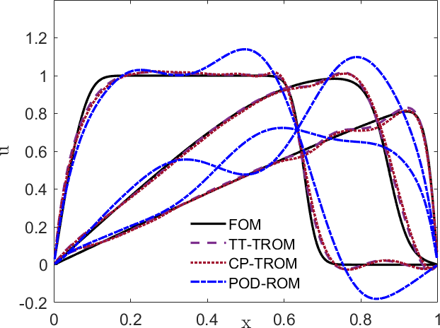
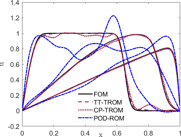
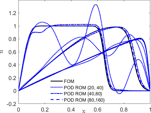
In Figure 3 we display both FOM and ROM solutions of the discretized Burgers equation at times , for increasing values of and . We observe that already for and both TT- and CP-TROM deliver reasonable approximations to the FOM solution. Increasing local reduced space dimensions to and , results in TROM solutions that almost match the FOM solutions. Remarkably, the further increase to and leads to CP-TROM solutions with some spurious oscillations, while TT-TROM solution provides a highly accurate approximation to the FOM solution. We attribute this degrade of CP-TROM to the failure of CP to approximate the snapshot tensors well for CP-rank= resulting in spurious higher order singular vectors in the bases and/or . We display in all plots in Figure 3 solutions obtained with the conventional POD–DEIM ROM approach for the same dimensions and . For all the dimensions considered POD–DEIM ROM fails to capture the behavior of the FOM solution. The right-bottom plot suggests that only for dimensions close to FOM size, it is possible for POD–DEIM ROM to ensure high quality of the solution, which defeats the purpose of model reduction.
 |
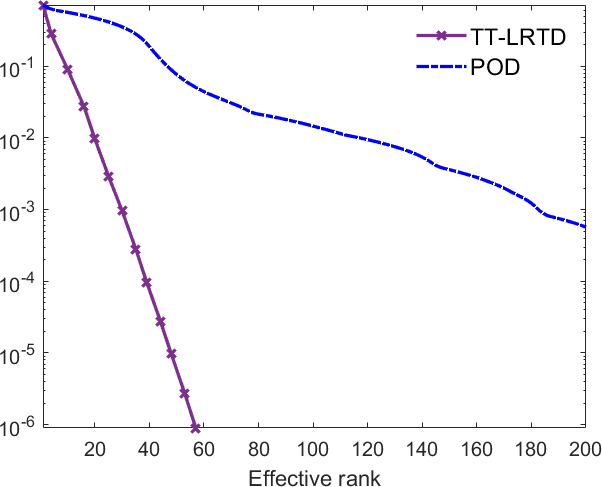 |
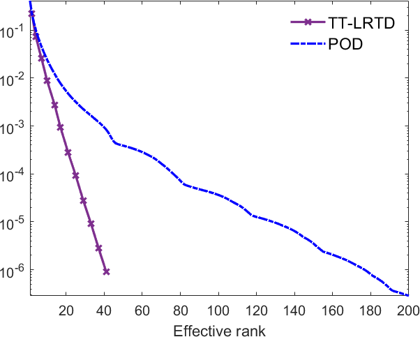
The dramatic gain in the ROM solution quality offered by the TROM compared to POD–DEIM ROM, as observed in Figure 3, can be understood by exploring the relative approximation error of LRTD versus POD in terms of their effective rank. The effective ranks for TT- and HOSVD-LRTD are defined as from (17) and from (16) respectively. For the truncated SVD of POD–DEIM ROM the effective rank is just the number of singular values/vectors kept in , .
For LRTD employed in TROM we define the relative approximation errors for the - and - snapshot tensors as
| (75) |
respectively. For the truncated SVD employed by POD–DEIM ROM the relative errors are
| (76) |
where are the 1-mode unfolding matrices of the snapshot tensors , and are their truncated SVDs for both . In practice, TT and HOSVD effective ranks are essentially the same, so we only report the errors (75) for TT-LRTD.
Figure 4 shows that for the same effective rank TT-LRTD provides a significantly smaller relative error compared to the truncated SVD for both - and -snapshot approximations. Moreover, the accuracy gain is especially pronounced for approximating -snapshots.
| TT-TROM | CP-TROM |
|---|---|
 |
 |
Results in Figure 3 suggest that TT-TROM solutions are reasonably accurate even for the local dimensions lower than those given by the last TT rank: , . This behavior is explained by the left plot in Figure 5, which shows the scaled singular values of the local snapshot matrices and for several random realizations of out-of-sample parameters . Note that and appear on the right-hand side of the TROM representation estimate (52) and DEIM interpolation estimate (55). While setting makes the corresponding terms in (52) and (55) vanish, for smaller (but not too small) local reduced space dimensions they are dominated by approximation terms and so do not affect the representation power of the local reduced spaces.
| 16x32 | 32x64 | ||||
|---|---|---|---|---|---|
| 0.244 | 0.104 | 0.035 | 0.025 | 0.026 | |
| 0.442 | 0.204 | 0.060 | 0.030 | 0.033 |
Finally we examine the dependence of TROM solution accuracy on the sampling refinement for the parameter space. Table 2 shows errors in the norm, which is a natural norm for parabolic problems. The error is averaged and maximal over 100 pairs of out-of-sample parameters randomly drawn. We see that the error decays with refining the parameter grid as predicted by the representation estimate with saturation achieved for .
7.2 Parameterized 2D Allen–Cahn equation
The second example we consider is a 2D Allen–Cahn equation, a phase-field model of a phase separation process in with a transition between order and disorder states. The model characterizes state of matter at by a smooth indicator function , solving
| (77) |
with zero Neumann boundary conditions and the initial condition described below. The nonlinear term is , where is a double-well Ginzburg–Landau potential to allow for phase separation. The parameter is the characteristic width of the transition region between the two phases, and defines energy levels of pure phases with corresponding to an asymmetric potential.
To obtain a dynamical system of the form (1), we discretize (77) using a standard second-order finite difference scheme on a uniform grid with nodes and mesh size . This yields that depends on only. The non-linear term depends on and is being computed with the powers of taken entrywise.
To generate FOM snapshots for (77) we apply a semi-implicit second-order time stepping scheme with uniform time step : for each , given and in , find satisfying
| (78) |
for , , , and . Here is the stabilization parameter [38] to allow the explicit treatment of the non-linear term.
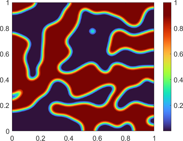 |
 |
 |
The first step of (78) is performed using BDF1 for the initial condition with a varying ratio of the areas occupied by each state, as shown in Figure 6. The initial snapshots are computed themselves with FOM simulations of the discretized equation (77) on with and from the initial random Bernoulli distribution with probability of equal to , respectively, at each of nodes of the spatial discretization grid. Thus, we consider a three-parameter system, i.e., , with the parameter domain .
Once the -snapshots are calculated via (78), -snapshots are simply
| (79) |
We use a grid of log-uniformly distributed values in , three values of and three values of to define the sampling set .
| 0.1 | 0.01 | ||||
|---|---|---|---|---|---|
| TT-ranks | |||||
| TT-ranks | |||||
| 1902 | 555 | 226 | |||
| 6921 | 870 | 274 | 123 | 69 |
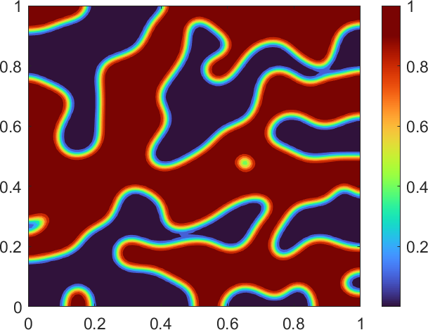
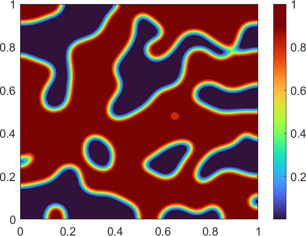
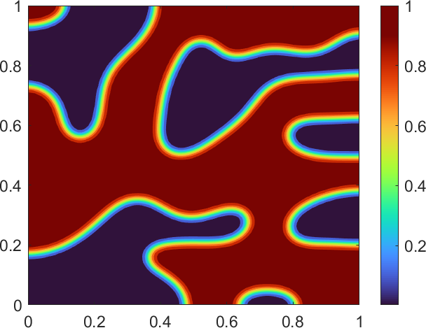
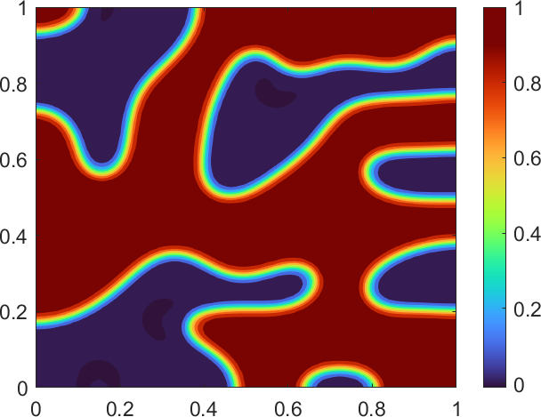
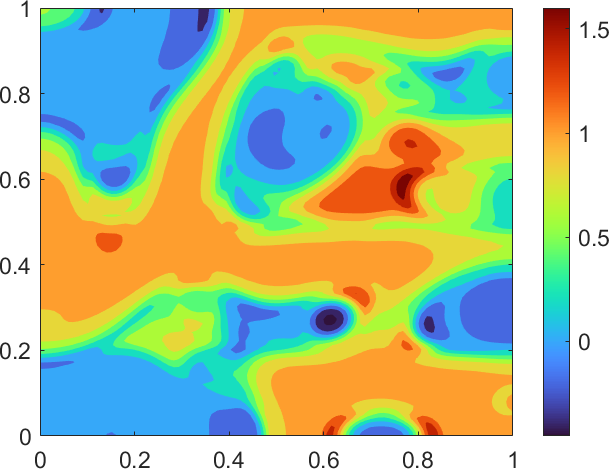
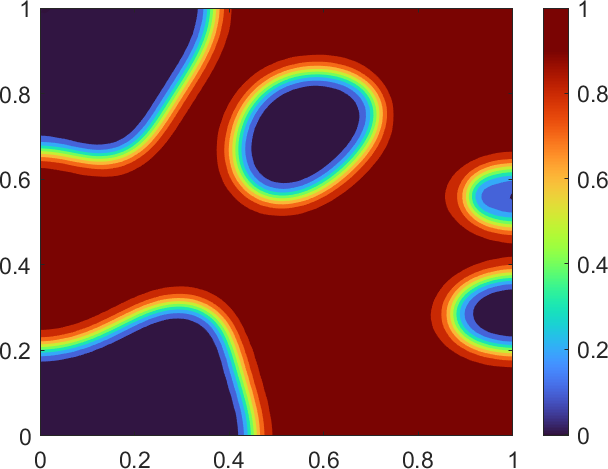
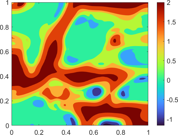
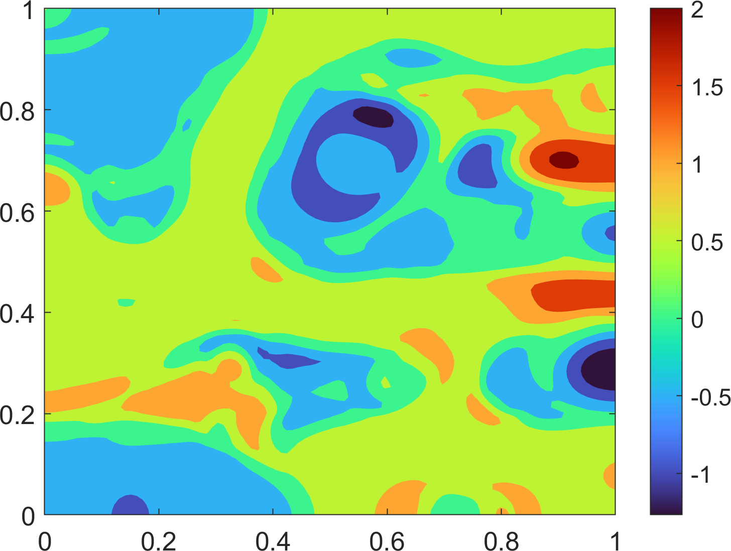
In the first experiment we study in-sample representation capacity of TT-TROM and compare it to that of POD–DEIM ROM. In Figure 7 we display the FOM, TT-TROM and POD–DEIM ROM solutions of discretized Allen–Cahn equation at the terminal time for two in-sample parameter vectors. The TT-TROM solution was computed for tensor compression accuracy . Decreasing compression accuracy to did not lead to a visual difference in TT-TROM solutions. The corresponding tensor ranks and compression factors for different values of are summarized in Table 3. We observe that while TT-TROM with the modest local reduced space dimensions predicts the pattern evolution very well, the conventional POD–DEIM ROM is inaccurate.
| FOM | TT-TROM | POD-DEIM ROM |
|---|---|---|
 |
 |
 |
 |
 |
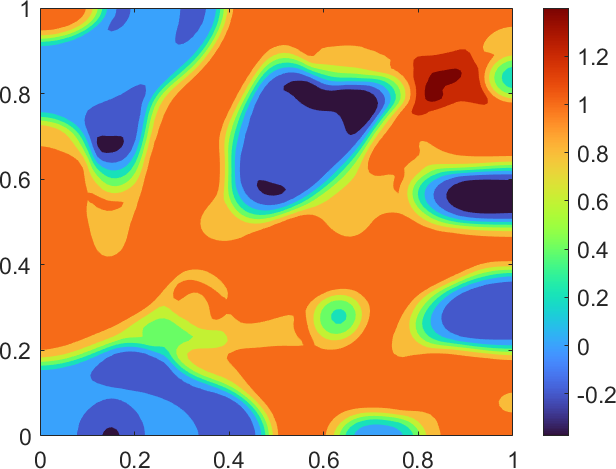 |
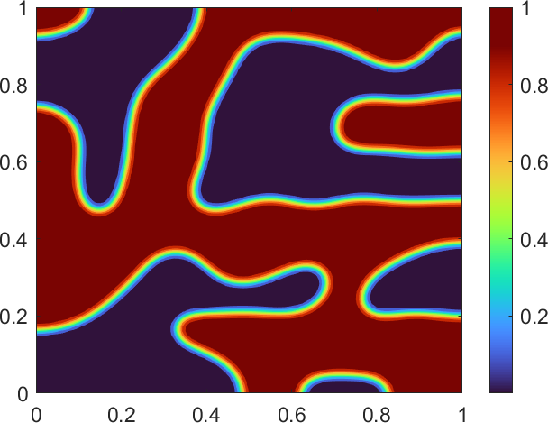
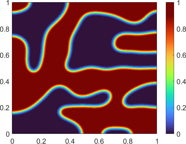
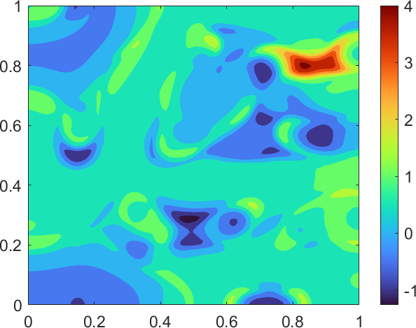
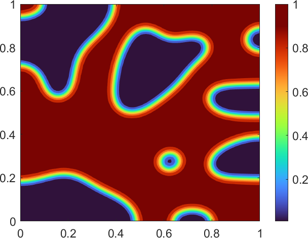
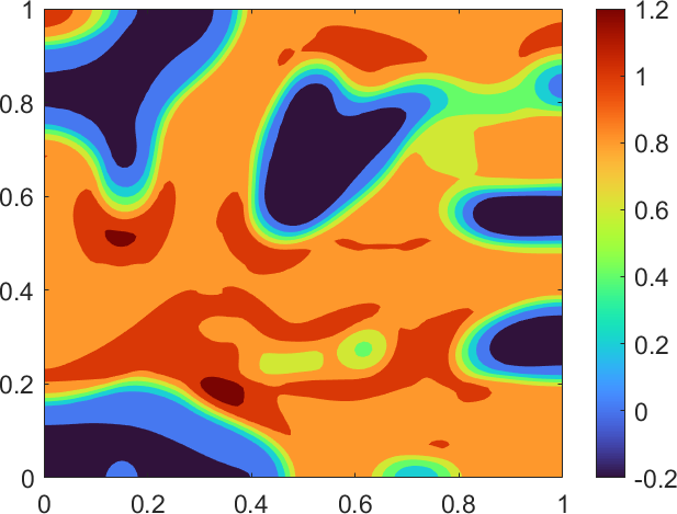
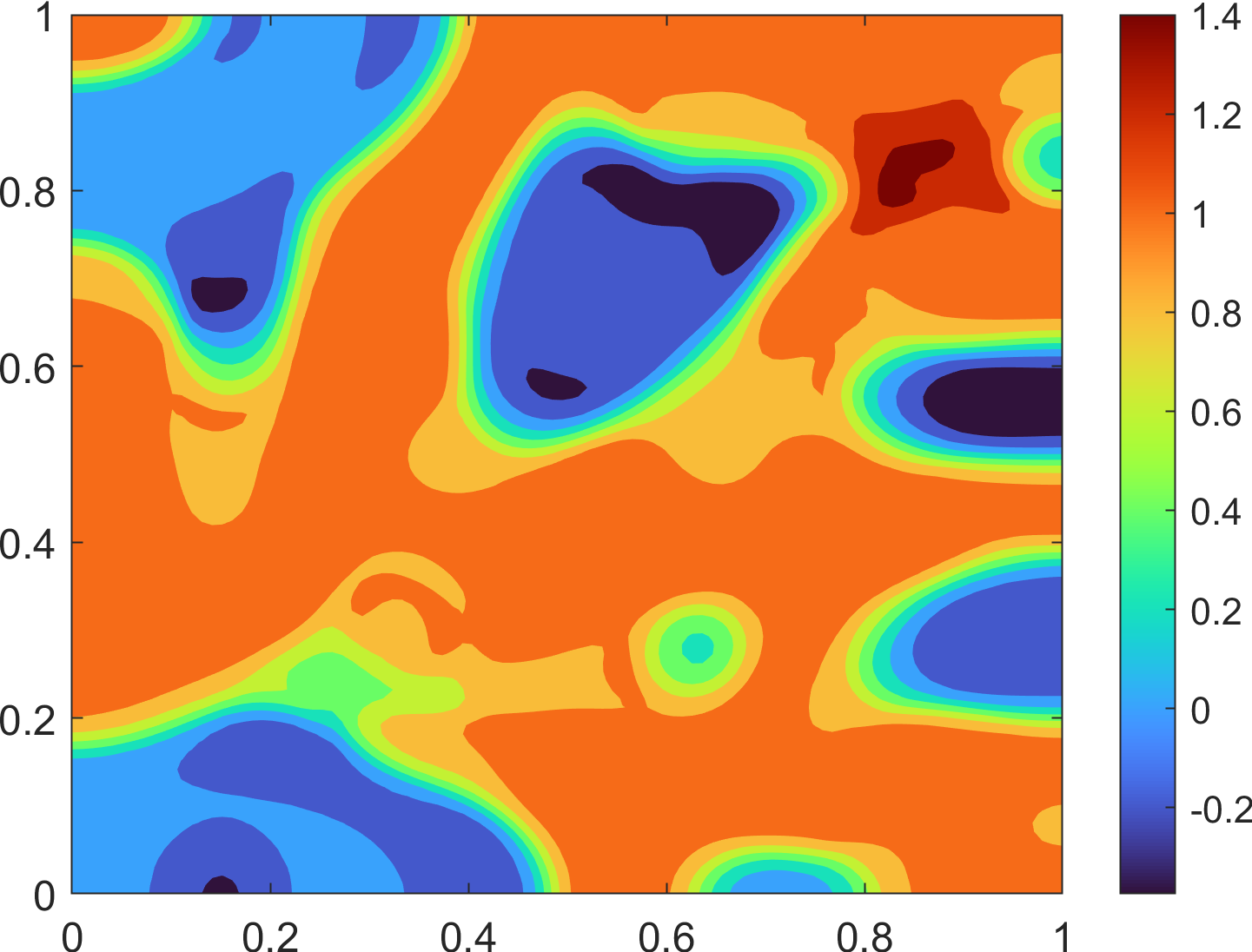
Next, we repeat the experiment for out-of-sample parameter values. We disply in Figure 8 the FOM, TT-TROM and POD–DEIM ROM solutions of discretized Allen–Cahn equation at the terminal time for two out-of-sample parameter vectors. We observe again an excellent prediction offered by TT-TROM, although the relative error increased from about for the in-sample case to about for the out-of-sample case. Similarly, POD–DEIM ROM once again fails to accurately predict the solutions.
| FOM | TT-TROM | POD-DEIM ROM |
|---|---|---|
 |
 |
 |
 |
 |
 |
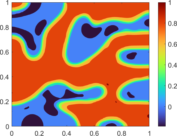 |
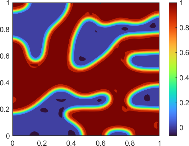 |
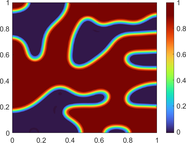 |
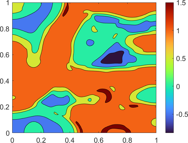
Finally, we examine the effect of varying tensor compression accuracy on TROM solution accuracy and compression ranks. In Figure 9 we display the TT-TROM solutions of discretized Allen–Cahn equation at for an out-of-sample parameter vector for the three different values of with local reduced space dimensions equal to the effective ranks, i.e., for both . In Table 3 we observe a large ratio of the first to last TT-ranks which is even higher than that for the example in Section 7.1. This explains a vast accuracy gain offered by the TT-TROM compared to the conventional POD–DEIM ROM. Indeed, POD–DEIM ROM performs poorly for this example with solutions being inaccurate even for larger local spaces dimensions, as demonstrated in Figure 10.
 |
 |
 |
 |
 |
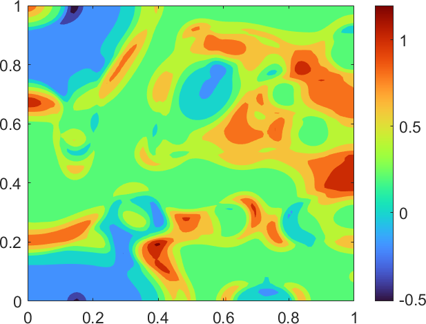 |
The computational times for the TT-TROM online stage in this Allen-Cahn equation example were mainly determined by the tensor compression ranks, as indicated in Table 3. For tensor compression accuracies , the average elapsed computational times on a laptop, calculated over multiple runs of the TT-TROM, were approximately 0.012 sec., 0.021 sec., and 0.040 sec., respectively. These times encompass steps 1 to 3 of the online stage in Algorithm 1, as well as the time required for integrating the projected system. This can be compared to an average time of 6 sec. required by the FOM for a single value of .
8 Conclusions
We introduced a Galerkin-type model order reduction framework for non-linear parametric dynamical systems that utilizes LRTD in place of POD for both projection and hyper-reduction steps. The LRTD is applied to find “universal” reduced spaces representing all observed snapshots and it is also used for finding “local” parameter-specific reduced subspaces of these larger universal spaces. If HOSVD or TT algorithms are employed to compute LRTD of snapshot tensors, then the universal spaces coincide with the POD spaces for the matrices of all observed snapshots. In this case, the proposed TROM can be also thought of as a tensor modification of the conventional POD–DEIM model reduction approach that benefits from the intrinsic tensor structure of a parametric system in several ways: (i) it provides means to find local spaces; (ii) it allows interpolation in the parameter domain directly in the reduced order spaces and thus enables efficient handling of parameters outside of the training set; (iii) it admits a rigorous analysis of the representation power of the reduced spaces for general parameter values.
We assessed the performance of three LRTD variants for model order reduction, based on CP, HOSVD and TT tensor formats. While TT was found to have a slight edge over HOSVD in terms of compression rates for the examples considered, the CP variant is in general more time consuming to compute and delivers worse approximation quality. Another variation considered is the approach to hyper-reduction in a two-stage setting. Out of the two variants we prefer the one with DEIM at the offline stage and local least squares at the online stage, since it performs similarly to the approach with DEIM on both stages, but also admits interpolation estimate for the local basis with a bound that is independent of parameters.
We note that for large scale FOMs and higher-dimensional parameter spaces, sampling full snapshot tensors may become prohibitively expensive due to the exponential increase of the number of snapshots as a function of the paratemeter space dimension. A promising approach to decrease the associated offline costs is the use of low-rank tensor interpolation or completion for finding LRTD from a sparse sampling of parameter domain. This should decouple the required number of parameter samples from the dimension of parameter space, assuming a certain degree of regularity in the dependence of dynamical system solutions on the parameters. Preliminary results suggesting feasibility and efficiency of such an approach will be reported in a forthcoming paper.
Acknowledgments
M.O. was supported in part by the U.S. National Science Foundation under awards DMS-2011444 and DMS-1953535. A.M. and M.O. were supported by the U.S. National Science Foundation under award DMS-2309197. This material is based upon research supported in part by the U.S. Office of Naval Research under award number N00014-21-1-2370 to A.M.
References
- [1] D. Amsallem and C. Farhat, Interpolation method for adapting reduced-order models and application to aeroelasticity, AIAA journal, 46 (2008), pp. 1803–1813.
- [2] D. Amsallem, M. J. Zahr, and C. Farhat, Nonlinear model order reduction based on local reduced-order bases, International Journal for Numerical Methods in Engineering, 92 (2012), pp. 891–916.
- [3] A. C. Antoulas, D. C. Sorensen, and S. Gugercin, A survey of model reduction methods for large-scale systems, tech. report, 2000.
- [4] U. Baur, C. Beattie, P. Benner, and S. Gugercin, Interpolatory projection methods for parameterized model reduction, SIAM Journal on Scientific Computing, 33 (2011), pp. 2489–2518.
- [5] P. Benner, S. Dolgov, A. Onwunta, and M. Stoll, Low-rank solvers for unsteady Stokes–Brinkman optimal control problem with random data, Computer Methods in Applied Mechanics and Engineering, 304 (2016), pp. 26–54.
- [6] P. Benner, S. Dolgov, A. Onwunta, and M. Stoll, Solving optimal control problems governed by random Navier–Stokes equations using low-rank methods, arXiv preprint arXiv:1703.06097, (2017).
- [7] P. Benner and L. Feng, A robust algorithm for parametric model order reduction based on implicit moment matching, in Reduced order methods for modeling and computational reduction, Springer, 2014, pp. 159–185.
- [8] P. Benner, S. Gugercin, and K. Willcox, A survey of projection-based model reduction methods for parametric dynamical systems, SIAM review, 57 (2015), pp. 483–531.
- [9] P. Benner, A. Onwunta, and M. Stoll, Low-rank solution of unsteady diffusion equations with stochastic coefficients, SIAM/ASA Journal on Uncertainty Quantification, 3 (2015), pp. 622–649.
- [10] S. L. Brunton, J. L. Proctor, and J. N. Kutz, Discovering governing equations from data by sparse identification of nonlinear dynamical systems, Proceedings of the national academy of sciences, 113 (2016), pp. 3932–3937.
- [11] T. Bui-Thanh, K. Willcox, and O. Ghattas, Model reduction for large-scale systems with high-dimensional parametric input space, SIAM Journal on Scientific Computing, 30 (2008), pp. 3270–3288.
- [12] J. D. Carroll and J.-J. Chang, Analysis of individual differences in multidimensional scaling via an n-way generalization of “Eckart-Young” decomposition, Psychometrika, 35 (1970), pp. 283–319.
- [13] S. Chaturantabut and D. C. Sorensen, Nonlinear model reduction via discrete empirical interpolation, SIAM Journal on Scientific Computing, 32 (2010), pp. 2737–2764.
- [14] L. De Lathauwer, B. De Moor, and J. Vandewalle, A multilinear singular value decomposition, SIAM journal on Matrix Analysis and Applications, 21 (2000), pp. 1253–1278.
- [15] P. Díez, S. Zlotnik, A. García-González, and A. Huerta, Algebraic pgd for tensor separation and compression: an algorithmic approach, Comptes Rendus Mécanique, 346 (2018), pp. 501–514.
- [16] J. L. Eftang, D. J. Knezevic, and A. T. Patera, An hp certified reduced basis method for parametrized parabolic partial differential equations, Mathematical and Computer Modelling of Dynamical Systems, 17 (2011), pp. 395–422.
- [17] J. L. Eftang, A. T. Patera, and E. M. Rønquist, An” hp” certified reduced basis method for parametrized elliptic partial differential equations, SIAM Journal on Scientific Computing, 32 (2010), pp. 3170–3200.
- [18] S. Gugercin and A. C. Antoulas, A survey of model reduction by balanced truncation and some new results, International Journal of Control, 77 (2004), pp. 748–766.
- [19] W. Hackbusch, Tensor spaces and numerical tensor calculus, vol. 42, Springer, 2012.
- [20] P. Hartman, Ordinary Differential Equations, vol. 590, John Wiley and Sons, 1964.
- [21] J. S. Hesthaven, G. Rozza, and B. Stamm, Certified reduced basis methods for parametrized partial differential equations, vol. 590, Springer, 2016.
- [22] F. L. Hitchcock, The expression of a tensor or a polyadic as a sum of products, Journal of Mathematics and Physics, 6 (1927), pp. 164–189.
- [23] S. Kastian, D. Moser, L. Grasedyck, and S. Reese, A two-stage surrogate model for neo-hookean problems based on adaptive proper orthogonal decomposition and hierarchical tensor approximation, Computer Methods in Applied Mechanics and Engineering, 372 (2020), p. 113368.
- [24] G. Kerschen, J.-c. Golinval, A. F. Vakakis, and L. A. Bergman, The method of proper orthogonal decomposition for dynamical characterization and order reduction of mechanical systems: an overview, Nonlinear dynamics, 41 (2005), pp. 147–169.
- [25] H. A. Kiers, Towards a standardized notation and terminology in multiway analysis, Journal of Chemometrics: A Journal of the Chemometrics Society, 14 (2000), pp. 105–122.
- [26] T. G. Kolda and B. W. Bader, Tensor decompositions and applications, SIAM review, 51 (2009), pp. 455–500.
- [27] D. Kressner and C. Tobler, Low-rank tensor Krylov subspace methods for parametrized linear systems, SIAM Journal on Matrix Analysis and Applications, 32 (2011), pp. 1288–1316.
- [28] K. Lee, H. C. Elman, and B. Sousedik, A low-rank solver for the Navier–Stokes equations with uncertain viscosity, SIAM/ASA Journal on Uncertainty Quantification, 7 (2019), pp. 1275–1300.
- [29] Y. Liang, H. Lee, S. Lim, W. Lin, K. Lee, and C. Wu, Proper orthogonal decomposition and its applications—part i: Theory, Journal of Sound and vibration, 252 (2002), pp. 527–544.
- [30] Y. Liang, W. Lin, H. Lee, S. Lim, K. Lee, and H. Sun, Proper orthogonal decomposition and its applications–part ii: Model reduction for mems dynamical analysis, Journal of Sound and Vibration, 256 (2002), pp. 515–532.
- [31] J. L. Lumley, The structure of inhomogeneous turbulent flows, Atmospheric turbulence and radio wave propagation, (1967).
- [32] A. V. Mamonov and M. A. Olshanskii, Interpolatory tensorial reduced order models for parametric dynamical systems, Computer Methods in Applied Mechanics and Engineering, 397 (2022), p. 115122.
- [33] A. Nouy, Low-rank tensor methods for model order reduction, arXiv preprint arXiv:1511.01555, (2015).
- [34] A. Nouy, Low-rank methods for high-dimensional approximation and model order reduction, Model reduction and approximation, P. Benner, A. Cohen, M. Ohlberger, and K. Willcox, eds., SIAM, Philadelphia, PA, (2017), pp. 171–226.
- [35] I. Oseledets and E. Tyrtyshnikov, TT-cross approximation for multidimensional arrays, Linear Algebra and its Applications, 432 (2010), pp. 70–88.
- [36] I. V. Oseledets, Tensor-train decomposition, SIAM Journal on Scientific Computing, 33 (2011), pp. 2295–2317.
- [37] M. Rathinam and L. R. Petzold, A new look at proper orthogonal decomposition, SIAM Journal on Numerical Analysis, 41 (2003), pp. 1893–1925.
- [38] J. Shen and X. Yang, Numerical approximations of Allen–Cahn and Cahn–Hilliard equations, Discrete & Continuous Dynamical Systems, 28 (2010), p. 1669.
- [39] L. Sirovich, Turbulence and the dynamics of coherent structures. i. coherent structures, Quarterly of applied mathematics, 45 (1987), pp. 561–571.
- [40] N. T. Son, A real time procedure for affinely dependent parametric model order reduction using interpolation on Grassmann manifolds, International Journal for Numerical Methods in Engineering, 93 (2013), pp. 818–833.
- [41] L. R. Tucker, Some mathematical notes on three-mode factor analysis, Psychometrika, 31 (1966), pp. 279–311.