FOSI: Hybrid First and Second Order Optimization

Abstract

Though second-order optimization methods are highly effective, popular approaches in machine learning such as SGD and Adam use only first-order information due to the difficulty of computing curvature in high dimensions. We present FOSI, a novel meta-algorithm that improves the performance of any first-order optimizer by efficiently incorporating second-order information during the optimization process. In each iteration, FOSI implicitly splits the function into two quadratic functions defined on orthogonal subspaces, then uses a second-order method to minimize the first, and the base optimizer to minimize the other. We prove FOSI converges and further show it improves the condition number for a large family of optimizers. Our empirical evaluation demonstrates that FOSI improves the convergence rate and optimization time of GD, Heavy-Ball, and Adam when applied to several deep neural networks training tasks such as audio classification, transfer learning, and object classification, as well as when applied to convex functions. Furthermore, our results show that FOSI outperforms other second-order methods such as K-FAC and L-BFGS.

1 Introduction

Consider the optimization problem $\min_{\theta}f(\theta)$ for a twice differential function $f:\mathbb{R}^{n}\rightarrow\mathbb{R}$. First-order optimizers such as gradient descent (GD) use only the gradient information to update $\theta$ (Kingma & Ba, 2014; Tieleman et al., 2012; Duchi et al., 2011; Polyak, 1987; Nesterov, 2003). Conversely, second-order optimizers such as Newton’s method update $\theta$ using both the gradient and the Hessian information. First-order optimizers are thus more computationally efficient as they only require evaluating and storing the gradient, and since their update step often involves only element-wise operations, but have a lower convergence rate compared to second-order optimizers in many settings (Tan & Lim, 2019). Unfortunately, second-order optimizers cannot be used for large-scale optimization problems such as deep neural networks (DNNs) due to the intractability of evaluating the Hessian when the dimension $n$ is large.

Despite recent work on hybrid optimizers that leverage second-order information without computing the entire Hessian (Henriques et al., 2019; Martens & Grosse, 2015; Gupta et al., 2018; Goldfarb et al., 2020), first-order methods remain the preferred choice for several reasons. First, many hybrid methods suffer from sensitivity to noisy Hessian approximations and have high computational requirements, making them less suitable for large-scale problems. Second, no single optimizer is best across all problems: the performance of an optimizer can depend on the specific characteristics of the problem it is being applied to (Nocedal & Wright, 1999; Wilson et al., 2017; Zhou et al., 2020).

Our Contributions.  We propose FOSI (for First-Order and Second-order Integration), an alternative approach, which instead of creating a completely new optimizer, improves the convergence of any base first-order optimizer by incorporating second-order information. FOSI works by iteratively splitting $\min_{\theta}f(\theta)$ into pairs of quadratic problems on orthogonal subspaces, then using Newton’s method to optimize one and the base optimizer to optimize the other. Unlike prior approaches, FOSI: (a) does not approximate the Hessian directly, and moreover only estimates the most extreme eignenvalues and vectors, making it more robust to noise; (b) has low and controllable overhead, making it usable for large-scale problems like DNNs; (c) accepts a base first-order optimizer, making it well suited for a large variety of tasks; and (d) works as “turn key” replacement for the base optimizer without additional tuning. We make the following contributions:

• A detailed description of the FOSI algorithm and a thorough spectral analysis of its preconditioner. We prove FOSI converges under common assumptions, and that it improves the condition number of the problem for a large family of base optimizers.

• An empirical evaluation of FOSI on common DNN training tasks with standard datasets, showing it improves over popular first-order optimizers in terms of convergence and wall time. The best FOSI optimizer achieves the same loss as the best first-order algorithm in 48%–77% of the wall time, depending on the task. We also use quadratic functions to explore different features of FOSI, showing it significantly improves convergence of base optimizers when optimizing ill-conditioned functions with non-diagonally dominant Hessians.

• A prototype open source implementation of FOSI, available at: https://github.com/hsivan/fosi .

2 Background and Notation

Given $\theta_{t}$, the parameter vector at iteration $t$, second-order methods incorporate both the gradient $g_{t}=\nabla f(\theta_{t})$ and the Hessian $H_{t}=\nabla^{2}f(\theta_{t})$ in the update step, while first-order methods use only the gradient. These algorithms typically employ an update step of the form $\theta_{t+1}=\theta_{t}+d_{t}$, where $d_{t}$ is a descent direction determined by the information (first and/or second order) from current and previous iterations. Usually, $d_{t}$ is of the form $-P_{t}^{-1}\bar{g}_{t}$, where $P_{t}$ is a preconditioner matrix and $\bar{g}_{t}$ is a linear combination of current and past gradients. This results in an effective condition number of the problem given by the condition number of $P_{t}^{-1}H_{t}$, which ideally is smaller than that of $H_{t}$ (Zupanski, 2002). Note that in Newton’s method $P_{t}=H_{t}$, resulting is an ideal effective condition number of 1; however, evaluating the Hessian for large $n$ is intractable and thus, most first-order methods are limited to preconditioners that approximate the Hessian diagonal (Sun & Spall, 2021; Zupanski, 2002).

The Lanczos algorithm.  We can obtain information about the curvature of a function $f$ without computing its entire Hessian. The Lanczos algroithm (Lanczos, 1950) is an iterative method that finds the $m$ extreme eigenvalues and eigenvectors of a symmetric matrix $A\in\mathbb{R}^{n\times n}$, where $m$ is usually much smaller than $n$. After running $m$ iterations, its output is a matrix $U\in\mathbb{R}^{n\times m}$ with orthonormal columns and a tridiagonal real symmetric matrix $T\in\mathbb{R}^{m\times m}$. To extract the approximate eigenvalues and eigenvectors of $A$, let $Q\Lambda Q^{T}$ be the eigendecomposition of $T$, s.t. $\Lambda$ is a diagonal matrix whose diagonal is the eigenvalues of $T$ sorted from largest to smallest and $Q$’s columns are their corresponding eigenvectors. The approximate $k$ largest and $\ell$ smallest eigenvalues of $A$ are the first $k$ and last $\ell$ elements of $\Lambda$’s diagonal, and their approximate corresponding eigenvectors are the first $k$ and last $\ell$ columns of the matrix product $UQ$.

The Lanczos approximation is more accurate for more extreme eigenvalues, thus to accurately approximate the $k$ largest and $\ell$ smallest eigenvalues, $m$ must be larger than $k+\ell$. Crucially, the Lanczos algorithm does not require storing $A$ explicitly. It only requires an operator that receives a vector $v$ and computes the matrix-vector product $Av$. In our case, $A$ is the Hessian $H_{t}$ of $f(\theta)$ at the point $\theta_{t}$. We denote by $hvp_{t}(v):\mathbb{R}^{n}\rightarrow\mathbb{R}$ the operator that returns the Hessian vector product $H_{t}v$. This operator can be evaluated in linear time (roughly two approximations of $f$’s gradient), using Pearlmutter’s algorithm (Pearlmutter, 1994).

Notations and definitions.  We use $\operatorname{diag}(v)$ for a diagonal matrix with diagonal $v$, $\mathbf{0}_{m}$ or $\mathbf{1}_{m}$ for a row vector of zeros or ones of size $m$, and $[A,B]$ for concatenating two matrices $n\times m_{1}$, $n\times m_{2}$ into a single $n\times(m_{1}+m_{2})$ matrix. The following notations are w.r.t a real symmetric matrix $A$ with eigenvalues $\lambda_{1}>\mathinner{\ldotp\kern-1.99997pt\ldotp\kern-1.99997pt\ldotp}>\lambda_{n}$ and eigenvectors $v_{1},\mathinner{\ldotp\kern-1.99997pt\ldotp\kern-1.99997pt\ldotp},v_{n}$:

$\widehat{\lambda}$    a row vector whose entries are $\lambda_{1},\mathinner{\ldotp\kern-1.99997pt\ldotp\kern-1.99997pt\ldotp},\lambda_{k}$ and
$\widecheck{V}$ $\lambda_{n-\ell+1},\mathinner{\ldotp\kern-1.99997pt\ldotp\kern-1.99997pt\ldotp},\lambda_{n}$ (the $k$ largest and $\ell$ smallest).
$\widehat{V}$    $\mathbb{R}^{n\times k+\ell}$ matrix whose columns are the corresponding
$\widecheck{V}$ eigenvectors of the eigenvalues in $\widehat{\lambda}$.
$\widecheck{\lambda}$    a row vector whose entries are $\lambda_{k+1},\mathinner{\ldotp\kern-1.99997pt\ldotp\kern-1.99997pt\ldotp},\lambda_{n-\ell}$.
$\widecheck{V}$ $\mathbb{R}^{n\times n-k-\ell}$ matrix whose columns are corresponding
$\widecheck{V}$ eigenvectors of the eigenvalues in $\widecheck{\lambda}$.
$u$    a row vector equals to $1/\lvert\widehat{\lambda}\rvert$.

3 First and Second-Order Integration

FOSI is a hybrid method that combines a first-order base optimizer with Newton’s method by utilizing each to operate on a distinct subspace of the problem. The Lanczos algorithm, which provides curvature information of a function, is at the core of FOSI. We first discuss the heuristic for determining the parameter $m$ (number of Lanczos iterations) and provide an algorithm for approximating extreme eigenvalues and eigenvectors (§3.1). We then present FOSI (§3.2) and analyze its preconditioner (§3.3 and §3.4). We then discuss use of momentum (§3.5), a stochastic modification for DNN training (§3.6), support for closed-form learning rates (§3.8), spectrum estimation error (§3.9), and FOSI’s overhead (§3.10).

3.1 Extreme Spectrum Estimation (ESE)

FOSI uses the Lanczos algorithm to estimate the extreme eigenvalues and vectors of the Hessian $H_{t}$. Recently, Urschel (2021) presented probabilistic upper and lower bounds on the relative error of this approximation for arbitrary eigenvalues. While the upper bound is dependent on the true eigenvalues of $H_{t}$, which is unknown, the lower bound is dependent solely on $m$ and $n$. To maintain the lower bound small, it is necessary to set $m$ such that $m=\Theta(\ln n)$ and $m$ must be greater than $k+\ell$. We thus define a heuristic for determining $m$: $m=\max\{4(k+\ell),2\ln n\}.$

We now describe the ESE procedure for obtaining the $k$ largest and $\ell$ smallest eigenvalues of $H_{t}$ and their corresponding eigenvectors using Lanczos. ESE takes in the function $f$ and its parameter value $\theta_{t}$ as inputs and uses them to define the $hvp_{t}$ operator. The procedure then calls the Lanczos algorithm with a specified number of iterations, $m$, and the $hvp_{t}$ operator. We use a version of Lanczos that performs full orthogonalization w.r.t all previous vectors in each iteration to prevent numerical instability (Meurant & Strakoš, 2006). Finally, the algorithm extracts the desired eigenvalues and eigenvectors from Lanczos’s outputs. The steps are summarized in Appendix A as Algorithm 2.

3.2 The FOSI Optimizer

Algorithm 1 FOSI Optimizer.

0:  

1:  BaseOptStep: given gradient, return descent direction.

2:  $T$: number of iterations between two ESE runs.

3:  $W$: number of warmup iterations before calling ESE.

4:  $k,\ell$: parameters for ESE, $1\leq k+\ell\ll n$.

5:  $\alpha$: positive learning rate (scalar).

6:  $u\leftarrow\mathbf{0},\widehat{V}\leftarrow\mathbf{0}$.

6:   UpdateStep($\theta$, $g$, $\widehat{V}$, $u$)

7:  $g_{1}\leftarrow\widehat{V}\left(\widehat{V}^{T}g\right)$,  $g_{2}\leftarrow g-\widehat{V}\left(\widehat{V}^{T}g\right)$

8:  $d_{1}\leftarrow-\alpha\widehat{V}\left(\left(\widehat{V}^{T}g_{1}\right)\odot u^{T}\right)$

9:  $d_{b}\leftarrow$ BaseOptStep($g_{2}$)

10:  $d_{2}\leftarrow d_{b}-\widehat{V}\left(\widehat{V}^{T}d_{b}\right)$

11:  $\theta\leftarrow\theta+d_{1}+d_{2}$

12:  return $\theta$

12:   Optimize($f$, $\theta_{0}$)

13:  $t\leftarrow 0$

14:  while $\theta_{t}$ not converged do

15:     if $t>=W$ and $(t-W)\mod T=0$ then

16:        $\widehat{\lambda},\widehat{V}\leftarrow$ ESE($f,\theta_{t},k,\ell$)

17:        $u\leftarrow 1/\lvert\widehat{\lambda}\rvert$

18:     $g_{t}\leftarrow\nabla f(\theta_{t})$

19:     $\theta_{t+1}\leftarrow$ UpdateStep($\theta_{t}$, $g_{t}$, $\widehat{V}$, $u$)

20:     $t\leftarrow t+1$

Algorithm 1 provides the pseudocode for FOSI, which receives as input the base optimizer, the function to be optimized, and an initial point, and continues to perform optimization steps until convergence is reached. Parentheses in lines 7–10 are important as they allow for only matrix-vector products, reducing computational complexity. FOSI calls the ESE procedure every $T$ iterations to obtain $u$, the inverse of $k$ largest and $\ell$ smallest eigenvalues of $H_{t}$, and $\widehat{V}$, the corresponding eigenvectors. For simplicity, we defer the discussion of Lanczos approximation errors to §3.9. The first call to the ESE procedure is postponed by a specified number of warmup iterations denoted by $W$. During these iterations, the updates are equivalent to those of the base optimizer, as $u$ and $\widehat{V}$ are initialized as zeros. Recent studies have shown that popular techniques for weight initialization often result in a plateau-like initial point (Orvieto et al., 2022) where the Lanczos algorithm performs poorly. The warmup iterations are used to improve this condition.

FOSI computes the gradient at each iteration and updates $\theta_{t}$ using the UpdateStep procedure, which includes five steps:

1. Compute $g_{1}$, which is the sum of $g$’s projections on $\widehat{V}$’s columns, and $g_{2}$, which is the sum of $g$’s projections on $\widecheck{V}$’s columns. Due to the orthogonality of the eigenvectors, $g_{1}$ and $g_{2}$ are also orthogonal to each other.

2. Compute the descent direction $d_{1}=-\alpha\widehat{V}((\widehat{V}^{T}g_{1})\odot u^{T})$, where $\odot$ stands for the Hadamard product. While the chance of encountering an eigenvalue that is exactly or nearly 0 when using small $k$ and $\ell$ values is very small, it is common to add a small epsilon to $\lvert\widehat{\lambda}\rvert$ to avoid division by such values (Kingma & Ba, 2014) when computing $u$ (line 17). Note that an equivalent computation to $d_{1}$ is $-\alpha\widehat{V}\operatorname{diag}(u)\widehat{V}^{T}g$, which is an $\alpha$-scaled Newton’s method step that is limited to $\widehat{V}$ subspace. The resulting $d_{1}$ is a linear combination of $\widehat{V}$’s columns.

3. Call the base optimizer to compute a descent direction from $g_{2}$, denoted by $d_{b}$.

4. Subtract from $d_{b}$ its projection on $\widehat{V}$’s columns and assign the result to $d_{2}$. The new vector $d_{2}$ is orthogonal to $\widehat{V}$’s columns, hence also to $d_{1}$.

5. Update the parameters: $\theta_{t+1}=\theta_{t}+d_{1}+d_{2}$

At each iteration $t$ of the optimization process, FOSI implicitly uses the quadratic approximation of $f$, $\tilde{f}=f_{t}+(\theta-\theta_{t})^{T}g_{t}+\frac{1}{2}(\theta-\theta_{t})^{T}H_{t}(\theta-\theta_{t})$, and performs a step to minimize this quadratic function. To minimize $\tilde{f}$, FOSI first divides the vector space that is the eigenvectors of $H_{t}$ into two orthogonal complement subspaces – one is spanned by $\widehat{V}$’s columns and the other by $\widecheck{V}$. It then implicitly splits $\tilde{f}$ into two functions $f_{1}$ and $f_{2}$ such that $\tilde{f}$ is their sum:
$f_{1}=\frac{1}{2}f_{t}+(\theta-\theta_{t})^{T}g_{1}+\frac{1}{2}(\theta-\theta_{t})^{T}\widehat{V}\operatorname{diag}(\widehat{\lambda})\widehat{V}^{T}(\theta-\theta_{t})\text{,}$ $f_{2}=\frac{1}{2}f_{t}+(\theta-\theta_{t})^{T}g_{2}+\frac{1}{2}(\theta-\theta_{t})^{T}\widecheck{V}\operatorname{diag}(\widecheck{\lambda}){\widecheck{V}}^{T}(\theta-\theta_{t})\text{.}$ We observe that $\tilde{f}=f_{1}+f_{2}$, since $g_{t}=g_{1}+g_{2}$ and $H_{t}=\widehat{V}\operatorname{diag}(\widehat{\lambda})\widehat{V}^{T}+\widecheck{V}\operatorname{diag}(\widecheck{\lambda}){\widecheck{V}}^{T}$. Moreover, $f_{1}$ is a quadratic function with similar slope and curvature as $\tilde{f}$ in the subspace that is spanned by $\widehat{V}$ and zero slope and curvature in its orthogonal complement $\widecheck{V}$. Similarly, $f_{2}$ is a quadratic function with similar slope and curvature as $\tilde{f}$ in the subspace that is spanned by $\widecheck{V}$ and zero slope and curvature in its orthogonal complement $\widehat{V}$.

Finally, FOSI minimizes $f_{1}$ and $f_{2}$ independently: it uses a scaled Newton’s step to minimize $f_{1}$, and the base optimizer step to minimize $f_{2}$. To minimize $f_{1}$, FOSI changes $\theta$ in the direction $d_{1}$ that is a linear combination of $\widehat{V}$’s columns, and to minimize $f_{2}$, it changes $\theta$ in the direction $d_{2}$ that is a linear combination of $\widecheck{V}$’s columns. Hence, we can look at each step of FOSI as two simultaneous and orthogonal optimization steps that do not affect the solution quality of each other, and their sum is a step in the minimization of $\tilde{f}$.

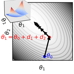
(a) $f$

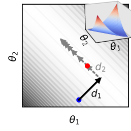
(b) $f_{1}$

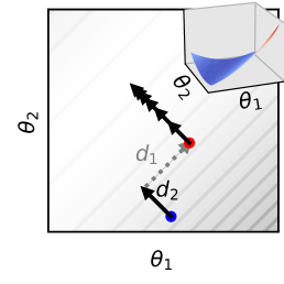
(c) $f_{2}$

Figure 1: FOSI’s update steps (arrows) when minimizing a quadratic function $f(\theta)$ with GD as the base optimizer. FOSI implicitly separates the vector space $V$, which is the set of eigenvectors of $f$’s Hessian, into two orthogonal complement subspaces and then splits the original function into two function $f_{1}$ and $f_{2}$ over these subspaces, s.t. $f=f_{1}+f_{2}$. FOSI solves $\min f$ by simultaneously solving $\min f_{1}$ with Newton’s method and $\min f_{2}$ with GD. The update step is the sum of $d_{1}$ and $d_{2}$, the updates to $f_{1}$ and $f_{2}$ respectively.

Figure 1 illustrates this concept. The function $f(\theta)=1.25\theta_{1}^{2}+1.25\theta_{2}^{2}+1.5\theta_{1}\theta_{2}$ has two eigenvalues, $\lambda_{1}=4$, $\lambda_{2}=1$, with the eigenvectors $v_{1}=[1/\sqrt{2},1/\sqrt{2}]^{T}$, $v_{2}=[-1/\sqrt{2},1/\sqrt{2}]^{T}$. The subspaces are $\widehat{V}=\{v_{1}\}$, $\widecheck{V}=\{v_{2}\}$. Since $f$ is quadratic, its Hessian is constant, so a quadratic approximation of $f$ around any point is exactly $f$, and the split to $f_{1}$ and $f_{2}$ is unique: $f_{1}=\theta_{1}^{2}+\theta_{2}^{2}+2\theta_{1}\theta_{2}$ and $f_{2}=0.25\theta_{1}^{2}+0.25\theta_{2}^{2}-0.5\theta_{1}\theta_{2}$. To solve $\min f_{1}$ FOSI uses Newton’s method. The update $d_{1}$ is parallel to $v_{1}$ and since $f_{1}$ is quadratic, this update brings $f_{1}$ to its minimum in one step. To solve $\min f_{2}$ FOSI uses the base optimizer, in this case GD, and the update $d_{2}$ is parallel to $v_{2}$. Since $f_{1}$ is constant along $v_{2}$ direction, an update to $\theta$ in this direction does not impact its value, and similarly for $f_{2}$ with $v_{1}$ direction. The sum $d_{1}+d_{2}$ is the update applied to $\theta$. The next updates are only affected by updates to $f_{2}$, since $f_{1}(\theta_{1})$ is at its minimum so $d_{1}$ is always zero.

We next analyze FOSI as a preconditioner. For simplicity, the $t$ subscript is omitted from $g_{t}$ and $H_{t}$ when it is clear from the text that the reference is to a specific point in time.

3.3 Diagonal Preconditioner

For base optimizers that utilize a diagonal matrix as a preconditioner (e.g., Adam), the result is an efficient computation, as $P^{-1}g$ is equivalent to element-wise multiplication of $P^{-1}$’s diagonal with $g$. When using FOSI with such a base optimizer, the diagonal of the inverse preconditioner, denoted by $q$, is calculated using $g_{2}$, instead of $g$. Hence, $d_{b}=-\eta\operatorname{diag}(q)g_{2}$, for some learning rate $\eta>0$.

Lemma 3.1.

Let $f(\theta)$ be a convex twice differential function and let BaseOpt be a first-order optimizer that utilizes a positive definite (PD) diagonal preconditioner. Let $H$ be $f$’s Hessian at iteration $t$ of Algorithm 1 with BaseOpt, and let $V\operatorname{diag}(\lambda)V^{T}$ be an eigendecomposition of $H$ such that $V=[\widehat{V},\widecheck{V}]$ and $\lambda=[\widehat{\lambda},\widecheck{\lambda}]$. Then:

1. FOSI’s inverse preconditioner is

   $$P^{-1} =V\left(\begin{array}[]{cc}\alpha\operatorname{diag}(u)&\mathbf{0}\\ \mathbf{0}&\eta M\\ \end{array}\right)V^{T},$$

   where $M$ is the trailing $n-k-\ell$ principal submatrix (lower right corner submatrix) of $V^{T}\operatorname{diag}(q)V$, and $\operatorname{diag}(q)$ is the inverse preconditioner produced by BaseOpt from $g_{2}$.

2. The preconditioner $P$ is symmetric and PD.

3. $\alpha$ is an eigenvalue of the effective Hessian $P^{-1}H$, and $\widehat{V}$’s columns are in the eigenspace of $\alpha$.

The proof can be found in Appendix B. It includes expressing $d_{1}$ and $d_{2}$ as a product of certain matrices with $g$, substituting these expressions into $\theta_{t}+d_{1}+d_{2}$, and using linear algebra properties to prove that the resulting preconditioner is a symmetric PD matrix. Finally, we assign $P^{-1}$ expression to obtain $P^{-1}H$. Note that symmetric PD preconditioner is necessary for ensuring that the search direction always points towards a descent direction (Li, 2017).

As expected, we obtained a separation of the space into two subspaces. For the subspace that is spanned by $\widehat{V}$, for which FOSI uses scaled Newton’s method, the condition number is 1. For the complementary subspace, the condition number is determined by BaseOpt’s preconditioner. In the general case, it is hard to determine the impact of a diagonal preconditioner on the condition number of the problem, although it is known to be effective for diagonally dominant Hessian (Qu et al., 2020; Levy & Duchi, 2019). Appendix D includes an analysis of the special case in which $H$ is diagonal. We show that even in this case, which is ideal for a diagonal preconditioner, FOSI provides benefit, since it solves $f_{1}$ with Newton’s method and provides the base optimizer with $f_{2}$, which is defined on a smaller subspace, hence can be viewed as of smaller dimensionality than $f$.

3.4 Identity Preconditioner

The identity preconditioner is a special case of the diagonal preconditioner where all diagonal entries are the same. For base optimizers with identity preconditioner such as GD, we obtain a complete spectral analysis of FOSI’s preconditioner and effective Hessian, even for non-diagonal Hessian.

Lemma 3.2.

Under the same assumption as in Lemma 3.1, with BaseOpt that utilizes a scaled identity inverse preconditioner $\eta I$ for some learning rate $\eta>0$:

1. FOSI’s resulting inverse preconditioner is
   $P^{-1}=V\operatorname{diag}([\alpha u,\eta\mathbf{1}_{n-k-\ell}])V^{T}.$

2. The preconditioner $P$ is symmetric and PD.

3. $\alpha$ is an eigenvalue of the effective Hessian $P^{-1}H$, and $\widehat{V}$’s columns are in the eigenspace of $\alpha$. In addition, the entries of the vector $\eta\widecheck{\lambda}$ are eigenvalues of $P^{-1}H$ and their corresponding eigenvectors are $\widecheck{V}$’s columns.

The proof, following from Lemma 3.1 by replacing $\operatorname{diag}(q)$ with $\eta I$, can be found in Appendix C.

As in the diagonal case, the condition number of the subspace that is spanned by $\widehat{V}$ is 1. The condition number of $\widecheck{V}$ is $\lambda_{k+1}/\lambda_{n-\ell}$. Both condition numbers, of $f_{1}$ and $f_{2}$, are smaller than the condition number of $H$. Since we have a complete spectral analysis of $P^{-1}H$ we can obtain the effective condition number and the conditions in which it is smaller than the original one. However, since FOSI uses two optimizers on orthogonal subspaces, a more relevant measure for improvement is whether the effective condition number of each subspace is smaller then the original one. Appendix E provides the analysis of the effective condition number. It also shows an example in which FOSI’s condition number is larger than the original one, but FOSI improves the convergence since it improves the condition number of each subspace separately.

3.5 Momentum

Momentum accelerates convergence of first-order optimizers and is adapted by many popular optimizers (Qian, 1999; Kingma & Ba, 2014). When using momentum, the descent direction is computed on $\bar{g}$, instead of $g$, where $\bar{g}$ is a linear combination of the current and past gradients. $\bar{g}$ is defined differently by different optimizers. Momentum could also be used by FOSI; however, FOSI and the base optimizer must apply the same linear combination on $g_{1}$ and $g_{2}$ to maintain FOSI’s correctness, i.e., maintain the orthogonality of $f_{1}$ and $f_{2}$. Applying the same linear combination entails $\bar{g}=\bar{g_{1}}+\bar{g_{2}}$. We can use $\bar{g},\bar{g_{1}},\bar{g_{2}}$ in the proof of Lemma 3.1, instead of $g,g_{1},g_{2}$ and obtain similar results.

3.6 Stochastic Setting

We adopt the stochastic setting proposed by Wang et al. (2017). Consider the stochastic optimization problem $\min_{\theta}f(\theta)$ for $f(\theta)=\mathbb{E}_{x}[F(\theta,x)]$, where $F:\mathbb{R}^{n}\times\mathbb{R}^{d}\rightarrow\mathbb{R}$ is twice differentiable w.r.t $\theta$ and $x\in\mathbb{R}^{d}$ denotes a random variable with distribution $P$. When stochastic optimization is used for DNN training, $f$ is usually approximated by a series of of functions: at each iteration $t$ of the optimization, a batch $b_{t}$ containing $m_{t}$ data samples $\{x_{1},x_{2},\mathinner{\ldotp\kern-1.99997pt\ldotp\kern-1.99997pt\ldotp},x_{m_{t}}\}$ is sampled and the function $f^{t}$ is set as $f^{t}(\theta)=\frac{1}{m_{t}}\sum_{i=1}^{m_{t}}F(\theta,x_{i})$. Note that labels, if any, can be added to the data vectors to conform to this model.

Adapting FOSI to stochastic DNN training requires a small change to Algorithm 1. at the beginning of each iteration of the algorithm, the first action would be to sample a batch $b_{t}$ and set $f^{t}$. We can call the ESE procedure with the current $f^{t}$, or with some predefined $f^{i},i\leq t$, as discussed in §3.9.

3.7 Convergence Analysis

We now show convergence of FOSI in the common stochastic setting under common Lipschitz smoothness assumptions on $f$ and $F$, and assuming bounded noise level of the stochastic gradient.

Lemma 3.3.

Let BaseOpt be a first-order optimizer that utilizes a PD diagonal preconditioner and denote by $\nabla^{2}F(\theta,x)=\frac{\partial^{2}F}{\partial\theta^{2}}$ the Hessian of $F$ w.r.t $\theta$. Assuming:

1. $f(\theta)$ is $L$-smooth and lower bounded by a real number.

2. For every iteration $t$, $\mathbb{E}_{x_{t}}[\nabla_{\theta}F(\theta_{t},x_{t})]=\nabla f(\theta_{t})$ and $\mathbb{E}_{x_{t}}[\left\lVert\nabla_{\theta}F(\theta_{t},x_{t})-\nabla f(\theta_{t})\right\rVert^{2}]\leq\sigma^{2}$, where $\sigma>0$, $x_{t}$ for $t=1,2,\mathinner{\ldotp\kern-1.99997pt\ldotp\kern-1.99997pt\ldotp}$ are independent samples, and for a given $t$ the random variable $x_{t}$ is independent of $\{\theta_{i}\}_{i=1}^{t}$.

3. There exist a positive constant $z$ s.t. for every $\theta$ and $x$, $\left\lVert\nabla^{2}F(\theta,x)\right\rVert\leq z$ and the diagonal entries of BaseOpt’s preconditioner are upper bounded by $z$.

Then, for a given $\epsilon\in(0,1)$, the number of iterations $N$ needed to obtain $\frac{1}{N}\sum_{t=1}^{N}\mathbb{E}\left[\left\lVert\nabla f(\theta_{t})\right\rVert^{2}\right]\leq\epsilon$ when applying FOSI with BaseOpt is $N=O\left(\epsilon^{-\frac{1}{1-\beta}}\right)$, for step size $\eta$ chosen proportional to $t^{-\beta}$, where $\beta\in(0.5,1)$ is a constant.

The proof (in Appendix F) works by expressing FOSI in the form of the stochastic quasi-Newton method used in Theorem 2.8 of (Wang et al., 2017), and proving the Theorem’s conditions are satisfied.

3.8 Automatic Learning Rate Scaling

When the base optimizer has a closed-form expression of its optimal learning rate in the quadratic setting that is only dependant on the extreme eigenvalues, FOSI can adjust a tuned learning rate $\eta$ to better suit the condition number of $f_{2}$. Fortunately, in most cases of optimizers that utilize a diagonal preconditioner, such as GD, Heavy-Ball, and Nesterov, there are such closed-forms (Lessard et al., 2016).

Specifically, when applying FOSI with such a base optimizer and given the relevant closed-form expression for the optimal learning rate, the adjusted learning rate at iteration $t$ would be $\eta_{2}=\eta(\eta_{2}^{*}/\eta^{*})$, where $\eta^{*}$ is the optimal learning rate for the quadratic approximation $\tilde{f}$ and $\eta_{2}^{*}$ is the optimal one for $f_{2}$. FOSI is able to compute this scaling, as it obtains the relevant extreme eigenvalues from the ESE procedure.

The intuition behind this scaling is that the ratio between the optimal learning rates is proportional to the ratio between the condition number of $\tilde{f}$ and that of $f_{2}$. The full details regarding this scaling technique are in Appendix G.

Note that the scaling factor $\eta_{2}^{*}/\eta^{*}$ is greater than or equal to 1. In practice, we suggest a more conservative scaling that involves clipping over this scaling factor as follows: $\eta_{2}=\eta\min\{\eta^{*}_{2}/\eta^{*},c\}$ for $c\geq 1$. For $c=1$, $\eta_{2}=\eta$, and for extremely large $c$ ($\infty$), the scaling factor is not clipped.

3.9 ESE Approximation Error

Using Newton’s method in non-quadratic settings in conjunction with inexact approximation of Hessian eigenvalues through the ESE procedure increases the risk of divergence. To mitigate this, we employ a scaled Newton’s method, with a learning rate of $0<\alpha\leq 1$, for function $f_{1}$, as an alternative to the traditional Newton’s method which enforces $\alpha=1$. We also mitigate issues of numerical accuracy in the ESE procedure. Using float32 can lead to significant errors, while using float64 throughout the training demands excessive memory and computation time. To balance precision and performance, we use float64 only for the ESE procedure computations and retain the original precision for the function’s parameters and other computations. To mitigate problem in Lanczos convergence caused by a plateau-like initial point (Orvieto et al., 2022), we use warmup iterations before the first ESE call. Finally, the use of the ESE procedure in a stochastic setting could theoretically result in unsuitable $\widehat{V}$ and $\widehat{\lambda}$ when called with $f^{i}$ which misrepresent $f$. Techniques to address this include using larger batch size only for the ESE procedure, or averaging the results obtained from different $f^{i}$s. We leave the investigation of such techniques to future work. In practice, our experiments on a variety of DNNs in §4, using an arbitrary $f^{j}$ on ESE calls, demonstrate that FOSI is robust and substantially improves convergence.

3.10 Runtime and Memory Overhead

Runtime.  FOSI’s runtime differs from that of the base optimizer due to additional computations in each update step and calls to the ESE procedure. For large and complex functions, the latency of the update step of both optimizers, the base optimizer and FOSI, is negligible when compared to the computation of the gradient in each iteration. Furthermore, since each Lanczos iteration is dominated by the Hessian-vector product operation which takes approximately two gradient evaluations, the latency of the ESE procedure can be approximated by $2m\tau$, where $\tau$ is gradient computation latency and $m$ the number of Lanczos iterations (see §3.1). The ESE procedure is called every $T$ iterations, hence the parameter $T$ impacts FOSI’s runtime relative to the base optimizer. Since the improvement in convergence rate for any given $T$ is not known in advance, the parameter $T$ should be set such that FOSI’s runtime is at most $\rho$ times the base optimizer runtime, for a user-defined overhead $\rho>1$. Thus, given the above approximations and assumptions, we can achieve overhead $\rho$ by setting: $T=2m/(\rho-1).\quad~{}(1)$ This heuristic helps avoid the need to tune $T$, though FOSI can of course use any $T>0$. See Appendix H for additional details as well as a more accurate expression for $T$ for functions where additional computations are not negligible in comparison to gradient computations.

Memory.  FOSI stores $k+\ell$ eigenvectors of size $O(n)$, and temporarily uses $O(mn)$ memory when performing the ESE procedure by maintaining the Lanczos matrix U. In comparison, other second order methods such as K-FAC (Martens & Grosse, 2015) and Shampoo (Gupta et al., 2018) incur $O(\sum_{i\in L}d_{i}^{2}+p_{i}^{2})$ memory overhead, where $d_{i}$ is the input dimension of layer $i$, $p_{i}$ the output dimension, and $L$ is the total number of layers. While less than $O(n^{2})$, it is not linear and can substantially exceed $n$ when there are layers with $p_{i}\neq d_{i}$. For example, for $d_{i}=1000$ and $d_{i}=10$, FOSI with $m=40$ requires approximately 400K parameters while K-FAC requires approximately 1M parameters.

4 Evaluation

We first validate our theoretical results by evaluating FOSI on a positive definite (PD) quadratic function with different base optimizers; we explore the effect of the dimension $n$, the eigenspectrum, the learning rate, the base optimizer, and the clipping parameter $c$ on FOSI’s performance. We then evaluate FOSI’s performance on benchmarks tasks including real-world DNNs with standard datasets, for both first- and second-order methods.

Setup.  We implemented FOSI in Python using the JAX framework (Bradbury et al., 2018) 0.3.25. For experiments, we use an NVIDIA A40 GPU with 48 GB of RAM.

4.1 Quadratic Functions

To evaluate FOSI’s optimization performance across range of parameters, we use controlled experiments on PD quadratic functions of the form $f_{H}(\theta)=0.5\theta^{T}H\theta$. We use GD, Heavy-Ball (HB), and Adam optimizers to minimize $f_{H}$, as well as FOSI with these base optimizers. We use the default momentum parameters $\beta_{1}=0.9,\beta_{2}=0.999$ for Adam and $\beta=0.9$ for HB. The learning rate $\eta$ for Adam was set to $0.05$ after tuning, for GD it was set to $2/(\lambda_{1}+\lambda_{2})$ which is the optimal value, and for HB we used $2/(\sqrt{\lambda_{1}}+\sqrt{\lambda_{n}})^{2}$ which is half of the optimal value (due to using constant $\beta$ rather than optimal). FOSI runs with $k=10$, $\ell=0$, $\alpha=1$, and $c=\infty$ (no clipping on the scaling of the GD and HB learning rates, see §3.8).

Dimensionality and ill-conditioning.  To study the effect of dimensionality and eigenspectrum on FOSI, we created five $f_{H}$ functions for each $n\in\{100,1500\}$ by varying $\lambda_{1}$ of the Hessian $H$ with $\lambda_{1}\in\{5,10,20,50,200\}$. The other eigenvalues were set to $\lambda_{i}=1.5^{-(i-2)}$ and the eigenvectors were extracted from a symmetric matrix whose entries were randomly sampled from $U(0,1)$.

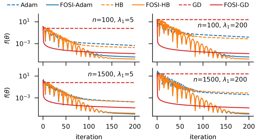
Figure 2: Learning curves of optimizers for minimizing PD quadratic functions $f_{H}(\theta)=0.5\theta^{T}H\theta$ with varying dimensionality $n$ and $\lambda_{1}$ value. FOSI converges much faster, more than two orders of magnitude, than its counterparts.

Figure 2 shows learning curves of the optimizers on functions with $\lambda_{1}=5$ and $\lambda_{1}=200$. Similar results were obtained for other functions. FOSI converges at least two orders of magnitude faster than its counterparts. In this case, dimensionality has little impact on the performance of different optimizers. For a specific $n$ value, increasing $\lambda_{1}$ causes the base optimizers to converge to less optimal solutions, but has little impact on FOSI. This is expected for GD and HB, whose learning rate is limited by the inverse of the largest eigenvalue, hence, larger $\lambda_{1}$ implies slower convergence. FOSI reduces the largest eigenvalue, allowing for larger learning rate that is identical for all functions. Interestingly, this is observed for Adam as well.

Ill-conditioning and diagonally dominance.  We explore the effect of both the condition number and the diagonally dominance of the function’s Hessian on the different optimizers. To do so, we define a set of functions $f_{b,\zeta}(\theta)=0.5\theta^{T}H_{b,\zeta}\theta$ for $b\in\{1.1,\mathinner{\ldotp\kern-1.99997pt\ldotp\kern-1.99997pt\ldotp},1.17\}$ and $\zeta\in\{0,\mathinner{\ldotp\kern-1.99997pt\ldotp\kern-1.99997pt\ldotp},100\}$, $\theta\in\mathbb{R}^{100}$, where $b$ and $\zeta$ are parameters that define the Hessian $H_{b,\zeta}$. The parameter $b$ determines the eigenvalues of $H_{b,\zeta}$: $\forall i\in\{1,\mathinner{\ldotp\kern-1.99997pt\ldotp\kern-1.99997pt\ldotp},100\}$ $\lambda_{i}=0.001b^{i}$. The parameter $\zeta$ determines the number of rows in $H_{b,\zeta}$ that are not dominated by the diagonal element, i.e., the part of $H_{b,\zeta}$ which is not diagonally dominant. We set the initial point s.t. $f_{b,\zeta}(\theta_{0})$ is identical for all functions with the same $b$ value. The full details regarding the constructions of $H_{b,\zeta}$ and the method of setting $\theta_{0}$ are in Appendix I.

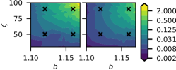
(a) Adam (right) vs. FOSI-Adam (left)

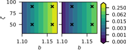
(b) HB (right) vs. FOSI-HB (left)

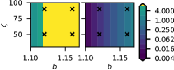
(c) GD (right) vs. FOSI-GD (left)

Figure 3: Each $(b,\zeta)$ combination in each sub figure is the value of different $f_{b,\zeta}$ after 200 iterations of the optimizer. FOSI improves over the base optimizer for every function. Learning curves for four functions, indicated by black x markers, can be found in Appendix I.

Figure 3 shows $f_{b,\zeta}$ at the optimal point after 200 iterations of the optimizers for different $b$ and $\zeta$ values. For a specific $b$ value, rotations of the coordinate system (changes in $\zeta$) have no impact on GD and HB, as seen by the vertical lines with the same value for different $\zeta$ values. Their performance deteriorates for larger $b$ values (more ill-conditioned problems). When applying FOSI, the new maximal eigenvalues of two functions with similar $\zeta$ and different $b$ are still differ by an order of magnitude, which leads to the differences in FOSI’s performance along the $b$ axis. Adam’s performance is negatively affected for large $b$ and $\zeta$ values. FOSI improves over the base optimizer in all cases. Due to space limitations, a detailed analysis of the learning curves can be found in Appendix I.

Learning rate and momentum.  we explored the effect of various learning rates and momentum parameters on the optimizers. We find that FOSI improves over Adam, HB, and GD for all learning rates and momentum (for HB and Adam). The full details of this experiment are in Appendix J.

4.2 Deep Neural Networks

We evaluated FOSI on five DNNs of various sizes using standard datasets, first focusing first-order methods in common use. We execute FOSI with $k=10$ and $\ell=0$, since small eigenvalues are usually negative. We set $\alpha=0.01$, $c=3$, and $W$ such that warmup is one epoch. $T$ is determined using equation (3.10) aiming at 10% overhead ($\rho=1.1$), resulting in $T=800$ for all experiments. The base optimizers compared to FOSI are HB (momentum) and Adam; we omit GD (SGD) as it performed worse than HB in most cases. We use the standard learning rate for Adam ($0.001$), and the best learning rate for HB out of ${0.1,0.01,0.001}$, with default momentum parameters $\beta_{1}=0.9,\beta_{2}=0.999$ for Adam and $\beta=0.9$ for HB.

The five evaluated tasks are:

1. Audio Classification (AC): Training MobileNetV1 (approximately 4 million parameters) on the AudioSet dataset (Gemmeke et al., 2017). The dataset contains about 20,000 audio files, each 10 seconds long, with 527 classes and multiple labels per file. We converted the audio files into 1-second mel-spectrograms and used them as input images for the DNN. The multi-hot label vector of a segment is the same as the original audio file’s label.

2. Language Model (LM): Training an RNN-based character-level language model with over 1 million parameters on the Tiny Shakespeare dataset (Karpathy, 2015). For LM training batches are randomly sampled; hence, there is no defined epoch and we use $W=T$.

3. Autoencoder (AE): Training an autoencoder model with roughly 0.5 million parameters on the CIFAR-10 dataset. We observed that the HB optimizer in this case is sensitive to the learning rate and diverges easily. Therefore we run FOSI with $c=1$ (prevents learning rate scaling) and $W=T$, which enables extra warmup iterations (number of iteration per epoch is 175).

4. Transfer Learning (TL): Transfer learning from ImageNet to CIFAR-10. We start with a pre-trained ResNet-18 on ImageNet2012 and replace the last two layers with a fully-connected layer followed by a Softmax layer. We train the added fully-connected layer (5130 params), while the other layers are frozen (11 million parameters).

5. Logistic Regression (LR): Training a multi-class logistic regression model to predict the 10 classes of the MNIST dataset. The model is a neural network with one fully connected layer of 784 input size followed by a Softmax layer of 10 outputs, containing 7850 parameters. The input data is the flattened MNIST images. Since logistic regression is a convex function, the model is also convex w.r.t. the parameters of the network.

Table 1: Wall time to reach target validation accuracy (AC, TL, LR) or loss (LM, AE), in seconds. The target accuracy/loss (in parentheses) is the best one reached by the base optimizer. No single base optimizer is best for all tasks.

Task	HB	FOSI-HB		Adam	FOSI-Adam
AC	3822	1850	(40.4%)	5042	3911	(28.9%)
LM	269	207	(1.71)	270	219	(1.76)
AE	354	267	(52.46)	375	313	(51.26)
TL	93	53	(79.1%)	68	33	(79.0%)
LR	16	8	(92.8%)	12	18	(92.8%)

Table 1 summarize the experimental results, showing the wall time when reaching a target validation accuracy (for AC, TL, LR tasks) or target validation loss (for LM, AE tasks). The target metric (in parentheses) is the best one reached by the base optimizer.

FOSI consistently reaches the target metric faster than the base optimizer (though Adam is faster than FOSI-Adam on LR, FOSI-HB is faster than both). The improvement in FOSI-HB is more significant than in FOSI-Adam, due to FOSI-HB’s ability to adapt the learning rate according to the improved condition number of the effective Hessian.

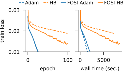
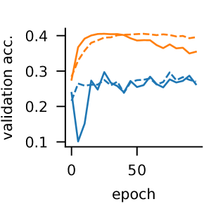
Figure 4: Training AC (MobileNetV1 on AudioSet data). FOSI converges faster than HB across epochs (left) and wall time (middle), and similar to Adam. Adam overfits and generalizes poorly as indicated by its validation accuracy (right).

Figure 4 shows the optimizers’ learning curves for the AC task. The training loss curves suggests that FOSI significantly improves the performance of HB, but does not help Adam. However, while Adam’s training loss reaches zero quickly, it suffers from substantial overfitting and generalizes poorly, as indicated by its accuracy. This supports the idea that there is no single best optimizer for all problems (Zhou et al., 2020). FOSI aims to improve the best optimizer for each specific task. In this case, HB is preferred over Adam as it generalizes much better, and FOSI improves over HB. It is important to note that when the base optimizer overfits, FOSI’s acceleration of convergence also leads to an earlier overfitting point. This can be observed in the validation accuracy curve: HB begins to overfit near epoch 70 while FOSI begins to overfit at roughly epoch 35.

Summary.  FOSI improves convergence of the base optimizer, and is the fastest optimizer for all five tasks. On average, FOSI achieves the same loss as its base optimizer in 78% of the time on the training set and the same accuracy/loss in 75% of the time on the validation set. Additional details for each experiment can be found in table 2 in Appendix K, along with additional learning curves for all tasks.

4.3 Comparison to Second-Order Methods

We compare FOSI to two widely used second-order techniques, K-FAC (Martens & Grosse, 2015) and L-BFGS (Liu & Nocedal, 1989) by repeating the five DNN training experiments and comparing the results of both algorithms to FOSI-HB. We use the KFAC-JAX (Botev & Martens, 2022) implementation for K-FAC and the JAXOpt library (Blondel et al., 2021) for L-BFGS.

We used grid search to tune K-FAC’s learning rate and momentum, and included K-FAC’s adaptive as one of the options. We utilized adaptive damping and maintained the default and more precise $T_{3}$ (interval between two computations of the approximate Fisher inverse matrix) value of 5 after testing larger $T_{3}$ values and observing no variation in runtime. For tuning L-BFGS hyperparameters, we used line-search for the learning rate, and performed a search for the optimal $L$ (history size) for each task, starting from $L=10$ (similar to $k$ we used for FOSI) and up to $L=100$. The hyperparameters were selected based on the lowest validation loss obtained for each experiment.

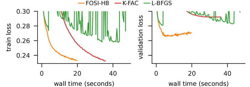
Figure 5: Learning curves of FOSI-HB, K-FAC, and L-BFGS for the LR training task. FOSI converges faster to a lower validation loss than K-FAC and L-BFGS.

Overall, we observed that both K-FAC and L-BFGS algorithms have slower runtimes and poorer performance compared to FOSI. They occasionally diverge, can overfit, and rarely achieve the same level of validation accuracy as FOSI. Specifically:

• LR: K-FAC converges quickly but overfits dramatically, resulting in much higher validation loss than FOSI. L-BFGS converges much more slowly than the other approaches and to a much higher validation loss. Figure 5 shows the learning curves of the optimizers.

• TL: Both K-FAC and L-BFGS converge slower than FOSI and result in higher validation loss.

• AE: K-FAC converges quickly but is noisy and leads to a large validation loss (52.1 compared to 51.4 for FOSI), while L-BFGS diverges quickly after the first epoch, even with large values of $L$.

• LM: we could not get the K-FAC implementation to work on this RNN model (this is a known issue with K-FAC and RNN (Martens et al., 2018)). L-BFGS converges more slowly, and to a much higher loss.

• AC: K-FAC converges slower than FOSI and shows substantial overfitting, while L-BFGS does not converge.

See Appendix K for additional results for each experiment.

5 Related Work

Second-order optimizers employ the entire Hessian in the optimization process (Nocedal & Wright, 1999). Newton’s method calculates the inverse Hessian in each iteration, while BFGS method uses an iterative approach to approximate the inverse Hessian. These methods are not suitable for large-scale functions such as DNNs due to their high computational and storage requirements.

Partially second-order optimizers are a group of optimization methods that incorporate some aspects of second-order information in their optimization process. L-BFGS (Liu & Nocedal, 1989) is a memory-efficient variant of BFGS method, useful for training large-scale functions. However, its performance is affected by the parameter controlling the number of previous iterations used to approximate the Hessian, and an incorrect selection can lead to slow convergence or divergence. Additionally, it requires line search in each iteration, slowing down the optimization process further.

Recent approaches in optimization of DNNs exploit the structure of the network to approximate a block diagonal preconditioner matrix, as an alternative to full second-order methods. K-FAC (Martens & Grosse, 2015) and Shampoo (Gupta et al., 2018) use a block diagonal approximation of the Fisher matrix, where each block corresponds to a different layer of the DNN, while K-BFGS (Goldfarb et al., 2020) approximates the Hessian. However, these methods are still computationally and storage intensive, making them less suitable for large-scale problems. While techniques have been proposed to reduce memory overhead, such as skipping preconditioning for some layers (Pauloski et al., 2021), these methods can be similarly applied to FOSI.

Other optimization approaches for stochastic settings involve the use of sub-sampling of $f^{i}$ functions and constructing an approximation of the Hessian based on the gradients of these functions at each iteration (Roosta-Khorasani & Mahoney, 2019; Xu et al., 2016). However, these methods are limited to functions with only a few thousand parameters. CurveBall (Henriques et al., 2019) interleaves conjugate-gradient steps and weight updates, resulting in Heavy-Ball’s update step with additional curvature information. Note that CurveBall is limited to improving Heavy-Ball.

Finally, while these works propose a single improved optimizer, FOSI is a meta-optimizer that improves the performance of a base first-order optimizer.

6 Discussion and Future Work

FOSI is a hybrid meta-optimizer that combines any first-order method with Newton’s method to improve the optimization process. Rather than rely on a single approach, FOSI accepts a base first-order optimizer and improves it without additional tuning – making it particularly suitable as a plug-in replacement for optimizers with existing tasks. Moreover, FOSI’s runtime overhead is modest and can be set directly. Evaluation on real and synthetic tasks demonstrates FOSI improves the wall time to convergence when compared to the base optimizer.

Future research will focus on methods for automatic tuning of different parameters of FOSI, such as dynamically adjusting parameters $k$ and $\ell$ according to their impact on the effective condition number. We also plan to investigate the effect of stale spectrum estimation, which could allow running the ESE procedure on the CPU in parallel to the training process on the GPU.

Appendix A The ESE Algorithm

Algorithm 2 details ESE procedure for obtaining the $k$ largest and $\ell$ smallest eigenvalues, as well as their corresponding eigenvectors, of the Hessian $H_{t}$ using Lanczos. The details of the algorithm are in § 3.1.

Algorithm 2 Extreme Spectrum Estimation.

0:   ESE($f$, $\theta_{t}$, $k$, $\ell$)

  $n\leftarrow$ length of $\theta_{t}$

  $m\leftarrow\max\{4(k+\ell),2\ln n\}$

  $hvp_{t}\leftarrow$ generate $hvp$ operator from $f$ and $\theta_{t}$.

  $U,T\leftarrow$ Lanczos($m,hvp_{t}$)

  $Q,\Lambda\leftarrow$ eigendecomposition($T$)

  $\widehat{\lambda}\leftarrow$ first $k$ and last $\ell$ of $\Lambda$’s diagonal

  $\widehat{V}\leftarrow$ first $k$ and last $\ell$ columns of $UQ$

  return $\widehat{\lambda},\widehat{V}$

Appendix B Proof of Lemma 3.1 (Diagonal Preconditioner)

Proof.

In case we apply FOSI on an optimizer that uses an inverse diagonal preconditioner s.t. $d_{b}=-\eta\operatorname{diag}(q)g_{2}$, then:

$$d_{1} =-\alpha\widehat{V}\left(\left(\widehat{V}^{T}g_{1}\right)\odot u\right)=-\alpha\widehat{V}\left(\left(\underbrace{\widehat{V}^{T}\widehat{V}}_{I}\left(\widehat{V}^{T}g\right)\right)\odot u\right)=-\alpha\widehat{V}\operatorname{diag}(u)\widehat{V}^{T}g,$$

$$d_{2} =d_{b}-\widehat{V}\left(\widehat{V}^{T}d_{b}\right)=\left(I-\widehat{V}\widehat{V}^{T}\right)d_{b}=-\eta\left(I-\widehat{V}\widehat{V}^{T}\right)\operatorname{diag}(q)g_{2}=-\eta\left(I-\widehat{V}\widehat{V}^{T}\right)\operatorname{diag}(q)\left(g-\widehat{V}\left(\widehat{V}^{T}g\right)\right)$$

$$=-\eta\left(I-\widehat{V}\widehat{V}^{T}\right)\operatorname{diag}(q)\left(I-\widehat{V}\widehat{V}^{T}\right)g.$$

By assigning these forms of $d_{1}$ and $d_{2}$ in the update step $\theta_{t+1}=\theta_{t}+d_{1}+d_{2}$, we obtain that the update step is of the form $\theta_{t+1}=\theta_{t}-P^{-1}g$ and the inverse preconditioner is:

$$P^{-1}=\alpha\widehat{V}\operatorname{diag}(u)\widehat{V}^{T}+\eta\left(I-\widehat{V}\widehat{V}^{T}\right)\operatorname{diag}(q)\left(I-\widehat{V}\widehat{V}^{T}\right).$$ (2)

Note that

$$\widehat{V}\operatorname{diag}(u)\widehat{V}^{T}=V\operatorname{diag}([u,\mathbf{0}_{n-k-\ell}])V^{T}.$$ (3)

Similarly, and using the fact that $V$ is an orthonormal matrix ($V$ is an orthogonal basis) and hence $VV^{T}=I$:

$$I-\widehat{V}\widehat{V}^{T} =VIV^{T}-V\operatorname{diag}([\mathbf{1}_{k+\ell},\mathbf{0}_{n-k-\ell}])V^{T}$$

$$=V\left(I-\operatorname{diag}([\mathbf{1}_{k+\ell},\mathbf{0}_{n-k-\ell}])\right)V^{T}$$

$$=V\operatorname{diag}([\mathbf{0}_{k+\ell},\mathbf{1}_{n-k-\ell}])V^{T}.$$ (4)

By assigning (3) and (B) in (2) we obtain:

$$P^{-1}= \alpha V\operatorname{diag}([u,\mathbf{0}_{n-k-\ell}])V^{T}+\eta V\operatorname{diag}([\mathbf{0}_{k+\ell},\mathbf{1}_{n-k-\ell}])V^{T}\operatorname{diag}(q)V\operatorname{diag}([\mathbf{0}_{k+\ell},\mathbf{1}_{n-k-\ell}])V^{T}$$

$$= V\bigr{[}\;\alpha\operatorname{diag}([u,\mathbf{0}_{n-k-\ell}])+\eta\operatorname{diag}([\mathbf{0}_{k+\ell},\mathbf{1}_{n-k-\ell}])V^{T}\operatorname{diag}(q)V\operatorname{diag}([\mathbf{0}_{k+\ell},\mathbf{1}_{n-k-\ell}])\;\bigr{]}V^{T}.$$

This completes the proof of claim 1 of the Lemma.

Note that multiplying a diagonal matrix from the left of another matrix is equivalent to scaling each row of the later by the corresponding diagonal entry of the former, and similarly multiplying a diagonal matrix from from the right has the same effect on columns. Therefore, the matrix

$$B= \operatorname{diag}([\mathbf{0}_{k+\ell},\mathbf{1}_{n-k-\ell}])V^{T}\operatorname{diag}(q)V\operatorname{diag}([\mathbf{0}_{k+\ell},\mathbf{1}_{n-k-\ell}])$$ (5)

is a matrix whose first $k+\ell$ rows and first $k+\ell$ columns are 0.

Denote by $M$ the sub matrix of $B$ that contains the entries $i,j$ s.t. $i,j>k+\ell$. Sine BaseOpt utilizes a PD preconditioner (as stated in the Lemma 3.1), i.e. $\operatorname{diag}(q)\succ 0$, hence $V^{T}\operatorname{diag}(q)V\succ 0$, and since $M$ is a trailing principal submatrix of $V^{T}\operatorname{diag}(q)V$ it is PD (Gentle, 2017, p. 349). $M$ is also symmetric, since $B$ is symmetric. The diagonal matrix $\operatorname{diag}(u)$ is also symmetric and PD. Since a block diagonal matrix is PD if each diagonal block is PD (Gallier et al., 2020) and symmetric if each block is symmetric, the block diagonal matrix

$$\alpha\operatorname{diag}([u,\mathbf{0}_{n-k-\ell}])+\eta B=\left(\begin{array}[]{cc}\alpha\operatorname{diag}(u)&\mathbf{0}\\ \mathbf{0}&\eta M\\ \end{array}\right)$$ (8)

is PD and symmetric.

Since $V$ has full column and row rank, and the block diagonal matrix (8) is PD, the inverse preconditioner

$$P^{-1} =V\left(\begin{array}[]{cc}\alpha\operatorname{diag}(u)&\mathbf{0}\\ \mathbf{0}&\eta M\\ \end{array}\right)V^{T}$$

is PD (Gentle, 2017, p. 113). It is also symmetric, as (8) is symmetric.

Finally, using the fact that the inverse of a PD and symmetric matrix is PD and symmetric, we conclude that the preconditioner $P$ is symmetric and PD. This completes the proof of claim 2 of the Lemma.

We assign the above $P^{-1}$ in $P^{-1}H$ to obtain the effective Hessian:

$$P^{-1}H= V\left(\begin{array}[]{cc}\alpha\operatorname{diag}(u)&\mathbf{0}\\ \mathbf{0}&\eta M\\ \end{array}\right)V^{T}V\operatorname{diag}([\widehat{\lambda},\widecheck{\lambda}])V^{T}$$

$$= V\left(\begin{array}[]{cc}\alpha\operatorname{diag}(u)\operatorname{diag}(\widehat{\lambda})&\mathbf{0}\\ \mathbf{0}&\eta M\operatorname{diag}(\widecheck{\lambda})\\ \end{array}\right)V^{T}$$

$$= V\left(\begin{array}[]{cc}\alpha\operatorname{diag}(\mathbf{1}_{k+\ell})&\mathbf{0}\\ \mathbf{0}&\eta M\operatorname{diag}(\widecheck{\lambda})\\ \end{array}\right)V^{T}.$$

We obtained a partial eigendecomposition of the effective Hessian, which indicates that there are at least $k+\ell$ repetitions of the eigenvalues with value $\alpha$ and its corresponding eigenvectors are $\widehat{V}$’s eigenvectors. This completes the proof of claim 3 of the Lemma. ∎

Appendix C Proof of Lemma 3.2 (Identity Preconditioner)

Proof.

The proof immediately follows from Lemma 3.1 by replacing $\operatorname{diag}(q)$ with $I$.

By replacing $\operatorname{diag}(q)$ with $I$ in (5), we obtain

$$B=\operatorname{diag}([\mathbf{0}_{k+\ell},\mathbf{1}_{n-k-\ell}])V^{T}IV\operatorname{diag}([\mathbf{0}_{k+\ell},\mathbf{1}_{n-k-\ell}])=\operatorname{diag}([\mathbf{0}_{k+\ell},\mathbf{1}_{n-k-\ell}]).$$

Hence, $M=\operatorname{diag}(\mathbf{1}_{n-k-\ell})$. Assigning this $M$ in $P^{-1}$ given by Lemma 3.1 obtains:

$$P^{-1} =V\left(\begin{array}[]{cc}\alpha\operatorname{diag}(u)&\mathbf{0}\\ \mathbf{0}&\eta\operatorname{diag}(\mathbf{1}_{n-k-\ell})\\ \end{array}\right)V^{T}=V\operatorname{diag}([\alpha u,\eta\operatorname{diag}(\mathbf{1}_{n-k-\ell})])V^{T},$$

which completes the proof of claim 1 of the Lemma.

$P^{-1}$ is diagonal matrix with positive diagonal entries, and therefore symmetric and PD. Its inverse, $P$, is also symmetric and PD, which completes the proof of claim 2 of the Lemma.

We assign the above $P^{-1}$ in $P^{-1}H$ to obtain the effective Hessian:

$$P^{-1}H=V\operatorname{diag}([\alpha u,\eta\mathbf{1}_{n-k-\ell}])V^{T}V\operatorname{diag}([\widehat{\lambda},\widecheck{\lambda}])V^{T}=V\operatorname{diag}([\alpha\mathbf{1}_{k+\ell},\eta\widecheck{\lambda}])V^{T}.$$

We obtained an eigendecomposition of the effective Hessian, which implies there are $k+\ell$ repetitions of the eigenvalues with value $\alpha$ and their corresponding eigenvectors are $\widehat{V}$’s columns, and the entries of $\eta\widecheck{\lambda}$ are eigenvalues and their corresponding eigenvectors are $\widecheck{V}$’s columns. This completes the proof of claim 3 of the Lemma. ∎

Appendix D Special Case Analysis: Diagonal Preconditioner Base Optimizer and Diagonal Hessian

In the special case in which the eigenvectors of $H$ are aligned to the axes of the Euclidean space $\mathbb{R}^{n}$ (i.e. $H$ is diagonal), $V$ is a permutation matrix (has exactly one entry of 1 in each row and each column and 0s elsewhere). Note that $I\operatorname{diag}(q)I^{T}$ is an eigendecomposition of $\operatorname{diag}(q)$. Let $\mathcal{P}$ be the permutation of $I$’s columns, such that $\mathcal{P}(I)=V$. Then $V\operatorname{diag}(\mathcal{P}(q))V^{T}$ is also an eigendecomposition of $\operatorname{diag}(q)$, i.e:

$$\operatorname{diag}(q)=V\operatorname{diag}(\mathcal{P}(q))V^{T}.$$

Therefore,

$$V^{T}\operatorname{diag}(q)V=V^{T}V\operatorname{diag}(\mathcal{P}(q))V^{T}V=\operatorname{diag}(\mathcal{P}(q)),$$

and $M$ is the $n-k-\ell$ trailing principal submatrix of $\operatorname{diag}(\mathcal{P}(q))$. In other words, the diagonal of $M$ contains the last $n-k-\ell$ entries of the vector $\mathcal{P}(q)$. By Lemma 3.1, $\alpha$ is an eigenvalue of $P^{-1}H$ with $k+\ell$ repetitions. From the analysis of $M$ we obtain that the remaining $n-k-\ell$ eigenvalues of $P^{-1}H$ are: $\eta\mathcal{P}(q)_{k+\ell+1}\lambda_{k+1},\mathinner{\ldotp\kern-1.99997pt\ldotp\kern-1.99997pt\ldotp},\eta\mathcal{P}(q)_{n}\lambda_{n-\ell}$. If $q$ is a good approximation to the Hessian diagonal, then these eigenvalues should be all close to $\eta$ since each $\mathcal{P}(q)_{i}$ is an approximation to the inverse of $\lambda_{i-\ell}$.

This is an optimal case, since the two optimization problems defined on the two subspaces have condition number of 1, which enable fast convergence. However, this is a very special case and the Hessian in most optimization problems is not diagonal. Moreover, even in this case, which is ideal for a diagonal preconditioner, FOSI provides benefit, since it solves $f_{1}$ with Newton’s method, which obtains an ideal effective condition number over $\widehat{V}$, and provides the base optimizer with $f_{2}$, which is defined on a smaller subspace $\widecheck{V}$, hence can be viewed as of smaller dimensionality than $f$.

Appendix E Analysis of the Effective Condition Number in the Identity Preconditioner Case

The following Lemma states the conditions in which the effective condition number is smaller than the original condition number when applying FOSI with a base optimizer that utilizes an identity preconditioner.

Lemma E.1.

Under the same assumption as in Lemma 3.2, denote the effective condition number induced by BaseOpt by $\kappa$ and the effective condition number induced by Algorithm 1 using BaseOpt by $\tilde{\kappa}$. Then, $\tilde{\kappa}\leq\kappa$ in the following cases:

1. $\alpha<\eta\lambda_{n-\ell}$ and $\frac{\eta\lambda_{k+1}}{\alpha}\leq\frac{\lambda_{1}}{\lambda_{n}}$

2. $\eta\lambda_{n-\ell}\leq\alpha\leq\eta\lambda_{k+1}$

3. $\eta\lambda_{k+1}<\alpha$ and $\frac{\alpha}{\eta\lambda_{n-\ell}}\leq\frac{\lambda_{1}}{\lambda_{n}}$

Proof.

The effective Hessian of an optimizer that utilizes a diagonal preconditioner $\eta I$ is $\eta H$. Therefore, $\kappa=(\eta\lambda_{1})/(\eta\lambda_{n})=\lambda_{1}/\lambda_{n}$, i.e. the preconditioner of such an optimizer does not change the condition number of the problem. As stated in claim 2 of Lemma 3.2, when using FOSI the distinct eigenvalues of the effective Hessian are $\alpha,\eta\lambda_{k+1},\mathinner{\ldotp\kern-1.99997pt\ldotp\kern-1.99997pt\ldotp},\eta\lambda_{n-\ell}$. There are now three distinct ranges for $\alpha$ which affect $\tilde{\kappa}$:

1. $\alpha<\eta\lambda_{n-\ell}$. In this case, the smallest eigenvalue of $P^{-1}H$ is $\alpha$ and the largest is $\eta\lambda_{k+1}$, which leads to $\tilde{\kappa}=\eta\lambda_{k+1}/\alpha$; therefore, $\tilde{\kappa}\leq\kappa\iff\frac{\eta\lambda_{k+1}}{\alpha}\leq\frac{\lambda_{1}}{\lambda_{n}}$.

2. $\eta\lambda_{n-\ell}\leq\alpha\leq\eta\lambda_{k+1}$. In this case, the smallest eigenvalue of $P^{-1}H$ is $\eta\lambda_{n-\ell}$ and the largest is $\eta\lambda_{k+1}$; therefore, $\tilde{\kappa}=\frac{\lambda_{k+1}}{\lambda_{n-\ell}}$ and $\tilde{\kappa}\leq\kappa\iff\frac{\lambda_{k+1}}{\lambda_{n-\ell}}\leq\frac{\lambda_{1}}{\lambda_{n}}$. Sine $\frac{\lambda_{k+1}}{\lambda_{n-\ell}}<\frac{\lambda_{1}}{\lambda_{n}}$ is true then $\tilde{\kappa}<\kappa$.

3. $\eta\lambda_{k+1}<\alpha$. In this case the smallest eigenvalue of $P^{-1}H$ is $\eta\lambda_{n-\ell}$ and the largest is $\alpha$; therefore, $\tilde{\kappa}=\frac{\alpha}{\eta\lambda_{n-\ell}}$ and $\tilde{\kappa}\leq\kappa\iff\frac{\alpha}{\eta\lambda_{n-\ell}}\leq\frac{\lambda_{1}}{\lambda_{n}}$.

∎

While Lemma E.1 provides the conditions in which FOSI improves the condition number, as discussed before, FOSI is able to accelerate the convergence of the optimization process even when it does not improve the condition number.

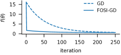
Figure 6: Learning curves of GD and FOSI for the minimization of the quadratic function $f(\theta)=0.5\theta^{T}H\theta$, with $\theta\in\mathbb{R}^{100}$. $H$’s eigenvectors are a random orthogonal basis, $\eta=0.001,\lambda_{1}=10,\lambda_{10}=9,\lambda_{n}=0.01$, and FOSI runs with $k=9,\ell=0,\alpha=1$. While FOSI’s effective condition number is larger than the original one, it converges much faster than the base optimizer.

To show this phenomenon, we use GD and FOSI with GD as a base optimizer to optimize the quadratic function $f(\theta)=0.5\theta^{T}H\theta,\theta\in\mathbb{R}^{100}$. We draw a random orthonormal basis for $f$’s Hessian, $H$, and set its eigenvalues as follows: $\lambda_{1},\mathinner{\ldotp\kern-1.99997pt\ldotp\kern-1.99997pt\ldotp},\lambda_{10}$ are equally spaced in the range $[9,10]$ and $\lambda_{11},\mathinner{\ldotp\kern-1.99997pt\ldotp\kern-1.99997pt\ldotp},\lambda_{100}$ are equally spaced in the range $[0.01,0.1]$. We used the learning rate $\eta=0.001$ and run FOSI with $k=9,\ell=0,\alpha=1$. For this setting we have $\lambda_{1}=10,\lambda_{10}=9,\lambda_{100}=0.01$ and none of the conditions in Lemma E.1 is satisfied. Since $\eta\lambda_{10}<1$, the only candidate condition in Lemma E.1 is condition (3), however, in this case FOSI’s effective condition number is $1/(\eta\lambda_{100})=100000$, which is much larger than the original condition number of the problem, which is $\lambda_{1}/\lambda_{100}=1000$. However, as shown in Figure 6, FOSI converges much faster then GD.

This example emphasises our claim that the condition numbers to look at are those of $\widehat{V}$ and $\widecheck{V}$, which are smaller than the original one, and not the condition number of the entire Hessian.

Appendix F Proof of Lemma 3.3 (Convergence Guarantees in the Stochastic Setting)

Our proof of Lemma 3.3 relies on applying Theorem 2.8 from (Wang et al., 2017) to FOSI. For clarity, we restate their theorem with our notations:

Theorem F.1 (Theorem 2.8, (Wang et al., 2017)).

Suppose that the following assumptions hold for $\{\theta_{t}\}$ generated by a stochastic quasi-Newton (SQN) method with batch size $m_{t}=m$ for all $t$:

1. $f$ is continuously differentiable, $f(\theta)$ is lower bounded by a real number $f^{low}$ for any $\theta$, and $\nabla f$ is globally Lipschitz continuous with Lipschitz constant $L$.

2. For every iteration $t$, $\mathbb{E}_{x_{t}}[\nabla_{\theta}F(\theta_{t},x_{t})]=\nabla f(\theta_{t})$ and $\mathbb{E}_{x_{t}}[\left\lVert\nabla_{\theta}F(\theta_{t},x_{t})-\nabla f(\theta_{t})\right\rVert^{2}]\leq\sigma^{2}$, where $\sigma>0$, $x_{t}$ for $t=1,2,\mathinner{\ldotp\kern-1.99997pt\ldotp\kern-1.99997pt\ldotp}$ are independent samples, and for a given $t$ the random variable $x_{t}$ is independent of $\{\theta_{i}\}_{i=1}^{t}$.

3. There exist two positive constants, $\underline{z},\bar{z}$, such that $\underline{z}I\preceq P^{-1}_{t}\preceq\bar{z}I$ for all $t$.

4. For any $t\geq 2$, the random variable $P^{-1}_{t}$ depends only on $b_{1},b_{2},...,b_{t-1}$ (the random batch sampling in the $t-1$ previous iterations).

We also assume that $\eta_{t}$ is chosen as $\eta_{t}=\frac{\underline{z}}{L\bar{z}^{2}}t^{-\beta}$ with constant $\beta\in(0.5,1)$. Then, for a given $\epsilon\in(0,1)$, the number of iterations $N$ needed to obtain $\frac{1}{N}\sum_{t=1}^{N}\mathbb{E}\left[\left\lVert\nabla f(\theta_{t})\right\rVert^{2}\right]\leq\epsilon$ is $N=O\left(\epsilon^{-\frac{1}{1-\beta}}\right)$.

We now prove Lemma 3.3 from §3.7.

Proof.

First, we need to bring FOSI’s inverse preconditioner $P^{-1}$ to the standard SQN form stated in (Wang et al., 2017), and then prove that all the assumption of Theorem 2.8 are satisfied.

To bring FOSI’s $P^{-1}$ from Lemma 3.3 to the standard SQN form, with update step $\theta_{t+1}=\theta_{t}-\eta_{t}P^{-1}_{t}\bar{g}_{t}$, let $\alpha=\eta=-\eta_{t}$. After extracting $-\eta_{t}$, $P^{-1}$ is then given by

$$P^{-1} =V\left(\begin{array}[]{cc}\operatorname{diag}(u)&\mathbf{0}\\ \mathbf{0}&M\\ \end{array}\right)V^{T},$$

where $M$ is the trailing $n-k-\ell$ principal submatrix of $V^{T}\operatorname{diag}(q)V$ .

Theorem 2.8 is comprised of four assumptions, where its first two assumption, (i) and (ii), are satisfied by the first two assumptions in Lemma 3.3. Assumption (iv) requires that for each iteration $t$, FOSI’s inverse preconditioner $P^{-1}$ depends only on $b_{1},b_{2},\dots,b_{t-1}$. This could be easily satisfied by ensuring that the ESE procedure is called with $f^{i}$ for $i<t$ and that BaseOptStep is called after the gradient step (switching lines 9 and 10 in Algorithm 1), while using $d_{b}$ from the last iteration in the update step. This has no impact on our analysis of FOSI in § 3.3.

To establish assumption (iii) we examine $P^{-1}$ structure. Given that the Hessian is symmetric PSD, it follows that for every $\theta$ and $x$, the norm of the Hessian $\nabla^{2}F(\theta,x)$ is equivalent to its largest absolute eigenvalue. Therefore, from assumption 3 that $\left\lVert\nabla^{2}F(\theta,x)\right\rVert\leq z$, we have that the largest absolute eigenvalue is bounded above by $z$. Since $f^{t}(\theta)=\frac{1}{m}\sum_{i=1}^{m}F(\theta,x_{i})$, then the largest absolute eigenvalue of $\nabla^{2}f^{t}(\theta_{t})$ is also bounded by $z$. In addition, it should be noted that the ESE procedure provides eigenvalue estimates that are within bounds of the true extreme eigenvalues of the Hessian of $f^{t}$ (Dorsselaer et al., 2001). Thus, it follows that each entry of $\lvert\widehat{\lambda}\rvert$ is bounded above by $z$, which in turn implies that each entry of $u$ is bounded below by $1/z$. Moreover, the entries of $u$ are also bounded above by $1/\epsilon$ for $0<\epsilon<1$ ($\epsilon$ is added to entries of $\lvert\widehat{\lambda}\rvert$ that are smaller than $\epsilon$).

Given that BaseOpt utilizes a PD preconditioner (assumption 3), the entries of $q$ are upper bounded by some positive constant $1/\epsilon$ (assuming w.l.o.g that this is the same constant that upper bounds $u$). Moreover, given that the eigenvalues of BaseOpt’s preconditioner are bounded from above by $z$, the values of $q$ are lower bounded by $1/z$. Since the matrix $M$ is a trailing principal submatrix of $V^{T}\operatorname{diag}(q)V$, its eigenvalues are bounded by the eigenvalues of $V^{T}\operatorname{diag}(q)V$ (eigenvalue interlacing theorem), which are simply the entries of $q$.

Finally, since $V$ is a rotation matrix, a multiplication from the left by $V$ and from the right by $V^{T}$ has no impact on the eigenvalues, which implies that $P^{-1}$’s eigenvalues are the entries of $u$ and the eigenvalues of $M$. Hence, for every iteration $t$, $P^{-1}$’s eigenvalues are lower bounded by $\underline{z}=1/z$ and upper bounded by $\bar{z}=1/\epsilon$.

After establishing assumptions (i)–(iv), we complete the proof by applying Theorem 2.8 from (Wang et al., 2017). ∎

Appendix G Automatic Learning Rate Scaling – Additional Details

This section provides details regarding the automatic learning rate scaling technique, presented in §3.8.

Let the base optimizer, BaseOpt, be an optimizer with a closed-form expression of its optimal learning rate in the quadratic setting, $\eta$ be a tuned learning rate for BaseOpt over $f$, and $\eta^{*}$ be the optimal learning rate of BaseOpt over a quadratic approximation $\tilde{f}$ of $f$ at iteration $t$. In general, $\eta^{*}$ is not known since first-order optimizers do not evaluate the extreme eigenvalues. Implicitly, $\eta$ is a scaled version of $\eta^{*}$, i.e., $\eta=s\eta^{*}$ for some unknown positive scaling factor $s$, usually $s<1$.

FOSI creates a quadratic subproblem, $f_{2}$, with a lower condition number compared to $\tilde{f}$ and solves it using BaseOpt. Therefore, we propose using $\eta_{2}=s\eta^{*}_{2}$, a scaled version of the optimal learning rate of $f_{2}$ with the same scaling factor $s$ of $\eta$, instead of simply using $\eta$. the ESE procedure provides $\lambda_{1},\lambda_{n},\lambda_{k},\lambda_{n-\ell+1}$, which allows FOSI to automatically adjust $\eta$ to $\eta_{2}$, given the relevant closed-form expression for the optimal learning rate. Specifically, $\eta_{2}=\eta(\eta^{*}_{2}/\eta^{*})$, with $\eta^{*}$ obtainable from $\lambda_{1}$ and $\lambda_{n}$, and an approximate value for $\eta^{*}_{2}$ obtainable from $\lambda_{k}$ and $\lambda{n-\ell+1}$.

Appendix H Runtime Analysis

FOSI’s runtime differs from that of the base optimizer due to additional computations in each update step and its calls to the ESE procedure.

Let $\tau_{1}$ be the average latency per iteration of the base optimizers, $\tau_{2}$ be the average latency per iteration of FOSI that does not include a call to the ESE procedure (as if $T=\infty$), and $\tau_{3}$ be the average latency of the ESE procedure. Given that the base optimizer and FOSI are run for $T$ iterations, the latency of the base optimizer is $T\tau_{1}$, and that of FOSI is $T\tau_{2}+\tau_{3}$, as the ESE procedure is called once every $T$ iterations. The parameter $T$ impacts FOSI’s runtime relative to the base optimizer. A small $T$ may result in faster convergence in terms of iterations, since $\widehat{V}$ and $\widehat{\lambda}$ are more accurate; however, it also implies longer runtime. On the other hand, using a large $T$ may result in divergence due to inaccurate estimates of $\widehat{V}$ and $\widehat{\lambda}$. Since the improvement in convergence rate, for any given $T$, is not known in advance, the parameter $T$ should be set such that FOSI’s runtime it at most $\rho$ times the base optimizer runtime, for a user define $\rho>1$. To ensure that, we require $\rho T\tau_{1}=T\tau_{2}+\tau_{3}$, which implies

$$T=\tau_{3}/(\rho\tau_{1}-\tau_{2}).$$ (9)

The average latency of FOSI’s extra computations in an update step (lines 7, 8, and 10 in Algorithm 1), denoted by $\tau_{2}-\tau_{1}$, includes three matrix-vector products and some vector additions, which have a computational complexity of $O(n(k+\ell))$. For large and complex functions, the latency of these extra computations is negligible when compared to the computation of the gradient (line 18 in Algorithm 1), thus leading to the approximation of $\tau_{1}\approxeq\tau_{2}$. Furthermore, $\tau_{3}$ can be approximated by $2m\tau_{1}$, where $m=\max\{4(k+\ell),2\ln n\}$ is the number of Lanczos iterations, since each Lanczos iteration is dominated by the Hessian-vector product operation which takes approximately two gradient evaluations (see § 3.1). By incorporating these approximations into equation (9), we can derive (3.10), a formula for $T$ which does not require any measurements:

$$T=2m/(\rho-1).$$

Note that this formula is not accurate for small or simple functions, where the gradient can be computed quickly, and the additional computations are not negligible in comparison. In such cases, $\tau_{1}$, $\tau_{2}$, and $\tau_{3}$ can be evaluated by running a small number of iterations, and $T$ can be computed using equation (9) based on these evaluations.

Appendix I Quadratic Functions – Additional Details and Evaluation Results

Here we provide the full details regarding the construction of $H_{b,\zeta}$ in § 2. We start from a diagonal matrix whose diagonal contains the eigenvalues according to $b$. We then replace a square block on the diagonal of this matrix with a PD square block of dimensions $\zeta\times\zeta$ whose eigenvalues are taken from the original block diagonal and its eigenvectors are some random orthogonal basis. The result is a symmetric PD block diagonal $H_{b,\zeta}$ with one block of size $\zeta\times\zeta$ and another diagonal block, and the eigenvalues are set by $b$.

An important observation is, that for a specific $b$ value, $b_{1}$, and two different $\zeta$ values, $\zeta_{1}$ and $\zeta_{2}$, the Hessians $H_{b_{1},\zeta_{1}}$ and $H_{b_{2},\zeta_{2}}$ share the same eigenvalues and their eigenvectors are differ by a simple rotation. The starting point $\theta_{0}$ in all the experiments is the same and it is rotated by a rotation matrix that is $H_{b,\zeta}$’s eigenvectors. As a result, for all the experiments with the same $b$, the starting points are identical w.r.t the rotated coordinate system of the problem.

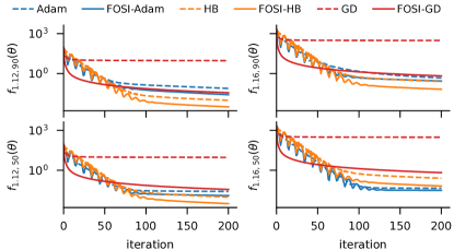
Figure 7: Learning curves of four specific $f_{b,\zeta}$ functions. Each x mark in Figure 3 is the final value of the corresponding learning curve here, i.e. the value of $f$ at iteration 200.

Figure 7 shows the learning curves of the optimizers for four specific $f_{b,\zeta}$ functions: $f_{1.12,50},f_{1.12,90},f_{1.16,50},f_{1.16,90}$. The black x marks in each sub figure of Figure 3 are the last value of these learning curves. For both functions with $b=1.12$ the learning curves of GD and Heavy-Ball (as well as FOSI with these base optimizers) are identical, as they are only differ by a rotation, and similarly for $b=1.16$. However, for the same $\zeta$, these optimizers convergence is much slower for larges $b$ value. FOSI implicitly reduces the maximal eigenvalue in both functions, but the new two maximal eigenvalues still differ by an order of magnitude, which leads to the differences in FOSI’s performance (as opposed to the first experiment on quadratic functions). Adam is negatively impacted when $\zeta$ is increased. In this experiment. For smaller $\zeta$ values its performance is not impacted by the change in $b$ and it is able to converge to the same value even for functions with larger curvature.

Appendix J Evaluation – Learning Rate and Momentum

In the last experiment on quadratic functions, we use each optimizer to optimize the function $f_{1.12,90}$ multiple times, with different learning rates $\eta\in\{1e-5,10\}$. FOSI-HB and FOSI-GD were run with both $c=1$ (no scaling) and $c=\infty$ (no clipping). We repeated the experiment twice. In the first version we used a fixed momentum parameter 0.9 ($\beta$ for HB and $\beta_{1}$ for Adam). In the second version we find the best momentum parameter $\in[0.7,1)$ for each $\eta$.

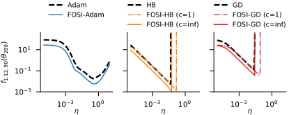
(a) Fixed $\beta$ and $\beta_{1}$ (0.9)

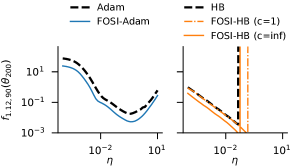
(b) $\beta$ and $\beta_{1}$ tuned per $\eta$

Figure 8: $f_{1.12,90}$ after 200 iterations with different learning rates. Each curve is for a different optimizer, while each point in the curve is the final $f$ value after 200 iterations with a specific learning rate. Left: using a fixed momentum value of 0.9, $\beta$ for HB and $\beta_{1}$ for Adam. Right: the best momentum $\in[0.7,1)$ for each $\eta$. FOSI improves over the base optimizer even when using the optimal hyperparameter set.

Figure 8 shows the results after 200 iterations for every optimizer and learning rate $\eta$. FOSI improves over Adam for all learning rates. For GD and HB, with $c=1$, FOSI expands the range of $\eta$ values for convergence, changes the optimal $\eta$, and leads to superior results after the same number of iterations. With $c=\infty$, FOSI improves over the base optimizer for all $\eta$ values, but the range of $\eta$ values for convergence stays similar. Moreover, FOSI’s improvement over the base optimizer when using the optimal set of hyperparameters is similar to the improvement for a fixed momentum parameters. Similar trends were observed when repeating the experiment for other $f_{b,\zeta}$ functions.

Appendix K Deep Neural Networks – Additional Evaluation Results

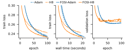
(a) LR

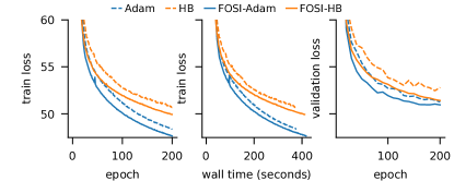
(b) AE

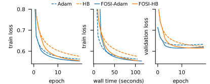
(c) TL

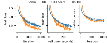
(d) LM

Figure 9: Learning curves of different optimizers for different DNN training tasks. In most cases FOSI obtains faster convergence than the base optimizers across epochs (left) and across wall time (middle). Since FOSI accelerates convergence, it also leads to an earlier overfitting point when the base optimizer has a tendency to overfit, as can be observed in the LR validation loss (right).

Figure 9 shows the learning curves of FOSI and the base optimizers for different DNN training tasks: (1) training logistic regression model on the MNIST dataset, (2) training autoencoder on the CIFAR-10 dataset, (3) transfer learning task in which we train the last layer of trained ResNet-18 on the CIFAR-10 dataset, and (4) training character-level language model with a recurrent network on the Tiny Shakespeare dataset. FOSI improves over the base optimizers in most cases. While FOSI improvement over Adam is less significant than its improvements over Heavy-Ball, there are tasks for which Heavy-Ball performs better than Adam since it generalizes better.

Table 2: Comparison of wall time (in seconds) for each base optimizer and FOSI at the same train loss, which is the minimal train loss of the base Optimizer. A lower wall time is preferable as it indicates the optimizer reaches the best loss at a faster rate.

Task	HB	FOSI-HB	Adam	FOSI-Adam
AC	6845	3599	6042	6825
LM	255	177	255	233
AE	372	322	375	338
TL	103	58	104	71
LR	18	10	19	19

Table 2 shows the time it takes for both the base optimizer and FOSI to reach the same train loss, which is the lowest train loss of the base optimizer. On average, FOSI achieves the same loss over the training set in 78% of the wall time compared to the base optimizers.

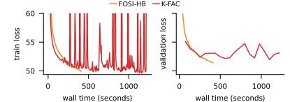
(a) AE

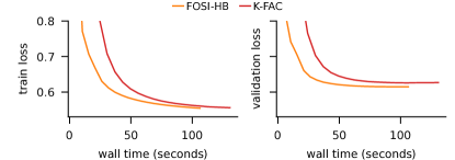
(b) TL

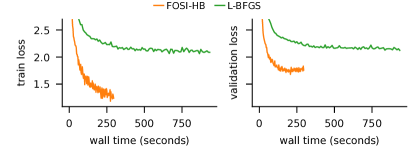
(c) LM

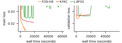
(d) AC

Figure 10: Learning curves of FOSI-BH, K-FAC, and L-BFGS for the DNN training tasks AE, TL, LM, and AC. In the TL figure (top-right), L-BFGS (L=40) was omitted due to its poor performance, resulting in a significantly larger loss than other optimizers and 8x slower wall time. Similarly, in the AE figure (top-left), L-BFGS (L¡=100) was excluded due to its divergence in the first epoch. In the LM figure (bottom-left), K-FAC was omitted due to integration issues with RNN. Across all tasks, FOSI demonstrated faster convergence to a lower validation loss compared to K-FAC and L-BFGS.

Figure 10 shows the learning curves of FOSI-HB, K-FAC and L-BFGS. In all cases, FOSI converges faster and to a lower validation loss than K-FAC and L-BFGS.

References

- Blondel et al. (2021) Blondel, M., Berthet, Q., Cuturi, M., Frostig, R., Hoyer, S., Llinares-López, F., Pedregosa, F., and Vert, J.-P. Efficient and modular implicit differentiation. arXiv preprint arXiv:2105.15183, 2021.
- Botev & Martens (2022) Botev, A. and Martens, J. KFAC-JAX, 2022. URL http://github.com/deepmind/kfac-jax.
- Bradbury et al. (2018) Bradbury, J., Frostig, R., Hawkins, P., Johnson, M. J., Leary, C., Maclaurin, D., Necula, G., Paszke, A., VanderPlas, J., Wanderman-Milne, S., and Zhang, Q. JAX: composable transformations of Python+NumPy programs, 2018. URL http://github.com/google/jax.
- Dorsselaer et al. (2001) Dorsselaer, J., Hochstenbach, M., and Van der Vorst, H. Computing probabilistic bounds for extreme eigenvalues of symmetric matrices with the lanczos method. SIAM Journal on Matrix Analysis and Applications, 22, 01 2001. doi: 10.1137/S0895479800366859.
- Duchi et al. (2011) Duchi, J., Hazan, E., and Singer, Y. Adaptive subgradient methods for online learning and stochastic optimization. J. Mach. Learn. Res., 12(null):2121–2159, jul 2011. ISSN 1532-4435.
- Gallier et al. (2020) Gallier, J. et al. The Schur complement and symmetric positive semidefinite (and definite) matrices (2019). URL https://www. cis. upenn. edu/jean/schur-comp. pdf, 2020.
- Gemmeke et al. (2017) Gemmeke, J. F., Ellis, D. P. W., Freedman, D., Jansen, A., Lawrence, W., Moore, R. C., Plakal, M., and Ritter, M. Audio set: An ontology and human-labeled dataset for audio events. In Proc. IEEE ICASSP 2017, New Orleans, LA, 2017.
- Gentle (2017) Gentle, J. Matrix Algebra: Theory, Computations and Applications in Statistics. Springer, 01 2017. ISBN 978-3-319-64866-8. doi: 10.1007/978-3-319-64867-5.
- Goldfarb et al. (2020) Goldfarb, D., Ren, Y., and Bahamou, A. Practical quasi-newton methods for training deep neural networks. In Proceedings of the 34th International Conference on Neural Information Processing Systems, NIPS’20, Red Hook, NY, USA, 2020. Curran Associates Inc. ISBN 9781713829546.
- Gupta et al. (2018) Gupta, V., Koren, T., and Singer, Y. Shampoo: Preconditioned stochastic tensor optimization. In Dy, J. and Krause, A. (eds.), Proceedings of the 35th International Conference on Machine Learning, volume 80 of Proceedings of Machine Learning Research, pp. 1842–1850. PMLR, 10–15 Jul 2018. URL https://proceedings.mlr.press/v80/gupta18a.html.
- Henriques et al. (2019) Henriques, J. F., Ehrhardt, S., Albanie, S., and Vedaldi, A. Small steps and giant leaps: Minimal Newton solvers for deep learning. In Proceedings of the IEEE/CVF International Conference on Computer Vision, pp. 4763–4772, 2019.
- Karpathy (2015) Karpathy, A. char-rnn, 2015. URL https://github.com/karpathy/char-rnn.
- Kingma & Ba (2014) Kingma, D. and Ba, J. Adam: A method for stochastic optimization. International Conference on Learning Representations, 12 2014.
- Lanczos (1950) Lanczos, C. An iteration method for the solution of the eigenvalue problem of linear differential and integral operators. Journal of research of the National Bureau of Standards, 45:255–282, 1950.
- Lessard et al. (2016) Lessard, L., Recht, B., and Packard, A. Analysis and design of optimization algorithms via integral quadratic constraints. SIAM Journal on Optimization, 26(1):57–95, 2016. doi: 10.1137/15M1009597. URL https://doi.org/10.1137/15M1009597.
- Levy & Duchi (2019) Levy, D. and Duchi, J. C. Necessary and sufficient geometries for gradient methods. Advances in Neural Information Processing Systems, 32, 2019.
- Li (2017) Li, X.-L. Preconditioned stochastic gradient descent. IEEE transactions on neural networks and learning systems, 29(5):1454–1466, 2017.
- Liu & Nocedal (1989) Liu, D. C. and Nocedal, J. On the limited memory BFGS method for large scale optimization. Mathematical programming, 45(1):503–528, 1989.
- Martens & Grosse (2015) Martens, J. and Grosse, R. Optimizing neural networks with Kronecker-factored approximate curvature. In Proceedings of the 32nd International Conference on International Conference on Machine Learning - Volume 37, ICML’15, pp. 2408–2417. JMLR.org, 2015.
- Martens et al. (2018) Martens, J., Ba, J., and Johnson, M. Kronecker-factored curvature approximations for recurrent neural networks. In International Conference on Learning Representations, 2018.
- Meurant & Strakoš (2006) Meurant, G. and Strakoš, Z. The Lanczos and conjugate gradient algorithms in finite precision arithmetic. Acta Numerica, 15:471–542, 2006.
- Nesterov (2003) Nesterov, Y. Introductory lectures on convex optimization: A basic course, volume 87. Springer Science & Business Media, 2003.
- Nocedal & Wright (1999) Nocedal, J. and Wright, S. J. Numerical optimization. Springer, 1999.
- Orvieto et al. (2022) Orvieto, A., Kohler, J., Pavllo, D., Hofmann, T., and Lucchi, A. Vanishing curvature in randomly initialized deep ReLU networks. In Camps-Valls, G., Ruiz, F. J. R., and Valera, I. (eds.), Proceedings of The 25th International Conference on Artificial Intelligence and Statistics, volume 151 of Proceedings of Machine Learning Research, pp. 7942–7975. PMLR, 28–30 Mar 2022. URL https://proceedings.mlr.press/v151/orvieto22a.html.
- Pauloski et al. (2021) Pauloski, J. G., Huang, Q., Huang, L., Venkataraman, S., Chard, K., Foster, I., and Zhang, Z. KAISA: An adaptive second-order optimizer framework for deep neural networks. In Proceedings of the International Conference for High Performance Computing, Networking, Storage and Analysis, SC ’21, New York, NY, USA, 2021. Association for Computing Machinery. ISBN 9781450384421. doi: 10.1145/3458817.3476152. URL https://doi.org/10.1145/3458817.3476152.
- Pearlmutter (1994) Pearlmutter, B. A. Fast exact multiplication by the Hessian. Neural Computation, 6(1):147–160, 1994. doi: 10.1162/neco.1994.6.1.147.
- Polyak (1987) Polyak, B. T. Introduction to optimization. optimization software. Inc., Publications Division, New York, 1:32, 1987.
- Qian (1999) Qian, N. On the momentum term in gradient descent learning algorithms. Neural networks, 12(1):145–151, 1999.
- Qu et al. (2020) Qu, Z., Ye, Y., and Zhou, Z. Diagonal preconditioning: Theory and algorithms. arXiv preprint arXiv:2003.07545, 2020.
- Roosta-Khorasani & Mahoney (2019) Roosta-Khorasani, F. and Mahoney, M. W. Sub-sampled newton methods. Math. Program., 174(1–2):293–326, mar 2019. ISSN 0025-5610. doi: 10.1007/s10107-018-1346-5. URL https://doi.org/10.1007/s10107-018-1346-5.
- Sun & Spall (2021) Sun, S. and Spall, J. C. Connection of diagonal Hessian estimates to natural gradients in stochastic optimization. In 2021 55th Annual Conference on Information Sciences and Systems (CISS), pp. 1–6, 2021. doi: 10.1109/CISS50987.2021.9400243.
- Tan & Lim (2019) Tan, H. H. and Lim, K. H. Review of second-order optimization techniques in artificial neural networks backpropagation. IOP Conference Series: Materials Science and Engineering, 495:012003, jun 2019. doi: 10.1088/1757-899x/495/1/012003. URL https://doi.org/10.1088/1757-899x/495/1/012003.
- Tieleman et al. (2012) Tieleman, T., Hinton, G., et al. Lecture 6.5-rmsprop: Divide the gradient by a running average of its recent magnitude. COURSERA: Neural networks for machine learning, 4(2):26–31, 2012.
- Urschel (2021) Urschel, J. C. Uniform error estimates for the Lanczos method. SIAM Journal on Matrix Analysis and Applications, 42(3):1423–1450, 2021. doi: 10.1137/20M1331470. URL https://doi.org/10.1137/20M1331470.
- Wang et al. (2017) Wang, X., Ma, S., Goldfarb, D., and Liu, W. Stochastic quasi-newton methods for nonconvex stochastic optimization. SIAM Journal on Optimization, 27(2):927–956, 2017. doi: 10.1137/15M1053141. URL https://doi.org/10.1137/15M1053141.
- Wilson et al. (2017) Wilson, A. C., Roelofs, R., Stern, M., Srebro, N., and Recht, B. The marginal value of adaptive gradient methods in machine learning. Advances in neural information processing systems, 30, 2017.
- Xu et al. (2016) Xu, P., Yang, J., Roosta-Khorasani, F., Ré, C., and Mahoney, M. W. Sub-sampled newton methods with non-uniform sampling. In Proceedings of the 30th International Conference on Neural Information Processing Systems, NIPS’16, pp. 3008–3016, Red Hook, NY, USA, 2016. Curran Associates Inc. ISBN 9781510838819.
- Zhou et al. (2020) Zhou, P., Feng, J., Ma, C., Xiong, C., Hoi, S. C. H., et al. Towards theoretically understanding why SGD generalizes better than Adam in deep learning. Advances in Neural Information Processing Systems, 33:21285–21296, 2020.
- Zupanski (2002) Zupanski, M. A preconditioning algorithm for large‐scale minimization problems. Tellus A, 45:478 – 492, 11 2002. doi: 10.1034/j.1600-0870.1993.00011.x.