ST-MFNet Mini: Knowledge Distillation-Driven Frame Interpolation

Abstract

Currently, one of the major challenges in deep learning-based video frame interpolation (VFI) is the large model size and high computational complexity associated with many high performance VFI approaches. In this paper, we present a distillation-based two-stage workflow for obtaining compressed VFI models which perform competitively compared to the state of the art, but with significantly reduced model size and complexity. Specifically, an optimisation-based network pruning method is applied to a state of the art frame interpolation model, ST-MFNet, which suffers from large model size. The resulting network architecture achieves a 91% reduction in parameter numbers and a 35% increase in speed. The performance of the new network is further enhanced through a teacher-student knowledge distillation training process using a Laplacian distillation loss. The final low complexity model, ST-MFNet Mini, achieves a comparable performance to most existing high-complexity VFI methods, only outperformed by the original ST-MFNet. Our source code is available at https://github.com/crispianm/ST-MFNet-Mini

Index Terms—  Video frame interpolation, model compression, knowledge distillation

1 Introduction

Video frame interpolation (VFI) is a widely used technique for increasing the temporal resolution of video content. Recently, deep learning algorithms have enabled a significant boost in the performance of VFI methods [1], and these have been employed extensively in various applications, including video compression, slow motion content rendering and view synthesis [2].

Existing works on VFI generally rely on deep neural networks (DNNs) and can be classified as flow-based or kernel-based. While flow-based VFI methods [3, 4, 5] estimate the optical flow to perform frame warping, kernel-based methods [6, 7, 8] predict per-pixel interpolation kernels to synthesise the target frame. Recent advances in both classes include the use of coarse-to-fine architectures [9, 10], multi-stage/branch pipelines [11, 12, 2, 13], 3D convolution [14, 15], and self-attention mechanisms [16, 17]. Although these latest developments have improved performance on commonly used benchmarks, there has been a tendency to adopt increasingly complex network designs, resulting in large model sizes and higher computational complexity. For example, the recently proposed model ST-MFNet [2] contains 21 million parameters, takes approximately 82MB to store in FP32 (32 bit floating point precision) and requires much longer runtime than much simpler VFI approaches (e.g., 45$\times$ compared to AdaCoF [7]). Such a large model is inefficient in both training and inference (thus having high carbon footprint [18]), imposing high memory requirements and restricting deployment in real-world scenarios.

In order to tackle the problem of large model sizes and high complexity, techniques such as model pruning [19] and knowledge distillation [20] are commonly utilised. One of the few efforts made to apply these to VFI is by Ding et al. [21], pruning the AdaCoF model [7] using a sparsity-inducing optimisation objective [22] to obtain a small network with evidently decreased performance. Newly designed model components were then integrated into this small model to enhance its performance. It is noted that, although a large compression ratio was achieved by pruning the model, the additional components that contributed to the performance gain of the pruned model doubled its size.

In this work, we leverage knowledge distillation to achieve model compression for VFI. This allows a compact model to obtain favourable performance against the state of the arts, without including any additional modules. Specifically, we design a two-stage pipeline (illustrated in Figure 1) to compress ST-MFNet - a recent state-of-the-art VFI model. In the first stage, we follow [21], adopting a sparsity-induced model pruning technique, OBProx-SG [22], to obtain a new, compact ST-MFNet with 91% reduction in the number of parameters. In the second stage, we train using a novel knowledge distillation loss so that it ‘learns’ additional information from the ‘teacher’ model (a pre-trained original ST-MFNet). The resulting low complexity VFI approach, ST-MFNet Mini, outperforms its ‘teacher’ in certain cases, with significantly reduced model size and complexity. To the best of our knowledge, this is the first attempt that employs knowledge distillation for the purpose of model compression in VFI. The proposed framework can potentially be applied to other VFI methods to reduce their model complexity.

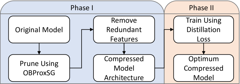
Fig. 1: The proposed VFI compression workflow. Phase I: model size and complexity reduction. Phase II: interpolation performance enhancement.

2 Proposed Method

In this work, we configure the model as in [2]; given four consecutive frames $\{I_{0},I_{1},I_{2},I_{3}\}$, the VFI method outputs $I_{t}$ where $t=1.5$ to achieve $\times$2 interpolation. In this section, we first describe the ST-MFNet architecture and the process of pruning it (Phase I in Figure 1), followed by the knowledge distillation process used to train the compact ST-MFNet (ST-MFNet Mini).

2.1 Pruning ST-MFNet

Given four input frames, the original ST-MFNet first processes these in two branches: MIFNet and BLFNet. While the former uses a U-Net style model to predict per-pixel deformable interpolation kernels, the latter employs a pre-trained optical flow estimator to obtain one-to-one pixel correspondence. These estimated kernels and optical flows are then used to synthesise the target middle frame. The results are passed to a GridNet [23], from which we obtain an intermediate interpolation result, $\tilde{I}_{t}$. This is combined with all four input frames and fed to a 3D CNN to estimate the textural residuals, denoted as $R$. The final output is the combination of these terms, $\tilde{I}_{t}+R$. Readers are referred to [2] for further details.

Sparsity inducing optimisation. In order to obtain a condensed version of ST-MFNet, we start with the original pre-trained model, which is publicly available here, and fine-tune it using the following loss function,

$$\mathcal{L}_{\mathrm{Charb}}(I_{pred},I_{gt})=\sqrt{(I_{pred}-I_{gt})^{2}+\epsilon^{2}},$$ (1)

$$\mathcal{L}_{\mathrm{prune}}=\mathcal{L}_{\mathrm{Charb}}(I_{pred},I_{gt})+\lambda\left\lVert\theta\right\rVert_{1}$$ (2)

where $I_{gt}$ and $I_{pred}$ are the ground-truth target frame and the prediction of ST-MFNet respectively, and $\epsilon=0.001$. The parameters of ST-MFNet are denoted as $\theta$, and $\left\lVert\theta\right\rVert_{1}$ refers to the $l_{1}$ norm regularisation term, which induces sparsity in the network [22]. Such sparsity information can be used as a guide to remove redundant layers in the network. We adopt the OBProx-SG [22] solver to perform the optimisation, which has been shown to be efficient for sparsity-based model pruning [21].

Similarly to [21], we define each layer, $l$, in the model as $l=[C_{out},C_{in},q_{0},q_{1},q_{2}]$, with total number of parameters $p_{l}=C_{out}\cdot C_{in}\cdot q_{0}\cdot q_{1}\cdot q_{2}$. As training takes place, we calculate the density ($d$) for each layer $l$ using

$$d_{l}=\frac{\text{\# of nonzero weights in }l}{p_{l}},$$ (3)

and use these values to compute the average density in the model as an indicator for the training progress. Following [21], we set $\lambda=10^{-4}$ and optimise the network for 20 epochs using our combined training set (Sec. 3.1), achieving a density of approximately 0.24.

Network compression. The sparsity-inducing optimisation described above allows us to identify, through the final layer densities, the individual network layers which contribute less to the overall model performance, and thus can be removed or shrunk. Therefore, starting with the final layer, we use its density as its compression ratio ($r_{n}$), forming a new layer in the form

$$l_{n}^{\prime}=[C_{out},r_{n}\cdot C_{in},q_{0},q_{1},q_{2}],$$

and causing

$$l_{n-1}^{\prime}=[r_{n-1}\cdot C_{out},C_{in},q_{0},q_{1},q_{2}].$$

We iterate through the model’s $n$ layers in this fashiopn, as in [24], ensuring that each layer’s outputs match the previously compressed layer’s inputs.

For ST-MFNet, we found that the flow estimator component of the model (BLFNet) has near-zero compression ratios, so it is removed entirely instead of shrunk. Ultimately, this process prunes the model from 21.03M parameters to 1.82M, a 91% reduction. The architecture of the pruned network (ST-MFNet Mini) is shown in Figure 2

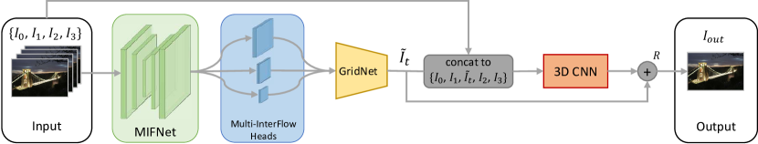
Fig. 2: The resulting model architecture of ST-MFNet Mini.

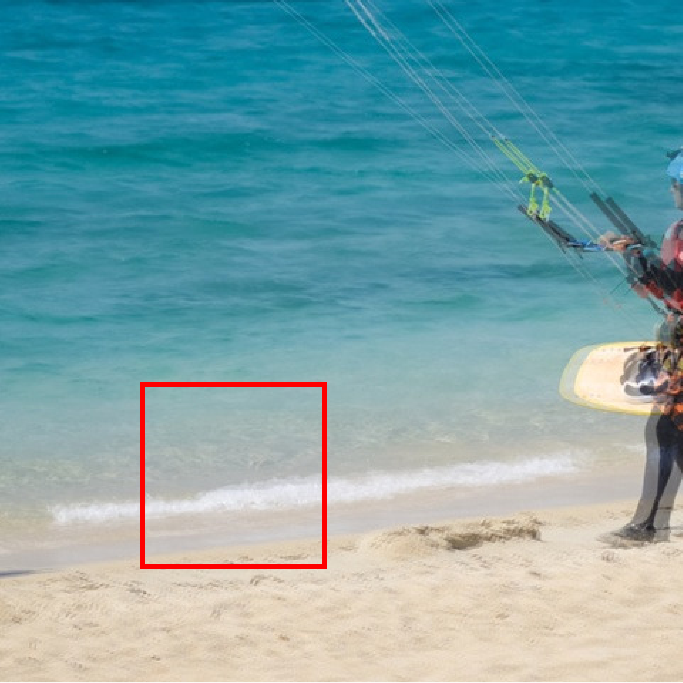
(a) Overlay

(b) ST-MFNet

(c) Ours

(d) GT

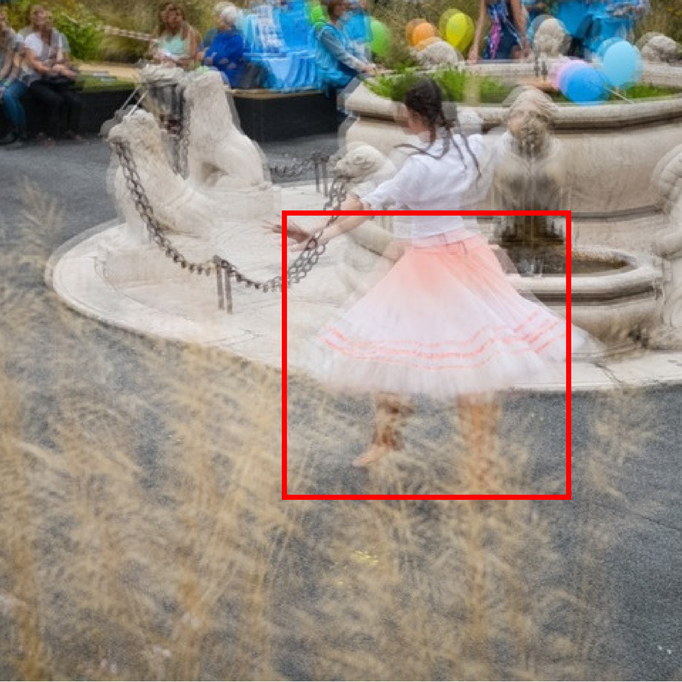
(e) Overlay

(f) ST-MFNet

(g) Ours

(h) GT

​​  ​​  ​​  ​​  ​​  ​​  ​​

Fig. 3: Qualitative examples from the DAVIS test set demonstrating the superiority and shortcomings of our approach.

2.2 Knowledge Distillation

To verify the effectiveness of the distillation loss, a ‘baseline’ model was created by training the pruned model (obtained from the previous stage) on the ground-truth data using a Laplacian loss (the same training conditions as ST-MFNet). We note that, after 20 epochs, this baseline shows decreased average performance compared to the original model (shown in Table 1 in Sec. 3).

In order to enhance the performance of the pruned model, previous approaches [21] have added new components to the model, at the cost of increased model size. In contrast here, we devise a knowledge distillation loss for VFI, where the pruned ‘student’ network learns additional information from the pre-trained original ST-MFNet, the ‘teacher’ network, without any increase in size.

Specifically, the loss function used to train the student network consists of two components. Firstly, the loss between the ground truth and the student model’s prediction ($\mathcal{L}_{stud}$), and secondly, the loss between the student and the teacher’s predictions ($\mathcal{L}_{dist}$). The total loss for the model is therefore

$$\mathcal{L}_{total}=\alpha\mathcal{L}_{stud}(I_{out},I_{gt})+\mathcal{L}_{dist}(I_{pred},I_{out}),$$ (4)

where $I_{gt}$ represents the ground truth frame, $I_{out}$ represents the student model’s output, and $I_{pred}$ represents the original model’s prediction. Here, $\alpha$ is a hyper-parameter controlling the penalty from the ground-truth frames. The student network is trained from scratch using the loss function (Eqn. 4), enabling the pruned network to make use of the additional knowledge learned by the teacher network in prior training.

3 Results and Discussion

3.1 Experimental Setup

Implementation details. The student model is trained for 20 epochs on the same training set as the pre-trained teacher model, i.e. approximately 92K frame quintuplets, from the Vimeo90K septuplet [25] and BVI-DVC [26] datasets. We use Laplacian pyramid loss as both $\mathcal{L}_{stud}$ and $\mathcal{L}_{dist}$, and AdaMax [27] with $\beta_{1}=0.9,\beta_{2}=0.999$. The hyper-parameter $\alpha$ in Eqn. 4 is set to 0.1, based on empirical results.

Evaluation. The model has been evaluated on multiple commonly used test datasets, including UCF101, DAVIS, and SNU-Film. Two commonly used metrics, PSNR and SSIM [28], are used to evaluate the frame interpolation performance.

3.2 Alternative Loss Functions

The baseline and Laplacian distilled models are compared in Table 1, where it can be observed that the distillation process significantly improves model performance. To investigate potential further improvements, particularly in terms of perceptual quality, several GAN-based loss functions were tested as the distillation loss. Specifically, the following adversarial functions were evaluated: GAN [29], ST-GAN [30], and FIGAN [7]. These were trained for 10 epochs on the same training set, with the same hyperparameters as before, and scored respective PSNR values of 32.718, 32.716, and 32.803 on UCF101. Since they failed to improve on the effectiveness of the Laplacian distillation, they were not trained further.

3.3 Qualitative Evaluation

Visual comparisons. Examples of frames interpolated using our model and ST-MFNet are shown in Figure 3. Under certain conditions, the new model’s performance is observably closer to the ground truth than that of ST-MFNet, as evidenced by the first example, while for footage containing large movements, such as for the second case, the model’s performance suffers slightly.

3.4 Quantitative Evaluation

Table 1: Quantitative comparison results (PSNR/SSIM) for ST-MFNet Mini and 13 otjher tested methods. In some cases, scores found using pre-trained models are provided, underlined, when they outperform their re-trained counterparts. For each column, the best result is bold in red and the second best is italicised in blue. The average runtime (RT) for interpolating a 480p DAVIS frame as well as the number of model parameters (#P) for each method are also reported.

	UCF101	DAVIS	SNU-FILM				RT (sec)	#P (M)
			Easy	Medium	Hard	Extreme
SuperSloMo [3]	32.547/0.968	26.523/0.866	36.255/0.984	33.802/0.973	29.519/0.930	24.770/0.855	0.107	39.61
SepConv [6]	32.524/0.968	26.441/0.853	39.894/0.990	35.264/0.976	29.620/0.926	24.653/0.851	0.062	21.68
DAIN [11]	32.524/0.968	27.086/0.873	39.280/0.989	34.993/0.976	29.752/0.929	24.819/0.850	0.896	24.03
BMBC [31]	32.729/0.969	26.835/0.869	39.809/0.990	35.437/0.978	29.942/0.933	24.715/0.856	1.425	11.01
AdaCoF [7]	32.610/0.968	26.445/0.854	39.912/0.990	35.269/0.977	29.723/0.928	24.656/0.851	0.051	21.84
CDFI [21]	32.653/0.968	26.471/0.857	39.881/0.990	35.224/0.977	29.660/0.929	24.645/0.854	0.321	4.98
CAIN [8]	32.537/0.968	26.477/0.857	39.890/0.990	35.630/0.978	29.998/0.931	25.060/0.857	0.071	42.78
SoftSplat [5]	32.835/0.969	27.582/0.881	40.165/0.991	36.017/0.979	30.604/0.937	25.436/0.864	0.206	12.46
EDSC [32]	32.677/0.969	26.689/0.860	39.792/0.990	35.283/0.977	29.815/0.929	24.872/0.854	0.067	8.95
XVFI [33]	32.224/0.966	26.565/0.863	38.849/0.989	34.497/0.975	29.381/0.929	24.677/0.855	0.108	5.61
QVI [4]	32.668/0.967	27.483/0.883	36.648/0.985	34.637/0.978	30.614/0.947	25.426/0.866	0.257	29.23
FLAVR [14]	33.389/0.971	27.450/0.873	40.135/0.990	35.988/0.979	30.541/0.937	25.188/0.860	0.695	42.06
ST-MFNet [2]	33.384/0.970	28.287/0.895	40.775/0.992	37.111/0.985	31.698/0.951	25.810/0.874	0.901	21.03
ST-MFNet Mini (Baseline)	33.013/0.968	26.013/0.848	40.826/0.991	35.858/0.980	30.724/0.946	25.726/0.891	0.588	1.82
ST-MFNet Mini (KD Loss)	33.070/0.969	26.335/0.855	40.982/0.992	36.127/0.982	30.914/0.950	25.877/0.894	0.588	1.82

The quantitative evaluation results are summarised in Table 1. It is noted that the KD-trained compressed model (ST-MFNet Mini) outperforms it’s teacher on two databases: SNU-FILM Easy and Extreme, while its performance on databases with large motions are not as good compared to the state of the art. This may be explained by the fact that the BLFNet component of the model was removed, which was previously shown to improve the model’s ability to handle large motions [2].

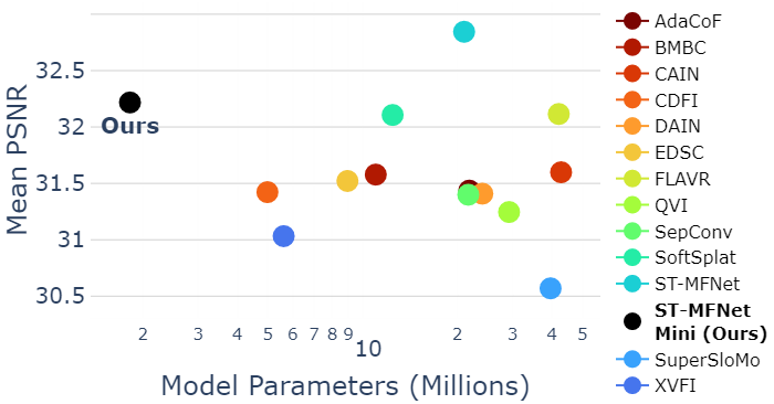
Fig. 4: Mean PSNR scores from the models presented in Table 1. On average, our method outperforms all models except its teacher, at a greatly reduced size.

Figure 4 plots the mean PSNR values of all the tested VFI approaches against their model parameters. It can be observed that STMFNet Mini achieves an excellent trade off between performance and model size, with the lowest model size but second best overall performance. The model with the second fewest model parameters, CDFI, is nearly three times as large.

However, while the compressed model outperforms for its size, it does not meet the same expectations for its runtime. Despite being 35% faster than the original ST-MFNet, the model is still significantly slower than other, larger models. This is most likely due to the upscaling component of ST-MFNet (3D CNN), which requires lengthy computation time; it will be a focus of our future work.

4 Conclusion

A workflow for frame interpolation model compression is presented which utilises model pruning to determine a reduced model architecture and knowledge distillation to improve its performance. When applied to an advanced VFI approach, ST-MFNet; the resulting low complexity model (ST-MFNet Mini) only requires 9% of the original model’s parameters to achieve competitive interpolation performance compared to the state-of-the-art. Future work should focus on generalising this workflow to other VFI approaches, employing more effective knowledge distillation implementations (e.g., feature based) during training in the second stage and on approaches that significantly reduce model runtime.

References

- [1] J. Dong, K. Ota, and M. Dong, “Video Frame Interpolation: A Comprehensive Survey,” ACM Transactions on Multimedia Computing, Communications and Applications, 2022.
- [2] D. Danier, F. Zhang, and D. Bull, “ST-MFNet: A spatio-temporal multi-flow network for frame interpolation,” in Proceedings of the IEEE/CVF Conference on Computer Vision and Pattern Recognition, 2022, pp. 3521–3531.
- [3] H. Jiang, D. Sun, V. Jampani, M.-H. Yang, E. Learned-Miller, and J. Kautz, “Super slomo: High quality estimation of multiple intermediate frames for video interpolation,” in Proceedings of the IEEE Conference on Computer Vision and Pattern Recognition, 2018, pp. 9000–9008.
- [4] X. Xu, L. Siyao, W. Sun, Q. Yin, and M.-H. Yang, “Quadratic video interpolation,” in NeurIPS, 2019.
- [5] S. Niklaus and F. Liu, “Softmax splatting for video frame interpolation,” in Proceedings of the IEEE/CVF Conference on Computer Vision and Pattern Recognition, 2020, pp. 5437–5446.
- [6] S. Niklaus, L. Mai, and F. Liu, “Video frame interpolation via adaptive separable convolution,” in Proceedings of the IEEE International Conference on Computer Vision, 2017, pp. 261–270.
- [7] H. Lee, T. Kim, T.-y. Chung, D. Pak, Y. Ban, and S. Lee, “Adacof: Adaptive collaboration of flows for video frame interpolation,” in Proceedings of the IEEE/CVF Conference on Computer Vision and Pattern Recognition, 2020, pp. 5316–5325.
- [8] M. Choi, H. Kim, B. Han, N. Xu, and K. M. Lee, “Channel attention is all you need for video frame interpolation,” in Proceedings of the AAAI Conference on Artificial Intelligence, vol. 34, 2020, pp. 10 663–10 671.
- [9] F. Reda, J. Kontkanen, E. Tabellion, D. Sun, C. Pantofaru, and B. Curless, “FILM: Frame interpolation for large motion,” in Computer Vision–ECCV 2022: 17th European Conference, Tel Aviv, Israel, October 23–27, 2022, Proceedings, Part VII. Springer, 2022, pp. 250–266.
- [10] L. Kong, B. Jiang, D. Luo, W. Chu, X. Huang, Y. Tai, C. Wang, and J. Yang, “Ifrnet: Intermediate feature refine network for efficient frame interpolation,” in Proceedings of the IEEE/CVF Conference on Computer Vision and Pattern Recognition, 2022, pp. 1969–1978.
- [11] W. Bao, W.-S. Lai, C. Ma, X. Zhang, Z. Gao, and M.-H. Yang, “Depth-aware video frame interpolation,” in Proceedings of the IEEE/CVF Conference on Computer Vision and Pattern Recognition, 2019, pp. 3703–3712.
- [12] W. Bao, W.-S. Lai, X. Zhang, Z. Gao, and M.-H. Yang, “Memc-net: Motion estimation and motion compensation driven neural network for video interpolation and enhancement,” IEEE transactions on pattern analysis and machine intelligence, vol. 43, no. 3, pp. 933–948, 2019.
- [13] S. Gui, C. Wang, Q. Chen, and D. Tao, “Featureflow: Robust video interpolation via structure-to-texture generation,” in Proceedings of the IEEE/CVF Conference on Computer Vision and Pattern Recognition, 2020, pp. 14 004–14 013.
- [14] T. Kalluri, D. Pathak, M. Chandraker, and D. Tran, “Flavr: Flow-agnostic video representations for fast frame interpolation,” arXiv preprint arXiv:2012.08512, 2020.
- [15] D. Danier, F. Zhang, and D. Bull, “Enhancing deformable convolution based video frame interpolation with coarse-to-fine 3d cnn,” in 2022 IEEE International Conference on Image Processing (ICIP). IEEE, 2022, pp. 1396–1400.
- [16] L. Lu, R. Wu, H. Lin, J. Lu, and J. Jia, “Video frame interpolation with transformer,” in Proceedings of the IEEE/CVF Conference on Computer Vision and Pattern Recognition, 2022, pp. 3532–3542.
- [17] Z. Shi, X. Xu, X. Liu, J. Chen, and M.-H. Yang, “Video frame interpolation transformer,” in Proceedings of the IEEE/CVF Conference on Computer Vision and Pattern Recognition, 2022, pp. 17 482–17 491.
- [18] A. Lacoste, A. Luccioni, V. Schmidt, and T. Dandres, “Quantifying the carbon emissions of machine learning,” arXiv preprint arXiv:1910.09700, 2019.
- [19] R. Reed, “Pruning algorithms-a survey,” IEEE transactions on Neural Networks, vol. 4, no. 5, pp. 740–747, 1993.
- [20] G. Hinton, O. Vinyals, and J. Dean, “Distilling the knowledge in a neural network,” arXiv preprint arXiv:1503.02531, 2015.
- [21] T. Ding, L. Liang, Z. Zhu, and I. Zharkov, “CDFI: Compression-driven network design for frame interpolation,” in Proceedings of the IEEE/CVF Conference on Computer Vision and Pattern Recognition, 2021, pp. 8001–8011.
- [22] T. Chen, T. Ding, B. Ji, G. Wang, Y. Shi, J. Tian, S. Yi, X. Tu, and Z. Zhu, “Orthant based proximal stochastic gradient method for -regularized optimization,” in Machine Learning and Knowledge Discovery in Databases: European Conference, ECML PKDD 2020, Ghent, Belgium, September 14–18, 2020, Proceedings, Part III. Springer, 2021, pp. 57–73.
- [23] D. Fourure, R. Emonet, E. Fromont, D. Muselet, A. Tremeau, and C. Wolf, “Residual conv-deconv grid network for semantic segmentation,” arXiv preprint arXiv:1707.07958, 2017.
- [24] T. Chen, B. Ji, Y. Shi, T. Ding, B. Fang, S. Yi, and X. Tu, “Neural network compression via sparse optimization,” arXiv preprint arXiv:2011.04868, 2020.
- [25] T. Xue, B. Chen, J. Wu, D. Wei, and W. T. Freeman, “Video enhancement with task-oriented flow,” International Journal of Computer Vision, vol. 127, no. 8, pp. 1106–1125, 2019.
- [26] D. Ma, F. Zhang, and D. Bull, “BVI-DVC: A training database for deep video compression,” IEEE Transactions on Multimedia, pp. 1–1, 2021.
- [27] D. P. Kingma and J. Ba, “Adam: A method for stochastic optimization,” arXiv preprint arXiv:1412.6980, 2014.
- [28] Z. Wang, A. C. Bovik, H. R. Sheikh, and E. P. Simoncelli, “Image quality assessment: from error visibility to structural similarity,” IEEE transactions on image processing, vol. 13, no. 4, pp. 600–612, 2004.
- [29] I. Goodfellow, J. Pouget-Abadie, M. Mirza, B. Xu, D. Warde-Farley, S. Ozair, A. Courville, and Y. Bengio, “Generative adversarial networks,” Communications of the ACM, vol. 63, no. 11, pp. 139–144, 2020.
- [30] F. Yang, G.-S. Xia, L. Zhang, and X. Huang, “Stationary dynamic texture synthesis using convolutional neural networks,” in 2016 IEEE 13th International Conference on Signal Processing (ICSP). IEEE, 2016, pp. 1135–1139.
- [31] J. Park, K. Ko, C. Lee, and C.-S. Kim, “BMBC: Bilateral motion estimation with bilateral cost volume for video interpolation,” in Computer Vision–ECCV 2020: 16th European Conference, Glasgow, UK, August 23–28, 2020, Proceedings, Part XIV 16. Springer, 2020, pp. 109–125.
- [32] X. Cheng and Z. Chen, “Multiple video frame interpolation via enhanced deformable separable convolution,” IEEE Transactions on Pattern Analysis and Machine Intelligence, 2021.
- [33] H. Sim, J. Oh, and M. Kim, “XVFI: extreme video frame interpolation,” in Proceedings of the IEEE International Conference on Computer Vision (ICCV), 2021.