AirGNNs: Graph Neural Networks over the Air

Abstract

Graph neural networks (GNNs) are information processing architectures that model representations from networked data and allow for decentralized implementation through localized communications. Existing GNN architectures often assume ideal communication links and ignore channel effects, such as fading and noise, leading to performance degradation in real-world implementation. This paper proposes graph neural networks over the air (AirGNNs), a novel GNN architecture that incorporates the communication model into the architecture. AirGNN modifies the graph convolutional operation that shifts graph signals over random communication graphs to take into account channel fading and noise when aggregating features from neighbors, thus, improving the architecture robustness to channel impairments during testing. We propose a stochastic gradient descent based method to train the AirGNN, and show that the training procedure converges to a stationary solution. Numerical simulations on decentralized source localization and multi-robot flocking corroborate theoretical findings and show superior performance of the AirGNN over wireless communication channels.

I Introduction

Graph neural networks (GNNs) are one of the key tools to extract features from networked data [1, 2, 3, 4], and have found wide applications in wireless communications [5, 6], multi-agent coordination [7, 8, 9] and recommendation systems [10, 11, 12]. GNNs extend conventional convolutional neural networks (CNNs) to graph structures by employing a multi-layered architecture with each layer comprising a graph filter bank and a pointwise nonlinearity [13]. With the distributed nature of graph filters, GNNs can compute output features with local neighborhood information. This makes GNNs suitable candidates for decentralized implementation, where each node takes actions by only sensing its local environment and communicating with its neighboring nodes [14, 15].

On the other hand, when implemented in a decentralized fashion, information exchanges among neighboring nodes of GNNs require wireless transmissions. Existing works often assume ideal communications and ignore channel impairments, such as fading and noise, which affect all wireless transmissions [16, 17, 18]. In real-world wireless networks, each node receives faded/noisy messages from its neighbors and computes its output that mismatches the one assuming ideal communications during training; hence, resulting in performance degradation during testing. The work in [19] studied the privacy-preserving problem in decentralized implementation of GNNs over wireless communication channels and used channel state information (CSI) to design signaling strategies for privacy enhancement, while [20] considered the decentralized power allocation problem and estimated CSI to generate transmitted power with GNNs. However, these works require CSI to design signaling strategies for decentralized implementation, which may be inaccurate or unavailable, and focus on specific problems, which are not applicable for general decentralized tasks. In addition, they apply the message passing mechanism of GNNs based on direct adjacencies, i.e., immediate neighbors, without higher-order/multi-hop information.

This paper proposes the AirGNN which incorporates wireless communication channels directly into the GNN architecture. This is inspired by [21], which showed that incorporating channel noise into training can make deep neural networks more robust when network parameters are delivered over noisy communication channels. The AirGNN accounts for channel fading effects and Gaussian noise among the nodes of a GNN during training, where each node generates features based on faded/noisy neighborhood information from multi-hop communications. This yields the learned parameters robust to wireless channel impairments during implementation and improves performance in decentralized tasks without requiring CSI to modulate signals. Our contributions are summarized as follows:

1. We develop the AirGNN framework as a multi-layered architecture where each layer consists of graph filters over the air (AirGFs) and a pointwise nonlinearity (Sec. II). The AirGF shifts graph signals over wireless communication channels in an uncoded fashion to collect multi-hop neighborhood information and generates higher-level features by aggregating faded/noisy information. These features are passed to the nonlinearity and subsequently to successive layers to generate the output of the AirGNN.

2. We formulate the cost function with respect to (w.r.t.) channel fading effects and Gaussian noise, and develop a stochastic gradient descent (SGD) based method to train the AirGNN (Sec. III). We show that this training procedure is equivalent to solving an associated stochastic optimization problem with SGD and prove its convergence to a stationary solution at a rate proportional to the inverse square root of the number of iterations (Sec. IV).

3. We evaluate AirGNNs numerically on the decentralized tasks of source localization and multi-robot flocking to corroborate theoretical findings, and show that they consistently outperform the conventional GNN implemented over noisy communication channels, i.e., when channel effects are ignored during training (Sec. V).

II GNNs over the Air (AirGNNs)

Let $\mathcal{G}=(\mathcal{V},\mathcal{E})$ be a graph with node set $\mathcal{V}=\{1,\cdots,n\}$ and edge set ${\mathcal{E}}$. The graph structure can be represented by an $n\times n$ matrix ${\mathbf{S}}$, referred to as the graph shift operator, with $(i,j)$th entry $[{\mathbf{S}}]_{ij}=s_{ij}$ non-zero only if node $j$ is connected to node $i$, i.e., $(j,i)\in\mathcal{E}$, or $i=j$, such as the adjacency matrix ${\mathbf{A}}$ and the Laplacian matrix ${\mathbf{L}}$ [22]. The graph signal is a vector defined on the nodes ${\mathbf{x}}=[x_{1},\ldots,x_{n}]^{\top}$, where the $i$th entry $x_{i}$ is the signal value associated to node $i$. The graph serves as a mathematical representation of the network topology and the graph signal captures the network states. For example, in a multi-agent system, nodes can correspond to agents, edges to communication links, and signal values to agent states.

The graph shift operation ${\mathbf{S}}{\mathbf{x}}$ is one of the key operations in graph signal processing. It assigns to each node $i$ the aggregated information from its neighboring nodes $[{\mathbf{x}}^{(1)}]_{i}=[{\mathbf{S}}{\mathbf{x}}]_{i}$ and extends the signal shifting from the time/space domain to the graph domain. In the context of real-world networked systems (e.g., sensor networks and multi-agent systems), this corresponds to message exchanges between the neighboring sensors/agents over available communications links. However, ${\mathbf{S}}{\mathbf{x}}$ assumes perfect signal transmissions between nodes and ignores the fact that communication links suffer from channel fading and additive noise in practice.

Communication channel. We assume that each node exchanges information wirelessly with the neighboring nodes in its communication range. The channel between the nodes $i$ and $j$ is modeled as a slow fading channel, the signal value $[{\mathbf{x}}]_{j}$ is transmitted in an uncoded/analog manner, and the neighborhood information is aggregated at node $i$ with over-the-air computation, i.e.,

$$[{\mathbf{x}}^{(1)}]_{i}\!=\!\sum_{j:(i,j)\in{\mathcal{E}}}\!h_{ij}^{(1)}[{\mathbf{x}}]_{j}+n_{i}^{(1)},\leavevmode\nobreak\ \text{for}\leavevmode\nobreak\ i=1,...,n,$$ (1)

where $h^{(1)}_{ij}$ is the channel gain from node $j$ to node $i$ and $n_{i}^{(1)}$ is the zero-mean Gaussian noise at node $i$. The channel fading effects $\{h_{ij}\}$ are assumed independent across communication links, which are fixed throughout a single transmission but changes from one transmission to the next in an independent and identically distributed (i.i.d.) manner. Hence, each node receives noisy and faded versions of the messages sent by its neighbors, and the graph shift operation becomes

$${\mathbf{x}}^{(1)}={\mathbf{S}}_{\rm air}^{(1)}{\mathbf{x}}+{\mathbf{n}}^{(1)},$$ (2)

where ${\mathbf{S}}^{(1)}_{\rm air}$ is the graph shift operator with channel fading effects, i.e., $[{\mathbf{S}}^{(1)}_{\rm air}]_{ij}=h_{ij}^{(1)}$ for any $(i,j)\in{\mathcal{E}}$, and ${\mathbf{n}}$ is the Gaussian noise vector with $[{\mathbf{n}}]_{i}=n_{i}$ for $i=1,\ldots,n$. Different from its ideal counterpart ${\mathbf{S}}{\mathbf{x}}$, the signal shifting in (2) depends not only on the graph topology, but also on the communication channels, and we refer to the latter as the graph shift operation over the air (AirGSO).

Graph filter over the air (AirGF). AirGF is a linear combination of multi-shifted signals over the air. Specifically, an AirGSO shifts ${\mathbf{x}}$ over ${\mathbf{S}}$ through wireless communication channels and obtains the one-shifted signal ${\mathbf{x}}^{(1)}$ that aggregates $1$-hop neighborhood information [cf. (2)]. By recursively shifting ${\mathbf{x}}$, the $k$-shifted signal ${\mathbf{x}}^{(k)}$ is

$${\mathbf{x}}^{(k)} ={\mathbf{S}}_{\rm air}^{(k)}\Big{(}{\mathbf{S}}_{\rm air}^{(k-1)}\big{(}\cdots+{\mathbf{n}}^{(1)}\big{)}+{\mathbf{n}}^{(k-1)}\Big{)}+{\mathbf{n}}^{(k)}$$ (3)

$$=\prod_{\kappa=1}^{k}{\mathbf{S}}_{\rm air}^{(\kappa)}{\mathbf{x}}+\sum_{i=1}^{k-1}\prod_{\kappa=i+1}^{k}{\mathbf{S}}_{\rm air}^{(\kappa)}{\mathbf{n}}^{(i)}+{\mathbf{n}}^{(k)},$$

where ${\mathbf{S}}_{\rm air}^{(k)}$ and ${\mathbf{n}}^{(k)}$ are, respectively, the AirGSO and Gaussian noise vector at the $k$th graph shift operation. The $k$-shifted signal ${\mathbf{x}}^{(k)}$ accesses farther nodes and aggregates the $k$-hop neighborhood information with communication noise. Given a sequence of shifted signals $\{{\mathbf{x}},{\mathbf{x}}^{(1)},\ldots,{\mathbf{x}}^{(K)}\}$, the AirGF aggregates them with a set of filter coefficients as

$${\mathbf{H}}_{\rm air}({\mathbf{S}}){\mathbf{x}}=\sum_{k=0}^{K}\alpha_{k}{\mathbf{x}}^{(k)}={\mathbf{P}}_{\rm air}({\mathbf{S}},{\mathbf{x}})+{\mathbf{N}}_{\rm air}({\mathbf{S}},{\mathbf{n}})$$ (4)

$$=\sum_{k=0}^{K}\alpha_{k}\prod_{\kappa=1}^{k}{\mathbf{S}}_{\rm air}^{(\kappa)}{\mathbf{x}}+\sum_{k=1}^{K}\alpha_{k}\left(\sum_{i=1}^{k-1}\prod_{\kappa=i+1}^{k}{\mathbf{S}}_{\rm air}^{(\kappa)}{\mathbf{n}}^{(i)}+{\mathbf{n}}^{(k)}\right),$$

where ${\mathbf{x}}^{(0)}={\mathbf{x}}$ by default and $\boldsymbol{\alpha}=[\alpha_{0},\ldots,\alpha_{K}]^{\top}$ are the filter coefficients. The first term in (4) captures the signal information perturbed by the communication channels, referred to as the signal component, while the second term in (4) is the accumulated noise, referred to as the noise component. The AirGF is a shift-and-sum operator that extends graph convolution to wireless communication channels. It aggregates the neighborhood information up to a radius of $K$ and accounts for channel fading and Gaussian noise when shifting signals over the underlying graph. AirGF reduces to a conventional graph filter in ideal scenarios, where the communication links are perfect, i.e., $h_{ij}^{(1)}=1$ and $n_{i}^{(1)}=0$ in (1).

AirGNN. AirGNN is an information processing architecture that consists of multiple layers, where each layer comprises a bank of AirGFs and a pointwise nonlinearity. Specifically, at layer $\ell$, we have $F$ input signals $\{{\mathbf{x}}_{\ell-1}^{g}\}_{g=1}^{F}$ generated by the previous layer $\ell-1$. The latter are processed by a bank of AirGFs $\{{\mathbf{H}}_{{\rm air},\ell}^{fg}\}_{fg}$, aggregated over the input index $g$, and passed through a pointwise nonlinearity $\sigma(\cdot)$ as

$${\mathbf{x}}_{\ell}^{f}=\sigma\left(\sum_{g=1}^{F}{\mathbf{H}}_{{\rm air},\ell}^{fg}({\mathbf{S}}){\mathbf{x}}_{\ell-1}^{g}\right),\leavevmode\nobreak\ \forall\leavevmode\nobreak\ f=1,\ldots,F.$$ (5)

The outputs $\{{\mathbf{x}}_{\ell}^{f}\}_{f=1}^{F}$ are fed into layer $\ell+1$ until the final layer $L$. Without loss of generality, we consider a single input ${\mathbf{x}}_{0}^{1}={\mathbf{x}}$ and a single output ${\mathbf{x}}_{L}^{1}$. The AirGNN can be represented as a nonlinear mapping $\boldsymbol{\Phi}_{\rm air}({\mathbf{x}},{\mathbf{S}},{\mathcal{A}})$ of graph signals ${\mathbf{x}}$, where ${\mathcal{A}}$ are the architecture parameters comprising all filter coefficients. AirGNN reduces to a conventional GNN if assuming ideal communications without channel fading or noise among the neighboring nodes.

Decentralized implementation. AirGNN and AirGF are ready for decentralized implementation, i.e., each node can compute its own output with local neighborhood information. Specifically, the one-shifted signal $[{\mathbf{x}}^{(1)}]_{i}$ at node $i$ can be computed with signal values $\{[{\mathbf{x}}]_{j}\}_{j:(i,j)\in{\mathcal{E}}}$ at neighboring nodes transmitted through wireless communication links in an uncoded fashion [cf. (1)]. Likewise, $K$ shifted signals $\{[{\mathbf{x}}^{(k)}]_{i}\}_{k=0}^{K}$ at node $i$ can be computed with recursive communications between neighboring nodes. Since the aggregation of the shifted signals $\{[{\mathbf{x}}^{(k)}]_{i}\}_{k=0}^{K}$ with the filter coefficients $\{\alpha_{k}\}_{k=0}^{K}$ does not involve inter-node operations, node $i$ can compute the filter output $[{\mathbf{H}}_{\rm air}({\mathbf{S}}){\mathbf{x}}]_{i}$ locally with neighborhood information and the AirGF allows for a decentralized implementation. AirGNN consists of AirGFs and nonlinearities, where the former is decentralized and the latter is pointwise and local; hence, inheriting the decentralized implementation. This implies that a node does not need signal values of all the nodes and the full knowledge of the graph to compute the AirGNN/AirGF output, but only the ability to communicate local signals in a synchronized manner with their neighbors, in order to allow over-the-air aggregation, similarly to [23, 24].

With the consideration of wireless communication channels, the AirGNN output is a random variable w.r.t. channel state information (CSI) and Gaussian noise [cf. (1)]. It is unclear how to train the AirGNN, whether the training procedure converges to a stationary solution, and what solution it searches for. We address these aspects in the following sections.

III Training

We develop a SGD based method to train the AirGNN. For a specific task with the training set ${\mathcal{R}}=\{({\mathbf{x}}_{r},{\mathbf{y}}_{r})\}_{r=1}^{R}$ and loss function $\ell(\cdot)$, we define the objective function as the expected loss over the training set

$${\mathcal{L}}(\mathcal{R},{\mathbf{S}},{\mathcal{A}})=\frac{1}{R}\sum_{r=1}^{R}\ell({\mathbf{y}}_{r},\boldsymbol{\Phi}_{\rm air}({\mathbf{x}}_{r},{\mathbf{S}},{\mathcal{A}})).$$ (6)

Since the AirGNN output $\boldsymbol{\Phi}_{\rm air}({\mathbf{x}}_{r},{\mathbf{S}},{\mathcal{A}})$ is a random variable, the objective ${\mathcal{L}}(\mathcal{R},{\mathbf{S}},{\mathcal{A}})$ is a random function w.r.t. channel fading effects and Gaussian noise. The goal is to find the optimal architecture parameters ${\mathcal{A}}^{*}$ that minimize the objective function ${\mathcal{L}}(\mathcal{R},{\mathbf{S}},{\mathcal{A}})$ while accounting for channel impairments.

We propose to update ${\mathcal{A}}$ with gradient descent while incorporating the randomness of the communication channels during training. Specifically, let $\boldsymbol{\Phi}_{\rm air}({\mathbf{x}},{\mathbf{S}},{\mathcal{A}}|{\mathbf{h}},{\mathbf{n}})$ be a sample of the AirGNN output on the graph signal ${\mathbf{x}}$, where ${\mathbf{h}}$ and ${\mathbf{n}}$ are samples of the CSI and the Gaussian noise, respectively, throughout graph shift operations of all AirGFs in the architecture. The training procedure contains successive iterations to optimize the objective function, where each iteration $t$ consists of a forward and a backward phase. In the forward phase, it samples the CSI ${\mathbf{h}}_{t}$ and the Gaussian noise ${\mathbf{n}}_{t}$ for a deterministic AirGNN architecture $\boldsymbol{\Phi}_{\rm air}({\mathbf{x}},{\mathbf{S}},{\mathcal{A}}_{t}|{\mathbf{h}}_{t},{\mathbf{n}}_{t})$ with parameters ${\mathcal{A}}_{t}$. The latter processes a random set of the training data ${\mathcal{R}}_{t}\in{\mathcal{R}}$ to approximate the objective function as

$${\mathcal{L}}(\mathcal{R}_{t},\!{\mathbf{S}},\!{\mathcal{A}}_{t}|{\mathbf{h}}_{t},\!{\mathbf{n}}_{t})\!=\!\frac{1}{|{\mathcal{R}}_{t}|}\!\sum_{r=1}^{|{\mathcal{R}}_{t}|}\!\ell({\mathbf{y}}_{r},\boldsymbol{\Phi}_{\rm air}({\mathbf{x}}_{r},\!{\mathbf{S}},\!{\mathcal{A}}_{t}|{\mathbf{h}}_{t},\!{\mathbf{n}}_{t})\big{)},$$ (7)

where $({\mathbf{x}}_{r},{\mathbf{y}}_{r})\in{\mathcal{R}}_{t}$ and $|{\mathcal{R}}_{t}|$ is the number of data samples in set ${\mathcal{R}}_{t}$. In the backward phase, the parameters ${\mathcal{A}}_{t}$ are updated with SGD as

$${\mathcal{A}}_{t+1}={\mathcal{A}}_{t}-\gamma_{t}\nabla_{\mathcal{A}}{\mathcal{L}}(\mathcal{R}_{t},{\mathbf{S}},{\mathcal{A}}_{t}|{\mathbf{h}}_{t},{\mathbf{n}}_{t}),$$ (8)

where $\gamma_{t}$ is the step-size. It accounts for the effects of the communication channels by updating the parameters ${\mathcal{H}}_{t}$ with a stochastic gradient $\nabla_{\mathcal{A}}{\mathcal{L}}(\mathcal{R}_{t},{\mathbf{S}},{\mathcal{A}}_{t}|{\mathbf{h}}_{t},{\mathbf{n}}_{t})$ at each iteration $t$. The stochasticity results from the randomness of the CSI ${\mathbf{h}}_{t}$, the Gaussian noise ${\mathbf{n}}_{t}$, as well as the randomly chosen samples ${\mathcal{R}}_{t}$. Algorithm 1 summarizes the proposed training procedure.

1:Input: training set $\mathcal{R}$, loss function $\ell$, initial parameters ${\mathcal{A}}_{0}$

2:for $t=1,\dots,T$ do

3:     Sample CSI ${\mathbf{h}}_{t}$ and Gaussian noise ${\mathbf{n}}_{t}$

4:     Determine AirGNN architecture $\boldsymbol{\Phi}_{\rm air}(\cdot,{\mathbf{S}},{\mathcal{A}}_{t}|{\mathbf{h}}_{t},{\mathbf{n}}_{t})$

5:     Sample ${\mathcal{R}}_{t}\subseteq{\mathcal{R}}$ and compute AirGNN outputs $\{\boldsymbol{\Phi}_{\rm air}({\mathbf{x}}_{r},{\mathbf{S}},{\mathcal{A}}_{t}|{\mathbf{h}}_{t},{\mathbf{n}}_{t})\}_{r=1}^{|{\mathcal{R}}_{t}|}$

6:     Compute objective ${\mathcal{L}}(\mathcal{R}_{t},{\mathbf{S}},{\mathcal{A}}_{t}|{\mathbf{h}}_{t},{\mathbf{n}}_{t})$ as in (7)

7:     Compute stochastic gradient $\nabla_{\mathcal{A}}{\mathcal{L}}(\mathcal{R}_{t},{\mathbf{S}},{\mathcal{A}}_{t}|{\mathbf{h}}_{t},{\mathbf{n}}_{t})$

8:     Update parameters ${\mathcal{A}}_{t}$ with step-size $\gamma_{t}$ as in (8)

9:end for

Algorithm 1 Training Procedure of AirGNN

AirGNN incorporates communication channel impairments into the training procedure, where each node relies on faded and noisy information from its neighbors [cf. (1)]. This matches the fading and noise distributions encountered in the decentralized implementation at the inference phase and renders the trained parameters more robust to transmission perturbations during testing; hence, yielding an improved performance and a robust transference for decentralized tasks. However, it remains unclear if this training procedure converges and what solution it searches for. In the next section, we conduct the convergence analysis and interpret the convergent solution.

IV Convergence

We begin by considering the following stochastic optimization problem as

$$\min_{{\mathcal{A}}}\bar{{\mathcal{L}}}({\mathcal{A}})=\min_{{\mathcal{A}}}\mathbb{E}_{{\mathbf{h}},{\mathbf{n}}}[{\mathcal{L}}(\mathcal{R},{\mathbf{S}},{\mathcal{A}}|{\mathbf{h}},{\mathbf{n}})],$$ (9)

where the expectation $\mathbb{E}_{{\mathbf{h}},{\mathbf{n}}}[\cdot]$ is w.r.t. ${\mathbf{h}}$ and ${\mathbf{n}}$. The standard method to solve problem (9) is the SGD, which approximates the true gradient with the gradient of some random sample and leverages the latter to update model parameters – see Algorithm 2. Theorem 1 relates the proposed training procedure to this stochastic optimization problem (9).

Theorem 1.

Performing the proposed training procedure on the AirGNN model [Alg. 1] is equivalent to running SGD on the stochastic optimization problem (9) [Alg. 2].

Proof.

See Appendix A. ∎

Theorem 1 provides interpretations for the proposed training procedure, i.e., its goal is to search the solution of the stochastic optimization problem (9). Moreover, the result indicates that we can show the convergence of the proposed training procedure by proving that of the SGD on problem (9). Since AirGNN is a nonlinear parameterization, problem (9) is typically non-convex. This motivates us to consider the convergence criterion as the gradient norm $\|\nabla_{\mathcal{A}}\bar{{\mathcal{L}}}({\mathcal{A}})\|^{2}_{2}$, which is commonly used to quantify the first-order stationarity in the non-convex setting. To proceed, we need the following assumptions.

Assumption 1.

The gradient of the expected objective function $\bar{{\mathcal{L}}}({\mathcal{A}})$ in problem (9) is Lipschitz continuous, i.e., there exists a constant $C_{L}$ such that

$$\begin{split}\|\nabla_{\mathcal{A}}\bar{{\mathcal{L}}}({\mathcal{A}}_{1})-\nabla_{\mathcal{A}}\bar{{\mathcal{L}}}({\mathcal{A}}_{2})\|_{2}\leq C_{L}\|{\mathcal{A}}_{1}-{\mathcal{A}}_{2}\|_{2}\end{split}$$ (10)

for any architecture parameters ${\mathcal{A}}_{1}$ and ${\mathcal{A}}_{2}$.

Assumption 2.

The gradient of the objective function ${\mathcal{L}}(\mathcal{R},{\mathbf{S}},{\mathcal{A}}|{\mathbf{h}},{\mathbf{n}})$ in problem (9) is bounded, i.e., there exists a constant $C_{g}$ such that

$$\begin{split}\|\nabla_{\mathcal{A}}{\mathcal{L}}(\mathcal{R},{\mathbf{S}},{\mathcal{A}}|{\mathbf{h}},{\mathbf{n}})\|_{2}\leq C_{g}.\end{split}$$ (11)

Assumptions 1-2 are standard in optimization theory [25], which provide a handle to deal with the gradient stochasticity during training. Theorem 2 characterizes the convergence of the proposed training procedure.

1:Input: training set $\mathcal{R}$, loss function $\ell$, initial parameters ${\mathcal{A}}_{0}$

2:Set batch-size of training data ${\mathcal{R}}$ as $|{\mathcal{R}}_{t}|$ and batch-size of communication channels $({\mathbf{h}},{\mathbf{n}})$ as $1$

3:for $t=1,\dots,T$ do

4:     Sample a random objective function ${\mathcal{L}}(\mathcal{R}_{t},{\mathbf{S}},{\mathcal{A}}_{t}|{\mathbf{h}}_{t},{\mathbf{n}}_{t})$ [cf. (7)]

5:     Compute stochastic gradient $\nabla_{\mathcal{A}}{\mathcal{L}}(\mathcal{R}_{t},{\mathbf{S}},{\mathcal{A}}_{t}|{\mathbf{h}}_{t},{\mathbf{n}}_{t})$

6:     Update model parameters with step-size $\gamma_{t}$ as ${\mathcal{A}}_{t+1}={\mathcal{A}}_{t}-\gamma_{t}\nabla_{\mathcal{A}}{\mathcal{L}}(\mathcal{R}_{t},{\mathbf{S}},{\mathcal{A}}_{t}|{\mathbf{h}}_{t},{\mathbf{n}}_{t})$

7:end for

Algorithm 2 SGD for Problem (9)

Theorem 2.

Consider the AirGNN operation in (5) with the training procedure in Algorithm 1 and the stochastic optimization problem (9) with the objective function satisfying Assumptions 1-2 w.r.t. $C_{L}$ and $C_{g}$. Let $T$ be the total number of training iterations and ${\mathcal{A}}^{*}$ the global optimal solution of problem (9). Then, for any initial parameters ${\mathcal{A}}_{0}$ and the step-size

$$\begin{split}\gamma_{t}=\gamma=\sqrt{\frac{2\left(\bar{{\mathcal{L}}}({\mathcal{A}}_{0})-\bar{{\mathcal{L}}}({\mathcal{A}}^{*})\right)}{TC_{L}C_{g}^{2}}},\end{split}$$ (12)

it holds that

$$\begin{split}\min_{0\leq t\leq T-1}\mathbb{E}\left[\|\nabla_{\mathcal{A}}\bar{{\mathcal{L}}}({\mathcal{A}}_{t})\|^{2}_{2}\right]\leq\frac{C}{\sqrt{T}}\end{split}$$ (13)

with $C\!=\!\sqrt{2\left(\bar{{\mathcal{L}}}({\mathcal{A}}_{0})\!-\!\bar{{\mathcal{L}}}({\mathcal{A}}^{*})\right)C_{L}}C_{g}$ a constant.

Proof.

See Appendix B. ∎

Theorem 2 states that the proposed AirGNN training procedure minimizes the stochastic optimization problem (9) and the architecture parameters converge to a stationary solution with a rate on the order of ${\mathcal{O}}(1/\sqrt{T})$. The result characterizes the convergence behavior and validates the effectiveness of the proposed training procedure. The selection of the step-size $\gamma_{t}$ in (12) depends on the total number of iterations $T$, while it is typically selected as $\gamma_{t}\propto 1/t$ or $1/\sqrt{t}$ in practice. It is worth mentioning that Theorem 2 guarantees local convergence because of the non-convexity, i.e., the objective function converges to a local stationary minimum rather than a global one. The latter can be improved by training the AirGNN architecture multiple times and selecting the best solution.

V Experiments

We evaluate AirGNN on the decentralized tasks of source localization (Sec. V-A) and multi-robot flocking (Sec. V-B). The ADAM optimizer is used with decaying factors $\beta_{1}=0.9$, $\beta_{2}=0.999$ [26] and the results are averaged over $10$ simulations.

V-A Source Localization

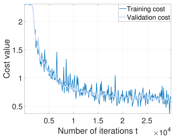
(a)

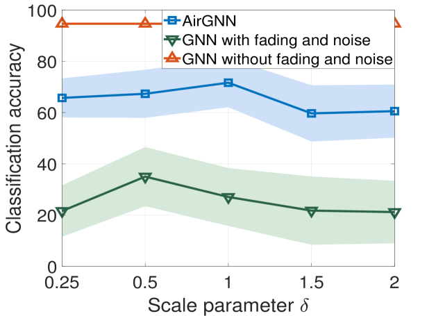
(b)

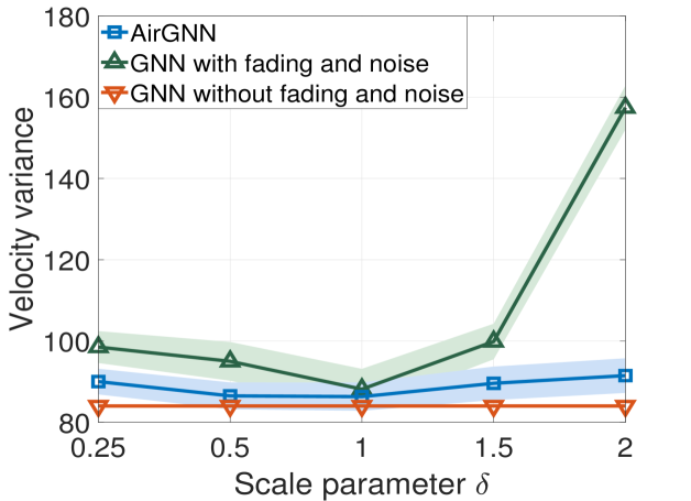
(c)

Figure 1: (a) Training procedure of the AirGNN with $\delta=1$. (b) Source localization: Performance of the AirGNN and baselines in different channel conditions, i.e., different $\delta$. (c) Multi-robot flocking: Performance of the AirGNN and baselines in different channel conditions, i.e., different $\delta$.

This experiment considers a signal diffusion process over a stochastic block model (SBM) graph, where the intra- and the inter-community edge probabilities are $0.8$ and $0.2$. The graph has $n=100$ nodes uniformly divided into $10$ communities and each community has a source node $s_{c}$ for $c=1,\ldots,10$. The goal is to find the source community of a diffused signal in a decentralized manner. The initial signal is a Kronecker delta $\boldsymbol{\delta}_{c}\in{\mathbb{R}}^{n}$ originated at one of the source nodes $\{s_{c}\}_{c=1}^{10}$ and is diffused over the graph at time $\tau$ as ${\mathbf{x}}_{c,\tau}={\mathbf{S}}^{\tau}\boldsymbol{\delta}_{c}+{\mathbf{n}}$ with ${\mathbf{S}}={\mathbf{A}}/\lambda_{max}({\mathbf{A}})$ and ${\mathbf{n}}$ a zero-mean Gaussian noise. The dataset consists of $1.5\times 10^{4}$ samples with the source node $s_{c}$ and the diffusion time $\tau$ selected randomly from $\{s_{1},\ldots,s_{10}\}$ and $\{1,\ldots,100\}$, which are split into $10^{4}$ samples for training, $2.5\times 10^{3}$ for validation, and $2.5\times 10^{3}$ for testing. The AirGNN has two layers, each comprising $64$ filters of order $5$ and ReLU nonlinearity. We consider independent Rayleigh fading channels between the nodes with distribution scale parameter $\delta$ and the Gaussian noise with signal-to-noise ratio (SNR) $40$dB. The learning rate is set to $10^{-3}$, the batch-size to $50$, and the performance is measured in terms of the classification accuracy.

Fig. 1(a) shows the training procedure of the AirGNN with the scale parameter $\delta=1$. We see that the training/validation cost decreases with the iteration and approaches a stationary solution, which corroborates the convergence analysis in Theorem 2. The convergence curve fluctuates, because the channel fading effects and mini-batch sampling render the AirGNN output random.

Fig. 1(b) depicts the performance of the AirGNN with different scale parameters $\delta$ corresponding to different channel conditions. We compare with two baselines: (i) GNN without channel fading and noise, and (ii) GNN with channel fading and noise. The first considers a classical GNN with no fading and noise, i.e., $h_{ij}^{(k)}=1$ and $n_{i}^{(k)}=0$ for $k=1,\ldots,K$ [cf. (1)], during both training and inference. This is an ideal communication scenario, which may not hold in real-world wireless applications and serves as an upper bound only for reference. The second considers fading and noise during inference, which is the practical scenario considered in this paper, but ignores them during training. The GNN without fading and noise exhibits the best performance as expected as it does not consider any channel effects. The AirGNN consistently outperforms the GNN with fading and noise. This corroborates the theoretical analysis, i.e., the AirGNN accounts for the stochasticity of the communication channels during training, which provides robustness to channel fading effects during inference. Moreover, the AirGNN maintains a good performance in different channel conditions, while the GNN suffers more degradation in severe channels when $\delta$ is small or large. The latter highlights the importance of robustness to communication noise.

V-B Multi-Robot Flocking

This experiment considers the robot swarm control over the communication graph. The goal is to learn a decentralized controller that coordinates the robots to move together and avoid collision. The network has $n=50$ robots with initial velocities sampled randomly in $[-3m/s,3m/s]^{2}$, and robot $i$ can communicate with robot $j$ if they are within a communication radius of $r=1.5m$. The communication graph is ${\mathcal{G}}=({\mathcal{V}},{\mathcal{E}})$ with the node set ${\mathcal{V}}$ as the robots and the edge set ${\mathcal{E}}$ as available communication links, and the graph signal ${\mathbf{x}}$ is the relevant features of robot positions and velocities. We use imitation learning to train the AirGNN by mimicing the optimal centralized controller [7]. The dataset consists of $450$ trajectories of $100$ time steps, which are split into $400$ trajectories for training, $25$ for validation, and $25$ for testing. We consider a single-layer AirGNN with $32$ filters of order $5$ and the hyperbolic tangent nonlinearity. The learning rate is $5\times 10^{-4}$ and the batch-size is $20$. We measure the performance with the variance of robot velocities for a trajectory, which quantifies how far from the consensus the robots are.

Fig. 1(c) compares the performance of the AirGNN with two baselines in different channel conditions. The AirGNN performs comparably to the GNN without fading and noise with slight degradation. This is because the information loss induced by channel impairments leads to inevitable errors, which cannot be resolved completely by training. The AirGNN exhibits a better performance compared to the GNN with fading and noise, which is particularly significant for small or large values of $\delta$, i.e., worse channel conditions. We attribute this behavior to the robustness of the AirGNN to fading effects because it accounts for communication channels during training.

VI Conclusion

We proposed AirGNNs in order to improve architecture robustness to wireless channel impairments for decentralized implementation of GNNs. AirGNNs consist of multiple layers with each layer comprising graph filters over the air and a pointwise nonlinearity. They incorporate communication channels into graph signal processing and leverage noisy neighborhood information to extract features, which alleviate the performance degradation caused by channel fading and noise. We account for random channel states in the cost function and developed a SGD based method for training AirGNNs. We showed the proposed training procedure is equivalent to running SGD on an associated stochastic optimization problem and proved its convergence to a stationary solution. Numerical experiments are performed on decentralized tasks of source localization and multi-robot flocking, corroborating the effectiveness of AirGNNs to improve the performance over communication channels.

A. Proof of Theorem 1

Proof.

The objective function ${\mathcal{L}}(\mathcal{R},{\mathbf{S}},{\mathcal{A}}|{\mathbf{h}},{\mathbf{n}})$ is determined by the AirGNN architecture, which is, in turn, determined by the channel fading ${\mathbf{h}}$, the Gaussian noise ${\mathbf{n}}$ and the data ${\mathcal{R}}$. This indicates that sampling an objective function ${\mathcal{L}}(\mathcal{R}_{t},{\mathbf{S}},{\mathcal{A}}_{t}|{\mathbf{h}}_{t},{\mathbf{n}}_{t})$ is equivalent to sampling an AirGNN architecture $\boldsymbol{\Phi}_{\rm air}(\cdot,{\mathbf{S}},{\mathcal{A}}|{\mathbf{h}}_{t},{\mathbf{n}}_{t})$, i.e., sampling ${\mathbf{h}}_{t}$, ${\mathbf{n}}_{t}$ and ${\mathcal{R}}_{t}$. By leveraging this observation and comparing Algorithms 1-2, steps $3$-$6$ in the proposed training procedure [Alg. 1] is equivalent to step $4$ in the SGD on problem (9) [Alg. 2]. Since the other steps are the same, we conclude that the proposed training procedure of the AirGNN is equivalent to the SGD on problem (9) with the training data batch-size $R_{t}$ and the communication channel batch-size $1$. ∎

B. Proof of Theorem 2

Proof.

By using the Taylor expansion of $\mathbb{E}\left[\bar{{\mathcal{L}}}({\mathcal{A}}_{t+1})\right]$ at ${\mathcal{H}}_{t}$, we can represent $\mathbb{E}\left[\bar{{\mathcal{L}}}({\mathcal{A}}_{t+1})\right]$ as

$$\mathbb{E}\!\left[\bar{{\mathcal{L}}}({\mathcal{A}}_{t\!+\!1})\right]\!=\!\mathbb{E}\!\left[\bar{{\mathcal{L}}}({\mathcal{A}}_{t})\right.\!+\!\nabla_{\mathcal{A}}\bar{{\mathcal{L}}}({\mathcal{A}}_{t})^{\top}\!\left({\mathcal{A}}_{t+1}-{\mathcal{A}}_{t}\right)$$ (14)

$$\leavevmode\nobreak\ \leavevmode\nobreak\ \leavevmode\nobreak\ \leavevmode\nobreak\ \leavevmode\nobreak\ \leavevmode\nobreak\ \leavevmode\nobreak\ \leavevmode\nobreak\ \leavevmode\nobreak\ \leavevmode\nobreak\ \leavevmode\nobreak\ \leavevmode\nobreak\ \leavevmode\nobreak\ \leavevmode\nobreak\ +\frac{1}{2}\left({\mathcal{A}}_{t+1}\!-\!{\mathcal{A}}_{t}\right)^{\top}\nabla^{2}_{\mathcal{A}}\bar{{\mathcal{L}}}(\tilde{{\mathcal{A}}}_{t})\left({\mathcal{A}}_{t+1}-{\mathcal{A}}_{t}\right)\big{]}\!$$

where $\tilde{{\mathcal{A}}}_{t}$ is in the line segment joining ${\mathcal{A}}_{t+1}$ and ${\mathcal{A}}_{t}$, which truncates the expansion series at the Hessian term. From the fact that ${\mathbf{v}}^{\top}{\mathbf{M}}{\mathbf{v}}\leq\lambda_{\max}({\mathbf{M}})\|{\mathbf{v}}\|_{2}^{2}$ for any vector ${\mathbf{v}}$ and matrix ${\mathbf{M}}$ with $\lambda_{\max}({\mathbf{M}})$ the maximal eigenvalue of ${\mathbf{M}}$ and the Lipschitz continuity $\|\nabla^{2}_{\mathcal{A}}\bar{{\mathcal{L}}}(\tilde{{\mathcal{A}}}_{t})\|_{2}\leq C_{L}$ of Assumption 1, we have

$$\mathbb{E}\!\left[\bar{{\mathcal{L}}}({\mathcal{A}}_{t+1})\right]$$ (15)

$$\leq\mathbb{E}\big{[}\bar{{\mathcal{L}}}({\mathcal{A}}_{t})\!+\!\nabla_{\mathcal{A}}\bar{{\mathcal{L}}}({\mathcal{A}}_{t})^{\top}({\mathcal{A}}_{t+1}\!-\!{\mathcal{A}}_{t})\!+\!\frac{C_{L}}{2}\!\|{\mathcal{A}}_{t+1}\!-\!{\mathcal{A}}_{t}\|_{2}^{2}\big{]}.$$

Substituting the update rule of the AirGNN ${\mathcal{A}}_{t+1}={\mathcal{A}}_{t}-\gamma_{t}\nabla_{\mathcal{A}}{\mathcal{L}}({\mathcal{R}}_{t},{\mathbf{S}},{\mathcal{A}}_{t}|{\mathbf{h}}_{t},{\mathbf{n}}_{t})$ into (15) yields

$$\mathbb{E}\!\left[\bar{{\mathcal{L}}}({\mathcal{A}}_{t+1})\right]\! \leq\mathbb{E}\big{[}\bar{{\mathcal{L}}}({\mathcal{A}}_{t})+\frac{\gamma_{t}^{2}C_{L}}{2}\|\nabla_{\mathcal{A}}{\mathcal{L}}({\mathcal{R}}_{t},{\mathbf{S}},{\mathcal{A}}_{t}|{\mathbf{h}}_{t},{\mathbf{n}}_{t})\|_{2}^{2}$$

$$-\gamma_{t}\nabla_{\mathcal{A}}\bar{{\mathcal{L}}}({\mathcal{A}}_{t})^{\top}\nabla_{\mathcal{A}}{\mathcal{L}}({\mathcal{R}}_{t},{\mathbf{S}},{\mathcal{A}}_{t}|{\mathbf{h}}_{t},{\mathbf{n}}_{t})\big{]}.$$ (16)

By using the linearity of expectation and the identity $\mathbb{E}[\nabla_{\mathcal{A}}{\mathcal{L}}({\mathcal{R}}_{t},{\mathbf{S}},{\mathcal{A}}_{t}|{\mathbf{h}}_{t},{\mathbf{n}}_{t})]=\mathbb{E}[\nabla_{\mathcal{A}}\bar{{\mathcal{L}}}({\mathcal{A}}_{t})]$, we can re-write (Proof.) as

$$\mathbb{E}\left[\bar{{\mathcal{L}}}({\mathcal{A}}_{t+1})\right] \leq\mathbb{E}\big{[}\bar{{\mathcal{L}}}({\mathcal{A}}_{t})]-\gamma_{t}\mathbb{E}\big{[}\|\nabla_{\mathcal{A}}\bar{{\mathcal{L}}}({\mathcal{A}}_{t})\|_{2}^{2}\big{]}$$ (17)

$$+\frac{\gamma_{t}^{2}C_{L}}{2}\mathbb{E}\big{[}\|\nabla_{\mathcal{A}}{\mathcal{L}}({\mathcal{R}}_{t},{\mathbf{S}},{\mathcal{A}}_{t}|{\mathbf{h}}_{t},{\mathbf{n}}_{t})\|_{2}^{2}\big{]}.$$

From the gradient bound of Assumption 2, we can upper bound the third term of (17) as

$$\begin{split}\frac{\gamma_{t}^{2}C_{L}}{2}\mathbb{E}\big{[}\|\nabla_{\mathcal{A}}{\mathcal{L}}({\mathcal{R}}_{t},{\mathbf{S}},{\mathcal{A}}_{t}|{\mathbf{h}}_{t},{\mathbf{n}}_{t})\|_{2}^{2}\big{]}\leq\frac{\gamma_{t}^{2}C_{L}C_{g}^{2}}{2}.\end{split}$$ (18)

By substituting (18) into (17), we have

$$\begin{split}\mathbb{E}[\|\nabla_{\mathcal{A}}\bar{{\mathcal{L}}}({\mathcal{A}}_{t})\|_{2}^{2}]\leq\frac{1}{\gamma_{t}}\mathbb{E}\big{[}\bar{{\mathcal{L}}}({\mathcal{A}}_{t})\!-\!\bar{{\mathcal{L}}}({\mathcal{A}}_{t+1})\big{]}\!+\!\frac{\gamma_{t}C_{L}C_{g}^{2}}{2}.\end{split}$$ (19)

Since (19) holds for all iterations $t=0,\ldots,T-1$, by considering a constant step-size $\gamma_{t}=\gamma$ and summing up (19) over all iterations, we have

$$\sum_{t=0}^{T-1}\mathbb{E}[\|\nabla_{\mathcal{A}}\bar{{\mathcal{L}}}({\mathcal{A}}_{t})\|^{2}]$$ (20)

$$\leq\frac{1}{\gamma}\mathbb{E}\big{[}\bar{{\mathcal{L}}}({\mathcal{A}}_{0})-\bar{{\mathcal{L}}}({\mathcal{A}}_{T})\big{]}+\frac{\gamma TC_{L}C_{g}^{2}}{2}.$$

For the optimal parameters ${\mathcal{A}}^{*}$, we have $\bar{{\mathcal{L}}}({\mathcal{A}}^{*})\!\leq\!\bar{{\mathcal{L}}}({\mathcal{A}}_{T})$. This allows to bound (20) as

$$\min_{t}\mathbb{E}\big{[}\|\nabla_{\mathcal{A}}\bar{{\mathcal{L}}}({\mathcal{A}}_{t})\|^{2}\big{]}\leq\frac{1}{T}\sum_{t=0}^{T-1}\mathbb{E}\big{[}\|\nabla_{\mathcal{A}}\bar{{\mathcal{L}}}({\mathcal{A}}_{t})\|^{2}\big{]}$$

$$\leq\frac{1}{T\gamma}\left(\bar{{\mathcal{L}}}({\mathcal{A}}_{0})-\bar{{\mathcal{L}}}({\mathcal{A}}^{*})\right)+\frac{\gamma C_{L}C_{g}^{2}}{2}.$$ (21)

By further setting the constant step-size as

$$\begin{split}\gamma\!=\!\sqrt{\frac{2\left(\bar{{\mathcal{L}}}({\mathcal{A}}_{0})-\bar{{\mathcal{L}}}({\mathcal{A}}^{*})\right)}{TC_{L}C_{g}^{2}}}\end{split}$$ (22)

and substituting it into (Proof.), we complete the proof

$$\begin{split}&\min_{t}\mathbb{E}[\|\nabla_{\mathcal{A}}\bar{{\mathcal{L}}}({\mathcal{A}}_{t})\|^{2}]\leq\frac{C}{\sqrt{T}}\end{split}$$ (23)

where $C\!=\!\sqrt{2\!\left(\bar{{\mathcal{L}}}({\mathcal{A}}_{0})-\bar{{\mathcal{L}}}({\mathcal{A}}^{*})\right)\!C_{L}}C_{g}$ is a constant. ∎

References

- [1] F. Scarselli, M. Gori, A. C. Tsoi, M. Hagenbuchner, and G. Monfardini, “The graph neural network model,” IEEE Transactions on Neural Networks, vol. 20, no. 1, pp. 61–80, 2008.
- [2] M. Defferrard, X. Bresson, and P. Vandergheynst, “Convolutional neural networks on graphs with fast localized spectral filtering,” Advances in Neural Information Processing Systems, vol. 29, 2016.
- [3] Z. Gao, E. Isufi, and A. Ribeiro, “Stochastic graph neural networks,” IEEE Transactions on Signal Processing, vol. 69, pp. 4428–4443, 2021.
- [4] K. Xu, W. Hu, J. Leskovec, and S. Jegelka, “How powerful are graph neural networks?,” in International Conference on Learning Representations (ICLR), 2019.
- [5] Z. Gao, M. Eisen, and A. Ribeiro, “Resource allocation via graph neural networks in free space optical fronthaul networks,” in IEEE Global Communications Conference (GLOBECOM), 2020.
- [6] Z. Gao, Y. Shao, D. Gunduz, and A. Prorok, “Decentralized channel management in WLANs with graph neural networks,” arXiv preprint arXiv:2210.16949, 2022.
- [7] E. Tolstaya, F. Gama, J. Paulos, G. Pappas, V. Kumar, and A. Ribeiro, “Learning decentralized controllers for robot swarms with graph neural networks,” in Conference on Robot Learning (CoRL), 2020.
- [8] Z. Gao and A. Prorok, “Environment optimization for multi-agent navigation,” arXiv preprint arXiv:2209.11279, 2022.
- [9] S. Chen, J. Dong, P. Ha, Y. Li, and S. Labi, “Graph neural network and reinforcement learning for multi-agent cooperative control of connected autonomous vehicles,” Computer-Aided Civil and Infrastructure Engineering, vol. 36, no. 7, pp. 838–857, 2021.
- [10] R. Ying, R. He, K. Chen, P. Eksombatchai, W. L. Hamilton, and J. Leskovec, “Graph convolutional neural networks for web-scale recommender systems,” in ACM SIGKDD International Conference on Knowledge Discovery & Data Mining, 2018.
- [11] Z. Gao and E. Isufi, “Learning stochastic graph neural networks with constrained variance,” IEEE Transactions on Signal Processing, vol. 71, pp. 358–371, 2023.
- [12] Shu Wu, Yuyuan Tang, Yanqiao Zhu, Liang Wang, Xing Xie, and Tieniu Tan, “Session-based recommendation with graph neural networks,” in AAAI Conference on Artificial Intelligence, 2019.
- [13] F. Gama, A. G. Marques, G. Leus, and A. Ribeiro, “Convolutional neural network architectures for signals supported on graphs,” IEEE Transactions on Signal Processing, vol. 67, no. 4, pp. 1034–1049, 2018.
- [14] F. Gama, Q. Li, E. Tolstaya, A. Prorok, and A. Ribeiro, “Synthesizing decentralized controllers with graph neural networks and imitation learning,” IEEE Transactions on Signal Processing, vol. 70, pp. 1932–1946, 2022.
- [15] Z. Gao, F. Gama, and A. Ribeiro, “Wide and deep graph neural network with distributed online learning,” IEEE Transactions on Signal Processing, vol. 70, pp. 3862–3877, 2022.
- [16] F. Belloni, “Fading models,” Postgraduate Course in Radio Communications, pp. 1–4, 2004.
- [17] K. P. Peppas, H. E. Nistazakis, and G. S. Tombras, “An overview of the physical insight and the various performance metrics of fading channels in wireless communication systems,” Advanced Trends in Wireless Communications, pp. 1–22, 2011.
- [18] S. Popa, N. Draghiciu, and R. Reiz, “Fading types in wireless communications systems,” Journal of Electrical and Electronics Engineering, vol. 1, no. 1, pp. 233–237, 2008.
- [19] M. Lee, G. Yu, and H. Dai, “Privacy-preserving decentralized inference with graph neural networks in wireless networks,” arXiv preprint arXiv:2208.06963, 2022.
- [20] Y. Gu, C. She, Z. Quan, C. Qiu, and X. Xu, “Distributed graph neural networks for optimizing wireless networks: Message passing over-the-air,” arXiv preprint arXiv:2207.08498, 2022.
- [21] M. Jankowski, D. Gündüz, and K. Mikolajczyk, “Airnet: Neural network transmission over the air,” in IEEE International Symposium on Information Theory (ISIT), 2022.
- [22] A. Sandryhaila and J. M. F. Moura, “Discrete signal processing on graphs,” IEEE Transactions on Signal Processing, vol. 61, no. 7, pp. 1644–1656, 2013.
- [23] M. M. Amiri and D. Gündüz, “Federated learning over wireless fading channels,” IEEE Transactions on Wireless Communications, vol. 19, no. 5, pp. 3546–3557, 2020.
- [24] M. M. Amiri, T. M. Duman, D. Gündüz, S. R. Kulkarni, and H. V. Poor, “Blind federated edge learning,” IEEE Transactions on Wireless Communications, vol. 20, no. 8, pp. 5129–5143, 2021.
- [25] H. T. Jongen, K. Meer, and E. Triesch, Optimization theory, Springer Science & Business Media, 2007.
- [26] D. Kingma and J. Ba, “Adam: A method for stochastic optimization,” in International Conference on Learning Representations (ICLR), 2010.