A Frequency Domain Analysis of Slow Coherency in Networked Systems

Abstract

Network coherence generally refers to the emergence of simple aggregated dynamical behaviours, despite heterogeneity in the dynamics of the subsystems that constitute the network. In this paper, we develop a general frequency domain framework to analyze and quantify the level of network coherence that a system exhibits by relating coherence with a low-rank property of the system’s input-output response. More precisely, for a networked system with linear dynamics and coupling, we show that, as the network’s effective algebraic connectivity grows, the system transfer matrix converges to a rank-one transfer matrix representing the coherent behavior. Interestingly, the non-zero eigenvalue of such a rank-one matrix is given by the harmonic mean of individual nodal dynamics, and we refer to it as the coherent dynamics. Our analysis unveils the frequency-dependent nature of coherence and a non-trivial interplay between dynamics and network topology. We further show that many networked systems can exhibit similar coherent behavior by establishing a concentration result in a setting with randomly chosen individual nodal dynamics.

, ,

1 Introduction

The study of coordinated behavior in network systems has been a popular subject of research in many fields, including physics [2], chemistry [3], social sciences [4], and biology [5]. Within engineering, coordination is essential for the proper operation of many networked systems, including power networks [6, 7], data and sensor networks [8, 9], and autonomous transportation [10, 11, 12, 13]. Among many forms of coordination, coherence refers to the ability of a group of nodes to have a similar dynamic response to some external disturbance [14]. While coherence analysis is useful in understanding the collective behavior of large networks, little do we know about the underlying mechanism that causes such coherent behavior to emerge in various networks.

Classic slow coherency analyses [15, 16, 17, 18, 19] (with applications mostly to power networks) usually consider the second-order electro-mechanical model without damping: $\ddot{x}=-M^{-1}Lx$, where $M$ is the diagonal matrix of machine inertias, and $L$ is the Laplacian matrix whose elements are synchronizing coefficients between pair of machines. The coherency or synchrony [16] (a generalized notion of coherency) is identified by studying the first few slowest eigenmodes (eigenvectors with small eigenvalues) of $M^{-1}L$. The analysis can be carried over to the case of uniform [15] and non-uniform [17] damping. However, such state-space-based analysis is limited to very specific node dynamics (second order) and does not account for more complex dynamics or controllers that are usually present at a node level; e.g., in the power systems literature [20, 21, 22]. Moreover, it is widely known that such coherence is related to strong interconnection among the nodes, such relation is not formally justified in the aforementioned slow coherency analyses.

A vast body of work, triggered by the seminal paper [13], has quantitatively studied the role of the network topology in the emergence of coherence. Examples include, directed [23] and undirected [24] consensus networks, transportation networks [13], and power networks [7, 25, 26, 27]. The key technical approach amounts to quantify the level of coherence by computing the $\mathcal{H}_{2}$-norm of the system for appropriately defined nodal disturbance and performance signals. Broadly speaking, the analysis shows a reciprocal dependence between the performance metrics and the non-zero eigenvalues of the network graph Laplacian, validating the fact that strong network coherence (low $\mathcal{H}_{2}$-norm) results from the high connectivity of the network (large Laplacian eigenvalues). Unfortunately, the analysis strongly relies on a homogeneity [13, 23, 24, 25, 26, 27] or proportionality [7] assumption of the nodal transfer functions, and thus fails to characterize how individual heterogeneous node dynamics affect the overall coherent network response.

1.1 Our contribution

In this paper, we seek to overcome these limitations by formalizing network coherence through a low-rank structure of the system transfer matrix that appears when the network feedback gain is high. This frequency domain analysis provides a deeper characterization of the role of both, network topology and node dynamics, on the coherent behavior of the network. In particular, our results make substantial contributions towards the understanding of coordinated and coherent behavior of network systems in many ways:

• We present a general framework in the frequency domain to analyze the coherence of heterogeneous networks. We show that network coherence emerges as a low-rank structure of the system transfer matrix as we increase the effective algebraic connectivity–a frequency-varying quantity that depends on the network coupling strength and dynamics.

• Our analysis applies to networks with heterogeneous nodal dynamics, and further provides an explicit characterization in the frequency domain of the coherent response to disturbances as the harmonic mean of individual nodal dynamics. Thus, in this way, our results highlight the contribution of individual nodal dynamics to the network’s coherent behavior.

• We formally connect our frequency-domain results with explicit time-domain $L_{\infty}$ bounds on the difference between individual nodal responses and the coherent dynamic response to certain classes of input signals, suggesting that network coherence is a frequency-dependent phenomenon. That is, the ability of nodes to respond coherently depends on the frequency composition of the input disturbance.

• By providing an exact characterization of the network’s coherent dynamics, our analysis can be further applied in settings where only distributional information of the network composition is known. More precisely, we show that the coherent dynamics of tightly-connected networks with possibly random nodal dynamics are well approximated by a deterministic transfer function that only depends on the statistical distribution of node dynamics.

Notably, the problem of characterizing coherent dynamic response is unique to heterogeneous networks since the coherent dynamics for homogeneous networks are exactly equal to the common nodal dynamics. In real applications, however, such as power networks, such characterization is relevant to model reduction [28] and control design [21]. Our analysis provides, in the asymptotic sense, the exact characterization of coherent dynamics that can be used in control design for heterogeneous networks.

1.2 Other related work

Consensus and synchronization: Consensus [4, 11, 12, 13, 23, 29, 30] refers to the ability of the network nodes to asymptotically reach a common value over some quantities of interest. Synchronization [5, 8, 9, 10, 31, 32, 33] refers to the ability of network nodes to follow a commonly defined trajectory. Although for nonlinear systems synchronization is a structurally stable phenomenon, in the linear case [31, 10, 32, 33], synchronization requires the existence of a common internal model that acts as a virtual leader [32, 33]. As such, consensus and synchronization are coordinated behavior generally achieved in steady state, and requires a common internal model for every node. On the contrary, the network can exhibit coherent behavior during transient phase (a formal comparison is presented in Section 4.3), and coherence exists even without a common internal model.

Area aggregation and dynamic equivalents: For a group of nodes that exhibit coherent behavior, one can construct dynamic equivalents [15, 16] that characterize the slow coherence. Finding the dynamic equivalent, or an aggregate model, for interconnected power generators is long standing research subject in power system literature. Previously proposed aggregation model [28, 34, 17, 35, 7], mostly assume first- or second-order generator dynamics, which does not account for more complex dynamics or controllers [20, 21, 22]. Our explicit characterization of coherent dynamics provides a principled way to obtain an aggregate model for general node dynamics.

1.3 Paper organization

The paper is organized as follows. In Section 3 we discuss the network coherence as a low-rank property of the network transfer matrix. In Section 4, we discuss the time-domain implication of such coherence in transfer matrix. In Section 5, the dynamics concentration in large-scale networks is discussed. In Section 6, we apply our analysis to synchronous generator networks. Lastly we conclude with a discussion on future research in Section 7.

Notation: For a vector $x$, $\|x\|=\sqrt{x^{\top}x}$ denotes the $2$-norm of $x$, and for a matrix $A$, $\sigma_{\min}(A)$ denotes the minimum singular value of $A$, $\|A\|$ denotes the spectral norm of $A$. Particularly, if $A$ is real symmetric, we let $\lambda_{i}(A)$ denote the $i$th smallest eigenvalue of $A$. We let $\mathrm{diag}\{x_{i}\}_{i=1}^{n}$ denote a $n\times n$ diagonal matrix with diagonal entries $x_{i}$. We let $I_{n}$ denote the identity matrix of order $n$, $\mathbb{1}$ denote column vector $[1,\cdots,1]^{\top}$, $[n]$ denote the set $\{1,2,\cdots,n\}$ and $\mathbb{N}_{+}$ denote the set of positive integers. Also, we write complex numbers as $a+jb$, where $j=\sqrt{-1}$. We denote $\mathbb{C}$ the field of complex number, and define the following subsets $\mathcal{B}(s_{0},\delta):=\{s\in\mathbb{C}:|s-s_{0}|\leq\delta\}$.

2 Problem Setup

Consider a network consisting of $n$ nodes ($n\geq 2$), indexed by $i\in[n]$ with the block diagram structure in Fig.1. $L$ is the Laplacian matrix of the weighted graph that describes the network interconnection. We further use $f(s)$ to denote the transfer function representing the dynamics of network coupling, and $G(s)=\mathrm{diag}\{g_{i}(s)\}$ to denote the nodal dynamics, with $g_{i}(s),\ i\in[n]$, being an SISO transfer function representing the dynamics of node $i$. Throughout this paper, we assume all $g_{i}(s),\ i=1,\cdots,n$ and $f(s)$ are rational proper transfer functions, and the Laplacian matrix $L$ is real symmetric.

Figure 1: Block diagram of networked dynamical systems

Under this setting, we can compactly express the transfer matrix from the input signal vector $\mathbf{u}$ to the output signal vector $\mathbf{y}$ by

$$T(s) =\;(I_{n}+G(s)f(s)L)^{-1}G(s)$$

$$=\;(I_{n}+\mathrm{diag}\{g_{i}(s)\}f(s)L)^{-1}\mathrm{diag}\{g_{i}(s)\}\,.$$ (1)

Many existing networks can be represented by this structure. For example, for the first-order consensus network [29, 11], $f(s)=1$, and the node dynamics are given by $g_{i}(s)=\frac{1}{s}$. For power networks [26, 7], $f(s)=\frac{1}{s}$, $g_{i}(s)$ are the dynamics of the generators, and $L$ is the Laplacian matrix representing the sensitivity of power injection w.r.t. bus phase angles. Finally, in transportation networks [12, 11], $g_{i}(s)$ represent the vehicle dynamics whereas $f(s)L$ describes local inter-vehicle information transfer.

Since $L$ has an eigendecomposition $L=V\Lambda V^{\top}$ where $V=\left[\frac{\mathbb{1}}{\sqrt{n}},V_{\perp}\right]$, $VV^{\top}=V^{\top}V=I_{n}$, and $\Lambda=\mathrm{diag}\{\lambda_{i}(L)\}$ with $0=\lambda_{1}(L)\leq\lambda_{2}(L)\leq\cdots\leq\lambda_{n}(L)$, we can rewrite $T(s)$ as

$$T(s) =\;(I_{n}+\mathrm{diag}\{g_{i}(s)\}f(s)L)^{-1}\mathrm{diag}\{g_{i}(s)\}$$

$$=\;(\mathrm{diag}\{g^{-1}_{i}(s)\}+f(s)L)^{-1}$$

$$=\;(\mathrm{diag}\{g^{-1}_{i}(s)\}+f(s)V\Lambda V^{\top})^{-1}$$

$$=\;V(V^{\top}\mathrm{diag}\{g^{-1}_{i}(s)\}V+f(s)\Lambda)^{-1}V^{\top}\,.$$ (2)

As we mentioned in the introduction, we are interested in the regime where the closed-loop system $T(s)$ of (1) has a low-rank structure. To gain some insight, we first consider the following simplified example.

2.1 Motivating example: homogeneous network

Suppose $g_{i}(s)$ are homogeneous, i.e., $g_{i}(s)=g(s)$. Then using (2) one can decompose $T(s)$ as follows

$$T(s)\!=\!\frac{1}{n}g(s)\mathbb{1}\mathbb{1}^{\top}\!+V_{\perp}\mathrm{diag}\left\{\frac{1}{g^{-1}(s)\!+\!f(s)\lambda_{i}(L)}\right\}_{i=2}^{n}\!\!\!V_{\perp}^{\top}\,,$$ (3)

where the network dynamics decouple into two terms: 1) the dynamics $\frac{1}{n}g(s)\mathbb{1}\mathbb{1}^{\top}$ that is independent of network topology and corresponds to the coherent behavior of the system; 2) the remaining dynamics that are dependent on the network structure via both, the eigenvalues $\lambda_{i}(L),i=2,\cdots,n$ and the eigenvectors $V_{\perp}$. Notice that $|f(s)\lambda_{2}(L)|\leq|f(s)\lambda_{i}(L)|,i=2,\dots,n$, then $\frac{1}{n}g(s)\mathbb{1}\mathbb{1}^{\top}$ is dominant in $T(s)$ as long as $|f(s)\lambda_{2}(L)|$ (later referred as effective algbraic connectivity), is large enough to make the norm of the second term in (3) sufficiently small. Following such observation, we can find two regimes where the coherent dynamics $\frac{1}{n}g(s)\mathbb{1}\mathbb{1}^{\top}$ is dominant:

1. (High network connectivity) If a compact set $S\subset\mathbb{C}$ contains neither zeros nor poles of $g(s)$, then we have $\lim_{\lambda_{2}(L)\rightarrow\infty}\sup_{s\in S}\left\lVert T(s)-\frac{1}{n}g(s)\mathbb{1}\mathbb{1}^{\top}\right\rVert=0\,.$

2. (High gain in coupling dynamics) If $s_{0}$ is a pole of $f(s)$, and the network is connected, i.e., $\lambda_{2}(L)>0$, then we have $\lim_{s\rightarrow s_{0}}\left\lVert T(s)-\frac{1}{n}g(s)\mathbb{1}\mathbb{1}^{\top}\right\rVert=0\,.$

Such convergence results suggest that if 1) the network has high algebraic connectivity, or 2) our point of interest in frequency domain is close to pole of $f(s)$, the response of the entire system is close to one of $\frac{1}{n}g(s)\mathbb{1}\mathbb{1}^{\top}$. We refer $\frac{1}{n}g(s)\mathbb{1}\mathbb{1}^{\top}$ as the coherent dynamics in the sense that in such system, the inputs are aggregated, and all nodes have exactly the same response to the aggregate input. Therefore, coherence of the network corresponds, in the frequency domain, to the property that the network’s transfer matrix approximately having a particular rank-one structure.

The aforementioned analysis can be extended to the case with proportionality assumption, i.e., $g_{i}(s)=p_{i}g(s)$ for some $g(s)$ and $p_{i}>0,i=1,\cdots,n$, where one can still obtain decoupled dynamics through proper coordinate transformation [7] and the coherent dynamics are again characterized by the common dynamics $g(s)$. However, it is challenging to analyze the transfer matrix $T(s)$ without the proportionality assumption: First, it is unclear whether low-rank structure would even emerge under high network connectivity or high gain in the coupling dynamics; Then most importantly, there is no obvious choice for coherent dynamics, hence characterizing the coherent dynamics is a non-trivial problem unique to heterogeneous networks, and no existing work has shown an explicit characterization.

2.2 Goal of this work

Our work precisely aims at understanding the coherent dynamics of non-proportional heterogeneous networks. We would like to show that even when $g_{i}(s)$ are heterogeneous, similar results as in the motivating example still hold. More precisely, we show that, in Section 3, $T(s)$ converges to a rank-one transfer matrix of the form $\frac{1}{n}\bar{g}(s)\mathbb{1}\mathbb{1}^{\top}$, as the effective algebraic connectivity $|f(s)\lambda_{2}(L)|$ increases. However, unlike the homogeneous node dynamics case where the coherent behavior is driven by $\bar{g}(s)=g(s)$, the coherent dynamics $\bar{g}(s)$ are given by the harmonic mean of $g_{i}(s),i=1,\cdots,n$, i.e.,

$$\bar{g}(s)=\left(\frac{1}{n}\sum_{i=1}^{n}g_{i}^{-1}(s)\right)^{-1}\,.$$ (4)

The convergence results are presented in the aforementioned two regimes: high network connectivity and high gain in coupling dynamics. We then discuss in Section 4 their implications on network’s time-domain response:

1. Network with high connectivity responds coherently to a wide class of input signals;

2. Network with coupling dynamics $f(s)=\frac{1}{s}$ is naturally coherent with respect to sufficiently low-frequency signals, regardless of its connectivity.

One additional feature of our analysis is that it can be further applied in settings where the composition of the network is unknown and only distributional information is present. More precisely, we, in Section 5, consider a network where node dynamics are given by random transfer functions. As the network size grows, the coherent dynamics $\bar{g}(s)$, the harmonic mean of all node dynamics, converges in probability to a deterministic transfer function. We term such a phenomenon, where a family of uncertain large-scale systems concentrates to a common deterministic system, dynamics concentration.

Lastly, we verify our theoretical results in Section 6 by several numerical experiments on linearized power network model, and discuss a general aggregation model for a group of coherent generators.

3 Coherence in Frequency Domain

In this section, we analyze the network coherence as the low-rank structure of the transfer matrix in the frequency domain. We start with an important lemma revealing how such coherence is related to the algebraic connectivity $\lambda_{2}(L)$ and the coupling dynamics $f(s)$.

Lemma 1.

Let $T(s)$ and $\bar{g}(s)$ be defined as in (1) and (4), respectively. Suppose that for $s_{0}\in\mathbb{C}$ that is not a pole of $f(s)$, we have

$$|\bar{g}(s_{0})|\leq M_{1},\text{and }\max_{1\leq i\leq n}|g_{i}^{-1}(s_{0})|\leq M_{2}\,,$$

for some $M_{1},M_{2}>0$. Then the following inequality holds:

$$\left\lVert T(s_{0})-\frac{1}{n}\bar{g}(s_{0})\mathbb{1}\mathbb{1}^{\top}\right\rVert\leq\frac{\left(M_{1}M_{2}+1\right)^{2}}{|f(s_{0})|\lambda_{2}(L)-M_{2}-M_{1}M_{2}^{2}}\,,$$ (5)

whenever $|f(s_{0})|\lambda_{2}(L)\geq M_{2}+M_{1}M_{2}^{2}$.

We refer readers to Appendix A for the proof. Lemma 4 provides a non-asymptotic rate for our incoherence measure

$$\left\lVert T(s_{0})-\frac{1}{n}\bar{g}(s_{0})\mathbb{1}\mathbb{1}^{\top}\right\rVert\sim\mathcal{O}\left(\frac{M_{1}^{2}M_{2}^{2}}{|f(s_{0})|\lambda_{2}(L)}\right)\,.$$ (6)

A large value of $|f(s_{0})|\lambda_{2}(L)$ is sufficient to have the incoherence measure small, and we term this quantity as effective algebraic connectivity. We see that there are two possible ways to achieve such point-wise coherence: Either we increase the network algebraic connectivity $\lambda_{2}(L)$, by adding edges to the network and increasing edge weights, etc., or we move our point of interest $s_{0}$ to a pole of $f(s)$. This point-wise coherence via effective connectivity provides the basis of our subsequent analysis. As we mentioned above, we can achieve such coherence by increasing either $\lambda_{2}(L)$ or $|f(s_{0})|$, provided that the other value is fixed and non-zero. Section 3.1 considers the former and Section 3.2 the latter.

3.1 Coherence under high network connectivity

It is intuitive that a network behaves coherently under high connectivity. A formal frequency domain characterization is stated as follow.

Theorem 2.

Let $T(s)$ and $\bar{g}(s)$ be defined as in (1) and (4), respectively. Given a compact set $S\subset\mathbb{C}$, if

1. $S$ does not contain any zero or pole of $\bar{g}(s)$;

2. $\inf_{s\in S}|f(s)|>0$ ,

we have $\lim_{\lambda_{2}(L)\rightarrow+\infty}\sup_{s\in S}\left\lVert T(s)-\frac{1}{n}\bar{g}(s)\mathbb{1}\mathbb{1}^{\top}\right\rVert=0\,.$

On the one hand, since $S$ does not contain any pole of $\bar{g}(s)$, $\bar{g}(s)$ is continuous on the compact set $S$, and hence bounded [36, Theorem 4.15]. On the other hand, because $S$ does not contain any zero of $\bar{g}(s)$, every $g_{i}^{-1}(s)$ must be continuous on $S$, and hence bounded as well. It follows that $\max_{1\leq i\leq n}|g_{i}^{-1}(s)|$ is bounded on $S$, and the conditions of Lemma 1 are satisfied for all $s\in S$ with a uniform choice of $M_{1}$ and $M_{2}$. By (5), we have

$$\sup_{s\in S}\left\lVert T(s)-\frac{1}{n}\bar{g}(s)\mathbb{1}\mathbb{1}^{\top}\right\rVert\leq\frac{\left(M_{1}M_{2}+1\right)^{2}}{F_{l}\lambda_{2}(L)-M_{2}-M_{1}M_{2}^{2}}\,,$$

where $F_{l}=\inf_{s\in S}|f(s)|$. We finish the proof by taking $\lambda_{2}(L)\rightarrow+\infty$ on both sides. Theorem 2 formally shows that high network connectivity leads to coherence. We emphasize that such coherence is frequency-dependent: the incoherence measure is defined over a compact set $S$. Roughly speaking, if we would like to see whether the network could have coherent response under certain input signal, then $S$ should cover most of the frequency components of that signal, as well satisfies the assumptions in Theorem 2. We discuss the proper choice of $S$ when we use Theorem 2 to infer the time-domain response in Section 4.1.

3.2 Coherence under high gain in coupling dynamics

However, high network connectivity is not necessary for coherence. A high gain in the coupling dynamics effectively amplifies the network connection, leading to the following frequency-domain coherence.

Theorem 3.

Let $T(s)$ and $\bar{g}(s)$ be defined as in (1) and (4), respectively. Given a pole of $f(s)$, if

1. $s_{0}$ is neither a pole nor a zero of $\bar{g}(s)$;

2. $\lambda_{2}(L)>0$,

then $\lim_{s\rightarrow s_{0}}\left\lVert T(s)-\frac{1}{n}\bar{g}(s)\mathbb{1}\mathbb{1}^{\top}\right\rVert=0\,.$

Since $s_{0}$ is neither a zero nor a pole of $\bar{g}(s)$, $\exists\delta_{1}>0$ such that $\forall s\in\mathcal{B}(s_{0},\delta_{1})$, we have $|\bar{g}^{-1}(s)|\leq M_{1}$ and $\max_{1\leq i\leq n}|g_{i}^{-1}(s)|\leq M_{2}$ for some $M_{1},M_{2}>0$.

Now notice that $\lim_{s\rightarrow s_{0}}|f(s)|=+\infty$, by the definition of the limit, we know that $\exists\delta_{2}>0$ such that $\forall s\in\mathcal{B}(s_{0},\delta_{2})$, we have $\frac{1}{2}|f(s)|\lambda_{2}(L)\geq M_{2}+M_{1}M_{2}^{2}\,.$ By Lemma 1, let $\delta:=\min\{\delta_{1},\delta_{2}\}$, then $\forall s\in\mathcal{B}(s_{0},\delta)$, the following holds

$$\left\lVert T(s)-\frac{1}{n}\bar{g}(s)\mathbb{1}\mathbb{1}^{\top}\right\rVert \leq\;\frac{\left(M_{1}M_{2}+1\right)^{2}}{|f(s)|\lambda_{2}(L)-M_{2}-M_{1}M_{2}^{2}}$$

$$\leq\;\frac{2\left(M_{1}M_{2}+1\right)^{2}}{|f(s)|\lambda_{2}(L)}\,.$$

Taking $s\rightarrow s_{0}$, the limit of right-hand side is 0. Theorem 3 suggests that for any connected network, some coupling dynamics causes coherent responses from the network under specific input signals. For example, when $f(s)=\frac{1}{s}$, the network $T(s)$ is naturally coherent around $s=0$, which implies that such network behaves coherently under sufficiently low-frequency input signals. This is formally justified in Section 4.2, along with time-domain results for other choice of coupling dynamics.

Remark 4.

The convergence results presented in this section exclude the region that contains any zero or pole of $\bar{g}(s)$. One can derive convergence results over those regions under certain conditions, but the results is less useful in understanding the network’s time-domain behavior. We refer readers to the technical note [37] for details.

4 Implications on Time-Domain Response

In this section, we discuss how one can infer the network’s time-domain response using the established frequency-domain coherence in Theorem 2 and 3. Provided that the network $T(s)$ and the coherent dynamics $\bar{g}(s)$ are BIBO stable, we let $\mathbf{y}(t)=[y_{1}(t),\cdots,y_{i}(t),\cdots,y_{n}(t)]^{\top}$ be the response of the network when the network input is $U(s)$, and let $\bar{y}(t)$ be the response of $\bar{g}(s)$ to $\frac{\mathbb{1}^{\top}}{n}U(s)$. The inverse Laplace transform [38] suggests that for all $i=1,\cdots,n$, we have

$$\;|y_{i}(t)-\bar{y}(t)|=$$

$$\;\left|\lim_{\omega\rightarrow\infty}\int_{\sigma-j\omega}^{\sigma+j\omega}e^{st}e_{i}^{\top}\left(T(s)-\frac{1}{n}\bar{g}(s)\mathbb{1}\mathbb{1}^{\top}\right)U(s)ds\right|\,,$$ (7)

with a proper choice of $\sigma>0$. Here $e_{i}$ is the $i$-th column of identity matrix $I_{n}$. This integral can be decomposed in two parts: one integral on the low-frequency band $(\sigma-j\omega_{0},\sigma+j\omega_{0})$; and another on the high-frequency band $(\sigma-j\infty,\sigma-j\omega_{0})\cup(\sigma+j\omega_{0},\sigma+j\infty)$, with some choice of $\omega_{0}$. The former can be made small in absolute value by controlling the incoherence measure $\|T(s)-\frac{1}{n}\bar{g}(s)\mathbb{1}\mathbb{1}^{\top}\|$ over the set $S:(\sigma-j\omega_{0},\sigma+j\omega_{0})$. In particular,

1. $\sup_{s\in S}\|T(s)-\frac{1}{n}\bar{g}(s)\mathbb{1}\mathbb{1}^{\top}\|$ can be small under high network connectivity, as suggested by Theorem 2;

2. $\sup_{s\in S}\|T(s)-\frac{1}{n}\bar{g}(s)\mathbb{1}\mathbb{1}^{\top}\|$ can be small when $S$ is confined in a neighborhood around pole of coupling dynamics $f(s)$, suggested by Theorem 3. The case $f(s)=\frac{1}{s}$ is of the most interest.

Moreover, when $U(s)$ is a sufficiently low-frequency signal such that the high-frequency band $(\sigma-j\infty,\sigma-j\omega_{0})\cup(\sigma+j\omega_{0},\sigma+j\infty)$ does not include much of its frequency components, the latter integral can be made small. Given an upper bound on the integral in (7), we show that the time-domain response of every node in the network resembles the one from the coherent dynamics $\bar{g}(s)$. Similar to Section 3, we show such time-domain coherence in two regimes: high network connectivity or high gain in the coupling dynamics.

Remark 5.

In order to infer the time-domain response, it is necessary that both the transfer functions $T(s)$ and $\frac{1}{n}\bar{g}(s)\mathbb{1}\mathbb{1}^{\top}$ are stable. Since our primary focus is on the interpretation of the frequency domain results, we are largely working under the tacit assumption that these transfer functions are stable whenever required. It should also be noted that there exist a range of scalable stability criteria in the literature that can be used to guarantee internal stability of the feedback setup in Figure 1. Perhaps the most well known is that if each $g_{i}(s)$ is strictly positive real, and $f(s)$ is positive real, then the transfer functions $\bar{g}(s)$ and

$$\begin{bmatrix}G(s)\\ I\end{bmatrix}\left(I+f(s)LG(s)\right)^{-1}\begin{bmatrix}f(s)L&I\end{bmatrix}$$

are stable (see e.g. [39]). Alternative approaches that can be easily adapted to our framework that give criteria that allow for different classes of transfer functions include [40, 41, 42].

4.1 Coherent response under high network connectivity

Our first result considers network with high connectivity.

Theorem 6.

Given a network with node dynamics $\{g_{i}(s)\}_{i=1}^{n}$ and coupling dynamics $f(s)$, assume that there exists $\gamma>0$, such that $\|\bar{g}(s)\|_{\mathcal{H}_{\infty}}\leq\gamma$ and $\|T(s)\|_{\mathcal{H}_{\infty}}\leq\gamma$ for any symmetric Laplacian matrix $L$. Consider a network coupling $f(s)$ and a real input signal vector $\mathbf{u}(t)$ with its Laplace transform $U(s)$ such that for some $\sigma>0$, we have

1. $\inf_{\omega\in\mathbb{R}}|f(\sigma+i\omega)|>0$;

2. $\sup_{Re(s)>\sigma}\|U(s)\|$ is finite;

3. $\lim_{\omega\rightarrow\infty}\int_{\sigma+j0}^{\sigma+j\omega}\|U(s)\|ds$ is finite .

Then for any $\epsilon>0$, there exists a $\lambda>0$, such that whenever $\lambda_{2}(L)\geq\lambda$, we have $\|\mathbf{y}(t)-\bar{y}(t)\mathbb{1}\|_{\mathcal{L_{\infty}}}\leq\epsilon$, i.e.,

$$\max_{i\in[n]}\sup_{t>0}|y_{i}(t)-\bar{y}(t)|\leq\epsilon\,.$$

We refer readers to Appendix B for the proof. Theorem 6 provide a formal explanation of coherent behavior observed in practical networks and show its relation with network connectivity. That is, a stable network with high connectivity can respond coherently to a class of input signals. More importantly, the coherently response is well approximated by $\bar{g}(s)$, then it suffices to study $\bar{g}(s)$ for understanding the coherent behavior of a network with high connectivity.

While the theorem suggests that some level of coherence can be achieved by increasing the network connectivity, one should be cautious about the potential network instability caused by strong interconnection. Nonetheless, some simple passivity motivated criteria that ensure stability even as $\lambda_{2}(L)$ becomes arbitrarily large:

Theorem 7.

Suppose that all $g_{i}(s),i=1,\cdots,n$ are output strictly passive: $Re(g_{i}(s))\geq\epsilon|g_{i}(s)|^{2},\forall Re(s)>0\,,$ for some $\epsilon>0$, and $f(s)$ is positive real: $Re(f(s))\geq 0,\forall Re(s)>0\,,$ then there exists $\gamma>0$, such that given any positive semidefinite matrix $L$, we have

$$\|\bar{g}(s)\|_{\mathcal{H}_{\infty}}\leq\gamma,\ \mathrm{and}\ \|T(s)\|_{\mathcal{H}_{\infty}}\leq\gamma\,.$$

We refer readers to Appendix C for the proof. Theorem 7, together with Theorem 6, shows that for certain passive networks, the coherence can be achieved over a class of input signals by increasing the network connectivity.

Remark 8.

Besides network stability as a prerequisite, a few assumptions are made: infimum on $|f(s)|$ ensures that the network coupling does not vanish over our domain of interest; supremum on $\|U(s)\|$ is needed for utilizing inverse Laplace transform; and the last assumption requires $U(s)$ to have light tail on the high-frequency range, a low-frequency signal with no abrupt change at $t=0$, such as sinusoidal signal $U(s)=\frac{\alpha}{s^{2}+\alpha^{2}}\mathbf{u}_{0}$, or exponential approach signal $U(s)=\frac{\alpha}{s(s+\alpha)}\mathbf{u}_{0}$ of some shape $\mathbf{u}_{0}\in\mathbb{R}^{n}$, satisfies the assumption.

4.2 Coherent response under special coupling dynamics

As we discussed in Section 3, coherence is not all about network connectivity, and high gain in the coupling dynamics causes coherence as well. One simple and practically seen coupling dynamics are $f(s)=\frac{1}{s}$. Due to its high gain at $s=0$, we expected the a coherent response under low-frequency signals, as formally shown below.

Theorem 9.

Given a network with node dynamics $\{g_{i}(s)\}_{i=1}^{n}$, coupling dynamics $f(s)=\frac{1}{s}$, and a fixed graph Laplacian $L$ with $\lambda_{2}(L)>0$, such that $\|\bar{g}(s)\|_{\mathcal{H}_{\infty}}$ and $\|T(s)\|_{\mathcal{H}_{\infty}}$ are finite, we let the network input be a sinusoidal signal $\mathbf{u}_{\alpha}(t)=\sin(\alpha t)\chi(t)\mathbf{u}_{0}$ in an arbitrary direction $\mathbf{u}_{0}\in\mathbb{S}^{n-1}$. Then for any $\epsilon>0$, there exists an $\alpha_{0}>0$ such that whenever $0\leq\alpha\leq\alpha_{0}$, we have $\|\mathbf{y}(t)-\bar{y}(t)\mathbb{1}\|_{\mathcal{L_{\infty}}}\leq\epsilon$, i.e.,

$$\max_{i\in[n]}\sup_{t>0}|y_{i}(t)-\bar{y}(t)|\leq\epsilon\,.$$ (8)

We refer readers to Appendix B for the proof. Theorem 9 shows that a stable network with $f(s)=\frac{1}{s}$ is naturally coherent subject to sufficiently low-frequency signals, regardless of its connectivity. Notably, the requirement on the node dynamics here is much weaker than one in Theorem 6 as we only need to establish stability for a given interconnection $L$, whereas Theorem 6 requires stability under any interconnection.

4.3 Comparison with different notions of coordination

Our Theorem 6 and 9 shows the coherent response of network in time domain. We compare our results to prior work that studies different forms of time-domain coordination in network systems.

The consensus [29] and synchronization [5, 8, 10] is arguably the simplest form of coordination in network systems, which can be viewed as a problem tracking some reference signal $\bar{y}(t)$ representing the final consensus or synchronization. However, one only requires $y_{i}(t)\rightarrow\bar{y}(t)$ when $t\rightarrow\infty$, i.e., that the node responses become close to $\bar{y}(t)$ in steady state. The coherent response considered here is different in that we have $y_{i}(t)\simeq\bar{y}(t),\forall t>0$, i.e., $\bar{y}(t)$ is a good approximation for $y_{i}(t)$ for all time $t>0$, hence our results can be also used for transient analysis.

The work on coherency and synchrony [43, 16, 44, 45] study a similar behavior as us, but characterized as pairwise coherence achieved under input signal of certain spatial shape: given a input signal vector $\mathbf{u}(t)=v(t)\mathbf{u}_{0}$, [43, 44] shows the condition on $\mathbf{u}_{0}$ such that the responses of some pair of nodes are similar (or generally, proportional [16]), i.e., $y_{i}(t)\simeq y_{j}(t)$ for some $i,j\in[n]$ . Our results show that certain temporal shape $v(t)$ also causes coherence, and in a stronger form: our coherence does not depends on the shape $u_{0}$, and holds for all nodes.

5 Dynamics Concentration in Large-scale Networks

In Section 3, we looked into convergence results of $T(s)$ for networks with fixed size $n$. However, one could easily see that such coherence depends mildly on the network size $n$: In Lemma 1, as long as the bounds regarding $g_{i}(s)$, i.e. $M_{1}$ and $M_{2}$ do not scale with respect to $n$, coherence can emerge as the network size increases. This is the topic of this section.

5.1 Coherence in large-scale networks

To start with, we revise the problem settings to account for variable network size: Let $\{g_{i}(s),i\in\mathbb{N}_{+}\}$ be a sequence of transfer functions, and $\{L_{n},n\in\mathbb{N}_{+}\}$ be a sequence of real symmetric Laplacian matrices such that $L_{n}$ is a square matrix of order $n$, particularly, let $L_{1}=0$. Then we define a sequence of transfer matrix $T_{n}(s)$ as

$$T_{n}(s)=\left(I_{n}+G_{n}(s)L_{n}\right)^{-1}G_{n}(s)\,,$$ (9)

where $G_{n}(s)=\mathrm{diag}\{g_{1}(s),\cdots,g_{n}(s)\}$. This is exactly the same transfer matrix shown in Fig.1 for a network of size $n$. We can then define the coherent dynamics for every $T_{n}(s)$ as $\bar{g}_{n}(s)=\left(\frac{1}{n}\sum_{i=1}^{n}g_{i}^{-1}(s)\right)^{-1}$.

For certain family $\{L_{n},n\in\mathbb{N}_{+}\}$ of large-scale networks, the network algebraic connectivity $\lambda_{2}(L_{n})$ increases as $n$ grows. For example, when $L_{n}$ is the Laplacian of a complete graph of size $n$ with all edge weights being $1$, we have $\lambda_{2}(L_{n})=n$. As a result, network coherence naturally emerges as the network size grows. Recall that to prove the convergence of $T_{n}(s)$ to $\frac{1}{n}\bar{g}_{n}(s)\mathbb{1}\mathbb{1}^{\top}$ for fixed $n$, we essentially seek for $M_{1},M_{2}>0$, such that $|\bar{g}_{n}(s)|\leq M_{1}$ and $\max_{1\leq i\leq n}|g_{i}^{-1}(s)|\leq M_{2}$ for $s$ in a certain set. If it is possible to find a universal $M_{1},M_{2}>0$ for all $n$, then the convergence results should be extended to arbitrarily large networks, provided that network connectivity increases as $n$ grows. The results follows after we state the notion of uniform boundedness for a family of functions.

Definition 10.

Let $\{g_{i}(s),i\in I\}$ be a family of complex functions indexed by $I$. Given $S\subset\mathbb{C}$, $\{g_{i}(s),i\in I\}$ is uniformly bounded on $S$ if

$$\exists M>0\quad s.t.\quad|g_{i}(s)|\leq M,\quad\forall i\in I,\ \forall s\in S\,.$$

Theorem 11.

Suppose $\lambda_{2}(L_{n})\rightarrow+\infty$ as $n\rightarrow\infty$. Given a compact set $S\subset\mathbb{C}$, if both $\{g_{i}^{-1}(s),i\in\mathbb{N}_{+}\}$ and $\{\bar{g}_{n}(s),n\in\mathbb{N}_{+}\}$ are uniformly bounded on a set $S\subset\mathbb{C}$, and $inf_{s\in S}|f(s)|>0$, then we have

$$\lim_{n\rightarrow\infty}\sup_{s\in S}\left\lVert T_{n}(s)-\frac{1}{n}\bar{g}_{n}(s)\mathbb{1}\mathbb{1}^{\top}\right\rVert=0\,.$$

The proof is similar to the one for Theorem 2. Due to the space constraints, we refer readers to the technical note [37] for the proof. Interestingly, in a stochastic setting where all $g_{i}(s)$ are unknown transfer functions independently drawn from some distribution, their harmonic mean $\bar{g}_{n}(s)$ eventually converges in probability to a deterministic transfer function as the network size increases. Consequently, a large-scale network consisting of random node dynamics (to be formally defined later) concentrates to deterministic a system. We term this phenomenon dynamics concentration.

Remark 12.

In this section, we only discuss the coherence due to connectivity, since the coherence from high gain in coupling dynamics shown in Theorem 3 can be applied to any connected network, regardless of its size.

5.2 Dynamics concentration in large-scale networks

Now we consider the cases where the node dynamics are unknown (stochastic). For simplicity, we constraint our analysis to the setting where the node dynamics are independently sampled from the same random rational transfer function with all or part of the coefficients are random variables, i.e. the nodal transfer functions are of the form

$$g_{i}(s)\sim\frac{b_{m}s^{m}+\dots b_{1}s+b_{0}}{a_{l}s^{l}+\dots a_{1}s+a_{0}}\,,$$ (10)

for some $m,l>0$, where $b_{0},\cdots,b_{m}$, $a_{0},\cdots,a_{l}$ are random variables.

To formalize the setting, we firstly define the random transfer function to be sampled. Let $\Omega=\mathbb{R}^{d}$ be the sample space, $\mathcal{F}$ the Borel $\sigma$-field of $\Omega$, and $\mathbb{P}$ a probability measure on $\Omega$. A sample $w\in\Omega$ thus represents a $d$-dimensional vector of coefficients. We then define a random rational transfer function $g(s,w)$ on $(\Omega,\mathcal{F},\mathbb{P})$ such that all or part of the coefficients of $g(s,w)$ are random variables. Then for any $w_{0}\in\Omega$, $g(s,w_{0})$ is a rational transfer function.

Now consider the probability space $(\Omega^{\infty},\mathcal{F}^{\infty},\mathbb{P}^{\infty})$. Every $\mathbf{w}\in\Omega^{\infty}$ give an instance of samples drawn from our random transfer function:

$$g_{i}(s,w_{i}):=g(s,w_{i}),i\in\mathbb{N}_{+}\,,$$

where $w_{i}$ is the $i$-th element of $\mathbf{w}$. By construction, $g_{i}(s,w_{i}),i\in\mathbb{N}_{+}$ are i.i.d. random transfer functions. Moreover, for every $s_{0}\in\mathbb{C}$, $g_{i}(s_{0},w_{i}),i\in\mathbb{N}_{+}$ are i.i.d. random complex variables taking values in the extended complex plane (presumably taking value $\infty$).

Now given $\{L_{n},n\in\mathbb{N}_{+}\}$ a sequence of $n\times n$ real symmetric Laplacian matrices, consider the random network of size $n$ whose nodes are associated with the dynamics $g_{i}(s,w_{i}),i=1,2,\cdots,n$ and coupled through $L_{n}$. The transfer matrix of such a network is given by

$$T_{n}(s,\mathbf{w})=(I_{n}+G_{n}(s,\mathbf{w})L_{n})^{-1}G_{n}(s,\mathbf{w})\,,$$ (11)

where $G_{n}(s,\mathbf{w})=\mathrm{diag}\{g_{1}(s,w_{1}),\cdots,g_{n}(s,w_{n})\}$. Then under this setting, the coherent dynamics of the network is given by

$$\bar{g}(s,\mathbf{w})=\left(\frac{1}{n}\sum_{i=1}^{n}g_{i}^{-1}(s,w_{i})\right)^{-1}\,.$$ (12)

Now given a compact set $S\subset\mathbb{C}$ of interest, and assuming suitable conditions on the distribution of $g(s,w)$, we expect that the random coherent dynamics $\bar{g}(s,\mathbf{w})$ would converge uniformly in probability to its expectation

$$\hat{g}(s)=\left(\mathbb{E}g^{-1}(s,w))\right)^{-1}:=\left(\int_{\Omega}g^{-1}(s,w)d\mathbb{P}(w)\right)^{-1}\,,$$ (13)

for all $s\in S$, as $n\rightarrow\infty$. The following Lemma provides a sufficient condition for this to hold.

Lemma 13.

Consider the probability space $(\Omega^{\infty},\mathcal{F}^{\infty},\mathbb{P}^{\infty})$. Let $\bar{g}_{n}(s,\mathbf{w})$ and $\hat{g}(s)$ be defined as in (12) and (13), respectively, and given a compact set $S\subset\mathbb{C}$, let the following conditions hold:

1. $g^{-1}(s,w)$ is uniformly bounded on $S\times\Omega$;

2. $\{\bar{g}_{n}(s,\mathbf{w}),n\in\mathbb{N}_{+}\}$ are uniformly bounded on $S\times\Omega^{\infty}$;

3. $\exists L>0$ s.t. $|g_{1}^{-1}(s_{1},w)-g_{1}^{-1}(s_{2},w)|\leq L|s_{1}-s_{2}|$, $\forall w\in\Omega,\forall s_{1},s_{2}\in S$;

4. $\hat{g}(s)$ is uniformly continuous.

Then, $\forall\epsilon>0$, we have

$$\lim_{n\rightarrow\infty}\mathbb{P}\left(\sup_{s\in S}\left\lVert\frac{1}{n}\bar{g}_{n}(s,\mathbf{w})\mathbb{1}\mathbb{1}^{\top}-\frac{1}{n}\hat{g}(s)\mathbb{1}\mathbb{1}^{\top}\right\rVert\geq\epsilon\right)=0\,.$$

This lemma suggests that our coherent dynamics $\bar{g}_{n}(s,\mathbf{w})$, as $n$ increases, converges uniformly on $S$ to its expected version $\hat{g}(s)$. Then provided that the coherence is obtained as the network size grows, we would expect that the random transfer matrix $T_{n}(s,\mathbf{w})$ to concentrate to a deterministic one $\frac{1}{n}\hat{g}(s)\mathbb{1}\mathbb{1}^{\top}$, as the following theorem shows.

Theorem 14.

Given probability space $(\Omega^{\infty},\mathcal{F}^{\infty},\mathbb{P}^{\infty})$. Let $T_{n}(s,\mathbf{w})$ and $\hat{g}(s)$ be defined as in (11) and (13), respectively. Suppose $\lambda_{2}(L_{n})\rightarrow+\infty$ as $n\rightarrow+\infty$. Given a compact set $S\subset\mathbb{C}$, if all the conditions in Lemma 13 hold, then $\forall\epsilon>0$, we have

$$\lim_{n\rightarrow\infty}\mathbb{P}\left(\sup_{s\in S}\left\lVert T_{n}(s,\mathbf{w})-\frac{1}{n}\hat{g}(s)\mathbb{1}\mathbb{1}^{\top}\right\rVert\geq\epsilon\right)=0\,.$$

The proof of Lemma 13 follows the standard procedure for showing the uniform stochastic convergence of a random function, then Theorem 14 is its direct application. We refer interested readers to the technical note [37] for the proofs. In summary, because the coherent dynamics is given by the harmonic mean of all node dynamics $g_{i}(s)$, it concentrates to its harmonic expectation $\hat{g}(s)$ as the network size grows. As a result, in practice, the coherent behavior of large-scale networks depends on the empirical distribution of $g_{i}(s)$, i.e. a collective effect of all node dynamics rather than every individual node dynamics. For example, two different realizations of large-scale network with dynamics $T_{n}(s,\mathbf{w})$ exhibit similar coherent behavior with high probability, in spite of the possible substantial differences in individual node dynamics.

Remark 15.

With Theorem 14, one can adopt the analysis in Section 4 to derive a time-domain result similar to the one in Theorem 6. In this case, the network stability again relies on node passivity as required in Theorem 7. Nonetheless, for low-order rational transfer function, the condition of being passive is equivalent to its coefficients satisfying certain algebraic inequalities[46], hence there exists probability measure $\mathbb{P}$ on the coefficients such that the resulting transfer function is passive almost surely, under which the time-domain response of the network $T_{n}(s,\mathbf{w})$ can be inferred.

6 Application: Aggregate Dynamics of Synchronous Generator Networks

In this section, we apply our analysis to investigate coherence in power networks. For coherent generator groups, we find that $\frac{1}{n}\bar{g}(s)$ generalizes typical aggregate generator models which are often used for model reduction in power networks [14]. Moreover, we show that heterogeneity in generator dynamics usually leads to high-order aggregate dynamics, making it challenging to find a reasonably low-order approximation.

Consider the transfer matrix of power generator networks [7] linearized around its steady-state point, given by the following block diagram:

Figure 2: Block Diagram of Linearized Power Networks

This is exactly the block structure shown in Fig. 1 with $f(s)=\frac{1}{s}$. Here, the network output, i.e., the frequency deviation of each generator, is denoted by $\omega$. Generally, the $g_{i}(s)$ are modeled as strictly positive real transfer functions and we assume $L$ is connected. Such interconnection is stable [39], regardless of the network connectivity.

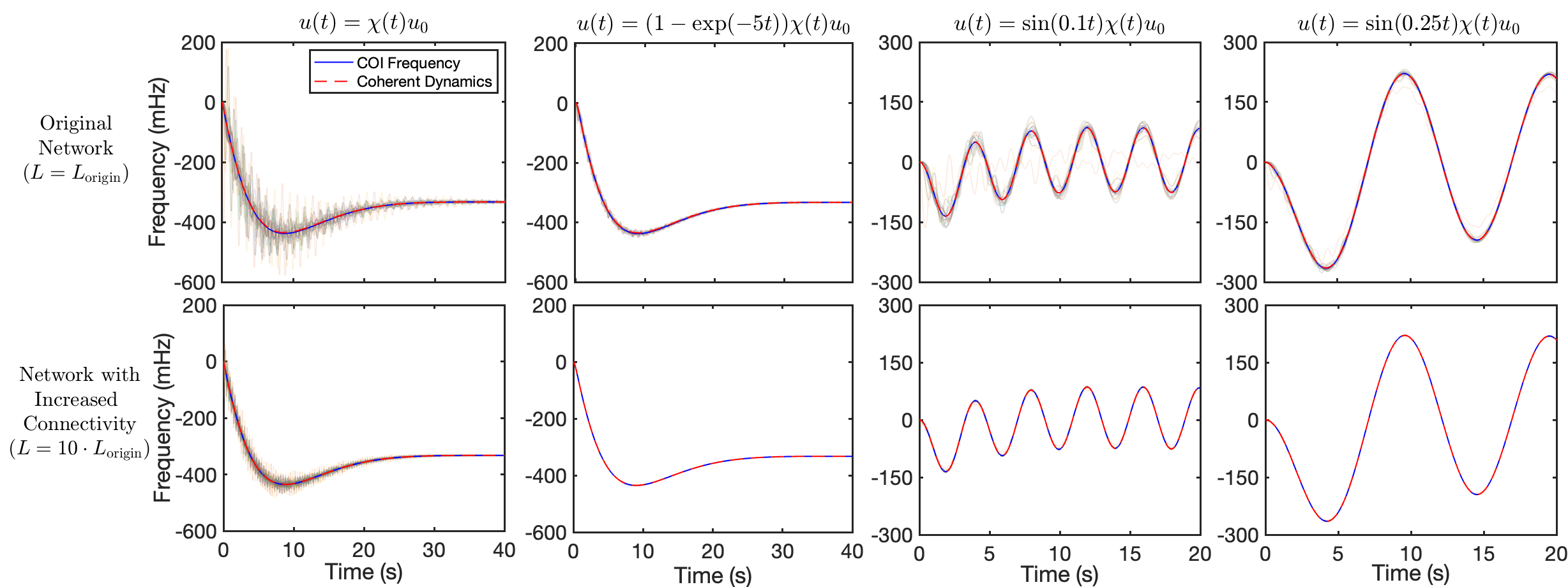
Figure 3: Coherent response of Icelandic Grid. Each column corresponds to a different input signal (from left to right: step, exponential approach, high-frequency sinusoidal, and low-frequency sinusoidal signal); The input signal has a shape $u_{0}=-e_{2}$, i.e., only the second node is subject to disturbance. Top row shows the responses of original icelandic grid, and the bottom row shows the responses of network with increased connectivity. Red dashed line shows the response of $\bar{g}(s)$ subject to the averaged input $\bar{u}(t)=\mathbb{1}^{\top}u(t)/n$. Blue solid line shows the Center-of-Inertia frequency of the grid $y_{\mathrm{COI}}=(\sum_{i=1}^{n}m_{i}y_{i})/(\sum_{i=1}^{n}m_{i})$.

6.1 Numerical verification

We verify our theoretical results, Theorem 6 and Theorem 9, with numerical simulations on the Icelandic power grid [47] modeled as in Fig 2. We plot in Fig. 3 the frequency response of the power network model subject to various input disturbances. the network step response is more coherent, i.e. response of every single node (generator) is getting closer to the one of the coherent dynamics $\bar{g}(s)$, when the network connectivity is scaled up, as suggested by Theorem 6. In addition, the network responds more coherently when subject to lower-frequency signals (See the second and forth column in Fig 3), as suggested by Theorem 9. But most importantly, the coherent dynamics $\bar{g}(s)$ provides a good characterization of the coherent response. We also plot the Center-of-Inertia frequency of the grid $y_{\mathrm{COI}}=(\sum_{i=1}^{n}m_{i}y_{i})/(\sum_{i=1}^{n}m_{i})$, which is generally used for frequency response assessment, and we see that it is well approximated by the response of $\bar{g}(s)$.

6.2 Aggregate dynamics of generator networks

The numerical simulations above suggest that the coherent dynamics $\bar{g}(s)$ characterize well the overall frequency response of generators in a grid. This leads to a general methodology to analyze the aggregate dynamics of such networks. Let

$$g_{\mathrm{aggr}}(s):=\frac{1}{n}\bar{g}(s)=\left(\sum_{i=1}^{n}g_{i}^{-1}(s)\right)\,.$$

Our analysis suggests that the transfer function $T(s)$ representing a network of generators is close $g_{\mathrm{aggr}}(s)\mathbb{1}\mathbb{1}^{\top}$ within the low-frequency range, for sufficiently high network connectivity $\lambda_{2}(L)$. We can also view $g_{\mathrm{aggr}}(s)$ as the aggregate generator dynamics, in the sense that it takes the sum of disturbances $\mathbb{1}^{\top}u=\sum_{i=1}^{n}u_{i}$ as its input, and its output represents the coherent response of all generators.

Such a notion of aggregate dynamics is important in modeling large-scale power networks[14]. Generally speaking, one seeks to find an aggregate dynamic model for a group of generators using the same structure (transfer function) as individual generator dynamics, i.e. when generator dynamics are modeled as $g_{i}(s)=g(s;\theta_{i})$, where $\theta_{i}$ is a vector of parameters representing physical properties of each generator, existing works [28, 35] propose methods to find aggregate dynamics of the form $g(s;\theta_{\mathrm{aggr}})$ for certain structures of $g(s;\theta)$. Our $g_{\mathrm{aggr}}(s)$ justifies their choices of $\theta_{\mathrm{aggr}}$, as shown in the following example.

Example 16.

For generators given by the swing model $g_{i}(s)=\frac{1}{m_{i}s+d_{i}}\,,$ where $m_{i},d_{i}$ are the inertia and damping of generator $i$, respectively. The aggregate dynamics are

$$g_{\mathrm{aggr}}(s)=\frac{1}{m_{\mathrm{aggr}}s+d_{\mathrm{aggr}}}\,,$$ (14)

where $m_{\mathrm{aggr}}=\sum_{i=1}^{n}m_{i}$ and $d_{\mathrm{aggr}}=\sum_{i=1}^{n}d_{i}$.

Here the parameters are $\theta=\{m,d\}$. The aggregate model given by (14) is consistent with the existing approach of choosing inertia $m$ and damping $d$ as the respective sums over all the coherent generators.

However, as we show in the next example, when one considers more involved models, it is challenging to find parameters that accurately fit the aggregate dynamics.

Example 17.

For generators given by the swing model with turbine droop $g_{i}(s)=\frac{1}{m_{i}s+d_{i}+\frac{r_{i}^{-1}}{\tau_{i}s+1}}\,,$ where $r_{i}^{-1}$ and $\tau_{i}$ are the droop coefficient and turbine time constant of generator $i$, respectively. The aggregate dynamics are given by

$$g_{\mathrm{aggr}}(s)=\frac{1}{m_{\mathrm{aggr}}s+d_{\mathrm{aggr}}+\sum_{i=1}^{n}\frac{r_{i}^{-1}}{\tau_{i}s+1}}\,.$$ (15)

Here the parameters are $\theta=\{m,d,r^{-1},\tau\}$. This example illustrates, in particular, the difficulty in aggregating generators with heterogeneous turbine time constants. If the $\tau_{i}$ are heterogeneous, then $g_{\mathrm{aggr}}(s)$ is a high-order transfer function and cannot be accurately represented by a single generator model parametrized by $\theta$. The aggregation of generators essentially asks for a low-order approximation of $g_{\mathrm{aggr}}(s)$. Our analysis reveals the fundamental limitation of using conventional approaches seeking aggregate dynamics with the same structure of individual generators. Furthermore, by characterizing the aggregate dynamics in the explicit form $g_{\mathrm{aggr}}(s)$, one can develop more accurate low-order approximation [48]. Lastly, we emphasize that our analysis does not depend on a specific model of generator dynamics $g_{i}(s)$, hence it provides a general methodology to aggregate coherent generator networks.

7 Conclusions

In this paper, we studies network coherence as a low-rank property of the transfer matrix $T(s)$ in the frequency domain. The analysis leads to useful characterizations of coordinated behavior and justifies the relation between network coherence and network effective algebraic connectivity. Our results suggest that network coherence is a frequency-dependent phenomenon, which is numerically illustrated in generator networks. Lastly, concentration results for large-scale networks are presented, revealing the exclusive role of the statistical distribution of node dynamics in determining the coherent dynamics of such networks. One interesting future work is to study the dynamic behavior of large-scale networks with multiple coherent groups. One could model the inter-community interactions by replacing the dynamics of each community with its coherent one, or more generally, a reduced one. Although clustering, i.e. finding communities, for homogeneous networks can be efficiently done by various graph-based methods, it is still open for research to find multiple coherent groups in heterogeneous dynamical networks.

Appendix A Proof of Lemma 1

Let $H=V^{\top}\mathrm{diag}\{g_{i}^{-1}(s_{0})\}V+f(s_{0})\Lambda$, such that (2) becomes $T(s)=VH^{-1}V^{\top}$. Then it is easy to see that

$$\left\lVert T(s_{0})-\frac{1}{n}\bar{g}(s_{0})\mathbb{1}\mathbb{1}^{\top}\right\rVert =\;\|T(s_{0})-\bar{g}(s_{0})Ve_{1}e_{1}^{\top}V^{\top}\|$$

$$=\;\left\lVert V\left(H^{-1}-\bar{g}(s_{0})e_{1}e_{1}^{\top}\right)V^{\top}\right\rVert$$

$$=\;\left\lVert H^{-1}-\bar{g}(s_{0})e_{1}e_{1}^{\top}\right\rVert\,,$$ (16)

where $e_{1}$ is the first column of identity matrix $I_{n}$. The first equality holds by noticing that $\frac{\mathbb{1}}{\sqrt{n}}$ is the first column of $V$.

With $V=\begin{bmatrix}\frac{\mathbb{1}}{\sqrt{n}}&V_{\perp}\end{bmatrix}$, we write $H$ in block matrix form:

$$H =\begin{bmatrix}\frac{\mathbb{1}^{\top}}{\sqrt{n}}\\ V_{\perp}^{\top}\end{bmatrix}\mathrm{diag}\{g_{i}^{-1}(s_{0})\}\begin{bmatrix}\frac{\mathbb{1}}{\sqrt{n}}&V_{\perp}\end{bmatrix}+f(s_{0})\Lambda$$

$$:=\begin{bmatrix}\bar{g}^{-1}(s_{0})&h^{\top}_{21}\\ h_{21}&H_{22}\end{bmatrix}\,,$$

where

$$\;h_{21}=V_{\perp}^{\top}\mathrm{diag}\{g_{i}^{-1}(s_{0})\}\frac{\mathbb{1}}{\sqrt{n}}\,,$$

$$\;H_{22}=V_{\perp}^{\top}\mathrm{diag}\{g_{i}^{-1}(s_{0})\}V_{\perp}+f(s_{0})\tilde{\Lambda}\,,$$

$$\;\tilde{\Lambda}=\mathrm{diag}\{\lambda_{2}(L),\cdots,\lambda_{n}(L)\}\,.$$

Inverting $H$ in its block form, we have

$$H^{-1}=\begin{bmatrix}a&-ah_{21}^{\top}H_{22}^{-1}\\ -aH_{22}^{-1}h_{21}&H_{22}^{-1}+aH_{22}^{-1}h_{21}h_{21}^{\top}H_{22}^{-1}\end{bmatrix}\,,$$

where $a=\frac{1}{\bar{g}^{-1}(s_{0})-h_{21}^{\top}H_{22}^{-1}h_{21}}$.

By our assumption, we have $\|\mathrm{diag}\{g_{i}^{-1}(s_{0})\}\|=\max_{1\leq i\leq n}|g_{i}^{-1}(s_{0})|\leq M_{2}\,,$ then

$$\|h_{21}\| =\;\left\lVert V_{\perp}^{\top}\mathrm{diag}\{g_{i}^{-1}(s_{0})\}\frac{\mathbb{1}}{\sqrt{n}}\right\rVert$$

$$\leq\;\|V_{\perp}\|\|\mathrm{diag}\{g_{i}^{-1}(s_{0})\}\|\frac{\|\mathbb{1}\|}{\sqrt{n}}\leq M_{2}\,,$$ (17)

and

$$\|H_{22}^{-1}\| =\;\|(f(s_{0})\tilde{\Lambda}+V_{\perp}^{\top}\mathrm{diag}\{g_{i}^{-1}(s_{0})\}V_{\perp})^{-1}\|$$

$$=\;\sigma_{\min}\left(f(s_{0})\tilde{\Lambda}+V_{\perp}^{\top}\mathrm{diag}\{g_{i}^{-1}(s_{0})\}V_{\perp}\right)$$

$$\leq\;\frac{1}{\sigma_{\min}(f(s_{0})\tilde{\Lambda})-\|V_{\perp}^{\top}\mathrm{diag}\{g_{i}^{-1}(s_{0})\}V_{\perp}\|}$$

$$\leq\;\frac{1}{\sigma_{\min}(f(s_{0})\tilde{\Lambda})-M_{2}}\leq\frac{1}{|f(s_{0})|\lambda_{2}(L)-M_{2}}\,,$$ (18)

whenever $|f(s_{0})|\lambda_{2}(L)>M_{2}$.

Lastly, when $|f(s_{0})|\lambda_{2}(L)>M_{2}+M_{2}^{2}M_{1}$, a similar reasoning as above, using (17) (18), and our assumption $|\bar{g}(s_{0})|\leq M_{1}$, gives

$$|a| \leq\;\frac{1}{|\bar{g}^{-1}(s_{0})|-\|h_{21}\|^{2}\|H_{22}^{-1}\|}$$

$$=\;\frac{(|f(s_{0})|\lambda_{2}(L)-M_{2})M_{1}}{|f(s_{0})|\lambda_{2}(L)-M_{2}-M_{1}M_{2}^{2}}\,.$$ (19)

Now we bound the norm of $H^{-1}-\bar{g}(s_{0})e_{1}e_{1}^{\top}$ by the sum of norms of all its blocks:

$$\;\|H^{-1}-\bar{g}(s_{0})e_{1}e_{1}^{\top}\|$$

$$\leq \;|a\bar{g}(s_{0})h_{21}^{\top}H_{22}^{-1}h_{21}|+2\|aH_{22}^{-1}h_{21}\|$$

$$\;\quad\qquad+\|H_{22}^{-1}+aH_{22}^{-1}h_{21}h_{21}^{\top}H_{22}^{-1}\|$$

$$\leq \;|a|\|H_{22}^{-1}\|(|\bar{g}(s_{0})|\|h_{21}\|^{2}+2\|h_{21}\|+\|h_{21}\|^{2}\|H_{22}^{-1}\|)$$

$$\;\quad\quad+\|H_{22}^{-1}\|\,,$$ (20)

Using (17)(18)(19), we can further upper bound (20) as

$$\|H^{-1}-\bar{g}(s_{0})e_{1}e_{1}^{\top}\|\leq\frac{\left(M_{1}M_{2}+1\right)^{2}}{|f(s_{0})|\lambda_{2}(L)-M_{2}-M_{1}M_{2}^{2}}\,.$$ (21)

This bound holds as long as $|f(s_{0})|\lambda_{2}(L)>M_{2}+M_{2}^{2}M_{1}$. Combining (16) and (21) gives the desired inequality.

Appendix B Proof of Theorem 6 and 9

When the input to the network is $U(s)$, the output response of the $i$-th node is

$$Y_{i}(s)=e_{i}^{\top}T(s)U(s)\,,$$

where $e_{i}$ is the $i$-th column of the identity matrix $I_{n}$.

Using Mellin’s inverse formula [38, Theorem 3.20], we have

$$\;|y_{i}(t)-\bar{y}(t)|$$

$$= \;\left|\frac{1}{2\pi j}\lim_{\omega\rightarrow\infty}\int_{\sigma-j\omega}^{\sigma+j\omega}e^{st}\left(Y_{i}(s)-e_{i}^{\top}\bar{g}(s)\mathbb{1}\frac{\mathbb{1}^{\top}}{n}U(s)\right)ds\right|$$

$$\leq \;\frac{e^{\sigma}}{2\pi}\lim_{\omega\rightarrow\infty}\int_{\sigma-j\omega}^{\sigma+j\omega}\left|e_{i}^{\top}T(s)U(s)-e_{i}^{\top}\bar{g}(s)\mathbb{1}\frac{\mathbb{1}^{\top}}{n}U(s)\right|ds$$

$$\leq \;\frac{e^{\sigma}}{2\pi}\lim_{\omega\rightarrow\infty}\int_{\sigma-j\omega}^{\sigma+j\omega}\left\lVert T(s)-\frac{1}{n}\bar{g}(s)\mathbb{1}\mathbb{1}^{\top}\right\rVert\|U(s)\|ds$$

$$= \;\frac{e^{\sigma}}{2\pi}\left((A)+(B)+(C)\right)\,,$$

where

$$(A)=\int_{\sigma-j\omega_{0}}^{\sigma+j\omega_{0}}\left\lVert T(s)-\frac{1}{n}\bar{g}(s)\mathbb{1}\mathbb{1}^{\top}\right\rVert\|U(s)\|ds\,,$$

$$(B)=\lim_{\omega\rightarrow\infty}\int_{\sigma+j\omega_{0}}^{\sigma+j\omega}\left\lVert T(s)-\frac{1}{n}\bar{g}(s)\mathbb{1}\mathbb{1}^{\top}\right\rVert\|U(s)\|ds\,,$$

$$(C)=\lim_{\omega\rightarrow\infty}\int_{\sigma-j\omega}^{\sigma-j\omega_{0}}\left\lVert T(s)-\frac{1}{n}\bar{g}(s)\mathbb{1}\mathbb{1}^{\top}\right\rVert\|U(s)\|ds\,.$$

Both proofs uses such decomposition. By our assumption,

$$(B) =\;\lim_{\omega\rightarrow\infty}\int_{\sigma+j\omega_{0}}^{\sigma+j\omega}\left\lVert T(s)-\frac{1}{n}\bar{g}(s)\mathbb{1}\mathbb{1}^{\top}\right\rVert\|U(s)\|ds$$

$$\leq\;\lim_{\omega\rightarrow\infty}\int_{\sigma+j\omega_{0}}^{\sigma+j\omega}\left(\left\lVert T(s)\right\rVert+\left\lVert\bar{g}(s)\right\rVert\right)\|U(s)\|ds$$

$$\leq\;2\gamma\lim_{\omega\rightarrow\infty}\int_{\sigma+j\omega_{0}}^{\sigma+j\omega}\|U(s)\|ds\,,$$

where the last inequality uses the fact that $\bar{g}(s)$ and $T(s)$ are stable: $\|\bar{g}(s)\|_{\mathcal{H}_{\infty}},\|T(s)\|_{\mathcal{H}_{\infty}}\leq\gamma$. Because for the real input signals, we have $U(s^{*})=U^{*}(s)$, hence $\int^{\sigma-j\omega_{0}}_{\sigma-j\omega}\|U(s)\|ds=\int^{\sigma+j\omega}_{\sigma+j\omega_{0}}\|U(s)\|ds\,,$ which leads to

$$(C)\leq 2\gamma\lim_{\omega\rightarrow\infty}\int_{\sigma+j\omega_{0}}^{\sigma+j\omega}\|U(s)\|ds\,.$$

Now we are ready to prove Theorem 6 and 9. [Proof of Theorem 6] First of all, Mellin’s inverse formula requires that the vertical line $Re(s)=\sigma$ is on the right of all poles of the signal. This is the case from our assumption that $\sup_{Re(s)>\sigma}\|U(s)\|<+\infty$ and that $T(s),\bar{g}(s)$ being stable.

By the assumption that $\lim_{\omega\rightarrow\infty}\int_{\sigma+j0}^{\sigma+j\omega}\|U(s)\|ds$ is finite, one can pick an $\omega_{0}>0$, such that

$$\lim_{\omega\rightarrow\infty}\int_{\sigma+j\omega_{0}}^{\sigma+j\omega}\|U(s)\|ds\leq\frac{2\pi\epsilon}{6e^{\sigma}\gamma}\,,$$

which leads to

$$(B) \leq\;2\gamma\lim_{\omega\rightarrow\infty}\int_{\sigma+j\omega_{0}}^{\sigma+j\omega}\|U(s)\|ds\leq\frac{2\pi\epsilon}{3e^{\sigma}}\,.$$

Similarly, we have $(C)\leq\frac{2\pi\epsilon}{3e^{\sigma}}$.

For the remaining term, we have

$$(A) =\;\int_{\sigma-j\omega_{0}}^{\sigma+j\omega_{0}}\left\lVert T(s)-\frac{1}{n}\bar{g}(s)\mathbb{1}\mathbb{1}^{\top}\right\rVert\|U(s)\|ds$$

$$\leq\;\sup_{w\in[-w_{0},w_{0}]}\left\lVert T(\sigma+jw)-\frac{1}{n}\bar{g}(\sigma+jw)\mathbb{1}\mathbb{1}^{\top}\right\rVert$$

$$\;\quad\quad\times\int_{\sigma-j\omega_{0}}^{\sigma+j\omega_{0}}\|U(s)\|ds$$

Since $[\sigma-j\omega_{0},\sigma+j\omega_{0}]$ is a compact set that satisfies the assumption in Theorem 2, we have

$$\lim_{\lambda_{2}(L)\rightarrow\infty}\sup_{w\in[-w_{0},w_{0}]}\left\lVert T(\sigma+jw)-\frac{1}{n}\bar{g}(\sigma+jw)\mathbb{1}\mathbb{1}^{\top}\right\rVert=0\,.$$

Therefore, for sufficiently large $\lambda_{2}(L)$, we have $(A)\leq\frac{2\pi\epsilon}{3e^{\sigma}}$. Combining the upperbounds for $(A),(B),(C)$, we have

$$|y_{i}(t)-\bar{y}(t)|\leq\epsilon\,.$$

Notice that the choice of $\lambda_{2}(L)$ does not depends on time $t$, hence this inequality holds for all $t>0$.

[Proof of Theorem 9] Here, the input is a sinusoidal signal $U(s)=\frac{\alpha}{s^{2}+\alpha^{2}}u_{0},u_{0}\in\mathbb{S}^{n-1}$. Mellin’s inverse formula requires that the vertical line $Re(s)=\sigma$ is on the right of all poles of the signal, which is satisfied under any choice $\sigma>0$. For our purpose, we pick

$$\sigma=\alpha,\omega_{0}=K\alpha\,,$$

for some $K>0$ (to be determined later). By our assumption,

$$(B) \leq\;2\gamma\lim_{\omega\rightarrow\infty}\int_{\sigma+j\omega_{0}}^{\sigma+j\omega}\left|\frac{\alpha}{s^{2}+\alpha^{2}}\right|\|u_{0}\|ds$$

$$=\;2\gamma\int_{\omega_{0}}^{+\infty}\frac{\alpha}{|(\sigma+j\omega)^{2}+\alpha^{2}|}d\omega$$

$$=\;2\gamma\int_{K\alpha}^{+\infty}\frac{\alpha}{|(\alpha+j\omega)^{2}+\alpha^{2}|}d\omega$$

$$=\;2\gamma\int_{K\alpha}^{+\infty}\frac{\alpha}{\sqrt{4\alpha^{4}+\omega^{4}}}d\omega$$

$$\leq\;2\sqrt{2}\gamma\int_{K\alpha}^{+\infty}\frac{\alpha}{2\alpha^{2}+\omega^{2}}d\omega$$

$$=\;\gamma\left(\pi-2\arctan\left(\frac{K}{\sqrt{2}}\right)\right)\,,$$ (22)

where the last inequality use the fact that for $a,b>0$, we have

$$\sqrt{a^{2}+b^{2}}\geq(a+b)/\sqrt{2}\,.$$

Similarly, we have

$$(C)\leq\gamma\left(\pi-2\arctan\left(\frac{K}{\sqrt{2}}\right)\right)\,.$$ (23)

For the remaining term, we use the result in the proof of Theorem 3: $\exists\delta>0$, such that $\forall s\in\mathcal{B}(0,\delta)$ such that

$$\left\lVert T(s)-\frac{1}{n}\bar{g}(s)\mathbb{1}\mathbb{1}^{\top}\right\rVert\leq\frac{2\left(M_{1}M_{2}+1\right)^{2}}{|f(s)|\lambda_{2}(L)}\,,$$

for some $M_{1},M_{2}>0$. Then as long as we pick $\alpha,K$ appropriately such that $|\sigma+j\omega_{0}|\leq\delta$, i.e., $\sqrt{1+K^{2}}\alpha\leq\delta$, we have

$$(A) =\;\int_{\sigma-j\omega_{0}}^{\sigma+j\omega_{0}}\left\lVert T(s)-\frac{1}{n}\bar{g}(s)\mathbb{1}\mathbb{1}^{\top}\right\rVert\left|\frac{\alpha}{s^{2}+\alpha^{2}}\right|ds$$

$$\leq\;\int_{\sigma-j\omega_{0}}^{\sigma+j\omega_{0}}\frac{2\left(M_{1}M_{2}+1\right)^{2}}{|f(s)|\lambda_{2}(L)}\left|\frac{\alpha}{s^{2}+\alpha^{2}}\right|ds$$

$$=\;\int_{\sigma-j\omega_{0}}^{\sigma+j\omega_{0}}\frac{2\left(M_{1}M_{2}+1\right)^{2}}{\lambda_{2}(L)/|s|}\frac{\alpha}{|s^{2}+\alpha^{2}|}ds$$

$$=\frac{2\left(M_{1}M_{2}+1\right)^{2}}{\lambda_{2}(L)}\;\int_{\sigma-j\omega_{0}}^{\sigma+j\omega_{0}}\frac{|s|\alpha}{|s^{2}+\alpha^{2}|}ds$$

$$=\frac{4\left(M_{1}M_{2}+1\right)^{2}}{\lambda_{2}(L)}\;\int_{0}^{K\alpha}\frac{|\alpha+j\omega|\alpha}{|(\alpha+j\omega)^{2}+\alpha^{2}|}d\omega$$

$$=\frac{4\left(M_{1}M_{2}+1\right)^{2}}{\lambda_{2}(L)}\;\int_{0}^{K\alpha}\frac{\sqrt{\alpha^{2}+\omega^{2}}\alpha}{\sqrt{4\alpha^{4}+\omega^{4}}}d\omega$$

$$\leq\;\frac{2\sqrt{2}\left(M_{1}M_{2}+1\right)^{2}}{\lambda_{2}(L)}\;\int_{0}^{K\alpha}\frac{2(\alpha+\omega)\alpha}{2\alpha^{2}+\omega^{2}}d\omega\,,$$

where the last equality used the fact that for $a,b>0$, we have

$$a+b\geq\sqrt{a^{2}+b^{2}}\geq(a+b)/\sqrt{2}\,,$$

to upper and lower bound the numerator and denominator respectively. Notice that

$$\;\int_{0}^{K\alpha}\frac{2(\alpha+\omega)\alpha}{2\alpha^{2}+\omega^{2}}d\omega$$

$$=\;\alpha\left(\sqrt{2}\arctan\left(\frac{K}{\sqrt{2}}\right)+\log\left(1+\frac{K^{2}}{2}\right)\right)$$

$$\leq\;2\alpha\log\left(\frac{K^{2}}{2}\right)\,,$$ (24)

for sufficiently large $K$. We have

$$(A)\leq\frac{4\sqrt{2}\left(M_{1}M_{2}+1\right)^{2}}{\lambda_{2}(L)}\alpha\log\left(\frac{K^{2}}{2}\right)\,.$$ (25)

The last step is to find the right choice of $\alpha,K$. Given $\epsilon>0$, pick a $K>0$, such that

$$2\gamma\left(\pi-2\arctan\left(\frac{K}{\sqrt{2}}\right)\right)\leq\frac{\epsilon\pi}{2}\,.$$

Generally such a $K$ is sufficient for (24) to hold. With this choice of $K$, let

$$\;\alpha_{0}:=$$

$$\;\min\left\{\log 2,\frac{\epsilon\pi\lambda_{2}(L)}{8\sqrt{2}(M_{1}M_{2}+1)^{2}\log\left(\frac{K^{2}}{2}\right)},\frac{\delta}{\sqrt{1+K^{2}}}\right\}\,.$$

Then, $\forall\alpha\leq\alpha_{0}$, combining (22)(23)(25), we have

$$\;|y_{i}(t)-\bar{y}(t)|$$

$$\;\leq\frac{e^{\sigma}}{2\pi}((A)+(B)+(C))$$

$$\;\leq\frac{e^{\alpha_{0}}}{2\pi}\left(2\gamma\left(\pi-2\arctan\left(\frac{K}{\sqrt{2}}\right)\right)\right.+$$

$$\;\qquad\left.\frac{4\sqrt{2}\left(M_{1}M_{2}+1\right)^{2}}{\lambda_{2}(L)}\alpha\log\left(\frac{K^{2}}{2}\right)\right)$$

$$\leq\;\frac{1}{\pi}\left(\frac{\epsilon\pi}{2}+\frac{\epsilon\pi}{2}\right)=\epsilon\,.$$

Notice that the choice of $\alpha_{0},K$ does not depends on time $t$, nor the node index $i$, hence this inequality holds for all $t>0$ and all $i\in[n]$.

Appendix C Proof of Theorem 7

For each $g_{i}(s),i=1,\cdots,n$, we have, by the OSP property,

$$Re(g_{i}(s))\geq\epsilon|g_{i}(s)|^{2},\forall Re(s)>0\,.$$

That is,

$$Re(G(s))\succeq\epsilon G^{*}(s)G(s)\,,$$

or equivalently, $\begin{bmatrix}G(s)\\ I\end{bmatrix}^{*}\begin{bmatrix}-\epsilon I&I\\ I&0\end{bmatrix}\begin{bmatrix}G(s)\\ I\end{bmatrix}\succeq 0\,.$ Since $g_{i}(s)$ are all OSP, then $g_{i}(s)$ is positive real [49]. A positive real function that is not zero function has no zero nor pole on the left half plane. Therefore $g_{i}(s)$ are invertible for all $Re(s)>0$, which ensures that $G(s)$ is invertible for all $Re(s)>0$. Then

$$(G^{*}(s))^{-1}\begin{bmatrix}G(s)\\ I\end{bmatrix}^{*}\begin{bmatrix}-\epsilon I&I\\ I&0\end{bmatrix}\begin{bmatrix}G(s)\\ I\end{bmatrix}G^{-1}(s)\succeq 0\,,$$

which is

$$\begin{bmatrix}I\\ G^{-1}(s)\end{bmatrix}^{*}\begin{bmatrix}-\epsilon I&I\\ I&0\end{bmatrix}\begin{bmatrix}I\\ G^{-1}(s)\end{bmatrix}\succeq 0\,.$$ (26)

Notice that

$$T(s)=(I+G(s)f(s)L)^{-1}G(s)=(G^{-1}(s)+f(s)L)^{-1}\,,$$

then from (26) and the fact that $f(s)$ is PR, we have

$$\;\begin{bmatrix}I\\ T^{-1}(s)\end{bmatrix}^{*}\begin{bmatrix}-\epsilon I&I\\ I&0\end{bmatrix}\begin{bmatrix}I\\ T^{-1}(s)\end{bmatrix}$$

$$= \;\begin{bmatrix}I\\ G^{-1}(s)+f(s)L\end{bmatrix}^{*}\begin{bmatrix}-\epsilon I&I\\ I&0\end{bmatrix}\begin{bmatrix}I\\ G^{-1}(s)+f(s)L\end{bmatrix}$$

$$= \;\begin{bmatrix}I\\ G^{-1}(s)\end{bmatrix}^{*}\begin{bmatrix}-\epsilon I&I\\ I&0\end{bmatrix}\begin{bmatrix}I\\ G^{-1}(s)\end{bmatrix}+[f^{*}(s)+f(s)]L$$

$$\succeq \;\begin{bmatrix}I\\ G^{-1}(s)\end{bmatrix}^{*}\begin{bmatrix}-\epsilon I&I\\ I&0\end{bmatrix}\begin{bmatrix}I\\ G^{-1}(s)\end{bmatrix}\succeq 0\,.$$

Now for sufficiently large $\gamma>0$, we have

$$\begin{bmatrix}-\epsilon I&I\\ I&0\end{bmatrix}+\begin{bmatrix}\frac{\epsilon}{2}I&0\\ 0&-\gamma^{2}\frac{\epsilon}{2}I\end{bmatrix}=\begin{bmatrix}-\frac{\epsilon}{2}I&I\\ I&-\gamma^{2}\frac{\epsilon}{2}I\end{bmatrix}\preceq 0\,,$$

since its Schur complement $(-\frac{\epsilon}{2}+\frac{2}{\epsilon\gamma^{2}})I\preceq 0$ for large $\gamma$. Therefore,

$$\;\begin{bmatrix}I\\ T^{-1}(s)\end{bmatrix}^{*}\begin{bmatrix}-\frac{\epsilon}{2}I&0\\ 0&\gamma^{2}\frac{\epsilon}{2}I\end{bmatrix}\begin{bmatrix}I\\ T^{-1}(s)\end{bmatrix}$$

$$\succeq \;\begin{bmatrix}I\\ T^{-1}(s)\end{bmatrix}^{*}\begin{bmatrix}-\epsilon I&I\\ I&0\end{bmatrix}\begin{bmatrix}I\\ T^{-1}(s)\end{bmatrix}\succeq 0\,,$$

which is exactly, $\gamma^{2}\frac{\epsilon}{2}(T^{-1}(s))^{*}(T^{-1}(s))\succeq\frac{\epsilon}{2}I\,.$ This shows that

$$\sigma_{min}^{2}(T^{-1}(s))\geq\frac{1}{\gamma^{2}},\forall Re(s)>0\,,$$ (27)

which is equivalent to $\|T(s)\|_{2}\leq\gamma\,,\forall Re(s)>0\,.$ Moreover, (27) implies

$$|\bar{g}^{-1}(s)|=\left|\frac{\mathbb{1}^{\top}}{\sqrt{n}}T^{-1}(s)\frac{\mathbb{1}}{\sqrt{n}}\right|^{2}\geq\frac{1}{\gamma^{2}},\forall Re(s)>0\,,$$

which is equivalent to $\|\bar{g}(s)\|_{2}\leq\gamma,\forall Re(s)>0$.

References

- [1] H. Min and E. Mallada, “Dynamics concentration of large-scale tightly-connected networks,” in IEEE 58th Conf. on Decision and Control, pp. 758–763, 2019.
- [2] P. C. Bressloff and S. Coombes, “Travelling waves in chains of pulse-coupled integrate-and-fire oscillators with distributed delays,” Physica D: Nonlinear Phenomena, vol. 130, no. 3-4, pp. 232–254, 1999.
- [3] I. Z. Kiss, Y. Zhai, and J. L. Hudson, “Emerging coherence in a population of chemical oscillators,” Science, vol. 296, no. 5573, pp. 1676–1678, 2002.
- [4] M. H. DeGroot, “Reaching a consensus,” Journal of the American Statistical Association, vol. 69, no. 345, pp. 118–121, 1974.
- [5] R. E. Mirollo and S. H. Strogatz, “Synchronization of pulse-coupled biological oscillators,” SIAM Journal on Applied Mathematics, vol. 50, no. 6, pp. 1645–1662, 1990.
- [6] Y. Jiang, R. Pates, and E. Mallada, “Performance tradeoffs of dynamically controlled grid-connected inverters in low inertia power systems,” in 56th IEEE Conf. on Decision and Control, pp. 5098–5105, 12 2017.
- [7] F. Paganini and E. Mallada, “Global analysis of synchronization performance for power systems: Bridging the theory-practice gap,” IEEE Trans. Automat. Contr., vol. 65, no. 7, pp. 3007–3022, 2020.
- [8] E. Mallada, X. Meng, M. Hack, L. Zhang, and A. Tang, “Skewless network clock synchronization without discontinuity: Convergence and performance,” IEEE/ACM Transactions on Networking (TON), vol. 23, pp. 1619–1633, 10 2015.
- [9] E. Mallada, Distributed synchronization in engineering networks: The Internet and electric power girds. PhD thesis, Electrical and Computer Engineering, Cornell University, 01 2014.
- [10] R. Sepulchre, D. Paley, and N. Leonard, “Stabilization of planar collective motion with limited communication,” IEEE Trans. Automat. Contr., vol. 53, no. 3, pp. 706–719, 2008.
- [11] R. Olfati-Saber, J. A. Fax, and R. M. Murray, “Consensus and cooperation in networked multi-agent systems,” Proceedings of the IEEE, vol. 95, no. 1, pp. 215–233, 2007.
- [12] A. Jadbabaie, J. Lin, and A. Morse, “Coordination of groups of mobile autonomous agents using nearest neighbor rules,” IEEE Trans. Automat. Contr., vol. 48, no. 6, pp. 988–1001, 2003.
- [13] B. Bamieh, M. R. Jovanovic, P. Mitra, and S. Patterson, “Coherence in large-scale networks: Dimension-dependent limitations of local feedback,” IEEE Trans. Automat. Contr., vol. 57, no. 9, pp. 2235–2249, 2012.
- [14] J. H. Chow, Power system coherency and model reduction. New York, NY, USA: Springer, 2013.
- [15] J. H. Chow, Time-scale modeling of dynamic networks with applications to power systems. Springer, 1982.
- [16] G. N. Ramaswamy, L. Rouco, O. Fillatre, G. C. Verghese, P. Panciatici, B. C. Lesieutre, and D. Peltier, “Synchronic modal equivalencing (sme) for structure-preserving dynamic equivalents,” IEEE Transactions on Power Systems, vol. 11, no. 1, pp. 19–29, 1996.
- [17] D. Romeres, F. Dörfler, and F. Bullo, “Novel results on slow coherency in consensus and power networks,” in 2013 European Control Conference (ECC), pp. 742–747, 2013.
- [18] I. Tyuryukanov, M. Popov, M. A. M. M. van der Meijden, and V. Terzija, “Slow coherency identification and power system dynamic model reduction by using orthogonal structure of electromechanical eigenvectors,” IEEE Transactions on Power Systems, vol. 36, no. 2, pp. 1482–1492, 2021.
- [19] J. Fritzsch and P. Jacquod, “Long wavelength coherency in well connected electric power networks,” IEEE Access, vol. 10, pp. 19986–19996, 2022.
- [20] Y. Jiang, R. Pates, and E. Mallada, “Dynamic droop control in low inertia power systems,” IEEE Transactions on Automatic Control, vol. 66, pp. 3518–3533, 8 2021.
- [21] Y. Jiang, A. Bernstein, P. Vorobev, and E. Mallada, “Grid-forming frequency shaping control in low inertia power systems,” IEEE Control Systems Letters (L-CSS), vol. 5, pp. 1988–1993, 12 2021. also in ACC 2021.
- [22] E. Ekomwenrenren, Z. Tang, J. W. Simpson-Porco, E. Farantatos, M. Patel, and H. Hooshyar, “Hierarchical coordinated fast frequency control using inverter-based resources,” IEEE Transactions on Power Systems, vol. 36, no. 6, pp. 4992–5005, 2021.
- [23] E. Tegling, B. Bamieh, and H. Sandberg, “Localized high-order consensus destabilizes large-scale networks,” in 2019 American Control Conference (ACC), pp. 760–765, July 2019.
- [24] H. G. Oral, E. Mallada, and D. F. Gayme, “Performance of first and second order linear networked systems over digraphs,” in IEEE 56th Annu. Conf. on Decision and Control, pp. 1688–1694, Dec 2017.
- [25] B. Bamieh and D. F. Gayme, “The price of synchrony: Resistive losses due to phase synchronization in power networks,” in 2013 American Control Conference, pp. 5815–5820, 2013.
- [26] M. Andreasson, E. Tegling, H. Sandberg, and K. H. Johansson, “Coherence in synchronizing power networks with distributed integral control,” in IEEE 56th Annu. Conf. on Decision and Control, pp. 6327–6333, Dec 2017.
- [27] M. Pirani, J. W. Simpson-Porco, and B. Fidan, “System-theoretic performance metrics for low-inertia stability of power networks,” in 2017 IEEE 56th Annual Conference on Decision and Control (CDC), pp. 5106–5111, 2017.
- [28] A. J. Germond and R. Podmore, “Dynamic aggregation of generating unit models,” IEEE Trans. Power App. Syst., vol. PAS-97, pp. 1060–1069, July 1978.
- [29] R. Olfati-Saber and R. Murray, “Consensus problems in networks of agents with switching topology and time-delays,” IEEE Trans. Automat. Contr., vol. 49, no. 9, pp. 1520–1533, 2004.
- [30] Y. Ghaedsharaf, M. Siami, C. Somarakis, and N. Motee, “Centrality in time-delay consensus networks with structured uncertainties,” arXiv preprint arXiv:1902.08514, 2019.
- [31] S. Nair and N. Leonard, “Stable synchronization of mechanical system networks,” SIAM Journal on Control and Optimization, vol. 47, no. 2, pp. 661–683, 2008.
- [32] H. Kim, H. Shim, and J. Seo, “Output consensus of heterogeneous uncertain linear multi-agent systems,” IEEE Trans. Automat. Contr., vol. 56, no. 1, pp. 200–206, 2011.
- [33] P. Wieland, R. Sepulchre, and F. Allgöwer, “An internal model principle is necessary and sufficient for linear output synchronization,” Automatica, vol. 47, no. 5, pp. 1068–1074, 2011.
- [34] P. M. Anderson and M. Mirheydar, “A low-order system frequency response model,” IEEE Trans. Power Syst., vol. 5, no. 3, pp. 720–729, 1990.
- [35] S. S. Guggilam, C. Zhao, E. Dall’Anese, Y. C. Chen, and S. V. Dhople, “Optimizing DER participation in inertial and primary-frequency response,” IEEE Trans. Power Syst., vol. 33, pp. 5194–5205, Sep. 2018.
- [36] W. Rudin et al., Principles of mathematical analysis, vol. 3. McGraw-hill New York, 1964.
- [37] H. Min, R. Pates, and E. Mallada, “Coherence and concentration in tightly-connected networks,” arXiv preprint arXiv:2101.00981, 2021.
- [38] G. E. Dullerud and F. Paganini, A course in robust control theory: a convex approach, vol. 36. Springer Science & Business Media, 2013.
- [39] H. Marquez and C. Damaren, “Comments on ”strictly positive real transfer functions revisited,” IEEE Transactions on Automatic Control, vol. 40, no. 3, pp. 478–479, 1995.
- [40] I. Lestas and G. Vinnicombe, “Scalable decentralized robust stability certificates for networks of interconnected heterogeneous dynamical systems,” IEEE Transactions on Automatic Control, vol. 51, no. 10, pp. 1613–1625, 2006.
- [41] U. T. Jönsson and C.-Y. Kao, “A scalable robust stability criterion for systems with heterogeneous lti components,” IEEE Transactions on Automatic Control, vol. 55, no. 10, pp. 2219–2234, 2010.
- [42] R. Pates and E. Mallada, “Robust scale-free synthesis for frequency control in power systems,” IEEE Transactions on Control of Network Systems, vol. 6, no. 3, pp. 1174–1184, 2019.
- [43] G. Ramaswamy, G. Verghese, L. Rouco, C. Vialas, and C. DeMarco, “Synchrony, aggregation, and multi-area eigenanalysis,” IEEE Transactions on Power Systems, vol. 10, no. 4, pp. 1986–1993, 1995.
- [44] F. Wu and N. Narasimhamurthi, “Coherency identification for power system dynamic equivalents,” IEEE Transactions on Circuits and Systems, vol. 30, no. 3, pp. 140–147, 1983.
- [45] S. Sastry and P. Varaiya, “Coherency for interconnected power systems,” IEEE Transactions on Automatic Control, vol. 26, no. 1, pp. 218–226, 1981.
- [46] M. Z. Q. Chen and M. C. Smith, “A note on tests for positive-real functions,” IEEE Transactions on Automatic Control, vol. 54, no. 2, pp. 390–393, 2009.
- [47] U. of Edinburgh, “Power systems test case archive.” Mar. 2003.
- [48] H. Min, F. Paganini, and E. Mallada, “Accurate reduced-order models for heterogeneous coherent generators,” IEEE Contr. Syst. Lett., vol. 5, no. 5, pp. 1741–1746, 2021.
- [49] H. K. Khalil and J. W. Grizzle, Nonlinear systems, vol. 3. Prentice hall Upper Saddle River, NJ, 2002.