Recovery of steady rotational wave profiles from pressure measurements at the bed

Abstract.

We derive equations relating the pressure at a flat seabed and the free-surface profile for steady gravity waves with constant vorticity. The resulting set of nonlinear equations enables the recovery of the free surface from pressure measurements at the bed. Furthermore, the flow vorticity is determined solely from the bottom pressure as part of the recovery method. This approach is applicable even in the presence of stagnation points and its efficiency is illustrated via numerical examples.

1. Introduction

In this paper, we present a formulation of the rotational water wave problem which enables the recovery of nonlinear surface gravity wave profiles from pressure measurements at the seabed, for steady flows with constant vorticity. The determination of the wave profile is achieved by numerically solving a set of nonlinear equations, with our inverse recovery procedure having the significant side-benefit of also determining the vorticity $\omega$ directly from bottom pressure measurements. The presence of vorticity greatly complicates the mathematical problem, and the recovery of fully nonlinear rotational water wave profiles from pressure measurements has hitherto proven unattainable (although explicit surface-profile recovery formulae for linear, and weakly nonlinear, rotational water waves were derived by [18] for arbitrary vorticity distributions).

The reconstruction of water wave surface profiles from bottom pressure measurements is a theoretically challenging issue with important applications in marine engineering. Measuring the surface of water waves directly is difficult and costly, particularly in the ocean, so a commonly employed alternative is to calculate the free-surface profile of water waves using measurements from submerged pressure transducers. To do so requires the construction of either a suitable pressure-transfer function (for linear waves), or a surface reconstruction procedure (for nonlinear waves), the determination of which corresponds to a difficult mathematical problem.

Until quite recently, most surface reconstruction formulae were applicable only to the restricted setting of linear water waves, and even then solely for irrotational flows. First approaches towards surface reconstruction formulae for nonlinear irrotational waves appeared in [11, 21], however these formulae are quite involved. Exact tractable relations were derived in [3, 7] which permit a straightforward numerical procedure for deriving the free surface from the bottom pressure. A significant advantage of these approaches is that they work directly with nonlinear waves in the physical plane, allowing recovery of nonlinear wave-profiles up to, and including, Stokes wave of greatest height [9]. The robustness of this nonlinear wave surface reconstruction approach is further illustrated in this paper by expanding it to encompass flows with constant vorticity.

Incorporating vorticity in the water wave problem is vital for capturing fundamental physical processes relating to wave-current interactions [22], however it significantly complicates all theoretical considerations [10]. We note that while it was rigorously proven by [17] that the profile-recovery problem is well-posed for nonlinear solitary waves with arbitrary (real analytic) vorticity distributions, it remains an open question whether the inverse recovery problem is well-posed for periodic waves. Even in the simplified setting of constant vorticity, the water wave problem exhibits features not encountered in the irrotational case. In particular, we note such flows may contain stagnation points (and critical layers) in the fluid interior, and waves which possess overhanging profiles. The possibility of overhanging waves was first observed numerically [16, 20] and their possible existence was recently rigorously proven [15, 13]. We note that the surface recovery approach introduced in this paper is applicable to flows containing stagnation points, however we must exclude overhanging profiles a priori. It is assumed throughout that the surface profile is a graph (overhanging waves cannot occur for ‘downstream’ waves, c.f. [14]).

2. Preliminaries

In the frame of reference moving with a travelling wave of permanent shape, the flow beneath the wave reduces to a steady motion with respect to the moving coordinate system. Thus, the wave phase velocity $c$ is constant in any Galilean frame of reference. Let $(x,y)$ be a Cartesian coordinate system moving with the wave, $x$ being the horizontal coordinate and $y$ the upward vertical coordinate. We define accordingly the fluid domain as $\Omega=\{(x,y):x\in\mathds{R},-0pt\leqslant y\leqslant\eta(x)\}$, where $y=-0pt$ and $y=\eta(x)$ correspond, respectively, to the solid bottom and the free-surface (both impermeable). In addition, $\left(u(x,y),v(x,y)\right)$ denotes the velocity field in the moving frame. We assume the wave is $L=(2\pi/k$)-periodic (with $k\to 0$ for solitary waves) in the $x$-direction, and we denote by $y=0$ the mean water level. The latter equation expresses the fact that $\left<\eta\right>=0$, where $\left<\cdot\right>$ is the Eulerian average operator over one period, that is,

(1) $$\left<\eta\right>\stackrel{{\scriptstyle\text{\tiny{def}}}}{{=}}\frac{k}{2\pi}\int_{-\pi/k}^{\pi/k}\eta(x)\mathrm{d}x=0.$$

The flow is governed by the balance between the restoring gravity force and the inertia of the system. With constant density $\rho>0$, the equation of mass conservation and Euler equations (defined in $\Omega$) are, respectively,

$(2a,b,c)$ $$\partial_{x}u+\partial_{y}v=0,\quad u\/\partial_{x}u+v\/\partial_{y}u=-\partial_{x}P/\rho,\quad u\/\partial_{x}v+v\/\partial_{y}v=-\partial_{y}P/\rho-g,$$

where $P(x,y)$ denotes the pressure. As a general notation, subscripts ‘b’ denote all quantities written at the bed $y=-0pt$ whereas subscripts ‘s’ denote all quantities written at the free surface $y=\eta(x)$. The effect of surface tension being neglected, on the free surface we must have the dynamic boundary condition

(3) $${P}_{\mathrm{s}}=P_{\text{atm}},$$

where $P_{\text{atm}}$ is the (constant) atmospheric pressure. The free surface and the rigid bed are impermeable interfaces, giving the kinematic boundary conditions (with $\eta_{x}\stackrel{{\scriptstyle\text{\tiny{def}}}}{{=}}\mathrm{d}\eta(x)/\mathrm{d}x$)

$(4a,b)$ $${v}_{\mathrm{s}}={u}_{\mathrm{s}}\eta_{x},\qquad{v}_{\mathrm{b}}=0,$$

respectively, while the rotational character of the flow is ensured by requiring

(5) $$\partial_{x}v-\partial_{y}u\stackrel{{\scriptstyle\text{\tiny{def}}}}{{=}}\omega\quad(=\text{constant}).$$

Equations ($(2a,b,c)$)–(5) are the governing equations for rotational (of constant vorticity $\omega$) travelling water waves in a frame of reference moving with the wave.

For incompressible flows where ($(2a,b,c)$a) holds we can define a streamfunction $\psi$ such that $u=\partial_{y}\psi$ and $v=-\partial_{x}\psi$. As the flow is steady and the free-surface is impermeable, it follows that the free-surface is a streamline, that is, the streamfunction is constant $\psi={\psi}_{\mathrm{s}}$ at the free-surface (similarly, the streamfunction is constant $\psi={\psi}_{\mathrm{b}}$ at the bed).

Equations ($(2a,b,c)$) can be integrated to

(6) $$2p+2gy+u^{2}+v^{2}={B}_{\mathrm{s}}-2\omega(\psi-{\psi}_{\mathrm{s}}),$$

for some constant ${B}_{\mathrm{s}}$, where $p(x,y)\stackrel{{\scriptstyle\text{\tiny{def}}}}{{=}}[P(x,y)-P_{\text{atm}}]/\rho$ is a normalised relative pressure. Equation (6) is a Bernoulli equation, and we note that the Bernoulli integral $B(\psi)\stackrel{{\scriptstyle\text{\tiny{def}}}}{{=}}{B}_{\mathrm{s}}-2\omega(\psi-{\psi}_{\mathrm{s}})$ is constant for an irrotational motion (i.e., when $\omega=0$).

3. Definition of the parameters

From the definition (1) of the mean water level and by averaging expression (6) written at the free surface, we obtain a definition for the constant ${B}_{\mathrm{s}}$ in the form

(7) $${B}_{\mathrm{s}}=\left<{u}_{\mathrm{s}}^{\,2}+{v}_{\mathrm{s}}^{\,2}\right>.$$

As the frame of reference moving with the wave is Galilean, there is no mean acceleration. For steady waves with constant vorticity, the zero-mean horizontal acceleration condition is perforce satisfied, but the condition for zero mean vertical acceleration yields

$$0\ =\left<\int_{-0pt}^{\eta}\left[u\frac{\partial v}{\partial x}+v\frac{\partial v}{\partial y}\right]\mathrm{d}y\right>=\left<\int_{-0pt}^{\eta}\frac{\partial}{\partial y}\left[\frac{u^{2}+v^{2}}{2}+\omega\psi\right]\mathrm{d}y\right>$$

(8) $$={\textstyle{\frac{1}{2}}}\left<{u}_{\mathrm{s}}^{2}+{v}_{\mathrm{s}}^{2}\right>-{\textstyle{\frac{1}{2}}}\left<{u}_{\mathrm{b}}^{2}\right>+\omega\,({\psi}_{\mathrm{s}}-{\psi}_{\mathrm{b}}).$$

This furnishes at once an alternative relation for the Bernoulli constant

(9) $${B}_{\mathrm{s}}=\left<{u}_{\mathrm{b}}^{2}\right>+2\omega\,({\psi}_{\mathrm{b}}-{\psi}_{\mathrm{s}}),$$

and, since ${p}_{\mathrm{s}}=0$, relation (8) implies the average pressure at the bottom is

(10) $$\left<{p}_{\mathrm{b}}\right> =-\left<\int_{-0pt}^{\eta}\frac{\partial p}{\partial y}\mathrm{d}y\right>=\left<\int_{-0pt}^{\eta}\left[u\frac{\partial v}{\partial x}+v\frac{\partial v}{\partial y}+g\right]\mathrm{d}y\right>=g0pt.$$

Relation (10) provides a mechanism for determining the mean water depth $0pt$ from bottom pressure measurements. For later convenience, define the alternative Bernoulli constant

(11) $${B}_{\mathrm{b}}\stackrel{{\scriptstyle\text{\tiny{def}}}}{{=}}{B}_{\mathrm{s}}-2\omega\,({\psi}_{\mathrm{b}}-{\psi}_{\mathrm{s}})=\left<{u}_{\mathrm{b}}^{\,2}\right>,$$

where, as expected, both Bernoulli constants ${B}_{\mathrm{b}}$ and ${B}_{\mathrm{s}}$ coincide for irrotational flows. The vorticity $\omega$ being constant, exploiting the free surface impermeability gives

$$\omega 0pt =\left<\int_{-0pt}^{\eta}\left[\frac{\partial v}{\partial x}-\frac{\partial u}{\partial y}\right]\mathrm{d}y\right>=-\left<\eta_{x}{v}_{\mathrm{s}}\right>-\left<{u}_{\mathrm{s}}\right>+\left<{u}_{\mathrm{b}}\right>$$

(12) $$=\left<{u}_{\mathrm{b}}\right>-\left<\left(1+\eta_{x}^{2}\right){u}_{\mathrm{s}}\right>.$$

Expression (12) provides a means of determining the vorticity $\omega$ in terms of ${u}_{\mathrm{b}}$, ${u}_{\mathrm{s}}$, $0pt$ and $\eta$. In the same vein, a relation not involving velocity evaluation along the flat bed is given by

$$\frac{\omega}{2}\left<h^{2}\right> =\left<\int_{-0pt}^{\eta}\left[\frac{\partial v}{\partial x}-\frac{\partial u}{\partial y}\right](y+d)\mathrm{d}y\right>=-\left<h\eta_{x}{v}_{\mathrm{s}}\right>-\left<h{u}_{\mathrm{s}}\right>+{\psi}_{\mathrm{s}}-{\psi}_{\mathrm{b}}$$

(13) $$={\psi}_{\mathrm{s}}-{\psi}_{\mathrm{b}}-\left<\left(1+\eta_{x}^{2}\right)h{u}_{\mathrm{s}}\right>,$$

where $h(x)\stackrel{{\scriptstyle\text{\tiny{def}}}}{{=}}\eta(x)+0pt$ is the total water depth. Together with (11), relation (13) can be expressed

(14) $${B}_{\mathrm{s}}={B}_{\mathrm{b}}-\omega^{2}\left<h^{2}\right>-2\omega\left<\left(1+\eta_{x}^{2}\right)h{u}_{\mathrm{s}}\right>.$$

As for irrotational motions, Stokes’ first and second definitions of the phase celerities [4, 19] can be applied, resulting in the expressions

(15) $$c_{1} \stackrel{{\scriptstyle\text{\tiny{def}}}}{{=}}-\left<{u}_{\mathrm{b}}\right>=-\omega 0pt-\left<\left(1+\eta_{x}^{2}\right){u}_{\mathrm{s}}\right>,$$

(16) $$c_{2} \stackrel{{\scriptstyle\text{\tiny{def}}}}{{=}}-\left<\frac{1}{0pt}\int_{-0pt}^{\eta}u\mathrm{d}y\right>=\frac{{\psi}_{\mathrm{b}}-{\psi}_{\mathrm{s}}}{0pt}=-\frac{\omega 0pt}{2}-\frac{\omega\left<\eta^{2}\right>}{20pt}-\frac{\left<\left(1+\eta_{x}^{2}\right)h{u}_{\mathrm{s}}\right>}{0pt}.$$

Here $c_{1}$ and $c_{2}$ are the wave speeds observed in frames of reference without mean horizontal velocity at the bed, and without mean flow, respectively. In the irrotational case ($\omega=0$), it can be shown [8] that $c_{2}\to c_{1}$ and ${B}_{\mathrm{b}}={B}_{\mathrm{s}}\to c_{1}^{2}$ as $0pt\to\infty$ or as $k\to 0$, but $c_{2}\approx c_{1}$ in the linear wave regime. For constant vorticity $\omega\neq 0$, matters are more complex, even at the linear level: $c_{2}\approx c_{1}-\omega d/2\not\approx c_{1}$, while $c_{1}\approx c^{\pm}_{0}$ where the linear phase speed [2, 19]

(17) $$c^{\pm}_{0}=-\omega d+{\textstyle{\frac{1}{2}}}k^{-1}\omega\tanh(kd)\pm{\textstyle{\frac{1}{2}}}k^{-1}\sqrt{\omega^{2}\tanh(kd)^{2}+4gk\tanh(kd)},$$

solves a linear dispersion relation with symmetry property $c_{0}^{\pm}(-\omega)=-c_{0}^{\mp}(\omega)$. Hence, without loss of generality in subsequent considerations, we assume that $c_{1}>0$ (that is, the wave propagates toward the increasing $x$-direction in the frame of reference without mean velocity at the seabed) and allow the vorticity to take either sign.

4. Holomorphic functions

When $\omega=0$ the flow is irrotational and one can use the powerful theory of holomorphic functions [3, 7, 9]. In the case where $\omega\neq 0$ one can still use this technique following Helmholtz representation [1]. Thus, introducing $U$, $V$ and $\Psi$ (functions of both $x$ and $y$) as

$(18a,b,c)$ $$U\stackrel{{\scriptstyle\text{\tiny{def}}}}{{=}}u+\omega\,(y+0pt),\qquad V\stackrel{{\scriptstyle\text{\tiny{def}}}}{{=}}v,\qquad\Psi\stackrel{{\scriptstyle\text{\tiny{def}}}}{{=}}\psi+{\textstyle{\frac{1}{2}}}\/\omega\,(y+0pt)^{2},$$

from which, using (5), straightforward calculations show that $U=\partial_{y}\Psi$, $V=-\partial_{x}\Psi$ and $\partial_{x}V=\partial_{y}U$, implying that the velocity field $(U,V)$ is curl-free. At the bed $y=-0pt$, we have

$(19a,b,c)$ $${U}_{\mathrm{b}}={u}_{\mathrm{b}},\qquad{V}_{\mathrm{b}}={v}_{\mathrm{b}}=0,\qquad{\Psi}_{\mathrm{b}}={\psi}_{\mathrm{b}},$$

while at the free surface $y=\eta(x)$

$(20a,b,c)$ $${U}_{\mathrm{s}}={u}_{\mathrm{s}}+\omega h,\qquad{V}_{\mathrm{s}}={v}_{\mathrm{s}},\qquad{\Psi}_{\mathrm{s}}={\psi}_{\mathrm{s}}+{\textstyle{\frac{1}{2}}}\/\omega\/h^{2}.$$

Note that ${\Psi}_{\mathrm{s}}$ is not uniform (unlike ${\psi}_{\mathrm{s}}$) while ${\Psi}_{\mathrm{b}}$ is a constant. Thus, introducing a velocity potential $\Phi$ such that $U=\partial_{x}\Phi$ and $V=\partial_{y}\Phi$, the complex potential and velocity are defined as

$(21a,b)$ $$F(z)\stackrel{{\scriptstyle\text{\tiny{def}}}}{{=}}\Phi+\mathrm{i}\Psi,\qquad W(z)\stackrel{{\scriptstyle\text{\tiny{def}}}}{{=}}U-\mathrm{i}V=\mathrm{d}F/\mathrm{d}z,$$

where $z\stackrel{{\scriptstyle\text{\tiny{def}}}}{{=}}x+\mathrm{i}y$ is a complex coordinate in $\Omega$. With these new dependent variables, the Bernoulli equation (6) evaluated at the free surface becomes

(22) $${U}_{\mathrm{s}}^{\,2}+{V}_{\mathrm{s}}^{\,2}+2\left(g\eta-\omega h{U}_{\mathrm{s}}\right)+(\omega h)^{2}={B}_{\mathrm{s}},$$

while at the bed it yields

(23) $$2\left({p}_{\mathrm{b}}-g0pt\right)+{U}_{\mathrm{b}}^{\,2}={B}_{\mathrm{s}}-2\omega\,({\psi}_{\mathrm{b}}-{\psi}_{\mathrm{s}})=\left<{U}_{\mathrm{b}}^{\,2}\right>={B}_{\mathrm{b}}.$$

Note that equations (22) and (23) can be rewritten, respectively,

$(24a,b)$ $${U}_{\mathrm{s}}=\omega h-\sqrt{({B}_{\mathrm{s}}-2g\eta)/(1+\eta_{x}^{\,2})},\qquad{U}_{\mathrm{b}}=-\sqrt{{B}_{\mathrm{b}}-2\left({p}_{\mathrm{b}}-g0pt\right)},$$

the minus sign in front of the radicals being consequence of the choice $c_{1}>0$. Since ${V}_{\mathrm{b}}=0$, the complex velocity can then be expressed as

(25) $$W(z)=-\sqrt{{B}_{\mathrm{b}}-2{p}_{\mathrm{b}}(z+\mathrm{i}0pt)+2g0pt},$$

a relation which suggests the introduction of a complex pressure. Following [7], we introduce a ‘complex pressure’ function $\mathfrak{P}$ defined as

(26) $$\mathfrak{P}(z)\stackrel{{\scriptstyle\text{\tiny{def}}}}{{=}} \,g0pt+\omega\,({\psi}_{\mathrm{s}}-{\psi}_{\mathrm{b}})-{\textstyle{\frac{1}{2}}}\left(W^{2}-{B}_{\mathrm{s}}\right),$$

which is holomorphic in the fluid domain $\Omega$. Note that the expression in (26) is purely real when restricted to the flat bed, with ${\mathfrak{P}}_{\mathrm{b}}={p}_{\mathrm{b}}$ on $y=-0pt$. Accordingly, ${p}_{\mathrm{b}}$ determines $\mathfrak{P}$ uniquely within the entire fluid domain $\Omega$, and so ${\mathfrak{P}}(z)={p}_{\mathrm{b}}(z+\mathrm{i}0pt)$. We note that since $p$ is not a harmonic function in the fluid domain [10], it can coincide with the real part of $\mathfrak{P}$ only at $y=-0pt$.

Similarly, as for irrotational waves in [3, 5], it is useful to introduce the holomorphic function $\mathfrak{Q}$

(27) $$\mathfrak{Q}(z)\stackrel{{\scriptstyle\text{\tiny{def}}}}{{=}}\int_{z_{0}}^{z}\left[\mathfrak{P}(z^{\prime})-g0pt\right]\mathrm{d}z^{\prime}=\frac{1}{2}\int_{z_{0}}^{z}\left[{B}_{\mathrm{b}}-W(z^{\prime})^{2}\right]\mathrm{d}z^{\prime},$$

where $z_{0}\in\Omega$ is an arbitrary constant.

5. Equations for the surface recovery

Integrating (27) along the free surface path, with the origin located at the crest (i.e. $z_{0}=\mathrm{i}a$, $a\stackrel{{\scriptstyle\text{\tiny{def}}}}{{=}}\eta(0)$ being the wave amplitude), one gets

(28) $${\mathfrak{Q}}_{\mathrm{s}}(x)=\int_{0}^{x}\left[\/{\mathfrak{P}}_{\mathrm{s}}(x^{\prime})-g0pt\/\right]\left(1+\mathrm{i}\eta_{x}^{\prime}\right)\mathrm{d}x^{\prime},$$

where ${\mathfrak{P}}_{\mathrm{s}}(x)=g0pt+({B}_{\mathrm{b}}-{U}_{\mathrm{s}}^{2}+{V}_{\mathrm{s}}^{2})/2+\mathrm{i}{U}_{\mathrm{s}}{V}_{\mathrm{s}}$. With ($(4a,b)$a), ($(20a,b,c)$a,b), ($(24a,b)$a) and splitting real and imaginary parts, (28) yields after some algebra

$${\mathfrak{Q}}_{\mathrm{s}}(x)= \int_{0}^{x}\left[\operatorname{Re}{\left\{{\mathfrak{P}}_{\mathrm{s}}(x^{\prime})\right\}}-g0pt-\operatorname{Im}{\left\{{\mathfrak{P}}_{\mathrm{s}}(x^{\prime})\right\}}\eta_{x}^{\prime}\right]\mathrm{d}x^{\prime}$$

(29) $$+\mathrm{i}\/(\eta-a)\left[\hat{B}-{\textstyle{\frac{1}{2}}}(g+\omega^{2}d)(\eta+a)-{\textstyle{\frac{1}{6}}}\omega^{2}\left(\eta^{2}+a\eta+a^{2}\right)\right],$$

where $\hat{B}\stackrel{{\scriptstyle\text{\tiny{def}}}}{{=}}({B}_{\mathrm{s}}+{B}_{\mathrm{b}}-\omega^{2}d^{2})/2$ is an expression involving Bernoulli constants at the surface and the bottom. The imaginary part of (5) provides an implicit relation for the surface elevation expressed in terms of the holomorphic function ${\mathfrak{Q}}_{\mathrm{s}}$

(30) $$\operatorname{Im}\{{\mathfrak{Q}}_{\mathrm{s}}\}=(\eta-a)\left[\hat{B}-{\textstyle{\frac{1}{2}}}(g+\omega^{2}d)(\eta+a)-{\textstyle{\frac{1}{6}}}\omega^{2}\left(\eta^{2}+a\eta+a^{2}\right)\right].$$

From the differentiation of (28) and (30), one gets the differential equation

(31) $$\frac{\mathrm{d}\eta}{\mathrm{d}\/x}\ =\frac{\operatorname{Im}\!\left\{{\mathfrak{P}}_{\mathrm{s}}\right\}}{\hat{B}-(g+\omega^{2}0pt)\eta-{\textstyle{\frac{1}{2}}}\omega^{2}\eta^{2}-\operatorname{Re}\!\left\{{\mathfrak{P}}_{\mathrm{s}}\right\}+g0pt}.$$

In the special case of irrotational motion ($\omega=0$), the differential equation derived in [7] is recovered. Evaluating (30) at the trough ($x=-\pi/k$), bearing in mind relation (14), one obtains an expression for $\hat{B}$ as

$$\hat{B} ={B}_{\mathrm{s}}+{\textstyle{\frac{1}{2}}}\omega^{2}\left<\eta^{2}\right>-\omega\left<h\sqrt{({B}_{\mathrm{s}}-2g\eta)(1+\eta_{x}^{2})}\right>,$$

(32) $$={\textstyle{\frac{1}{2}}}(g+\omega^{2}d)(a-b)+{\textstyle{\frac{1}{6}}}\omega^{2}(a^{2}-ab+b^{2})-(a+b)^{-1}\operatorname{Im}\{{\mathfrak{Q}}_{\mathrm{s}}(-\pi/k)\},$$

where $b\stackrel{{\scriptstyle\text{\tiny{def}}}}{{=}}-\eta(-\pi/k)$ denotes the trough height (thus $H\stackrel{{\scriptstyle\text{\tiny{def}}}}{{=}}a+b$ is the total wave height).

We now have algebraic expressions for the recovery of $\eta$ and $\hat{B}$, as functions of the remaining unknown parameters $a$, $b$ and $\omega$. Three relations are then needed to close our set of equations. These relations are obtained considering ${\mathfrak{P}}_{\mathrm{s}}=g0pt+\omega\,({\psi}_{\mathrm{s}}-{\psi}_{\mathrm{b}})-{\textstyle{\frac{1}{2}}}\left({W}_{\mathrm{s}}^{\,2}-{B}_{\mathrm{s}}\right)$ at the crest, at the trough and at an intermediate point. Using the surface impermeability with the decomposition ($(18a,b,c)$), the squared complex velocity reduces to

$${W}_{\mathrm{s}}^{\,2} \stackrel{{\scriptstyle\text{\tiny{def}}}}{{=}}({U}_{\mathrm{s}}-\mathrm{i}{V}_{\mathrm{s}})^{2}=\omega^{2}h^{2}+2\omega h{u}_{\mathrm{s}}\,(1-\mathrm{i}\eta_{x})+{u}_{\mathrm{s}}^{\,2}\,(1-\mathrm{i}\eta_{x})^{2},$$

(33) $$=\omega^{2}h^{2}+\left[({B}_{\mathrm{s}}-2g\eta)/(1+\mathrm{i}\eta_{x})-2\omega h\sqrt{({B}_{\mathrm{s}}-2g\eta)/(1+\eta_{x}^{2})}\right](1-\mathrm{i}\eta_{x}).$$

Following [7], we substitute (5) in the definition of ${\mathfrak{P}}_{\mathrm{s}}$ at the crest and the trough — together with (14) and (16) — to get the two relations

(34) $${\mathfrak{P}}_{\mathrm{s}}(0) =gh_{c}+\omega^{2}\frac{\langle h^{2}\rangle-h_{c}^{2}}{2}-\omega\left[\left<h\sqrt{({B}_{\mathrm{s}}-2g\eta)(1+\eta_{x}^{\,2})}\right>-h_{c}\sqrt{{B}_{\mathrm{s}}-2ga}\right],$$

(35) $${\mathfrak{P}}_{\mathrm{s}}\!\left(-\frac{\pi}{k}\right) =gh_{t}+\omega^{2}\frac{\langle h^{2}\rangle-h_{t}^{2}}{2}-\omega\left[\left<h\sqrt{({B}_{\mathrm{s}}-2g\eta)(1+\eta_{x}^{\,2})}\right>-h_{t}\sqrt{{B}_{\mathrm{s}}+2gb}\right],$$

where $h_{t}\stackrel{{\scriptstyle\text{\tiny{def}}}}{{=}}d-b$ and $h_{c}\stackrel{{\scriptstyle\text{\tiny{def}}}}{{=}}d+a$ are local depths under, respectively, the trough and the crest. As expected, both expressions reduce in the irrotational limit to the formulae derived in [3]. With (34) and (35) we have two relations that close the problem if $\omega$ is known. However, in practice $\omega$ is generally unknown a priori, so another independent relation must be introduced.

A last relation is obtained considering the complex pressure ${\mathfrak{P}}_{\mathrm{s}}$ at an abscissa $x_{0}$ strictly between crest and trough. This point is chosen at a coordinate of median bottom pressure measurement such that ${p}_{\mathrm{b}}(x_{0})=(\max{p}_{\mathrm{b}}-\min{p}_{\mathrm{b}})/2$ to ensure a large distance from the crest and the trough. $x_{0}$ being thus chosen, $\operatorname{Im}\{{\mathfrak{Q}}_{\mathrm{s}}(x_{0})\}$, $\operatorname{Re}\{{\mathfrak{P}}_{\mathrm{s}}(x_{0})\}$ and $\operatorname{Im}\{{\mathfrak{P}}_{\mathrm{s}}(x_{0})\}$ (together with (5) applied at $x_{0}$) provide three relations for $\eta(x_{0})$, $\eta_{x}(x_{0})$ and $\omega$ (relations not written in extenso here, for brevity).

6. Reconstruction procedure

From measurements of the bottom pressure ${p}_{\mathrm{b}}$, the free surface reconstruction procedure takes the following form. The first step is to choose a suitable basis of functions, generally a Fourier polynomial or elliptic functions [3, 7]. The best choice is the one providing the best fit among data with a minimum of eigenfunctions. Here, we consider only Fourier polynomials for simplicity, but the procedure is identical for any basis of functions expressible in the complex plane. Thus, the wavenumber $k$ and the coefficients $\mathfrak{p}_{n}$ of the $N$th order Fourier polynomials ${p}_{\mathrm{b}}\approx\sum_{n=-N}^{N}\mathfrak{p}_{n}\mathrm{e}^{\mathrm{i}nkx}$, can be determined by least-square minimisation [6]. From (10), we know that $\mathfrak{p}_{0}=g0pt$ and, since the acceleration due to gravity $g$ is known, this relation gives an expression for the mean water depth $0pt$. Thus, after this first step, parameters $g$, $d$, $k$ and $\mathfrak{p}_{n}$ are known explicitly and the bottom pressure can be extended everywhere in the bulk of the fluid.

From the analytic approximation of ${p}_{\mathrm{b}}$, the holomorphic pressure $\mathfrak{P}$ is, by definition,

(36) $$\mathfrak{P}(z)\approx\sum_{n=-N}^{N}\mathfrak{p}_{n}\mathrm{e}^{\mathrm{i}nk(z+\mathrm{i}d)}=\sum_{n=-N}^{N}\mathfrak{p}_{n}\mathrm{e}^{-nk0pt}\mathrm{e}^{\mathrm{i}nkz},$$

so one obtains at once

(37) $${\mathfrak{Q}}_{\mathrm{s}}(x)=\int_{0}^{x}\left[\/{\mathfrak{P}}_{\mathrm{s}}(x^{\prime})-g0pt\/\right]\mathrm{d}x^{\prime}\approx\sum_{|n|>0}^{N}\frac{\mathrm{i}\mathfrak{p}_{n}}{nk}\frac{\mathrm{e}^{-nka}-\mathrm{e}^{\mathrm{i}nk(x+\mathrm{i}\eta)}}{\mathrm{e}^{-nkd}}.$$

After this second step, ${\mathfrak{P}}_{\mathrm{s}}$ and ${\mathfrak{Q}}_{\mathrm{s}}$ are known explicitly as functions of $\eta$. The wave surface profile $\eta$ is then determined solving the algebraic (i.e. not differential, nor integral) equation (30) which, in general, can only be achieved numerically. This results in $\eta$ being obtained as a function of the parameters $a$, $b$, $\omega$ and ${B}_{\mathrm{s}}$. These parameters are then determined solving the nonlinear equations (5), (34), (35) and the ones at $x_{0}$.

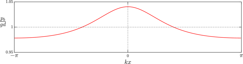
(a)

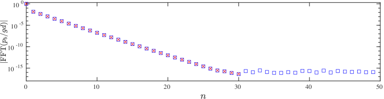
(b)

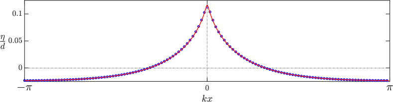
(c)

Figure 1. Example of surface recovery for $\omega\sqrt{d/g}=-1.7$, $H/d=0.14$ and $L/0pt=2\pi$: (a) pressure at the bottom; (b) Fourier spectrum extracted from bottom pressure (blue squares) and fitted harmonics used for the reconstruction (red crosses); (c) recovered wave profile (red line) versus exact surface profile (blue circles).

The numerical procedure consists in solving simultaneously the nonlinear set of equations (30), (5), (34), (35) (and the ones at $x_{0}$) to recover the surface wave profile and related parameters. To this end, we use an iterative root-finding algorithm (the built-in function fsolve in Matlab) supplemented with initial values given by the linear theory [19]. When needed, $\eta_{x}$ is computed directly from its explicit expression (31).

7. Example

In order to validate our procedure, we computed exact rotational waves with an accurate numerical algorithm similar to that of [16]. We then obtained bottom pressures that are considered the ‘measured’ ones from which the free surface and vorticity are recovered. Throughout the procedure, we monitor the convergence of our iterative algorithm using a tolerance of $10^{-12}$. When converged, the numerical solution is compared with the exact surface wave profile $\eta^{\textrm{ex}}$ and vorticity $\omega^{\textrm{ex}}$.

For waves of relatively small amplitudes, as well as small $\omega$, we witness a rapid convergence of the recovery procedure described above. The numerical errors of the recovered surface and vorticity are, respectively, $\epsilon_{\eta}=\lVert\eta-\eta^{\textrm{ex}}\rVert_{\infty}<10^{-8}$ and $\epsilon_{\omega}=\lvert\omega-\omega^{\textrm{ex}}\rvert<10^{-6}$. This excellent agreement is reached with as few as $N=5$ harmonics when considering the pressure Fourier expansion. However, for steady rotational waves with a steeper profile (thus departing from linear theory), the procedure naturally requires a larger number of harmonics.

Here, we illustrate our surface wave recovery procedure with numerical examples depicted in Figures 1 and 2 for a domain of size $L/d=2\pi$ (rather deep water for which surface recovery is a priori difficult). For our first example, we examine a steep wave with negative vorticity $\omega\sqrt{d/g}=-1.7$. Although the steep wave in figure 1c would appear to be quite challenging to compute, we still recover the correct surface profile using $N=30$ harmonics in our Fourier expansion (c.f. panel 1b), with the recovered solutions showing an excellent agreement with the exact data ($\epsilon_{\eta}\approx 10^{-4}$ and $\epsilon_{\omega}\approx 10^{-4}$).

For the second case of interest (Figure 2), we take the positive vorticity $\omega\sqrt{0pt/g}=3$. This value is greater than that predicated by linear wave theory for the existence of critical layers. Indeed, linear waves with $c_{0}>0$ never allow for stagnation points when $\omega<0$, while they contain stagnation points for $\omega>0$ iff $\tanh(kd)/kd\leq\omega^{2}d/(g+\omega^{2}d)$ [15, 16]. This example is of special interest because it involves three stagnation points per wavelength: two at the bottom (about half way between crests and troughs) and one within the fluid (under the crests), c.f. Figure 14a of [16]. The surface recovery still works relatively well in this case; taking $N=20$ Fourier modes, errors are $\epsilon_{\eta}\approx 10^{-3}$ and $\epsilon_{\omega}\approx 10^{-4}$ (see Figure 2).

We observe from panel 1a that the bottom pressure distribution for our choice of wave configuration displays a monotonic increase between trough and crest, which is not matched by that illustrated in panel 2a. This is not an artefact solely of the difference in signs of the vorticities, but rather also their magnitudes — an examination of explicit linear solutions for water waves with constant vorticity [2] illustrates the richness in behaviour of the pressure fluctuations even for small amplitude waves, both with regard to its monotonicity properties, and the location of its extrema. For nonlinear waves, the precise qualitative behaviour of the bottom pressure fluctuations due to wave motion (and the location of its extrema) was only recently rigorously established for irrotational periodic waves in [12], and there are presently no similarly rigorous mathematical results for nonlinear waves with constant vorticity. It is clear from panels 1a and 2a that considerable insight into this matter can be gained from a numerical approach.

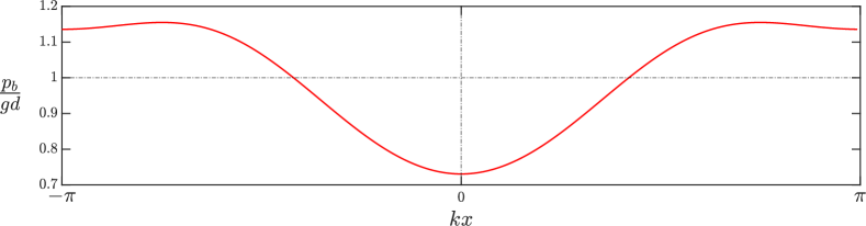
(a)

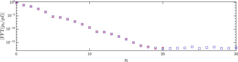
(b)

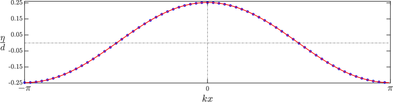
(c)

Figure 2. Same as Figure 1 for the case $\omega\sqrt{0pt/g}=3$, $H/d=0.5$ and $L/0pt=2\pi$.

8. Discussion

In this paper, we have presented a procedure for recovering fully nonlinear wave surface profiles from bottom pressure measurements for flows with constant vorticity. The theoretical basis for this procedure involves a reformulation in terms of holomorphic functions $\mathfrak{P}$ and $\mathfrak{Q}$, respectively introduced in [7] and [3], followed by a numerical implementation scheme. We have demonstrated the efficiency of this approach for different flow regimes, including one which presents stagnation points in the fluid body (an archetypical feature of waves with constant vorticity). For future work, it would be interesting to expand our approach to incorporate variable vorticity. Additionally, the question remains open as to whether our approach can be adapted to recover waves which exhibit overhanging profiles.

Funding. Joris Labarbe has been supported by the French government, through the $\mbox{UCA}^{\mbox{\tiny JEDI}}$ Investments in the Future project managed by the National Research Agency (ANR) with the reference number ANR-15-IDEX-01. David Henry acknowledges the support of the Science Foundation Ireland (SFI) under the grant SFI 21/FFP-A/9150.

Declaration of interests. The authors report no conflict of interest.

References

- [1] R. Aris, Vectors, tensors and basic equations of fluid mechanics, Dover, 1962.
- [2] O. Brink-Kjær, Gravity waves on a current: The influence of vorticity, a sloping bed, and dissipation, Institute of Hydrodynamics and Hydraulic Engineering, (ISVA), no. 12, Technical University of Denmark, 1976, pp. 1–137.
- [3] D. Clamond, New exact relations for easy recovery of steady wave profiles from bottom pressure measurements, J. Fluid Mech. 726 (2013), 547–558.
- [4] by same author, Remarks on Bernoulli constants, gauge conditions and phase velocities in the context of water waves, App. Math. Lett. 74 (2017), 114–120.
- [5] by same author, New exact relations for steady irrotational two-dimensional gravity and capillary surface waves, Phil. Trans. R. Soc. A 376 (2018), no. 2111, 20170220.
- [6] D. Clamond and E. Barthélémy, Experimental determination of the phase shift in the Stokes wave – solitary wave interaction, C. R. Ac. Sci. Paris IIb 320 (1995), no. 6, 277–280.
- [7] D. Clamond and A. Constantin, Recovery of steady periodic wave profiles from pressure measurements at the bed, J. Fluid Mech. 714 (2013), 463–475.
- [8] D. Clamond and D. Dutykh, Accurate fast computation of steady two-dimensional surface gravity waves in arbitrary depth, J. Fluid Mech. 844 (2018), 491–518.
- [9] D. Clamond and D. Henry, Extreme water-wave profile recovery from pressure measurements at the seabed, J. Fluid Mech. 903 (2020), R3, 12.
- [10] A. Constantin, Nonlinear water waves with applications to wave-current interactions and tsunamis, CBMS-NSF Regional Conference Series in Applied Mathematics, vol. 81, SIAM, Philadelphia, PA, 2011.
- [11] by same author, On the recovery of solitary wave profiles from pressure measurements, J. Fluid Mech. 699 (2012), 376–384.
- [12] by same author, Extrema of the dynamic pressure in an irrotational regular wave train, Physics of Fluids 28 (2016), no. 11, 113604.
- [13] A. Constantin, W. Strauss, and E. Varvaruca, Global bifurcation of steady gravity water waves with critical layers, Acta Math. 217 (2016), no. 2, 195–262.
- [14] by same author, Large-amplitude steady downstream water waves, Comm. Math. Phys. 387 (2021), no. 1, 237–266.
- [15] A. Constantin and E. Varvaruca, Steady periodic water waves with constant vorticity: regularity and local bifurcation, Arch. Ration. Mech. Anal. 199 (2011), no. 1, 33–67.
- [16] A. T. Da Silva and D. H. Peregrine, Steep, steady surface waves on water of finite depth with constant vorticity, J. Fluid Mech. 195 (1988), 281–302.
- [17] D. Henry, On the pressure transfer function for solitary water waves with vorticity, Math. Ann. 357 (2013), no. 1, 23–30.
- [18] D. Henry and G. P. Thomas, Prediction of the free-surface elevation for rotational water waves using the recovery of pressure at the bed, Philos. Trans. Roy. Soc. A 376 (2018), no. 2111, 20170102, 21.
- [19] N. Kishida and J. Sobey, Stokes theory for waves on linear shear current, J. Engin. Mech. 114 (1988), no. 8, 1317–1334.
- [20] H. Okamoto and M. Shoji, The mathematical theory of permanent progressive water-waves, Advanced Series in Nonlinear Dynamics, vol. 20, World Scientific Publishing Co., Inc., River Edge, NJ, 2001.
- [21] K. L. Oliveras, V. Vasan, B. Deconinck, and D. Henderson, Recovering the water-wave profile from pressure measurements, SIAM J. Appl. Math. 72 (2012), no. 3, 897–918.
- [22] G.P. Thomas and G. Klopman, Wave-current interactions in the nearshore region, Gravity waves in water of finite depth (J. N. Hunt, ed.), Advances in Fluid Mechanics, Computational Mechanics Publications, 1997, pp. 255–319.