Classification Schemes for the Radar Reference Window: Design and Comparisons

Abstract

In this paper, we address the problem of classifying data within the radar reference window in terms of statistical properties. Specifically, we partition these data into statistically homogeneous subsets by identifying possible clutter power variations with respect to the cells under test (accounting for possible range-spread targets) and/or clutter edges. To this end, we consider different situations of practical interest and formulate the classification problem as multiple hypothesis tests comprising several models for the operating scenario. Then, we solve the hypothesis testing problems by resorting to suitable approximations of the model order selection rules due to the intractable mathematics associated with the maximum likelihood estimation of some parameters. Remarkably, the classification results provided by the proposed architectures represent an advanced clutter map since, besides the estimation of the clutter parameters, they contain a clustering of the range bins in terms of homogeneous subsets. In fact, such information can drive the conventional detectors towards more reliable estimates of the clutter covariance matrix according to the position of the cells under test. The performance analysis confirms that the conceived architectures represent a viable means to recognize the scenario wherein the radar is operating at least for the considered simulation parameters.

I Introduction

Target detection is a task that is ubiquitous in radar systems [1, 2, 3] and, due to its vital importance, it has attracted and continues to attract the attention of the radar community. More importantly, the advances in technology and the consequent spread of radars in several aspects of real life have led to more challenging operating scenarios that might no longer meet the design requirements of the classical detection architectures. In fact, the most common assumption is that the statistical characterization of the interference (i.e., clutter and noise) in secondary data, collected in the vicinity of the Cell Under Test (CUT), is the same as that in the CUT (homogeneous environment) [4, 5, 6, 7, 8, 9, 10, 11, 12, 13, 14, 15, 16, 17, 18, 19, 20, 21, 22, 23, 24, 25, 26, 27, 28, and references therein]. The first contributions in the context of space-time adaptive processing where the homogeneous environment is exploited at the design stage, are [4, 5, 6]. Actually, they paved the way for a plethora of other works based upon the same interference model but with additional design assumptions accounting for different situations of practical value. For instance, when the target signature experiences a slightly different direction from the nominal one due to imperfect modeling of the nominal steering vector, calibration/beampointing errors, or target position within the mainlobe, the subspace paradigm represents an effective means to face these situations as shown in [7, 14, 20, 29, 19]. Another useful signal model in radar arises from the fact that, depending on the system range resolution, a target can be resolved into multiple scatterers that are distributed over the range leading to the so-called range-spread or extended target model [8, 14, 20, 15, 17, 18]. Actually, this model comes also in handy to account for the possible spillover of target energy between adjacent range bins [26] or when the system oversamples the backscattered echoes [16]. Finally, it is worth mentioning that specific structures for the clutter covariance matrix can improve the estimation quality of the unknown parameters. As a matter of fact, a radar system equipped with a symmetrically spaced linear array or using symmetrically spaced pulse trains could collect data statistically symmetric in forward and reverse directions. This results into an interference covariance matrix which shares a so-called “doubly” symmetric form, i.e., Hermitian about its principal diagonal and persymmetric about its cross diagonal. The number of unknowns associated with a persymmetric covariance matrix is lower than that for the general Hermitian case leading to enhanced estimation and, hence, detection performance as shown in [11, 25, 28, 10]. Another useful covariance structure is related to ground clutter whose power spectral density is symmetric with respect to zero-Doppler frequency. As a result, the associated covariance matrix is real symmetric [10, 13, 22].

However, in many situations of practical interest, the homogeneous environment does not represent a good scenario approximation due to the presence of clutter regions with different properties leading to architectures with poor detection performance and/or that cannot keep under control the number of false alarms [30, 31]. Thus, it appears clear that new insights are necessary and more articulated models have to be designed starting from the well-known partially-homogeneous environment [32, 33, 34, 35, 36, 20, 37, 38, 39, 40, 41], where interference in the secondary data shares the same structure of the covariance matrix as in the CUT but a different power level, up to the most general case where secondary data are heterogeneous in terms of statistical properties. A widely used clutter model for heterogeneous environments assumes that each range bin shares the same structure for the clutter covariance matrix but different scaling factors that are representative of different clutter types (and reflectivity). The interested reader is referred to [42, 43, 44, 45, and references therein] for examples related to this model.

From the above discussion it is quite evident that most of the existing adaptive detection architectures are devised assuming a specific operating environment and clutter model. Therefore, clutter classification becomes a relevant issue to select the detector and/or training data that are perfectly matched to the current operating scenario. Such a choice would be a key factor for achieving higher performance. In this context, pioneering solutions based upon the neural networks can be found in [46, 47], where the classifier distinguishes several types of environment returns including birds, weather, ground, and sea clutter. The same problem is recently addressed in [48] by means of an algorithm based upon the support vector machine [49]. Clutter classification can be also accomplished in terms of covariance structure, which is related to specific clutter properties and types, as shown in [50, 51], where the so-called Model Order Selection (MOS) rules [52, 53] are applied to deal with multiple (possibly nested) hypotheses. In [54] the above approach is extended to the case of heterogeneous environments. The common assumption behind these important contributions is that data under test are characterized by the same covariance structure as also in [55] where a binary hypothesis test is solved to discriminate between the homogeneous and the heterogeneous (with respect to the clutter power) environment. In [56], the aforementioned assumption is no longer used at the design stage and an architecture grounded on the Generalized Likelihood Ratio Test (GLRT) is devised to declare the presence of a possible clutter edge within a window of consecutive range bins. The extension of [56] to the case of specific covariance structures can be found in [57]. In [58], range bin clustering algorithms based upon clutter covariance matrix are conceived to partition the entire region of interest into homogeneous subsets of (not necessarily contiguous) range cells. Finally, it is worth mentioning the knowledge-aided paradigm as another effective means to guide the system towards reliable clutter parameter estimates [59, 60, 61]. It consists in accounting for all the available a priori informations about the region of interest to exclude inhomogeneities from the computation of the sample covariance matrix [30].

All the above examples show that the a priori knowledge about the radar operating environment is a precious information that can be suitably exploited to come up with reliable estimates of the clutter parameters. Besides, highly reliable estimates allow for an enhanced adaptivity with respect to the clutter in the CUT improving the detection capabilities of the system. From this perspective, in the present paper, we focus on the traditional reference window used to collect secondary data and formed by the CUT, lagging plus leading windows, and guard cells [1]. Then, all these data are used to conceive innovative classification schemes capable of identifying different situations of practical interest. Since two hypotheses only are not enough to account for all such situations, it naturally follows that this problem cannot be modeled in terms of a conventional binary hypothesis test as in [55, 56, 57] but a multiple hypothesis test is required. As a matter of fact, each hypothesis corresponds to one of the following scenarios: primary and secondary data are statistically homogeneous; clutter in primary data have a different power level with respect to that in secondary data (partially-homogeneous environment); finally, one or two clutter edges are present in the secondary data unlike [56, 57], where only one clutter edge is assumed.

Three remarks are now in order. First, the partially-homogeneous model developed in this paper is different from the conventional one since the overall covariance matrix originates from the sum of thermal noise and clutter components. Second, training data partitioning is performed with the constraint that the homogeneous regions are formed by contiguous range bins unlike [58] where misclassification errors within a given region might occur. Third, from an operating point of view, a radar system can perform a preliminary scan by moving the reference window over the region of interest to build up a kind of clutter map. This map can be used for secondary data selection once the detection function is active.

Thus, as stated before, the classification problem at hand is formulated in terms of a multiple hypothesis test and solved by resorting to decision schemes relying on the MOS rules. Such a design choice is dictated by the fact that in the presence of nested hypotheses the likelihood function monotonically increases with the number of parameters. Otherwise stated, the Maximum Likelihood Approach (MLA) is inclined to select the model with the highest number of unknown parameter [52, 62]. In order to contrast this natural inclination of the MLA in the presence of nested hypotheses, the MOS rules exploit suitable penalty terms that promote low-dimensional models [52, 62]. In fact, the general structure of a MOS decision statistic is given by the negative of the compressed log-likelihood function under a specific model order plus a penalty term that depends on the number of unknown parameters under that model. Here, “compressed” means that the unknown parameters are replaced by their respective maximum likelihood estimates (MLEs). The selection of the model order is accomplished by minimizing the above structure with respect to the number of parameters (model order). The herein considered MOS rule are the Akaike Information Criterion (AIC), the Generalized Information Criterion (GIC), and the Bayesian Information Criterion (BIC). However, in this work, we derive suitable approximations of the MOS rules due to the difficult mathematics related to the maximum likelihood estimation of some parameters. In addition, we consider two models for the clutter covariance matrices which differ in the power variation over the range bins (a point better explained in Section II). Finally, the classification capabilities of the proposed architectures are assessed using synthetic data. The illustrative examples reveal that they can return the correct operating hypothesis with high probability at least for the considered parameter values.

The remainder of this paper is organized as follows. The next section provides a formal statement of the problem at hand along with the preliminary definitions that will be used in the ensuing derivations. Section III contains the design of the classification architectures, whereas Section IV shows the classification performances through numerical examples. Concluding remarks and hints for future research lines are discussed in Section V. Finally, some mathematical derivations are confined to the appendix.

I-A Notation

In the sequel, vectors (matrices) are denoted by boldface lower (upper) case letter. Superscripts $(\cdot)^{T}$ and $(\cdot)^{\dagger}$ denote transpose and complex conjugate transpose, respectively. We denote by ${\mbox{\boldmath$S$}}(i,j)$ the $(i,j)$th element in the matrix $S$. $\mathds{R}^{m\times n}$ and $\mathds{C}^{m\times n}$ are real and complex matrix spaces of dimension $m\times n$. Given a vector ${\mbox{\boldmath$x$}}\in\mathds{C}^{N\times 1}$, we denote by $diag({\mbox{\boldmath$x$}})\in\mathds{C}^{N\times N}$ a diagonal matrix whose nonzero entries are the elements of $x$. $I$ stands for an identity matrix with suitable dimension. The notation $\sim$ means “be distributed as”. $\mbox{$\mathcal{C}$}\mbox{$\mathcal{N}$}_{N}(\bm{\mu},{\mbox{\boldmath$X$}})$ denotes the $N$-dimensional circular complex Gaussian distribution with mean $\bm{\mu}$ and covariance matrix $X$. $\succ$ denotes positive-definite and $\prec$ denotes negative-definite. $\det(\cdot)$ represents the determinant of a matrix and $|\cdot|$ is the modulus of a scalar. $\mbox{Tr}(\cdot)$ denotes the trace of a square matrix. $\jmath=\sqrt{-1}$ and $U(0,1)$ the uniformly distributed random variable on the interval from 0 to 1.

II Problem Formulation and Preliminary Definitions

Consider a radar system equipped with $N\geq 2$ space and/or time channels illuminating the surveillance area. The measurements of the backscattered echoes from the range cells are properly processed and sampled to form $N$-dimensional complex vectors. Now, notice that when a point-like target is present in a given range bin, the range cells in the neighborhood of the latter might be contaminated by target components (energy spillover [26]); the same effect is also observed in the presence of range-spread targets due to an enhanced range resolution [8]. Thus, we assume that the system performs the decision over a set of primary data denoted by ${\mbox{\boldmath$z$}}_{k}\in\mathds{C}^{N\times 1}$, $k=1,\ldots,K_{P}$, corresponding to ${K_{P}}$ consecutive CUTs. Furthermore, we denote by ${\mbox{\boldmath$r$}}_{k}\in\mathds{C}^{N\times 1}$, $k=1,\ldots,K_{S}$, a set of secondary data gathered from the leading and lagging window [1] in the proximity of the CUTs. Finally, we assume that before testing for the presence of a target the system performs a preliminary scan of the entire region of interest to classify the scenario and build up a kind of clutter map [63, 64]. For this reason, at the design stage, all data are assumed free of target components as well as independent and identically distributed circularly symmetric complex Gaussian random vectors with zero mean and positive definite covariance matrix.

Moreover, we consider two situations of clutter covariance variation and accordingly formulate two classification problems, where the second one accounts for a more general scenario. Specifically, the first scenario assumes that primary and secondary data share the same covariance matrix except for scaling factors representative of different power levels. Notice that in this case, all of the secondary data can be used in the detection stage to estimate the covariance structure. The second scenario considers the case that the background experiences extremely serious fluctuations caused by, for example, a drastic variation of terrain type, multiple interferences, or other extreme transitions, and the variation of the clutter power and subspace is thus arbitrary.

Let us start from the first scenario and consider the following configurations (or hypotheses):

• the homogeneous environment ($H_{\text{I},0}$), where the interference component in the primary and secondary data share the same statistical characterization [4, 5, 10], as illustrated in Fig. 1;

• the well-known partially-homogeneous environment ($H_{\text{I},1}$), where clutter in the primary and secondary data share the same clutter covariance structure but different clutter power [33, 65] as illustrated in Fig. 2;

• an intermediate heterogeneous environment where secondary data contains only one clutter edge coming from either the lagging or the leading window ($H_{\text{I},2}$) [56], as illustrated in Fig. 3(a);

• an intermediate heterogeneous environment with a clutter edge present in both the leading and lagging window ($H_{\text{I},3}$) as illustrated in Fig. 3(b).

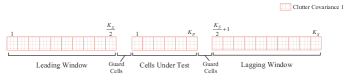
Figure 1: Diagrams of homogeneous environments

Figure 2: Diagrams of partially-homogeneous environments

In Fig. 3, Clutter Covariance 1, 2, and 3 differ only in terms of clutter power. Therefore, the classification problem for radar scenarios can be formulated in terms of the following multiple hypothesis test

$$\left\{\begin{array}[]{lll}H_{\text{I},0}:\left\{\begin{array}[]{lll}{\mbox{\boldmath$z$}}_{k}\sim\mbox{$\mathcal{C}$}\mbox{$\mathcal{N}$}_{N}(\textbf{0},\sigma^{2}{\mbox{\boldmath$I$}}+{\mbox{\boldmath$M$}}),\\ k=1,\ldots,{K_{P}},\\ {\mbox{\boldmath$r$}}_{k}\sim\mbox{$\mathcal{C}$}\mbox{$\mathcal{N}$}_{N}(\textbf{0},\sigma^{2}{\mbox{\boldmath$I$}}+{\mbox{\boldmath$M$}}),\\ k=1,\ldots,K_{S},\\ \end{array}\right.\\ \vspace{-2mm}\\ H_{\text{I},1}:\left\{\begin{array}[]{lll}{\mbox{\boldmath$z$}}_{k}\sim\mbox{$\mathcal{C}$}\mbox{$\mathcal{N}$}_{N}(\textbf{0},\sigma^{2}{\mbox{\boldmath$I$}}+{\mbox{\boldmath$M$}}),\\ k=1,\ldots,{K_{P}},\\ {\mbox{\boldmath$r$}}_{k}\sim\mbox{$\mathcal{C}$}\mbox{$\mathcal{N}$}_{N}(\textbf{0},\sigma^{2}{\mbox{\boldmath$I$}}+{\mbox{\boldmath$M$}}_{1}),\\ k=1,\ldots,K_{S},\\ \end{array}\right.\\ \vspace{-2mm}\\ H_{\text{I},2}:\left\{\begin{array}[]{lll}{\mbox{\boldmath$z$}}_{k}\sim\mbox{$\mathcal{C}$}\mbox{$\mathcal{N}$}_{N}(\textbf{0},\sigma^{2}{\mbox{\boldmath$I$}}+{\mbox{\boldmath$M$}}),\\ k=1,\ldots,{K_{P}},\\ {\mbox{\boldmath$r$}}_{k}\sim\mbox{$\mathcal{C}$}\mbox{$\mathcal{N}$}_{N}(\textbf{0},\sigma^{2}{\mbox{\boldmath$I$}}+{\mbox{\boldmath$M$}}),\\ k=1,\ldots,K_{\text{I},1},\\ {\mbox{\boldmath$r$}}_{k}\sim\mbox{$\mathcal{C}$}\mbox{$\mathcal{N}$}_{N}(\textbf{0},\sigma^{2}{\mbox{\boldmath$I$}}+{\mbox{\boldmath$M$}}_{2}),\\ k=K_{\text{I},1}+1,\ldots,K_{S},\\ \end{array}\right.\\ \vspace{-2mm}\\ H_{\text{I},3}:\left\{\begin{array}[]{lll}{\mbox{\boldmath$z$}}_{k}\sim\mbox{$\mathcal{C}$}\mbox{$\mathcal{N}$}_{N}(\textbf{0},\sigma^{2}{\mbox{\boldmath$I$}}+{\mbox{\boldmath$M$}}),\\ k=1,\ldots,{K_{P}},\\ {\mbox{\boldmath$r$}}_{k}\sim\mbox{$\mathcal{C}$}\mbox{$\mathcal{N}$}_{N}(\textbf{0},\sigma^{2}{\mbox{\boldmath$I$}}+{\mbox{\boldmath$M$}}_{3}),\\ k=1,\ldots,K_{\text{I},2},\\ {\mbox{\boldmath$r$}}_{k}\sim\mbox{$\mathcal{C}$}\mbox{$\mathcal{N}$}_{N}(\textbf{0},\sigma^{2}{\mbox{\boldmath$I$}}+{\mbox{\boldmath$M$}}),\\ k=K_{\text{I},2}+1,\ldots,K_{\text{I},3},\\ {\mbox{\boldmath$r$}}_{k}\sim\mbox{$\mathcal{C}$}\mbox{$\mathcal{N}$}_{N}(\textbf{0},\sigma^{2}{\mbox{\boldmath$I$}}+{\mbox{\boldmath$M$}}_{4}),\\ k=K_{\text{I},3}+1,\ldots,K_{S},\\ \end{array}\right.\end{array}\right.$$ (1)

where $\sigma^{2}{\mbox{\boldmath$I$}}$ is the thermal noise component with $\sigma^{2}>0$ the unknown noise power level; ${\mbox{\boldmath$M$}}=\bm{U}\bm{\Lambda}\bm{U}^{\dagger}\in\mathds{C}^{N\times N}$ is the positive semidefinite clutter covariance matrix of the primary data where $\bm{\Lambda}=diag\left(\lambda_{1},\ldots,\lambda_{r},0,\ldots,0\right)$, $\lambda_{1}\geq\ldots\geq\lambda_{r}>0$, contains the eigenvalues of $M$ with $r<N$ the rank for the moment assumed known, $U$ is the unitary matrix of the corresponding eigenvectors; $K_{P}>r$, $K_{S}>r$ with $K_{S}$ an even number, and we denote by $K_{\text{I},1}\in\left\{r,\ldots,K_{S}-r\right\}$, $K_{\text{I},2}\in\left\{r,\ldots,\frac{K_{S}}{2}\right\}$, and $K_{\text{I},3}\in\left\{\frac{K_{S}}{2}+1,\ldots,K_{S}-r\right\}$ the unknown positions of the clutter power transitions within the leading and lagging windows under $H_{\text{I},2}$ and $H_{\text{I},3}$, respectively. In order to better understand the clutter characteristics under $H_{\text{I},2}$ and $H_{\text{I},3}$, it is important to highlight that we assume that in the spatial proximity of the CUTs there exist range bins that share the same clutter power level as that in the primary data. As for ${\mbox{\boldmath$M$}}_{l}\in\mathds{C}^{N\times N}$, $l=1,\ldots,4$, they are defined as ${\mbox{\boldmath$M$}}_{l}={\mbox{\boldmath$U$}}\bm{\Gamma}_{l}\bm{\Lambda}\bm{\Gamma}_{l}{\mbox{\boldmath$U$}}^{\dagger}$, where $\bm{\Gamma}_{l}=diag(\sqrt{\gamma_{1,l}},\ldots,\sqrt{\gamma_{r,l}},0,\ldots,0)$, $\gamma_{1,l}\geq\ldots\geq\gamma_{r,l}>0$, is representative of possible power variations of the clutter along different directions. It is important to notice that these covariance structures model situations where the spatial distribution of the clutter remains approximately unaltered over the range (clutter scatterers respond from a given set of directions) whereas clutter reflectivity might change over the range leading to different power levels associated with the main echoes’ directions.

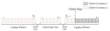
(a) Intermediate heterogeneous environment with one clutter edge

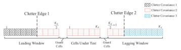
(b) Intermediate heterogeneous environment with two clutter edges

Figure 3: Diagrams of intermediate heterogeneous environments

For notation convenience, let us denote by ${\mbox{\boldmath$Z$}}_{P}=\left[{\mbox{\boldmath$z$}}_{1},\ldots,{\mbox{\boldmath$z$}}_{K_{P}}\right]\in\mathds{C}^{N\times{K_{P}}}$, ${\mbox{\boldmath$Z$}}_{S}=\left[{\mbox{\boldmath$r$}}_{1},\ldots,{\mbox{\boldmath$r$}}_{K_{S}}\right]\in\mathds{C}^{N\times K_{S}}$, and ${\mbox{\boldmath$Z$}}=\left[{\mbox{\boldmath$Z$}}_{P},{\mbox{\boldmath$Z$}}_{S}\right]\in\mathds{C}^{N\times({K_{P}}+K_{S})}$ the overall data set. Based upon the above assumptions, the probability density function (PDF) of $Z$ under $H_{\text{I},m}$, $m=0,\ldots,3$, namely $f_{\text{I},m}({\mbox{\boldmath$Z$}};\bm{\theta}_{m})$ can be expressed as $f_{\text{I},m}({\mbox{\boldmath$Z$}};\bm{\theta}_{m})=f_{P}({\mbox{\boldmath$Z$}}_{P};\sigma^{2},{\mbox{\boldmath$M$}})f_{S_{\text{I},m}}({\mbox{\boldmath$Z$}}_{S};\bm{\theta}_{m})$, where

$$\begin{cases}f_{P}({\mbox{\boldmath$Z$}}_{P};\sigma^{2},{\mbox{\boldmath$M$}})=\left[\frac{\exp{\left\{-\frac{1}{K_{P}}\sum_{k=1}^{K_{P}}{\mbox{\boldmath$z$}}_{k}^{\dagger}(\sigma^{2}\bm{I}+\bm{M})^{-1}{\mbox{\boldmath$z$}}_{k}\right\}}}{\pi^{N}\det(\sigma^{2}\bm{I}+\bm{M})}\right]^{K_{P}},\\ f_{S_{\text{I},0}}({\mbox{\boldmath$Z$}}_{S};\bm{\theta}_{0})=\left[\frac{\exp{\left\{-\frac{1}{K_{S}}\sum_{k=1}^{K_{S}}{\mbox{\boldmath$r$}}_{k}^{\dagger}(\sigma^{2}\bm{I}+\bm{M})^{-1}{\mbox{\boldmath$r$}}_{k}\right\}}}{\pi^{N}\det(\sigma^{2}\bm{I}+\bm{M})}\right]^{K_{S}},\\ f_{S_{\text{I},1}}({\mbox{\boldmath$Z$}}_{S};\bm{\theta}_{1})=\left[\frac{\exp{\left\{-\frac{1}{K_{S}}\sum_{k=1}^{K_{S}}{\mbox{\boldmath$r$}}_{k}^{\dagger}(\sigma^{2}\bm{I}+\bm{M}_{1})^{-1}{\mbox{\boldmath$r$}}_{k}\right\}}}{\pi^{N}\det(\sigma^{2}\bm{I}+\bm{M}_{1})}\right]^{K_{S}},\\ f_{S_{\text{I},2}}({\mbox{\boldmath$Z$}}_{S};\bm{\theta}_{2})=\left[\frac{\exp{\left\{-\frac{1}{K_{\text{I},1}}\sum_{k=1}^{K_{\text{I},1}}{\mbox{\boldmath$r$}}_{k}^{\dagger}(\sigma^{2}\bm{I}+\bm{M})^{-1}{\mbox{\boldmath$r$}}_{k}\right\}}}{\pi^{N}\det(\sigma^{2}\bm{I}+\bm{M})}\right]^{K_{\text{I},1}}\\ \qquad\times\left[\frac{\exp{\left\{-\frac{1}{K_{S}-K_{\text{I},1}}\sum_{k=K_{\text{I},1}+1}^{K_{S}}{\mbox{\boldmath$r$}}_{k}^{\dagger}(\sigma^{2}\bm{I}+\bm{M}_{2})^{-1}{\mbox{\boldmath$r$}}_{k}\right\}}}{\pi^{N}\det(\sigma^{2}\bm{I}+\bm{M}_{2})}\right]^{K_{S}-K_{\text{I},1}},\\ f_{S_{\text{I},3}}({\mbox{\boldmath$Z$}}_{S};\bm{\theta}_{3})=\left[\frac{\exp{\left\{-\frac{1}{K_{\text{I},2}}\sum_{k=1}^{K_{\text{I},2}}{\mbox{\boldmath$r$}}_{k}^{\dagger}(\sigma^{2}\bm{I}+\bm{M}_{3})^{-1}{\mbox{\boldmath$r$}}_{k}\right\}}}{\pi^{N}\det(\sigma^{2}\bm{I}+\bm{M}_{3})}\right]^{K_{\text{I},2}}\\ \qquad\times\left[\frac{\exp{\left\{-\frac{1}{K_{\text{I},3}-K_{\text{I},2}}\sum_{k=K_{\text{I},2}+1}^{K_{\text{I},3}}{\mbox{\boldmath$r$}}_{k}^{\dagger}(\sigma^{2}\bm{I}+\bm{M})^{-1}{\mbox{\boldmath$r$}}_{k}\right\}}}{\pi^{N}\det(\sigma^{2}\bm{I}+\bm{M})}\right]^{K_{\text{I},3}-K_{\text{I},2}}\\ \qquad\times\left[\frac{\exp{\left\{-\frac{1}{K_{S}-K_{\text{I},3}}\sum_{k=K_{\text{I},3}+1}^{K_{S}}{\mbox{\boldmath$r$}}_{k}^{\dagger}(\sigma^{2}\bm{I}+\bm{M}_{4})^{-1}{\mbox{\boldmath$r$}}_{k}\right\}}}{\pi^{N}\det(\sigma^{2}\bm{I}+\bm{M}_{4})}\right]^{K_{S}-K_{\text{I},3}},\end{cases}$$ (2)

with

$$\bm{\theta}_{0}=\left[\sigma^{2},\bm{\nu}^{T}({\mbox{\boldmath$M$}})\right]^{T},\bm{\theta}_{1}=\left[\bm{\theta}_{0}^{T},\bm{\nu}^{T}({\mbox{\boldmath$M$}}_{1})\right]^{T},$$

$$\bm{\theta}_{2}=\left[\bm{\theta}_{0}^{T},K_{\text{I},1},\bm{\nu}^{T}({\mbox{\boldmath$M$}}_{2})\right]^{T},\qquad\qquad\qquad\quad$$

$$\bm{\theta}_{3}=\left[\bm{\theta}_{0}^{T},K_{\text{I},2},K_{\text{I},3},\bm{\nu}^{T}({\mbox{\boldmath$M$}}_{3}),\bm{\nu}^{T}({\mbox{\boldmath$M$}}_{4})\right]^{T},\ \$$ (3)

and $\bm{\nu}({\mbox{\boldmath$M$}})$ the vector-valued function selecting the distinct entries of $M$.

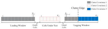
Figure 4: Heterogeneous environment with one clutter edge

In the second scenario, we assume that the variation of the clutter power and subspace over the range is arbitrary. Specifically, we modify the hypothesis test (1) by adopting a different covariance variation model that does not assume any relationship among the covariances. Moreover, we introduce an additional hypothesis, $H_{\text{II},4}$ say, where the data in lagging and leading windows belong to two separated and different clutter regions whose properties are also different from those of the clutter in the primary data, as depicted in Fig. 4. Notice that the situation represented by $H_{\text{II},4}$ is not considered in the first scenario since, when secondary data are partitioned into different clutter regions, the estimation quality of some parameters can seriously degrade due to the specific constraints of the first covariance model. Specifically, under such assumptions, they can impair the estimation performance in the presence of a limited amount of data characterized by $M$.

With the above remarks in mind, the second classification problem can be formulated as the following multiple hypothesis testing problem

$$\left\{\begin{array}[]{lll}H_{\text{II},0}:\left\{\begin{array}[]{lll}{\mbox{\boldmath$z$}}_{k}\sim\mbox{$\mathcal{C}$}\mbox{$\mathcal{N}$}_{N}(\textbf{0},\sigma^{2}{\mbox{\boldmath$I$}}+{\mbox{\boldmath$M$}}),\\ k=1,\ldots,{K_{P}},\\ {\mbox{\boldmath$r$}}_{k}\sim\mbox{$\mathcal{C}$}\mbox{$\mathcal{N}$}_{N}(\textbf{0},\sigma^{2}{\mbox{\boldmath$I$}}+{\mbox{\boldmath$M$}}),\\ k=1,\ldots,K_{S},\\ \end{array}\right.\\ \vspace{-2mm}\\ H_{\text{II},1}:\left\{\begin{array}[]{lll}{\mbox{\boldmath$z$}}_{k}\sim\mbox{$\mathcal{C}$}\mbox{$\mathcal{N}$}_{N}(\textbf{0},\sigma^{2}{\mbox{\boldmath$I$}}+{\mbox{\boldmath$M$}}),\\ k=1,\ldots,{K_{P}},\\ {\mbox{\boldmath$r$}}_{k}\sim\mbox{$\mathcal{C}$}\mbox{$\mathcal{N}$}_{N}(\textbf{0},\sigma^{2}{\mbox{\boldmath$I$}}+{\mbox{\boldmath$R$}}_{1}),\\ k=1,\ldots,K_{S},\\ \end{array}\right.\\ \vspace{-2mm}\\ H_{\text{II},2}:\left\{\begin{array}[]{lll}{\mbox{\boldmath$z$}}_{k}\sim\mbox{$\mathcal{C}$}\mbox{$\mathcal{N}$}_{N}(\textbf{0},\sigma^{2}{\mbox{\boldmath$I$}}+{\mbox{\boldmath$M$}}),\\ k=1,\ldots,{K_{P}},\\ {\mbox{\boldmath$r$}}_{k}\sim\mbox{$\mathcal{C}$}\mbox{$\mathcal{N}$}_{N}(\textbf{0},\sigma^{2}{\mbox{\boldmath$I$}}+{\mbox{\boldmath$M$}}),\\ k=1,\ldots,K_{\text{II},1},\\ {\mbox{\boldmath$r$}}_{k}\sim\mbox{$\mathcal{C}$}\mbox{$\mathcal{N}$}_{N}(\textbf{0},\sigma^{2}{\mbox{\boldmath$I$}}+{\mbox{\boldmath$R$}}_{2}),\\ k=K_{\text{II},1}+1,\ldots,K_{S},\\ \end{array}\right.\\ \vspace{-2mm}\\ H_{\text{II},3}:\left\{\begin{array}[]{lll}{\mbox{\boldmath$z$}}_{k}\sim\mbox{$\mathcal{C}$}\mbox{$\mathcal{N}$}_{N}(\textbf{0},\sigma^{2}{\mbox{\boldmath$I$}}+{\mbox{\boldmath$M$}}),\\ k=1,\ldots,{K_{P}},\\ {\mbox{\boldmath$r$}}_{k}\sim\mbox{$\mathcal{C}$}\mbox{$\mathcal{N}$}_{N}(\textbf{0},\sigma^{2}{\mbox{\boldmath$I$}}+{\mbox{\boldmath$R$}}_{3}),\\ k=1,\ldots,K_{\text{II},2},\\ {\mbox{\boldmath$r$}}_{k}\sim\mbox{$\mathcal{C}$}\mbox{$\mathcal{N}$}_{N}(\textbf{0},\sigma^{2}{\mbox{\boldmath$I$}}+{\mbox{\boldmath$M$}}),\\ k=K_{\text{II},2}+1,\ldots,K_{\text{II},3},\\ {\mbox{\boldmath$r$}}_{k}\sim\mbox{$\mathcal{C}$}\mbox{$\mathcal{N}$}_{N}(\textbf{0},\sigma^{2}{\mbox{\boldmath$I$}}+{\mbox{\boldmath$R$}}_{4}),\\ k=K_{\text{II},3}+1,\ldots,K_{S},\\ \end{array}\right.\\ \vspace{-2mm}\\ H_{\text{II},4}:\left\{\begin{array}[]{lll}{\mbox{\boldmath$z$}}_{k}\sim\mbox{$\mathcal{C}$}\mbox{$\mathcal{N}$}_{N}(\textbf{0},\sigma^{2}{\mbox{\boldmath$I$}}+{\mbox{\boldmath$M$}}),\\ k=1,\ldots,{K_{P}},\\ {\mbox{\boldmath$r$}}_{k}\sim\mbox{$\mathcal{C}$}\mbox{$\mathcal{N}$}_{N}(\textbf{0},\sigma^{2}{\mbox{\boldmath$I$}}+{\mbox{\boldmath$R$}}_{5}),\\ k=1,\ldots,K_{\text{II},4},\\ {\mbox{\boldmath$r$}}_{k}\sim\mbox{$\mathcal{C}$}\mbox{$\mathcal{N}$}_{N}(\textbf{0},\sigma^{2}{\mbox{\boldmath$I$}}+{\mbox{\boldmath$R$}}_{6}),\\ k=K_{\text{II},4}+1,\ldots,K_{S},\\ \end{array}\right.\end{array}\right.$$ (4)

where ${\mbox{\boldmath$M$}}=\bm{U}\bm{\Lambda}\bm{U}^{\dagger}$ is the clutter covariance matrix of primary data, ${\mbox{\boldmath$R$}}_{l}=\bm{U}_{l}\bm{\Lambda}_{l}\bm{U}_{l}^{\dagger}$, $l=1,\ldots,6$, with $\bm{\Lambda}_{l}=diag\left(\lambda_{1,l},\ldots,\lambda_{r,l},0,\ldots,0\right)$, $\lambda_{1,l}\geq\ldots\geq\lambda_{r,l}>0$, containing the eigenvalues of ${\mbox{\boldmath$R$}}_{l}$, and ${\mbox{\boldmath$U$}}_{l}$ the unitary matrix of the corresponding eigenvectors. In (4), $H_{\text{II},0}$ is equivalent to $H_{\text{I},0}$, namely the homogeneous environment, whereas $H_{\text{II},1}$ is the totally heterogeneous environment where the covariance matrices of primary and secondary data are arbitrarily different except for the rank, $H_{\text{II},2}$ and $H_{\text{II},3}$ are the same configurations as $H_{\text{I},2}$ and $H_{\text{I},3}$, respectively, and $H_{\text{II},4}$ is the situation that a clutter edge is present under $H_{\text{II},1}$. $K_{\text{II},1}\in\left\{r,\ldots,K_{S}-r\right\}$, $K_{\text{II},2}\in\left\{r,\ldots,\frac{K_{S}}{2}\right\}$, $K_{\text{II},3}\in\left\{\frac{K_{S}}{2}+1,\ldots,K_{S}-r\right\}$, and $K_{\text{II},4}\in\left\{r,\ldots,K_{S}-r\right\}$ are the positions of the edges under $H_{\text{II},2}$, $H_{\text{II},3}$ and $H_{\text{II},4}$, respectively. It can be observed that, by solving (4), heterogeneous data sets are clustered into homogeneous subsets and only the subsets of secondary data which share the same clutter covariance matrix with primary data can be used for detection.

The PDF of $Z$ under $H_{\text{II},n}$, $n=0,\ldots,4$, namely $f_{\text{II},n}({\mbox{\boldmath$Z$}};\bm{\delta}_{n})$ can be expressed as $f_{\text{II},n}({\mbox{\boldmath$Z$}};\bm{\delta}_{n})=f_{P}({\mbox{\boldmath$Z$}}_{P};\sigma^{2},{\mbox{\boldmath$M$}})f_{S_{\text{II},n}}({\mbox{\boldmath$Z$}}_{S};\bm{\delta}_{n})$, where $f_{S_{\text{II},0}}({\mbox{\boldmath$Z$}}_{S};\bm{\delta}_{0})=f_{S_{\text{I},0}}({\mbox{\boldmath$Z$}}_{S};\bm{\theta}_{0})$,

$$\begin{cases}f_{S_{\text{II},1}}({\mbox{\boldmath$Z$}}_{S};\bm{\delta}_{1})=\left[\frac{\exp{\left\{-\frac{1}{K_{S}}\sum_{k=1}^{K_{S}}{\mbox{\boldmath$r$}}_{k}^{\dagger}(\sigma^{2}\bm{I}+\bm{R}_{1})^{-1}{\mbox{\boldmath$r$}}_{k}\right\}}}{\pi^{N}\det(\sigma^{2}\bm{I}+\bm{R}_{1})}\right]^{K_{S}},\\ f_{S_{\text{II},2}}({\mbox{\boldmath$Z$}}_{S};\bm{\delta}_{2})=\left[\frac{\exp{\left\{-\frac{1}{K_{\text{II},1}}\sum_{k=1}^{K_{\text{II},1}}{\mbox{\boldmath$r$}}_{k}^{\dagger}(\sigma^{2}\bm{I}+\bm{M})^{-1}{\mbox{\boldmath$r$}}_{k}\right\}}}{\pi^{N}\det(\sigma^{2}\bm{I}+\bm{M})}\right]^{K_{\text{II},1}}\\ \qquad\times\left[\frac{\exp{\left\{-\frac{1}{K_{S}-K_{\text{II},1}}\sum_{k=K_{\text{II},1}+1}^{K_{S}}{\mbox{\boldmath$r$}}_{k}^{\dagger}(\sigma^{2}\bm{I}+\bm{R}_{2})^{-1}{\mbox{\boldmath$r$}}_{k}\right\}}}{\pi^{N}\det(\sigma^{2}\bm{I}+\bm{R}_{2})}\right]^{K_{S}-K_{\text{II},1}},\\ f_{S_{\text{II},3}}({\mbox{\boldmath$Z$}}_{S};\bm{\delta}_{3})=\left[\frac{\exp{\left\{-\frac{1}{K_{\text{II},2}}\sum_{k=1}^{K_{\text{II},2}}{\mbox{\boldmath$r$}}_{k}^{\dagger}(\sigma^{2}\bm{I}+\bm{R}_{3})^{-1}{\mbox{\boldmath$r$}}_{k}\right\}}}{\pi^{N}\det(\sigma^{2}\bm{I}+\bm{R}_{3})}\right]^{K_{\text{II},2}}\\ \qquad\times\left[\frac{\exp{\left\{-\frac{1}{K_{\text{II},3}-K_{\text{II},2}}\sum_{k=K_{\text{II},2}+1}^{K_{\text{II},3}}{\mbox{\boldmath$r$}}_{k}^{\dagger}(\sigma^{2}\bm{I}+\bm{M})^{-1}{\mbox{\boldmath$r$}}_{k}\right\}}}{\pi^{N}\det(\sigma^{2}\bm{I}+\bm{M})}\right]^{K_{\text{II},3}-K_{\text{II},2}}\\ \qquad\times\left[\frac{\exp{\left\{-\frac{1}{K_{S}-K_{\text{II},3}}\sum_{k=K_{\text{II},3}+1}^{K_{S}}{\mbox{\boldmath$r$}}_{k}^{\dagger}(\sigma^{2}\bm{I}+\bm{R}_{4})^{-1}{\mbox{\boldmath$r$}}_{k}\right\}}}{\pi^{N}\det(\sigma^{2}\bm{I}+\bm{R}_{4})}\right]^{K_{S}-K_{\text{II},3}},\\ f_{S_{\text{II},4}}({\mbox{\boldmath$Z$}}_{S};\bm{\delta}_{4})=\left[\frac{\exp{\left\{-\frac{1}{K_{\text{II},4}}\sum_{k=1}^{K_{\text{II},4}}{\mbox{\boldmath$r$}}_{k}^{\dagger}(\sigma^{2}\bm{I}+\bm{R}_{5})^{-1}{\mbox{\boldmath$r$}}_{k}\right\}}}{\pi^{N}\det(\sigma^{2}\bm{I}+\bm{R}_{5})}\right]^{K_{\text{II},4}}\\ \qquad\times\left[\frac{\exp{\left\{-\frac{1}{K_{S}-K_{\text{II},4}}\sum_{k=K_{\text{II},4}+1}^{K_{S}}{\mbox{\boldmath$r$}}_{k}^{\dagger}(\sigma^{2}\bm{I}+\bm{R}_{6})^{-1}{\mbox{\boldmath$r$}}_{k}\right\}}}{\pi^{N}\det(\sigma^{2}\bm{I}+\bm{R}_{6})}\right]^{K_{S}-K_{\text{II},4}},\\ \end{cases}$$ (5)

with $\bm{\delta}_{0}=\bm{\theta}_{0}$, and

$$\bm{\delta}_{1}=\left[\bm{\delta}_{0}^{T},\bm{\nu}^{T}({\mbox{\boldmath$R$}}_{1})\right]^{T},\bm{\delta}_{2}=\left[\bm{\delta}_{0}^{T},K_{\text{II},1},\bm{\nu}^{T}({\mbox{\boldmath$R$}}_{2})\right]^{T},$$

$$\bm{\delta}_{3}=\left[\bm{\delta}_{0}^{T},K_{\text{II},2},K_{\text{II},3},\bm{\nu}^{T}({\mbox{\boldmath$R$}}_{3}),\bm{\nu}^{T}({\mbox{\boldmath$R$}}_{4})\right]^{T},\qquad\quad$$

$$\bm{\delta}_{4}=\left[\bm{\delta}_{0}^{T},K_{\text{II},4},\bm{\nu}^{T}({\mbox{\boldmath$R$}}_{5}),\bm{\nu}^{T}({\mbox{\boldmath$R$}}_{6})\right]^{T}.\qquad\quad\ \qquad$$ (6)

III Classification Architecture Design

In this section, for each multiple hypothesis testing problem, we conceive a classification architecture based on the MOS rules which consists in penalizing the compressed log-likelihood functions [66]. Such a choice is dictated by the fact that (1) or (4) contains nested hypotheses [54, 50, 67] and, hence, applying the plain MLA would lead to an overestimation of the number of the unknown parameters. The penalty term in the general structure of a MOS rule promotes low-dimensional models in contrast to the log-likelihood function thus balancing the overestimation of the MLA.

Firstly, we make explicit the relationship between the hypotheses and the number of unknown parameters by denoting it under $H_{\text{I},m}$, $m=0,\ldots,3$, and $H_{\text{II},n}$, $n=0,\ldots,4$ as follows

$$\left\{\begin{array}[]{lll}{\varrho}_{\text{I},0}=p(r)+1,&H_{\text{I},0},\\ {\varrho}_{\text{I},1}=p(r)+r+1,&H_{\text{I},1},\\ {\varrho}_{\text{I},2}=p(r)+r+2,&H_{\text{I},2},\\ {\varrho}_{\text{I},3}=p(r)+2r+3,&H_{\text{I},3},\end{array}\right.$$ (7)

where $p(r)=r(2N-r)$ [68], and

$$\left\{\begin{array}[]{lll}{\varrho}_{\text{II},0}=p(r)+1,&H_{\text{II},0},\\ {\varrho}_{\text{II},1}=2p(r)+1,&H_{\text{II},1},\\ {\varrho}_{\text{II},2}=2p(r)+2,&H_{\text{II},2},\\ {\varrho}_{\text{II},3}=3p(r)+3,&H_{\text{II},3},\\ {\varrho}_{\text{II},4}=3p(r)+2,&H_{\text{II},4},\end{array}\right.$$ (8)

respectively. The expression of the MOS-based architectures are given by the sum of two terms related to the log-likelihood function and the number of unknown parameters, respectively, namely

$$H_{\text{I},\widehat{m}}=\arg\displaystyle\min_{m=0,1,2,3}{\left\{-2h_{\text{I},m}({\mbox{\boldmath$Z$}};\widehat{\bm{\theta}}_{m})+\kappa\cdot\varrho_{\text{I},m}\right\}},$$ (9)

$$H_{\text{II},\widehat{n}}=\arg\displaystyle\min_{n=0,1,2,3,4}{\left\{-2h_{\text{II},n}({\mbox{\boldmath$Z$}};\widehat{\bm{\delta}}_{n})+\kappa\cdot\varrho_{\text{II},n}\right\}},$$ (10)

respectively, where $h_{\text{I},m}({\mbox{\boldmath$Z$}};\widehat{\bm{\theta}}_{m})=\log{f_{\text{I},m}({\mbox{\boldmath$Z$}};\widehat{\bm{\theta}}_{m})}$, $h_{\text{II},n}({\mbox{\boldmath$Z$}};\widehat{\bm{\delta}}_{n})=\log{f_{\text{II},n}({\mbox{\boldmath$Z$}};\widehat{\bm{\delta}}_{n})}$, $\widehat{\bm{\theta}}_{m}$ and $\widehat{\bm{\delta}}_{n}$ are suitable estimates of $\bm{\theta}_{m}$ and $\bm{\delta}_{n}$, respectively, and $\kappa$ is a factor depending on the specific MOS rule, namely

$$\kappa=\left\{\begin{array}[]{lll}2,&\text{AIC},\\ (1+\rho),\ \rho\geq 1&\text{GIC},\\ \log{[2N(K_{P}+K_{S})]},&\text{BIC}.\end{array}\right.$$ (11)

III-A Clutter Covariance Variation Model 1

In this subsection, we focus on problem (1) and provide the estimates used in (9). For simplicity, we start from $H_{\text{I},1}$ since we will reuse the related estimates under the other hypotheses. The related optimization problem with respect to ${\mbox{\boldmath$\theta$}}_{1}$ can be written as

$$\max\limits_{{\mbox{\boldmath$\theta$}}_{1}}\ \ \log f_{\text{I},1}({\mbox{\boldmath$Z$}};{\mbox{\boldmath$\theta$}}_{1}),$$ (12)

where

$$\log f_{\text{I},1}({\mbox{\boldmath$Z$}};{\mbox{\boldmath$\theta$}}_{1})=-N(K_{P}+K_{S})\log\pi\\ -K_{P}\log\det\left(\sigma^{2}{\mbox{\boldmath$I$}}+{\mbox{\boldmath$M$}}\right)-K_{S}\log\det\left(\sigma^{2}{\mbox{\boldmath$I$}}+{\mbox{\boldmath$M$}}_{1}\right)\\ -\sum_{k=1}^{K_{P}}{\mbox{\boldmath$z$}}_{k}^{\dagger}(\sigma^{2}{\mbox{\boldmath$I$}}+{\mbox{\boldmath$M$}})^{-1}{\mbox{\boldmath$z$}}_{k}-\sum_{k=1}^{K_{S}}{\mbox{\boldmath$r$}}_{k}^{\dagger}(\sigma^{2}{\mbox{\boldmath$I$}}+{\mbox{\boldmath$M$}}_{1})^{-1}{\mbox{\boldmath$r$}}_{k}.$$ (13)

Recalling that ${\mbox{\boldmath$M$}}={\mbox{\boldmath$U$}}{\mbox{\boldmath$\Lambda$}}{\mbox{\boldmath$U$}}^{\dagger}$ and ${\mbox{\boldmath$M$}}_{l}={\mbox{\boldmath$U$}}\bm{\Gamma}_{l}{\mbox{\boldmath$\Lambda$}}\bm{\Gamma}_{l}{\mbox{\boldmath$U$}}^{\dagger}$, $l=1,\ldots,4$, (12) can be rewritten as

$$\max\limits_{\sigma^{2},\bm{\Lambda},\bm{U},\bm{\Gamma}_{1}}-N(K_{P}+K_{S})\log\pi-K_{P}\log\det\left(\sigma^{2}{\mbox{\boldmath$I$}}+\bm{\Lambda}\right)\\ -K_{S}\log\det\left(\sigma^{2}{\mbox{\boldmath$I$}}+\bm{\Gamma}_{1}\bm{\Lambda}\bm{\Gamma}_{1}\right)-\sum_{k=1}^{K_{P}}{\mbox{\boldmath$z$}}_{k}^{\dagger}\bm{U}(\sigma^{2}{\mbox{\boldmath$I$}}+\bm{\Lambda})^{-1}\bm{U}^{\dagger}{\mbox{\boldmath$z$}}_{k}\\ -\sum_{k=1}^{K_{S}}{\mbox{\boldmath$r$}}_{k}^{\dagger}\bm{U}(\sigma^{2}{\mbox{\boldmath$I$}}+\bm{\Gamma}_{1}\bm{\Lambda}\bm{\Gamma}_{1})^{-1}\bm{U}^{\dagger}{\mbox{\boldmath$r$}}_{k}.$$ (14)

Now, the plain maximization of the objective function in (14) with respect to $U$ is difficult from a mathematical point of view. For this reason, we resort to an estimation procedure that is suboptimum with respect to the MLA and consists in minimizing a specific residual error (as described in Appendix A). Denoting by $\widehat{{\mbox{\boldmath$U$}}}$ the obtained estimate, (14) can be approximated as

$$\max\limits_{\sigma^{2},\lambda_{1},\ldots,\lambda_{r}\atop\gamma_{1,1},\ldots,\gamma_{r,1}}-K_{P}\sum_{i=1}^{r}\log\left(\sigma^{2}+\lambda_{i}\right)-K_{S}\sum_{i=1}^{r}\log\left(\sigma^{2}+\lambda_{i}^{(p)}\right)\\ -(K_{P}+K_{S})(N-r)\log\sigma^{2}-t_{1}({\mbox{\boldmath$Z$}};\bm{\theta}_{1}),$$ (15)

where $\lambda_{i}^{(p)}=\gamma_{i,1}\lambda_{i}$, and

$$t_{1}({\mbox{\boldmath$Z$}};\bm{\theta}_{1}) = \sum_{i=1}^{r}\frac{{\mbox{\boldmath$S$}}_{P}(i,i)}{\sigma^{2}+\lambda_{i}}+\sum_{i=r+1}^{N}\frac{{\mbox{\boldmath$S$}}_{P}(i,i)}{\sigma^{2}}$$ (16)

$$+\sum_{i=1}^{r}\frac{{\mbox{\boldmath$S$}}_{S}(i,i)}{\sigma^{2}+\lambda_{i}^{(p)}}+\sum_{i=r+1}^{N}\frac{{\mbox{\boldmath$S$}}_{S}(i,i)}{\sigma^{2}},$$

with ${\mbox{\boldmath$S$}}_{P}=\sum\limits_{k=1}^{K_{P}}\widehat{{\mbox{\boldmath$U$}}}^{\dagger}{\mbox{\boldmath$z$}}_{k}{\mbox{\boldmath$z$}}_{k}^{\dagger}\widehat{{\mbox{\boldmath$U$}}}$ and ${\mbox{\boldmath$S$}}_{S}=\sum\limits_{k=1}^{K_{S}}\widehat{{\mbox{\boldmath$U$}}}^{\dagger}{\mbox{\boldmath$r$}}_{k}{\mbox{\boldmath$r$}}_{k}^{\dagger}\widehat{{\mbox{\boldmath$U$}}}$. At the same time, since given $\lambda_{i}$, $\lambda_{i}^{(p)}$ is completely determined by $\gamma_{i,1}$, we first estimate $\lambda_{i}$ following the lead of [56] and with primary data only, specifically

$$\widehat{\sigma}^{2}=\frac{1}{K_{P}(N-r)}\sum_{i=r+1}^{N}\mu_{i,P},$$ (17)

$$\widehat{\lambda}_{i}=\max\left\{\frac{1}{K_{P}}\mu_{i,P}-\widehat{\sigma}^{2},0\right\},\ i=1,\ldots,r,$$ (18)

where $\mu_{1,P}\geq\ldots\geq\mu_{N,P}\geq 0$ are the eigenvalues of ${\mbox{\boldmath$Z$}}_{P}{\mbox{\boldmath$Z$}}_{P}^{\dagger}$.

The estimation of $\gamma_{i,1}$, $i=1,\ldots,r$, is thus tantamount to

$$\max\limits_{\gamma_{1,1},\ldots,\gamma_{r,1}}-K_{S}\sum_{i=1}^{r}\log\left(\widehat{\sigma}^{2}+\gamma_{i,1}\widehat{\lambda}_{i}\right)-\sum_{i=1}^{r}\frac{{\mbox{\boldmath$S$}}_{S}(i,i)}{\widehat{\sigma}^{2}+\gamma_{i,1}\widehat{\lambda}_{i}}.$$ (19)

Under the constraint that $\gamma_{1,1}\geq\ldots\geq\gamma_{r,1}>0$, we introduce the following auxiliary variables

$$\left\{\begin{array}[]{lll}\gamma_{r,1}=\tau_{r,p},\\ \gamma_{r-1,1}=\tau_{r,p}+\tau_{r-1,p},\\ \gamma_{r-2,1}=\tau_{r,p}+\tau_{r-1,p}+\tau_{r-2,p},\\ \qquad\vdots\\ \gamma_{1,1}=\tau_{r,p}+\tau_{r-1,p}+\tau_{r-2,p}+\ldots+\tau_{1,p},\end{array}\right.$$ (20)

where $\tau_{r,p}>0$, and $\tau_{i,p}\geq 0$, $i=1,\ldots,r-1$. It follows that (19) can be recast as

$$\max\limits_{\gamma_{1,1},\ldots,\gamma_{r,1}}-K_{S}\sum_{i=1}^{r}\log\left[\widehat{\sigma}^{2}+\widehat{\lambda}_{i}\sum\limits_{j=i}^{r}\tau_{j,p}\right]\\ -\sum_{i=1}^{r}\frac{{\mbox{\boldmath$S$}}_{S}(i,i)}{\widehat{\sigma}^{2}+\widehat{\lambda}_{i}\sum\limits_{j=i}^{r}\tau_{j,p}}.$$ (21)

Solving the above problem is a difficult task (at least to the best of the authors’ knowledge) and, hence, we resort to a cyclic optimization procedure that consists in the following steps. Firstly, we assume that $\tau_{1,p},\ldots,\tau_{h-1,p}$, are equal to their respective estimates at the $n$th step denoted by $\widehat{\tau}_{1,p}^{(n)},\ldots,\widehat{\tau}^{(n)}_{h-1,p}$, and that $\tau_{h+1,p},\ldots,\tau_{r,p}$, are set to their estimate at the $(n-1)$th step, namely, $\widehat{\tau}^{(n-1)}_{h+1,p},\ldots,\widehat{\tau}^{(n-1)}_{r,p}$, then setting to zero the derivative of (20) with respect to $\tau_{h,p}$, we obtain the following equation

$$\sum\limits_{i=1}^{h}\frac{K_{S}}{\widehat{\sigma}^{2}+\left(\sum\limits_{j=i}^{h-1}\widehat{\tau}^{(n)}_{j,p}+\tau_{h,p}+\sum\limits_{j=h+1}^{r}\widehat{\tau}^{(n-1)}_{j,p}\right)\widehat{\lambda}_{i}}\\ -\sum\limits_{i=1}^{h}\frac{{\mbox{\boldmath$S$}}_{S}(i,i)}{\left[\widehat{\sigma}^{2}+\left(\sum\limits_{j=i}^{h-1}\widehat{\tau}^{(n)}_{j,p}+\tau_{h,p}+\sum\limits_{j=h+1}^{r}\widehat{\tau}^{(n-1)}_{j,p}\right)\widehat{\lambda}_{i}\right]^{2}}=0,\\ h=1,\ldots,r.$$ (22)

If there exist several positive solutions, we select the value that maximizes the objective function, and if the equation does not have any positive solution, we set $\tau_{h,p}=0$ including when $h=r$. The above steps are repeated until a maximum number, $n_{\text{max}}$ say, is achieved. The final estimates of $\widehat{\gamma}_{i,1}$, are as follows:

$$\widehat{\gamma}_{i,1}=\sum\limits_{j=i}^{r}\widehat{\tau}^{(n_{\text{max}})}_{j,p},\ i=1,\ldots,r.$$ (23)

Summarizing, an approximation of (14) can be written as

$$h_{\text{I},1}({\mbox{\boldmath$Z$}};\widehat{\bm{\theta}}_{1})=-K_{P}\sum_{i=1}^{r}\log\left(\widehat{\sigma}^{2}+\widehat{\lambda}_{i}\right)\\ -K_{S}\sum_{i=1}^{r}\log\left(\widehat{\sigma}^{2}+\widehat{\gamma}_{i,1}\widehat{\lambda}_{i}\right)-(K_{P}+K_{S})(N-r)\log\widehat{\sigma}^{2}\\ -\sum_{i=1}^{r}\frac{{\mbox{\boldmath$S$}}_{P}(i,i)}{\widehat{\sigma}^{2}+\widehat{\lambda}_{i}}-\sum_{i=r+1}^{N}\frac{{\mbox{\boldmath$S$}}_{P}(i,i)}{\widehat{\sigma}^{2}}\\ -\sum_{i=1}^{r}\frac{{\mbox{\boldmath$S$}}_{S}(i,i)}{\widehat{\sigma}^{2}+\widehat{\gamma}_{i,1}\widehat{\lambda}_{i}}-\sum_{i=r+1}^{N}\frac{{\mbox{\boldmath$S$}}_{S}(i,i)}{\widehat{\sigma}^{2}}.$$ (24)

Under $H_{\text{I},0}$, the maximization of $\log f_{\text{I},0}({\mbox{\boldmath$Z$}};\bm{\theta}_{0})$ with respect to $\bm{\theta}_{0}$ leads to

$$\max\limits_{\sigma^{2},\bm{\Lambda},\bm{U}}-N(K_{P}+K_{S})\log\pi-(K_{P}+K_{S})\log\det\left(\sigma^{2}{\mbox{\boldmath$I$}}+\bm{\Lambda}\right)$$

$$-\sum_{k=1}^{K_{P}}{\mbox{\boldmath$z$}}_{k}^{\dagger}\bm{U}(\sigma^{2}{\mbox{\boldmath$I$}}+\bm{\Lambda})^{-1}\bm{U}^{\dagger}{\mbox{\boldmath$z$}}_{k}-\sum_{k=1}^{K_{S}}{\mbox{\boldmath$r$}}_{k}^{\dagger}\bm{U}(\sigma^{2}{\mbox{\boldmath$I$}}+\bm{\Lambda})^{-1}\bm{U}^{\dagger}{\mbox{\boldmath$r$}}_{k}.$$ (25)

Even though it is possible to obtain the exact MLEs as shown in [56], we approximate the compressed log-likelihood as under $H_{\text{I},1}$ so that the estimated clutter subspace $U$ is the same under both hypotheses. Through the same estimation procedure for $U$ shown in Appendix A, (III-A) can be approximated as

$$\max\limits_{\sigma^{2},\lambda_{1},\ldots,\lambda_{r}} -(K_{P}+K_{S})(N-r)\log\sigma^{2}-t_{0}({\mbox{\boldmath$Z$}};\bm{\theta}_{0})$$ (26)

$$-(K_{P}+K_{S})\sum_{i=1}^{r}\log\left(\sigma^{2}+\lambda_{i}\right),$$

where

$$t_{0}({\mbox{\boldmath$Z$}};\bm{\theta}_{0})=\sum\limits_{i=1}^{r}\frac{{\mbox{\boldmath$S$}}_{Z}(i,i)}{\sigma^{2}+\lambda_{i}}+\sum\limits_{i=r+1}^{N}\frac{{\mbox{\boldmath$S$}}_{Z}(i,i)}{\sigma^{2}}$$ (27)

with ${\mbox{\boldmath$S$}}_{Z}=\widehat{{\mbox{\boldmath$U$}}}^{\dagger}{\mbox{\boldmath$Z$}}{\mbox{\boldmath$Z$}}^{\dagger}\widehat{{\mbox{\boldmath$U$}}}$. As for the estimates for $\sigma^{2}$ and $\lambda_{i}$, they are given by (17) and (18). Thus, (III-A) can be approximated as

$$h_{\text{I},0}({\mbox{\boldmath$Z$}};\widehat{\bm{\theta}}_{0})=-(K_{P}+K_{S})\sum_{i=1}^{r}\log\left(\widehat{\sigma}^{2}+\widehat{\lambda}_{i}\right)-\sum_{i=1}^{r}\frac{{\mbox{\boldmath$S$}}_{Z}(i,i)}{\widehat{\sigma}^{2}+\widehat{\lambda}_{i}}\\ -\sum_{i=r+1}^{N}\frac{{\mbox{\boldmath$S$}}_{Z}(i,i)}{\widehat{\sigma}^{2}}-(K_{P}+K_{S})(N-r)\log\widehat{\sigma}^{2}.$$ (28)

Under $H_{\text{I},2}$, resorting to the same approximation for $\widehat{{\mbox{\boldmath$U$}}}$, the optimization problem over $\log{f_{\text{I},2}({\mbox{\boldmath$Z$}};\widehat{\bm{\theta}}_{2})}$ is given by

$$\max\limits_{K_{\text{I},1}}\left\{\max\limits_{\sigma^{2},\lambda_{1},\ldots,\lambda_{r}\atop\gamma_{1,2},\ldots,\gamma_{r,2}}\right.-(K_{P}+K_{S})(N-r)\log\sigma^{2}-t_{2}({\mbox{\boldmath$Z$}};\bm{\theta}_{2})\\ -\left[K_{P}+aK_{\text{I},1}+(1-a)(K_{S}-K_{\text{I},1})\right]\sum_{i=1}^{r}\log\left(\sigma^{2}+\lambda_{i}\right)\\ \left.-\left[(1-a)K_{\text{I},1}+a(K_{S}-K_{\text{I},1})\right]\sum_{i=1}^{r}\log\left(\sigma^{2}+\lambda_{i}^{(c)}\right)\right\},$$ (29)

where $\lambda^{(c)}_{i}=\gamma_{i,2}\lambda_{i}$, $i=1,\ldots,r$,

$$a=\begin{cases}1,&\ K_{\text{I},1}>\frac{K_{S}}{2},\\ 0,&\ K_{\text{I},1}\leq\frac{K_{S}}{2},\end{cases}$$ (30)

$$t_{2}({\mbox{\boldmath$Z$}};\bm{\theta}_{2})=\sum_{i=1}^{r}\frac{{\mbox{\boldmath$S$}}_{P}(i,i)}{\sigma^{2}+\lambda_{i}}+\sum_{i=r+1}^{N}\frac{{\mbox{\boldmath$S$}}_{P}(i,i)}{\sigma^{2}}+\sum_{i=1}^{r}\frac{{\mbox{\boldmath$S$}}_{C_{1}}(i,i)}{\sigma^{2}+\lambda_{i}}\\ +\sum_{i=r+1}^{N}\frac{{\mbox{\boldmath$S$}}_{C_{1}}(i,i)}{\sigma^{2}}+\sum_{i=1}^{r}\frac{{\mbox{\boldmath$S$}}_{C_{2}}(i,i)}{\sigma^{2}+\lambda_{i}^{(c)}}+\sum_{i=r+1}^{N}\frac{{\mbox{\boldmath$S$}}_{C_{2}}(i,i)}{\sigma^{2}},$$ (31)

with

$${\mbox{\boldmath$S$}}_{C_{1}}=\left\{\begin{array}[]{lll}\sum\limits_{k=1}^{K_{\text{I},1}}\widehat{{\mbox{\boldmath$U$}}}^{\dagger}{\mbox{\boldmath$r$}}_{k}{\mbox{\boldmath$r$}}_{k}^{\dagger}\widehat{{\mbox{\boldmath$U$}}},&\ K_{\text{I},1}>\frac{K_{S}}{2},\\ \sum\limits_{k=K_{\text{I},1}+1}^{K_{S}}\widehat{{\mbox{\boldmath$U$}}}^{\dagger}{\mbox{\boldmath$r$}}_{k}{\mbox{\boldmath$r$}}_{k}^{\dagger}\widehat{{\mbox{\boldmath$U$}}},&\ K_{\text{I},1}\leq\frac{K_{S}}{2},\end{array}\right.$$ (32)

and

$${\mbox{\boldmath$S$}}_{C_{2}}=\sum\limits_{k=1}^{K_{S}}\widehat{{\mbox{\boldmath$U$}}}^{\dagger}{\mbox{\boldmath$r$}}_{k}{\mbox{\boldmath$r$}}_{k}^{\dagger}\widehat{{\mbox{\boldmath$U$}}}-{\mbox{\boldmath$S$}}_{C_{1}}.$$ (33)

Since given $\lambda_{i}$, $\lambda^{(c)}_{i}$ is completely determined by $\gamma_{i,2}$, we first estimate $\sigma^{2}$ and $\lambda_{i}$ by means of (17) and (18). As for $\gamma_{i,2}$, $i=1,\ldots,r$, under the constraint that $\gamma_{1,2}\geq\ldots\geq\gamma_{r,2}>0$, we introduce $\gamma_{i,2}=\sum\limits_{j=i}^{r}\tau_{j,c}$, where $\tau_{r,c}>0$, and $\tau_{j,c}\geq 0$, $j=1,\ldots,r-1$. The estimates of $\tau_{j,c}$, $j=1,\ldots,r$ are obtained by means of the cyclic optimization procedure proposed under $H_{\text{I},1}$, by replacing (22) with

$$\sum\limits_{i=1}^{h}\frac{\left[(1-a)K_{\text{I},1}+a(K_{S}-K_{\text{I},1})\right]}{\widehat{\sigma}^{2}+\left(\sum\limits_{j=i}^{h-1}\widehat{\tau}^{(n)}_{j,c}+\tau_{h,c}+\sum\limits_{j=h+1}^{r}\widehat{\tau}^{(n-1)}_{j,c}\right)\widehat{\lambda}_{i}}\\ -\sum\limits_{i=1}^{h}\frac{{\mbox{\boldmath$S$}}_{C_{2}}(i,i)}{\left[\widehat{\sigma}^{2}+\left(\sum\limits_{j=i}^{h-1}\widehat{\tau}^{(n)}_{j,c}+\tau_{h,c}+\sum\limits_{j=h+1}^{r}\widehat{\tau}^{(n-1)}_{j,c}\right)\widehat{\lambda}_{i}\right]^{2}}=0,\\ h=1,\ldots,r.$$ (34)

The estimates of $\gamma_{i,2}$, denoted by $\widehat{\gamma}_{i,2}$, are given by

$$\widehat{\gamma}_{i,2}=\sum\limits_{j=i}^{r}\widehat{\tau}^{(n_{\text{max}})}_{j,c},\ i=1,\ldots,r.$$ (35)

The compressed log-likelihood of secondary data under $H_{\text{I},2}$ can be written as

$$h_{\text{I},2}({\mbox{\boldmath$Z$}};\widehat{\bm{\theta}}_{2})=\max\limits_{K_{\text{I},1}}\left\{-\left[K_{P}+aK_{\text{I},1}+(1-a)(K_{S}-K_{\text{I},1})\right]\right.\\ \times\sum_{i=1}^{r}\log\left(\widehat{\sigma}^{2}+\widehat{\lambda}_{i}\right)-\left[(1-a)K_{\text{I},1}+a(K_{S}-K_{\text{I},1})\right]\\ \times\sum_{i=1}^{r}\log\left(\widehat{\sigma}^{2}+\widehat{\gamma}_{i,2}\widehat{\lambda}_{i}\right)-\sum_{i=1}^{r}\frac{{\mbox{\boldmath$S$}}_{P}(i,i)}{\widehat{\sigma}^{2}+\widehat{\lambda}_{i}}-\sum_{i=r+1}^{N}\frac{{\mbox{\boldmath$S$}}_{P}(i,i)}{\widehat{\sigma}^{2}}\\ \\ -\sum_{i=1}^{r}\frac{{\mbox{\boldmath$S$}}_{C_{1}}(i,i)}{\widehat{\sigma}^{2}+\widehat{\lambda}_{i}}-\sum_{i=r+1}^{N}\frac{{\mbox{\boldmath$S$}}_{C_{1}}(i,i)}{\widehat{\sigma}^{2}}-\sum_{i=1}^{r}\frac{{\mbox{\boldmath$S$}}_{C_{2}}(i,i)}{\widehat{\sigma}^{2}+\widehat{\gamma}_{i,2}\widehat{\lambda}_{i}}\\ \left.-\sum_{i=r+1}^{N}\frac{{\mbox{\boldmath$S$}}_{C_{2}}(i,i)}{\widehat{\sigma}^{2}}-(K_{P}+K_{S})(N-r)\log\widehat{\sigma}^{2}\right\}.$$ (36)

Finally, under $H_{\text{I},3}$, we approximate the maximization over $\log{f_{\text{I},3}({\mbox{\boldmath$Z$}},\bm{\theta}_{3})}$ exploiting again $\widehat{{\mbox{\boldmath$U$}}}$ as follows

$$\max\limits_{K_{\text{I},2},K_{\text{I},3}}\left\{\max\limits_{\sigma^{2},\lambda_{1},\ldots,\lambda_{r}\atop{\gamma_{1,3},\ldots,\gamma_{r,3},\atop\gamma_{1,4},\ldots,\gamma_{r,4}}}\right.-(K_{P}+K_{\text{I},3}-K_{\text{I},2})\sum_{i=1}^{r}\log\left(\sigma^{2}+\lambda_{i}\right)\\ -(K_{P}+K_{S})(N-r)\log\sigma^{2}-K_{\text{I},2}\sum_{i=1}^{r}\log\left(\sigma^{2}+\lambda_{i}^{(f)}\right)\\ \left.-(K_{S}-K_{\text{I},3})\sum_{i=1}^{r}\log\left(\sigma^{2}+\lambda_{i}^{(g)}\right)-t_{3}({\mbox{\boldmath$Z$}};\bm{\theta}_{3})\right\},$$ (37)

where $\lambda_{i}^{(f)}=\gamma_{i,3}\lambda_{i}$, $\lambda_{i}^{(g)}=\gamma_{i,4}\lambda_{i}$, $i=1,\ldots,r$, and

$$t_{3}({\mbox{\boldmath$Z$}};\bm{\theta}_{3})=\sum_{i=1}^{r}\frac{{\mbox{\boldmath$S$}}_{P}(i,i)}{\sigma^{2}+\lambda_{i}}+\sum_{i=r+1}^{N}\frac{{\mbox{\boldmath$S$}}_{P}(i,i)}{\sigma^{2}}\\ +\sum_{i=1}^{r}\frac{{\mbox{\boldmath$S$}}_{C_{3}}(i,i)}{\sigma^{2}+\lambda_{i}}+\sum_{i=r+1}^{N}\frac{{\mbox{\boldmath$S$}}_{C_{3}}(i,i)}{\sigma^{2}}+\sum_{i=1}^{r}\frac{{\mbox{\boldmath$S$}}_{C_{4}}(i,i)}{\sigma^{2}+\lambda_{i}^{(f)}}\\ +\sum_{i=r+1}^{N}\frac{{\mbox{\boldmath$S$}}_{C_{4}}(i,i)}{\sigma^{2}}+\sum_{i=1}^{r}\frac{{\mbox{\boldmath$S$}}_{C_{5}}(i,i)}{\sigma^{2}+\lambda_{i}^{(g)}}+\sum_{i=r+1}^{N}\frac{{\mbox{\boldmath$S$}}_{C_{5}}(i,i)}{\sigma^{2}},$$ (38)

with

$${\mbox{\boldmath$S$}}_{C_{3}}=\sum\limits_{k=K_{\text{I},2}+1}^{K_{\text{I},3}}\widehat{{\mbox{\boldmath$U$}}}^{\dagger}{\mbox{\boldmath$r$}}_{k}{\mbox{\boldmath$r$}}_{k}^{\dagger}\widehat{{\mbox{\boldmath$U$}}},\ {\mbox{\boldmath$S$}}_{C_{4}}=\sum\limits_{k=1}^{K_{\text{I},2}}\widehat{{\mbox{\boldmath$U$}}}^{\dagger}{\mbox{\boldmath$r$}}_{k}{\mbox{\boldmath$r$}}_{k}^{\dagger}\widehat{{\mbox{\boldmath$U$}}},$$ (39)

and

$${\mbox{\boldmath$S$}}_{C_{5}}=\sum\limits_{k=K_{\text{I},3}+1}^{K_{S}}\widehat{{\mbox{\boldmath$U$}}}^{\dagger}{\mbox{\boldmath$r$}}_{k}{\mbox{\boldmath$r$}}_{k}^{\dagger}\widehat{{\mbox{\boldmath$U$}}}.$$ (40)

Since given $\lambda_{i}$, $\lambda^{(f)}_{i}$ and $\lambda^{(g)}_{i}$ are completely determined by $\gamma_{i,3}$ and $\gamma_{i,4}$, we first estimate $\sigma^{2}$ and $\lambda_{i}$ by means of (17) and (18). As for $\gamma_{i,3}$, $\gamma_{i,4}$, $i=1,\ldots,r$, we introduce $\gamma_{i,3}=\sum\limits_{j=i}^{r}\tau_{j,f}$, $\gamma_{i,4}=\sum\limits_{j=i}^{r}\tau_{j,g}$, where $\tau_{r,f},\tau_{r,g}>0$, and $\tau_{i,f},\tau_{i,g}\geq 0$, $i=1,\ldots,r-1$. The estimates of $\tau_{j,f}$, $j=1,\ldots,r$, are obtained through the cyclic optimization procedure proposed under $H_{\text{I},1}$ by replacing (22) with

$$\sum\limits_{i=1}^{h}\frac{K_{\text{I},2}}{\widehat{\sigma}^{2}+\left(\sum\limits_{j=i}^{h-1}\widehat{\tau}^{(n)}_{j,f}+\tau_{h,f}+\sum\limits_{j=h+1}^{r}\widehat{\tau}^{(n-1)}_{j,f}\right)\widehat{\lambda}_{i}}\\ -\sum\limits_{i=1}^{h}\frac{{\mbox{\boldmath$S$}}_{C_{4}}(i,i)}{\left[\widehat{\sigma}^{2}+\left(\sum\limits_{j=i}^{h-1}\widehat{\tau}^{(n)}_{j,f}+\tau_{h,f}+\sum\limits_{j=h+1}^{r}\widehat{\tau}^{(n-1)}_{j,f}\right)\widehat{\lambda}_{i}\right]^{2}}=0,\\ h=1,\ldots,r.$$ (41)

The estimates of $\tau_{j,g}$, $j=1,\ldots,r$, are obtained through the same approach by replacing (22) with

$$\sum\limits_{i=1}^{h}\frac{K_{S}-K_{\text{I},3}}{\widehat{\sigma}^{2}+\left(\sum\limits_{j=i}^{h-1}\widehat{\tau}^{(n)}_{j,g}+\tau_{h,g}+\sum\limits_{j=h+1}^{r}\widehat{\tau}^{(n-1)}_{j,g}\right)\widehat{\lambda}_{i}}\\ -\sum\limits_{i=1}^{h}\frac{{\mbox{\boldmath$S$}}_{C_{5}}(i,i)}{\left[\widehat{\sigma}^{2}+\left(\sum\limits_{j=i}^{h-1}\widehat{\tau}^{(n)}_{j,g}+\tau_{h,g}+\sum\limits_{j=h+1}^{r}\widehat{\tau}^{(n-1)}_{j,g}\right)\widehat{\lambda}_{i}\right]^{2}}=0,\\ h=1,\ldots,r.$$ (42)

Thus the estimates of $\gamma_{i,3}$, $\gamma_{i,4}$, denoted by $\widehat{\gamma}_{i,3}$, $\widehat{\gamma}_{i,4}$, respectively, are given by

$$\widehat{\gamma}_{i,3}=\sum\limits_{j=i}^{r}\widehat{\tau}^{(n_{\text{max}})}_{j,f},\ i=1,\ldots,r,$$ (43)

$$\widehat{\gamma}_{i,4}=\sum\limits_{j=i}^{r}\widehat{\tau}^{(n_{\text{max}})}_{j,g},\ i=1,\ldots,r.$$ (44)

Finally, $h_{\text{I},3}({\mbox{\boldmath$Z$}};\widehat{\bm{\theta}}_{3})$ is written as

$$h_{\text{I},3}({\mbox{\boldmath$Z$}};\widehat{\bm{\theta}}_{3})\\ =\max\limits_{K_{\text{I},2},K_{\text{I},3}}\left\{-(K_{P}+K_{\text{I},3}-K_{\text{I},2})\sum_{i=1}^{r}\log\left(\widehat{\sigma}^{2}+\widehat{\lambda}_{i}\right)\right.\\ -K_{\text{I},2}\sum_{i=1}^{r}\log\left(\widehat{\sigma}^{2}+\widehat{\gamma}_{i,3}\widehat{\lambda}_{i}\right)-(K_{P}+K_{S})(N-r)\log\widehat{\sigma}^{2}\\ -(K_{S}-K_{\text{I},3})\sum_{i=1}^{r}\log\left(\widehat{\sigma}^{2}+\widehat{\gamma}_{i,4}\widehat{\lambda}_{i}\right)-\sum_{i=1}^{r}\frac{{\mbox{\boldmath$S$}}_{P}(i,i)}{\widehat{\sigma}^{2}+\widehat{\lambda}_{i}}\\ -\sum_{i=r+1}^{N}\frac{{\mbox{\boldmath$S$}}_{P}(i,i)}{\widehat{\sigma}^{2}}-\sum_{i=1}^{r}\frac{{\mbox{\boldmath$S$}}_{C_{3}}(i,i)}{\widehat{\sigma}^{2}+\widehat{\lambda}_{i}}-\sum_{i=r+1}^{N}\frac{{\mbox{\boldmath$S$}}_{C_{3}}(i,i)}{\widehat{\sigma}^{2}}\\ -\sum_{i=1}^{r}\frac{{\mbox{\boldmath$S$}}_{C_{4}}(i,i)}{\widehat{\sigma}^{2}+\widehat{\gamma}_{i,3}\widehat{\lambda}_{i}}-\sum_{i=r+1}^{N}\frac{{\mbox{\boldmath$S$}}_{C_{4}}(i,i)}{\widehat{\sigma}^{2}}-\sum_{i=1}^{r}\frac{{\mbox{\boldmath$S$}}_{C_{5}}(i,i)}{\widehat{\sigma}^{2}+\widehat{\gamma}_{i,4}\widehat{\lambda}_{i}}\\ \left.-\sum_{i=r+1}^{N}\frac{{\mbox{\boldmath$S$}}_{C_{5}}(i,i)}{\widehat{\sigma}^{2}}\right\}.\$$ (45)

Plugging (7), (24), (28), (36), (45) into (9) leads to the final classification results for multiple hypothesis testing problem (1).

III-B Clutter Covariance Variation Model 2

In this subsection we provide the expressions of the compressed log-likelihood functions that are used to compute (10). To this end, we derive the MLEs of $\bm{\delta}_{n}$, $n=1,\ldots,4$. Again, for the reader ease, we start with the optimization over $\bm{\delta}_{1}$ under $H_{\text{II},1}$, which is tantamount to

$$\max\limits_{\sigma^{2},\bm{\Lambda},\bm{U}\atop\bm{\Lambda}_{1},\bm{U}_{1}}-N(K_{P}+K_{S})\log\pi-K_{P}\sum_{i=1}^{r}\log{\left(\sigma^{2}+\lambda_{i}\right)}\\ -K_{S}\sum_{i=1}^{r}\log{\left(\sigma^{2}+\lambda_{i,1}\right)}-(K_{P}+K_{S})(N-r)\log\sigma^{2}\\ -\mbox{Tr}\left[\left(\sigma^{2}{\mbox{\boldmath$I$}}+\bm{\Lambda}\right)^{-1}{\mbox{\boldmath$U$}}^{\dagger}{\mbox{\boldmath$V$}}_{P}\bm{\Theta}_{P}{\mbox{\boldmath$V$}}_{P}^{\dagger}{\mbox{\boldmath$U$}}\right]\\ -\mbox{Tr}\left[\left(\sigma^{2}{\mbox{\boldmath$I$}}+\bm{\Lambda}_{1}\right)^{-1}{\mbox{\boldmath$U$}}_{1}^{\dagger}{\mbox{\boldmath$V$}}_{S}\bm{\Theta}_{S}{\mbox{\boldmath$V$}}_{S}^{\dagger}{\mbox{\boldmath$U$}}_{1}\right],$$ (46)

where $\bm{\Theta}_{P}=diag(\mu_{1,P},\ldots,\mu_{N,P})$ with $\mu_{1,P}\geq\ldots\geq\mu_{N,P}\geq 0$ and $\bm{\Theta}_{S}=diag(\mu_{1,S},\ldots,\mu_{N,S})$ with $\mu_{1,S}\geq\ldots\geq\mu_{N,S}\geq 0$ being the eigenvalues of ${\mbox{\boldmath$Z$}}_{P}{\mbox{\boldmath$Z$}}_{P}^{\dagger}$ and ${\mbox{\boldmath$Z$}}_{S}{\mbox{\boldmath$Z$}}_{S}^{\dagger}$, respectively, ${\mbox{\boldmath$V$}}_{P}\in\mathds{C}^{N\times N}$ and ${\mbox{\boldmath$V$}}_{S}\in\mathds{C}^{N\times N}$ contains the corresponding eigenvectors. It is important to observe that under $H_{\text{II},1}$, ${\mbox{\boldmath$U$}}_{1}$ is different from $U$, thus exploiting Theorem 1 in [69] yields

$$\max\limits_{\bm{U}}-\mbox{Tr}\left[\left(\sigma^{2}{\mbox{\boldmath$I$}}+\bm{\Lambda}\right)^{-1}{\mbox{\boldmath$U$}}^{\dagger}{\mbox{\boldmath$V$}}_{P}\bm{\Theta}_{P}{\mbox{\boldmath$V$}}_{P}^{\dagger}{\mbox{\boldmath$U$}}\right]\\ =-\mbox{Tr}\left[\left(\sigma^{2}{\mbox{\boldmath$I$}}+\bm{\Lambda}\right)^{-1}\bm{\Theta}_{P}\right],$$ (47)

and

$$\max\limits_{\bm{U}_{1}}-\mbox{Tr}\left[\left(\sigma^{2}{\mbox{\boldmath$I$}}+\bm{\Lambda}_{1}\right)^{-1}{\mbox{\boldmath$U$}}_{1}^{\dagger}{\mbox{\boldmath$V$}}_{S}\bm{\Theta}_{S}{\mbox{\boldmath$V$}}_{S}^{\dagger}{\mbox{\boldmath$U$}}_{1}\right]\\ =-\mbox{Tr}\left[\left(\sigma^{2}{\mbox{\boldmath$I$}}+\bm{\Lambda}_{1}\right)^{-1}\bm{\Theta}_{S}\right].$$ (48)

As a consequence, following the lead of [56] and [67], It can be shown that the estimates of, $\sigma^{2}$, $\lambda_{i}$, and $\lambda_{i,1}$ under $H_{\text{II},1}$ are given by

$$\begin{cases}\widehat{\sigma}_{(1)}^{2}=\frac{1}{(K_{P}+K_{S})(N-r)}\sum_{i=r+1}^{N}\left(\mu_{i,P}+\mu_{i,S}\right),\\ \\ \widehat{\lambda}_{(1),i}=\max\left\{\frac{1}{K_{P}}\mu_{i,P}-\widehat{\sigma}_{(1)}^{2},0\right\},\ i=1,\ldots,r,\\ \\ \widehat{\lambda}_{i,1}=\max\left\{\frac{1}{K_{S}}\mu_{i,S}-\widehat{\sigma}_{(1)}^{2},0\right\},\ i=1,\ldots,r.\end{cases}$$ (49)

Plugging (49) into (46) leads to

$$h_{\text{II},1}({\mbox{\boldmath$Z$}};\widehat{\bm{\delta}}_{0})=-N(K_{P}+K_{S})\log\pi\\ -(K_{P}+K_{S})(N-r)\log{\widehat{\sigma}_{(1)}^{2}}-K_{P}\sum_{i=1}^{r}\log(\widehat{\sigma}^{2}_{(1)}+\widehat{\lambda}_{(1),i})\\ -K_{S}\sum_{i=1}^{r}\log(\widehat{\sigma}^{2}_{(1)}+\widehat{\lambda}_{i,1})-\sum_{i=1}^{r}\frac{\mu_{i,P}}{\widehat{\sigma}_{(1)}^{2}+\widehat{\lambda}_{(1),i}}\\ -\sum_{i=1}^{r}\frac{\mu_{i,S}}{\widehat{\sigma}_{(1)}^{2}+\widehat{\lambda}_{i,1}}-\frac{1}{\widehat{\sigma}_{(1)}^{2}}\sum_{i=r+1}^{N}(\mu_{i,P}+\mu_{i,S}).$$ (50)

Under $H_{\text{II},0}$, following the lead of [56], it can be shown that the estimation of $\bm{\delta}_{0}$ leads to the following maximization problem

$$\max_{\sigma^{2},\bm{\Lambda},\bm{U}}-N(K_{P}+K_{S})\log\pi-(K_{P}+K_{S})(N-r)\log\sigma^{2}\\ -(K_{P}+K_{S})\sum_{i=1}^{r}\log{\left(\sigma^{2}+\lambda_{i}\right)}-\mbox{Tr}\left[\left(\sigma^{2}{\mbox{\boldmath$I$}}+\bm{\Lambda}\right)^{-1}{\mbox{\boldmath$U$}}^{\dagger}{\mbox{\boldmath$V$}}\bm{\Theta}{\mbox{\boldmath$V$}}^{\dagger}{\mbox{\boldmath$U$}}\right],$$ (51)

where $\bm{\Theta}=diag\left(\mu_{1},\ldots,\mu_{N}\right)$ with $\mu_{1}\geq\ldots\geq\mu_{N}\geq 0$ being the eigenvalues of ${\mbox{\boldmath$Z$}}{\mbox{\boldmath$Z$}}^{\dagger}$ and ${\mbox{\boldmath$V$}}\in\mathds{C}^{N\times N}$ is the unitary matrix of corresponding eigenvectors. The estimates of $\sigma^{2}$, and $\lambda_{i}$ under $H_{\text{II},0}$ are given by

$$\begin{cases}\widehat{\sigma}_{(0)}^{2}=\frac{1}{(K_{P}+K_{S})(N-r)}\sum_{i=r+1}^{N}\mu_{i},\\ \\ \widehat{\lambda}_{(0),i}=\max\left\{\frac{1}{K_{P}+K_{S}}\mu_{i}-\widehat{\sigma}_{(0)}^{2},0\right\},\ i=1,\ldots,r.\end{cases}$$ (52)

Gathering the above results, the compressed log-likelihood under $H_{\text{II},0}$ can be written as

$$h_{\text{II},0}({\mbox{\boldmath$Z$}};\widehat{\bm{\delta}}_{0})=-N(K_{P}+K_{S})\log\pi\\ -(K_{P}+K_{S})(N-r)\log{\widehat{\sigma}_{(0)}^{2}}\\ -(K_{P}+K_{S})\sum_{i=1}^{r}\log(\widehat{\sigma}^{2}_{(0)}+\widehat{\lambda}_{(0),i})\\ -\sum_{i=1}^{r}\frac{\mu_{i}}{\widehat{\sigma}_{(0)}^{2}+\widehat{\lambda}_{(0),i}}-\sum_{i=r+1}^{N}\frac{\mu_{i}}{\widehat{\sigma}_{(0)}^{2}}.$$ (53)

Similarly, it can be shown that the compressed log-likelihood functions under $H_{\text{II},2}$, $H_{\text{II},3}$, and $H_{\text{II},4}$ are given by

$$h_{\text{II},2}({\mbox{\boldmath$Z$}};\widehat{\bm{\delta}}_{2})=\max\limits_{K_{\text{II},1}}\Bigg{\{}-N(K_{P}+K_{S})\log\pi\\ -\left[K_{P}+bK_{\text{II},1}+(1-b)(K_{S}-K_{\text{II},1})\right]\sum\limits_{i=1}^{r}\log(\widehat{\sigma}^{2}_{(2)}+\widehat{\lambda}_{(2),i})\\ -\left[(1-b)K_{\text{II},1}+b(K_{S}-K_{\text{II},1})\right]\sum\limits_{i=1}^{r}\log(\widehat{\sigma}^{2}_{(2)}+\widehat{\lambda}_{i,2})\\ -(K_{P}+K_{S})(N-r)\log\widehat{\sigma}_{(2)}^{2}-\sum_{i=1}^{r}\frac{\mu_{i,1}}{\widehat{\sigma}_{(2)}^{2}+\widehat{\lambda}_{(2),i}}\\ -\sum_{i=1}^{r}\frac{\mu_{i,2}}{\widehat{\sigma}_{(2)}^{2}+\widehat{\lambda}_{i,2}}-\frac{1}{\widehat{\sigma}_{(2)}^{2}}\sum_{i=r+1}^{N}(\mu_{i,1}+\mu_{i,2})\Bigg{\}},$$ (54)

$$h_{\text{II},3}({\mbox{\boldmath$Z$}};\widehat{\bm{\delta}}_{3})=\max\limits_{K_{\text{II},2},K_{\text{II},3}}\Bigg{\{}-N(K_{P}+K_{S})\log\pi\\ -(K_{P}+K_{\text{II},3}-K_{\text{II},2})\sum\limits_{i=1}^{r}\log(\widehat{\sigma}^{2}_{(3)}+\widehat{\lambda}_{(3),i})\\ -K_{\text{II},2}\sum\limits_{i=1}^{r}\log(\widehat{\sigma}^{2}_{(3)}+\widehat{\lambda}_{i,3})-(K_{S}-K_{\text{II},3})\sum\limits_{i=1}^{r}\log(\widehat{\sigma}^{2}_{(3)}+\widehat{\lambda}_{i,4})\\ -(K_{P}+K_{S})(N-r)\log\widehat{\sigma}_{(3)}^{2}-\sum_{i=1}^{r}\frac{\mu_{i,3}}{\widehat{\sigma}_{(3)}^{2}+\widehat{\lambda}_{(3),i}}\\ -\sum_{i=1}^{r}\frac{\mu_{i,4}}{\widehat{\sigma}_{(3)}^{2}+\widehat{\lambda}_{i,3}}-\sum_{i=1}^{r}\frac{\mu_{i,5}}{\widehat{\sigma}_{(3)}^{2}+\widehat{\lambda}_{i,4}}\\ \left.-\frac{1}{\widehat{\sigma}_{(3)}^{2}}\sum_{i=r+1}^{N}(\mu_{i,3}+\mu_{i,4}+\mu_{i,5})\right\},$$ (55)

$$h_{\text{II},4}({\mbox{\boldmath$Z$}};\widehat{\bm{\delta}}_{4})=\max\limits_{K_{\text{II},4}}\left\{-N(K_{P}+K_{S})\log\pi\right.\\ -K_{P}\sum\limits_{i=1}^{r}\log(\widehat{\sigma}^{2}_{(4)}+\widehat{\lambda}_{(4),i})-K_{\text{II},4}\sum\limits_{i=1}^{r}\log(\widehat{\sigma}^{2}_{(4)}+\widehat{\lambda}_{i,5})\\ -(K_{S}-K_{\text{II},4})\sum\limits_{i=1}^{r}\log(\widehat{\sigma}^{2}_{(4)}+\widehat{\lambda}_{i,6})-(K_{P}+K_{S})(N-r)\log\widehat{\sigma}_{(4)}^{2}\\ -\sum_{i=1}^{r}\frac{\mu_{i,P}}{\widehat{\sigma}_{(4)}^{2}+\widehat{\lambda}_{(4),i}}-\sum_{i=1}^{r}\frac{\mu_{i,6}}{\widehat{\sigma}_{(4)}^{2}+\widehat{\lambda}_{i,5}}-\sum_{i=1}^{r}\frac{\mu_{i,7}}{\widehat{\sigma}_{(4)}^{2}+\widehat{\lambda}_{i,6}}\\ \left.-\frac{1}{\widehat{\sigma}_{(4)}^{2}}\sum_{i=r+1}^{N}(\mu_{i,P}+\mu_{i,6}+\mu_{i,7})\right\},$$ (56)

where

• $\widehat{\sigma}_{(2)}^{2}=\frac{1}{(K_{P}+K_{S})(N-r)}\sum\limits_{i=r+1}^{N}\left(\mu_{i,1}+\mu_{i,2}\right)$, $\widehat{\lambda}_{(2),i}=\max\left\{\mu_{i,1}/\left[K_{P}+bK_{\text{II},1}+(1-b)(K_{S}-K_{\text{II},1})\right]-\widehat{\sigma}_{(2)}^{2},0\right\}$, $\widehat{\lambda}_{i,2}=\max\left\{\mu_{i,2}/\left[(1-b)K_{\text{II},1}+b(K_{S}-K_{\text{II},1})\right]-\widehat{\sigma}_{(2)}^{2},0\right\}$, $i=1,\ldots,r$, with

  $$b=\left\{\begin{array}[]{lll}1,&\ K_{\text{II},1}>\frac{K_{S}}{2},\\ \\ 0,&\ K_{\text{II},1}\leq\frac{K_{S}}{2};\end{array}\right.$$ (57)

  $\mu_{1,1}\geq\ldots\geq\mu_{N,1}\geq 0$ and $\mu_{1,2}\geq\ldots\geq\mu_{N,2}\geq 0$ are the eigenvalues of ${\mbox{\boldmath$Z$}}_{P}{\mbox{\boldmath$Z$}}_{P}^{\dagger}+{\mbox{\boldmath$Z$}}_{S_{1}}{\mbox{\boldmath$Z$}}_{S_{1}}^{\dagger}$ and ${\mbox{\boldmath$Z$}}_{S_{2}}{\mbox{\boldmath$Z$}}_{S_{2}}^{\dagger}$, respectively, with

  $${\mbox{\boldmath$Z$}}_{S_{1}}=\left\{\begin{array}[]{lll}\left[{\mbox{\boldmath$r$}}_{1},\ldots,{\mbox{\boldmath$r$}}_{K_{\text{II},1}}\right],&\ K_{\text{II},1}>\frac{K_{S}}{2},\\ \\ \left[{\mbox{\boldmath$r$}}_{K_{\text{II},1}+1},\ldots,{\mbox{\boldmath$r$}}_{K_{S}}\right],&\ K_{\text{II},1}\leq\frac{K_{S}}{2},\end{array}\right.$$ (58)

  and ${\mbox{\boldmath$Z$}}_{S_{2}}{\mbox{\boldmath$Z$}}_{S_{2}}^{\dagger}={\mbox{\boldmath$Z$}}_{S}{\mbox{\boldmath$Z$}}_{S}^{\dagger}-{\mbox{\boldmath$Z$}}_{S_{1}}{\mbox{\boldmath$Z$}}_{S_{1}}^{\dagger}$;

• $\widehat{\sigma}_{(3)}^{2}=\frac{1}{(K_{P}+K_{S})(N-r)}\sum\limits_{i=r+1}^{N}\left(\mu_{i,3}+\mu_{i,4}+\mu_{i,5}\right)$, $\widehat{\lambda}_{(3),i}=\max\left\{\frac{1}{K_{P}+K_{\text{II},3}-K_{\text{II},2}}\mu_{i,3}-\widehat{\sigma}_{(3)}^{2},0\right\}$, $\widehat{\lambda}_{i,3}=\max\left\{\frac{1}{K_{\text{II},2}}\mu_{i,4}-\widehat{\sigma}_{(3)}^{2},0\right\}$, $\widehat{\lambda}_{i,4}=\max\left\{\frac{1}{K_{S}-K_{\text{II},3}}\mu_{i,5}-\widehat{\sigma}_{(3)}^{2},0\right\}$, $i=1,\ldots,r$; $\mu_{1,3}\geq\ldots\geq\mu_{N,3}\geq 0$, $\mu_{1,4}\geq\ldots\geq\mu_{N,4}\geq 0$, and $\mu_{1,5}\geq\ldots\geq\mu_{N,5}\geq 0$ are the eigenvalues of ${\mbox{\boldmath$Z$}}_{P}{\mbox{\boldmath$Z$}}_{P}^{\dagger}+{\mbox{\boldmath$Z$}}_{S_{3}}{\mbox{\boldmath$Z$}}_{S_{3}}^{\dagger}$, ${\mbox{\boldmath$Z$}}_{S_{4}}{\mbox{\boldmath$Z$}}_{S_{4}}^{\dagger}$, and ${\mbox{\boldmath$Z$}}_{S_{5}}{\mbox{\boldmath$Z$}}_{S_{5}}^{\dagger}$, respectively, with ${\mbox{\boldmath$Z$}}_{S_{3}}=\left[{\mbox{\boldmath$r$}}_{K_{\text{II},2}+1},\ldots,{\mbox{\boldmath$r$}}_{K_{\text{II},3}}\right]$, ${\mbox{\boldmath$Z$}}_{S_{4}}=\left[{\mbox{\boldmath$r$}}_{1},\ldots,{\mbox{\boldmath$r$}}_{K_{\text{II},2}}\right]$ and ${\mbox{\boldmath$Z$}}_{S_{5}}=\left[{\mbox{\boldmath$r$}}_{K_{\text{II},3}+1},\ldots,{\mbox{\boldmath$r$}}_{K_{S}}\right]$;

• $\widehat{\sigma}_{(4)}^{2}=\frac{1}{(K_{P}+K_{S})(N-r)}\sum\limits_{i=r+1}^{N}\left(\mu_{i,P}+\mu_{i,6}+\mu_{i,7}\right)$, $\widehat{\lambda}_{(4),i}=\max\left\{\frac{1}{K_{P}}\mu_{i,P}-\widehat{\sigma}_{(4)}^{2},0\right\}$, $\widehat{\lambda}_{i,5}=\max\left\{\frac{1}{K_{\text{II},4}}\mu_{i,6}-\widehat{\sigma}_{(4)}^{2},0\right\}$, $\widehat{\lambda}_{i,6}=\max\left\{\frac{1}{K_{S}-K_{\text{II},4}}\mu_{i,7}-\widehat{\sigma}_{(4)}^{2},0\right\}$, $i=1,\ldots,r$; $\mu_{1,6}\geq\ldots\geq\mu_{N,6}\geq 0$, and $\mu_{1,7}\geq\ldots\geq\mu_{N,7}\geq 0$ are the eigenvalues of ${\mbox{\boldmath$Z$}}_{S_{6}}{\mbox{\boldmath$Z$}}_{S_{6}}^{\dagger}$ and ${\mbox{\boldmath$Z$}}_{S_{7}}{\mbox{\boldmath$Z$}}_{S_{7}}^{\dagger}$, respectively, with ${\mbox{\boldmath$Z$}}_{S_{6}}=\left[{\mbox{\boldmath$r$}}_{1},\ldots,{\mbox{\boldmath$r$}}_{K_{\text{II},4}}\right]$, and ${\mbox{\boldmath$Z$}}_{S_{7}}=\left[{\mbox{\boldmath$r$}}_{K_{\text{II},4}+1},\ldots,{\mbox{\boldmath$r$}}_{K_{S}}\right]$.

III-C Implementation Issue for Unknown $r$

In the case that $r$ is unknown, we have to estimate it from data. To this end, we devise a preliminary stage that provides the estimate of $r$ by means of another MOS-based architecture. The estimate of $r$ exploiting the AIC, GIC, and BIC is given by $\widehat{r}=\arg\min_{r=1,\ldots,M}{\left\{-2h_{\text{II},0}({\mbox{\boldmath$Z$}};\widehat{\bm{\delta}}_{0})+\kappa\cdot p(r)\right\}}$, where $M<N$ is an upper bound on $r$, $h_{\text{II},0}({\mbox{\boldmath$Z$}};\widehat{\bm{\delta}}_{0})$ is given by (53), and $\kappa\cdot p(r)$ is the penalty term.

IV Illustrative Examples

In this section, we investigate the classification performance of the proposed architectures in terms of the Probability of Correct Classification ($P_{cc}$), and the Root Mean Square (RMS) estimation errors of clutter edge positions, by means of standard Monte Carlo counting techniques since closed-form expressions for the considered performance metrics are not available. Specifically, we estimate these metrics over $L=1000$ independent trials.

The numerical examples assume that $N=9$, $K_{P}=8$, $K_{S}=32$, and $\sigma^{2}=1$. The clutter covariance matrix of primary data is defined as ${\mbox{\boldmath$M$}}=\sigma_{c}^{2}\sum_{\theta_{i}\in\Theta}{\mbox{\boldmath$v$}}(\theta_{i}){\mbox{\boldmath$v$}}(\theta_{i})^{\dagger}$, where $\sigma_{c}^{2}$ is the clutter power of primary data set according to the Clutter to Noise Ratio (CNR) defined as $\text{CNR}=10\log_{10}(\sigma_{c}^{2}/\sigma^{2})=30\ \text{dB}$, and $\Theta=\left\{-20^{\circ},0^{\circ},10^{\circ}\right\}$, which implies that the true rank of the clutter covariance matrix is $r=3$, with ${\mbox{\boldmath$v$}}(\theta_{i})$ the steering vector given by

$${\mbox{\boldmath$v$}}(\theta_{i})=\frac{1}{\sqrt{N}}\left[1,e^{\jmath\pi\sin{\theta_{i}}},\ldots,e^{\jmath\pi(N-1)\sin{\theta_{i}}}\right].$$ (59)

As for the GIC parameter, since a clear guideline for choosing the values of $\rho$ does not exist [52], we assess the performance of the GIC-based architectures for different values of $\rho$. Results not reported here for brevity show that the GIC-based rule with $\rho\geq 5$ returns poor classification performance. Thus, we select values lower than $5$ and in the specific case $\rho=2$ and $\rho=4$. In what follows, we use GIC2 and GIC4 to denote the GIC-based classifier with $\rho=2$ and $\rho=4$, respectively.

In the next subsections, we first investigate the classification and estimation performance for model 1 and then discuss the performance of the more general model 2.

IV-A Clutter Covariance Variation Model 1

In this subsection, we estimate the classification performance of (9). As for the ${\mbox{\boldmath$M$}}_{l}$, $l=1,\ldots,4$, in order to form $\bm{\Gamma}_{l}$, we assume that $\omega_{1,l},\ldots,\omega_{r,l}$, are independent uniformly distributed random variables with $\omega_{i,l}\sim U(0,1)$, $i=1,\ldots,r$, then, we sort $\omega_{i,l}$ to obtain $\omega_{(1),l}\geq\ldots\geq\omega_{(r),l}$, and define $\gamma_{i,l}=10^{\Delta_{l}}\omega_{(i),l}$, $i=1,\ldots,r,$ $l=1,\ldots,4$, with $\Delta_{l}$, $l=1,2,3$, determined according to the Clutter Power Ratio (CPR) under $H_{\text{I},l}$, $l=1,\ldots,3$, given by $\text{CPR}_{\text{I},l}=10\log_{10}10^{\Delta_{l}}=10\Delta_{l}$, $l=1,2,3$. Otherwise stated, the $\gamma_{i,l}s$ are modeled as uniformly distributed random variables taking on values in $[0,10^{\Delta_{l}}]$. Notice also that the CPR indicates the ratio between the clutter power level in the region not including the CUTs and the clutter power in the primary data. Factors $\gamma_{i,l}$s under clutter covariance model 1 are related to the CPR through $\Delta_{l}$s. At the same time, we assume that $\Delta_{4}=\alpha\Delta_{3}$ under $H_{\text{I},3}$ with $\alpha>0$ a scaling factor. First of all, we focus on the performance of rank estimation. In Fig. 5, we show the percentage of estimation of the BIC rule under each hypothesis with different configurations. As can be observed, the preliminary stage returns a correct estimation probability no less than 99.7 percent for all the considered situations. In this respect, in the ensuing classification performance analysis we assume that the true value of $r$ is known.

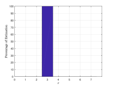
(a) $H_{\text{I},0}$

(b) $H_{\text{I},1}$

(c) $H_{\text{I},2}$, $K_{\text{I},1}=10$

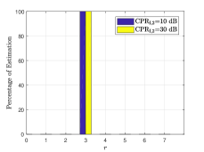
(d) $H_{\text{I},2}$, $K_{\text{I},1}=25$

(e) $H_{\text{I},3}$, $\alpha=1$, $K_{\text{I},2}=4$, $K_{\text{I},3}=20$

(f) $H_{\text{I},3}$, $\alpha=0.1$, $K_{\text{I},2}=10$, $K_{\text{I},3}=25$

Figure 5: Rank estimation performance under $H_{\text{I},l}$, CNR=30 dB

Next, we investigate the behavior of the cyclic procedures for the purposes of $\tau$s estimations in terms of the iteration number $n$. To this end, Fig. 6 shows the average residual errors of

$$\Delta\Psi(n)=\left|\frac{\left[\Psi({\mbox{\boldmath$Z$}}_{S}|\widehat{\bm{\theta}}^{(n)}_{1})-\Psi({\mbox{\boldmath$Z$}}_{S}|\widehat{\bm{\theta}}^{(n-1)}_{1})\right]}{\Psi({\mbox{\boldmath$Z$}}_{S}|\widehat{\bm{\theta}}^{(n)}_{1})}\right|$$ (60)

over 1000 trials against $n$, where $\Psi({\mbox{\boldmath$Z$}}_{S}|\widehat{\bm{\theta}}^{(n)}_{1})$ is the objective function in (20) with the results of $n$th iteration plugged in. It can be observed that, for the considered parameters, the variation is lower than $10^{-4}$ when $n=6$. Similar results can be found under the other hypotheses and not reported here for brevity. As a consequence, we set $n_{\text{max}}=6$ in what follows.

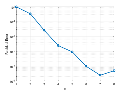
Figure 6: Residual errors versus iteration numbers of the heuristic approach

Table I contains the classification results of 1000 trials when data are generated under $H_{\text{I},0}$. Inspection of the Table highlights that the classification procedure correctly decides $H_{\text{I},0}$ with a $P_{cc}=1$ for all the considered criteria.

TABLE I: Classification results under $H_{\text{I},0}$, CNR=30 dB

	$H_{\text{I},0}$	$H_{\text{I},1}$	$H_{\text{I},2}$	$H_{\text{I},3}$
AIC	1000	0	0	0
GIC2	1000	0	0	0
GIC4	1000	0	0	0
BIC	1000	0	0	0

In Fig. 7, we proceed with the performance under $H_{\text{I},1}$ and plot the $P_{cc}$ versus the $\text{CPR}_{\text{I},1}$. It is observed that when $\text{CPR}_{\text{I},1}$ is small, the scenario cannot be correctly classified since the clutter transition between primary data and secondary data is minor. Moreover, the figure shows that all four criteria exhibit similar classification performance and achieve $P_{cc}\geq 0.75$ when $\text{CPR}_{\text{I},1}\geq 15.7$ dB. More specifically, the BIC slightly outperforms the other criteria and AIC has the worst performance.

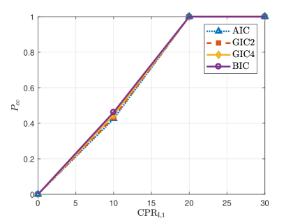
Figure 7: $P_{cc}$ versus $\text{CPR}_{\text{I},1}$ under $H_{\text{I},1}$, CNR=30 dB

Fig. 8 deals with the case where $H_{\text{I},2}$ is true and shows the classification performance with $K_{\text{I},1}=4,10,25$. Under $H_{\text{I},2}$, for all of the illustrated values of $K_{\text{I},1}$, it turns out that AIC exhibits the best performance with remarkable improvement with respect to GIC2, GIC4 and BIC, especially when $K_{\text{I},1}=25$. Further inspections of the figures highlight that the detection capability of the clutter edge at $K_{\text{I},1}=10$ is significantly improved compared with $K_{\text{I},1}=4$, and $K_{\text{I},1}=25$. For example, when $K_{\text{I},1}=10$, the $P_{cc}$ of AIC is greater than 0.75 when $\text{CPR}_{\text{I},2}\geq 9.1$ dB, and this value increases to 15.1 dB and 9.4 dB when $K_{\text{I},1}=4$ and $K_{\text{I},1}=25$, respectively. In other words, the classification architectures are much more sensitive with the power transition located far from the beginning or the end of the reference window. Such result is confirmed by the fact that the clutter edge at $K_{\text{I},1}=4$ exhibits the worst classification performance at least for the considered parameter values.

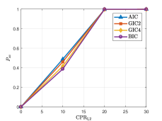
(a) $K_{\text{I},1}=4$

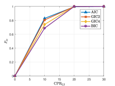
(b) $K_{\text{I},1}=10$

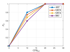
(c) $K_{\text{I},1}=25$

Figure 8: $P_{cc}$ versus $\text{CPR}_{\text{I},2}$ under $H_{\text{I},2}$, CNR=30 dB

In Fig. 9, we plot the $P_{cc}$ under $H_{\text{I},3}$ against $\text{CPR}_{\text{I},3}$ for different clutter edge positions and two different values of $\alpha$, namely $\alpha=1$ and $\alpha=0.1$. It can be seen that under all of the situations of Fig. 9, the AIC ensures the best performance and GIC rules are better than BIC, which confirms what observed in Fig. 8. The figures also show that the classification architectures identify $H_{\text{I},3}$ when $\alpha=1$ much more effectively than when $\alpha=0.1$. For example, when $K_{\text{I},2}=4$, $K_{\text{I},3}=20$, $P_{cc}$ of AIC for $\alpha=1$ is 0.57 at $\text{CPR}_{\text{I},3}=10$ dB and can achieve $P_{cc}=1$ when $\text{CPR}_{\text{I},3}$ increases to 20 dB. On the other hand, for $\alpha=0.1$, the $P_{cc}$ is zero at $\text{CPR}_{\text{I},3}=10$ dB and less than 0.9 even when it increases to $\text{CPR}_{\text{I},3}=20$ dB. This is not a surprising result since the former situation contains greater clutter power. Moreover, we can see that for $\alpha=1$, the classification performance increases when $K_{\text{I},3}-K_{\text{I},2}$ decreases, whereas for $\alpha=0.1$, since the clutter region characterized by $\Delta_{3}$ maintains relatively enough power, the classification performance is more impacted by the significance of the region characterized by $\Delta_{4}$, thus when $\alpha=0.1$, the classification performance increases when $K_{\text{I},3}$ decreases.

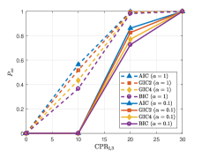
(a) $K_{\text{I},2}=4$, $K_{\text{I},3}=20$

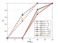
(b) $K_{\text{I},2}=10$, $K_{\text{I},3}=22$

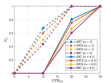
(c) $K_{\text{I},2}=12$, $K_{\text{I},3}=25$

Figure 9: $P_{cc}$ versus $\text{CPR}_{\text{I},3}$ under $H_{\text{I},3}$, CNR=30 dB

The final analysis in this subsection focuses on the estimation capabilities of the proposed approach for what concerns the position of the clutter edge. It is clear that this estimate depends on the extent of power transition between the consecutive homogeneous regions and the size of the reference window. In addition, the edge indices $K_{1}$, $K_{2}$ and $K_{3}$ are generated as discrete uniform random variables taking on values in $K_{\text{I},1}\in\left\{r,\ldots,K_{S}-r\right\}$, $K_{\text{I},2}\in\left\{r,\ldots,\frac{K_{S}}{2}\right\}$, and $K_{\text{I},3}\in\left\{\frac{K_{S}}{2}+1,\ldots,K_{S}-r\right\}$, respectively. In Fig. 10(a), we plot the RMS estimation errors assuming $K_{S}=16,32$, where the estimates of the RMS errors for $K_{\text{I},i},i=1,\ldots,3$ are defined as

$$\text{RMS}_{\text{I},i}=\sqrt{\frac{1}{L}\sum\limits_{l=1}^{L}|\widehat{K}^{(l)}_{\text{I},i}-K_{\text{I},i}|^{2}},$$ (61)

with $\widehat{K}^{(l)}_{\text{I},i}$ the estimate of $K_{\text{I},i}$ at the $l$th trial. The figures highlight that for low CPR values, the error is greater for the configurations associated with larger $K_{S}$, but the curves related to larger $K_{S}$ drop with faster rates than the curves obtained for smaller $K_{S}$. Observe that for CPR values greater than 20 dB, the proposed architecture can return RMS${}_{\text{I},1}$ values less than 2 and RMS${}_{\text{I},l}$, $l=2,3$, values less than 1. Under $H_{\text{I},3}$, the case such that $\alpha\neq 1$ returns similar results except for the larger RMS estimation error values occurring in the presence of low-power clutter regions, and not reported here for brevity.

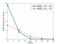
(a) $\text{RMS}_{\text{I},1}$ versus $\text{CPR}_{\text{I},2}$

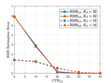
(b) $\text{RMS}_{\text{I},2}$ and $\text{RMS}_{\text{I},3}$ versus $\text{CPR}_{\text{I},3}$, $\alpha=1$

Figure 10: RMS estimation errors, CNR=30 dB

IV-B Clutter Covariance Variation Model 2

The classification and estimation performance of architecture (10) for the more general model of clutter covariance variation is assessed in this subsection. It is of primary importance to underline that when the covariance matrices of each clutter region are totally different, for example, when the angular sectors contributing to the clutter component are not the same (even though maintaining $r$), the proposed architecture returns excellent classification performance (such results are not reported here for brevity). Thus, we assume for simplicity that ${\mbox{\boldmath$R$}}_{l}=\sigma_{c,l}^{2}\sum_{\theta_{i}\in\Theta}{\mbox{\boldmath$v$}}(\theta_{i}){\mbox{\boldmath$v$}}(\theta_{i})^{\dagger}$, $l=1,\ldots,6$, where $\sigma_{c,l}^{2}$ is the clutter power of the $l$th region and ${\mbox{\boldmath$v$}}(\theta_{i})$ is given by (59). Furthermore, $\sigma_{c,l}^{2}$, $l=1,2,3,5$ are computed according to

$$\begin{cases}\text{CPR}_{\text{II},l}=10\log_{10}(\sigma_{c,l}^{2}/\sigma_{c}^{2}),\ l=1,2,3,\\ \text{CPR}_{\text{II},4}=10\log_{10}(\sigma_{c,5}^{2}/\sigma_{c}^{2}),\end{cases}$$ (62)

where $\sigma_{c}^{2}$ is the clutter power of primary data, CPR${}_{\text{II},i}$, $i=1,\ldots,4$ is the CPR value under $H_{\text{II},i}$, $i=1,\ldots,4$. As for $\sigma_{c,4}^{2}$ and $\sigma_{c,6}^{2}$, we define $\sigma_{c,4}^{2}=\beta\sigma_{c,3}^{2}$ with $\beta>0$ a scaling factor, and $\sigma_{c,6}^{2}=1.5\sigma_{c,5}^{2}$.

In Fig. 11, we show the rank estimation performance of BIC rule under $H_{\text{II},i}$, $i=1,\ldots,4$. As for $H_{\text{II},0}$, it is shown in Fig. 5(a). Since correct rank estimation can be ensured as shown in the figures (at least for the illustrated configurations), in what follows we assume that $r$ is known.

(a) $H_{\text{II},1}$

(b) $H_{\text{II},2}$, $K_{\text{II},1}=4$

(c) $H_{\text{II},3}$, $\beta=1$, $K_{\text{II},2}=12$, $K_{\text{II},3}=25$

(d) $H_{\text{II},4}$, $K_{\text{II},4}=10$

Figure 11: Rank estimation performance under $H_{\text{II},i}$, CNR=30 dB

Let us start with assuming that $H_{\text{II},0}$ is in force. Table II contains the specific classification results of the AIC rule for this hypothesis. Inspection of the table highlights that the proposed architecture correctly decides for $H_{\text{II},0}$ with a percentage greater than 0.98.

TABLE II: Classification results under $H_{\text{II},0}$, CNR=30 dB

	$H_{\text{II},0}$	$H_{\text{II},1}$	$H_{\text{II},2}$	$H_{\text{II},3}$	$H_{\text{II},4}$
AIC	983	1	15	1	0
GIC2	1000	0	0	0	0
GIC4	1000	0	0	0	0
BIC	1000	0	0	0	0

For $H_{\text{II},i}$, $i=1,\ldots,4$, results not reported here for brevity indicate that in this case, the AIC criterion overwhelmingly outperforms GIC and BIC. For the specific case, this behavior can be explained by the fact that AIC has the lowest penalty term which decreases the inclination to underfit. For this reason, in what follows, only the performance of AIC are shown. In Fig. 12, we plot the $P_{cc}$ when $H_{\text{II},1}$ is true against $\text{CPR}_{\text{II},1}$. It can be seen that $H_{\text{II},1}$ is correctly identified by the proposed classification architecture with $P_{cc}$ greater than 0.75 when $\text{CPR}_{\text{II},1}\geq 8.3$ dB, and this correct classification probability increases to 0.9 when $\text{CPR}_{\text{II},1}\geq 10$ dB. Fig. 13 deals with the case that $H_{\text{II},2}$ is in force and shows the resulting $P_{cc}$ curves versus $\text{CPR}_{\text{II},2}$ under different values of $K_{\text{II},1}$. As can be observed, in this case, the identification ability of one clutter edge of the proposed architecture is somehow robust with respect to the position of clutter transition and can ensure $P_{cc}>0.75$ when $\text{CPR}_{\text{II},2}\geq 7.85$ dB for all three illustrated configurations.

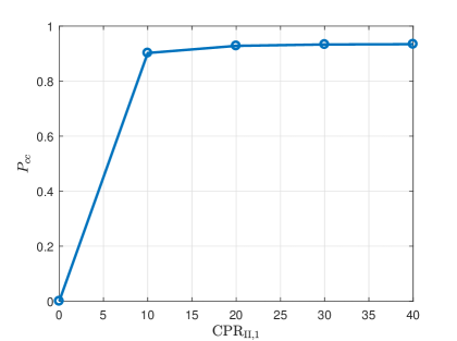
Figure 12: $P_{cc}$ versus $\text{CPR}_{\text{II},1}$ under $H_{\text{II},1}$, CNR=30 dB

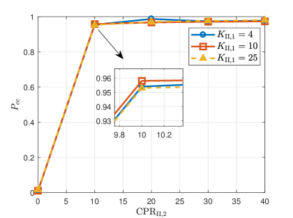
Figure 13: $P_{cc}$ versus $\text{CPR}_{\text{II},2}$ under $H_{\text{II},2}$, CNR=30 dB

In Fig. LABEL:MOS-HII3, we plot the classification performance against $\text{CPR}_{\text{II},3}$ under $H_{\text{II},3}$ with different positions of clutter edges for $\beta=1$ and $\beta=0.5$ in Fig. LABEL:MOS-HII3-beta1 and Fig. LABEL:MOS-HII3-beta05, respectively. It turns out that, as observed under $H_{\text{II},2}$, the classification architecture exhibits similar performance for the three illustrated clutter edge positions. More specifically, $H_{\text{II},3}$ can be correctly identified with $P_{cc}>0.75$ when $\text{CPR}_{\text{II},3}$ greater than 8.2 dB and 16.7 dB for $\beta=1$ and $\beta=0.5$, respectively. Further inspections of the two figures highlight that $P_{cc}$ for $\beta=0.5$ significantly decreases compared with that for $\beta=1$ due to the lower power of the clutter region characterized by smaller $\sigma_{c,4}^{2}$. Fig. LABEL:MOS-HII4 shows that the proposed classification architecture can correctly classify $H_{\text{II},4}$ with $P_{cc}>0.75$ at $\text{CPR}_{\text{II},4}$ greater than 18.4 dB.

Furthermore, to depict a more complete picture of the classification capabilities, Fig. 14 contains the specific results under $H_{\text{II},3}$ with $\text{CPR}_{\text{II},3}=10$ dB, $\beta=0.5$, and $H_{\text{II},4}$ with $\text{CPR}_{\text{II},4}=10$ dB, respectively. The figures show that for relatively low $\text{CPR}_{\text{II},3}$, $H_{\text{II},3}$ is mainly misidentified as $H_{\text{II},2}$ when $\beta\neq 1$, whereas for the cases that $\text{CPR}_{\text{II},4}$ is not large, $H_{\text{II},4}$ is inclined to be misclassified as $H_{\text{II},1}$ since the extent of clutter transition within the secondary data is less significant when $\sigma_{c,6}^{2}=1.5\sigma_{c,5}^{2}$.

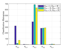
(a) $H_{\text{II},3}$, $\text{CPR}_{\text{II},3}=10$ dB, $\beta=0.5$

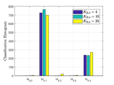
(b) $H_{\text{II},4}$, $\text{CPR}_{\text{II},4}=10$ dB

Figure 14: Classification results under $H_{\text{II},3}$ and $H_{\text{II},4}$, CNR=30 dB

The final analysis concerns the estimation capability of the clutter edge positions in terms of the RMS estimation errors of $K_{\text{II},i},i=1,\ldots,4$, defined as

$$\text{RMS}_{\text{II},i}=\sqrt{\frac{1}{L}\sum\limits_{l=1}^{L}|\widehat{K}^{(l)}_{\text{II},i}-K_{\text{II},i}|^{2}},$$ (63)

with $\widehat{K}^{(l)}_{\text{II},i}$ the estimate of $K_{\text{II},i}$ at the $l$th trial. The results are shown in Fig. 15 for different values of parameters. In Fig. 15, the edge indices are generated as discrete uniform random variables taking on values in $K_{\text{II},1}\in\left\{r,\ldots,K_{S}-r\right\}$, $K_{\text{II},2}\in\left\{r,\ldots,\frac{K_{S}}{2}\right\}$, $K_{\text{II},3}\in\left\{\frac{K_{S}}{2}+1,\ldots,K_{S}-r\right\}$, and $K_{\text{II},4}\in\left\{r,\ldots,K_{S}-r\right\}$ respectively. From the figures, what has been shown in Fig. 10 is confirmed that at low CPR values, the estimation procedure associated smaller $K_{S}$ exhibits lower RMS estimation errors.

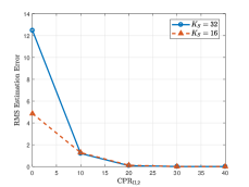
(a) $\text{RMS}_{\text{II},1}$ versus $\text{CPR}_{\text{II},2}$

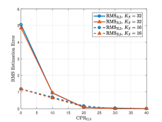
(b) $\text{RMS}_{\text{II},2}$ and $\text{RMS}_{\text{II},3}$ versus $\text{CPR}_{\text{II},3}$, $\beta=1$

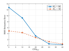
(c) $\text{RMS}_{\text{II},4}$ versus $\text{CPR}_{\text{II},4}$

Figure 15: RMS estimation errors, CNR=30 dB

V Conclusion

In this paper, we have provided a solution to the problem of classifying the radar operating scenario in terms of clutter statistical properties within the radar reference window. The newly conceived architectures are also capable of effectively estimating the clutter rank. Unlike existing classifiers, at the design stage we have considered two models for the clutter variation over the range and several configurations, including the traditional homogeneous environment, a new formulation of the partially-homogeneous environment, as well as the cases where one or two clutter edges are present. The classification problems have been formulated in terms of multiple hypothesis testing problems and solved by means of suitable approximations of the MOS rules due to the intractable mathematics associated with maximum likelihood estimation of some unknown parameters. The performance analysis conducted on simulated data has confirmed the effectiveness of the proposed architectures in deciding for the correct operating scenario (hypothesis). More importantly, the classification results provided by the proposed algorithms represent clutter maps that allow the system to select the most adequate set of secondary data for the current scenario and, hence, to improve the detection performance.

Future research tracks may include the extension of this work to the case where clutter discretes are included in the region of interest or the design of joint classification and detection architectures. Another related issue may concern the design of classification architectures that exploit possible knowledge about the background and/or systems leading to specific clutter covariance structures and, at the same time, more reliable parameter estimation performances.

Appendix A Estimation of $U$in (14)

In this appendix, we describe the optimization criterion leading to the estimate of $\bm{U}$ under $H_{\text{I},1}$. To this end, notice that the optimization problem with respect to $\bm{U}$ is tantamount to

$$\max\limits_{\bm{U}} -\sum_{k=1}^{K_{P}}{\mbox{\boldmath$z$}}_{k}^{\dagger}\bm{U}(\sigma^{2}{\mbox{\boldmath$I$}}+\bm{\Lambda})^{-1}\bm{U}^{\dagger}{\mbox{\boldmath$z$}}_{k}$$

$$\qquad-\sum_{k=1}^{K_{S}}{\mbox{\boldmath$r$}}_{k}^{\dagger}\bm{U}(\sigma^{2}{\mbox{\boldmath$I$}}+\bm{\Gamma}_{1}\bm{\Lambda}\bm{\Gamma}_{1})^{-1}\bm{U}^{\dagger}{\mbox{\boldmath$r$}}_{k}$$

$$\Rightarrow \max\limits_{\bm{U}} -\sum_{k=1}^{K_{P}}||{\mbox{\boldmath$z$}}_{k}||^{2}\bm{\alpha}_{k}^{\dagger}\bm{U}(\sigma^{2}{\mbox{\boldmath$I$}}+\bm{\Lambda})^{-1}\bm{U}^{\dagger}\bm{\alpha}_{k}$$

$$\qquad-\sum_{k=1}^{K_{S}}||{\mbox{\boldmath$r$}}_{k}||^{2}\bm{\beta}_{k}^{\dagger}\bm{U}(\sigma^{2}{\mbox{\boldmath$I$}}+\bm{\Gamma}_{1}\bm{\Lambda}\bm{\Gamma}_{1})^{-1}\bm{U}^{\dagger}\bm{\beta}_{k}$$

$$\Rightarrow \max\limits_{\bm{U}} -\sum_{k=1}^{K_{P}+K_{S}}\bm{\xi}_{k}^{\dagger}\bm{U}(\sigma^{2}{\mbox{\boldmath$I$}}+{\mbox{\boldmath$Q$}}_{1,k}\bm{\Lambda}{\mbox{\boldmath$Q$}}_{1,k})^{-1}\bm{U}^{\dagger}\bm{\xi}_{k}\cdot b_{k}$$

$$\Rightarrow \min\limits_{\bm{U}} \sum_{k=1}^{K_{P}+K_{S}}\bm{\xi}_{k}^{\dagger}\bm{U}{\mbox{\boldmath$D$}}_{1,k}\bm{U}^{\dagger}\bm{\xi}_{k},$$ (64)

where $\bm{\alpha}_{k}={\mbox{\boldmath$z$}}_{k}/||{\mbox{\boldmath$z$}}_{k}||$, $k=1,\ldots,K_{P}$, $\bm{\beta}_{k}={\mbox{\boldmath$r$}}_{k}/||{\mbox{\boldmath$r$}}_{k}||$, $k=1,\ldots,K_{S}$,

$$\bm{\xi}_{k}=\left\{\begin{array}[]{lll}\bm{\alpha}_{k},&\ k=1,\ldots,K_{P},\\ \bm{\beta}_{k-K_{P}},&\ k=K_{P}+1,\ldots,K_{P}+K_{S},\end{array}\right.$$ (67)

and ${\mbox{\boldmath$D$}}_{1,k}=b_{k}(\sigma^{2}{\mbox{\boldmath$I$}}+{\mbox{\boldmath$Q$}}_{1,k}\bm{\Lambda}{\mbox{\boldmath$Q$}}_{1,k})^{-1}$ with

$$b_{k}=\left\{\begin{array}[]{lll}||{\mbox{\boldmath$z$}}_{k}||^{2},&\ k=1,\ldots,K_{P},\\ ||{\mbox{\boldmath$r$}}_{k-K_{P}}||^{2},&\ k=K_{P}+1,\ldots,K_{P}+K_{S},\end{array}\right.$$ (70)

$${\mbox{\boldmath$Q$}}_{1,k}=\left\{\begin{array}[]{lll}{\mbox{\boldmath$I$}},&\ \ \ k=1,\ldots,K_{P},\\ \bm{\Gamma}_{1},&\ \ \ k=K_{P}+1,\ldots,K_{P}+K_{S}.\end{array}\right.$$ (73)

Now, let us observe that for all ${k=1,\ldots,K_{P}+K_{S}}$ the minimum eigenvalue of ${\mbox{\boldmath$D$}}_{1,k}$ is $\delta_{1,k}=\frac{b_{k}}{\sigma^{2}+q_{1,k}\lambda_{1}}$ and the corresponding eigenvector is $\bm{e}_{1}=[1,0,\ldots,0]^{T}$, where $q_{1,k}$ is the square of ${\mbox{\boldmath$Q$}}_{1,k}(1,1)$. Therefore, for a given $k\in\left\{1,\ldots,K_{P}+K_{S}\right\}$, by the Rayleigh-Ritz Theorem [70], the unitary matrix $\bm{U}$ satisfying $\bm{U}^{\dagger}\bm{\xi}_{k}=\bm{e}_{1}$ minimizes $\bm{\xi}_{k}^{\dagger}\bm{U}{\mbox{\boldmath$D$}}_{1,k}\bm{U}^{\dagger}\bm{\xi}_{k}$, and the minimum is $\delta_{1,k}$. However, it is not possible to obtain a $\bm{U}$ such that $\bm{U}^{\dagger}\bm{\xi}_{k}=\bm{e}_{1}$, $\forall{k}\in\left\{1,\ldots,K_{P}+K_{S}\right\}$. For this reason, we resort to a suboptimum approach which consists in minimizing the norm of the residual error between $\bm{U}^{\dagger}\bm{\xi}_{k}$ and $\bm{e}_{1}$ for all $k=1,\ldots,K_{P}+K_{S}$. Specifically, we estimate $\bm{U}$ by solving

$$\min\limits_{\bm{U}\atop{\bm{U}^{\dagger}\bm{U}=\bm{U}\bm{U}^{\dagger}=\bm{I}}}\sum\limits_{k=1}^{K_{P}+K_{S}}||\bm{U}^{\dagger}\bm{\xi}_{k}-\bm{e}_{1}||^{2},$$ (74)

The above problem can be written as

$$\min\limits_{\bm{U}\atop{\bm{U}^{\dagger}\bm{U}=\bm{U}\bm{U}^{\dagger}=\bm{I}}} \sum_{k=1}^{K_{P}+K_{S}}\left[\bm{\xi}_{k}^{\dagger}\bm{U}\bm{U}^{\dagger}\bm{\xi}_{k}-\bm{\xi}_{k}^{\dagger}\bm{U}\bm{e}_{1}\right.$$

$$\left.-\bm{e}_{1}^{\dagger}\bm{U}^{\dagger}\bm{\xi}_{k}+\bm{e}_{1}^{\dagger}\bm{e}_{1}\right]$$

$$\Rightarrow \min\limits_{\bm{U}\atop{\bm{U}^{\dagger}\bm{U}=\bm{U}\bm{U}^{\dagger}=\bm{I}}} \sum_{k=1}^{K_{P}+K_{S}}\left[2-\bm{\xi}_{k}^{\dagger}\bm{U}\bm{e}_{1}-\bm{e}_{1}^{\dagger}\bm{U}^{\dagger}\bm{\xi}_{k}\right]$$

$$\Rightarrow \min\limits_{\bm{d}:||\bm{d}||^{2}=1} \left[2-\bm{\mu}^{\dagger}\bm{d}-\bm{d}^{\dagger}\bm{\mu}\right]$$

$$\Rightarrow \min\limits_{\bm{d}:||\bm{d}||^{2}=1} \left[||\bm{d}-\bm{\mu}||^{2}+C\right],$$ (75)

where $\bm{d}=\bm{U}\bm{e}_{1}$, $\bm{\mu}=\sum_{k=1}^{K_{P}+K_{S}}\bm{\xi}_{k}$ and $C$ is a constant. The last problem can be further recast as follows

$$\left\{\begin{array}[]{lll}\min\limits_{\bm{d}}||\bm{d}-\bm{\mu}||^{2},\\ \text{subject \ to}\ ||\bm{d}||^{2}=1.\end{array}\right.$$ (76)

Using the Lagrange multipliers method, the Lagrangian is given by

$$L(\bm{d},\lambda)=||\bm{d}-\bm{\mu}||^{2}-\lambda(||\bm{d}||^{2}-1)$$ (77)

and setting to zero the first derivative of (77) with respect to $\bm{d}$ and $\lambda$, we come up with

$$\left\{\begin{array}[]{lll}\widehat{\lambda}=1-||\bm{\mu}||,\\ \widehat{\bm{d}}=\frac{\bm{\mu}}{||\bm{\mu}||}.\end{array}\right.$$ (78)

It follows that $\bm{U}$ is any unitary matrix which rotates $\bm{e}_{1}$ to $\widehat{\bm{d}}$ and is given, for instance, by resorting to the singular value decomposition of $\widehat{\bm{d}}$. Notice that such a choice ensures that for all $k=1,\ldots,K_{P}+K_{S}$, the first component of $\bm{\xi}_{k}$ is greater than the remaining.

Chaoran Yin received the B.S. degree in electromagnetic fields and wireless technology from Northwestern Polytechnical University, Xi’an, Shaanxi, China, in 2018. He is currently working toward the Ph.D. degree in signal and information processing with Institute of Acoustics, Chinese Academy of Sciences, and University of Chinese Academy of Sciences, Beijing, China.

Linjie Yan received the B.E. degree in communication engineering from Shandong University of Science and Technology, and the Ph.D. degree in signal and information processing from the Institute of Acoustics, Chinese Academy of Sciences, Beijing, China, in 2016 and 2021, respectively. She is currently a Post-doctor with the Institute of Acoustics, Chinese Academy of Sciences, Beijing, China. Her research interests include statistical signal processing with more emphasis on adaptive sonar and radar signal processing.

Chengpeng Hao (Senior Member, IEEE) received the B.S. and M.S. degrees in electronic engineering from Beijing Broadcasting Institute, Beijing, China, in 1998 and 2001, respectively, and the Ph.D. degree in signal and information processing from the Institute of Acoustics, Chinese Academy of Sciences, Beijing (IACAS), China, in 2004. He is currently a full professor with IACAS. He has held a visiting position with the Electrical and Computer Engineering Department, Queens University, Kingston, ON, Canada, from July 2013 to July 2014. He has authored or coauthored more than 160 journal and conference papers. His research interests are in the fields of statistical signal processing and array signal processing. Dr. Hao is currently serving as an Associate Editor for several international journals, including IEEE ACCESS, Signal, Image and Video Processing (Springer), and the Journal of Engineering (IET).

Silvia Liberata Ullo (Senior Member, IEEE) received the degree (cum laude) in electronic engineering from the Faculty of Engineering, Federico II University, Naples, Italy, in 1989, and the M.Sc. degree from the Sloan Business School of Boston, Massachusetts Institute of Technology (MIT), Cambridge, MA, USA, in June 1992. She is an Industry Liaison for the IEEE Joint ComSoc/Vehicular Technology Membership (VTS) Italy Chapter. She was the National Referent for International Federation of Business and Professional Women (FIDAPA BPW) Italy Science and Technology Task Force from 2019 to 2021. She has been a researcher with the Department of Engineering, University of Sannio, Benevento, Italy, since 2004. She is a Member of the Academic Senate and the Ph.D. Professors Board. She is teaching signal theory and elaboration, and telecommunication networks for electronic engineering, and optical and radar remote sensing for the Ph.D. course. She has authored 80+ research articles, coauthored many book chapters and served as the Editor of two books, and many special issues in reputed journals of her research sectors. Her main interests include signal processing, remote sensing, satellite data analysis, machine learning and quantum ML, radar systems, sensor networks, and smart grids. She has worked in the private and public sector from 1992 to 2004, before joining the University of Sannio.

Gaetano Giunta (Senior Member, IEEE) received the M.S. degree electronic engineering from the University of Pisa, Pisa, Italy and the Ph.D. degree in information and communication engineering from the University of Rome La Sapienza, Rome, Italy, in 1985 and 1990, respectively. During 1989-1990, he was also a Research Fellow with Signal Processing Laboratory, the École Polytechnique Fédérale de Lausanne, Lausanne, Switzerland. In 1992, he became an Assistant Professor with the INFO-COM Department, University of Rome La Sapienza. In 1998, he taught signal processing with the University of Roma Tre, Rome, Italy. From 2001 to 2005, he was with the University of Roma Tre as an Associate Professor of telecommunications. Since 2005, he has been a Full Professor of telecommunications with the same University. His main research interests include signal and image processing for mobile communications and wireless networks. He is a Member of the IEEE Societies of Communications, Signal Processing, and Vehicular Technology. He was also a Reviewer for various IEEE Transactions, IET (formerly IEE) proceedings, and EURASIP journals, and a TPC Member for various international conferences and symposia in the same fields.

Alfonso Farina (Life Fellow, IEEE) received the Doctoral Laurea - degree in electronic engineering from the University of Rome, Rome, Italy, in 1973. In 1974, he joined SELENIA S.P.A., then Selex ES, where he became the Director of the Analysis of Integrated Systems Unit, and the Director of Engineering of the Large Business Systems Division. In 2012, he was the Senior VP and the Chief Technology Officer (CTO) of the Company, reporting directly to the President. From 2013 to 2014, he was a Senior Advisor to the CTO. He retired in October 2014. From 1979 to 1985, he was also a Professor of radar techniques with the University of Naples, Naples, Italy. He is currently a Visiting Professor with the Department of Electronic and Electrical Engineering, University College London, London, U.K., and with the Centre of Electronic Warfare, Information and Cyber, Cranfield University, Cranfield, U.K., a Distinguished Lecturer of the IEEE Aerospace and Electronic Systems Society and a Distinguished Industry Lecturer for the IEEE Signal Processing Society during January 2018-December 2019. He is a Consultant to Leonardo S.p.A. Land and Naval Defence Electronics Division, Rome. He has authored or coauthored more than 800 peer-reviewed technical papers and books and monographs (published worldwide), some of them also translated in to Russian and Chinese. Dr. Farina has been an IEEE Signal Processing Magazine Senior Editorial Board Member (three-year term) since 2017. He was the Conference General Chairman of the IEEE Radar Con 2008, Rome, Italy, May 2008, and the Executive Conference Chair at the International Conference on Information Fusion, Florence, Italy, July 2006. He is the Honorary Chair of IEEE Radar Conf September 2020, Florence. He was the recipient of many awards, including Leader of the team that won the First Prize of the first edition of the Finmeccanica Award for Innovation Technology, out of more than 330 submitted projects by the Companies of Finmeccanica Group in 2004, an International Fellow of the Royal Academy of Engineering, U.K. in 2005, the fellowship was presented to him by HRH Prince Philip, the Duke of Edinburgh, IEEE Dennis J. Picard Medal for Radar Technologies and Applications for Continuous, Innovative, Theoretical, and Practical Contributions to Radar Systems and Adaptive Signal Processing Techniques in 2010, IEEE Honor Ceremony, Montreal, Canada, Oscar Masi Award for the AULOS green radar by the Italian Industrial Research Association (AIRI) in 2012, IET Achievement Medal for Outstanding contributions to radar system design, signal, data and image processing, and data fusion in 2014, IEEE SPS Industrial Leader Award for contributions to radar array processing and industrial leadership in 2017, 2019 Christian Hulsmeyer Award from the German Institute of Navigation (DGON), with the motivation: In appreciation of his outstanding contribution to radar research and education. He was the recipient of Best Paper Awards, such as the B. Carlton of IEEE TRANSACTIONS ON AEROSPACE AND ELECTRONIC SYSTEMS in 2001, 2003, and 2013, IET-Proceeding on Radar Sonar and Navigation during 2009-2010, and International Conference on Information Fusion in 2004. In the past few decades, he has been collaborating with several professional journals and conferences (mainly on radar and data fusion) as an Associate Editor, Reviewer, organizer of special issues, Session Chairman, and Plenary Speaker. He is a Fellow of the IET, a Fellow of the Royal Academy of Engineering, and a Fellow of EURASIP. Since 2017, he has been the Chair of Italy Section Chapter, IEEE AESS-10, and a Member of the IEEE AESS BoG, Jan 2019-Dec 2021. In 26 October 2018, he was interviewed, among few top managers of the Company, at RAI Storia for the 70th anniversario di Leonardo Company (70th anniversary of Leonardo Company). Since 2010, he has also been a Fellow of EURASIP. Starting from 2020, he is a Member of European Academy of Science.

Danilo Orlando (Senior Member, IEEE) was born in Gagliano del Capo, Italy, in August 1978. He received the Dr. Eng. degree (Hons.) in computer engineering and the Ph.D. degree (Hons.) in information engineering from the University of Salento (formerly University of Lecce), Lecce, Italy, in 2004 and 2008, respectively. From July 2007 to July 2010, he was with the University of Cassino, Cassino, Italy, engaged in a research project on algorithms for track-before-detect of multiple targets in uncertain scenarios. From September to November 2009, he was a Visiting Scientist with the NATO Undersea Research Centre, La Spezia, Italy. From September 2011 to April 2015, he was with Elettronica S.p.A. engaged as a System Analyst in the field of electronic warfare. In May 2015, he joined the Università degli Studi Niccolò Cusano, Rome, Italy, where he is currently an Associate Professor. In 2007, he has held visiting positions with the Department of Avionics and Systems, ENSICA (now Institut Supérieur de l’Aéronautique et de l’Espace, ISAE), Toulouse, France, and from 2017 to 2019, he was with the Chinese Academy of Science, Beijing, China. He is the author or coauthor of more than 150 scientific publications in international journals, conferences, and books. His main research interests include statistical signal processing with more emphasis on adaptive detection and tracking of multiple targets in multisensor scenarios. He was a Senior Area Editor of the IEEE TRANSACTIONS ON SIGNAL PROCESSING. He is currently an Associate Editor for the IEEE OPEN JOURNAL ON SIGNAL PROCESSING, EURASIP Journal on Advances in Signal Processing, and Remote Sensing (MDPI).

References

- [1] M. A. Richards, W. L. Melvin, J. A. Scheer, and W. A. Holm, Principles of Modern Radar: Radar Applications, Volume 3, ser. Electromagnetics and Radar. Institution of Engineering and Technology, 2013.
- [2] C. Hao, D. Orlando, J. Liu, and C. Yin, Advances in Adaptive Radar Detection and Range Estimation, Springer, Ed., Singapore, 2022.
- [3] A. Farina, “Electronic counter-countermeasures,” in Radar Handbook, 3rd ed. McGraw-Hill, 2008, ch. 24.
- [4] E. J. Kelly, “An adaptive detection algorithm,” IEEE Transactions on Aerospace and Electronic Systems, vol. 22, no. 1, pp. 115–127, 1986.
- [5] F. C. Robey, D. R. Fuhrmann, E. J. Kelly, and R. Nitzberg, “A CFAR adaptive matched filter detector,” IEEE Transactions on Aerospace and Electronic Systems, vol. 28, no. 1, pp. 208–216, 1992.
- [6] E. J. Kelly and K. Forsythe, “Adaptive Detection and Parameter Estimation for Multidimensional Signal Models,” Lincoln Lab, MIT, Lexington, US, Technical Report 848, 1989.
- [7] F. Bandiera, D. Orlando, and G. Ricci, Advanced radar detection schemes under mismatch signal models; synthesis lectures on signal process, M. . C. P. Synthesis Lectures on Signal Processing No. 8, Ed., San Rafael, US, 2009.
- [8] E. Conte, A. De Maio, and G. Ricci, “GLRT-based adaptive detection algorithms for range-spread targets,” IEEE Transactions on Signal Processing, vol. 49, no. 7, pp. 1336–1348, July 2001.
- [9] P. Addabbo, S. Han, F. Biondi, G. Giunta, and D. Orlando, “Adaptive Radar Detection in the Presence of Multiple Alternative Hypotheses Using Kullback-Leibler Information Criterion-Part II: Applications,” IEEE Transactions on Signal Processing, vol. 69, pp. 3742–3754, 2021.
- [10] C. Hao, D. Orlando, G. Foglia, and G. Giunta, “Knowledge-based adaptive detection: Joint exploitation of clutter and system symmetry properties,” IEEE Signal Processing Letters, vol. 23, no. 10, pp. 1489–1493, 2016.
- [11] L. Cai and H. Wang, “A Persymmetric Multiband GLR Algorithm,” IEEE Transactions on Aerospace and Electronic Systems, vol. 28, no. 3, pp. 806–816, 1992.
- [12] J. Zheng, R. Chen, T. Yang, X. Liu, H. Liu, T. Su, and L. Wan, “An Efficient Strategy for Accurate Detection and Localization of UAV Swarms,” IEEE Internet of Things Journal, vol. 8, no. 20, pp. 15 372–15 381, 2021.
- [13] S. Yan, D. Massaro, D. Orlando, C. Hao, and A. Farina, “Adaptive detection and range estimation of point-like targets with symmetric spectrum,” IEEE Signal Processing Letters, vol. 24, no. 11, pp. 1744–1748, 2017.
- [14] F. Bandiera, O. Besson, D. Orlando, G. Ricci, and L. L. Scharf, “GLRT-Based Direction Detectors in Homogeneous Noise and Subspace Interference,” IEEE Transactions on Signal Processing, vol. 55, no. 6, pp. 2386–2394, June 2007.
- [15] K. Gerlach and M. Steiner, “Adaptive detection of range distributed targets,” IEEE Transactions on Signal Processing, vol. 47, no. 7, pp. 1844–1851, 1999.
- [16] A. Aubry, A. De Maio, G. Foglia, C. Hao, and D. Orlando, “Radar detection and range estimation using oversampled data,” IEEE Transactions on Aerospace and Electronic Systems, vol. 51, no. 2, pp. 1039–1052, 2015.
- [17] K. Gerlach, M. Steiner, and F. Lin, “Detection of a spatially distributed target in white noise,” IEEE Signal Processing Letters, vol. 4, no. 7, pp. 198–200, 1997.
- [18] F. Bandiera, D. Orlando, and G. Ricci, “CFAR detection of extended and multiple point-like targets without assignment of secondary data,” IEEE Signal Processing Letters, vol. 13, no. 4, pp. 240–243, 2006.
- [19] L. L. Scharf and B. Friedlander, “Matched subspace detectors,” IEEE Transactions on Signal Processing, vol. 42, no. 8, pp. 2146–2157, Aug 1994.
- [20] F. Bandiera, A. D. Maio, A. S. Greco, and G. Ricci, “Adaptive Radar Detection of Distributed Targets in Homogeneous and Partially Homogeneous Noise Plus Subspace Interference,” IEEE Transactions on Signal Processing, vol. 55, no. 4, pp. 1223–1237, April 2007.
- [21] J. Zheng, T. Yang, H. Liu, T. Su, and L. Wan, “Accurate Detection and Localization of Unmanned Aerial Vehicle Swarms-Enabled Mobile Edge Computing System,” IEEE Transactions on Industrial Informatics, vol. 17, no. 7, pp. 5059–5067, 2021.
- [22] A. De Maio, D. Orlando, C. Hao, and G. Foglia, “Adaptive Detection of Point-like Targets in Spectrally Symmetric Interference,” IEEE Transactions on Signal Processing, vol. 64, no. 12, pp. 3207–3220, June 2016.
- [23] W. Liu, J. Liu, C. Hao, Y. Gao, and Y. Wang, “Multichannel adaptive signal detection: Basic theory and literature review,” Science China Information Sciences, vol. 65, no. 121301, 2022.
- [24] C. Hao, S. Gazor, X. Ma, S. Yan, C. Hou, and D. Orlando, “Polarimetric Detection and Range Estimation of a Point-Like Target,” IEEE Transactions on Aerospace and Electronic Systems, vol. 52, no. 2, pp. 603–616, April 2016.
- [25] C. Hao, S. Gazor, G. Foglia, B. Liu, and C. Hou, “Persymmetric adaptive detection and range estimation of a small target,” IEEE Transactions on Aerospace and Electronic Systems, vol. 51, no. 4, pp. 2590–2604, October 2015.
- [26] D. Orlando and G. Ricci, “Adaptive Radar Detection and Localization of a Point-Like Target,” IEEE Transactions on Signal Processing, vol. 59, no. 9, pp. 4086–4096, 2011.
- [27] D. Orlando and G. Ricci, “A Rao test with enhanced selectivity properties in homogeneous scenarios,” IEEE Transactions on Signal Processing, vol. 58, no. 10, pp. 5385–5390, October 2010.
- [28] A. De Maio and D. Orlando, “An invariant approach to adaptive radar detection under covariance persymmetry,” IEEE Transactions on Signal Processing, vol. 63, no. 5, pp. 1297–1309, January 2015.
- [29] D. Orlando, G. Ricci, and L. L. Scharf, “A Unified Theory of Adaptive Subspace Detection Part I: Detector Designs,” IEEE Transactions on Signal Processing, vol. 70, pp. 4925–4938, 2022.
- [30] J. Guerci, Cognitive Radar: The Knowledge-aided Fully Adaptive Approach, ser. Artech House radar library. Artech House, 2010.
- [31] J. Guerci, Space-Time Adaptive Processing for Radar, Second Edition, ser. Artech House radar library. Artech House Publishers, 2014.
- [32] S. Kraut and L. L. Scharf, “The CFAR adaptive subspace detector is a scale-invariant GLRT,” IEEE Transactions on Signal Processing, vol. 47, no. 9, pp. 2538–2541, September 1999.
- [33] C. Hao, D. Orlando, G. Foglia, X. Ma, S. Yan, and C. Hou, “Persymmetric adaptive detection of distributed targets in partially-homogeneous environment,” Digital signal processing, vol. 24, no. 1, pp. 42–51, 2014.
- [34] C. Hao, D. Orlando, G. Foglia, X. Ma, and C. Hou, “Adaptive Radar Detection and Range Estimation with Oversampled Data for Partially Homogeneous Environment,” IEEE Signal Processing Letters, vol. 22, no. 9, pp. 1359–1363, 2015.
- [35] L. Yan, C. Hao, D. Orlando, A. Farina, and C. Hou, “Parametric Space-Time Detection and Range Estimation of Point-Like Targets in Partially Homogeneous Environment,” IEEE Transactions on Aerospace and Electronic Systems, vol. 56, no. 2, pp. 1228–1242, 2020.
- [36] G. Foglia, C. Hao, A. Farina, G. Giunta, D. Orlando, and C. Hou, “Adaptive Detection of Point-like Targets in Partially Homogeneous Clutter with Symmetric Spectrum,” IEEE Transactions on Aerospace and Electronic Systems, vol. 53, no. 4, pp. 2110–2119, August 2017.
- [37] C. Hao, D. Orlando, X. Ma, and C. Hou, “Persymmetric Rao and Wald Tests for Partially Homogeneous Environment,” IEEE Signal Processing Letters, vol. 19, no. 9, pp. 587–590, September 2012.
- [38] W. Liu, W. Xie, J. Liu, and Y. Wang, “Adaptive Double Subspace Signal Detection in Gaussian Background-Part II: Partially Homogeneous Environments,” IEEE Transactions on Signal Processing, vol. 62, no. 9, pp. 2358–2369, May 2014.
- [39] C. Hao, D. Orlando, A. Farina, S. Iommelli, and C. Hou, “Symmetric spectrum detection in the presence of partially homogeneous environment,” in IEEE Radar Conference (RadarConf), May 2016, pp. 1–4.
- [40] Y. Gao, G. Liao, S. Zhu, X. Zhang, and D. Yang, “Persymmetric Adaptive Detectors in Homogeneous and Partially Homogeneous Environments,” IEEE Transactions on Signal Processing, vol. 62, no. 2, pp. 331–342, January 2014.
- [41] A. De Maio, C. Hao, and D. Orlando, “An adaptive detector with range estimation capabilities for partially homogeneous environment,” IEEE Signal Processing Letters, vol. 21, no. 3, pp. 325–329, May 2014.
- [42] J. Liu, D. Massaro, D. Orlando, and A. Farina, “Radar Adaptive Detection Architectures for Heterogeneous Environments,” IEEE Transactions on Signal Processing, vol. 68, pp. 4307–4319, 2020.
- [43] E. Conte, A. De Maio, and G. Ricci, “Recursive estimation of the covariance matrix of a compound-Gaussian process and its application to adaptive CFAR detection,” IEEE Transactions on Signal Processing, vol. 50, no. 8, pp. 1908–1915, August 2002.
- [44] S. H. G. Yilmaz, C. Zarro, H. T. Hayvaci, and S. L. Ullo, “Adaptive Waveform Design with Multipath Exploitation Radar in Heterogeneous Environments,” Remote Sensing, vol. 13, no. 9, 2021.
- [45] A. Coluccia, D. Orlando, and G. Ricci, “A GLRT-like CFAR detector for heterogeneous environments,” Signal Processing, vol. 194, p. 108401, 2022.
- [46] S. Haykin and C. Deng, “Classification of radar clutter using neural networks,” IEEE Transactions on Neural Networks, vol. 2, no. 6, pp. 589–600, 1991.
- [47] C. Bouvier, L. Martinet, G. Favier, H. Sedano, and M. Artaud, “Radar clutter classification using autoregressive modelling, K-distribution and neural network,” in 1995 International Conference on Acoustics, Speech, and Signal Processing, vol. 3, 1995, pp. 1820–1823 vol.3.
- [48] L. Zhang, A. Xue, X. Zhao, S. Xu, and K. Mao, “Sea-Land Clutter Classification Based on Graph Spectrum Features,” Remote Sensing, vol. 13, no. 22, 2021. [Online]. Available: https://www.mdpi.com/2072-4292/13/22/4588
- [49] K. P. Murphy, Machine Learning: A Probabilistic Perspective, T. M. Press, Ed., Massachusetts, US, 2012.
- [50] V. Carotenuto, A. De Maio, D. Orlando, and P. Stoica, “Model Order Selection rules for covariance structure classification in radar,” IEEE Transactions on Signal Processing, vol. 65, no. 20, pp. 5305–5317, 2017.
- [51] C. V., A. De Maio, D. Orlando, and P. Stoica, “Radar detection architecture based on interference covariance structure classification,” IEEE Transactions on Aerospace and Electronic Systems, vol. 55, no. 2, pp. 607–618, April 2019.
- [52] P. Stoica and Y. Selen, “Model-order selection: A review of information criterion rules,” IEEE Signal Processing Magazine, vol. 21, no. 4, pp. 36–47, 2004.
- [53] P. Stoica, Y. Selen, and J. Li, “On information criteria and the generalized likelihood ratio test of model order selection,” IEEE Signal Processing Letters, vol. 11, no. 10, pp. 794–797, 2004.
- [54] C. V., D. Orlando, and A. Farina, “Interference Covariance Matrix Structure Classification in Heterogeneous Environment,” IEEE Signal Processing Letters, vol. 26, no. 10, pp. 1491–1495, October 2019.
- [55] J. Liu, F. Biondi, D. Orlando, and A. Farina, “Training Data Classification Algorithms for Radar Applications,” IEEE Signal Processing Letters, vol. 26, no. 10, pp. 1446–1450, October 2019.
- [56] D. Xu, P. Addabbo, C. Hao, J. Liu, D. Orlando, and A. Farina, “Adaptive strategies for clutter edge detection in radar,” Signal Processing, vol. 186, p. 108127, 2021.
- [57] T. Wang, D. Xu, C. Hao, P. Addabbo, and D. Orlando, “Clutter Edges Detection Algorithms for Structured Clutter Covariance Matrices,” IEEE Signal Processing Letters, vol. 29, pp. 642–646, 2022.
- [58] P. Addabbo, S. Han, D. Orlando, and G. Ricci, “Learning Strategies for Radar Clutter Classification,” IEEE Transactions on Signal Processing, vol. 69, pp. 1070–1082, 2021.
- [59] G. Capraro, A. Farina, H. Griffiths, and M. Wicks, “Knowledge-based radar signal and data processing: a tutorial review,” IEEE Signal Processing Magazine, vol. 23, no. 1, pp. 18–29, 2006.
- [60] C. T. Capraro, G. T. Capraro, I. Bradaric, D. D. Weiner, M. C. Wicks, and W. J. Baldygo, “Implementing digital terrain data in knowledge-aided space-time adaptive processing,” IEEE Transactions on Aerospace and Electronic Systems, vol. 42, no. 3, pp. 1080–1099, 2006.
- [61] W. Melvin, M. Wicks, P. Antonik, Y. Salama, Ping Li, and H. Schuman, “Knowledge-based space-time adaptive processing for airborne early warning radar,” IEEE Aerospace and Electronic Systems Magazine, vol. 13, no. 4, pp. 37–42, 1998.
- [62] S. Kay, “The multifamily likelihood ratio test for multiple signal model detection,” IEEE Signal Processing Letters, vol. 12, no. 5, pp. 369–371, 2005.
- [63] M. I. Skolnik, Radar Handbook. McGraw-Hill Book Co., 1990.
- [64] D. K. Barton, Radar Equations for Modern Radar. Artech House, 2013.
- [65] G. Foglia, C. Hao, G. Giunta, and D. Orlando, “Knowledge-aided adaptive detection in partially homogeneous clutter: Joint exploitation of persymmetry and symmetric spectrum,” Digital Signal Processing, vol. 67, no. 1, pp. 131–138, 2017.
- [66] P. Addabbo, S. Han, F. Biondi, G. Giunta, and D. Orlando, “Adaptive Radar Detection in the Presence of Multiple Alternative Hypotheses Using Kullback-Leibler Information Criterion-Part I: Detector Designs,” IEEE Transactions on Signal Processing, vol. 69, pp. 3730–3741, 2021.
- [67] L. Yan, P. Addabbo, C. Hao, D. Orlando, and A. Farina, “New ECCM techniques against Noise-like and /or Coherent Interferers,” IEEE Transactions on Aerospace and Electronic Systems, vol. 56, no. 2, pp. 1172–1188, 2020.
- [68] H. L. V. Trees, Optimum Array Processing (Detection, Estimation, and Modulation Theory, Part IV), John Wiley Sons, 2004.
- [69] L. Mirsky, “On the Trace of Matrix Products,” Mathematische Nachrichten, vol. 20, no. 3-6, pp. 171–174, 1959.
- [70] R. A. Horn and C. R. Johnson, Matrix Analysis. Cambridge: Cambridge University Press, 1991.