The autoregressive neural network architecture of the Boltzmann distribution of pairwise interacting spins systems

Abstract

Generative Autoregressive Neural Networks (ARNN) have recently demonstrated exceptional results in image and language generation tasks, contributing to the growing popularity of generative models in both scientific and commercial applications. This work presents a physical interpretation of the ARNNs by reformulating the Boltzmann distribution of binary pairwise interacting systems into autoregressive form. The resulting ARNN architecture has weights and biases of its first layer corresponding to the Hamiltonian’s couplings and external fields, featuring widely used structures like the residual connections and a recurrent architecture with clear physical meanings. However, the exponential growth, with system size, of the number of parameters of the hidden layers makes its direct application unfeasible. Nevertheless, its architecture’s explicit formulation allows using statistical physics techniques to derive new ARNNs for specific systems. As examples, new effective ARNN architectures are derived from two well-known mean-field systems, the Curie-Weiss and Sherrington-Kirkpatrick models, showing superior performances in approximating the Boltzmann distributions of the corresponding physics model compared to other commonly used ARNN architectures. The connection established between the physics of the system and the ARNN architecture provides a way to derive new neural network architectures for different interacting systems and interpret existing ones from a physical perspective.

I Introduction

The cross-fertilization between machine learning and statistical physics, in particular of disordered systems, has a long history [1, 2]. Recently, the development of deep neural network frameworks [3] have been applied to statistical physics problems [4] spanning a wide range of domains, including quantum mechanics [5, 6], classical statistical physics [7, 8], chemical and biological physics [9, 10]. On the other hand, techniques borrowed from statistical physics have been used to shed light on the behavior of Machine Learning algorithms [11, 12], and even to suggest training or architecture frameworks [13, 14]. In recent years, the introduction of deep generative autoregressive models [15, 16], like transformers [17], has been a breakthrough in the field, generating images and text with a quality comparable to human-generated ones [18]. The introduction of deep ARNNs was motivated as a flexible and general approach to sample generation from a probability distribution learned from data [19, 20, 21]. In classical statistical physics, the ARNN was introduced, in a variational setting, to sample from a Boltzmann distribution (or equivalently, in the computer science literature, usually called an energy model [22]) as an improvement over the standard variational approach relying on the high expressiveness of the ARNNs [8]. Then similar approaches have been used in different contexts, and domains of classical [23, 24, 25, 26, 27] and quantum statistical physics [28, 29, 30, 31, 32, 33, 34]. The ability of the ARNNs to efficiently generate samples, thanks to the ancestral sampling procedure, opened the way to overcome the slowdown of Monte-Carlo methods for frustrated or complex systems, although two recent works questioned the real gain in very frustrated systems [35, 36]. The use of ARNNs in statistical physics problems has largely relied on pre-existing neural network architectures which may not be well-suited for the particular problem at hand. This work aims to demonstrate how the knowledge of the physics model can inform the design of more effective ARNN architectures. The derivation of an exact ARNN architecture for the classical Boltzmann distribution of a general pairwise interacting Hamiltonian of binary variables will be presented. Despite the generality of the Hamiltonian, the resulting architecture displays interesting properties: the first layer parameters are directly related to the Hamiltonian parameters and the emergence of residual connections and recurrent structures with clear physical interpretations.
The resulting deep ARNN architecture has the number of parameters of the hidden layers scaling exponentially with the system’s size. However, the clear physical picture of the architecture allows us to use standard statistical physics techniques to find new feasible ARNN architecture for specific Hamiltonian or energy models. To show the potential of the derived representation, the ARNN architectures for two well-known mean-field models are derived: the Curie-Weiss model (CW) and the Sherrington-Kirkpatrick model (SK). These fully connected models are chosen due to their paradigmatic role in the history of statistical physics systems. The CW model, despite its straightforward Hamiltonian, was one of the first models explaining the behavior of ferromagnet systems, displaying a second-order phase transition [37]. In this case, an exact ARNN architecture at finite N and in the thermodynamic limit is obtained with the number of parameters scaling polynomially with the system’s size.

The SK model [38] is a fully connected spin glass model of disordered magnetic materials. The system admits an analytical solution in the thermodynamic limit, the celebrated [39] k-step replica symmetric breaking (k-RSB) solution [40, 41] of Parisi. The complex many-valley landscape of the Boltzmann probability distribution captured by the k-RSB solution of the SK model is the key concept that unifies the description of many different problems, and similar replica computations are applied to very different domains like neural networks [42, 43], optimizations [44], inference problems [11], or in characterizing the jamming of hard spheres [45, 46].

In the following, I will derive an ARNN architecture for the Boltzmann distribution of the SK model for a single instance of disorder, with a finite number of variables. The derivation is based on the k-RSB solution, resulting in a deep ARNN architecture with parameters scaling polynomially with the system size.

II Autoregressive form of the Boltzmann distribution of the pairwise interacting systems

The Boltzmann probability distribution of a given Hamiltonian $H[\mathbf{x}]$ of a set of $N$ binary variables $\mathbf{x}=\{x_{1},x_{2},...x_{N}\}$ at inverse temperature $\beta$ is $P_{B}(\mathbf{x})=\nicefrac{{e^{-\beta H\left(\mathbf{x}\right)}}}{{Z}}$. The $Z=\sum_{\mathbf{x}}e^{-\beta H\left(\mathbf{x}\right)}$ is the normalization factor. It is generally challenging to compute marginals and average quantities when $N$ is large and generate samples on frustrated systems. Defining the sets of variables $\mathbf{x}_{<i}=\left(x_{1},x_{2}\dots x_{i-1}\right)$ and $\mathbf{x}_{>i}=\left(x_{i+1},x_{i+2}\dots x_{N}\right)$ respectively with an index smaller and larger than $i$, then if we can rewrite the Boltzmann distribution in the autoregressive form: $P_{B}\left(\mathbf{x}\right)=\prod_{i}P\left(x_{i}|\mathbf{x}_{<i}\right),$ it would be straightforward to produce independent samples from it, thanks to the ancestral sampling procedure [8]. It has been proposed [8] to use a variational approach to approximate the Boltzmann distribution with trial autoregressive probability distributions where each conditional probability is represented by a feed-forward neural network with a set of parameters ${\theta}$, $Q^{\theta}\left(\mathbf{x}\right)=\prod_{i}Q^{\theta_{i}}\left(x_{i}|\mathbf{x}_{<i}\right)$. The parameters ${\theta}$ can be learned minimizing the (inverse) Kullback-Leibler divergence $D_{KL}$, with the true probability function:

$$\begin{split}&D_{KL}\left(Q^{\theta}|P_{B}\right)=\sum_{\left\{\mathbf{x}\right\}}Q^{\theta}[\mathbf{x}]\ln\left(\frac{Q^{\theta}[\mathbf{x}]}{P_{B}[\mathbf{x}]}\right)\\ &=\beta F[Q^{\theta}]-\beta F[P_{B}]\\ \end{split}$$ (1)

where:

$$F[P]=\sum_{\left\{\mathbf{x}\right\}}P[\mathbf{x}]\left[\frac{1}{\beta}\log P[\mathbf{x}]+H[\mathbf{x}]\right]$$

is the variational free energy of the system. The Kullback-Leibler divergence is always larger or equal to zero, so the variational free energy $F[Q^{\theta}]$ is always an upper bound of the free energy of the system $F[P_{B}]$ [8]. Minimizing the KL divergence with respect to the parameters of the ARNN is equivalent to minimizing the variational free energy $F[Q^{\theta}]$. The computation of $F[Q^{\theta}]$ and their derivatives with respect to the ARNN’s parameters involve a summation over all the configurations of the systems, that grows exponentially with the system’s size, making it unfeasible after a few numbers of parameters. In practice, they are estimated summing over a subset of configurations sampled directly from the ARNN thanks to the ancestral sampling procedure[8]. Usually, an annealing procedure is applied, starting at a high temperature and slowly decreasing it. Apart from the minimization procedure, the choice of the architecture of the neural networks is crucial to obtain a good approximation of the Boltzmann distribution.

II.1 The single variable conditional probability

The generic $i$-th conditional probability factor of the Boltzmann distribution can be rewritten in this form:

$$\begin{split}&P\left(x_{i}|\mathbf{x}_{<i}\right)=\frac{P\left(\mathbf{x}_{<i+1}\right)}{P\left(\mathbf{x}_{<i}\right)}=\frac{\sum_{\mathbf{x}_{>i}}P\left(\mathbf{x}\right)}{\sum_{\mathbf{x}_{>i-1}}P\left(\mathbf{x}\right)}\\ &=\frac{\sum_{\mathbf{x}_{>i}}e^{-\beta H}}{\sum_{\mathbf{x}_{>i-1}}e^{-\beta H}}=\frac{f\left(x_{i},\mathbf{x}_{<i}\right)}{\sum_{x_{i}}f\left(x_{i},\mathbf{x}_{<i}\right)}.\end{split}$$ (2)

where I defined:

$$f\left(x_{i}=\pm 1,\mathbf{x}_{<i}\right)=\sum_{\mathbf{x}_{>i}}e^{-\beta H}\delta_{x_{i},\pm 1}.$$ (3)

The $\delta_{a,b}$ is the Kronecker function that is one when the two values $(a,b)$ coincide and zero otherwise. Usually, in the representation of the conditional probability $P\left(x_{i}=1|\mathbf{x}_{<i}\right)$ as a feed-forward neural network, the set of variables $\mathbf{x}_{<i}$ is the input, and the sigma function $\sigma(x)=\frac{1}{1+e^{-x}}$ is the last layer, assuring the output is between $0$ and $1$. The probability $P\left(x_{i}=-1|\mathbf{x}_{<i}\right)=1-P\left(x_{i}=1|\mathbf{x}_{<i}\right)$ is straightforward to obtain. With simple algebraic manipulations, we can write:

$$\begin{split}&P\left(x_{i}=1|\mathbf{x}_{<i}\right)=\frac{f\left(1,\mathbf{x}_{<i}\right)}{f\left(1,\mathbf{x}_{<i}\right)+f\left(-1,\mathbf{x}_{<i}\right)}\\ &=\frac{1}{1+\frac{f\left(-1,\mathbf{x}_{<i}\right)}{f\left(1,\mathbf{x}_{<i}\right)}}=\sigma\left(\log\left[f\left(1,\mathbf{x}_{<i}\right)\right]-\log\left[f\left(-1,\mathbf{x}_{<i}\right)\right]\right)\end{split}$$ (4)

Consider a generic two-body interaction Hamiltonian of binary spin variables $x_{i}\in\{-1,1\}$, $H=-\sum_{i<j}J_{ij}x_{i}x_{j}-\sum_{i}h_{i}x_{i}$, where $J_{ij}$ are the interaction couplings and $h_{i}$ are the external fields. Taking into account a generic variable $x_{i}$ the elements of the hamiltonian can be grouped into the following five sets:

$$H_{ss} =-\sum_{s,s^{\prime}<i}J_{ss^{\prime}}x_{s}x_{s^{\prime}}-\sum_{s<i}h_{s}x_{s}$$

$$H_{si}[x_{i}=\pm 1] =\mp H_{si}=\mp(\sum_{s<i}J_{si}x_{s}+h_{i})$$

$$H_{il}[x_{i}=\pm 1] =\mp H_{il}=\mp\sum_{l>i}J_{il}x_{l}$$

$$H_{sl} =-\sum_{s<i,l>i}J_{sl}x_{s}x_{l}$$

$$H_{ll} =-\sum_{l,l^{\prime}>i}J_{ll^{\prime}}x_{l}x_{l^{\prime}}-\sum_{l>i}h_{l}x_{l}$$

where the dependence on the variable $x_{i}$ is made explicit. Substituting them in eq.4, we obtain:

$$\begin{split}P\left(x_{i}=1|\mathbf{x}_{<i}\right)=\sigma\bigg{(}2\beta H_{si}[\mathbf{x}_{<i}]+\log(\rho_{i}^{+}[\mathbf{x}_{<i}])\\ -\log(\rho_{i}^{-}[\mathbf{x}_{<i}])\bigg{)},\end{split}$$ (5)

where:

$$\rho_{i}^{\pm}[\mathbf{x}_{<i}]=\sum_{\mathbf{x}_{>i}}e^{-\beta(\pm H_{il}+H_{sl}[\mathbf{x}_{<i}]+H_{ll})}$$ (6)

The set of elements $H_{ss}$ cancels out. The conditional probability, eq.5, can be interpreted as a feed-forward neural network, following, starting from the input, the operation done on the variables $\mathbf{x}_{<i}$; the network has the following architecture (see fig.1):

$$P_{i}\left(x_{i}=1|\mathbf{x}_{<i}\right)=\sigma\bigg{\{}x_{i}^{1}+\log\big{[}\sum_{c}e^{b_{c}^{+}+\sum_{l=i+1}^{N}w_{cl}x_{il}^{1}}\big{]}\\ -\log\big{[}\sum_{c}e^{b_{c}^{-}+\sum_{l=i+1}^{N}w_{cl}x_{il}^{1}}\big{]}\bigg{\}},$$ (7)

where:

$$x_{i}^{1} =2\beta H_{si}=2\beta(\sum_{s=1}^{i-1}J_{si}x_{s}+h_{i}),$$ (8)

$$x_{il}^{1} =\sum_{s=1}^{i-1}J_{sl}x_{s},$$ (9)

are the output of the first layer.

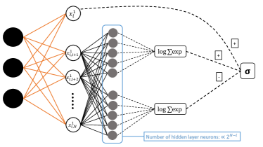
Figure 1: H₂ARNN Architectures of a single Boltzmann conditional probability of a pairwise interacting Hamiltonian, eq.7. The $x_{<i}$ variables are the input, the output is the estimation of the conditional probability $Q^{\theta}(x_{i}=1|\mathbf{x_{<i}})$. The first layer computes the $x^{1}_{i}$ and $x^{1}_{il}$ variables, see eq.8, where the weight and bias, directly related to the Hamiltonian parameters, are shown in orange. The non-linear operators are represented in square form. The width of the second layer grows exponentially with the system size. The last layer is the sigma function.

Then, a second layer acts on the set of $x_{il}^{1}$ (see fig.1). The $\sum_{c}$ is over the $2^{N-i}$ number of configurations of the set of $\mathbf{x}_{>i}$ variables. The parameters of the second layer are

$$b_{c}^{\pm} =\beta\sum_{l=i+1}^{N}(\pm J_{il}+h_{l}+\sum_{l^{\prime}=l+1}^{N}J_{ll^{\prime}}x^{c}_{l^{\prime}})x^{c}_{l}$$ (10)

$$w_{cl} =\beta x^{c}_{l},$$ (11)

where $c$ is the index of the configuration of the set of $\mathbf{x}_{>i}$ variables. Then, the two functions $\rho^{\pm}$ are obtained by applying the non-linear operator $\log\Sigma\exp(\mathbf{x})=\log(\sum_{i}e^{x_{i}})$ at the output of the second layer (see fig.1). As the last layer, the two $\rho^{\pm}$ and $x_{i}^{1}$ are combined with the right signs, and the sigma function is applied. The whole ARNN architecture of the Boltzmann distribution of the general pairwise interacting Hamiltonian ($\text{H}_{2}\text{ARNN}$) is depicted in fig.1. The total number of parameters scales exponentially with the system size, making its direct use infeasible for the sampling process. Nevertheless, the $\text{H}_{2}\text{ARNN}$ architecture shows some interesting features:

• The weights and biases of the first layers are the parameters of the Hamiltonian of the Boltzmann distribution. As far as the author knows, this is the first time that this connection is derived.

• Residual connections among layers, due to the $x_{i}^{1}$ variables, naturally emerge from the derivation. The importance of residual connections has recently been highlighted [47] and has become a crucial element in the success of the ResNet and transformer architectures [48], in classification and generation tasks. They were presented as a way to improve the training of deep neural networks avoiding the exploding and vanishing gradient problem. In our context, they represent the direct interactions among the variable $x_{i}$ and all the previous variables $\mathbf{x}_{<i}$.

• The $\text{H}_{2}\text{ARNN}$ has a recurrent structure [3, 49], similar to some ARNN architectures used in statistical physics problems [27, 31]. The first layer, see figure 1, is composed of the following set of linear operators on the input $x^{1}_{il}(\mathbf{x}_{<i})=\sum_{s=1}^{i-1}J_{si}x_{s}$ with $i<l<=N$. The set of $x_{il}$ can be rewritten in recursive form observing that:

  $$x^{1}_{il}=x^{1}_{i-1,l}+J_{i-1,l}x_{i-1}$$ (12)

  The neurons $x^{1}_{il}$ in the first layer of each conditional probability in the $\text{H}_{2}\text{ARNN}$ architecture depend on the output of the first layer, $x^{1}_{i-1,l}$, of the previous conditional probability.

The number of parameters of the layers of the feed-forward neural network representations of the $\rho_{i}^{\pm}$ functions, eq.6, scale exponentially with the system’s size, proportionally to $2^{N-i}$. The functions $\rho_{i}^{\pm}$ take into account the effect of the interactions among $\mathbf{x}_{<i}$ and $\mathbf{x}_{>i}$ on the variable $x_{i}$. The $\rho_{i}^{\pm}$ function can be interpreted as the partition function of a system, where the variables are the $\mathbf{x}_{>i}$ and the external fields are determined by the values of the variables $\mathbf{x}_{<i}$. Starting from this observation, in the following, I will show how to use standard tools of statistical physics to derive deep AR-NN architectures that eliminates the exponential growth of the number of parameters.

III Models

III.1 The Curie-Weiss model

The Curie-Weiss model (CW) is a uniform, fully-connected Ising model. The Hamiltonian, with $N$ spins, is $H\left(\mathbf{x}\right)=-h\sum_{i=1}^{N}x_{i}-\frac{J}{N}\sum_{i<j}x_{i}x_{j}$. The conditional probability of a spin $i$, eq.5, of the CW model is:

$$P^{CW}\left(x_{i}=1|\mathbf{x}_{<i}\right)=\sigma\bigg{(}2\beta h+2\beta\frac{J}{N}\sum_{s=1}^{i-1}x_{s}+\\ \log(\rho_{i}^{+}[\mathbf{x}_{<i}])-\log(\rho_{i}^{-}[\mathbf{x}_{<i}])\bigg{)},$$ (13)

where:

$$\rho_{i}^{\pm}[\mathbf{x}_{<i}]\propto\sum_{\mathbf{x}_{>i}}e^{\beta\left(h\pm\frac{J}{N}+\frac{J}{N}\sum_{s<i}x_{s}\right)\sum_{l>i}x_{l}+\frac{\beta J}{2N}(\sum_{l,l^{\prime}>i}x_{l}x_{l^{\prime}})}$$ (14)

Defining $h_{i}^{\pm}[\mathbf{x}_{<i}]=h\pm\frac{J}{N}+\frac{J}{N}\sum_{s=1}^{i-1}x_{s}$, at given $\mathbf{x}_{<i}$, eq.14 is equivalent to the partition function of a CW model, with $N-i$ spins and external fields $h_{i}^{\pm}$. As shown in the appendix, the summations over $\mathbf{x_{>i}}$ can be easily done, finding the following expression:

$$\rho_{i}^{\pm}[\mathbf{x}_{<i}]=\sum_{k=0}^{N-i}e^{b_{i,k}^{\pm}+w_{i,k}^{\pm}\sum_{s}x_{s}}$$

where we defined:

$$\begin{split}b_{i,k}^{\pm}&=\log\left(\binom{N-i}{k}\right)+\frac{\beta J}{2N}\left(N-i-2k\right)^{2}+\\ &\qquad\left(N-i-2k\right)\left(\beta h\pm\frac{\beta J}{N}\right)\end{split}$$ (15)

$$\omega_{i,k}^{\pm} =\frac{\beta J}{N}\left(N-i-2k\right).$$ (16)

The final feed-forward architecture of the Curie-Weiss Autoregressive Neural Network (CW_N) architecture is:

$$P^{CW_{N}}\left(x_{i}=+1|\mathbf{x}_{<i}\right)=\sigma\bigg{[}b_{0}+\omega_{0}\sum_{s=1}^{i-1}x_{s}\\ +\log\big{(}\sum_{k=0}^{N-i}e^{b_{i,k}^{+}+w_{i,k}^{+}\sum_{s=1}^{i-1}x_{s}}\big{)}-\log\big{(}\sum_{k=0}^{N-i}e^{b_{i,k}^{-}+w_{i,k}^{-}\sum_{s=1}^{i-1}x_{s}}\big{)}\bigg{]},$$

where $b^{0}=2\beta h$, $\omega^{0}_{i}=\frac{2\beta J}{N}$ are the same, and so shared, among all the conditional probability functions, see fig.2. Their parameters have an analytic dependence on the parameters $J$ and $h$ of the Hamiltonian of the systems.

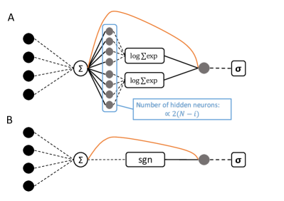
Figure 2: CW_N and CW$\infty$ architectures of a single conditional probability. Diagrams A and B represent the CW_N and CW$\infty$ architectures, respectively. Both diagrams involve the operation of the sum of the input variables $\mathbf{x}_{<i}$. A skip connection, composed of a shared weight (represented by the orange line), is also present in both cases. In the CW_N architecture, $2(N-1)$ linear operations are applied (with fixed weights and biases, as indicated in eq.8), followed by two non-linear operations represented by $\log\sum\exp(x)$. On the other hand, in the CW$\infty$ architecture, apart from the skip connection, the input variables undergo a $sgn$ operation before being multiplied by a free weight parameter and passed through the final layer represented by the sigma function. The number of parameters in the CW_N architecture scales as $2N^{2}+O(N)$, while in the CW$\infty$ architecture, it scales as $N+1$.

The number of parameters of a single conditional probability of the CW_N is $2+4(N-i)$, decreasing as $i$ increases. The CW-ARNN depends only on the sum of the input variables. The total number of parameters of the whole conditional probability distribution scales as $2N^{2}+O(N)$.
If we consider the thermodynamical limit, $N\gg 1$, the ARNN architecture of the CW model, simplify (see sec.IB of the appendix for details) to the following expression:

$$P^{CW_{\infty}}\left(x_{i}=1|\mathbf{x}_{<i}\right)=\sigma\left(b^{0}+\omega_{i}^{0}\sum_{s=1}^{i-1}x_{s}+\omega_{i}^{1}\text{sgn}(\sum_{s=1}^{i-1}x_{s})\right)$$ (17)

where $b^{0}=2\beta h$, $\omega^{0}_{i}=\frac{2\beta J}{N}$ are the same as before, and shared, among all the conditional probability functions. The $\omega^{1}_{i}=-2\beta J|m_{i}|$ is different for each of them and can be computed analytically. The total number of parameters of the CW_∞ scale as $N+2$.

III.2 The Sherrington-Kirkpatrick model

The SK Hamiltonian, with zero external fields for simplicity, is given by:

$$H\left(\mathbf{x}\right)=-\sum_{i<j}J_{ij}x_{i}x_{j}$$ (18)

where the set of couplings, $\underline{J}$, are i.i.d. random variable extracted from a Gaussian probability distribution $P(J)=\mathcal{N}(0,J^{2}/N)$.
To find a feed-forward representation of the conditional probability of its Boltzmann distribution we have to compute the quantities in eq.6, that, defining $h_{l}^{\pm}[\mathbf{x}_{<i}]=\pm J_{il}+\sum_{s=1}^{i-1}J_{sl}x_{s}$, can be written as:

$$\rho_{i}^{\pm}[\mathbf{x}_{<i}]=\sum_{\mathbf{x}_{>i}}\exp\bigg{(}\beta\sum_{l=i+1}^{N}h_{l}^{\pm}[\mathbf{x}_{<i}]x_{l}+\sum_{l^{\prime}>l>i}^{N}J_{ll^{\prime}}x_{l}x_{l^{\prime}}\bigg{)}$$

The above equation can be interpreted as a SK model over the variables $\mathbf{x}_{>i}$ with site depends external fields $h_{l}^{\pm}[\mathbf{x}_{<i}]$. I will use the replica trick [50], which is usually applied together with the average over the system’s disorder. In our case, we deal with a single instance of disorder, the set of couplings is fixed. In the following I will assume that $N-i\gg 1$, and the average over the disorder $\mathbb{E}$ is taken on the coupling parameters $J_{ll^{\prime}}$ with $l,l^{\prime}>i$. In practice I will use the following approximation to compute the quantity:

$$\log\rho_{i}^{\pm}\sim\mathbb{E}\left[\log\rho_{i}^{\pm}\right]=\lim_{n\rightarrow 0}\frac{\log(\mathbb{E}\left[(\rho_{i}^{\pm})^{n}\right])}{n}$$

In the last equality, I use the replica trick. Implicitly, I assume that the quantities $\log\rho_{i}^{\pm}$ are self-averaged on the $\mathbf{x}_{>i}$ variables. The expression of the average over the disorder of the replicated function is:

$$\mathbb{E}_{\underline{J}_{ll^{\prime}}}\left[(\rho_{i}^{\pm}[\mathbf{x}_{<i}])^{n}\right]=\int\prod_{l<l^{\prime}}dP_{J_{ll^{\prime}}}\bigg{\{}\sum_{\{\underline{x}^{a}\}_{i+1}^{N}}\exp\bigg{[}\\ \beta\bigg{(}\sum_{\begin{subarray}{c}i<l\leq N\\ 1<a<n\end{subarray}}h_{l}^{\pm}[\mathbf{x}_{<i}]x_{l}^{a}+\sum_{\begin{subarray}{c}i<l<l^{\prime}\leq N\\ 1<a\leq n\end{subarray}}J_{ll^{\prime}}x_{l}^{a}x_{l^{\prime}}^{a}\bigg{)}\bigg{]}\bigg{\}}$$ (19)

where $dP_{J_{ll^{\prime}}}=P(J_{ll^{\prime}})dJ_{ll^{\prime}}$. Computing the integrals over the disorder, we find:

$$\mathbb{E}_{\underline{J}_{ll^{\prime}}}\left[(\rho_{i}^{\pm}[\mathbf{x}_{<i}])^{n}\right] \propto\int\prod_{a<b}dQ_{ab}e^{-\frac{N}{2}\beta^{2}Q_{a,b}^{2}}\prod_{l}\left[\sum_{\{\underline{x}^{a}_{l}\}}\exp\left\{\beta\left[h_{l}^{\pm}[\mathbf{x}_{<i}]\sum_{a}x_{l}^{a}+\beta\sum_{a<b}Q_{a,b}x_{l}^{a}x_{l}^{b}\right]\right\}\right]$$ (20)

where in the last line I used the Hubbard-Stratonovich transformation to linearize the quadratic terms. The Parisi solutions of the SK model prescribe how to parametrize the matrix of the overlaps $\{Q_{a,b}\}$ [50]. The easiest way to parametrize the matrix of the overlaps is the replica symmetric solutions (RS), where the overlaps are equal and independent from the replica index:

$$Q_{a,b}=\begin{cases}0,&\text{if $a=b$}\\ q,&\text{otherwise}\end{cases},$$

Then a sequence of better approximations can be obtained by breaking, by step, the replica symmetry, from the 1-step replica symmetric breaking (1-RSB) to k-step replica symmetric breaking (k-RSB) solutions. The infinite k-step limit of k-step replica symmetric breaking solution gives the exact solution of the SK model [51]. The sequence of k-RSB approximations can be seen as nested non-linear operations [52], see appendix for details.

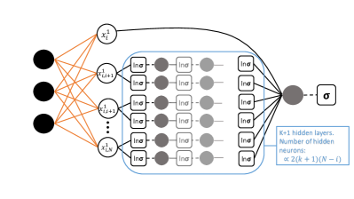
Figure 3: SK_RS/kRSB architectures of a single conditional probability [CHECK] The diagram depicts the SK_RS/kRSB architectures that approximate a single conditional probability of the Boltzmann distribution in the SK model. The input variables are $\mathbf{x}_{<i}$, while the output is the conditional probability $Q^{\text{RS/k-RSB}}\left(x_{i}=1|\mathbf{x}_{<i}\right)$. The non-linear operations are represented by squares and the linear operations by solid lines. The parameters, in the orange lines, are equal to the Hamiltonian parameters and shared among the conditional probabilities, as indicated in equation 8. The depth of the network is determined by the level of approximation used, with the $Q^{\text{RS}}$ architecture having only one hidden layer and the $Q^{\text{k-SRB}}$ architecture having a sequence of $k+1$ hidden layers. The total number of parameters scales as $2(k+1)N^{2}+\mathbb{O}(N)$, where the $RS$ case corresponds to $k=0$.

Every k-step replica symmetric breaking solution leads to adding a Gaussian integral and two more free variational parameters to the representation of the $\rho^{\pm}$ functions. In the following, we will use a feed-forward representation that enlarges the space of parameters, using a more computationally friendly non-linear operator. Numerical evidence of the quality of the approximation used is shown in the appendix. Overall, the parametrization of the overlaps matrix allows to perform the sum over all the configurations of the variables $\mathbf{x}_{i>}$ getting rid of the exponential scaling with the system’s size of the number of parameters. The final AR-NN architecture of the SK model (SK-ARNN) is, see appendix for details,

$$Q^{\text{RS/k-RSB}}\left(x_{i}=1|\mathbf{x}_{<i}\right)=\sigma\bigg{(}x_{i}^{1}(\mathbf{x}_{<i})\\ +\log(\rho_{i}^{+,\text{(RS/kRSB)}})-\log(\rho_{i}^{-,\text{(RS/kRSB)}})\bigg{)}.$$ (21)

For RS and 1-RSB cases we have:

$$\log\rho^{\pm,RS} =\sum_{l^{\pm}=i+1}^{N}w_{0}^{i,l^{+}}\log\sigma(b_{1}^{i,l^{\pm}}+w_{1}^{i,l^{\pm}}x_{i,l^{\pm}}^{1}(\mathbf{x}_{<i}))$$

$$\begin{split}\log\rho^{\pm,1RSB}&=\sum_{l^{\pm}=i+1}^{N}w_{0}^{i,l^{\pm}}\log\sigma(b_{1}^{i,l^{\pm}}+\\ &w_{1}^{i,l^{\pm}}\log\sigma(b_{2}^{i,l^{\pm}}+w_{2}^{i,l^{\pm}}x_{i,l^{\pm}}^{1}(\mathbf{x}_{<i}))).\end{split}$$

The set of $x_{i,l^{\pm}}^{1}(\mathbf{x}_{<i})$ is the output of the first layer of the ARNN, see eqs.8-9, and $(w_{0}^{i,l^{\pm}},b_{1}^{i,l^{\pm}},w_{1}^{i,l^{\pm}},b_{2}^{i,l^{\pm}},w_{2}^{i,l^{\pm}})$ are free variational parameters of the ARNN, see fig.3. The number of parameters of a single conditional probability distribution scales as $2(k+1)(N-i)$ where $k$ is the level of the k-RSB solution used, assuming $k=0$ as the RS solution.

IV Results

In this section, I compare several ARNN architectures in learning to generate samples from the Boltzmann distribution of the CW and SK models. Moreover, the ability to recover the Hamiltonian coupling parameters from Monte-Carlo-generated instances is presented. The CW_N, CW_∞ and SK_RS/kRSB architectures, presented in previous sections, are compared with:

• The one parameter (1P) architecture, where a single weight parameter is multiplied by the sums of the input variables, and then the sigma function is applied. This architecture was already used for the CW system in [36]. The total number of parameters scales as $N$.

• The single layer (1L) architecture, where a fully connected single linear layer parametrizes the whole probability distribution, where a mask is applied to a subset of the weights in order to preserve the autoregressive properties. The width of the layer is $N$, and the total number of parameters scale as $N^{2}$ [15].

• The MADE architecture[15], where the whole probability distribution is represented with a deep sequence of fully connected layers, with non-linear activation functions and masks in between them, to assure the autoregressive properties. Respect the 1L the deep architecture of MADE enhances the expressive power. The MADE_dw used has $d$ hidden layers, each of them with width $w$ times the input variables $N$. For instance, the 1L architecture is equivalent to the MADE₁₁ and MADE₂₃ has two hidden fully-connected layers, each of them of width $3N$.

The parameters of the ARNN are trained using the Kullback-Leibler divergence or equivalently the variational free energy, see equation 1. Given an ARNN, $Q^{\theta}$, that depend on a set of parameters $\theta$ and the Boltzmann distribution $P$, the variational free energy can be estimates as:

$$F[Q^{\theta}] =\sum_{\left\{\mathbf{x}\right\}}Q^{\theta}\left[\frac{1}{\beta}\log Q^{\theta}+H[\mathbf{x}]\right]$$

$$\approx\sum_{\mathbf{x}\sim Q^{\theta}}\left[\frac{1}{\beta}\log Q^{\theta}+H[\mathbf{x}]\right].$$

The samples are extracted, thanks to the ancestral sampling, from the ARNN $Q^{\theta}$. At each step of the training, the derivative of the variational free energy with respect to the parameters $\theta$ is estimated and used to update the parameters of the ARNN. Then a new batch of samples is extracted from the ARNN and used again to compute the derivative of the variational free energy and update the parameters[8]. This process was repeated until a stop criterion is meet or a maximum number of steps is reached. For each model and temperature, a maximum number of $1000$ epochs are allowed, with a batch size of $2000$ samples, and a learning rate of $0.001$. The ADAM algorithm[53] was applied for the optimization of the ARNN parameters. An annealing procedure was used to improve the performances and avoid mode-collapse problems[8], where the inverse temperature $\beta$ was increased from $0.1$ to $2.0$ with a step of $0.05$. The code was written using the PyTorch framework[54], and it is open-source, released in [55].

The CW_N has all its parameters fixed and precomputed analytically, see eq.15. The CW_∞ has one free parameter for each of its conditional probability distributions, and 1 shared parameter to be trained, see eq.17. The parameters of the first layer of the SK_RS/kRSB architecture are shared and fixed by the values of the couplings and fields of the hamiltonian. The parameters of the hidden layers are free and trained. The parameters of the MADE_dw, 1L and 1P architectures are free and trained.

As explained in sec.II, the variational free energy $F[Q^{\theta}]$ is always an upper bound of the free energy of the system, and its values will be used, in the following, as a benchmark of the performance of the ARNN architecture tested to approximate the Boltzmann distribution; after the training procedure, the variational free energy was estimated using 20,000 configurations sampled from each of the ARNN architecture considered. The training procedure was the same for all the experiments unless conversely specified.

CW model

The results on the CW model, with $J=1$ and $h=0$, are shown in fig.4.

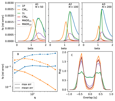
Figure 4: Results for CW model. The CW model considered has $J=1$ and $h=0$ (see the text for details). The system undergoes a second-order phase transition at $\beta=1$ where a spontaneous magnetization appears[37]. [A1, A2, A3] Relative error in the estimation of the free energy for different system sizes with respect to the analytic solution. [B] Scaling with $N$ of the mean and max relative error of the two smaller architecture $1P$ and CW_∞, both scaling linearly with the system’s size. [C] Distribution of the overlaps of the samples generated by the ARNNs for the CW system with $N=200$ variables and $\beta=1.3$

The plots A1, A2, and A3, in the first row, show the relative error of the free energy density ($fe[P]=F[P]/N$), with respect to the exact one, computed analytically [37], see appendix for details, for different system sizes $N$. The variational free energy density estimated from samples generated with the CW_N architecture does not have an appreciable difference with the analytic solution, and for the CW_∞, it improves as the system size increases. Fig.4.B plots the error, in the estimation of the free energy density for the architectures with fewer parameters, 1P and CW_∞ (both scaling linearly with the system’s size); It shows clearly that a deep architecture, in this case with only one more parameter, improves the accuracy by orders of magnitude. The need for deep architectures, already on a simple model as the CW, is indicated by the poor performance of the 1L architecture, despite its scaling of parameters as $N^{2}$, it achieves similar results to the 1P. The MADE architecture obtains good results but was not comparable to CW_N, even though having a similar number of parameters. The plot in fig.4.c shows the distribution of the overlaps, $q_{\mathbf{a},\mathbf{b}}=\frac{1}{N}\sum_{i}a_{i}b_{i}$ where $a_{i},b_{i}$ are two system configurations, between the samples generated by the ARNNs. The distribution is computed at $\beta=1.3$ for $N=200$. It can be seen as the poor performance of the 1-layer networks (1P, 1L) is due to the difficulty of correctly representing the configurations with magnetization different from zero in the proximity of the phase transition. This could be due to mode collapse problems [36], which do not affect the deeper ARNN architectures tested.

SK model

In figure 5, the result of the SK model, with $J=1$ and $h=0$ are shown; as before in the first row there is the relative error in the estimation of the free energy density at different system sizes.

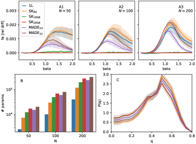
Figure 5: Results for SK model. The SK model considered has $J=1$ and $h=0$ (see the text for details). The system undergoes a phase transition at $\beta=1$[50]. [A1, A2, A3] Relative difference in the estimation of the free energy for increasing system sizes with respect to the free energy computed by SK_2RSB architecture. The results are averaged over 10 instances of the disorder. [B] Scaling with $N$ of the number of parameters of the ARNN architectures. [C] Distribution of the overlaps of the samples generated by the ARNNs architectures for the SK model with $N=200$ variables and $\beta=1.5$, averaged over 10 different instances.

In this case, the exact solution, for a single instance of the disorder and a finite $N$ is not known. The free energy estimation of the SK_2RSB was taken as the reference to compute the relative difference. The free energy estimations of SK_kRSB with $k=1,2$ are very close to each other. The performance of the SK_RS net is the same as the 1L architecture even with a much higher number of parameters. The MADE architecture tested, even with a similar number of parameters of the SK_kRSB nets, see fig.5.C, estimate a larger free energy, with differences increasing with $N$. To better assess the difference in the approximation of the Boltzmann distribution of the architecture tested, I consider to check the distributions of the overlaps $q$ among the generated samples. The SK model, with $J=1$ and $h=0$, undergo a phase transition at $\beta=1$, where a glassy phase is formed, and an exponential number of metastable states appears [50]. This fact is reflected in the distribution of overlaps that have values different from zero in a wide region of values of $q$ [56]. Observing the distribution of the overlaps in the glassy phase, $\beta=1.3$, between the samples generated by the ARNNs, fig.5.D, we can check as the distribution generated by the SK_kRSB is higher in the region between the peak and zero overlaps, suggesting that these architectures better capture the complex landscape of the SK Boltzmann probability distribution [56].

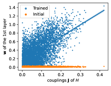
Figure 6: Scatter plot of the weights vs the coupling. Scatter plot of the absolute values of weights of the first layer of a SK_1RSB vs the absolute values of the coupling parameters of the SK model. The weights are trained over 10,000 samples generated by the Metropolis Monte Carlo algorithm on a single instance of the SK model with $N=100$ variables at $\beta=2$. They are initialized at small random values. The blue line is the fit of the blue points, clearly showing a strong correlation between the weights and the coupling parameters of the Hamiltonian.

The final test for the derived SK_kRSB architectures involves evaluating the ability to recover the Hamiltonian couplings of the system using only samples extracted from the Boltzmann distribution of a single instance of the SK model. 10,000 samples were generated using the Metropolis Monte-Carlo algorithm and the SK_1RSB was trained to minimize the log-likelihood computed on these samples (see SI for details). According to the derivation of the SK_kRSB architecture, the weights of the first layer of the neural network should correspond to the coupling parameters of the Hamiltonian. Due to the gauge invariance of the Hamiltonian with respect to the change of sign of all the couplings $J$s, I will consider their absolute values in the comparison. The weights parameters of the first layers of the SK_1RSB were initialized at small random values. As shown in Fig.6, there is a strong correlation between the weights of the first layer and the couplings of the Hamiltonian, even though the neural network was trained in an over-parameterized setting; it has 60,000 parameters, significantly more than the number of samples.

V Conclusions

In this study, the exact architecture Autoregressive Neural Network (ARNN) architecture (H₂ARNN) of the Boltzmann distribution of the pairwise interacting system Hamiltonian was derived. The H₂ARNN is a deep neural network, with the weights and biases of the first layer corresponding to the couplings and external fields of the Hamiltonian, see eqs.8-9. The H₂ARNN architecture has skip-connections and a recurrent structure with a clear physical interpretation. Although the H₂ARNN is not directly usable due to the exponential increase in the number of hidden layer parameters with the size of the system, its explicit formulation allows using statistical physics techniques to derive tractable architectures for specific problems. For example, ARNN architectures, scaling polynomially with the system’s size, are derived for the CW and SK models. In the case of the SK model, the derivation is based on the sequence of k-step replica symmetric breaking solutions, which were mapped to a sequence of deeper ARNNs architectures.

The results, checking the ability of the ARNN architecture to learn the Boltzmann distribution of the CW and SK models, indicate that the derived architectures outperform commonly used ARNNs. Furthermore, the close connection between the physics of the problem and the neural network architecture is shown in the results of fig.6. In this case, the SK_1RSB architecture was trained on samples generated with Monte-Carlo technique from the Boltzmann distribution of an SK model; the weights of the first layer of the SK_1RSB were found to have a strong correlation with the coupling parameters of the Hamiltonian.

Even though the derivation of a simple and compact ARNN architecture is not always feasible for all types of pairwise interactions and exactly solvable physics systems are rare, the explicit form of the H₂ARNN and its clear physical interpretation provides a means to derive approximate architectures for specific Boltzmann distributions.
In this work, while the ARNN architecture of an SK model was derived, its learnability was not thoroughly examined. The problem of finding the configurations of minimum energy for the SK model is known to belong to the NP-hard class, and the effectiveness of the ARNN approach in solving this problem is still uncertain and a matter of ongoing research [36, 27, 35]. Further systematic studies are needed to fully understand the learnability of the ARNN architecture presented in this work at very low temperatures and also on different systems.

There are several promising directions for future research to expand upon presented ARNN architectures. For instance, deriving the architecture for statistical models with more than binary variables. In statistical physics, the models with variables that have more than two states are called Potts models. The language models, where each variable represents a word, and could take values among a huge number of states, usually more than tens of thousand possible words (or states), belong to this set of systems. The generalization of the present work to Potts models could allow us to connect the physics of the problem to recent language generative models like the transformer architecture [18]. Another direction could be to consider systems with interactions beyond pairwise, to describe more complex probability distributions. Additionally, it would be interesting to examine sparse interacting system graphs, such as systems that interact on grids or random sparse graphs. The first case is fundamental for a large class of physics systems and image generation tasks, while the latter type, such as Erdos-Renyi interaction graphs, is common in optimization [44] and inference problems [57].

References

- Hopfield [1982] J. J. Hopfield, Neural networks and physical systems with emergent collective computational abilities., Proceedings of the National Academy of Sciences 79, 2554 (1982), https://www.pnas.org/doi/pdf/10.1073/pnas.79.8.2554 .
- Amit et al. [1985a] D. J. Amit, H. Gutfreund, and H. Sompolinsky, Spin-glass models of neural networks, Phys. Rev. A 32, 1007 (1985a).
- LeCun et al. [2015] Y. LeCun, Y. Bengio, and G. Hinton, Deep learning, Nature 521, 436 (2015).
- Carleo et al. [2019] G. Carleo, I. Cirac, K. Cranmer, L. Daudet, M. Schuld, N. Tishby, L. Vogt-Maranto, and L. Zdeborová, Machine learning and the physical sciences, Rev. Mod. Phys. 91, 045002 (2019).
- Carleo and Troyer [2017] G. Carleo and M. Troyer, Solving the quantum many-body problem with artificial neural networks, Science 355, 602 (2017), https://www.science.org/doi/pdf/10.1126/science.aag2302 .
- van Nieuwenburg et al. [2017] E. P. L. van Nieuwenburg, Y.-H. Liu, and S. D. Huber, Learning phase transitions by confusion, Nature Physics 13, 435 (2017).
- Carrasquilla and Melko [2017] J. Carrasquilla and R. G. Melko, Machine learning phases of matter, Nature Physics 13, 431 (2017).
- Wu et al. [2019] D. Wu, L. Wang, and P. Zhang, Solving Statistical Mechanics Using Variational Autoregressive Networks, Physical Review Letters 122, 1 (2019), 1809.10606 .
- Noé et al. [2019] F. Noé, S. Olsson, J. Köhler, and H. Wu, Boltzmann generators: Sampling equilibrium states of many-body systems with deep learning, Science 365, eaaw1147 (2019).
- Jumper et al. [2021] J. Jumper, R. Evans, A. Pritzel, T. Green, M. Figurnov, O. Ronneberger, K. Tunyasuvunakool, R. Bates, A. Žídek, A. Potapenko, et al., Highly accurate protein structure prediction with alphafold, Nature 596, 583 (2021).
- Zdeborová and Krzakala [2016] L. Zdeborová and F. Krzakala, Statistical physics of inference: thresholds and algorithms, Advances in Physics 65, 453 (2016), https://doi.org/10.1080/00018732.2016.1211393 .
- Nguyen et al. [2017] H. C. Nguyen, R. Zecchina, and J. Berg, Inverse statistical problems: from the inverse ising problem to data science, Advances in Physics, Advances in Physics 66, 197 (2017).
- Chaudhari et al. [2019] P. Chaudhari, A. Choromanska, S. Soatto, Y. LeCun, C. Baldassi, C. Borgs, J. Chayes, L. Sagun, and R. Zecchina, Entropy-sgd: biasing gradient descent into wide valleys*, Journal of Statistical Mechanics: Theory and Experiment 2019, 124018 (2019).
- Sohl-Dickstein et al. [2015] J. Sohl-Dickstein, E. Weiss, N. Maheswaranathan, and S. Ganguli, Deep unsupervised learning using nonequilibrium thermodynamics, in Proceedings of the 32nd International Conference on Machine Learning, Proceedings of Machine Learning Research, Vol. 37, edited by F. Bach and D. Blei (PMLR, Lille, France, 2015) pp. 2256–2265.
- Germain et al. [2015] M. Germain, K. Gregor, I. Murray, and H. Larochelle, Made: Masked autoencoder for distribution estimation, in Proceedings of the 32nd International Conference on Machine Learning, Proceedings of Machine Learning Research, Vol. 37, edited by F. Bach and D. Blei (PMLR, Lille, France, 2015) pp. 881–889.
- van den Oord et al. [2016a] A. van den Oord, N. Kalchbrenner, L. Espeholt, k. kavukcuoglu, O. Vinyals, and A. Graves, Conditional image generation with pixelcnn decoders, in Advances in Neural Information Processing Systems, Vol. 29, edited by D. Lee, M. Sugiyama, U. Luxburg, I. Guyon, and R. Garnett (Curran Associates, Inc., 2016).
- Vaswani et al. [2017a] A. Vaswani, N. Shazeer, N. Parmar, J. Uszkoreit, L. Jones, A. N. Gomez, L. u. Kaiser, and I. Polosukhin, Attention is all you need, in Advances in Neural Information Processing Systems, Vol. 30, edited by I. Guyon, U. V. Luxburg, S. Bengio, H. Wallach, R. Fergus, S. Vishwanathan, and R. Garnett (Curran Associates, Inc., 2017).
- Brown et al. [2020] T. B. Brown, B. Mann, N. Ryder, M. Subbiah, J. Kaplan, P. Dhariwal, A. Neelakantan, P. Shyam, G. Sastry, A. Askell, S. Agarwal, A. Herbert-Voss, G. Krueger, T. Henighan, R. Child, A. Ramesh, D. M. Ziegler, J. Wu, C. Winter, C. Hesse, M. Chen, E. Sigler, M. Litwin, S. Gray, B. Chess, J. Clark, C. Berner, S. McCandlish, A. Radford, I. Sutskever, and D. Amodei, Language models are few-shot learners (2020).
- Gregor et al. [2014] K. Gregor, I. Danihelka, A. Mnih, C. Blundell, and D. Wierstra, Deep autoregressive networks, in Proceedings of the 31st International Conference on Machine Learning, Proceedings of Machine Learning Research, Vol. 32, edited by E. P. Xing and T. Jebara (PMLR, Bejing, China, 2014) pp. 1242–1250.
- Larochelle and Murray [2011] H. Larochelle and I. Murray, The neural autoregressive distribution estimator, in Proceedings of the Fourteenth International Conference on Artificial Intelligence and Statistics, Proceedings of Machine Learning Research, Vol. 15, edited by G. Gordon, D. Dunson, and M. Dudík (PMLR, Fort Lauderdale, FL, USA, 2011) pp. 29–37.
- van den Oord et al. [2016b] A. van den Oord, N. Kalchbrenner, and K. Kavukcuoglu, Pixel recurrent neural networks, in Proceedings of The 33rd International Conference on Machine Learning, Proceedings of Machine Learning Research, Vol. 48, edited by M. F. Balcan and K. Q. Weinberger (PMLR, New York, New York, USA, 2016) pp. 1747–1756.
- Nash and Durkan [2019] C. Nash and C. Durkan, Autoregressive energy machines, in Proceedings of the 36th International Conference on Machine Learning, Proceedings of Machine Learning Research, Vol. 97, edited by K. Chaudhuri and R. Salakhutdinov (PMLR, 2019) pp. 1735–1744.
- Nicoli et al. [2020] K. A. Nicoli, S. Nakajima, N. Strodthoff, W. Samek, K.-R. Müller, and P. Kessel, Asymptotically unbiased estimation of physical observables with neural samplers, Physical Review E 101, 023304 (2020), 1910.13496 .
- McNaughton et al. [2020] B. McNaughton, M. V. Milošević, A. Perali, and S. Pilati, Boosting monte carlo simulations of spin glasses using autoregressive neural networks, Phys. Rev. E 101, 053312 (2020).
- Pan et al. [2021] F. Pan, P. Zhou, H.-J. Zhou, and P. Zhang, Solving statistical mechanics on sparse graphs with feedback-set variational autoregressive networks, Phys. Rev. E 103, 012103 (2021).
- Wu et al. [2021] D. Wu, R. Rossi, and G. Carleo, Unbiased monte carlo cluster updates with autoregressive neural networks, Phys. Rev. Res. 3, L042024 (2021).
- Hibat-Allah et al. [2021] M. Hibat-Allah, E. M. Inack, R. Wiersema, R. G. Melko, and J. Carrasquilla, Variational neural annealing, Nature Machine Intelligence 3, 1 (2021), 2101.10154 .
- Luo et al. [2022] D. Luo, Z. Chen, J. Carrasquilla, and B. K. Clark, Autoregressive Neural Network for Simulating Open Quantum Systems via a Probabilistic Formulation, Physical Review Letters 128, 090501 (2022).
- Wang and Davis [2020] Z. Wang and E. J. Davis, Calculating rényi entropies with neural autoregressive quantum states, Phys. Rev. A 102, 062413 (2020).
- Sharir et al. [2020] O. Sharir, Y. Levine, N. Wies, G. Carleo, and A. Shashua, Deep autoregressive models for the efficient variational simulation of many-body quantum systems, Phys. Rev. Lett. 124, 020503 (2020).
- Hibat-Allah et al. [2020] M. Hibat-Allah, M. Ganahl, L. E. Hayward, R. G. Melko, and J. Carrasquilla, Recurrent neural network wave functions, Phys. Rev. Res. 2, 023358 (2020).
- Liu et al. [2021] J.-G. Liu, L. Mao, P. Zhang, and L. Wang, Solving quantum statistical mechanics with variational autoregressive networks and quantum circuits, Machine Learning: Science and Technology 2, 025011 (2021).
- Barrett et al. [2022] T. D. Barrett, A. Malyshev, and A. I. Lvovsky, Autoregressive neural-network wavefunctions for ab initio quantum chemistry, Nature Machine Intelligence 4, 351 (2022).
- Cha et al. [2021] P. Cha, P. Ginsparg, F. Wu, J. Carrasquilla, P. L. McMahon, and E.-A. Kim, Attention-based quantum tomography, Machine Learning: Science and Technology 3, 01LT01 (2021).
- Inack et al. [2022] E. M. Inack, S. Morawetz, and R. G. Melko, Neural annealing and visualization of autoregressive neural networks in the newman-moore model, Condensed Matter 7, 10.3390/condmat7020038 (2022).
- Ciarella et al. [2022] S. Ciarella, J. Trinquier, M. Weigt, and F. Zamponi, Machine-learning-assisted monte carlo fails at sampling computationally hard problems (2022).
- Kadanoff [2000] L. P. Kadanoff, Statistical physics: statics, dynamics and renormalization (World Scientific, 2000).
- Sherrington and Kirkpatrick [1975] D. Sherrington and S. Kirkpatrick, Solvable model of a spin-glass, Phys. Rev. Lett. 35, 1792 (1975).
- nobel committee for Physics [2021] T. nobel committee for Physics, For groundbreaking contributions to our understanding of complex physical systems. [nobel to g. parisi] (2021).
- Parisi [1979a] G. Parisi, Toward a mean field theory for spin glasses, Physics Letters A 73, 203 (1979a).
- Parisi [1979b] G. Parisi, Infinite number of order parameters for spin-glasses, Phys. Rev. Lett. 43, 1754 (1979b).
- Gardner [1987] E. Gardner, Maximum storage capacity in neural networks, Europhysics Letters 4, 481 (1987).
- Amit et al. [1985b] D. J. Amit, H. Gutfreund, and H. Sompolinsky, Storing infinite numbers of patterns in a spin-glass model of neural networks, Phys. Rev. Lett. 55, 1530 (1985b).
- Mézard et al. [2002] M. Mézard, G. Parisi, and R. Zecchina, Analytic and algorithmic solution of random satisfiability problems, Science , 812 (2002), https://www.science.org/doi/pdf/10.1126/science.1073287 .
- Parisi and Zamponi [2010] G. Parisi and F. Zamponi, Mean-field theory of hard sphere glasses and jamming, Rev. Mod. Phys. 82, 789 (2010).
- Biazzo et al. [2009] I. Biazzo, F. Caltagirone, G. Parisi, and F. Zamponi, Theory of amorphous packings of binary mixtures of hard spheres, Phys. Rev. Lett. 102, 195701 (2009).
- He et al. [2015] K. He, X. Zhang, S. Ren, and J. Sun, Deep Residual Learning for Image Recognition, arXiv 10.48550/arxiv.1512.03385 (2015), 1512.03385 .
- Vaswani et al. [2017b] A. Vaswani, N. Shazeer, N. Parmar, J. Uszkoreit, L. Jones, A. N. Gomez, Ł. Kaiser, and I. Polosukhin, Attention is all you need, Advances in neural information processing systems 30 (2017b).
- Lipton et al. [2015] Z. C. Lipton, J. Berkowitz, and C. Elkan, A critical review of recurrent neural networks for sequence learning (2015).
- Mezard et al. [1986] M. Mezard, G. Parisi, and M. Virasoro, Spin Glass Theory and Beyond (1986).
- Talagrand [2006] M. Talagrand, The parisi formula, Annals of Mathematics 163, 221 (2006).
- Parisi [1980] G. Parisi, A sequence of approximated solutions to the s-k model for spin glasses, Journal of Physics A: Mathematical and General 13, L115 (1980).
- Kingma and Ba [2014] D. P. Kingma and J. Ba, Adam: A method for stochastic optimization, arXiv preprint arXiv:1412.6980 (2014).
- Paszke et al. [2019] A. Paszke, S. Gross, F. Massa, A. Lerer, J. Bradbury, G. Chanan, T. Killeen, Z. Lin, N. Gimelshein, L. Antiga, A. Desmaison, A. Kopf, E. Yang, Z. DeVito, M. Raison, A. Tejani, S. Chilamkurthy, B. Steiner, L. Fang, J. Bai, and S. Chintala, Pytorch: An imperative style, high-performance deep learning library, in Advances in Neural Information Processing Systems, Vol. 32, edited by H. Wallach, H. Larochelle, A. Beygelzimer, F. d'Alché-Buc, E. Fox, and R. Garnett (Curran Associates, Inc., 2019).
- Biazzo [2023] I. Biazzo, h2arnn, http://github.com/ocadni/h2arnn (2023), [Online; accessed 9-march-2023].
- Young [1983] A. P. Young, Direct determination of the probability distribution for the spin-glass order parameter, Phys. Rev. Lett. 51, 1206 (1983).
- Biazzo et al. [2022] I. Biazzo, A. Braunstein, L. Dall’Asta, and F. Mazza, A bayesian generative neural network framework for epidemic inference problems, Scientific Reports 12, 19673 (2022).