On blowups of vorticity for the homogeneous Euler equation

Abstract

Blowups of vorticity for the three- and two- dimensional homogeneous Euler equations are studied. Two regimes of approaching a blowup points, respectively, with variable or fixed time are analysed. It is shown that in the $n$-dimensional ($n=2,3$) generic case the blowups of degrees $1,..,n$ at the variable time regime and of  degrees $1/2,..,(n+1)/(n+2)$ at the fixed time regime may exist.  Particular situations when the vorticity blows while the direction of the vorticity vector is concentrated in one or two directions are realisable.

1 Introduction

Vorticity and associated phenomena are among the most studied subjects in hydrodynamics (see e.g. [18, 20, 2, 21, 19] and the papers [6, 5, 22, 3, 4, 13, 14, 15, 16, 17]). Number of approaches and different techniques have been developed. Most of the studies of the blowups of vorticity has been performed for the ideal incompressible fluid. The compressible case is considered as the much more complicated one (see e.g. [18, 20, 2, 21, 19, 6, 5, 22]).

In the papers [3] and [16] it was observed that in the case of compressible fluid the behavior of vorticity for the Euler equation is intimately connected with that of homogeneous Euler equation (HEE)

$${\mathbf{u}}_{t}+{\mathbf{u}}\cdot\nabla{\mathbf{u}}=0\,.$$ (1.1)

without the constraint $\nabla\cdot{\mathbf{u}}=0$. In the papers [3, 4] an explicit integral-type formula for the vorticity $\bm{\omega}=\nabla\times{\mathbf{u}}$ for the equation (1.1) has been presented. Another type of formula for the vorticity has been found in [13, 14]. The blowup of vorticity as $t\to t_{c}>0$ has been analysed in [14, 16] (see also [4] and [17]).

Homogeneous Euler equation (1.1) is the most simplified version of the basic equations of the hydrodynamics when one can neglect all effects of pressure, viscosity etc.. Nevertheless it has number of applications in physics and represent itself an excellent touchstone for an analysis of blowups of vorticity.

In this paper we present some results concerning the blowups of vorticity for the three- and two-dimensional homogeneous Euler equation (1.1). Our analysis is based in part on the previous study of the structure and hierarchies of blowups of derivatives for the $n$-dimensional HEE [10, 11].

We consider the behavior of vorticity in two different regimes of approaching the blowup points at the blowup hypersurface. The first regime is to approach such a point along the $t$ axis, i.e. $t\to t_{b}$ while the coordinates ${\mathbf{u}}$ in the hodograph space remain fixed. It is shown that, in the generic case, i.e. for generic initial data for the 3D HEE (1.1), the vorticity in this regime may have singularities of three different degrees

$$\omega_{i}\sim(t-t_{b})^{-m}\,,\qquad t\to t_{b},\qquad m=1,2,3\,.$$ (1.2)

Such blowups occur on the intersection of $m$ branches of the blowup hypersurface $\Gamma$. The existence of blowups of type (1.2) with $m=1,2$ has been observed earlier in [14].

In the second regime the time $t_{b}$ is fixed while the coordinates ${\mathbf{u}}$ are variyng. In this regime of approaching the blowup point for 3D HEE (1.1) generically it may exists 4 levels of blowups of the vorticity $\bm{\omega}$ with the behavior

$$\omega_{i}\sim\epsilon^{-\frac{m}{m+1}}\,,\qquad m=1,2,3,4\,,$$ (1.3)

where $\epsilon\sim|\delta{\mathbf{x}}|\to 0$. Blowups (1.3) occur on the subspaces $\Gamma_{m}$ of the blowup hypersurface $\Gamma$ and dim$\Gamma_{m}=4-m$, $m=1,2,3,4$.

It may happens also that the components of the vorticity $\bm{\omega}$ behave differently on certain subspaces of $\Gamma$. In particular, at the first level $m=1$ there may exist one-dimensional subspace ${\Gamma}_{1}$ at which the component $\omega_{3}$ blows as $\epsilon^{-1/2}$ when $\epsilon\to 0$ while the components $\omega_{1}$ and $\omega_{2}$ remain bounded. In such a case the direction of the vorticity $\bm{\hat{\omega}}$ is a unit vector oriented along one axes, namely

$$\bm{\hat{\omega}}=\big{(}0,0,1\big{)}\,.$$ (1.4)

The calculations are performed both in the special coordinates introduced in [11] as well as in cartesian coordinates ${\mathbf{x}}$ and ${\mathbf{u}}$.

For the 2D HEE (1.1) the vorticity blows-up as in (1.2) and (1.3) with $m$ taking the values $m=1,2$ for (1.2) and $m=1,2,3$ for (1.3), respectively. Three particular solutions of the 2D HEE with different blowup behavior are considered.

It is noted that we analyze the behavior of vorticity at certain points on the blowup hypersurface $\Gamma$ and at the time $t_{b}$ which can be negative or positive. The realisability of blowups of different orders at positive time remains an open problem.

Similar results for the $n$-dimensional homogeneous Euler equation are briefly discussed too.

The paper is organized as follows. Section 2 contains a brief exposition of the results of the paper [11] for the 3D HEE. Blowups of vorticity in the first regime $t\to t_{b}$ are analysed in section 3. Blowups of vorticity for the 3D HEE in the regime with fixed $t$ are studied in sections 4 and 5. Similar results for the 2D HEE are presented in section 6. Three particular solutions of the 2D HEE with different blowup behavior are described in detail in Section 7. The $n$-dimensional $n\geq 4$ case is discussed in Section 8. Conclusion 9 contains some indications on possible future developments.

2 Blowups of derivatives

Here for conveniency we report some results concerning the blowup of derivatives for the 3-dimensional homogeneous Euler equation obtained in the paper [11]. We also slightly change the notations in order to make the corresponding formulas more convenient for the further calculations.

The starting point of the analysis are the hodograph equations [23, 3, 7, 10]

$$x_{i}=u_{i}t+{f_{i}}({\mathbf{u}})\,,\qquad i=1,2,3$$ (2.1)

where $f_{i}({\mathbf{u}})$ are arbitrary functions locally inverse to the initial data $u_{i}(t=0,{\mathbf{x}})$. Any solution ${\mathbf{u}}({\mathbf{x}},t)$ of the system (2.1) is a solution of the 3D system HEE (1.1).

The matrix $M$ with the elements

$$M_{ij}=t\delta_{ij}+\frac{\partial f_{i}}{\partial u_{j}}\,,\qquad i,j=1,2,3\,,$$ (2.2)

plays a central role in the analysis of blowups of derivatives and possible gradient catastrophes. In particular,

$$\frac{\partial u_{j}}{\partial x_{k}}=(M^{-1})_{jk}\,,\qquad i,k=1,2,3$$ (2.3)

The blowups occur on the $3D$ hypersurface $\Gamma$ defined by the equation

$$\det M(t;{\mathbf{u}})=t^{3}+a_{2}({\mathbf{u}})t^{2}+a_{1}({\mathbf{u}})t+a_{0}({\mathbf{u}})=0\,,$$ (2.4)

where $a_{2}({\mathbf{u}})$, $a_{1}({\mathbf{u}})$ are certain functions of ${\mathbf{u}}$ and $a_{0}({\mathbf{u}})=\det(M(t=0,{\mathbf{u}}))\neq 0$ for generic initial data.

The blowup hypersurface $\Gamma$ is the union of the branches $t_{\alpha}=\phi_{\alpha}({\mathbf{u}})$ corresponding to real roots of the cubic equation (2.4). In the three dimensional case the number of branches can be one or three [11].

In the generic case the rank $r$ of the matrix $M$ may assume two values $r=2$ and $r=1$. Equivalently it means that there exists $3-r$ vectors $\mathbf{R}^{(\alpha)}({\mathbf{u}}_{b})$ and $\mathbf{L}^{(\alpha)}({\mathbf{u}}_{b})$  , $\alpha=1,3-r$ such that (${\mathbf{u}}_{b}\in\Gamma$)

$$\begin{split}\sum_{j=1}^{3}M_{ij}R^{(\alpha)}_{j}&=0\,,\qquad i=1,2,3\,,\quad\alpha=1,3-r\,,\\ \sum_{i=1}^{3}L^{(\alpha)}_{i}M_{ij}&=0\,,\qquad j=1,2,3\,,\quad\alpha=1,3-r\,.\end{split}$$ (2.5)

The existence of such vectors suggests the introduction of new dependent and independent variables $v_{1},v_{2},v_{3}$ and $y_{1},y_{2},y_{3}$ defined by the relations [11]

$$\begin{split}\delta{\mathbf{u}}\equiv&\sum_{\alpha=1}^{3-r}\mathbf{R}^{(\alpha)}\delta v_{\alpha}+\sum_{\beta=1}^{r}\mathbf{\tilde{R}}^{(\beta)}\delta v_{\beta+3-r}\equiv\sum_{\alpha=1}^{3}\mathbfcal{R}^{(\alpha)}\delta v_{\alpha}\,,\\ \delta{\mathbf{x}}\equiv&\sum_{\alpha=1}^{3-r}\mathbf{P}^{(\alpha)}\delta y_{\alpha}+\sum_{\beta=1}^{r}\mathbf{\tilde{P}}^{(\beta)}\delta y_{\beta+3-r}\equiv\sum_{\alpha=1}^{3}\mathbfcal{P}^{(\alpha)}\delta y_{\alpha}\,,\end{split}$$ (2.6)

where the vectors $\mathbf{\tilde{R}}^{(\beta)}$ are $r$ vectors complementary to the set of $3-r$ vectors $\mathbf{R}^{(\alpha)}$ and vectors $P^{(\alpha)}$, $\tilde{P}^{(\beta)}$ are defined by the relation

$$\sum_{\alpha=1}^{3-r}{P}^{(\alpha)}_{i}{L}^{(\alpha)}_{j}+\sum_{\beta=1}^{r}{\tilde{P}}^{(\beta)}_{i}{\tilde{L}}^{(\beta)}_{j}=\delta_{ij}\,,\qquad i,j=1,2,3$$ (2.7)

where $\mathbf{\tilde{L}}^{(\beta)}$ are $r$ vectors complementary to the set of $3-r$ vectors $\mathbf{L}^{(\alpha)}$. One also has

$$\delta y_{\beta}=\mathbfcal{L}^{(\beta)}\cdot\delta{\mathbf{x}}=\sum_{i,j=1}^{3}\mathcal{L}^{(\beta)}_{i}M_{ij}({\mathbf{u}}_{b})\mathcal{R}^{(\alpha)}_{j}\delta v_{\alpha}+O(|\delta v|^{2})\,,$$ (2.8)

where $\sum_{\alpha=1}^{3}\mathcal{P}^{(\alpha)}_{i}\mathcal{L}^{(\alpha)}_{j}=\delta_{ij}$.

The use of variational consequences of the hodograph equations (2.1) shows that derivatives $\frac{\partial v_{\alpha}}{\partial y_{\beta}}({\mathbf{u}}_{b})$ behave differently in different subsectors of the independent and dependent variables [10, 11]. For instance, for $r=2$, on the first level of blows-ups, the derivatives

$$\frac{\partial v_{1}}{\partial y_{1}}\,,\frac{\partial v_{1}}{\partial y_{2}}\,,\frac{\partial v_{1}}{\partial y_{3}}\,,\frac{\partial v_{2}}{\partial y_{1}}\,,\frac{\partial v_{3}}{\partial y_{1}}$$ (2.9)

explode on the hypersurface $\Gamma$ (2.4) while the derivatives

$$\frac{\partial v_{2}}{\partial y_{2}}\,,\frac{\partial v_{2}}{\partial y_{3}}\,,\frac{\partial v_{3}}{\partial y_{2}}\,,\frac{\partial v_{3}}{\partial y_{3}}$$ (2.10)

remain bounded. These blowups may happen both at positive and negative time.

It is noted that all vectors given above and the behavior of derivatives $\frac{\partial v_{\alpha}}{\partial y_{\beta}}$ vary with the variation of the point ${\mathbf{u}}_{b}$ belonging to the hypersurface $\Gamma$ (2.4).

On the first level of blows-ups the derivatives explode as $\epsilon^{-1/2}$, $\epsilon\sim|\delta y|\to 0$ and the behavior of derivatives at fixed time $t_{b}$ presented in (2.9) and (2.10) can be resumed in the formula

$$\delta v_{\alpha}\sim\sum_{j=1}^{3}C_{\alpha\beta}\delta y_{\beta}\,,\qquad i=1,2,3\,,\\$$ (2.11)

where

$$C=\begin{pmatrix}\epsilon^{-1/2}\nu_{11}&\epsilon^{-1/2}\nu_{12}&\epsilon^{-1/2}\nu_{13}\\ \epsilon^{-1/2}\nu_{12}&\nu_{22}&\nu_{23}\\ \epsilon^{-1/2}\nu_{13}&\nu_{32}&\nu_{33}\end{pmatrix}$$ (2.12)

and $\nu_{ij}$, $i,j=1,2,3$ are connected with the values of $\frac{\partial f_{i}}{\partial u_{j}}({\mathbf{u}}_{b})$ and $\frac{\partial^{2}f_{i}}{\partial u_{j}\partial u_{k}}({\mathbf{u}}_{b})$ evaluated at the point ${\mathbf{u}}_{b}\in\Gamma_{1}$ (see [11]).

We emphasize that the formulae (2.12) represent the relations between the infinitesimal variations of the variables $y_{i}$ and $v_{i}$ around a point ${\mathbf{u}}_{b}\in\Gamma$ at fixed time $t_{b}$. Blowup time $t_{b}$ can be positive or negative. Blowup at $t_{b}>0$ is refereed as gradient catastrophe. In this paper, as in [11], we will not discuss conditions which guarantee that $t_{b}>0$.

It is also noted the domain $\mathcal{D}_{\mathbf{u}}$ of variations of ${\mathbf{u}}$ constructed via equation (2.1) and, consequently, the domain of variations of variables ${\mathbf{u}}$ parameterizing the blowup hypersurface $\Gamma$ (2.4),

$$\mathcal{D}_{\mathbf{u}}\equiv\{{\mathbf{u}}:\det M(t,{\mathbf{u}})=0\}\,,$$ (2.13)

coincides with the domain $\mathcal{D}_{{\mathbf{u}}_{0}}$ of variations of the initial values ${\mathbf{u}}_{0}$, since ${\mathbf{u}}({\mathbf{x}},t)={\mathbf{u}}_{0}({\mathbf{x}}-{\mathbf{u}}t)$.

3 Blowup of vorticity

The formula (2.3) provide us with the explicit and useful expression for the vorticity vector in the original Cartesian coordinates in terms of the components $u_{i}$, $i=1,2,3$ of the velocity. Namely,

$$\begin{split}\omega_{i}&=\sum_{j,k=1}^{3}\epsilon_{ijk}\frac{\partial u_{k}}{\partial x_{j}}=\sum_{j,k=1}^{3}\epsilon_{ijk}(M^{-1})_{kj}=\frac{1}{\det(M(t,{\mathbf{u}}))}\sum_{j,k=1}^{3}\epsilon_{ijk}\widetilde{M}_{kj}(t,{\mathbf{u}})\,,\qquad i=1,2,3\end{split}$$ (3.1)

where $\widetilde{M}$ is the adjugate matrix.

We consider first the case $\mathrm{rank}(M(t_{b},{\mathbf{u}}_{b}))=2$. Let us fix the point ${\mathbf{u}}_{b}$ on the blow-up hypersurface $\Gamma$ (2.4) and take the corresponding real $t_{b}$, i.e. the real root of the cubic equation(2.4) which always exists for the 3D HEE [10]. The formula (3.1) implies that ([10])

$$\omega_{i}(t=t_{b}+\varepsilon)\Big{|}_{\Gamma}=\frac{\sum_{j,k=1}^{3}\epsilon_{ijk}\left(\widetilde{M}_{kj}(t_{b},{\mathbf{u}}_{b})+\varepsilon\widetilde{M}^{\prime}_{kj}(t_{b},{\mathbf{u}}_{b})+O(\varepsilon^{2})\right)}{\varepsilon D_{1}(t_{b},{\mathbf{u}}_{b})+\varepsilon^{2}D_{2}(t_{b},{\mathbf{u}}_{b})+\varepsilon^{3}}\,,\qquad\varepsilon\equiv t-t_{b}\to 0$$ (3.2)

where

$$\begin{split}D_{1}&\equiv\frac{\partial\det(M(t,{\mathbf{u}}))}{\partial t}\Big{|}_{t_{b},{\mathbf{u}}_{b}}=3t_{b}^{2}+2a_{2}({\mathbf{u}}_{b})t_{b}+a_{1}({\mathbf{u}}_{b})\,,\\ D_{2}&\equiv\frac{\partial^{2}\det(M(t,{\mathbf{u}}))}{\partial t^{2}}\Big{|}_{t_{b},{\mathbf{u}}_{b}}=3t_{b}+a_{2}({\mathbf{u}}_{b})\,,\\ \end{split}$$ (3.3)

and $\widetilde{M}^{\prime}_{kj}(t_{b},{\mathbf{u}}_{b})\equiv\frac{\mathrm{d}\widetilde{M_{kj}}(t,{\mathbf{u}})}{\mathrm{d}t}\Big{|}_{t_{b},{\mathbf{u}}_{b}}$. Generically for $r=2$ $\widetilde{M}_{jk}(t_{b},{\mathbf{u}}_{b})\neq 0$ and $D_{1}(t_{b},{\mathbf{u}}_{b})\neq 0$. Hence, in the generic case, in the first regime the vorticity blows up on the full hypersurface $\Gamma$ as

$$\omega_{i}(t,{\mathbf{u}}_{b})\sim\sigma_{i}\varepsilon^{-1}\equiv\sigma_{i}(t-t_{b})^{-1}\,,\qquad t\to t_{b}\,,\quad i=1,2,3$$ (3.4)

where $\sigma_{i}\equiv{\sum_{j,k=1}^{3}\epsilon_{ijk}\widetilde{M}_{kj}(t_{b},{\mathbf{u}}_{b})}/{D_{1}(t_{b},{\mathbf{u}}_{b})}$ for $i=1,2,3$.

Existence of the higher order singularities is correlated with the structure of the blowup hypersurface $\Gamma$. If it has a single branch (single real root of the equation (2.4)) then $M^{\prime}(t_{b},{\mathbf{u}}_{b})$ cannot be zero. Hence, due to (3.2) and (3.3) in this case only the blowup of type (3.4) occurs.

Situation is different when $\Gamma$ has three real branches, i.e. all roots of the equation (2.4) are real. In this case one has the formulae (3.2) and (3.3) and three different values of ${t_{b}}_{\alpha}$, $\alpha=1,2,3$ for the same value ${\mathbf{u}}_{b}$. Moreover, the condition

$$\frac{\partial\det(M(t_{b},{\mathbf{u}}_{b}))}{\partial t}=0\,,$$ (3.5)

i.e. the condition that $\det(M(t_{b},{\mathbf{u}}_{b}))$ has a double zero at $t_{b}$, is now admissible.

Let the condition

$$D_{1}(t_{b},{\mathbf{u}}_{b})=3t_{b}^{2}+2a_{2}({\mathbf{u}}_{b})t_{b}+a_{1}({\mathbf{u}}_{b})=0$$ (3.6)

be satisfied at one branch. It defines the two-dimensional submanifold $\mathcal{D}_{\mathbf{u}}^{(2)}$ at $\mathcal{D}_{\mathbf{u}}$. At fixed ${\mathbf{u}}_{b}\in\mathcal{D}_{\mathbf{u}}^{(2)}$ and at the corresponding ${t_{b}}_{\alpha}$ the vorticity blows-up as

$$\omega_{i}(t,{\mathbf{u}}_{b})\sim\varepsilon^{-2}\equiv(t-t_{b})^{-2}\,,\qquad t\to t_{b}\,.$$ (3.7)

Moreover, the condition (3.6) (cf. (3.3)) means that the root ${t_{b}}_{\alpha}$ is a double root, i.e. coincides with another root ${t_{b}}_{\beta}$. So, the branches $\alpha$ and $\beta$ of the blowup hypersurface $\Gamma$ intersect along the two-dimensional surface $\Gamma_{2}$ corresponding to values of ${\mathbf{u}}_{b}\in\mathcal{D}_{\mathbf{u}}^{(2)}$ and on $\Gamma_{2}$ the vorticity blows up as in (3.7).

Hence, in the particular case (3.6) the vorticity $\bm{\omega}$ blows up ad $(t-t_{b})^{-2}$ on the intersection of two branches of $\Gamma$ and blows up as $(t-t_{b})^{-1}$ on the third branch.

Finally if, in addition to (3.6), the condition

$$D_{2}(t_{b},{\mathbf{u}}_{b})=3t_{b}+a_{2}({\mathbf{u}}_{b})=0\,,$$ (3.8)

is satisfied, but $\sum_{j,k=1}^{3}\epsilon_{ijk}\widetilde{M}_{kj}(t_{b},{\mathbf{u}}_{b})\neq 0$, with $i=1,2,3$ then the vorticity $\bm{\omega}$ blows up as

$$\omega_{i}(t,{\mathbf{u}}_{b})\sim\varepsilon^{-3}\equiv(t-t_{b})^{-3}\,,\qquad t\to t_{b}\,.$$ (3.9)

The situation (3.9) happens on the curve $\Gamma_{3}$ in $\mathcal{D}_{\mathbf{u}}$ defined by the conditions (3.6) and (3.8). Since such conditions means that the root ${t_{b}}_{\alpha}$ is a triple root, the behavior (3.9) occurs at the intersection of all three branches of the blowup surface $\Gamma$.

Other possible situations, for instance, the condition $D_{1}({t_{b}}_{\alpha},{\mathbf{u}}_{b})=0$ for all $\alpha=1,2,3$ are equivalent to (3.8) and (3.9).

The existence of the blowups of the types (3.4), (3.7), and (3.9) becomes rather obvious if one rewrites the formula (2.4) as

$$\det\left(M(t,{\mathbf{u}})\right)=(t-{t_{b}}_{1})(t-{t_{b}}_{2})(t-{t_{b}}_{3})\,.$$ (3.10)

It is noted that one can treat the conditions (3.6) and (3.8) in a different manner, namely, to consider them as the equations for the functions $f_{1}({\mathbf{u}}),f_{2}({\mathbf{u}}),f_{3}({\mathbf{u}})$. Within such a viewpoint, equation (3.6) defines those functions $f_{i}({\mathbf{u}})$, $i=1,2,3$ for which two branches of the hypersurface $\Gamma$ identically coincide. All three branches of $\Gamma$ coincide in the particular case of initial data such that the functions $f_{i}({\mathbf{u}})$, $i=1,2,3$ are solutions of the pair of equations (3.6) and (3.8).

The formulae (3.4) and (3.7) reproduce the results previously obtained in [14] with the use of the Lagrangian analogue of the formula (3.1). The behavior of type (3.9) was not present in [14] due to the particular geometry of the vortex lines considered there.

An analysis of the behavior of vorticity and its integral characteristics has been performed also in [4] with the use of an explicit integral representation of the Lagrangian type derived in [3].

The components $\omega_{i}$ behave according to (3.4), (3.7), and (3.9) in the general case when all $\sigma_{i}\neq 0$. In this case the direction of the vorticity vector (see e.g.[5])

$$\bm{\hat{\omega}}\equiv\frac{\bm{\omega}}{|\bm{\omega}|}$$ (3.11)

is regular with components

$$\bm{\hat{\omega}}=\frac{1}{|\mathbf{\sigma}|}(\sigma_{1},\sigma_{2},\sigma_{3})\,,\qquad|\mathbf{\sigma}|^{2}=\sigma_{1}^{2}+\sigma_{2}^{2}+\sigma_{3}^{2}\,.$$ (3.12)

Let us assume now that one of $\sigma_{i}$ vanishes, e.g. $\sigma_{3}$, i.e.

$$\sum_{j,k=1}^{3}\epsilon_{3jk}\widetilde{M}_{kj}(t_{b},{\mathbf{u}}_{b})=0\,.$$ (3.13)

This condition defines the two-dimensional subspace $\mathcal{D}_{2}\subset\mathcal{D}_{\mathbf{u}}$ in the hodograph space. At the points ${\mathbf{u}}\in\mathcal{D}_{2}$ one has $\sigma_{3}=0$ and, hence instead of (3.4) the vorticity vector direction blows up as as

$$\omega_{1}\sim\sigma_{1}(t-t_{b})^{-m}\,,\qquad\omega_{2}\sim\sigma_{2}(t-t_{b})^{-m}\,,\qquad\omega_{3}\sim\sigma^{\prime}_{3}(t-t_{b})^{-m+1}\,,\qquad m=1,2,3\,,$$ (3.14)

where $\sigma_{i}^{\prime}\equiv\sum_{j,k=1}^{3}\epsilon_{ijk}\widetilde{M}^{\prime}_{kj}(t_{b},{\mathbf{u}}_{b})$ for $i=1,2,3$. Consequently, the vector $\bm{\hat{\omega}}$ is of the form

$$\bm{\hat{\omega}}=\frac{1}{|\bm{\sigma}|}(\sigma_{1},\sigma_{2},0)\,.$$ (3.15)

Generically, for $m=1$ such situation may occur on the two-dimensional subsurface of the blow-up hypersurface $\Gamma$. For $m=2$ it may happens along the curve belonging to the two-dimensioanl intersection of two-branches of $\Gamma$. For $m=3$ it may occur at the point belonging to the curve of intersection of the three branches of $\Gamma$.

In the very particular case of two vanishing components of $\sigma_{i}$, e.g. $\sigma_{1}=\sigma_{2}=0$, one has

$$\omega_{1}\sim\sigma^{\prime}_{1}(t-t_{b})^{-m+1}\,,\qquad\omega_{2}\sim\sigma^{\prime}_{2}(t-t_{b})^{-m+1}\,,\qquad\omega_{2}\sim\sigma_{3}(t-t_{b})^{-m}\,,\qquad m=1,2,3\,,$$ (3.16)

and

$$\bm{\hat{\omega}}=(0,0,1)\,.$$ (3.17)

Generically such behavior may exists only for $m=1,2$. For $m=1$ it may happens along a curve on $\Gamma$ while for $m=2$ it may occur at the point belonging to the intersection of two branches of $\Gamma$.

The behaviour of vorticity described above corresponds to the case of rank $r=2$ for the matrix $M$ evaluated on the blowup hypersurface $\Gamma$. It occurs on the whole blowup hypersurface [11]. In contrast, the matrix $M(t_{b},{\mathbf{u}}_{b})$ may have rank 1 only on a set of points $\Gamma_{0}$ on $\Gamma$ [11]. Moreover for $r=1$ the adjugate matrix $\widetilde{M}$ vanishes identically:

$$\widetilde{M}_{ij}\Big{|}_{\Gamma_{0}}=0,\qquad i,j=1,2,3.$$ (3.18)

On the other hand generically $\widetilde{M}_{ij}^{\prime}\big{|}_{\Gamma_{0}}$ are different from zero. So, in such a situation the components of vorticity remain bounded when $t$ is approaching $t_{b}$ which correspond to a point ${\mathbf{u}}_{b}$ belonging to $\Gamma_{0}$.

4 Blowups of vorticity at fixed time

The formulae (3.4), (3.7), and (3.9) describe the behavior of the vorticity in the situation when time $t$ approach the blowup time $t_{b}$ along the $t$ axis with fixed coordinate ${\mathbf{u}}_{b}$.

The approach presented in [11] and briefly reproduced in the section 2 looks more appropriate for the analysis of the blowups of vorticity in the regime when time $t$ is fixed while the coordinates ${\mathbf{u}}$ are subject to variations.

The formulas presented in the section 2 (see also [11]) indicate that non-cartesian coordinates $y_{i}$ and $v_{i}$, $i=1,2,3$ are rather convenient for the analysis of blowups of the derivatives. In order to use such coordinates for the analysis of blowups of vorticity, one has to consider its coordinate-independent definition as the differential two-form (see e.g. [1, 22])

$$\omega=\mathrm{d}\theta=\mathrm{d}{\mathbf{u}}\wedge\mathrm{d}{\mathbf{x}}\,.$$ (4.1)

where $\theta={\mathbf{u}}\cdot\mathrm{d}{\mathbf{x}}$.

We will use such definition in the form

$$\omega({\mathbf{u}}_{b})=\delta{\mathbf{u}}\wedge\delta{\mathbf{x}}\,$$ (4.2)

to study the behavior of vorticity at the point ${\mathbf{u}}_{b}$ of the blowup hypersurface $\Gamma$.

Using the formulae (2.6), one gets

$${\omega}({\mathbf{u}}_{b})\equiv\sum_{\alpha,\beta=1}^{3}q_{\alpha\beta}\delta{v}_{\alpha}\wedge\delta{y}_{\beta}\,,$$ (4.3)

where

$$q_{\alpha\beta}\equiv\mathbfcal{R}^{(\alpha)}\cdot\mathbfcal{P}^{(\beta)}\,,\qquad\alpha,\beta=1,2,3\,.$$ (4.4)

Then, due to the relation (2.11), at the blowup point ${\mathbf{u}}_{b}$ one obtains

$$\omega({\mathbf{u}}_{b})=\sum_{\alpha,\beta=1}^{3}\omega_{\alpha\beta}({\mathbf{u}}_{b})\delta y_{\alpha}\wedge\delta y_{\beta}$$ (4.5)

where

$$\omega_{\alpha\beta}({\mathbf{u}}_{b})\equiv\frac{1}{2}\sum_{\gamma=1}^{3}(C_{\gamma\alpha}q_{\gamma\beta}-C_{\gamma\beta}q_{\gamma\alpha})\,,\qquad\alpha,\beta=1,2,3\,.$$ (4.6)

The components of the vorticity vector $\bm{\omega}$ in these coordinates are defined as usual as

$$\omega_{\alpha}=\sum_{\beta,\gamma=1}^{3}\epsilon_{\alpha\beta\gamma}\omega_{\beta\gamma}\,,\qquad\beta,\gamma=1,2,3\,.$$ (4.7)

At the first level of blowup and rank $r=2$ the matrix $C$ is of the form (2.12). Consequently, the element of $\omega_{\alpha\beta}$, written in terms of the vorticity components $\omega_{i}$, behave as

$$\omega=\frac{1}{2}\begin{pmatrix}0&\omega_{3}&-\omega_{2}\\ -\omega_{3}&0&\omega_{1}\\ \omega_{2}&-\omega_{1}&0\end{pmatrix}$$ (4.8)

where

$$\begin{split}\omega_{1}&=\epsilon^{-1/2}S_{1}({\mathbf{u}}_{b})+T_{1}({\mathbf{u}}_{b})\,,\\ \omega_{2}&=\epsilon^{-1/2}S_{2}({\mathbf{u}}_{b})+T_{2}({\mathbf{u}}_{b})\,,\\ \omega_{3}&=\epsilon^{-1/2}S_{3}({\mathbf{u}}_{b})+T_{3}({\mathbf{u}}_{b})\,,\\ \end{split}$$ (4.9)

as $\epsilon\to 0$ and

$$\begin{split}S_{1}&=(\nu_{12}q_{13}-\nu_{13}q_{12})\,,\qquad T_{1}=(\nu_{22}q_{23}-\nu_{23}q_{22}+\nu_{32}q_{33}-\nu_{33}q_{32})\,,\\ S_{2}&=(\nu_{11}\left(-q_{13}\right)+\nu_{13}q_{11}-\nu_{21}q_{23}-\nu_{31}q_{33})\,,\qquad T_{2}=(\nu_{23}q_{21}+\nu_{33}q_{31})\,,\\ S_{3}&=(\nu_{11}q_{12}-\nu_{12}q_{11}+\nu_{21}q_{22}+\nu_{31}q_{32})\,,\qquad T_{3}=(-\nu_{22}q_{21}-\nu_{32}q_{31})\,.\\ \end{split}$$ (4.10)

So, generically, i.e. when all $S_{\alpha}\neq 0$, the vorticity $\bm{\omega}$ blows-up as $\epsilon^{-1/2}$, $\epsilon\to 0$ at the point ${\mathbf{u}}_{b}$ of the three-dimensional blowup hypersurface $\Gamma$. In this case the direction of the vorticity vector $\bm{\hat{\omega}}$ is regular with the components

$$\bm{\hat{\omega}}=\frac{1}{|\mathbf{S}|}\Big{(}S_{1}({\mathbf{u}}_{b}),S_{2}({\mathbf{u}}_{b}),S_{3}({\mathbf{u}}_{b})\Big{)}\,.$$ (4.11)

However, particular situations are also admissible. Indeed, if there exist a point ${\mathbf{u}}_{b}\in\Gamma$ such that $S_{3}({\mathbf{u}}_{b})=0$ then at this point the components $\omega_{1}$ and $\omega_{2}$ of the vorticity blowup while the component $\omega_{3}$ remain finite. The condition $S_{3}({\mathbf{u}}_{b})=0$ has co-dimension one. So, such situation is realisable, in principle, on the two-dimensional sub-surface of the blowup hypersurface $\Gamma$ and $\bm{\hat{\omega}}$ is of the form

$$\bm{\hat{\omega}}=\frac{1}{|\mathbf{S}|}\Big{(}S_{1}({\mathbf{u}}_{b}),S_{2}({\mathbf{u}}_{b}),0\Big{)}\,.$$ (4.12)

Further, there may exist the points belonging to a certain curve on $\Gamma$ at which

$$S_{1}({\mathbf{u}}_{b})=S_{2}({\mathbf{u}}_{b})=0\,.$$ (4.13)

At these points the components $\omega_{1}$ and $\omega_{2}$ remain bounded and only one component $\omega_{3}$ of the vorticity blows up. Hence, the vorticity direction vector (3.11) assumes a particular form

$$\bm{\hat{\omega}}=\big{(}0,0,1\big{)}\,.$$ (4.14)

Such a situation when the vorticity vector $\bm{\omega}$ becomes very large in modulus, but concentrated in one direction looks rather special and of interest.

It may even happens at a certain point ${\mathbf{u}}_{b}\in\Gamma$ that

$$S_{1}({\mathbf{u}}_{b})=S_{2}({\mathbf{u}}_{b})=S_{3}({\mathbf{u}}_{b})=0\,.$$ (4.15)

In such a case the vorticity $\bm{\omega}$ remains bounded in the point of the first level blowups of derivatives.

Finally, in order to analyse the blowup of vorticity in the Cartesian coordinates it is sufficient to perform the change of coordinates $\mathbf{y}\to\mathbf{x}$ in the r.h.s. of (4.5). Performing the transformation (2.8) in (4.5), one obtains

$$\omega({\mathbf{u}}_{b})=\sum_{i,j=1}^{3}\omega_{ij}({\mathbf{u}}_{b})\delta x_{i}\wedge\delta x_{j}\,.$$ (4.16)

As a result, the components $\omega_{i}=\sum_{j,k=1}^{3}\epsilon_{ijk}\frac{\partial u_{k}}{\partial x_{j}}$ of the vorticity vector $\bm{\omega}=\nabla\times{\mathbf{u}}$ blows-up on the whole hypersurface $\Gamma$, namely

$$\omega_{i}=\epsilon^{-1/2}\tilde{S}_{i}({\mathbf{u}}_{b})+\tilde{T}_{i}({\mathbf{u}}_{b})\,,\qquad i=1,2,3\,,\qquad\epsilon\to 0\,$$ (4.17)

where $\tilde{S}_{i}$ and $\tilde{T}_{i}$ are bounded functions obtained by a change of variables from (4.10).

The same result can be obtained directly, using the formulae (2.6), (2.11) and (2.8). Namely, one gets

$$\frac{\partial u_{l}}{\partial x_{k}}=\sum_{\beta=1}^{3}\frac{\partial u_{l}}{\partial y_{\beta}}\frac{\partial y_{\beta}}{\partial x_{k}}=\sum_{\alpha,\beta=1}^{3}\mathcal{R}^{(\alpha)}_{l}\frac{\partial v_{\alpha}}{\partial y_{\beta}}\mathcal{L}^{(\beta)}_{k}=\sum_{\alpha,\beta=1}^{3}\mathcal{R}^{(\alpha)}_{l}C_{\alpha\beta}\mathcal{L}^{(\beta)}_{k}\,,\qquad l,k=1,2,3\,,$$ (4.18)

and, then one obtains the formula (4.17).

Again, it may happens that along certain curves $\Gamma_{1}$ belonging to $\Gamma$, one has

$$\tilde{S}_{1}({\mathbf{u}}_{b})=\tilde{S}_{2}({\mathbf{u}}_{b})=0\,.$$ (4.19)

At the points on this curve, the components $\omega_{1}$ and $\omega_{2}$ remain bounded while the component $\omega_{3}\to\infty$ and $\hat{\bm{\omega}}=(0,0,1)$. Such a situation, when the vorticity vector $\bm{\omega}$ becomes very large in modulus but concentrated in one direction, resembles somehow certain well-known physical phenomena.

5 Blowups at rank 1 and higher levels

In the case of rank $r=1$, which occurs at a set of points ${\mathbf{u}}_{b}\in\Gamma$ the matrix $C$ is of the form (cf. [11])

$$C=\begin{pmatrix}\epsilon^{-1/2}\mu_{11}&\epsilon^{-1/2}\mu_{12}&\epsilon^{-1/2}\mu_{13}\\ \epsilon^{-1/2}\mu_{12}&\epsilon^{-1/2}\mu_{22}&\epsilon^{-1/2}\mu_{23}\\ \epsilon^{-1/2}\mu_{13}&\epsilon^{-1/2}\mu_{32}&\mu_{33}\end{pmatrix}\,.$$ (5.1)

The components of the vorticity vector $\bm{\omega}$ again are of the form (4.10) or (4.17).

However in this case one cannot impose any constraint of the type $S_{3}=0$ or (4.13), if one considers the situation with generic function $f_{i}({\mathbf{u}})$ of initial data. Such constraints may be admissible for particular special initial data.

Blowups of second, third and fourth level for $r=2$ occur on certain subspaces of the three-dimensional blowup hypersurface $\Gamma$ [11].

One of the subsections of the second level of blowups (in the rank $2$ case) is characterized by the following behavior of derivatives [11]

$$\begin{split}\frac{\partial v_{1}}{\partial y_{1}}\sim\epsilon^{-2/3}\,,\qquad\frac{\partial v_{1}}{\partial y_{2}},\frac{\partial v_{2}}{\partial y_{1}},\frac{\partial v_{1}}{\partial y_{3}},\frac{\partial v_{3}}{\partial y_{1}}\sim\epsilon^{-1/2}\,,\qquad\frac{\partial v_{2}}{\partial y_{2}},\frac{\partial v_{3}}{\partial y_{3}},\frac{\partial v_{2}}{\partial y_{3}},\frac{\partial v_{3}}{\partial y_{3}}\sim O(1)\,,\qquad\epsilon\to 0\,,\end{split}$$ (5.2)

which corresponds to a matrix $C$ given by

$$C=\begin{pmatrix}\epsilon^{-2/3}\eta_{11}&\epsilon^{-1/2}\eta_{12}&\epsilon^{-1/2}\eta_{13}\\ \epsilon^{-1/2}\eta_{21}&\eta_{22}&\eta_{23}\\ \epsilon^{-1/2}\eta_{31}&\eta_{32}&\eta_{33}\end{pmatrix}$$ (5.3)

where $\eta_{ij}$ are certain coefficients depending on $\frac{\partial f_{i}}{\partial u_{j}}({\mathbf{u}}_{b})$ and $\frac{\partial^{2}f_{i}}{\partial u_{j}\partial u_{k}}({\mathbf{u}}_{b})$ evaluated at the point ${\mathbf{u}}_{b}$. Consequently, the components $\omega_{i}$ of the vorticity have the following behavior at the blowup point of the second level

$$\begin{split}\omega_{1}=&\epsilon^{-1/2}\tilde{S}_{1}({\mathbf{u}}_{b})+\tilde{T}_{1}({\mathbf{u}}_{b})\,,\\ \omega_{2}=&\epsilon^{-2/3}Y_{2}({\mathbf{u}}_{b})+\epsilon^{-1/2}\tilde{S}_{2}({\mathbf{u}}_{b})+\tilde{T}_{2}({\mathbf{u}}_{b})\,,\\ \omega_{3}=&\epsilon^{-2/3}Y_{3}({\mathbf{u}}_{b})+\epsilon^{-1/2}\tilde{S}_{3}({\mathbf{u}}_{b})+\tilde{T}_{3}({\mathbf{u}}_{b})\,,\qquad\epsilon\to 0\end{split}$$ (5.4)

where $Y_{i},\tilde{S}_{i},$ and $\tilde{T}_{i}$ are certain bounded functions of ${\mathbf{u}}_{b}\in\Gamma$. In this case the direction of vorticity vector (3.11) is

$$\bm{\hat{\omega}}=\frac{1}{|\mathbf{Y}|}\Big{(}0,Y_{2}({\mathbf{u}}_{b}),Y_{3}({\mathbf{u}}_{b})\Big{)}\,,$$ (5.5)

where $|\mathbf{Y}|^{2}=Y_{2}({\mathbf{u}}_{b})^{2}+Y_{3}({\mathbf{u}}_{b})^{2}$.

So, in contrast to the first level (4.10) the components of the vorticity vector generically blows up in a different manner. Such realization occurs in the two-dimensional subspace of the blowup hypersurface $\Gamma$ [11]. So, one can impose at most two constraints.

Under the constraint

$$\tilde{S}_{1}({\mathbf{u}}_{b})=0$$ (5.6)

one has the following behavior

$$\bm{\omega}\sim(O(1),\epsilon^{-2/3},\epsilon^{-2/3})\,,\qquad\epsilon\to 0.$$ (5.7)

If instead

$$Y_{2}({\mathbf{u}}_{b})=0$$ (5.8)

then

$$\bm{\omega}\sim(\epsilon^{-1/2},\epsilon^{-1/2},\epsilon^{-2/3})\,,\qquad\epsilon\to 0.$$ (5.9)

and

$$\bm{\hat{\omega}}=\big{(}0,0,1\big{)}\,.$$ (5.10)

The situations (5.6) and (5.8) may happen on curves belonging to $\Gamma_{2}$.

Imposing two constraints, one may have essentially two different situations. Indeed if

$$Y_{2}({\mathbf{u}}_{b})=Y_{3}({\mathbf{u}}_{b})=0$$ (5.11)

all components of vorticity blow up in the same manner, namely,

$$\bm{\omega}\sim(\epsilon^{-1/2},\epsilon^{-1/2},\epsilon^{-1/2})\,,\qquad\epsilon\to 0.$$ (5.12)

and the vorticity direction vector is generic one. On the other hand, if it happens that

$$\tilde{S}_{1}({\mathbf{u}}_{b})=Y_{2}({\mathbf{u}}_{b})=0\,,$$ (5.13)

then the components of vorticity behave quite differently since

$$\bm{\omega}\sim(O(1),\epsilon^{-1/2},\epsilon^{-2/3})\,,\qquad\epsilon\to 0.$$ (5.14)

In this case the vorticity direction vector $\bm{\hat{\omega}}$ is oriented along the third axis, namely

$$\bm{\hat{\omega}}=\big{(}0,0,1\big{)}\,.$$ (5.15)

Such situation is realisable in principle at the points of intersection of the curves defined by (5.8) and (5.6).

One observes similar behaviors of vorticity in other subsectors of the second level of blowups.

Third level of blowups is realisable on a curve belonging to $\Gamma$. Derivatives $\frac{\partial v_{\alpha}}{\partial y_{\beta}}$ behave similar to (5.2) except that

$$\frac{\partial v_{1}}{\partial y_{1}}\sim\epsilon^{-3/4}\,,$$ (5.16)

and, as a consequence, one has the behavior of the type (5.4) with the substitution $\epsilon^{-2/3}\to\epsilon^{-3/4}$ in the $Y_{i}$-terms. In this case one can impose, generically, only one constraint. For instance, if $Y_{3}({\mathbf{u}}_{b})=0$ one has the following behavior of component of vorticity

$$\bm{\omega}=(\epsilon^{-1/2},\epsilon^{-3/4},\epsilon^{-1/2})\,,\qquad\epsilon\to 0\,.$$ (5.17)

and

$$\bm{\hat{\omega}}=\big{(}0,1,0\big{)}\,.$$ (5.18)

Finally, the fourth level may occur at a point on $\Gamma$ and this point (see also [11])

$$\frac{\partial v_{1}}{\partial y_{1}}\sim\epsilon^{-4/5}\,,\qquad\epsilon\to 0.$$ (5.19)

Again, one has formula (5.4) with the substitution $\epsilon^{-2/3}\to\epsilon^{-4/5}$ in the first term in the r.h.s. and generically no constraints are allowed.

6 Vorticity for two-dimensional HEE

For the two-dimensional HEE an analog of the formula (3.1) for the vorticity $\omega_{3}=\frac{\partial u_{2}}{\partial x_{1}}-\frac{\partial u_{1}}{\partial x_{2}}$ is given by

$$\omega_{3}(t,{\mathbf{u}})=\frac{\frac{\partial f_{1}}{\partial u_{2}}-\frac{\partial f_{2}}{\partial u_{1}}}{t^{2}+{\mathrm{tr}}(M_{0})t+\det\left(M_{0}\right)}\,,$$ (6.1)

where $M_{0}\equiv M(t=0,{\mathbf{u}})$ is the matrix with components $(M_{0})_{ij}=\frac{\partial f_{i}}{\partial u_{j}}$, $i,j=1,2$. The quadratic equation $t^{2}+{\mathrm{tr}}(M_{0})t+\det\left(M_{0}\right)=0$, defining the blowup surface $\Gamma$ [10], may have, obviously, either two real roots or no one, depending on the sign of the discriminant

$$\Delta({\mathbf{u}})=\left(\frac{\partial f_{1}}{\partial u_{1}}+\frac{\partial f_{2}}{\partial u_{2}}\right)^{2}-4\left(\frac{\partial f_{1}}{\partial u_{1}}\frac{\partial f_{2}}{\partial u_{2}}-\frac{\partial f_{1}}{\partial u_{2}}\frac{\partial f_{2}}{\partial u_{1}}\right)=\left(\frac{\partial f_{1}}{\partial u_{1}}-\frac{\partial f_{2}}{\partial u_{2}}\right)^{2}+4\frac{\partial f_{1}}{\partial u_{2}}\frac{\partial f_{2}}{\partial u_{1}}\,.$$ (6.2)

So, in contrast to the three-dimensional HEE, in two dimensions there are solutions with blowups free vorticity (cf. [10]).

It is natural to consider subdomains $\mathcal{D}^{+}_{\mathbf{u}}\subset\mathcal{D}_{\mathbf{u}}$, and $\mathcal{D}^{-}_{\mathbf{u}}\subset\mathcal{D}_{\mathbf{u}}$ defined as follows

$$\begin{split}(u_{1},u_{2})\in\mathcal{D}^{+}_{\mathbf{u}}\,,\qquad\mathrm{if}\quad\Delta(u_{1},u_{2})>0\,,\\ (u_{1},u_{2})\in\mathcal{D}^{-}_{\mathbf{u}}\,,\qquad\mathrm{if}\quad\Delta(u_{1},u_{2})<0\,,\\ (u_{1},u_{2})\in\mathcal{D}^{0}_{\mathbf{u}}\,,\qquad\mathrm{if}\quad\Delta(u_{1},u_{2})=0\,,\\ \end{split}$$ (6.3)

then

$$\mathcal{D}_{\mathbf{u}}=\mathcal{D}^{+}_{\mathbf{u}}\cup\mathcal{D}^{-}_{\mathbf{u}}\cup\mathcal{D}^{0}_{\mathbf{u}}$$ (6.4)

and the curve $\mathcal{D}^{0}$ is the boundary between $\mathcal{D}^{+}_{\mathbf{u}}$ and $\mathcal{D}^{-}_{\mathbf{u}}$. In the case $\mathcal{D}_{\mathbf{u}}=\mathcal{D}^{-}_{\mathbf{u}}$, one has the blowup free situation.

In the rest of this section we will assume that the subdomain $\mathcal{D}^{+}_{\mathbf{u}}$ is not empty and hence the blowup surface has two branches $\Gamma_{+}$ and $\Gamma_{-}$.

Let ${\mathbf{u}}_{b}$ a point at $\mathcal{D}^{+}_{\mathbf{u}}$ and $t_{b}$ be the corresponding value of time $t$ on the first or the second branches of $\Gamma$. In the first regime, i.e. when $t\to t_{b}$ with fixed ${\mathbf{u}}_{b}$, one has

$$\omega_{3}(t_{b}+\varepsilon,{\mathbf{u}}_{b})\sim\frac{\frac{\partial f_{1}}{\partial u_{2}}({\mathbf{u}}_{b})-\frac{\partial f_{2}}{\partial u_{1}}({\mathbf{u}}_{b})+O(\varepsilon)}{\left(2t_{b}+\frac{\partial f_{1}}{\partial u_{1}}({\mathbf{u}}_{b})+\frac{\partial f_{2}}{\partial u_{2}}({\mathbf{u}}_{b})\right)\varepsilon+\varepsilon^{2}}\,,\qquad\varepsilon\to 0\,.$$ (6.5)

So, if

$$2t_{b}+\frac{\partial f_{1}}{\partial u_{1}}({\mathbf{u}}_{b})+\frac{\partial f_{2}}{\partial u_{2}}({\mathbf{u}}_{b})=\sqrt{\Delta({\mathbf{u}})}\Big{|}_{{\mathbf{u}}={\mathbf{u}}_{b}}\neq 0$$ (6.6)

the vorticity $\omega_{3}$ blows up as

$$\omega_{3}(t,{\mathbf{u}}_{b})\sim\varepsilon^{-1}\equiv(t-t_{b})^{-1}\,,\qquad t\to t_{b}\,.$$ (6.7)

This happens at each point of the blowup surface $\Gamma$.

If instead

$$2t_{b}+\frac{\partial f_{1}}{\partial u_{1}}({\mathbf{u}}_{b})+\frac{\partial f_{2}}{\partial u_{2}}({\mathbf{u}}_{b})=\sqrt{\Delta({\mathbf{u}})}\Big{|}_{{\mathbf{u}}={\mathbf{u}}_{b}}=0$$ (6.8)

the vorticity $\omega_{3}$ blows up as

$$\omega_{3}(t,{\mathbf{u}}_{b})\sim\varepsilon^{-2}\equiv(t-t_{b})^{-2}\,,\qquad t\to t_{b}\,.$$ (6.9)

Such a behavior (6.9) occurs the curve defined by the condition (6.8).

It is the condition of coincidence for the values ${t_{b}}_{\pm}=\frac{1}{2}$

$${t_{b}}_{\pm}=\frac{-{\mathrm{tr}}M_{0}\pm\sqrt{\Delta}}{2}$$ (6.10)

of the branches $\Gamma_{\pm}$, i.e. ${t_{b}}_{+}={t_{b}}_{-}$. Hence, the blow-up of the type (6.9) occurs along the curve of intersection of two branches of the blow-up surface $\Gamma$. The corresponding curve (6.8) in the hodograph space can be the border curve between two subdomains $\mathcal{D}^{+}_{\mathbf{u}}$ or $\mathcal{D}^{-}_{\mathbf{u}}$ when $\mathcal{D}^{+}_{\mathbf{u}}=\mathcal{D}_{\mathbf{u}}$ or $\mathcal{D}^{-}_{\mathbf{u}}=\mathcal{D}_{\mathbf{u}}$ respectively.

Similar to the three-dimensional case one can view the conditions (6.8) as the equation which defines those functions $f_{1}({\mathbf{u}})$ and $f_{2}({\mathbf{u}})$ for which two branches of $\Gamma$ coincide.

In order to analyze the behavior of the vorticity $\omega_{3}$ at fixed time $t_{b}$, similar to (2.6), one introduces the variables $\mathbf{y}$ and $\mathbf{v}$ (see also [11])

$$\delta{\mathbf{u}}=\sum_{\alpha=1}^{2}\mathbfcal{R}^{(\alpha)}\delta v_{\alpha}\,,\qquad\delta{\mathbf{x}}=\sum_{\alpha=1}^{2}\mathbfcal{P}^{(\alpha)}\delta y_{\alpha}\,.$$ (6.11)

At the first level of blowups one has the following behavior of derivatives [11]

$$\frac{\partial v_{1}}{\partial y_{1}},\frac{\partial v_{1}}{\partial y_{2}},\frac{\partial v_{2}}{\partial y_{1}}\sim\epsilon^{-1/2}\,,\qquad\frac{\partial v_{2}}{\partial y_{2}}\sim O(1)\,.$$ (6.12)

So, one has the relation

$$\delta v_{\alpha}=\sum_{\beta=1}^{2}C_{\alpha\beta}\delta y_{\beta}\,,\qquad\alpha=1,2,$$ (6.13)

with the matrix

$$C=\begin{pmatrix}\epsilon^{-1/2}\nu_{11}&\epsilon^{-1/2}\nu_{12}\\ \epsilon^{-1/2}\nu_{21}&\nu_{22}\end{pmatrix}\,.$$ (6.14)

In the two-dimensional case the vorticity is the differential two-form

$$\omega({\mathbf{u}}_{b})=\omega_{12}\delta y_{1}\wedge\delta y_{2}\,,$$ (6.15)

where

$$\omega_{12}({\mathbf{u}}_{b})=\epsilon^{-1/2}S({\mathbf{u}}_{b})+T({\mathbf{u}}_{b})\,,\qquad\epsilon\to 0$$ (6.16)

and $S({\mathbf{u}}_{b})$ and $T({\mathbf{u}}_{b})$ are certain combinations of $\nu_{\alpha\beta}$ and $\mathbfcal{R}^{\alpha}\cdot\mathbfcal{P}^{\beta}$ (see in analogy the three-dimensional case the (4.4) and (4.5) relations).

In the cartesian coordinates the vorticity $\frac{\partial u_{2}}{\partial x_{1}}-\frac{\partial u_{1}}{\partial x_{2}}$ also is of the form (6.16). Along the curve defined by the condition

$$S({\mathbf{u}}_{b})=0$$ (6.17)

the vorticity is bounded.

Blowups of second level occurs on the curve contained in $\Gamma$ and on this curve (see [11])

$$\frac{\partial v_{1}}{\partial y_{1}}\sim\epsilon^{-2/3}\,,\qquad\frac{\partial v_{1}}{\partial y_{2}}\sim\epsilon^{-1/2}\,,\qquad\frac{\partial v_{2}}{\partial y_{1}}\sim\epsilon^{-1/2}\,,\qquad\frac{\partial v_{2}}{\partial y_{2}}\sim O(1)\,,\qquad\epsilon\to 0$$ (6.18)

and, consequently, the vorticity blows-up as

$$\omega_{12}=\epsilon^{-2/3}Y({\mathbf{u}}_{b})+\epsilon^{-1/2}S({\mathbf{u}}_{b})+T({\mathbf{u}}_{b})\,.$$ (6.19)

Finally, at the third level which may occur at a point on $\Gamma$, one has $\frac{\partial v_{1}}{\partial y_{1}}\sim\epsilon^{-3/4}$ and, hence, the vorticity blows-up as $\omega_{12}=\epsilon^{-3/4}$.

7 Examples in 2D.

Here we will present three characteristic examples for the two-dimensional HEE.

7.1 Blowup free solutions

Let the functions $f_{1}$ and $f_{2}$ be of the form

$$f_{1}=\frac{\partial W}{\partial u_{2}}\,,\qquad f_{2}=\frac{\partial W}{\partial u_{1}}$$ (7.1)

where the real function $W(u_{1},u_{2})$ obeys the Laplace equation

$$\frac{\partial^{2}W}{\partial u_{1}^{2}}+\frac{\partial^{2}W}{\partial u_{2}^{2}}=0\,.$$ (7.2)

It is easy to see that in this case

$$t_{b}=-\frac{\partial^{2}W}{\partial u_{1}\partial u_{2}}\pm\sqrt{\Delta}\quad\mathrm{with}\quad\Delta=-4\left(\frac{\partial^{2}W}{\partial u_{1}^{2}}\right)^{2}<0$$ (7.3)

for any function $W$ except a linear one. So, the corresponding solutions $u_{1}$ and $u_{2}$ of the 2D HEE have no blowups.

The vorticity (6.1) is given by

$$\omega_{3}=-2\frac{\frac{\partial^{2}W}{\partial u_{1}^{2}}}{t^{2}+2\frac{\partial^{2}W}{\partial u_{1}\partial u_{2}}t+\left(\frac{\partial^{2}W}{\partial u_{1}\partial u_{2}}\right)^{2}+\left(\frac{\partial^{2}W}{\partial u_{1}^{2}}\right)^{2}}\,.$$ (7.4)

and it is blowup free too.

The particular choice

$$W=\frac{1}{2\alpha}\left(u_{2}^{2}-u_{1}^{2}\right)$$ (7.5)

or $f_{1}=\frac{u_{2}}{\alpha}$, $f_{2}=-\frac{u_{1}}{\alpha}$ corresponds to initial velocities $u_{1}=\alpha x_{2}$ and $u_{2}=-\alpha x_{1}$ where $\alpha$ is an arbitrary real constant. Such initial condition gives

$$u_{1}=\frac{\alpha(\alpha{x_{1}}t-{x_{2}})}{\alpha^{2}t^{2}+1}\,,\qquad u_{2}=\frac{\alpha(\alpha{x_{2}}t+{x_{1}})}{\alpha^{2}t^{2}+1}\,,$$ (7.6)

and

$$\omega_{3}=\frac{2\alpha}{\alpha^{2}t^{2}+1}\,.$$ (7.7)

It is the rotational type vortex solution of the 2D HEE with the initial strenght $2\alpha$ and $\alpha^{-1}$ as the characteristic decaying time.

It is worth to note that the subclass of solutions of the 2D HEE corresponding to the choice (7.1) has a simple description in terms of complex coordinates [10]

$$Z=x_{1}+ix_{2}\,,\qquad V=u_{1}+iv_{2}\,,\qquad F=f_{1}+if_{2}\,.$$ (7.8)

Indeed, in these variables the conditions (7.1) and (7.2) are given by

$$F=2i\frac{\partial W}{\partial V}$$ (7.9)

and

$$\frac{\partial W(V,\overline{V})}{\partial V\partial\overline{V}}=0\,.$$ (7.10)

Since

$$W(V,\overline{V})=\mathcal{W}(V)+\overline{\mathcal{W}}(\overline{V})$$ (7.11)

where $\mathcal{W}(V)$ is an arbitrary analytic function (note that (7.1) implies that $W$ is real-valued), then

$$F=2i\frac{\partial\mathcal{W}(V)}{\partial V}\,.$$ (7.12)

For such function $F$ the hodograph equation assume the form

$$Z-Vt=F(V)\,.$$ (7.13)

Solutions of the hodograph equation (7.13) obeys the equation

$$\frac{\partial V}{\partial t}+V\frac{\partial V}{\partial Z}=0\,.$$ (7.14)

In the complex variables the vorticity (7.4) is given by

$$\omega_{3}=-2\frac{\mathrm{Im}\left(\frac{\partial F}{\partial V}\right)}{\big{|}t+\frac{\partial F}{\partial V}\big{|}^{2}}\,.$$ (7.15)

For the solution (7.6) $F=-{iV}/{\alpha}$. For the generic analytic function $F(V)$ the corresponding solution $V(Z,t)$ of the equation (7.14) and its vorticity are blowup free. In the trivial particular case $F=\beta V$, where $\beta$ is an arbitrary real constant, the solution $V(Z,t)=\frac{Z}{t+\beta}$ of equation (7.14) and its derivative exhibit the blowup at $t=-\beta$ while the vorticity $\omega_{3}=0$. In this case the 2D HEE is decomposed into two one-dimensional Burgers-Hopf equations.

The fact that for the generic analytic solutions of the 2D HEE the derivatives are blowups free has been noted in [10] (Section 5). In different contexts the equation (7.14) has been considered earlier in [12, 8, 24].

7.2 Nongeneric blowup

Let us choose

$$f_{1}=-\frac{u_{1}^{3}}{3}-\frac{2}{3}u_{1}u_{2}^{2}+2u_{2}\,,\qquad f_{2}=-\frac{u_{2}^{3}}{3}-\frac{1}{3}u_{1}^{2}u_{2}-u_{1}\,.$$ (7.16)

The corresponding initial data are

$$\begin{split}u_{1}(x_{1},x_{2},0)=&-x_{2}-\frac{x_{1}^{3}}{24}-\frac{1}{6}x_{1}x_{2}^{2}+\frac{x_{2}^{5}}{18}+\frac{1}{72}x_{1}^{2}x_{2}^{3}+\frac{1}{144}x_{1}^{4}x_{2}+\dots\,,\\ u_{2}(x_{1},x_{2},0)=&\frac{x_{1}}{2}-\frac{x_{2}^{3}}{6}-\frac{1}{12}x_{2}x_{1}^{2}-\frac{x_{1}^{5}}{288}-\frac{1}{144}x_{2}^{2}x_{1}^{3}-\frac{1}{36}x_{2}^{4}x_{1}+\dots\,.\end{split}$$ (7.17)

In this case the matrix $M$ is

$$M(t,{\mathbf{u}})=\left(\begin{array}[]{ccc}t-\left(u_{1}^{2}+\frac{2}{3}u_{2}^{2}\right)&&2-\frac{4}{3}u_{1}u_{2}\\ &&\\ -\frac{2}{3}u_{1}u_{2}-1&&t-\left(\frac{1}{3}u_{1}^{2}+u_{2}^{2}\right)\\ \end{array}\right)\,.$$ (7.18)

and the blowup surface $\Gamma$ is defined by the equation

$$t^{2}-\left(\frac{4}{3}u_{1}^{2}+\frac{5}{3}u_{2}^{2}\right)t+\frac{1}{3}u_{1}^{4}+\frac{1}{3}u_{1}^{2}u_{2}^{2}+\frac{2}{3}u_{2}^{4}+2=0\,,$$ (7.19)

The discriminant $\Delta(u_{1},u_{2})$ is

$$\Delta(u_{1},u_{2})\equiv 4u_{1}^{4}+28u_{2}^{2}u_{1}^{2}+u_{2}^{4}-72\,.$$ (7.20)

So the subdomains $\mathcal{D}^{+}_{\mathbf{u}}$ and $\mathcal{D}^{-}_{\mathbf{u}}$ in $\mathcal{D}_{\mathbf{u}}$ are separated by the quartic curve

$$\Delta(u_{1},u_{2})=4u_{1}^{4}+28u_{2}^{2}u_{1}^{2}+u_{2}^{4}-72=0\,.$$ (7.21)

The subdomain $\mathcal{D}^{-}_{\mathbf{u}}$ is located around the origin $u_{1}=u_{2}=0$ as shown in figure 1.

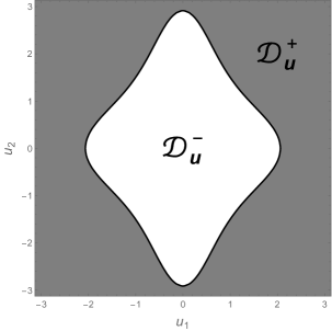
Figure 1: In the gray $\mathcal{D}_{\mathbf{u}}^{+}$ region the discriminant $\Delta(u_{1},u_{2})$ (7.20) is positive and therefore blowups are possible. In the complementary region $\mathcal{D}_{\mathbf{u}}^{-}$ the discriminant $\Delta(u_{1},u_{2})$ is negative and therefore no blowups are possible.

The blowup surface $\Gamma$ has two branches

$$t_{\pm}=\frac{1}{6}\left(4u_{1}^{2}+5u_{2}^{2}\pm\sqrt{4u_{1}^{4}+28u_{2}^{2}u_{1}^{2}+u_{2}^{4}-72}\right)\,.$$ (7.22)

with ${\mathbf{u}}\in\mathcal{D}_{\mathbf{u}}^{+}$. It is easy to see that for both branches $t_{+}\geq t_{-}>0$ (see figure (2)).

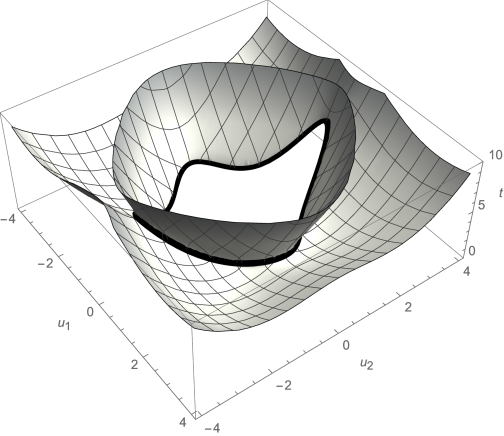
Figure 2: Blowup $\Gamma$ region (7.22) related to hodograph mappings (7.16). At the black curve (7.25) the vorticity behavior is nongeneric $\omega\sim(\Delta t)^{-2}$

The time of the gradient catastrophe is ${t_{-}}_{\mathrm{min}}=1.62019$ at the point $u_{1}=\pm 1.59562$ , $u_{2}=\pm 1.17844$.

The vorticity is equal to

$$\omega_{3}=\frac{3-\frac{2}{3}u_{1}u_{2}}{\det M}\,.$$ (7.23)

In the first regime of approaching of generic blowup point $(u_{1},u_{2})\in\mathcal{D}^{+}_{\mathbf{u}}$ the vorticity behaves as

$$\omega_{3}(t,{\mathbf{u}}_{b})\sim\pm\frac{2u_{1}u_{2}-9}{\sqrt{4u_{1}^{4}+28u_{2}^{2}u_{1}^{2}+u_{2}^{4}-72}\left(t-t_{b}\right)}\,,\qquad t\to t_{b}=\frac{1}{6}\left(4u_{1}^{2}-5u_{2}^{2}\pm\sqrt{4u_{1}^{4}+28u_{2}^{2}u_{1}^{2}+u_{2}^{4}-72}\right)\,.$$ (7.24)

Approaching the points

$${t_{\pm}}_{b}=\frac{2}{3}u_{1}^{2}+\frac{5}{6}u_{2}^{2}\,,\qquad\Delta(u_{1},u_{2})=0\,,$$ (7.25)

which belongs to the curve of intersection of two branches $t_{+}$ and $t_{-}$, the vorticity blows up as

$$\omega\sim\,\frac{\pm\frac{2}{3}\sqrt{2}u_{1}\sqrt{-7u_{1}^{2}-\sqrt{6}\sqrt{8u_{1}^{4}+3}}-3}{\left(t-t_{b}\right)^{2}}\,,\qquad t\to t_{b}=-11u_{1}^{2}-5\sqrt{\frac{16u_{1}^{4}}{3}+2}\,.$$ (7.26)

In this case the curve $\Delta(u_{1},u_{2})=0$ is the boundary line between the subdomains $\mathcal{D}_{\mathbf{u}}^{+}$ and $\mathcal{D}_{\mathbf{u}}^{-}$.

7.3 Gaussian initial data

Finally we consider solution of the HEE with the initial data

$$u_{1}({\mathbf{x}},0)=e^{-x_{1}^{2}-x_{2}^{2}}\,,\qquad u_{2}({\mathbf{x}},0)=\exp^{-x_{1}^{2}-3x_{2}^{2}}\,.$$ (7.27)

Such initial values admits four different open sets of invertibility shown in the table 1.

$$\begin{array}[]{|c|c|c|c|c|}\hline\cr&\begin{array}[]{c}{x_{1}\geq 0\vspace{.1cm}}\\ {x_{2}\geq 0}\end{array}&\begin{array}[]{c}{x_{1}\geq 0\vspace{.1cm}}\\ {x_{2}<0}\end{array}&\begin{array}[]{c}{x_{1}<0\vspace{.1cm}}\\ {x_{2}\geq 0}\end{array}&\begin{array}[]{c}{x_{1}<0\vspace{.1cm}}\\ {x_{2}<0}\end{array}\\ \hline\cr&&&&\\ x_{1}=f_{1}({\mathbf{u}})&\sqrt{\frac{1}{2}\log\frac{u_{2}}{{u_{1}}^{3}}}&\sqrt{\frac{1}{2}\log\frac{u_{2}}{{u_{1}}^{3}}}&-\sqrt{\frac{1}{2}\log\frac{u_{2}}{{u_{1}}^{3}}}&-\sqrt{\frac{1}{2}\log\frac{u_{2}}{{u_{1}}^{3}}}\\ &&&&\\ \hline\cr&&&&\\ x_{2}=f_{2}({\mathbf{u}})&\sqrt{\frac{1}{2}\log\frac{u_{1}}{{u_{2}}}}&-\sqrt{\frac{1}{2}\log\frac{u_{1}}{{u_{2}}}}&\sqrt{\frac{1}{2}\log\frac{u_{1}}{{u_{2}}}}&-\sqrt{\frac{1}{2}\log\frac{u_{1}}{{u_{2}}}}\\ &&&&\\ \hline\cr\end{array}$$

Table 1: The local inverses of the initial data (7.27).

where $f_{i}$, $i=1,2$ is the local inverse of (7.27). The hodograph equations (2.1) assume the form of the system of four equations

$$G_{a,b}:\left\{\begin{array}[]{cc}x_{1}=u_{1}t+a\sqrt{\frac{1}{2}\ln\left(\frac{u_{2}}{u_{1}^{3}}\right)}\,,&a(x_{1}-u_{1}t)>0\\ x_{2}=u_{2}t+b\sqrt{\frac{1}{2}\ln\left(\frac{u_{2}}{u_{1}}\right)}\,,&b(x_{2}-u_{2}t)>0\\ \end{array}\right.\,,\qquad a=\pm\,,b=\pm\,.$$ (7.28)

Each pair of equations (7.28) define a solution ${\mathbf{u}}_{ab}({\mathbf{x}},t)$ in the corresponding subdomain. So, solution of the 2D HEE with the initial data (7.27) is a union

$${\mathbf{u}}({\mathbf{x}},t)={\mathbf{u}}_{++}({\mathbf{x}},t)\cup{\mathbf{u}}_{+-}({\mathbf{x}},t)\cup{\mathbf{u}}_{-+}({\mathbf{x}},t)\cup{\mathbf{u}}_{--}({\mathbf{x}},t)\,.$$ (7.29)

In other words

$${\mathbf{u}}({\mathbf{x}},t)=\left\{\begin{array}[]{c}{\mathbf{u}}_{++}({\mathbf{x}},t)\,,\qquad\mathrm{at}\quad x_{1}-u_{1}({\mathbf{x}},t)>0\,,\quad x_{2}-u_{2}({\mathbf{x}},t)>0\,,\\ {\mathbf{u}}_{+-}({\mathbf{x}},t)\,,\qquad\mathrm{at}\quad x_{1}-u_{1}({\mathbf{x}},t)>0\,,\quad x_{2}-u_{2}({\mathbf{x}},t)<0\,,\\ {\mathbf{u}}_{-+}({\mathbf{x}},t)\,,\qquad\mathrm{at}\quad x_{1}-u_{1}({\mathbf{x}},t)<0\,,\quad x_{2}-u_{2}({\mathbf{x}},t)>0\,,\\ {\mathbf{u}}_{--}({\mathbf{x}},t)\,,\qquad\mathrm{at}\quad x_{1}-u_{1}({\mathbf{x}},t)<0\,,\quad x_{2}-u_{2}({\mathbf{x}},t)<0\,.\end{array}\right.$$ (7.30)

The function (7.30) is continuous on $\mathbb{R}^{2}\times\mathbb{R}$ through the boundary ${\mathbf{x}}-{\mathbf{u}}t=0$. Note that ${\mathbf{u}}_{--}({\mathbf{x}},t)={\mathbf{u}}_{++}(-{\mathbf{x}},-t)$, ${\mathbf{u}}_{-+}({\mathbf{x}},t)={\mathbf{u}}_{+-}(-{\mathbf{x}},-t)$. Moreover the domain $\mathcal{D}_{\mathbf{u}}$ is the square $0<u_{1}({\mathbf{x}},t),u_{2}({\mathbf{x}},t)\leq 1$. Using the standard formulae ${\mathbf{u}}(x,t)={\mathbf{u}}_{0}(\xi_{1},\xi_{2})$ with $\xi_{i}=x_{i}-u_{i}t$, $i=1,2$, one can view the piecewise solution (7.30) as

$$\begin{split}{\mathbf{u}}_{ab}(x,t)={\mathbf{u}}_{0}(a\xi_{1},b\xi_{2})\,,\qquad a\xi_{1}>0\,,\quad b\xi_{2}>0\,.\end{split}$$ (7.31)

Then four corresponding matrices $M$ are of the form

$$M^{(ab)}(t,{\mathbf{u}})=\left(\begin{array}[]{ccc}t-a\frac{3}{2\sqrt{2}{u_{1}}\sqrt{\log\left(\frac{{u_{2}}}{{u_{1}}^{3}}\right)}}&&a\frac{1}{2\sqrt{2}{u_{2}}\sqrt{\log\left(\frac{{u_{2}}}{{u_{1}}^{3}}\right)}}\\ &&\\ b\frac{1}{2\sqrt{2}{u_{1}}\sqrt{\log\left(\frac{{u_{1}}}{{u_{2}}}\right)}}&&t-b\frac{1}{2\sqrt{2}{u_{2}}\sqrt{\log\left(\frac{{u_{1}}}{{u_{2}}}\right)}}\\ \end{array}\right)\,,\qquad a,b=\pm$$ (7.32)

and the corresponding branches of the blowup surface are defined by the equation

$$\det M=t^{2}-\left(\frac{3a}{2\sqrt{2}{u_{1}}\sqrt{\log\left(\frac{{u_{2}}}{{u_{1}}^{3}}\right)}}+\frac{b}{2\sqrt{2}{u_{2}}\sqrt{\log\left(\frac{{u_{1}}}{{u_{2}}}\right)}}\right)t+\frac{ab}{4{u_{1}u_{2}}\sqrt{\log\left(\frac{{u_{2}}}{{u_{1}}^{3}}\right)\log\left(\frac{{u_{1}}}{{u_{2}}}\right)}}=0\,,\quad a,b=\pm\,.$$ (7.33)

The values of the vorticity $\omega_{3}$ for the branches $(a,b)$ are given by

$$\omega_{3}=\frac{1}{\det M_{pq}(t,{\mathbf{u}})}\left(\frac{a}{2\sqrt{2}{u_{2}}\sqrt{\log\left(\frac{{u_{1}}}{{u_{2}}^{3}}\right)}}-\frac{b}{2\sqrt{2}{u_{1}}\sqrt{\log\left(\frac{{u_{2}}}{{u_{1}}}\right)}}\right)\,.$$ (7.34)

The discriminant $\Delta$ of the equation (7.33) is positive for all values of $a$ and $b$ since

$$\begin{split}\Delta_{ab}({\mathbf{u}})=&\left(\frac{3a}{2\sqrt{2}{u_{1}}\sqrt{\log\left(\frac{{u_{2}}}{{u_{1}}^{3}}\right)}}+\frac{b}{2\sqrt{2}{u_{2}}\sqrt{\log\left(\frac{{u_{1}}}{{u_{2}}}\right)}}\right)^{2}-\frac{ab}{{u_{1}u_{2}}\sqrt{\log\left(\frac{{u_{2}}}{{u_{1}}^{3}}\right)\log\left(\frac{{u_{1}}}{{u_{2}}}\right)}}\\ =&\left(\frac{3a}{2\sqrt{2}{u_{1}}\sqrt{\log\left(\frac{{u_{2}}}{{u_{1}}^{3}}\right)}}-\frac{b}{2\sqrt{2}{u_{2}}\sqrt{\log\left(\frac{{u_{1}}}{{u_{2}}}\right)}}\right)^{2}+\frac{ab}{{2u_{1}u_{2}}\sqrt{\log\left(\frac{{u_{2}}}{{u_{1}}^{3}}\right)\log\left(\frac{{u_{1}}}{{u_{2}}}\right)}}\,.\end{split}$$ (7.35)

So, for the solution (7.30) the blowup surface $\Gamma$ has two brances for all values of ${\mathbf{u}}\in\mathcal{D}_{\mathbf{u}}$

$$(t_{\pm})_{ab}=\frac{3a}{2\sqrt{2}{u_{1}}\sqrt{\log\left(\frac{{u_{2}}}{{u_{1}}^{3}}\right)}}+\frac{b}{2\sqrt{2}{u_{2}}\sqrt{\log\left(\frac{{u_{1}}}{{u_{2}}}\right)}}\pm\sqrt{\Delta_{ab}}\,.$$ (7.36)

It is easy to see that for the $(a,b)=(+,+)$ piece

$$(t_{\pm})_{++}>0\,,\qquad(t_{+})_{++}>(t_{-})_{++}\,,$$ (7.37)

while

$$(t_{\pm})_{--}<0\,,\qquad(t_{+})_{--}>(t_{-})_{--}\,,$$ (7.38)

For the pieces $(a,b)=(+,-)$ and $(a,b)=(-,+)$ one has

$$(t_{+})_{+-}>0\,,\qquad(t_{-})_{+-}<0\,,$$ (7.39)

and

$$(t_{+})_{-+}>0\,,\qquad(t_{-})_{-+}<0\,.$$ (7.40)

Minimal values of ${t_{\pm}}_{ab}$ for the positive pieces are

$$(t_{-})_{++}\big{|}_{\min}=0.642593\,,\qquad(t_{+})_{+-}\big{|}_{\min}=1.16582\,,\qquad(t_{+})_{-+}\big{|}_{\min}=0.673088\,.$$ (7.41)

Thus, the gradient catastrophe occurs at

$$t_{c}\equiv(t_{-})_{++}\big{|}_{\min}=0.642593\,,\qquad{\mathbf{u}}_{c}=(0.803494,0.584021)\,,\qquad{\mathbf{x}}_{c}=(0.759774,0.77468)\,.$$ (7.42)

As expected the behavior of the vorticity at ${\mathbf{u}}={\mathbf{u}}_{c}$ in the first regime is

$$\omega(t,{\mathbf{u}}_{c})=\frac{0.270466}{t_{c}-t}-0.0747002+0.0206315(t_{c}-t)+\dots\,.$$ (7.43)

The time evolution of the vorticity $\omega(t,{\mathbf{u}})$ is shown in figure 3.

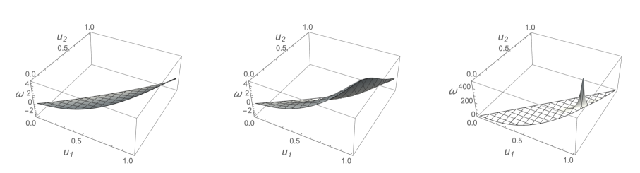
Figure 3: The time evolution of the vorticity depending on ${\mathbf{u}}$ with initial data given by (7.27). From left to right the times are $t=0$, $t=0.85t_{c}$, $t=0.999t_{c}$ where $t_{c}=0.642593$ is the catastrophe time. Remark the change in the vertical scale in the last plot.

In figure 4 it is shown the time evolution of the vorticity w.r.t. to space variables, numerically computed using Mathematica. The behavior is in agreement with the analytical predictions (7.42).

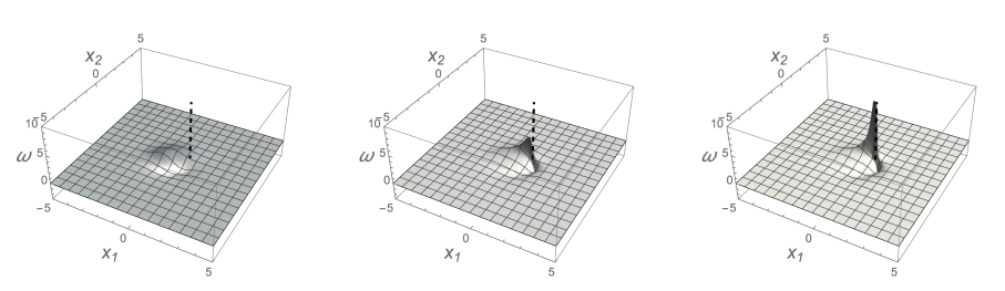
Figure 4: The time evolution of the vorticity depending on ${\mathbf{x}}$ with initial data given by (7.27). From left to right the times are $t=0$, $t=0.85t_{c}$, $t=0.999t_{c}$ where $t_{c}=0.642593$ is the catastrophe time. The dashed vertical line indicates the catastrophe direction of the vorticity in the catastrophe place ${\mathbf{x}}_{c}$.

Since $\Delta_{ab}({\mathbf{u}})\neq 0$ for all ${\mathbf{u}}\in\mathcal{D}_{\mathbf{u}}$, two branches (7.36) do not intersect. So, the blowup of the type $\omega\sim(t_{c}-t)^{-2}$ is absent in this case.

8 Blowups for n-dimensional case.

An extension of the results presented in this paper to the $n$-dimensional HEE is quite straightforward. Indeed, the components $\omega_{ij}$ of the vorticity two-form (4.1) in Cartesian coordinates are given by

$$\omega_{ij}(t,{\mathbf{u}})=(M^{-1})_{ji}(t,{\mathbf{u}})-(M^{-1})_{ij}(t,{\mathbf{u}})=\frac{\widetilde{M}_{ji}(t,{\mathbf{u}})-\widetilde{M}_{ij}(t,{\mathbf{u}})}{\det(M(t,{\mathbf{u}}))}\,,\qquad i,j=1,\dots,n.$$ (8.1)

In the $n$-dimensional case $\det(M(t,{\mathbf{u}}))$ is a polynomial in $t$ of degree $n$ [10], i.e.

$$\det(M(t,{\mathbf{u}}))=\prod_{k=1}^{n}(t-{t_{b}}_{k})\,.$$ (8.2)

So, in the first regime of approaching the blowup point $\omega_{ij}$ may have the following behavior

$$\omega_{ij}\sim(t-t_{b})^{-m}\,,\qquad t\to t_{b}\,,\quad m=1,\dots,n\,.$$ (8.3)

As far as the second regime is concerned it was shown in [11] that the derivatives $\partial u_{i}/\partial x_{j}$ may have singularities of the type $|\delta{\mathbf{x}}|^{-\frac{m}{m+1}}$, with $m=1,\dots,n+1$. Hence, in this regime the vorticity two-form may blow up as

$$\omega_{ij}\sim|\delta{\mathbf{x}}|^{-\frac{m}{m+1}}\,,\qquad|\delta{\mathbf{x}}|\to 0\,,\qquad m=1,\dots,n+1\,.$$ (8.4)

Similar to the results described in [11] blowups of the vorticity exhibit rather rich fine structure.

The formulae (8.3) and (8.4) imply certain behavior of the characteristics of vorticity in different dimensions discussed in [1].

One obtains analogous results for the stress tensor

$$\mathcal{S}_{ij}\equiv\frac{\partial u_{i}}{\partial x_{j}}+\frac{\partial u_{j}}{\partial x_{i}}=(M^{-1})_{ij}+(M^{-1})_{ji}=\frac{\widetilde{M}_{ij}+\widetilde{M}_{ji}}{\det(M)}\,,\qquad i,j=1,\dots,n$$ (8.5)

which is another important quantity in the theory of continuous media [18, 20, 2].

9 Conclusions

The results presented in this note are in part the consequences of those obtained in the paper [11]. As in [11] we are dealing with the most simplified version of the Navier-Stokes equation, namely with HEE (1.1) and do not discuss the possibility of blowups of vorticity of type (1.3) for positive values of time.

All that indicates at least two possible direction of further study. The first is the verification of the realisability of hierarchy of blowups (1.3) for positive times that is of most interest in physical applications.

An extension of such type of analysis for more physical systems would be the second direction. In particular, it may be applicable to those hydrodynamical systems which are obtainable as the constraints of the multidimensional homogeneous Euler equation [9].

Acknowledgments

This project has received funding from the European Union’s Horizon 2020 research and innovation programme under the Marie Skłodowska-Curie grant no 778010 IPaDEGAN. We also gratefully acknowledge the auspices of the GNFM Section of INdAM, under which part of this work was carried out, and the financial support of the project MMNLP (Mathematical Methods in Non Linear Physics) of the INFN.

References

- [1] V. I. Arnold and B. A. Khesin Topological methods in hydrodynamics Springer-Verlag NY (1998)
- [2] G.K. Bachelor An introduction to Fluid Mechanics Cambridge University Press (1970)
- [3] S. G. Chefranov An exact statistical closed description of vortex turbulence and of the diffusion of an impurity in a compressible medium Sov. Phys. Dokl. 36(4) 286-289 (1991)
- [4] S.G. Chefranov and A.S. Chefranov Exact Time-Dependent Solution to the Three-Dimensional Euler- Helmholtz and Riemann-Hopf Equations for Vortex Flow of a Compressible Medium and the Sixth Millennium Prize Problem Phys. Scr. 94 054001 (2019)
- [5] P. Constantin and C. Fefferman Direction of Vorticity and the Problem of Global Regularity for the Navier-Stokes Equations Ind. Univ. Math. J. 42 775-789 (1993)
- [6] P. Constantin, P. D. Lax, and A. Majda A simple one-dimensional model for the three-dimensional vorticity equation Comm. Pure Appl. Math. 38-6 715–724 (1985)
- [7] D.B. Fairlie, Equations of Hydrodynamic Type DTP/93/31(1993)
- [8] E. A. Karabut and E. N. Zhuravleva Unsteady flows with a zero acceleration on the free boundary J. Fluid Mech. 754 308-331 (2014)
- [9] B. G. Konopelchenko and G. Ortenzi On universality of homogeneous Euler equation J. Phys. A: Math. Theor. 54, 204701 (2021)
- [10] B. G. Konopelchenko and G. Ortenzi Homogeneous Euler equation: blowups, gradient catastrophes and singularity of mappings J. Phys. A: Math. Theor. 55, 035203 (2022)
- [11] B. G. Konopelchenko and G. Ortenzi On the fine structure and hierarchy of gradient catastrophes for multidimensional homogeneous Euler equation, https://doi.org/10.48550/arXiv.2210.03939
- [12] E. A. Kuznetsov, M. D. Spector, and V. E. Zakharov Formation of singularities on the free surface of an ideal fluid Phys. Rev. E 49, 1283 (1994)
- [13] E. A. Kuznetsov and V. P. Ruban Hamiltonian dynamics of vortex lines in hydrodynamic type systems JETP Lett. 67, 1076–1081 (1998)
- [14] E. A. Kuznetsov and V. P. Ruban Collapse of vortex lines in hydrodynamics JETP 91, pages 775–785 (2000)
- [15] E. A. Kuznetsov Vortex line representation for flows of ideal and viscous fluids JETP Lett. 76:6, 346–350 (2002)
- [16] E. A. Kuznetsov Towards a sufficient criterion for collapse in 3D Euler equations Physica D 184 266-275 (2003)
- [17] E.A.Kuznetsov and E.A.Mikhailov Slipping flows and their breaking Ann. Phys. in press (2022)
- [18] H. Lamb Hydrodynamics Cambridge University Press (1993)
- [19] A. Majda and A. Bertozzi Vorticity and Incompressible Flow Cambridge University Press (2010)
- [20] L. D. Landau and E. M. Lifshitz Fluid Mechanics Pergamon press (1987)
- [21] P.G. Saffman Vortex Dynamics Cambridge University Press (1992)
- [22] T. Tao Finite time blowup for Lagrangian modifications of the three-dimensional Euler equation Ann. PDE 2 1–79 (2016)
- [23] Y. B. Zel’dovich Gravitational instability: An approximate theory for large density perturbations. Astron. and Astrophys., 5 84-89 (1970)
- [24] N. M. Zubarev and E. A. Karabut Exact local solutions for the formation of singularities on the free surface of an ideal fluid JETP Lett.107 412-417 (2018)