The ADMM-PINNs Algorithmic Framework for Nonsmooth PDE-Constrained Optimization: A Deep Learning Approach

Abstract.

We study the combination of the alternating direction method of multipliers (ADMM) with physics-informed neural networks (PINNs) for a general class of nonsmooth partial differential equation (PDE)-constrained optimization problems, where additional regularization can be employed for constraints on the control or design variables. The resulting ADMM-PINNs algorithmic framework substantially enlarges the applicable range of PINNs to nonsmooth cases of PDE-constrained optimization problems. The application of the ADMM makes it possible to untie the PDE constraints and the nonsmooth regularization terms for iterations. Accordingly, at each iteration, one of the resulting subproblems is a smooth PDE-constrained optimization which can be efficiently solved by PINNs, and the other is a simple nonsmooth optimization problem which usually has a closed-form solution or can be efficiently solved by various standard optimization algorithms or pre-trained neural networks. The ADMM-PINNs algorithmic framework does not require to solve PDEs repeatedly, and it is mesh-free, easy to implement, and scalable to different PDE settings. We validate the efficiency of the ADMM-PINNs algorithmic framework by different prototype applications, including inverse potential problems, source identification in elliptic equations, control constrained optimal control of the Burgers equation, and sparse optimal control of parabolic equations.

1. Introduction

Partial differential equations (PDEs) are fundamental mathematical tools for studying complex systems in physics, engineering, mechanics, chemistry, finance, and others. In addition to modelling and simulating such a system, it is very often to consider how to optimize or control such a system with certain goals. Hence, PDE-constrained optimization problems arise widely in various areas such as optimal control [33, 43, 64], inverse problems [5, 39], shape design [42], just to mention a few. In practice, additional constraints are always imposed on the control (or design, depending on the application) variables to ensure some desired properties, such as boundedness, sparsity, and discontinuity (see e.g., [12, 43, 57, 64]). Considerations of these additional constraints hence immediately result in nonsmooth PDE-constrained optimization problems. Solving such a nonsmooth PDE-constrained optimization problem is generally even more challenging due to the coupling of PDE constraints with the additional constraints on the control (or design) variables. Moreover, the nonsmoothness feature prevents straightforward applications of some canonical algorithms such as gradient type methods. These difficulties, together with other intrinsic difficulties such as the curse of high dimensionality and ill-conditioning of the resulting algebraic systems after mesh-based numerical discretization, make extremely difficult solving such a nonsmooth PDE-constrained optimization problem. Meticulous techniques for algorithm design are thus needed, and usually the structure and features of the problem under consideration should be well considered to design application-tailored algorithms for a specific application.

1.1. Model

A general class of nonsmooth PDE-constrained optimization problems can be mathematically expressed as

(1.1) $$\min_{y\in Y,u\in U}{J}(y,u)+R(u)\qquad\text{s.t.}~{}e(y,u)=0,$$

where $Y$ and $U$ are Banach spaces; the operator $e:Y\times U\rightarrow Z$ with $Z$ a Banach space, and $e(y,u)=0$ represents a PDE or a system of coupled PDEs defining on $\bar{\Omega}=\Omega\cup\partial\Omega$ with $\Omega\subset\mathbb{R}^{d}(d\geq 1)$ a bounded domain and $\partial\Omega$ its boundary. Throughout, we assume that $e(y,u)=0$ is well posed. That is, for any given $u\in U$, it admits a unique corresponding solution $y(u)\in Y$. Above, $u$ and $y$ are called the control/design variable and the state variable, respectively. The functional $J:Y\times U\rightarrow\mathbb{R}$ consists of a data-fidelity term and a possible smooth regularization. The nonsmooth functional $R:U\rightarrow\mathbb{R}$ is employed to capture some prior information on $u$, such as sparsity, discontinuity, and lower and/or upper bounds. The goal of problem (1.1) is to find an unknown function $u$ such that the objective functional $J(y,u)+R(u)$ is (locally) minimized subject to the PDE constraint $e(y,u)=0$.

Various PDE-constrained optimization problems can be covered by (1.1). For instance, the abstract equation $e(y,u)=0$ can be specified as different PDEs, such as parabolic equations [21, 23], elliptic equations [33], hyperbolic equations [22], and fractional diffusion equations [8]. The unknown function $u$ can be a source term, coefficients, boundary or initial value of the PDE $e(y,u)=0$. The nonsmooth term $R(u)$ can be the indicator function of an admissible set or an $L^{1}$-regularization to promote the sparsity of $u$ as studied in [57]. Given a target or observed function $y_{d}$, typical examples covered by problem (1.1) include the following:

• Control constrained optimal control problems [33, 43, 64]: $J(y,u)=\frac{1}{2}\|y-y_{d}\|^{2}+\frac{\alpha}{2}\|u\|^{2}$ and $R(u)=I_{U_{ad}}(u)$ with $\alpha>0$. Here, $I_{U_{ad}}:U\rightarrow\mathbb{R}\cup\{\infty\}$ is the indicator function of the set $U_{ad}$ given by $I_{U_{ad}}(u)=0$ if $u\in U_{ad}$, and $I_{U_{ad}}(u)=+\infty$ otherwise. The set $U_{ad}$ can be a pointwise control set $U_{ad}=\{u\in U,|a\leq u(x)\leq b~{}\text{a.e.~{}in}~{}\Omega\}$ or an integral control set $U_{ad}=\{u\in U,|a\leq\int_{\Omega}udx\leq b\}$ with $a$ and $b$ two constants. The term $R(u)$ imposes additional bounded constraints on the variable $u$.

• Sparse optimal control problems [7, 56, 57]: $J(y,u)=\frac{1}{2}\|y-y_{d}\|^{2}+\frac{\alpha}{2}\|u\|^{2}$ and $R(u)=\rho\|u\|_{L^{1}(\Omega)}$ with $\alpha>0$ and $\rho>0$. The $L^{1}$-regularization $R(u)$ promotes the variable $u$ to be sparse [57] and captures important applications in various fields such as optimal actuator placement [57] and impulse control [15].

• Discontinuous parameter or source identification [12, 13]: $J(y,u)=\frac{1}{2}\|y-y_{d}\|^{2}$ and $R(u)=\gamma\int_{\Omega}|\nabla u|dx$ with $\gamma>0$ a total variation (TV) regularization. The TV-regularization $R(u)$ is capable of reserving the piecewise-constant property of $u$ and has found various applications such as image denoising and electrical impedance tomography.

1.2. Traditional Numerical Approaches

In the literature, there are some numerical approaches for solving some specific cases of (1.1), and these approaches primarily focused on developing iterative schemes that can overcome the difficulty of the nonsmoothness of the underlying objective functional. For instance, the semismooth Newton (SSN) methods [18, 33], the inexact Uzawa method [59], and the alternating direction method of multipliers (ADMM) [26] have been studied for various control constrained optimal control problems. The SSN method [57], the primal-dual algorithm [7], and the proximal gradient method [56] have been respectively proposed for solving sparse optimal control problems. The augmented Lagrangian methods [12, 13] and the ADMM [63] have been applied to parameter identification problems. These approaches are based on the so-called adjoint methodology, which provides an efficient way to compute gradients. However, adjoint-based iterative schemes suffer from high computational costs because the PDEs and their adjoint systems are required to be solved repeatedly. These PDEs are usually solved by mesh-based numerical discretization schemes (e.g., finite difference method (FDM) or finite element method (FEM)), which require solving large-scale and ill-conditioned systems. As a single call to the underlying PDE solver can be very expensive, computing the PDEs and their adjoint systems repeatedly could be prohibitively expensive in practice.

1.3. Physics-Informed Neural Networks

Deep learning has recently emerged as a new powerful tool for scientific computing thanks to the universal approximation property [17] and great expressibility of deep neural networks (DNNs) [53]. In particular, deep learning approaches have been used for PDE-related problems, see e.g., [6, 16, 19, 27, 35, 37, 44, 54, 58, 70, 75] and references therein. Among them, Physics-Informed Neural Networks (PINNs), which can date back to the 1990s [41, 52] and were phenomenally popularized by [54] and others, have been extensively studied for various PDEs. In principle, PINNs approximate the unknowns by neural networks and minimize a loss function that includes the residuals of the PDEs and initial and boundary conditions. The loss is evaluated at a set of scattered spatial-temporal points and the PDEs are solved when the loss goes to zero. In general, PINNs are mesh-free, easy-to-implement, and flexible to different PDEs. We refer to the review papers [16, 20, 28, 35, 44] and references therein for more discussions.

It has been shown in [48, 54] that PINNs can be easily extended to PDE-constrained optimization problems by approximating the control or design variable with another neural network in addition to the one for the unknown state variable. Then, these two neural networks can be simultaneously trained using a composite loss function consisting of the objective functional and the residuals of the PDE constraint. In this way, the training process finds a solution that satisfies the PDE constraint while minimizing the objective functional. Moreover, it is worth noting that PINNs are very flexible in terms of the type of PDE, initial/boundary conditions, geometries of the domain, and objective functionals. Hence, PINNs can be easily adapted to solve a large class of PDE-constrained optimization with little human effort in algorithmic design. In this regard, PINNs have been successfully applied to solve optimal control problems [48], inverse problems [54], and shape design [61], just to name a few. In addition to such direct extensions of PINNs, the Control PINN [3] solves PDE-constrained optimization by deriving the first-order optimality conditions, and then approximating the control/design variable, the state variable, and the adjoint variable by different DNNs, respectively. Then, a stationary point of the PDE-constrained optimization can be computed by minimizing a loss function that consists of the residuals of the first-order optimality conditions. In [29], a bi-level PINNs framework is proposed for solving PDE-constrained optimization problems, where the lower-level optimization problem corresponds to the PDE constraints and the upper-level optimization problem finds a control variable for minimizing the objective functional. In this way, minimizing the objective functional and solving the PDE constraint are decoupled; and the challenge of tuning the weights in the loss function of the standard PINNs is addressed.

In the above-mentioned PINNs-based methods, the underlying PDE and initial/boundary conditions are penalized in the loss function with constant penalty parameters. Hence, the PDE is treated as a soft constraint and the obtained solution may not satisfy the PDE constraint and thus is not a valid solution. To address this issue, some hybrid numerical PDE-PINNs are proposed, see e.g., [47, 50, 71], which combine classical PDE solvers with neural networks, for solving PDE-constrained optimization problems. These approaches train the embedded neural networks while numerically satisfying the PDE constraint. In [71], inverse problems of PDEs are considered, which aim at identifying unknown parameters in the PDEs from some available observation data. For solving such problems, a physics constrained learning approach is proposed, which represents the unknown parameters by neural networks and trains the embedded DNNs while the PDE constraint is solved by traditional numerical solvers. A hybrid FEM-NN approach is proposed in [47] to recover coefficients and missing PDE operators from observations, in which the unknowns are represented by neural networks and the PDE is discretized by a finite element method.

Alternative to the hybrid numerical PDE-PINNs, one can also consider combining optimization algorithms with PINNs, and thus develop some hybrid optimization-PINNs to impose hard constraints. To this end, one can consider applying the augmented Lagrangian method (ALM) [30, 51], which is known to be more efficient than penalty methods. For instance, a physics and equality constrained artificial neural network is proposed in [4] for inverse problems, where the ALM is employed to enforce the initial/boundary conditions of the PDEs and any other possible high-fidelity data. In [45], PINNs with hard constraints (hPINNs) are proposed for solving PDE-constrained optimization originating from inverse design. The hPINNs treat the PDE and additional inequality constraints as hard constraints by using the ALM.

1.4. Motivation and Our Numerical Approach

Compared with traditional iterative methods which discretize the involved PDEs, PINNs-based methods are usually mesh-free, easy to implement, and flexible to different PDEs. Moreover, PINNs-based methods avoid solving adjoint systems completely by taking advantage of automatic differentiation, and could break the curse of dimensionality; computational costs can thus be reduced substantially. Despite these advantages, it is worth noting that all the above-mentioned PINNs methods (except [45]) solved only smooth PDE-constrained optimization and they cannot be directly applied to generic nonsmooth problems like (1.1). A particular reason is that when the variable $u$ is approximated by a neural network $\mathcal{NN}_{u}$, the term $R(\mathcal{NN}_{u})$ appears in the loss function. From a rigorous mathematical point of view, the nonsmoothness of $R(\mathcal{NN}_{u})$ prevents the application of commonly used neural network training technologies (e.g., back-propagation and stochastic gradient methods), which makes the neural network unfeasible to be trained. The same concern also applies to other recently developed deep learning algorithms for solving PDE-constrained optimization, such as the ISMO [46], the operator learning methods [34, 68], and the amortized finite element analysis [73]. The ALM-based PINN in [45] can treat inequality constraints but it does not apply to other nonsmooth cases like $R(u)=\|u\|_{L^{1}(\Omega)}$ and $R(u)=\int_{\Omega}|\nabla u|dx$ in (1.1). To our best knowledge, there seems no deep learning approach in the literature that can tackle the generic nonsmooth PDE-constrained optimization model (1.1). Hence, it is of our interest to develop new deep learning approaches for solving (1.1) by exploring its specific mathematical structure.

Motivated by the aforementioned nice properties and the popularity of PINNs, we develop a PINNs algorithmic framework for solving (1.1). Recall that applying PINNs directly to solve (1.1) is not available. To bypass this issue, our philosophy is that the structures and properties of the model should be sophisticatedly considered in algorithmic design. One particular goal is to untie the PDE constraint $e(y,u)=0$ and the nonsmooth regularization $R(u)$ so that these two inherently different terms can be treated individually. To this end, we consider the ADMM, which is a representative operator splitting method introduced by Glowinski and Marroco in [24] for nonlinear elliptic problems. The ADMM can be regarded as a splitting version of the ALM, where the subproblem is decomposed into two parts and they are solved in the Gauss-Seidel manner. A key feature of the ADMM is that the decomposed subproblems usually are much easier than the ALM subproblems, which makes the ADMM a benchmark algorithm in various areas. In particular, the ADMM has been recently applied to solve some optimal control problems in [25, 26] and inverse problems in [40, 63].

In this paper, we advocate combining the ADMM with PINNs, and propose the ADMM-PINNs algorithmic framework for solving (1.1). The ADMM-PINNs algorithmic framework inherits all the advantages of the ADMM and PINNs. On one hand, as shown in Section 2, the ADMM-PINNs algorithmic framework can treat the PDE constraint $e(y,u)=0$ and the nonsmooth regularization $R(u)$ individually and only needs to solve two simple subproblems. One subproblem is a smooth PDE-constrained optimization problem, which can be efficiently solved by various PINNs. The other one is a simple nonsmooth optimization problem, which usually has a closed-form solution or can be efficiently solved by various well-developed optimization algorithms or pre-trained DNNs. On the other hand, compared with traditional numerical methods with mesh-based discretization as the PDE solvers, the ADMM-PINNs algorithmic framework does not require to solve PDEs repeatedly, and it is mesh-free, easy to implement, and scalable to different settings.

We validate the effectiveness and flexibility of the ADMM-PINNs algorithmic framework through different case studies. In particular, we consider different cases of $e(y,u)=0$ (i.e., different PDEs) and nonsmooth regularization $R(u)$, and implement the ADMM-PINNs algorithmic framework to four prototype applications: inverse potential problem, control constrained optimal control of the Burgers equation, source identification in elliptic equations, and sparse optimal control of parabolic equations. For comparison purposes, we also compare our results with the reference ones obtained by high-fidelity traditional numerical methods based on finite element discretization.

1.5. Organization

The rest of this paper is organized as follows. In Section 2, we present the ADMM-PINNs algorithmic framework and discuss the solutions to the subproblems. Then, to elaborate the implementation of the ADMM-PINNs algorithmic framework, we consider an inverse potential problem in Section 3, control constrained optimal control of the Burgers equation in Section 4, source identification for elliptic equations in Section 5, and sparse optimal control of parabolic equations in Section 6, respectively. Some specific ADMM-PINNs algorithms are derived for solving the above-mentioned concrete applications. The effectiveness and efficiency of the resulting ADMM-PINNs algorithms are demonstrated in each section by some preliminary numerical results. Finally, some conclusions and future perspectives are reported in Section 7.

2. An ADMM-PINNs algorithmic framework

In this section, we first discuss the implementation of ADMM to (1.1) and then take a close look at the application of PINNs to the solutions of the subproblems in each ADMM iteration. An ADMM-PINNs algorithmic framework for solving (1.1) is thus proposed.

2.1. ADMM

For any given $u\in U$, let $y(u)$ be the corresponding solution to the PDE constraint $e(y,u)=0$. Then, problem (1.1) can be rewritten as the following unconstrained optimization problem

(2.1) $$\min_{u\in U}{J}(y(u),u)+R(u).$$

Next, we introduce an auxiliary variable $z\in U$ satisfying $z=u$. Then, problem (2.1) is equivalent to the following linearly constrained separable optimization problem

(2.2) $$\min_{u,z\in U}J(y(u),u)+R(z),\qquad\text{s.t.}\quad u=z.$$

An augmented Lagrangian functional associated with (2.2) can be defined as

$$L_{\beta}(u,z;\lambda)={J}(y(u),u)+R(z)-(\lambda,u-z)+\frac{\beta}{2}\|u-z\|^{2},$$

where $\beta>0$ is a penalty parameter and $\lambda\in U$ is the Lagrange multiplier associated with $u=z$. Here and in what follows, the notations $(\cdot,\cdot)$ and $\|\cdot\|$ stand for the canonical $L^{2}$-inner product and $L^{2}$-norm, respectively. Then, applying the ADMM [24] to (2.2), we readily obtain the following iterative scheme

(2.3a) $$u^{k+1}=\arg\min_{u\in U}L_{\beta}(u,z^{k};\lambda^{k}),$$

(2.3b) $$z^{k+1}=\arg\min_{z\in U}L_{\beta}(u^{k+1},z;\lambda^{k}),$$

(2.3c) $$\lambda^{k+1}=\lambda^{k}-\beta(u^{k+1}-z^{k+1}).$$

It is easy to see that the ADMM decouples the nonsmooth regularization $R(u)$ and the PDE constraint $e(y,u)=0$ at each iteration. We shall show in the rest part of this section that the subproblem (2.3a) can be efficiently solved by PINNs and the subproblem (2.3b) usually has a closed-form solution or can be efficiently solved by some well-developed numerical solvers.

2.2. Solution to the $u$-subproblem (2.3a)

We first note that the $u$-subproblem (2.3a) is equivalent to the following PDE-constrained optimization problem:

(2.4) $$\left\{\begin{aligned} &\min_{y,u}\mathcal{J}^{k}(y,u):=J(y,u)-(\lambda^{k},u-z^{k})+\frac{\beta}{2}\|u-z^{k}\|^{2}\\ &\qquad\text{s.t.}~{}e(y,u)=0.\end{aligned}\right.$$

Next, we specify two PINNs algorithms for solving problem (2.4). The first one is called approximate-then-optimize (AtO) PINNs, where we first approximate problem (2.4) by neural networks and then apply PINNs to solve the resulting problem. The AtO-PINNs can be viewed as a generalization of the classic discretize-then-optimize approach, which first discretizes a PDE-constrained optimization by a certain numerical scheme (e.g., FDM or FEM) to obtain a discrete approximation, and then optimize the problem in the discrete setting. More discussions on the comparison between neural networks approximation and finite element discretization can be found in [44]. The second one is referred to as optimize-then-approximate (OtA) PINNs, which means that we derive the first-order optimality system of (2.4) in continuous settings and then approximate it by neural networks and solve it by PINNs. The OtA-PINNs is a generalization of the classic optimize-then-discretize approach, which discretizes the continuous optimality system by a certain numerical scheme.

2.2.1. An approximate-then-optimize PINNs algorithm

In this subsection, by generalizing the classic discretize-then-optimize approach, we specify an AtO-PINNs algorithm to solve (2.4).

To approximate problem (2.4), we construct two neural networks $\hat{y}(x;\bm{\theta}_{y})$ parameterized by $\bm{\theta}_{y}$ and $\hat{u}(x;\bm{\theta}_{u})$ parameterized by $\bm{\theta}_{u}$ to approximate $y$ and $u$, respectively. We can show that subproblem (2.4) can be approximated by the following optimization problem:

(2.5) $$\left\{\begin{aligned} &\min_{\bm{\theta}_{y},\bm{\theta}_{u}}J(\hat{y}(x;\bm{\theta}_{y}),\hat{u}(x;\bm{\theta}_{u}))-(\lambda^{k}(x),\hat{u}(x;\bm{\theta}_{u})-z^{k}(x))+\frac{\beta}{2}\|\hat{u}(x;\bm{\theta}_{u})-z^{k}(x)\|^{2}\\ &\qquad\text{s.t.}~{}e(\hat{y}(x;\bm{\theta}_{y}),\hat{u}(x;\bm{\theta}_{u}))=0.\end{aligned}\right.$$

We then apply the vanilla PINNs [54] to solve problem (2.5) and the resulting algorithm is listed in Algorithm 1.

Algorithm 1 AtO-PINNs for (2.4)

1:  Input: Initial parameters $\bm{\theta}_{y}^{0},\bm{\theta}_{u}^{0}$ and weights $w_{e}>0,w_{o}>0$

2:  Choose training set $\mathcal{T}=\mathcal{T}_{i}\cup\mathcal{T}_{b}$ with $\mathcal{T}_{i}\subset\Omega$ and $\mathcal{T}_{b}\subset\partial\Omega$.

3:  Train the neural networks to find $\bm{\theta}_{y}^{k+1}$ and $\bm{\theta}_{u}^{k+1}$ by minimizing the following total loss function

(2.6) $$\mathcal{L}_{total}^{k}(\bm{\theta}_{y},\bm{\theta}_{u})=w_{o}\mathcal{J}^{k}(\bm{\theta}_{y},\bm{\theta}_{u})+w_{e}\mathcal{L}_{PDE}(\bm{\theta}_{y},\bm{\theta}_{u}),$$

where

$$\mathcal{J}^{k}(\bm{\theta}_{y},\bm{\theta}_{u}):=\frac{1}{|\mathcal{T}|}\sum_{x\in\mathcal{T}}\left(J(\hat{y}(x;\bm{\theta}_{y}),\hat{u}(x;\bm{\theta}_{u}))-(\lambda^{k}(x),\hat{u}(x;\bm{\theta}_{u})-z^{k}(x))+\frac{\beta}{2}\|\hat{u}(x;\bm{\theta}_{u})-z^{k}(x)\|^{2}\right),$$

and

$$\mathcal{L}_{PDE}(\bm{\theta}_{y},\bm{\theta}_{u})=\frac{1}{|\mathcal{T}|}\sum_{x\in\mathcal{T}}\|e(\hat{y}(x;\bm{\theta}_{y}),\hat{u}(x;\bm{\theta}_{u}))\|^{2}.$$

4:  Output: Parameters $(\bm{\theta}_{y}^{k+1},\bm{\theta}_{u}^{k+1})$ and approximate solutions $\hat{y}(x;\bm{\theta}^{k+1}_{y})$ and $\hat{u}(x;\bm{\theta}^{k+1}_{u})$.

Remark 2.1.

To expose our main ideas clearly, the vanilla PINNs algorithm is employed in Algorithm 1 for solving (2.4). It is worth noting that some other PINNs-based algorithms (e.g., VPINN [36], gPINN [72], and CAN-PINN [14]) can also be applied in a similar way.

In the context of PINNs, the training sets $\mathcal{T}_{i}$ and $\mathcal{T}_{b}$ are usually referred to as the sets of residual points. For the choice of the residual points, there are generally three possible strategies: 1) specify the residual points at the beginning of training, which could be grid points on a lattice or random points, and never change them during the training process; 2) select different residual points randomly in each optimization iteration of the training process; 3) improve the location of the residual points adaptively during the training process, see e.g., [44]. Moreover, we remark that for time-dependent problems, the time variable $t$ can be treated as an additional space coordinate and $\Omega$ denotes the spatial-temporal domain. Then, the initial and boundary conditions can be treated similarly. Note that in Algorithm 1, the calculation of $\mathcal{L}_{total}^{k}(\bm{\theta}_{y},\bm{\theta}_{u})$ usually involves derivatives, such as the partial derivatives $\frac{\partial\hat{y}}{\partial x}$ and $\frac{\partial^{2}\hat{y}}{\partial x^{2}}$, which are handled via automatic differentiation.

Starting from some initialized parameters $\bm{\theta}_{y}^{0}$ and $\bm{\theta}_{u}^{0}$, we use stochastic optimization algorithms to find $\bm{\theta}^{k+1}_{y}$ and $\bm{\theta}_{u}^{k+1}$ that minimize (2.6). For instance, at each inner iteration indexed by $j$, the parameters from both neural networks can concurrently be updated by

$$\bm{\theta}_{y}\leftarrow\bm{\theta}_{y}-\eta_{j}\frac{\partial\mathcal{L}^{k}_{total}}{\partial\bm{\theta}_{y}}(\bm{\theta}_{y},\bm{\theta}_{u}),~{}\text{and}~{}\bm{\theta}_{u}\leftarrow\bm{\theta}_{u}-\eta_{j}\frac{\partial\mathcal{L}^{k}_{total}}{\partial\bm{\theta}_{u}}(\bm{\theta}_{y},\bm{\theta}_{u}),$$

where $\eta_{j}>0$ is an appropriate learning rate. All gradients (i.e. $\frac{\partial\mathcal{L}^{k}_{total}}{\partial\bm{\theta}_{y}}$ and $\frac{\partial\mathcal{L}^{k}_{total}}{\partial\bm{\theta}_{u}}$) are computed using automatic differentiation. At the end of the training process, the trained neural networks $\hat{y}(x;\bm{\theta}_{y}^{k+1})$ and $\hat{u}(x;\bm{\theta}_{u}^{k+1})$ approximately solve problem (2.5).

2.2.2. An optimize-then-approximate PINNs algorithm

In this subsection, we derive an OtA-PINNs algorithm to solve the $u$-subproblem (2.4). A similar idea can also be found in [3].

Following some standard arguments as those in [33], one can show that, if $({y},u)$ is a solution of (2.4), the optimality system of (2.4) reads as:

(2.7) $$\left\{\begin{aligned} e_{u}({y},u)^{*}p+\mathcal{J}^{k}_{u}({y},u)=0,\\ e({y},u)=0,\\ e_{y}({y},u)^{*}p+\mathcal{J}^{k}_{y}({y},u)=0,\end{aligned}\right.$$

where $p$ is the corresponding adjoint variable, $\mathcal{J}_{u}^{k}$ and $\mathcal{J}_{y}^{k}$ are the first-order partial derivatives of $\mathcal{J}^{k}$ with respect to $u$ and $y$, respectively . Then, one can compute a solution $(y,u)$ of problem (2.4) by solving the optimality system (2.7). For this purpose, we construct three neural networks $\hat{y}(x;\bm{\theta}_{y})$ parameterized by $\bm{\theta}_{y}$, $\hat{u}(x;\bm{\theta}_{u})$ parameterized by $\bm{\theta}_{u}$, and $\hat{p}(x;\bm{\theta}_{p})$ parameterized by $\bm{\theta}_{p}$, to approximate $y$, $u$ and $p$, respectively. Then, we approximate the optimality system (2.7) by

(2.8) $$\left\{\begin{aligned} e_{u}(\hat{y}(x;\bm{\theta}_{y}),\hat{u}(x;\bm{\theta}_{u}))^{*}\hat{p}(x;\bm{\theta}_{p})+\mathcal{J}^{k}_{u}(\hat{y}(x;\bm{\theta}_{y}),\hat{u}(x;\bm{\theta}_{u}))=0,\\ e(\hat{y}(x;\bm{\theta}_{y}),\hat{u}(x;\bm{\theta}_{u}))=0,\\ e_{y}(\hat{y}(x;\bm{\theta}_{y}),\hat{u}(x;\bm{\theta}_{u}))^{*}\hat{p}(x;\bm{\theta}_{p})+\mathcal{J}^{k}_{y}(\hat{y}(x;\bm{\theta}_{y}),\hat{u}(x;\bm{\theta}_{u}))=0.\end{aligned}\right.$$

Remark 2.2.

Instead of the full optimality system (2.7), we can also use a reduced optimality system obtained by eliminating $u,y$ or $p$ in (2.7) to implement the OtA-PINNs algorithm. More details are presented in Sections 4 and 6.

A PINNs algorithm for solving (2.8) is presented in Algorithm 2.

Algorithm 2 OtA-PINNs for (2.4)

1:  Input: Initial parameters $\bm{\theta}_{y}^{0},\bm{\theta}_{u}^{0},\bm{\theta}_{p}^{0}$ and weights $w_{u}>0,w_{y}>0,w_{p}>0$.

2:  Choose training sets $\mathcal{T}=\mathcal{T}_{i}\cup\mathcal{T}_{b}$ with $\mathcal{T}_{i}\subset\Omega$ and $\mathcal{T}_{b}\subset\partial\Omega$.

3:  Specify a loss function by summing the weighted $L_{2}$ norm residuals of (2.8).

(2.9) $$\mathcal{L}_{OS}(\bm{\theta}_{y},\bm{\theta}_{u},\bm{\theta}_{p})= \frac{w_{u}}{|\mathcal{T}|}\sum_{x\in\mathcal{T}}\|e_{u}(\hat{y}(x;\bm{\theta}_{y}),\hat{u}(x;\bm{\theta}_{u}))^{*}\hat{p}(x;\bm{\theta}_{p})+\mathcal{J}^{k}_{u}(\hat{y}(x;\bm{\theta}_{y}),\hat{u}(x;\bm{\theta}_{u}))\|^{2}$$

$$+\frac{w_{y}}{|\mathcal{T}|}\sum_{x\in\mathcal{T}}\|e(\hat{y}(x;\bm{\theta}_{y}),\hat{u}(x;\bm{\theta}_{u}))\|^{2}$$

$$+\frac{w_{p}}{|\mathcal{T}|}\sum_{x\in\mathcal{T}}\|e_{y}(\hat{y}(x;\bm{\theta}_{y}),\hat{u}(x;\bm{\theta}_{u}))^{*}\hat{p}(x;\bm{\theta}_{p})+\mathcal{J}^{k}_{y}(\hat{y}(x;\bm{\theta}_{y}),\hat{u}(x;\bm{\theta}_{u}))\|^{2}.$$

4:  Train the neural networks to find $\bm{\theta}_{y}^{k+1}$, $\bm{\theta}_{u}^{k+1}$, and $\bm{\theta}_{p}^{k+1}$ by minimizing (2.9).

5:  Output: Parameters $(\bm{\theta}_{y}^{k+1},\bm{\theta}_{u}^{k+1})$ and approximate solutions $\hat{y}(x;\bm{\theta}^{k+1}_{y})$ and $\hat{u}(x;\bm{\theta}^{k+1}_{u})$.

2.3. Solution to the $z$-subproblem (2.3b)

It can be shown that subproblem (2.3b) is a simple optimization problem corresponding to the nonsmooth term $R(z)$:

(2.10) $$z^{k+1}=\arg\min_{z}R(z)+\frac{\beta}{2}\|z-(u^{k+1}-\frac{\lambda^{k}}{\beta})\|^{2},$$

where $u^{k+1}:=\hat{u}(x;\bm{\theta}_{u}^{k+1})$ is the solution of the $u$-subproblem (2.3a). Problem (2.10) usually has a closed-form solution or can be efficiently solved by some well-developed numerical solvers. For instance,

• if $R(z)=I_{U_{ad}}(z)$ is the indicator function of the set $U_{ad}=\{z\in U,|a\leq z(x)\leq b~{}\text{a.e. in}~{}\Omega\}$ with $a$ and $b$ two constants, then $z^{k+1}(x)=\mathbb{P}_{U_{ad}}\left(u^{k+1}-\frac{\lambda^{k}}{\beta}\right)(x)$, a.e. in $\Omega$, where $\mathbb{P}_{U_{ad}}$ is the projection onto $U_{ad}$ defined by

  $$\mathbb{P}_{U_{ad}}(z)(x):=\max\{\min\{z(x),b\},a\},\text{a.e.~{}in}~{}\Omega.$$

• if $R(z)=\rho\|z\|_{L^{1}(\Omega)}$ is an $L^{1}$-regularization term, then $z^{k+1}(x)=\mathbb{S}_{\frac{\rho}{\beta}}\left(u^{k+1}-\frac{\lambda^{k}}{\beta}\right)(x),$ a.e. in $\Omega$, where $\mathbb{S}$ is the Shrinkage operator defined by

  (2.11) $$\mathbb{S}_{\zeta}(v)(x)=\begin{cases}v(x)-\zeta,&v(x)>\zeta,\\ 0,&|v(x)|\leq\zeta,\\ v(x)+\zeta,&v(x)<-\zeta.\end{cases}$$

• if $R(z)=\gamma\int_{\Omega}|\nabla z|dx$ is a TV-regularization term defined by

  (2.12) $$\int_{\Omega}|\nabla z|dx:=\sup\Big{\{}\int_{\Omega}z~{}\mathrm{div}\varphi~{}\mathrm{d}x:\varphi\in C_{c}^{1}(\Omega;\mathbb{R}^{d}),\|\varphi\|_{\infty}\leq 1\Big{\}},$$

  where $\|\varphi\|_{\infty}=\sup_{x\in\Omega}(\sum_{i=1}^{d}|\varphi_{i}(x)|^{2})^{1/2}$, “div” denotes the divergence operator, and $C_{c}^{1}(\Omega;\mathbb{R}^{d})$ is the set of once continuously differentiable $\mathbb{R}^{d}$-valued functions with compact support in $\Omega$, see, e.g., [76] for more details. In this case, the resulting $z$-subproblem (2.10) has no closed-form solution, but iterative numerical algorithms for solving such a problem have been extensively studied in the literature, such as the split Bregman method [9], the primal-dual method [11], and Chambolle’s dual method [10]. Moreover, when $\Omega\subset\mathbb{R}^{2}$ is a rectangle, the $z$-subproblem (2.10) can be viewed as an image denoising model, which, as shown in [63], can be efficiently solved by some pre-trained deep convolutional neural networks (CNNs), see Section 5 for the details. Here, we present an ADMM algorithm, which is closely related to the split Bregman method [9], to solve problem (2.10). For this purpose, we first reformulate (2.10) as the following constrained optimization problem:

  (2.13) $$\min\gamma\int_{\Omega}|w|dx+\frac{\beta}{2}\|z-(u^{k+1}-\frac{\lambda^{k}}{\beta})\|^{2},~{}\text{s.t.}~{}\nabla z=w.$$

  An augmented Lagrangian functional associated with problem (2.13) is defined as

  $$L_{\zeta}(z,w;\mu)=\gamma\int_{\Omega}|w|dx+\frac{\beta}{2}\|z-(u^{k+1}-\frac{\lambda^{k}}{\beta})\|^{2}-(\mu,\nabla z-w)+\frac{\zeta}{2}\|\nabla z-w\|^{2},$$

  where $\zeta>0$ is a penalty parameter and $\mu$ is the Lagrange multiplier associated with $\nabla z=w$. Then the iterative scheme of ADMM for solving problem (3.5) reads as

  (2.14a) $$z_{j+1}=\arg\min\frac{\beta}{2}\|z-(u^{k+1}-\frac{\lambda^{k}}{\beta})\|^{2}+\frac{\zeta}{2}\|\nabla z-(w_{j}+\frac{\mu_{j}}{\zeta})\|^{2},$$

  (2.14b) $$w_{j+1}=\arg\min\gamma\int_{\Omega}|w|dx+\frac{\zeta}{2}\|w-(\nabla z_{j+1}-\frac{\mu_{j}}{\zeta})\|^{2},$$

  (2.14c) $$\mu_{j+1}=\mu_{j}-\zeta(\nabla z_{j+1}-w_{j+1}).$$

  The subproblems (2.14a) and (2.14b) can be efficiently solved. Precisely, the first-order optimality condition of (2.14a) is a linear elliptic equation, which can be cheaply solved by multigrid preconditioned conjugate gradient methods. For (2.14b), it has a closed form solution, which is given by

  $$w_{j+1}=\mathbb{S}_{\frac{\gamma}{\zeta}}\left(\nabla z_{j+1}-\frac{\mu_{j}}{\zeta}\right),$$

  where $\mathbb{S}$ is the Shrinkage operator defined by (2.11).

2.4. ADMM-PINNs Algorithmic Framework for Solving (1.1)

Based on the discussions in Sections 2.2 and 2.3, we propose the ADMM-PINNs algorithmic framework for problem (1.1) and list it in Algorithm 3.

Algorithm 3 The ADMM-PINNs algorithmic framework for (1.1)

1:  Input: $\beta>0$, $z^{0},\lambda^{0},\bm{\theta}_{y}^{0},\bm{\theta}_{u}^{0}$.

2:  for $k\geq 1$ do

3:     Update $(\bm{\theta}_{y}^{k+1},\bm{\theta}_{u}^{k+1})$ and hence $\hat{y}(x;\bm{\theta}_{y}^{k+1})$ and $\hat{u}(x;\bm{\theta}_{u}^{k+1})$ by Algorithm 1 or by Algorithm 2.

4:     Update $z^{k+1}(x)$ by solving problem (2.10).

5:     $\lambda^{k+1}(x)=\lambda^{k}(x)-\beta(\hat{u}(x;\bm{\theta}_{u}^{k+1})-z^{k+1}(x)).$

6:  end for

7:  Output: Parameters $(\bm{\theta}_{y}^{*},\bm{\theta}_{u}^{*})$ and hence approximate solutions $\hat{y}(x;\bm{\theta}^{*}_{y})$ and $\hat{u}(x;\bm{\theta}^{*}_{u})$.

The proposed ADMM-PINNs algorithmic framework is feasible for a wide range of nonsmooth PDE-constrained optimization modeled by (1.1). It inherits all the advantages of the ADMM and PINNs, and has the following favorable properties. From the ADMM perspective, the nonsmooth regularization $R(u)$ is untied from the main PDE-constrained optimization problem and thus can be treated individually. Consequently, the nonsmooth PDE-constrained optimization problem (1.1) is decoupled into two easier subproblems, which can be efficiently solved by existing numerical methods. From the PINNs perspective, the algorithmic framework avoids solving PDEs repeatedly. Meanwhile, it is very flexible in terms of the type of PDEs, boundary conditions, geometries, and objective functionals, and can be easily implemented to a very large class of problems without much effort on algorithmic design and coding.

With the above-mentioned nice properties, it is promising to implement the general ADMM-PINNs algorithmic framework in Algorithm 3 to various concrete applications and propose some specific ADMM-PINNs algorithms. To this end, we consider four classic and important inverse and optimal control models in the following sections. In each section, numerical results are also presented to validate the effectiveness of the specified ADMM-PINNs algorithms. All codes used in this manuscript are written in Python and PyTorch, and are publicly available on GitHub at: https://github.com/DCN-FAU-AvH

3. Inverse potential problem

In this section, we apply the ADMM-PINNs algorithmic framework to recover the potential term for an elliptic equation. Such a problem plays a crucial role in different contexts of applied sciences, e.g., damping design, identifying heat radiative coefficient, aquifer analysis, and optical tomography. We refer the reader to [62] for a survey on this subject.

3.1. Inverse Potential Problem

Let $\Omega$ be a bounded domain in $\mathbb{R}^{d}$ ($d\geq 1$) with a piecewise smooth boundary $\partial\Omega$. Consider the following elliptic equation

(3.1) $$-\nu\Delta y+uy=f\text{~{}in~{}}\Omega,y=0\text{~{}on~{}}\partial\Omega,$$

where $f\in H^{-1}(\Omega)$ is given. Suppose that some measurements of $y$, denoted by $y^{\delta}$, are available subject to some noise with the noisy level $\delta>0$. The diffusion coefficient $\nu$ in (3.1) is assumed to be known and constant, but the potential $u$ is unknown and needs to be identified from the measurements $y^{\delta}$. Here, we are interested in identifying a discontinuous potential $u$, which can be modeled by the following TV-regularized PDE-constrained optimization problem:

(3.2) $$\min_{y,u}\frac{1}{2}\int_{\Omega}|y-y^{\delta}|^{2}dx+\gamma\int_{\Omega}|\nabla u|dx,~{}\text{s.t.}-\nu\Delta y+uy=f\text{~{}in~{}}\Omega,~{}y=0\text{~{}on~{}}\partial\Omega,$$

where $\gamma>0$ and the TV regularization $\int_{\Omega}|\nabla u|dx$ is defined by (2.12). The TV regularization has been widely used in inverse problems because it is capable of reserving the piecewise-constant property of $u$, see e.g., [12, 13].

3.2. ADMM-PINNs for (3.2)

Let $y(u)$ be the solution of equation (3.1) corresponding to $u$. By introducing an auxiliary variable $z$ such that $u=z$, we can reformulate problem (3.2) as

(3.3) $$\min_{u,z} ~{}\frac{1}{2}\int_{\Omega}|y(u)-y^{\delta}|^{2}\mathrm{d}x+\gamma\int_{\Omega}|\nabla z|dx,\quad\text{s.t.}~{} ~{}u=z.$$

The augmented Lagrangian functional associated with (3.3) is defined as

$$L_{\beta}^{IRC}(u,z;\lambda)=\frac{1}{2}\int_{\Omega}|y(u)-y^{\delta}|^{2}\mathrm{d}x+\gamma\int_{\Omega}|\nabla z|dx-(\lambda,u-z)+\frac{\beta}{2}\|u-z\|^{2},$$

where $\beta>0$ is a penalty parameter. The ADMM iterative scheme for solving (3.3) reads as

(3.4a) $$u^{k+1}=\arg\min_{u}L_{\beta}^{IRC}(u,z^{k};\lambda^{k}),$$

(3.4b) $$z^{k+1}=\arg\min_{z}L_{\beta}^{IRC}(u^{k+1},z;\lambda^{k}),$$

(3.4c) $$\lambda^{k+1}=\lambda^{k}-\beta(u^{k+1}-z^{k+1}).$$

We first note that the $z$-subproblem (3.4b) is a TV-regularized optimization problem:

(3.5) $$z^{k+1}=\arg\min_{z}\gamma\int_{\Omega}|\nabla z|dx-(\lambda^{k},u^{k+1}-z)+\frac{\beta}{2}\|u^{k+1}-z\|^{2},$$

which can be solved by (2.14a)-(2.14c). The $u$-subproblem (3.4a) is equivalent to the following PDE-constrained optimization problem:

$$\min\mathcal{J}^{k}_{IRC}(y,u):=\frac{1}{2}\int_{\Omega}|y-y^{\delta}|^{2}\mathrm{d}x-(\lambda^{k},u-z^{k})+\frac{\beta}{2}\|u-z^{k}\|^{2},$$

subject to the equation (3.1). Its first-order optimality system reads as:

(3.6) $$\left\{\begin{aligned} &p+\beta u-\lambda^{k}-\beta z^{k}=0,\\ &-\nu\Delta y+uy=f\text{~{}in~{}}\Omega,~{}y=0\text{~{}on~{}}\partial\Omega,\\ &-\nu\Delta p+up=y-y^{\delta}\text{~{}in~{}}\Omega,~{}p=0\text{~{}on~{}}\partial\Omega,\end{aligned}\right.$$

where $u$ is a solution to the $u$-subproblem (3.4a), $y$ is the corresponding solution of (3.1), and $p$ is the adjoint variable.

As discussed in Section 2.2, the $u$-subproblem (3.4a) can be solved by Algorithm 1 or Algorithm 2. Accordingly, we obtain two ADMM-PINNs algorithms for solving (3.2), and present them in Algorithms 4 and 5, respectively.

Algorithm 4 ADMM-AtO-PINNs for (3.2)

1:  Input: $\beta>0$, $z^{0},\lambda^{0},\bm{\theta}_{y}^{0},\bm{\theta}_{u}^{0}$, $w_{i}>0$, $w_{b}>0$, $w_{o}>0$ and $w_{e}>0$ .

2:  for $k\geq 1$ do

3:     Choose training sets $\mathcal{T}_{i}\subset\Omega$ and $\mathcal{T}_{b}\subset\Omega$.

4:     Specify a loss function by summing the weighted $L_{2}$ norm of both the equation and boundary condition residuals

$$\mathcal{L}_{PDE}(\bm{\theta}_{y},\bm{\theta}_{u})=\frac{w_{i}}{|\mathcal{T}_{i}|}\sum_{x\in\mathcal{T}_{i}}|-\nu\Delta\hat{y}(x;\bm{\theta}_{y})+\hat{u}(x;\bm{\theta}_{u})\hat{y}(x;\bm{\theta}_{y})-f(x)|^{2}+\frac{w_{b}}{|\mathcal{T}_{b}|}\sum_{x\in\mathcal{T}_{b}}|\hat{y}(x;\bm{\theta}_{y})|^{2},$$

and a loss function corresponding to the objective functional $\mathcal{J}_{IRC}^{k}$

$$\mathcal{J}_{IRC}^{k}(\bm{\theta}_{y},\bm{\theta}_{u})=\frac{1}{|\mathcal{T}_{i}|}\sum_{x\in\mathcal{T}_{i}}\left\{\frac{1}{2}|\hat{y}(x;\bm{\theta}_{y})-y^{\delta}(x)|^{2}-|\lambda(x)(\hat{u}(x;\bm{\theta}_{u})-z^{k}(x))|+\frac{\beta}{2}|\hat{u}(x;\bm{\theta}_{u})-z^{k}(x)|^{2}\right\}.$$

5:     Train the neural networks to update the parameters $\bm{\theta}_{y}^{k+1}$ and $\bm{\theta}_{u}^{k+1}$ by minimizing the following total loss function

(3.7) $$\mathcal{L}_{total}^{k}(\bm{\theta}_{y},\bm{\theta}_{u})=w_{o}{\mathcal{J}_{IRC}^{k}(\bm{\theta}_{y},\bm{\theta}_{u})}+w_{e}\mathcal{L}_{PDE}(\bm{\theta}_{y},\bm{\theta}_{u}).$$

6:     Update $z^{k+1}$ by (2.14a)-(2.14c) with $w_{0}=\nabla z^{k},\mu_{0}=0$.

7:     $\lambda^{k+1}(x)=\lambda^{k}(x)-\beta(\hat{u}(x;\bm{\theta}_{u}^{k+1})-z^{k+1}(x))$.

8:  end for

9:  Output: Parameters $(\bm{\theta}_{y}^{*},\bm{\theta}_{u}^{*})$ and hence approximate solutions $\hat{y}(x;\bm{\theta}^{*}_{y})$ and $\hat{u}(x;\bm{\theta}^{*}_{u})$.

Algorithm 5 ADMM-OtA-PINNs for (3.2)

1:  Input: $\beta>0$, $z^{0},\lambda^{0},\bm{\theta}_{y}^{0},\bm{\theta}_{u}^{0},\bm{\theta}_{p}^{0}$, $w_{y}>0,w_{u}>0,w_{p}>0,w_{i}>0$ and $w_{b}>0$.

2:  for $k\geq 1$ do

3:     Choose training sets $\mathcal{T}_{i}\subset\Omega$ and $\mathcal{T}_{b}\subset\Omega$.

4:     Specify a loss function by summing the weighted $L_{2}$ norm residual of (3.6)

$$\mathcal{L}_{OS}(\bm{\theta}_{y},\bm{\theta}_{u},\bm{\theta}_{p})=\frac{w_{u}}{|\mathcal{T}_{i}|}\sum_{x\in\mathcal{T}_{i}}|\hat{p}(x;\bm{\theta}_{p})+\beta\hat{u}(x;\bm{\theta}_{u})-\lambda^{k}(x)-\beta z^{k}(x)|^{2}$$

$$+w_{y}\left(\frac{w_{i}}{|\mathcal{T}_{i}|}\sum_{x\in\mathcal{T}_{i}}|-\nu\Delta\hat{y}(x;\bm{\theta}_{y})+\hat{u}(x;\bm{\theta}_{u})\hat{y}(x;\bm{\theta}_{y})-f(x)|^{2}+\frac{w_{b}}{|\mathcal{T}_{b}|}\sum_{x\in\mathcal{T}_{b}}|\hat{y}(x;\bm{\theta}_{y})|^{2}\right)$$

$$+w_{p}\left(\frac{w_{i}}{|\mathcal{T}_{i}|}\sum_{x\in\mathcal{T}_{i}}|-\nu\Delta\hat{p}(x;\bm{\theta}_{p})+\hat{u}(x;\bm{\theta}_{u})\hat{p}(x;\bm{\theta}_{p})-(\hat{y}(x;\bm{\theta}_{y})-y^{\delta}(x))|^{2}+\frac{w_{b}}{|\mathcal{T}_{b}|}\sum_{x\in\mathcal{T}_{b}}|\hat{p}(x;\bm{\theta}_{p})|^{2}\right).$$

5:     Train the neural networks to update the parameters $\bm{\theta}_{y}^{k+1}$, $\bm{\theta}_{u}^{k+1}$ and $\bm{\theta}_{p}^{k+1}$ by minimizing $\mathcal{L}_{OS}(\bm{\theta}_{y},\bm{\theta}_{u},\bm{\theta}_{p})$.

6:     Update $z^{k+1}$ by (2.14a)-(2.14c) with $w_{0}=\nabla z^{k},\mu_{0}=0$.

7:     $\lambda^{k+1}(x)=\lambda^{k}(x)-\beta(\hat{u}(x;\bm{\theta}_{u}^{k+1})-z^{k+1}(x))$.

8:  end for

9:  Output: Parameters $(\bm{\theta}_{y}^{*},\bm{\theta}_{u}^{*})$ and hence approximate solutions $\hat{y}(x;\bm{\theta}^{*}_{y})$ and $\hat{u}(x;\bm{\theta}^{*}_{u})$.

Remark 3.1.

In Algorithms 4 and 5, the boundary conditions are enforced as soft constraints in the loss functions, which can be used for complex domains and any type of boundary conditions. On the other hand, it is possible to enforce the boundary conditions as hard constraints for some specific cases. For instance, when $\Omega=(0,1)$ and the boundary condition is $y(0)=y(1)=0$, we can approximate $y$ by $\hat{y}(x;\bm{\theta}_{y})=x(x-1)\mathcal{NN}_{y}$ with $\mathcal{NN}_{y}$ a neural network so that the boundary condition can be satisfied automatically; see [44, 45] for more details.

3.3. Numerical Results for Inverse Potential Problem (3.2)

In this subsection, we test an inverse potential problem to verify the effectiveness and efficiency of Algorithms 4 and 5.

Example 1. We set $\Omega=(0,1)$, $\nu=5e-3$, $\gamma=1e-4$, and $f=\sin(2\pi x),x\in\Omega$ in (3.2). We further take the true potential term $u$ as the following piece-constant function:

$$u_{true}=\left\{\begin{aligned} &1,&x\in[0.25,0.75],\\ &0.2,&x\in(0,0.25)\cup(0.75,1).\end{aligned}\right.$$

The observed data $y^{\delta}=y_{true}+\delta\|y_{true}\|\text{rand}(x)$, where $\delta=0.05$, $y_{true}$ is the solution of (3.1) corresponding to $u_{true}$, and $\text{rand}(x)$ is a standard normal distributed random function. In our numerical experiments, $y_{true}$ is the solution of (3.1) obtained from $u_{true}$ by FEM. To implement the FEM used in this example, the domain $\Omega=(0,1)$ is uniformly partitioned with mesh size $h=1/100$.

For the implementation of PINNs, we approximate $u$ by a fully-connected feed-forward neural network $\hat{u}(x,\bm{\theta}_{u})$. Moreover, $y$ and $p$ are respectively approximated by $\hat{y}(x;\bm{\theta}_{y})=x(x-1)\mathcal{NN}(x;\bm{\theta}_{y})$ and $\hat{p}(x;\bm{\theta}_{p})=x(x-1)\mathcal{NN}(x;\bm{\theta}_{p})$, with $\mathcal{NN}(x;\bm{\theta}_{y})$ and $\mathcal{NN}(x;\bm{\theta}_{p})$ being fully-connected feed-forward neural networks, so that the boundary conditions $y(0)=y(1)=0$ and $p(0)=p(1)=0$ can be satisfied automatically. Hence, we set $w_{b}=0$. All other weights in the loss function are set to be 1. All the neural networks consist of 4 hidden layers with 50 neurons per hidden layer and hyperbolic tangent activation functions. To train the neural networks, we take the training set $\mathcal{T}_{i}$ as the grid nodes of the lattice used in the FEM. We first employ 5000 iterations of the Adam [38] with learning rate $\eta=10^{-3}$ to obtain good guesses of the parameters and then switch to the L-BFGS [49] with a strong Wolfe line search strategy for 1000 iterations to achieve higher accuracy. The neural networks are initialized using the default initializer of Pytorch.

For solving (3.5), we discretize it by FEM and then apply the discrete version of the ADMM (2.14a)-(2.14c). For simplicity, we assume the function $z$ in (2.14a) satisfies the periodic-Dirichlet boundary condition $z(0)=z(1)$. As a result, the discrete problem of (2.14a) can be directly solved via discrete Fast Fourier transform. We take $\zeta=0.5$ and execute 80 iterations of (2.14a)-(2.14c) to obtain an approximate solution of (3.5).

Moreover, to validate the effectiveness of Algorithms 4 and 5, we compare our results with the ones obtained by high-fidelity traditional numerical methods based on FEM. To be concrete, the $u$-subproblem (3.4a) is first discretized by FEM and then is solved by a Gauss-Newton method with backtracking line search. An ADMM-Gauss-Newton method is thus specified for solving (3.2).

In the implementation of Algorithms 4 and 5 and the ADMM-Gauss-Newton, we execute 20 outer ADMM iterations with $\beta=1e-1,z^{0}=0,\lambda^{0}=0$. The numerical results are reported in Table 1 and Figure 1. From these results, we can see that the $y$ and $u$ obtained by Algorithms 4 and 5 are as accurate as those by the ADMM-Gauss-Newton, and all of them are good approximations of the exact ones.

Table 1. Numerical errors of different algorithms for Example 1. Relative error=$\frac{\|u-u_{true}\|}{\|u_{true}\|}$

Algorithm	ADMM-AtO-PINNs	ADMM-OtA-PINNs	ADMM-Gauss-Newton
Relative error	0.1281	0.1273	0.1273

Figure 1. Numerical results for Example 1: inverse potential problem

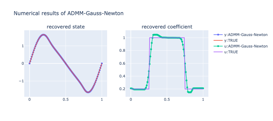
(a) Recovered state and reaction coefficient by the ADMM-Gauss-Newton

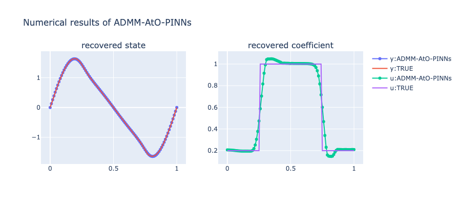
(b) Recovered state and reaction coefficient by Algorithm 4

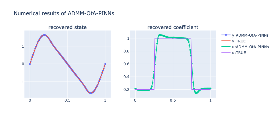
(c) Recovered state and reaction coefficient by Algorithm 5

4. Control constrained optimal control of the Burgers equation

As a simplified model for convection-diffusion phenomena, the Burgers equation plays a crucial role in diverse physical problems such as shock waves, supersonic flow, traffic flows, and acoustic transmission. Its study usually serves as a first approximation to more complex convection diffusion phenomena. Hence, numerical study for the optimal control of the Burgers equation is important for the development of numerical methods for optimal control of more complicated models in fluid dynamics like the Navier–Stokes equations. We refer to e.g., [65, 66] for more discussions.

4.1. Optimal Control Model

Let $\Omega=(0,1)$, we consider the control constrained optimal control of the stationary Burgers equation as that in [18]:

(4.1) $$\left\{\begin{aligned} \min&\frac{1}{2}\|y-y_{d}\|^{2}_{L^{2}(\Omega)}+\frac{\alpha}{2}\|u\|^{2}_{L^{2}(\omega)}+I_{U_{ad}}(u)\\ \text{s.t.}&-\nu y^{\prime\prime}+yy^{\prime}=\chi_{\omega}u\quad\text{in}~{}(0,1),\\ &\qquad y(0)=y(1)=0.\end{aligned}\right.$$

Above, the regularization parameter $\alpha>0$ and the parameter $\nu>0$ denotes the viscosity coefficient of the fluid, which is equal to $\frac{1}{Re}$ with $Re$ the Reynolds number. The target function $y_{d}\in H^{1}(\Omega)$ is given, $\chi_{\omega}$ is the characteristic function of $\omega\subset\Omega$ defined by $\chi_{\omega}(x)=1$ if $x\in\omega$ and $\chi_{\omega}(x)=0$ otherwise, and $I_{U_{ad}}$ is the indicator function of the control set $U_{ad}$ defined by

$$U_{ad}=\{u\in L^{2}(\Omega)|a\leq u(x)\leq b,~{}\text{a.e.~{}in}~{}\omega\},$$

where $a$ and $b$ are given constants. The optimal control of the Burgers equation has been extensively studied in the literature, see e.g., [18, 65, 66] and references therein. In particular, a complete analysis of the optimal control of the Burgers equation was given in [65] and some numerical studies can be referred to [18].

4.2. ADMM-PINNs for (4.1)

Let $y(u)$ be the solution of the state equation (6.2) corresponding to $u$. By introducing $z\in L^{2}(\omega)$ satisfying $u=z$, problem (4.1) can be reformulated as

(4.2) $$\underset{u,z\in L^{2}(\omega)}{\min}{} \frac{1}{2}\|y(u)-y_{d}\|^{2}_{L^{2}(\Omega)}+\frac{\alpha}{2}\|u\|^{2}_{L^{2}(\omega)}+I_{U_{ad}}(z),\quad\text{s.t.}~{} ~{}u=z.$$

The augmented Lagrangian functional associated with (4.2) is defined as

$$L_{\beta}^{BC}(u,z;\lambda)=\frac{1}{2}\|y(u)-y_{d}\|^{2}_{L^{2}(\Omega)}+\frac{\alpha}{2}\|u\|^{2}_{L^{2}(\omega)}+I_{U_{ad}}(z)-(\lambda,u-z)_{L^{2}(\omega)}+\frac{\beta}{2}\|u-z\|_{L^{2}(\omega)}^{2}.$$

Implementing the ADMM to problem (4.2) yields the following iterative scheme:

(4.3a) $$u^{k+1}=\arg\min_{u\in L^{2}(\omega)}L_{\beta}^{BC}(u,z^{k};\lambda^{k}),$$

(4.3b) $$z^{k+1}=\arg\min_{z\in L^{2}(\omega)}L_{\beta}^{BC}(u^{k+1},z;\lambda^{k}),$$

(4.3c) $$\lambda^{k+1}=\lambda^{k}-\beta(u^{k+1}-z^{k+1}).$$

It is easy to show that the $z$-subproblem (4.3b) reads as

$$z^{k+1}=\arg\min_{z\in L^{2}(\omega)}I_{U_{ad}}(z)-(\lambda^{k},u^{k+1}-z)_{L^{2}(\omega)}+\frac{\beta}{2}\|u^{k+1}-z\|_{L^{2}(\omega)}^{2},$$

which has a closed-form solution $z^{k+1}=\mathbb{P}_{U_{ad}}(u^{k+1}-\frac{\lambda^{k}}{\beta}).$ Moreover, the $u$-subproblem (4.3a) can be reformulated as the following unconstrained optimal control problem

$$\min_{y\in L^{2}(\Omega),u\in L^{2}(\omega)}\mathcal{J}^{k}_{BC}(y,u):=\frac{1}{2}\|y-y_{d}\|^{2}_{L^{2}(\Omega)}+\frac{\alpha}{2}\|u\|^{2}_{L^{2}(\omega)}-(\lambda^{k},u-z^{k})_{L^{2}(\omega)}+\frac{\beta}{2}\|u-z^{k}\|_{L^{2}(\omega)}^{2},$$

subject to the Burgers equation in (4.1). Also, if $u$ is a local optimal solution of problem (4.3a), and $y$ and $p$ are the corresponding state and adjoint variables, then they satisfy the following first-order optimality system:

(4.4) $$\left\{\begin{aligned} &p|_{\omega}+(\alpha+\beta)u-\lambda^{k}-\beta z^{k}=0,\\ &-\nu y^{\prime\prime}+yy^{\prime}=\chi_{\omega}u~{}\text{in}~{}(0,1),~{}y(0)=y(1)=0,\\ &-\nu p^{\prime\prime}-yp^{\prime}=y-y_{d}~{}\text{in}~{}(0,1),~{}p(0)=p(1)=0.\end{aligned}\right.$$

Using the relation $u=\frac{1}{\alpha+\beta}(-p|_{\omega}+\lambda^{k}+\beta z^{k})$, we can remove the control $u$ in (4.4) and obtain the following reduced optimality system:

(4.5) $$\left\{\begin{aligned} &-\nu y^{\prime\prime}+yy^{\prime}=\chi_{\omega}(\frac{1}{\alpha+\beta}(-p|_{\omega}+\lambda^{k}+\beta z^{k}))~{}\text{in}~{}(0,1),~{}y(0)=y(1)=0,\\ &-\nu p^{\prime\prime}-yp^{\prime}=y-y_{d}~{}\text{in}~{}(0,1),~{}p(0)=p(1)=0.\end{aligned}\right.$$

As discussed in Section 2.2, the $u$-subproblem (4.3a) can be solved by Algorithm 1 or 2. Accordingly, we obtain two ADMM-PINNs algorithms for solving problem (4.1) and present them in Algorithms 6 and 7, respectively. Note that Algorithm 7 is implemented with the reduced optimality system (4.5), instead of the full optimality system (4.4).

Algorithm 6 ADMM-AtO-PINNs for (4.1)

1:  Input: $\beta>0$, $z^{0},\lambda^{0},\bm{\theta}_{y}^{0},\bm{\theta}_{u}^{0}$, $w_{i}>0$, $w_{b}>0$, $w_{o}>0$ and $w_{e}>0$.

2:  for $k\geq 1$ do

3:     Choose training sets $\mathcal{T}_{i}=\mathcal{T}_{i}^{\omega}\cup\mathcal{T}_{i}^{\Omega/\omega}\subset\Omega$ with $\mathcal{T}_{i}^{\omega}\subset\omega$ and $\mathcal{T}_{i}^{\Omega/\omega}\subset\Omega/\omega$.

4:     Specify a loss function by summing the weighted $L_{2}$ norm of both the equation and boundary condition residuals

$$\mathcal{L}_{PDE}(\bm{\theta}_{y},\bm{\theta}_{u})=\frac{w_{i}}{|\mathcal{T}_{i}|}\sum_{x\in\mathcal{T}_{i}}|-\nu\frac{d^{2}\hat{y}(x;\bm{\theta}_{y})}{dx^{2}}+\hat{y}(x;\bm{\theta}_{y})\frac{d\hat{y}(x;\bm{\theta}_{y})}{dx}-\chi_{\omega}\hat{u}(x;\bm{\theta}_{u})|^{2}+\frac{w_{b}}{2}(|\hat{y}(0;\bm{\theta}_{y})|^{2}+|\hat{y}(1;\bm{\theta}_{y})|^{2}),$$

and a loss function corresponding to the objective functional $\mathcal{J}_{IRC}^{k}$:

$$\mathcal{J}_{BC}^{k}(\bm{\theta}_{y},\bm{\theta}_{u})= \frac{1}{|\mathcal{T}_{i}|}\sum_{x\in\mathcal{T}_{i}}\frac{1}{2}|\hat{y}(x;\bm{\theta}_{y})-y_{d}(x)|^{2}$$

$$+\frac{1}{|\mathcal{T}_{i}^{\omega}|}\sum_{x\in\mathcal{T}_{i}^{\omega}}\left\{\frac{\alpha}{2}|\hat{u}(x;\bm{\theta}_{u})|^{2}-|\lambda(x)(\hat{u}(x;\bm{\theta}_{u})-z^{k}(x))|+\frac{\beta}{2}|\hat{u}(x;\bm{\theta}_{u})-z^{k}(x)|^{2}\right\}.$$

5:     Train the neural networks to update the parameters $\bm{\theta}_{y}^{k+1}$ and $\bm{\theta}_{u}^{k+1}$ by minimizing the following total loss function

$$\mathcal{L}_{total}^{k}(\bm{\theta}_{y},\bm{\theta}_{u})=w_{o}\mathcal{J}_{BC}^{k}(\bm{\theta}_{y},\bm{\theta}_{u})+w_{e}\mathcal{L}_{PDE}(\bm{\theta}_{y},\bm{\theta}_{u}).$$

6:     Update $z^{k+1}$ by $z^{k+1}(x)=\mathbb{P}_{U_{ad}}(\hat{u}(x;\bm{\theta}_{u}^{k+1})-\frac{\lambda^{k}(x)}{\beta})$.

7:     $\lambda^{k+1}(x)=\lambda^{k}-\beta(\hat{u}(x;\bm{\theta}_{u}^{k+1})-z^{k+1}(x))$.

8:  end for

9:  Output: Parameters $(\bm{\theta}_{y}^{*},\bm{\theta}_{u}^{*})$ and hence approximate solutions $\hat{y}(x;\bm{\theta}^{*}_{y})$ and $\hat{u}(x;\bm{\theta}^{*}_{u})$.

Algorithm 7 ADMM-OtA-PINNs for (4.1)

1:  Input: $\beta>0$, $z^{0},\lambda^{0},\bm{\theta}_{y}^{0},\bm{\theta}_{p}^{0}$, $w_{y}>0,w_{p}>0,w_{i}>0$ and $w_{b}>0$.

2:  for $k\geq 1$ do

3:     Choose a training set $\mathcal{T}_{i}\subset\Omega$.

4:     Specify a loss function by summing the weighted $L_{2}$ norm residuals of (4.5):

$$\mathcal{L}_{OS}(\bm{\theta}_{y},\bm{\theta}_{p})=w_{y}\Big{(}\frac{w_{i}}{|\mathcal{T}_{i}|}\sum_{x\in\mathcal{T}_{i}}|-\nu\frac{d^{2}\hat{y}(x;\bm{\theta}_{y})}{dx^{2}}+\hat{y}(x;\bm{\theta}_{y})\frac{d\hat{y}(x;\bm{\theta}_{y})}{dx}$$

$$\qquad\qquad\qquad\qquad-\chi_{\omega}\left(\frac{1}{\alpha+\beta}\left(-\hat{p}(x;\bm{\theta}_{p})|_{\omega}+\lambda^{k}(x)+\beta z^{k}(x)\right)\right)|^{2}+\frac{w_{b}}{2}(|\hat{y}(0;\bm{\theta}_{y})|^{2}+|\hat{y}(1;\bm{\theta}_{y})|^{2})\Big{)}$$

$$+w_{p}\Big{(}\frac{w_{i}}{|\mathcal{T}_{i}|}\sum_{x\in\mathcal{T}_{i}}|-\nu\frac{d^{2}\hat{p}(x;\bm{\theta}_{p})}{dx^{2}}-\hat{y}(x;\bm{\theta}_{y})\frac{d\hat{p}(x;\bm{\theta}_{p})}{dx}-(\hat{y}(x;\bm{\theta}_{y})-y_{d}(x))|^{2}+\frac{w_{b}}{2}(|\hat{p}(0;\bm{\theta}_{p})|^{2}+|\hat{p}(1;\bm{\theta}_{p})|^{2})\Big{)}.$$

5:     Train the neural networks to update the parameters $\bm{\theta}_{y}^{k+1}$ and $\bm{\theta}_{p}^{k+1}$ by minimizing $\mathcal{L}_{OS}(\bm{\theta}_{y},\bm{\theta}_{p})$, and update $u^{k+1}$ by

$$u^{k+1}(x)=\frac{1}{\alpha+\beta}(-\hat{p}(x;\bm{\theta}_{p}^{k+1})|_{\omega}+\lambda^{k}(x)+\beta z^{k}(x))$$

6:     Update $z^{k+1}$ by $z^{k+1}(x)=\mathbb{P}_{U_{ad}}(u^{k+1}(x)-\frac{\lambda^{k}(x)}{\beta})$

7:     $\lambda^{k+1}(x)=\lambda^{k}(x)-\beta(u^{k+1}(x)-z^{k+1}(x))$.

8:  end for

9:  Output: Parameters $(\bm{\theta}_{y}^{*},\bm{\theta}_{p}^{*})$ and solutions $\hat{y}(x;\bm{\theta}^{*}_{y})$ and $\hat{u}(x)=\frac{1}{\alpha+\beta}(-\hat{p}(x;\bm{\theta}_{p}^{*})|_{\omega}+\lambda^{k}(x)+\beta z^{k}(x))$.

4.3. Numerical Results for the Control Constrained Optimal Control of the Burgers Equation (4.1)

In this subsection, we test the control constrained optimal control of the Burgers equation (4.1) and numerically verify the effectiveness of the proposed Algorithms 6 and 7.

Example 2. We consider the example given in [18]. In particular, we set $\Omega=(0,1)$, $\omega=\Omega$, and $\nu=\frac{1}{12},\alpha=0.1,a=-\infty,b=0.3$, and $y_{d}=0.3$ in problem (4.1).

For the implementation of PINNs, we approximate $u$ by a fully-connected feed-forward neural network $\hat{u}(x,\bm{\theta}_{u})$. Moreover, $y$ and $p$ are respectively approximated by $\hat{y}(x;\bm{\theta}_{y})=x(x-1)\mathcal{NN}(x;\bm{\theta}_{y})$ and $\hat{p}(x;\bm{\theta}_{p}=x(x-1)\mathcal{NN}(x;\bm{\theta}_{p})$, with $\mathcal{NN}(x;\bm{\theta}_{y})$ and $\mathcal{NN}(x;\bm{\theta}_{p})$ being fully-connected feed-forward neural networks, so that the boundary conditions $y(0)=y(1)=0$ and $p(0)=p(1)=0$ can be satisfied automatically. Hence, we set $w_{b}=0$. All other weights in the loss function are set to be 1. All the neural networks consist of 4 hidden layers with 50 neurons per hidden layer and hyperbolic tangent activation functions. To evaluate the loss, we take the training sets $\mathcal{T}_{i}\subset\Omega$ as the grid nodes of the lattice generated by uniformly partitioning $\Omega=(0,1)$ with mesh size $h=1/100$. To train the neural networks, we first implement 5000 iterations of the Adam [38] with learning rate $\eta=10^{-3}$ to obtain good guesses of the parameters and then switch to the L-BFGS [49] with a strong Wolfe line search strategy for 1000 iterations to achieve higher accuracy. The neural network parameters are initialized using the default initializer of Pytorch. In the implementation of Algorithms 6 and 7, we execute 20 outer ADMM iterations with $\beta=1e-1,z^{0}=0$, and $\lambda^{0}=0$.

Moreover, to validate the effectiveness of the Algorithms 6 and 7, we compare our results with the reference ones obtained by high-fidelity traditional numerical methods based on FEM. To be concrete, problem (4.1) is first discretized by FEM and then is solved by the SSN method [18]. A FEM-SSN method is thus specified for solving (4.1). To implement the FEM, the domain $\Omega=(0,1)$ is uniformly partitioned with mesh size $h=1/100$.

Figure 2 shows the computed optimal controls and states by different algorithms. We observe that the states obtained by all the algorithms are almost the same. The control constraint $u(x)\leq 0.3$ a.e. in $\Omega$ is satisfied in all cases. Furthermore, the control computed by Algorithm 7 is so close to the one by the FEM-SSN and they cannot be visually distinguished. However, we note that the control computed by Algorithm 6 is different. A possible reason is that problem (4.1) has a non-unique solution due to its nonconvexity, and Algorithm 6 finds a different control that solves the problem. All these results validate the effectiveness of our proposed ADMM-PINNs algorithms.

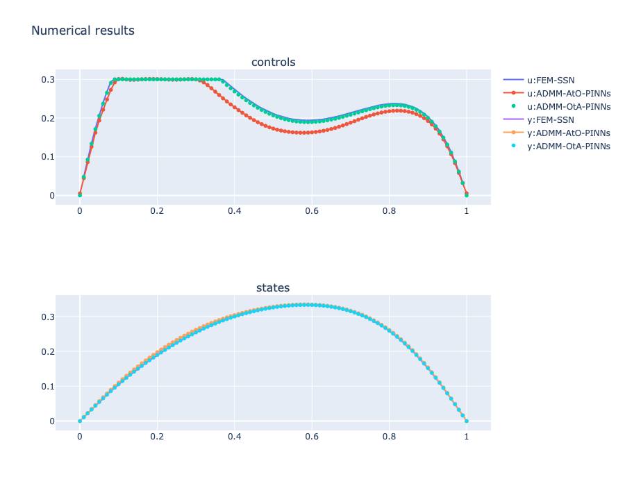
Figure 2. Numerical results for Example 2: control constrained optimal control of the Burgers equation

5. Discontinuous Source Identification for Elliptic PDEs

5.1. Problem Statement

In this section, we discuss the implementation of Algorithm 3 to discontinuous source identification for elliptic PDEs. In particular, we study the problem of identifying a discontinuous source in a prototypical elliptic PDE from Dirichlet boundary observation data:

(5.1) $$\min_{u,y} ~{}\Big{\{}\frac{1}{2}\int_{\partial\Omega}|y-y^{\delta}|^{2}dx+\gamma\int_{\omega}|\nabla u|dx\Big{\}},$$

s.t. $$-\Delta y+cy=u~{}\text{in}~{}\Omega,~{}\frac{\partial y}{\partial n}=0~{}\text{on}~{}\partial\Omega,$$

$$~{}u=0~{}\text{in}~{}\Omega/\omega$$

where $\Omega$ is a bounded domain in $\mathbb{R}^{d}$ ($d\geq 1$) with a piecewise smooth boundary $\partial\Omega$, $\omega\subset\Omega$ is an open set. The constant coefficient $c>0$ is given, $u$ is the unknown source, and $n$ denotes the outwards pointing unit normal vector of the boundary $\partial\Omega$. Here, we consider the case that some observation data, denoted by $y^{\delta}\in L^{2}(\Omega)$, of the solution $y$ on the boundary $\partial\Omega$ is available subject to some noise with the noisy level $\delta>0$. In other words, we attempt to use the Dirichlet boundary observation data $\ y^{\delta}$ to identify the unknown source $u$ by solving (5.1). Moreover, $\frac{1}{2}\int_{\partial\Omega}|y-y^{\delta}|^{2}\mathrm{d}x$ is a data-fidelity term, $\int_{\omega}|\nabla u|dx$ is the TV-regularization defined by (2.12), and $\gamma>0$ is a regularization parameter. Problem (5.1) and its variants have found various applications in crack determination [1], electroencephalography [2] and inverse electrocardiography [69].

5.2. ADMM-PINNs for (5.1)

For any given $u\in L^{2}(\Omega)$, let $y(u)$ be the solution of the equation

$$-\Delta y+cy=u~{}\text{in}~{}\Omega,~{}\frac{\partial y}{\partial n}=0~{}\text{on}~{}\partial\Omega.$$

By introducing an auxiliary variable $z$ such that $u=z$, we can reformulate problem (5.1) as

(5.2) $$\min_{u,z}~{}\frac{1}{2}\int_{\partial\Omega}|y(u)-y^{\delta}|^{2}\mathrm{d}x+\gamma\int_{\omega}|\nabla z|dx,\quad\text{s.t.}~{}u=z~{}\text{in}~{}\Omega,~{}z=0~{}\text{in}~{}\Omega/\omega$$

The augmented Lagrangian functional associated with (5.2) is defined

$$L_{\beta}^{SI}(u,z;\lambda)=\frac{1}{2}\int_{\partial\Omega}|y(u)-y^{\delta}|^{2}\mathrm{d}x+\gamma\int_{\omega}|\nabla z|dx-(\lambda,u-z)_{L^{2}(\Omega)}+\frac{\beta}{2}\|u-z\|_{L^{2}(\Omega)}^{2},$$

where $\beta>0$ is a penalty parameter. Then the ADMM iterative scheme for solving (5.1) reads as

(5.3a) $$u^{k+1}=\arg\min_{u}L_{\beta}^{SI}(u,z^{k};\lambda^{k}),$$

(5.3b) $$z^{k+1}=\arg\min_{z=0~{}\text{in}~{}\Omega/\omega}L_{\beta}^{SI}(u^{k+1},z;\lambda^{k}),$$

(5.3c) $$\lambda^{k+1}=\lambda^{k}-\beta(u^{k+1}-z^{k+1}).$$

We first note that the $z$-subproblem (5.3b) is a TV-regularized optimization problem

(5.4) $$z^{k+1}=\arg\min_{z\in L^{2}(\omega)}\gamma\int_{\omega}|\nabla z|dx+\frac{\beta}{2}\|z-(u^{k+1}-\frac{\lambda^{k}}{\beta})\|^{2},\quad\text{in}~{}\omega,\\$$

and $z^{k+1}=0$ in ${\Omega/\omega}$. We further assume that $\omega\subset\mathbb{R}^{2}$ is a rectangular domain. Then, inspired by [63], problem (5.4) after some proper discretization can be solved by a pre-trained deep CNN. To elaborate, let $R(z):=\int_{\omega}|\nabla z|dx$, then the proximal operator of $\gamma R(z)$ is given by

$$\text{Prox}_{\gamma R(z)}(v)=\arg\min_{z\in L^{2}(\omega)}\Big{\{}\gamma R(z)+\frac{1}{2}\|z-v\|_{L^{2}(\omega)}^{2}\Big{\}},~{}\forall v\in L^{2}(\omega).$$

Then, the solution of (5.4) can be expressed as

$$z^{k+1}=\text{Prox}_{\frac{\gamma}{\beta}R(z)}(u^{k+1}-\frac{\lambda^{k}}{\beta})\quad\text{in}~{}\omega.$$

Following [55], $\text{Prox}_{\frac{\gamma}{\beta}R(z)}$ can be interpreted as an image denoising operator.

Suppose that the domain $\omega$ is uniformly partitioned with mesh size $h$, and $\bm{x}=\{x_{i}\}_{i=1}^{N}$ are the grid nodes of the resulting lattice. For any function $q:\omega\subset\mathbb{R}^{2}\rightarrow\mathbb{R}$, we let $q_{h}:\mathbb{R}^{2}\rightarrow\mathbb{R}$ defined on the lattice be a finite approximation of $q$. Then, there exists a one-to-one mapping between $q_{h}$ and an $m\times n$ raster image $\mathcal{I}$ ($m\times n=N$), where the gray value at pixel $x_{i}$ of the image $\mathcal{I}$ corresponds to the value of the function $q_{h}$ at node $x_{i}$. Then, pre-trained deep CNNs, which have been widely used for various image denoising problems, can be applied. For this purpose, let $\mathcal{M}$ denote the mapping from $q_{h}$ to the raster image $\mathcal{I}$, and $\mathcal{C}_{\sigma}$ represents a pre-trained deep CNN with $\sigma$ the variance of the noise used for training the CNN. Solving problem (5.4) by a pre-trained deep CNN is summarized in Algorithm 8. Note that once a pre-trained deep CNN is applied, the parameter $\gamma$ is not needed any more and its role will be replaced by the denoising parameter $\sigma$.

Algorithm 8 A deep CNN-based method for (5.4).

1:  $\mathcal{I}^{k+1}_{input}:=\mathcal{M}(u_{h}^{k+1}(\bm{x})-\frac{\lambda_{h}^{k}(\bm{x})}{\beta})$.

2:  $\mathcal{I}^{k+1}_{output}:=\mathcal{C}_{\sigma}(\mathcal{I}_{input}^{k+1})$.

3:  $z_{h}^{k+1}(\bm{x})=\mathcal{M}^{-1}(\mathcal{I}^{k+1}_{output})$.

The $u$-subproblem (5.3a) can be reformulated as the following PDE-constrained optimization problem:

$$\min\mathcal{J}^{k}_{SI}(y,u):=\frac{1}{2}\int_{\partial\Omega}|y-y^{\delta}|^{2}\mathrm{d}x-(\lambda^{k},u-z^{k})+\frac{\beta}{2}\|u-z^{k}\|^{2},$$

subject to the equation in (5.1). Its first-order optimality system reads as:

(5.5) $$\left\{\begin{aligned} &p+\beta u-\lambda^{k}-\beta z^{k}=0,\\ &-\Delta y+cy=u\text{~{}in~{}}\Omega,~{}\frac{\partial y}{\partial n}=0\text{~{}on~{}}\partial\Omega,\\ &-\Delta p+cp=0\text{~{}in~{}}\Omega,~{}\frac{\partial p}{\partial n}=y-y^{\delta}\text{~{}on~{}}\partial\Omega,\end{aligned}\right.$$

where $u$ is the solution to the $u$-subproblem (5.3a), $y$ is the corresponding solution of the equation in (5.1), and $p$ is the adjoint variable. Furthermore, using the relation $u=\frac{-p+\lambda^{k}+\beta z^{k}}{\beta}$, we can rewrite (5.5) as

(5.6) $$\left\{\begin{aligned} &-\Delta y+cy=\frac{-p+\lambda^{k}+\beta z^{k}}{\beta}\text{~{}in~{}}\Omega,~{}\frac{\partial y}{\partial n}=0\text{~{}on~{}}\partial\Omega,\\ &-\Delta p+cp=0\text{~{}in~{}}\Omega,~{}\frac{\partial p}{\partial n}=y-y^{\delta}\text{~{}on~{}}\partial\Omega.\end{aligned}\right.$$

As discussed in Section 2.2, the $u$-subproblem (5.3a) can be solved by applying Algorithm 1 or Algorithm 2. Accordingly, we can obtain two ADMM-PINNs algorithms for solving problem (5.1). However, it was empirically observed that, when the ADMM-AtO-PINNs is applied, the corresponding neural networks are hard to train and the numerical results are not satisfactory. A main reason is that the balance between the objective function and the PDE losses is sensitive and unstable for this case. To address this issue, much more effort is needed to find suitable loss weights, which is beyond the scope of the paper. Hence, we only focus on the application of the ADMM-OtA-PINNs to problem (5.1) and the resulting algorithm is presented in Algorithm 9.

Algorithm 9 ADMM-OtA-PINNs for (5.1)

1:  Input: $\beta>0$, $z^{0},\lambda^{0},\bm{\theta}_{y}^{0},\bm{\theta}_{p}^{0}$, $w_{u}>0,w_{y}>0,w_{p}>0,w_{i}>0$ and $w_{b}>0$.

2:  for $k\geq 1$ do

3:     Choose training sets $\mathcal{T}_{i}\subset\Omega$ and $\mathcal{T}_{b}\subset\partial\Omega$.

4:     Specify a loss function by summing the weighted $L_{2}$ norm of (5.6):

$$\mathcal{L}_{OS}(\bm{\theta}_{y},\bm{\theta}_{p})= w_{y}\left(\frac{w_{i}}{|\mathcal{T}_{i}|}\sum_{x\in\mathcal{T}_{i}}|-\Delta\hat{y}(x;\bm{\theta}_{y})+c\hat{y}(x;\bm{\theta}_{y})-\frac{-\hat{p}(x;\bm{\theta}_{p})+\lambda^{k}(x)+\beta z^{k}(x)}{\beta}|^{2}+\frac{w_{b}}{|\mathcal{T}_{b}|}\sum_{x\in\mathcal{T}_{b}}|\frac{\partial\hat{y}(x;\bm{\theta}_{y})}{\partial n}|^{2}\right)$$

$$+w_{p}\left(\frac{w_{i}}{|\mathcal{T}_{i}|}\sum_{x\in\mathcal{T}_{i}}|-\Delta\hat{p}(x;\bm{\theta}_{p})+c\hat{p}(x;\bm{\theta}_{p})|^{2}+\frac{w_{b}}{|\mathcal{T}_{b}|}\sum_{x\in\mathcal{T}_{b}}|\frac{\partial\hat{p}(x;\bm{\theta}_{p})}{\partial n}-(\hat{y}(x;\bm{\theta}_{y})-y^{\delta}(x))|^{2}\right).$$

5:     Train the neural networks to update the parameters $\bm{\theta}_{y}^{k+1}$, and $\bm{\theta}_{p}^{k+1}$ by minimizing the loss function $\mathcal{L}_{OS}(\bm{\theta}_{y},\bm{\theta}_{p})$.

6:     Update $u^{k+1}$ by $u^{k+1}(x)=\frac{-\hat{p}(x;\bm{\theta}_{p}^{k+1})+\lambda^{k}(x)+\beta z^{k}(x)}{\beta}$.

7:     Update $z^{k+1}$ by (2.14a)-(2.14c) with $z_{0}=z^{k},\mu_{0}=0$.

8:     $\lambda^{k+1}(x)=\lambda^{k}(x)-\beta(\hat{u}(x;\bm{\theta}_{u}^{k+1})-z^{k+1}(x))$.

9:  end for

10:  Output: Parameters $(\bm{\theta}_{y}^{*},\bm{\theta}_{p}^{*})$ and approximate solutions $\hat{y}(x;\bm{\theta}^{*}_{y})$ and $\hat{u}(x)=\frac{-\hat{p}(x;\bm{\theta}_{p}^{*})+\lambda^{k}(x)+\beta z^{k}(x)}{\beta}$.

5.3. Numerical Results for the Source Identification Problem (5.1)

In this section, we devote ourselves to showing the numerical results of Algorithm 9 for solving a source identification problem.

Example 3. We set $\Omega=(0,1)\times(0,1)$, $\omega=\omega_{1}\cup\omega_{2}$ with $\omega_{1}=(0.25,0.5)\times(0.25,0.75),\omega_{2}=(0.5,0.75)\times(0.25,0.75)$ and $c=1$. We take the true source term $u$ as

$$u_{true}(x)=3\chi_{w_{1}}(x)-9\chi_{\omega_{2}}(x),$$

where $\chi_{w_{1}}$ and $\chi_{w_{2}}$ are the characteristic functions of $\omega_{1}$ and $\omega_{2}$, respectively. The observed data $y^{\delta}=y_{true}+\delta\|y_{true}\|\text{rand}(x)$, where $\delta=0.1$, $y_{true}$ is the solution of equation (5.1) corresponding to $u_{true}$, and $\text{rand}(x)$ is a standard normal distributed random function. In our numerical experiments, $y_{true}$ is the solution of (3.1) obtained from $u_{true}$ by FEM. To implement the FEM used for this example, the domain $\Omega$ is uniformly triangulated with mesh size $h=1/64$.

For the implementation of PINNs, we approximate $y$ and $p$ by $\hat{y}(x;\bm{\theta}_{y})=\mathcal{NN}(x;\bm{\theta}_{y})$ and $\hat{p}(x;\bm{\theta}_{p})=\beta\mathcal{NN}(x;\bm{\theta}_{p})$, with $\mathcal{NN}(x;\bm{\theta}_{y})$ and $\mathcal{NN}(x;\bm{\theta}_{p})$ being fully-connected feed-forward neural networks. All the neural networks consist of 3 hidden layers with 32 neurons per hidden layer and hyperbolic tangent activation functions. To evaluate the loss, we take the training sets $\mathcal{T}_{i}\subset\Omega$ as $31\times 31$ uniformly sampled points and $\mathcal{T}_{b}\subset\partial\Omega$ as $4\times 128$ uniformly sampled points. The weights $\frac{w_{i}}{|\mathcal{T}_{i}|}$, $\frac{w_{b}}{|\mathcal{T}_{b}|}$,$w_{o}$, $w_{e}$, $w_{y}$, and $w_{p}$ are set to be 1. To train the neural networks, we first execute the Adam [38] with learning rate $\eta=10^{-4}$ for 20000 iterations to obtain good guesses of the neural network parameters and then switch to the L-BFGS [49] with a strong Wolfe line search strategy for 1000 iterations to achieve higher accuracy. The neural network parameters are initialized using the default initializer of Pytorch.

For the CNN used in this example, we use the same network architecture, the same training dataset, and the PyTorch version of the original code as [74] (see https://github.com/cszn/DnCNN for the original code and https://github.com/cszn/KAIR for the PyTorch version) to train 30 CNNs for the cases where $\sigma=1,2,\cdots,30$. Hence, $C_{\sigma}$ in Algorithm 8 is chosen as one of these pre-trained 30 CNNs with a specified value of $\sigma$. According to our tests, $\sigma=24$ is the best choice. The mapping $\mathcal{M}$ in Algorithm 8 is specified as $\mathcal{M}(z_{h})=(\bm{z}+10)/20\times 256$, where $\bm{z}=z_{h}(\bm{x})$ and $\mathcal{I}$ is a raster image. To avoid the gray values of the raster image exceeding the range, we added a projection to ensure the gray values of $\mathcal{I}$ strictly fall in $(0,255)$.

Moreover, to validate the effectiveness of Algorithm 9, we compare our results with the reference ones obtained by a high-fidelity FEM-based numerical method. To be concrete, the subproblem (5.3a) is first discretized by FEM and then is solved by a conjugate gradient (CG) method. An ADMM-CG algorithm is thus specified for solving (5.1). Similar methods can be found in [25, 26]. For implementing both Algorithms 9 and the ADMM-CG, we execute 350 ADMM iterations with $\beta=5e-2,z^{0}=0,\lambda^{0}=0$.

We observe from the results that Algorithm 9 is robust to the noise level $\delta$. We report the recovered sources and states by different algorithms with $\delta=10\%$ in Figure 3. We can see that even if the noise increases to $10\%$, the identified solutions are still very satisfactory. In particular, the computed states by Algorithm 9 achieve good agreements with the reference one and they cannot be visually distinguished. Moreover, we do not see much difference between the identified source by Algorithm 9 and the one by the ADMM-CG algorithm, which indicates that Algorithm 9 is comparable to traditional FEM-based numerical methods.

Figure 3. Numerical results for Example 3: discontinuous source identification for an elliptic equation. Noise level $\delta=10\%.$ Relative error of $u$: 0.174639 (ADMM-CG), 0.171283 (Algorithm 9)

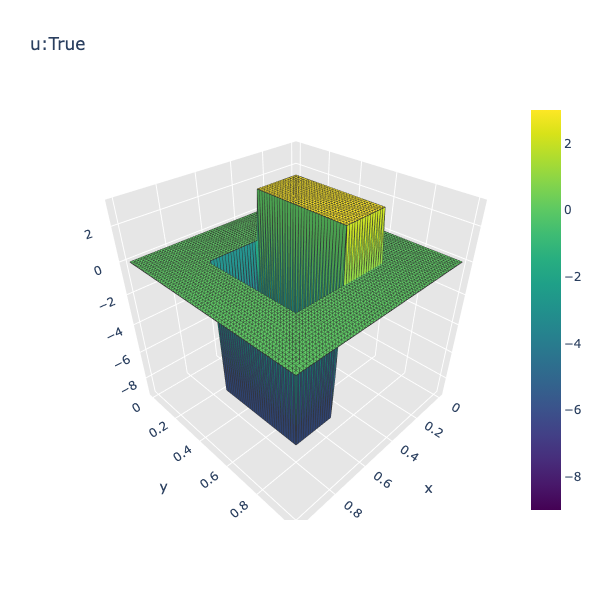
(a) True source

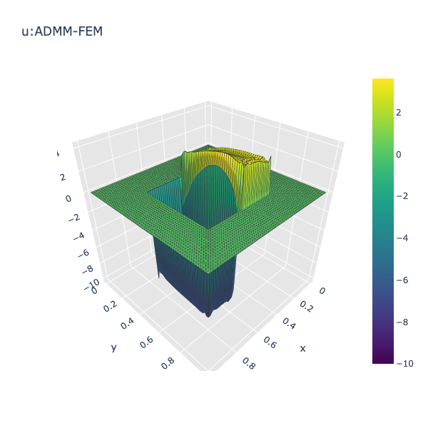
(b) Recovered source by ADMM-CG

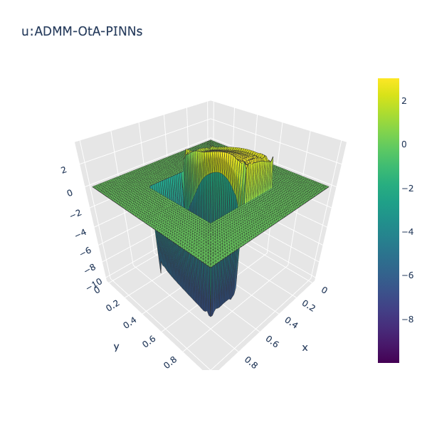
(c) Recovered source by Algorithm 9

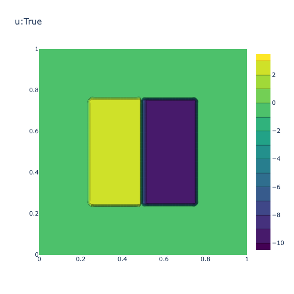
(d) True source

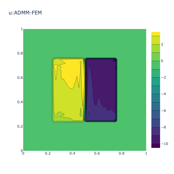
(e) Recovered source by ADMM-CG

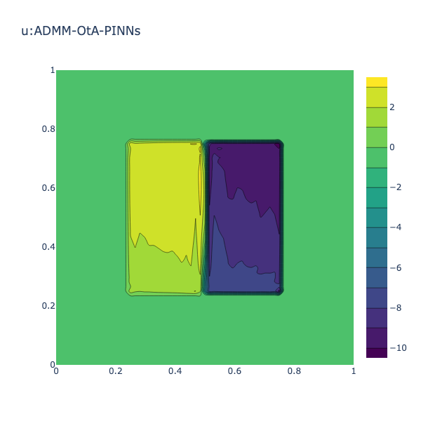
(f) Recovered source by Algorithm 9

(g) True state

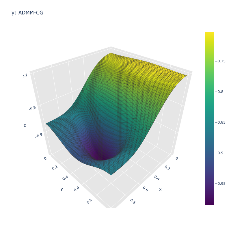
(h) Recovered state by ADMM-CG

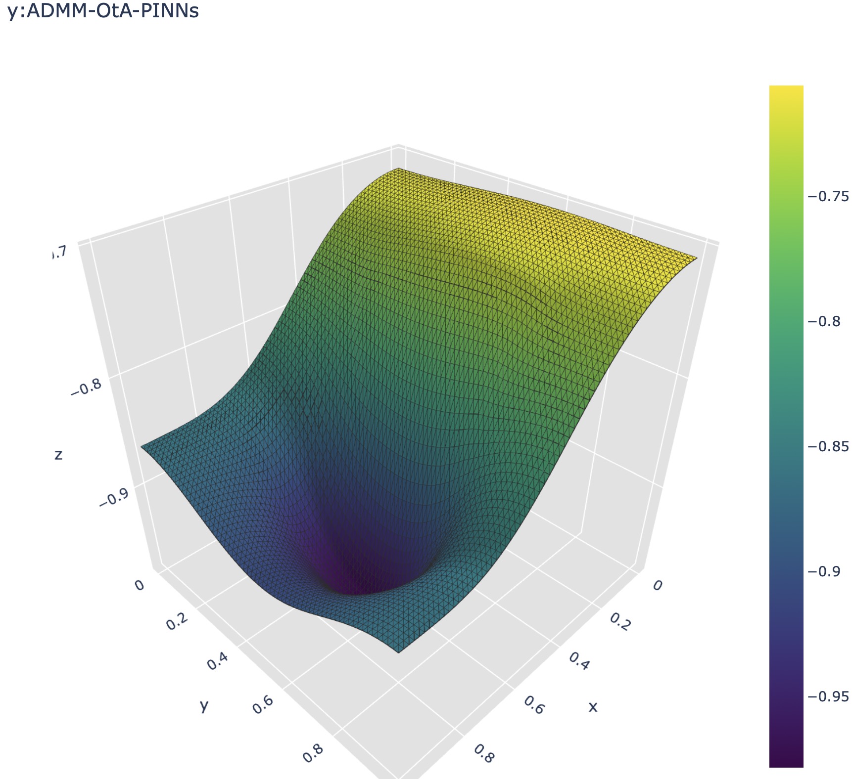
(i) Recovered state by Algorithm 9

6. Sparse optimal control of parabolic equations

In PDE-constrained optimal control problems, we usually can only put the controllers in some small regions instead of the whole domain under investigation. As a consequence, a natural question arises: how to determine the optimal locations and the intensities of the controllers? This concern inspires a class of optimal control problems where the controls are sparse (i.e., they are only non-zero in a small region of the domain); and the so-called sparse optimal control problems are obtained, see [57]. In this section, we consider a parabolic sparse optimal control problem to validate the effectiveness and efficiency of the ADMM-PINNs algorithmic framework.

6.1. Sparse Optimal Control Model

A representative formulation of parabolic sparse optimal control problems can be formulated as:

(6.1) $$\underset{y,u\in L^{2}(Q)}{\min}~{}\frac{1}{2}\|y-y_{d}\|^{2}_{L^{2}(Q)}+\frac{\alpha}{2}\|u\|^{2}_{L^{2}(Q)}+{\rho}\|u\|_{L^{1}(Q)}+I_{U_{ad}}(u),$$

where $y$ and $u$ satisfy the parabolic state equation:

(6.2) $$\left\{\begin{aligned} \frac{\partial y}{\partial t}-\nu\Delta y+c_{0}y=&u+f\quad\text{in}\quad\Omega\times(0,T),\\ y=&0\quad\text{on}\quad\partial\Omega\times(0,T),\\ y(0)=&\varphi.\end{aligned}\right.$$

In (6.1)-(6.2), $\Omega$ is a bounded domain in $\mathbb{R}^{d}$ with $d\geq 1$ and $\partial\Omega$ is its boundary; $Q=\Omega\times(0,T)$ with $0<T<+\infty$; the desired state $y_{d}\in L^{2}(Q)$ and the functions $\phi\in L^{2}(\Omega),f\in L^{2}(Q)$ are given. The constants $\alpha>0$ and $\rho>0$ are regularization parameters. The coefficients $\nu>0$ and $c_{0}\leq 0$ are assumed to be constant. We denote by $I_{U_{ad}}(\cdot)$ the indicator function of the admissible set $U_{ad}$ defined by

$$U_{ad}=\{u\in L^{\infty}(\Omega)|a\leq u(x,t)\leq b,~{}\text{a.e.~{}in}~{}Q\}\subset L^{2}(Q),$$

where $a,b\in L^{2}(\Omega)$ with $a<0<b$ almost everywhere.

Due to the presence of the nonsmooth $L^{1}$-regularization term, the structure of the optimal control of (6.1) differs significantly from what one obtains for the usual smooth $L^{2}$-regularization. Particularly, the optimal control has small support as discussed in [57, 67]. Because of this special structural property, optimal control problems with $L^{1}$-regularization capture important applications in various fields such as optimal actuator placement [57] and impulse control [15]. For example, as studied in [57], if one cannot or does not want to distribute control devices all over the control domain, but wants to place available devices in an optimal way, the solution of the problem (6.1) can give some information about the optimal location of control devices.

6.2. ADMM-PINNs for (6.1)

Let $y(u)$ be the solution of the state equation (6.2) corresponding to $u$. By introducing $z\in L^{2}(Q)$ satisfying $u=z$, problem (6.1) can be reformulated as

(6.3) $$\underset{u,z\in L^{2}(Q)}{\min}{} \frac{1}{2}\|y(u)-y_{d}\|^{2}_{L^{2}(Q)}+\frac{\alpha}{2}\|u\|^{2}_{L^{2}(Q)}+{\rho}\|z\|_{L^{1}(Q)}+I_{U_{ad}}(z),\quad\text{s.t.}~{} ~{}u=z.$$

The augmented Lagrangian functional associated with (6.3) is defined as

$$L_{\beta}^{SC}(u,z;\lambda)=\frac{1}{2}\|y(u)-y_{d}\|^{2}_{L^{2}(Q)}+\frac{\alpha}{2}\|u\|^{2}_{L^{2}(Q)}-(\lambda,u-z)_{L^{2}(Q)}+\frac{\beta}{2}\|u-z\|_{L^{2}(Q)}^{2}.$$

Implementing the ADMM to problem (6.3) yields the following iterative scheme:

(6.4a) $$u^{k+1}=\arg\min_{u\in L^{2}(Q)}L_{\beta}^{SC}(u,z^{k};\lambda^{k}),$$

(6.4b) $$z^{k+1}=\arg\min_{z\in L^{2}(Q)}L_{\beta}^{SC}(u^{k+1},z;\lambda^{k}),$$

(6.4c) $$\lambda^{k+1}=\lambda^{k}-\beta(u^{k+1}-z^{k+1}).$$

First, it is easy to show that the $z$-subproblem (6.4b) reads as

$$z^{k+1}=\arg\min_{z\in L^{2}(Q)}I_{U_{ad}}(z)+\rho\|z\|_{L^{1}(Q)}-(\lambda^{k},u^{k+1}-z)_{L^{2}(Q)}+\frac{\beta}{2}\|u^{k+1}-z\|_{L^{2}(Q)}^{2},$$

which has a closed-form solution $z^{k+1}=\mathbb{P}_{U_{ad}}\left(\mathbb{S}_{\frac{\rho}{\beta}}\left(u^{k+1}-\frac{\lambda^{k}}{\beta}\right)\right).$ Moreover, the $u$-subproblem (6.4a) can be reformulated as

(6.5) $$\min_{y,u}\mathcal{J}_{SC}^{k}(y,u):=\frac{1}{2}\|y-y_{d}\|^{2}_{L^{2}(Q)}+\frac{\alpha}{2}\|u\|^{2}_{L^{2}(Q)}-(\lambda^{k},u-z^{k})_{L^{2}(Q)}+\frac{\beta}{2}\|u-z^{k}\|_{L^{2}(Q)}^{2}$$

subject to the state equation (6.2). The first-order optimality system of (6.5) reads as

(6.6) $$\left\{\begin{aligned} &p+(\alpha+\beta)u-\lambda^{k}-\beta z^{k}=0,\\ &\frac{\partial y}{\partial t}-\nu\Delta y+c_{0}y=u+f~{}\text{in}~{}\Omega\times(0,T),\quad y=0~{}\text{on}~{}\partial\Omega\times(0,T),\quad y(0)=\varphi,\\ &-\frac{\partial p}{\partial t}-\nu\Delta p+c_{0}p=y-y_{d}~{}\text{in}~{}\Omega\times(0,T),\quad p=0~{}\text{on}~{}\partial\Omega\times(0,T),\quad p(T)=0,\end{aligned}\right.$$

where $u$ is the optimal solution of problem (6.5), $y$ and $p$ are the corresponding state and adjoint variable, respectively.

As discussed in Section 2.2, the $u$-subproblem (6.4a) can be solved by applying Algorithm 1 or 2. Accordingly, two ADMM-PINNs algorithms can be obtained for solving problem (6.1). However, as mentioned in Section 5, it was empirically observed that, when the ADMM-AtO-PINNs is applied, the corresponding neural networks are hard to train and the numerical results are not satisfactory. This is mainly because that the balance between the objective function and the PDE losses is sensitive and unstable for this case. To address this issue, much more effort is needed to find suitable loss weights, which is beyond the scope of the paper. Hence, we only focus on the application of the ADMM-OtA-PINNs to problem (6.1) and the resulting algorithm is presented in Algorithm 10.

Algorithm 10 ADMM-OtA-PINNs for (6.1)

1:  Input: $\beta>0$, $z^{0},\lambda^{0},\bm{\theta}_{y}^{0},\bm{\theta}_{p}^{0}$.

2:  for $k\geq 1$ do

3:     Choose training sets $\mathcal{T}_{i}\subset\Omega\times(0,T)$, $\mathcal{T}_{b_{1}}\subset\partial\Omega\times(0,T)$, and $\mathcal{T}_{b_{2}}\subset\Omega$.

4:     Specify a loss function by summing the weighted $L_{2}$ norm of the optimality condition (6.6)

(6.7) $$\mathcal{L}_{OS}(\bm{\theta}_{y},\bm{\theta}_{p})=w_{y}\Big{(}\frac{w_{i}}{|\mathcal{T}_{i}|}\sum_{\{x,t\}\in\mathcal{T}_{i}}|\frac{\partial\hat{y}(x,t;\bm{\theta}_{y})}{\partial t}-\nu\frac{\partial^{2}\hat{y}(x,t;\bm{\theta}_{y})}{\partial x^{2}}+c_{0}\hat{y}(x,t;\bm{\theta}_{y})$$

$$\qquad\qquad\qquad\qquad-\frac{1}{\alpha+\beta}\big{(}-\hat{p}(x,t;\bm{\theta}_{p})+\lambda^{k}(x,t)+\beta z^{k}(x,t)\big{)}-f(x,t)|^{2}$$

$$\qquad\qquad\qquad\qquad+\frac{w_{b_{1}}}{|\mathcal{T}_{b_{1}}|}\sum_{\{x,t\}\in\mathcal{T}_{b_{1}}}|\hat{y}(x,t;\bm{\theta}_{y})|^{2}+\frac{w_{b_{2}}}{|\mathcal{T}_{b_{2}}|}\sum_{x\in\mathcal{T}_{b_{2}}}|\hat{y}(x,0;\bm{\theta}_{y})-\varphi(x)|^{2}\Big{)}$$

$$+w_{p}\Big{(}\frac{w_{i}}{|\mathcal{T}_{i}|}\sum_{\{x,t\}\in\mathcal{T}_{i}}|-\frac{\partial\hat{p}(x,t;\bm{\theta}_{p})}{\partial t}-\nu{\Delta\hat{p}(x,t;\bm{\theta}_{p})}+c_{0}\hat{p}(x,t;\bm{\theta}_{p})-\hat{y}(x,t;\bm{\theta}_{y})+y_{d}(x,t)|^{2}$$

$$\qquad\qquad\qquad\qquad+\frac{w_{b_{1}}}{|\mathcal{T}_{b_{1}}|}\sum_{\{x,t\}\in\mathcal{T}_{b_{1}}}|\hat{p}(x,t;\bm{\theta}_{p})|^{2}+\frac{w_{b_{2}}}{|\mathcal{T}_{b_{2}}|}\sum_{x\in\mathcal{T}_{b_{2}}}|\hat{p}(x,0;\bm{\theta}_{p})|^{2}\Big{)}$$

5:     Train the neural networks to update the parameters $\bm{\theta}_{y}^{k+1}$ and $\bm{\theta}_{p}^{k+1}$ by minimizing (6.7), and update $u^{k+1}$ by

$$u^{k+1}(x,t)=\frac{1}{\alpha+\beta}(-\hat{p}(x,t;\bm{\theta}_{p}^{k+1})+\lambda^{k}(x,t)+\beta z^{k}(x,t)).$$

6:     Update $z^{k+1}$ by $z^{k+1}(x,t)=\mathbb{P}_{U_{ad}}\left(\mathbb{S}_{\frac{\rho}{\beta}}\left(u^{k+1}(x,t)-\frac{\lambda^{k}(x,t)}{\beta}\right)\right)$.

7:     Update $\lambda^{k+1}(x,t)=\lambda^{k}(x,t)-\beta(u^{k+1}(x,t)-z^{k+1}(x,t))$.

8:  end for

9:  Output: Parameters $(\bm{\theta}_{y}^{*},\bm{\theta}_{p}^{*})$ and hence approximate solutions $\hat{y}(x,t;\bm{\theta}^{*}_{y})$ and $\hat{u}(x,t)=\frac{1}{\alpha+\beta}(-\hat{p}(x,t;\bm{\theta}_{p}^{*})+\lambda^{k}(x,t)+\beta z^{k}(x,t))$.

6.3. Numerical Results for the Sparse Optimal Control Problem (6.1)

In this subsection, we report some numerical results to validate the effectiveness and efficiency of Algorithm 10 for solving the sparse optimal control problem (6.1).

Example 4. We consider an example of problem (6.1) with a known exact solution. In particular, we set $\Omega=(0,1)^{2},T=1,\nu=1,c_{0}=0,a=-1,b=2,\bar{y}=5\sqrt{\rho}t\sin(3\pi x_{1})\sin(\pi x_{2}),\bar{p}=5\sqrt{\rho}(t-1)\sin(\pi x_{1})\sin(\pi x_{2})$, and

$$\bar{u}=\left\{\begin{aligned} &\max\{\frac{-\bar{p}+\rho}{\alpha},a\}~{}&&\text{in}~{}\{(x,t)\in\Omega\times(0,T):\bar{p}(x,t)>\rho\},\\ &\min\{\frac{-\bar{p}-\rho}{\alpha},b\}~{}&&\text{in}~{}\{(x,t)\in\Omega\times(0,T):\bar{p}(x,t)<-\rho\},\\ &0&&\text{otherwise}.\end{aligned}\right.$$

We further set $f=\frac{\partial\bar{y}}{\partial t}-\Delta\bar{y}-u$ and $y_{d}=\bar{y}-(-\frac{\partial\bar{p}}{\partial t}-\Delta\bar{p}).$ Then it can be shown that $\bar{u}$ is the optimal control of problem (6.1) and $\bar{y}$ is the corresponding optimal state, the details can be referred to [56]

To solve the $u$-subproblem (4.3a) in the PINNs framework, we approximate $y$ and $p$ with fully-connected feed-forward neural networks containing 3 hidden layers of 32 neurons each. The hyperbolic tangent activation function is used in all the neural networks. To evaluate the loss, we uniformly sample $|\mathcal{T}_{i}|=4096$ residual points in the spatial-temporal domain $\Omega\times(0,T)$, and $|\mathcal{T}_{b_{1}}|=1024$ points in $\partial\Omega\times(0,T)$ and $|\mathcal{T}_{b_{2}}|=256$ points in $\Omega$ for the boundary and initial conditions. Note that we reselect the residual points randomly at each ADMM iteration and they can be different from those in previous iterations. The weights are set as $w_{y}=w_{p}=1$, $w_{i}=1$ and $w_{b1}=w_{b2}=5$.

To train the neural networks, we first use the Adam optimizer [38] with learning rate $\eta=10^{-3}$ for 10000 iterations, and then switch to the L-BFGS [49] for 10 iterations. In the implementation of Algorithm 10, we execute 10 ADMM iterations with $\alpha=0.1,\rho=0.8,\beta=0.1$, $z^{0}=0$ and $\lambda^{0}=0$. The computed results are shown in Figures 4 and 5.

A comparison of the computed and exact controls at three different temporal snapshots ($t=0.25,0.5$ and $0.75$) is shown in Figure 5. First, the sparsity of the control can be observed. Moreover, the computed control is very close to the exact one, and they even cannot be visually distinguished in Figure 5. Indeed, we have that the relative error

$$\frac{\|u^{k}(x,t)-\bar{u}(x,t)\|_{L^{2}(Q)}}{\|\bar{u}(x,t)\|_{L^{2}(Q)}}=1.45\%.$$

Furthermore, in our settings, it is easy to see $\bar{u}=0$ in $\{(x,t)\in\Omega\times(0,T):\bar{p}(x,t)|<\rho\}$ and we can show that when $t>t^{*}=0.8211$, $u(x,t)=0$ a.e. in $\Omega$. This conclusion is validated by the result presented in Figure 4.

Hence, we conclude that a high-accuracy control can be pursued by Algorithm 10 and the effectiveness of the proposed ADMM-PINNs algorithm is validated.

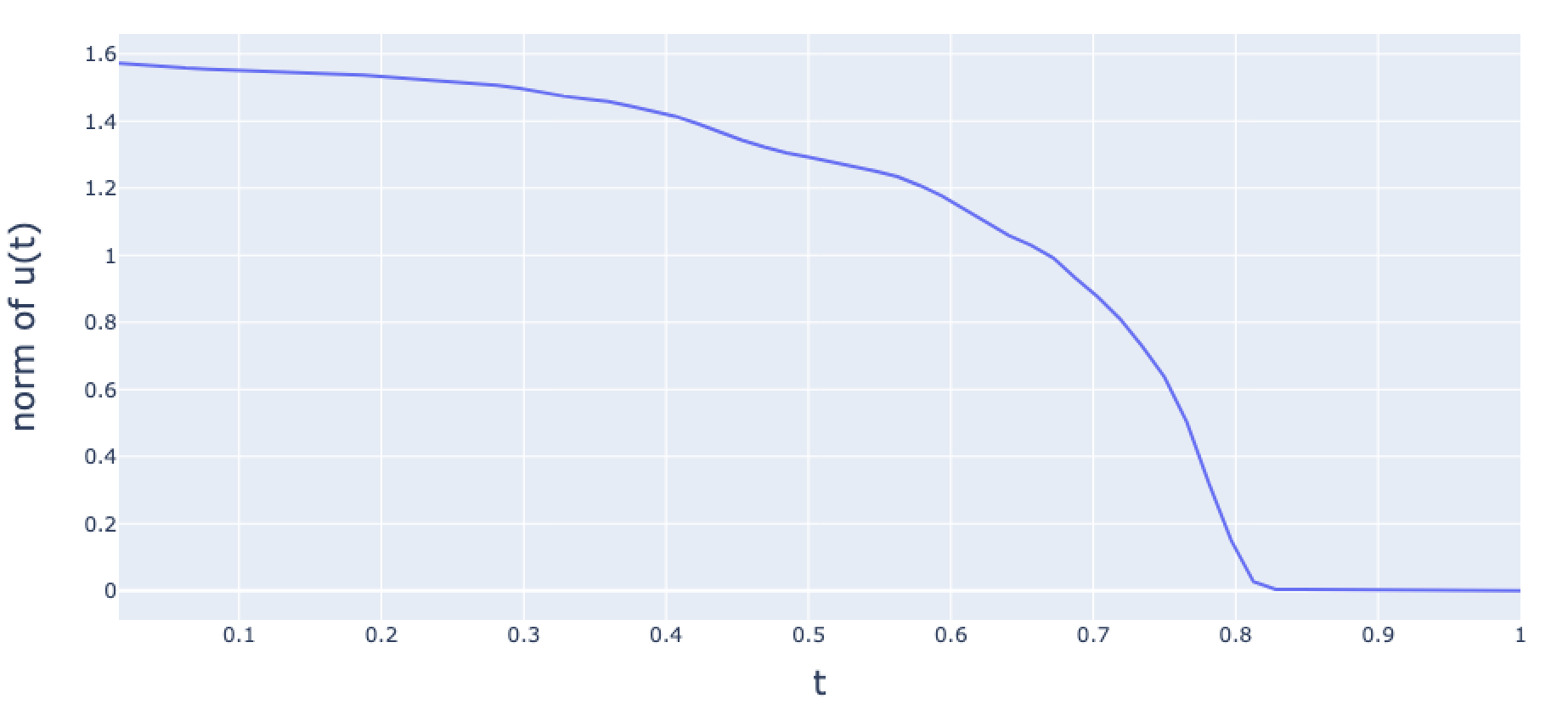
Figure 4. Numerical results for Example 4: sparsity in time.

Figure 5. Numerical results for Example 4: sparsity in space.

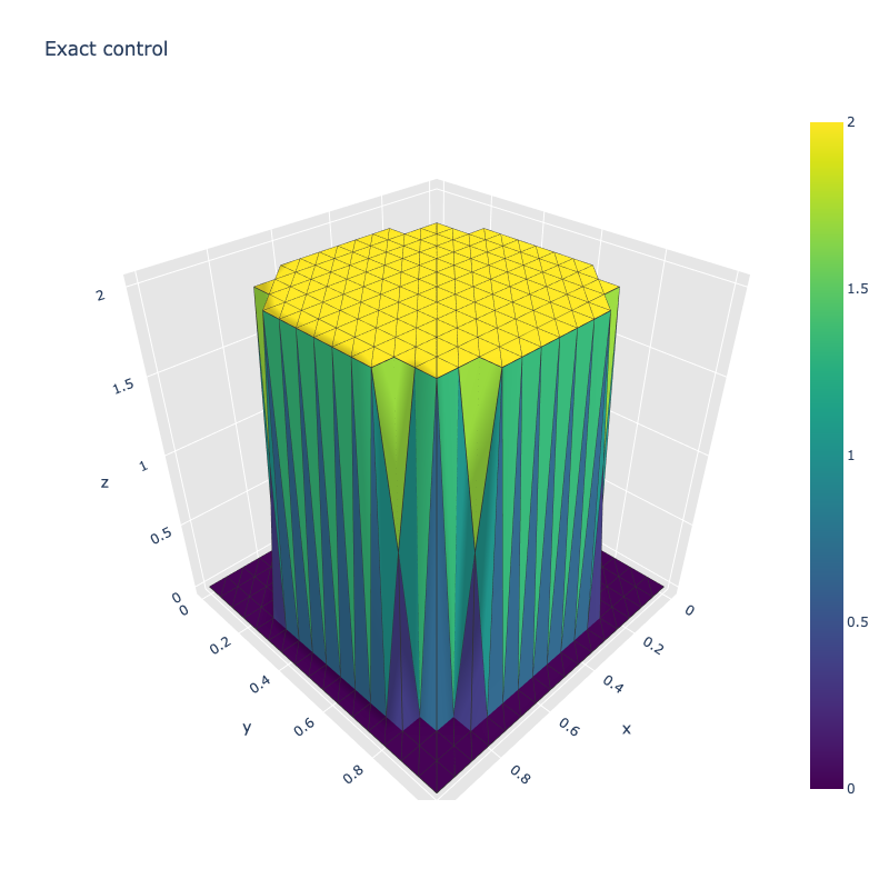
(a) Exact control at $t=0.25$

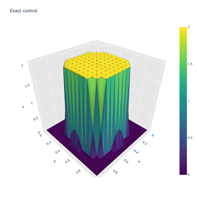
(b) Exact control at $t=0.5$

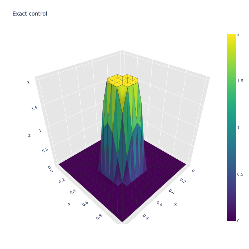
(c) Exact control at $t=0.75$

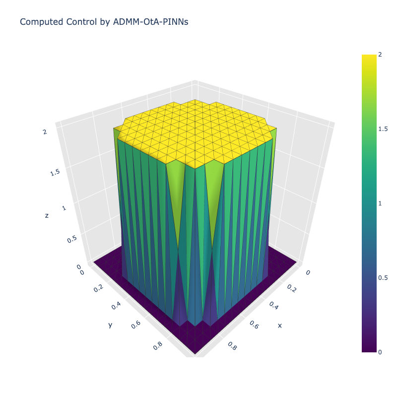
(d) Computed control at $t=0.25$

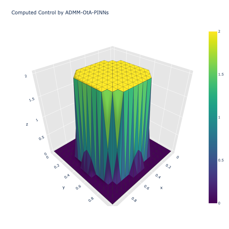
(e) Computed control at $t=0.5$

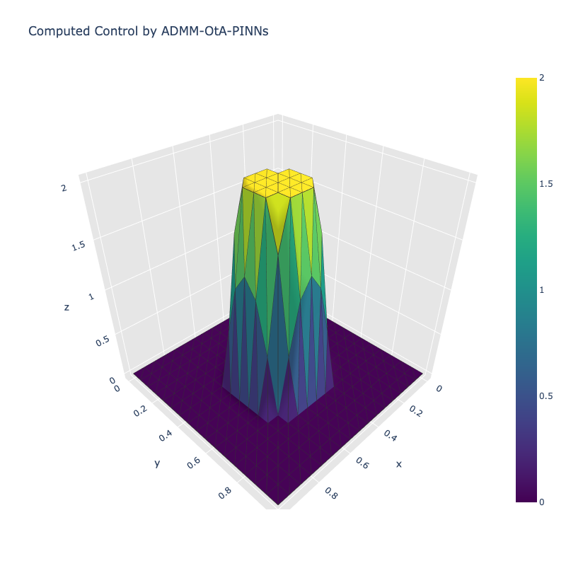
(f) Computed control at $t=0.75$

7. Conclusions and Perspectives

In this paper, we showcased a successful combination of contemporary deep learning techniques with classic operator splitting optimization techniques to design implementable and efficient algorithms for solving challenging PDE-constrained optimization problems. In particular, we suggested enhancing the well-known physics-informed neural networks (PINNs) with the classic alternating direction method of multipliers (ADMM), and thus significantly enlarged the applicable range of the PINNs to nonsmooth cases of PDE-constrained optimization problems. The proposed ADMM-PINNs algorithmic framework can be used to develop efficient algorithms for a class of nonsmooth PDE-constrained optimization problems, including inverse potential problems, source identification in elliptic equations, control constrained optimal control of the Burgers equation, and sparse optimal control of parabolic equations. The resulting algorithms differ from existing algorithms in that they do not require solving PDEs repeatedly and that they are mesh-free, easy to implement, and flexible to different PDEs. We expect the ADMM-PINNs algorithmic framework to pave an avenue of more application-tailored and sophisticated algorithms in the combination of traditional optimization techniques with emerging deep learning developments for solving more challenging problems arising in a broad array of science and engineering fields.

Our work leaves some important questions for future investigation, though solving these questions is beyond the scope of this paper. We list some of them below.

1. A natural extension of this work is to consider other even more challenging PDEs such as the Cahn–Hilliard equation [32], the Navier Stokes equation [31] and the Boussinesq equation [60].

2. The validated efficiency of the ADMM-PINNs algorithms clearly justifies the necessity to investigate the underlying theoretical issues such as the convergence analysis and the error estimate for the proposed algorithmic framework.

3. In our numerical experiments, Algorithm 1 or 2 for solving the $u$-subproblem (2.4) in the ADMM-PINN algorithm framework was terminated empirically. It has been shown in [26] that it is not necessary to pursue a too high-precision solution for (2.4), especially when the iterations are still far from the solution point. Also, solutions with too low precision for (2.4) may not be sufficient to guarantee overall convergence. Therefore, it is important to determine an adaptive inaccuracy criterion to implement the inner PINNs methods to solve (2.4).

4. In Sections 5 and 6, we observed that it is not easy to train the neural networks for the resulting ADMM-AtO-PINNs. A main reason is that the balance between the objective function and the PDE losses is sensitive and unstable. Similar results have also been observed in [29]. To further improve the numerical performance, it seems that some adaptive strategies should be developed for discerning loss weights. Research on this topic seems still to be in infancy.

References

- [1] Alves, C. J., Abdallah, J. B., and Jaoua, M. (2004). Recovery of cracks using a point-source reciprocity gap function. Inverse Problems in Science and Engineering, 12(5), 519-534.
- [2] Baillet, S., Mosher, J. C., and Leahy, R. M. (2001). Electromagnetic brain mapping. IEEE Signal processing magazine, 18(6), 14-30.
- [3] Barry-Straume, J., Sarshar, A., Popov, A. A., and Sandu, A. (2022). Physics-informed neural networks for PDE-constrained optimization and control. arXiv preprint, arXiv:2205.03377.
- [4] Basir, S., and Senocak, I. (2022). Physics and equality constrained artificial neural networks: application to forward and inverse problems with multi-fidelity data fusion. Journal of Computational Physics, 111301.
- [5] Banks, H. T., and Kunisch, K. Estimation Techniques for Distributed Parameter Systems. Springer Science & Business Media, 2012.
- [6] Beck, C., and Jentzen, A. (2019). Machine learning approximation algorithms for high-dimensional fully nonlinear partial differential equations and second-order backward stochastic differential equations. Journal of Nonlinear Science, 29(4), 1563-1619.
- [7] Biccari, U., Song, Y., Yuan, X., and Zuazua, E. (2022). A two-stage numerical approach for the sparse initial source identification of a diffusion-advection equation. arXiv preprint, arXiv:2202.01589.
- [8] Biccari, U., Warma, M., and Zuazua, E. (2021) Control and numerical approximation of fractional diffusion equations. arXiv preprint, arXiv:2105.13671.
- [9] Cai, J. F., Osher, S., and Shen, Z. (2010). Split Bregman methods and frame based image restoration. Multiscale Modeling & Simulation, 8(2), 337-369.
- [10] Chambolle, A. (2004). An algorithm for total variation minimization and applications. Journal of Mathematical Imaging and Vision, 20(1), 89-97.
- [11] Chan, T. F., Golub, G. H., and Mulet, P. (1999). A nonlinear primal-dual method for total variation-based image restoration. SIAM Journal on Scientific Computing, 20(6), 1964-1977.
- [12] Chan, T. F., and Tai, X. C. (2003). Identification of discontinuous coefficients in elliptic problems using total variation regularization. SIAM Journal on Scientific Computing, 25(3), 881-904.
- [13] Chen, Z., and Zou, J. (1999). An augmented Lagrangian method for identifying discontinuous parameters in elliptic systems. SIAM Journal on Control and Optimization, 37(3), 892-910.
- [14] Chiu, P. H., Wong, J. C., Ooi, C., Dao, M. H., and Ong, Y. S. (2022). CAN-PINN: A fast physics-informed neural network based on coupled-automatic–numerical differentiation method. Computer Methods in Applied Mechanics and Engineering, 395, 114909.
- [15] Ciaramella, G., and Borzì, A. (2016). A LONE code for the sparse control of quantum systems. Computer Physics Communications, 200, 312-323.
- [16] Cuomo, S., Di Cola, V. S., Giampaolo, F., Rozza, G., Raissi, M., and Piccialli, F. (2022). Scientific machine learning through physics–informed neural networks: where we are and what’s next. Journal of Scientific Computing, 92, 88.
- [17] Cybenko, G. (1989). Approximation by superpositions of a sigmoidal function. Mathematics of Control, Signals, and Systems, 2 (4), 303–314
- [18] de los Reyes, J. C., and Kunisch, K. (2004). A comparison of algorithms for control constrained optimal control of the Burgers equation. Calcolo, 41(4), 203-225.
- [19] E, W., and Yu, B. (2018). The deep Ritz method: a deep learning-based numerical algorithm for solving variational problems. Communications in Mathematics and Statistics, 6(1), 1-12.
- [20] Faroughi, S. A., Pawar, N., Fernandes, C., Das, S., Kalantari, N. K., and Mahjour, S. K. (2022). Physics-guided, physics-informed, and physics-encoded neural networks in scientific computing. arXiv preprint, arXiv:2211.07377.
- [21] Glowinski, R., and Lions, J. L. (1994). Exact and approximate controllability for distributed parameter systems. Acta Numerica, 3, 269-378.
- [22] Glowinski, R., and Lions, J. L. (1995). Exact and approximate controllability for distributed parameter systems. Acta Numerica, 4, 159-328.
- [23] Glowinski, R., Lions, J. L., and He, J. Exact and Approximate Controllability for Distributed Parameter Systems: A Numerical Approach (Encyclopedia of Mathematics and its Applications), Cambridge University Press, 2008.
- [24] Glowinski, R., and Marroco, A. (1975). Sur l’approximation, par éléments finis d’ordre un, et la résolution, par pénalisation-dualité d’une classe de problèmes de dirichlet non linéaires, Revue française d’automatique, informatique, recherche opérationnelle. Analyse Numérique, 9(R2), 41-76.
- [25] Glowinski, R., Song, Y., and Yuan, X. (2020). An ADMM numerical approach to linear parabolic state constrained optimal control problems. Numerische Mathematik, 144(4), 931-966.
- [26] Glowinski, R., Song, Y., Yuan, X., and Yue, H. (2022). Application of the alternating direction method of multipliers to control constrained parabolic optimal control problems and beyond. Annals of Applied Mathematics, 38(2), 115-158.
- [27] Han, J., Jentzen, A., and E, W. (2018). Solving high-dimensional partial differential equations using deep learning. Proceedings of the National Academy of Sciences, 115(34), 8505-8510.
- [28] Hao, Z., Liu, S., Zhang, Y., Ying, C., Feng, Y., Su, H., and Zhu, J. (2022). Physics-informed machine learning: a survey on problems, methods and applications. arXiv preprint, arXiv:2211.08064.
- [29] Hao, Z., Ying, C., Su, H., Zhu, J., Song, J., and Cheng, Z. (2022). Bi-level physics-informed neural networks for PDE constrained optimization using Broyden’s hypergradients. arXiv preprint arXiv:2209.07075.
- [30] Hestenes, M R. (1969). Multiplier and gradient methods. Journal of Optimization Theory and Applications, 4(5), 303-320.
- [31] Hintermüller, M., and Hinze, M. (2006). A SQP-semismooth Newton-type algorithm applied to control of the instationary Navier–Stokes system subject to control constraints. SIAM Journal on Optimization, 16(4), 1177-1200.
- [32] Hintermüller, M., and Wegner, D. (2012). Distributed optimal control of the Cahn–Hilliard system including the case of a double-obstacle homogeneous free energy density. SIAM Journal on Control and Optimization, 50(1), 388-418.
- [33] Hinze, M., Pinnau, R., Ulbrich, M., and Ulbrich, S. Optimization with PDE Constraints. Springer Science & Business Media, Vol. 23, 2008.
- [34] Hwang, R., Lee, J. Y., Shin, J. Y., and Hwang, H. J. (2021). Solving PDE-constrained control problems using operator learning. arXiv preprint, arXiv:2111.04941.
- [35] Karniadakis, G. E., Kevrekidis, I. G., Lu, L., Perdikaris, P., Wang, S., and Yang, L. (2021). Physics-informed machine learning. Nature Reviews Physics, 3(6), 422-440.
- [36] Kharazmi, E., Zhang, Z., and Karniadakis, G. E. (2019). Variational physics-informed neural networks for solving partial differential equations. arXiv preprint, arXiv:1912.00873.
- [37] Khoo, Y., Lu, J., and Ying, L. (2021). Solving parametric PDE problems with artificial neural networks. European Journal of Applied Mathematics, 32(3), 421-435.
- [38] Kingma, D. P., and Ba, J. Adam: A method for stochastic optimization, in the 3rd International Conference on Learning Representations, 2015; preprint available from https://arxiv.org/ abs/1412.6980
- [39] Kirsch, A. An Introduction to the Mathematical Theory of Inverse Problems. New York: Springer, 2011.
- [40] Jiao, Y., Jin, Q., Lu, X., and Wang, W. (2016). Alternating direction method of multipliers for linear inverse problems. SIAM Journal on Numerical Analysis, 54 (4), 2114-2137.
- [41] Lagaris, I. E., Likas, A., and Fotiadis, D. I. (1998). Artificial neural networks for solving ordinary and partial differential equations. IEEE Transactions on Neural Networks 9(5), 987–1000.
- [42] Lance, G., Trélat, E., and Zuazua, E. (2022). Numerical issues and turnpike phenomenon in optimal shape design. Optimization and control for partial differential equations: Uncertainty quantification, open and closed-loop control, and shape optimization, 29: 343.
- [43] Lions, J. L. Optimal Control of Systems Governed by Partial Differential Equations (Grundlehren der Mathematischen Wissenschaften), vol. 170, Springer Berlin, 1971.
- [44] Lu, L., Meng, X., Mao, Z., and Karniadakis, G. E. (2021). DeepXDE: A deep learning library for solving differential equations. SIAM Review, 63(1), 208-228.
- [45] Lu, L., Pestourie, R., Yao, W., Wang, Z., Verdugo, F., and Johnson, S. G. (2021). Physics-informed neural networks with hard constraints for inverse design. SIAM Journal on Scientific Computing, 43(6), B1105-B1132.
- [46] Lye, K. O., Mishra, S., Ray, D., and Chandrashekar, P. (2021). Iterative surrogate model optimization (ISMO): an active learning algorithm for PDE constrained optimization with deep neural networks. Computer Methods in Applied Mechanics and Engineering, 374, 113575.
- [47] Mitusch, S. K., Funke, S. W., and Kuchta, M. (2021). Hybrid FEM-NN models: Combining artificial neural networks with the finite element method. Journal of Computational Physics, 446, 110651.
- [48] Mowlavi, S., and Nabi, S. (2023). Optimal control of PDEs using physics-informed neural networks. Journal of Computational Physics, 473, 111731.
- [49] Nocedal, J. (1980). Updating quasi-Newton matrices with limited storage, Mathematics of Computation, 35(151), 773-782.
- [50] Pakravan, S., Mistani, P. A., Aragon-Calvo, M. A., and Gibou, F. (2021). Solving inverse-PDE problems with physics-aware neural networks. Journal of Computational Physics 440, 110414.
- [51] Powell, M. J. D. (1969). A method for nonlinear constraints in minimization problems, in Optimization, R. Fletcher, ed., Academic Press, New York, 283-298.
- [52] Psichogios, D. C., and Ungar, L. H. (1992). A hybrid neural network‐first principles approach to process modeling. AIChE Journal, 38(10), 1499-1511.
- [53] Raghu, M., Poole, B., Kleinberg, J., Ganguli, S., and Sohl-Dickstein, J. (2017). On the expressive power of deep neural networks. In International Conference on Machine Learning, 2847-2854
- [54] Raissi, M., Perdikaris, P., and Karniadakis, G. E. (2019). Physics-informed neural networks: A deep learning framework for solving forward and inverse problems involving nonlinear partial differential equations. Journal of Computational physics, 378, 686-707.
- [55] Rudin, L. I., Osher, S., and Fatemi, E. (1992). Nonlinear total variation based noise removal algorithms. Physica D: Nonlinear Phenomena, 60(1-4), 259-268.
- [56] Schindele, A., and Borzì, A. (2017). Proximal schemes for parabolic optimal control problems with sparsity promoting cost functionals, International Journal of Control, 90, 2349-2367.
- [57] Stadler, G. (2009). Elliptic optimal control problems with -control cost and applications for the placement of control devices. Computational Optimization and Applications, 44(2), 159-181.
- [58] Sirignano, J., and Spiliopoulos, K. (2018). DGM: A deep learning algorithm for solving partial differential equations. Journal of Computational Physics, 375, 1339-1364.
- [59] Song, Y., Yuan, X., and Yue, H. (2019). An inexact Uzawa algorithmic framework for nonlinear saddle point problems with applications to elliptic optimal control problem. SIAM Journal on Numerical Analysis, 57(6), 2656-2684.
- [60] Song, Y., Yuan, X., and Yue, H. (2022). A numerical approach to the optimal control of thermally convective flows. arXiv preprint arXiv:2211.15302.
- [61] Sun, Y., Sengupta, U., and Juniper, M. (2022). Physics-informed deep learning for simultaneous surrogate modelling and PDE-constrained optimization. Bulletin of the American Physical Society.
- [62] Tarantola, A. Inverse Problem Theory and Methods for Model Parameter Estimation, SIAM: Philadelphia, 2005
- [63] Tian, W., Yuan, X., and Yue, H. (2021). An ADMM-Newton-CNN numerical approach to a TV model for identifying discontinuous diffusion coefficients in elliptic equations: convex case with gradient observations. Inverse Problems, 37(8), 085004.
- [64] Tröltzsch, F. Optimal Control of Partial Differential Equations: Theory, Methods, and Applications, Vol. 112, AMS, 2010.
- [65] Volkwein, S. Mesh-independence of an augmented Lagrangian-SQP method in Hilbert spaces and control problems for the Burgers equation, Doctoral dissertation, Technische Universität Berlin, 1997.
- [66] Volkwein, S. (2001). Distributed control problems for the Burgers equation, Computational Optimization and Applications, 18(2), 115-140.
- [67] Wachsmuth, G., and Wachsmuth, D. (2011). Convergence and regularization results for optimal control problems with sparsity functional. ESAIM: Control, Optimisation and Calculus of Variations, 17(3), 858-886.
- [68] Wang, S., Bhouri, M. A., and Perdikaris, P. (2021). Fast PDE-constrained optimization via self-supervised operator learning. arXiv preprint arXiv:2110.13297.
- [69] Wang, D., Kirby, R. M., MacLeod, R. S., and Johnson, C. R. (2013). Inverse electrocardiographic source localization of ischemia: an optimization framework and finite element solution. Journal of Computational Physics, 250, 403-424.
- [70] Wang, S., Wang, H., and Perdikaris, P. (2021). Learning the solution operator of parametric partial differential equations with physics-informed DeepONets. Science Advances, 7(40), eabi8605.
- [71] Xu, K., and Darve, E. (2022). Physics constrained learning for data-driven inverse modeling from sparse observations. Journal of Computational Physics, 453, 110938.
- [72] Yu, J., Lu, L., Meng, X., and Karniadakis, G. E. (2022). Gradient-enhanced physics-informed neural networks for forward and inverse PDE problems. Computer Methods in Applied Mechanics and Engineering, 393, 114823.
- [73] Xue, T., Beatson, A., Adriaenssens, S., and Adams, R. (2020). Amortized finite element analysis for fast PDE-constrained optimization. In International Conference on Machine Learning, PMLR, 10638-10647.
- [74] Zhang, K., Zuo, W., Chen, Y., Meng, D., and Zhang, L. (2017). Beyond a Gaussian denoiser: Residual learning of deep cnn for image denoising. IEEE Transactions on Image Processing, 26(7), 3142-3155.
- [75] Zhu, Y., Zabaras, N., Koutsourelakis, P. S., and Perdikaris, P. (2019). Physics-constrained deep learning for high-dimensional surrogate modeling and uncertainty quantification without labeled data. Journal of Computational Physics, 394, 56-81.
- [76] Ziemer, W. P. Weakly Differentiable Functions: Sobolev Spaces and Functions of Bounded Variation, Springer-Verlag, New York, 1989.