Navya3DSeg - Navya 3D Semantic Segmentation
Dataset Design & split generation for autonomous vehicles

Abstract

Autonomous driving (AD) perception today relies heavily on deep learning based architectures requiring large scale annotated datasets with their associated costs for curation and annotation. The 3D semantic data are useful for core perception tasks such as obstacle detection and ego-vehicle localization. We propose a new dataset, Navya 3D Segmentation (Navya3DSeg), with a diverse label space corresponding to a large scale production grade operational domain, including rural, urban, industrial sites and universities from 13 countries. It contains 23 labeled sequences and 25 supplementary sequences without labels, designed to explore self-supervised and semi-supervised semantic segmentation benchmarks on point clouds. We also propose a novel method for sequential dataset split generation based on iterative multi-label stratification, and demonstrated to achieve a +1.2% mIoU improvement over the original split proposed by SemanticKITTI dataset. A complete benchmark for semantic segmentation task was performed, with state of the art methods. Finally, we demonstrate an Active Learning (AL) based dataset distillation framework. We introduce a novel heuristic-free sampling method called ego-pose distance based sampling in the context of AL. A detailed presentation on the dataset is available here https://www.youtube.com/watch?v=5m6ALIs-s20.

I INTRODUCTION

Large scale semantic segmentation of point clouds has received lots of attention due to their utility in modern autonomous driving perception systems for creation of HDMaps, ground truth generation (3D detection, panoptic segmentation) and automated labeling systems, robustifying localization modules for Autonomous Vehicles (AV), road surface reconstruction and model fitting [1]. Several models dedicated to semantic segmentation task have been proposed to work on LiDAR data [2] [3] [4] [5] and some with multi-modality and images data like [6], which achieve impressive results. All rely on large scale datasets, such as SemanticKITTI [7], nuScenes [8] [9] or Waymo Open Dataset [10]. Building perception datasets is resource intensive, requiring dedicated acquisition vehicles, post-process data pipeline and annotation platforms, making entry into production a high initial cost.

We propose the following contributions in this paper:

• Navya3DSeg (Fig. LABEL:fig:n3ds_samples) is a high diversity autonomous vehicle dataset built for semantic segmentation task. It was constructed with an affordable LiDAR containing over 50,000 labeled and 80,000 unlabeled frames coming from over 13 countries, 39 cities and 3 continents. Navya3DSeg is, to our knowledge, the most diverse and representative of real AV operation dataset released to this date. The point clouds were batch annotated with temporal consistency to provide precise labeling over 30 labels grouped into 6 categories. The semantic label definition on point clouds is a critical step in constructing datasets. We have included the CURB label to our point cloud dataset (frequently omitted for LiDAR in AV datasets) to enable perception tasks such as lateral localization, lane fitting and road segmentation.

• A novel implementation of multi-label stratified dataset split for sequential LiDAR scan data to obtain better train, validation and test subsets. We demonstrate an improved train-validation split on the existing SemanticKITTI dataset with an improved test set performance in mIoU of 1.2% over the baseline split provided.

• An extensive benchmark of semantic segmentation on existing state of the art models, SqueezeSegV2 [4], SalsaNext [3] and Cylinder3D [2].

• A Bayesian Active Learning (AL) benchmark to perform dataset distillation on Navya3DSeg.

• A novel ego-pose distance based, heuristic-free sampling method for sequential datasets.

II Related work

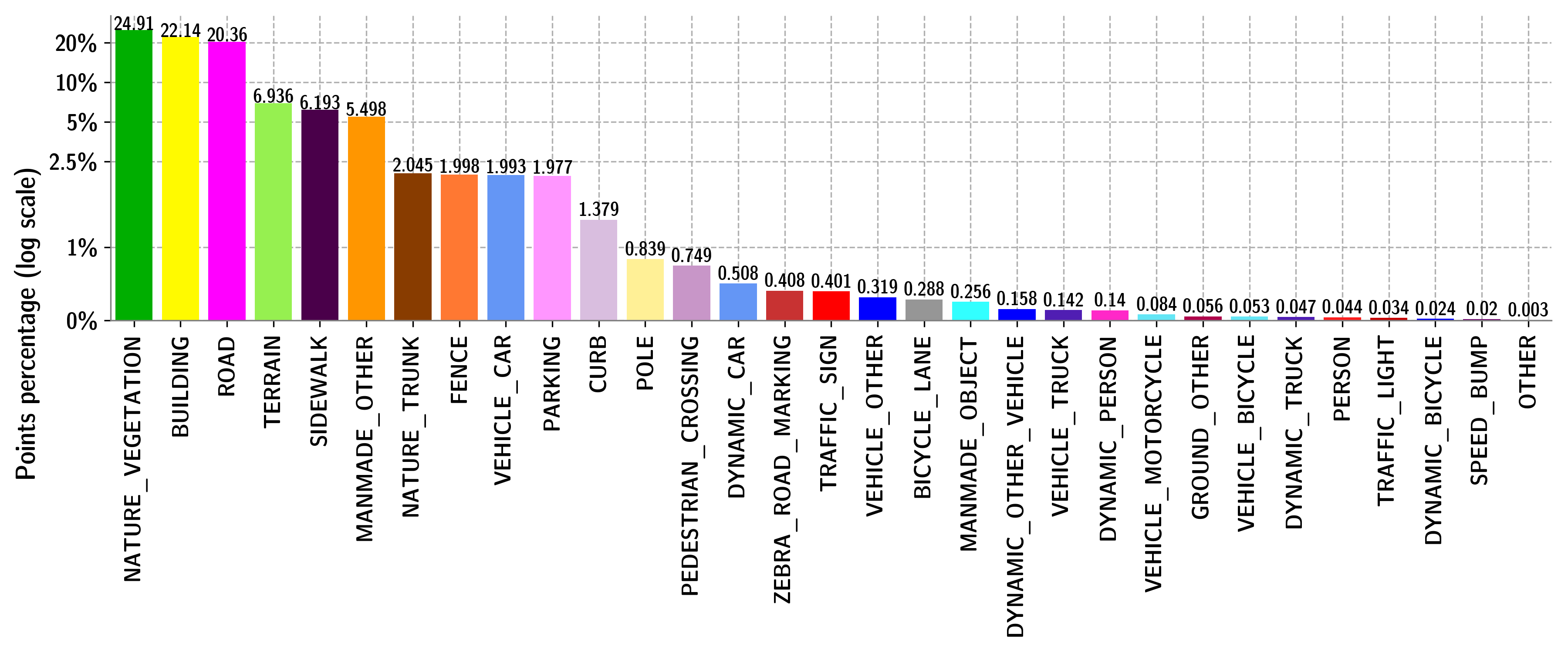
Figure 1: Label distribution of Navya3DSeg.

Advances in LiDAR perception and point cloud related tasks have created a new wave of autonomous driving datasets. A pioneer in the field was SemanticKITTI [7], a dataset with semantic labels for 3D point clouds generated from a Velodyne HDL-64E LiDAR. Waymo releases Waymo Open Dataset (WOD) [10], a perception dataset with 2D and 3D semantic annotations, 2D and 3D instance bounding boxes, with sequences recorded only in the USA. Unfortunately, the sensor set is proprietary (composed of 1 long range and 4 mid range LiDARs), and the annotations on point clouds were obtained after 2D-3D re-projection from camera. Thus, 3D semantic labels are provided for a small fraction of the dataset, and only for their long range LiDAR, at a frequency of 2Hz. Thus the 3D labels are not temporally consistent and do not permit frame aggregation during model training. Motional [8] proposed the first 3D multi-modal object detection dataset, recorded in the cities of Boston and Singapore, using a Velodyne HDL-32E LiDAR, with an extension called Panoptic nuScenes [9], while SemanticPOSS [11] dataset focuses on dynamic labels. Finally, KITTI-360 dataset [12] contains semantic segmentation and bounding box annotations in both image and LiDAR modalities (Velodyne HDL-64E and a SICK LMS 200 laser). A recent point cloud semantic segmentation dataset, HelixNet, using a Velodyne HDL-64E LiDAR, focusing mainly on french locations was released by [13]. Table I compares Navya3DSeg to the aforementioned datasets.

Point cloud datasets are key for autonomous driving perception tasks, and among them we can cite:

• Semantic Occupancy Grid & Bird Eye View (BEV) Perception: A Semantic Occupancy Grid (SOG) is a discrete 2D-cell representation of space with an associated label. SOG and BEV representations are key to perform multi-sensor fusion and upstream usage by tracking, path planning and decision making modules [14].

• Automating HDMap creation: Semantic point clouds are useful in automating various sub-tasks in HDMaps creation: lane, curbs, road edge and topology extraction, depth and elevation map extraction [1]. Semantic point clouds also help improve global localization [15].

TABLE I: Dataset comparison

Name	# labeled scans	LiDAR sensor set	Countries	Labels
SemanticKITTI	43552	Velodyne HDL-64E	1 (Germany)	28
SemanticPOSS	2988	Hesai Pandora	1 (China)	14
KITTI-360	100000	Velodyne HDL-64E	1 (Germany)	19
nuScenes	40000	Velodyne HDL-32E	2 (USA, SG)	32
Waymo Open Dataset	46000	1 in-house LiDAR	1 (USA)	23
Navya3DSeg	50070	Hesai Pandar40	9	30

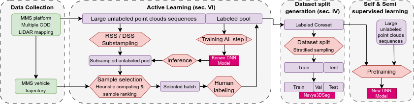
Figure 2: An overview of the data collection, AL coreset extraction with human in the loop, and dataset splitting steps.

III Navya3DSeg dataset

Navya’s autonomous shuttle operates on a varied operational domain, including rural, urban, coastal and industrial sites. The Navya3DSeg dataset was designed for autonomous shuttles operating in these special environments. It was created with an affordable but production grade mapping system, which is modular and usable with any vehicle. The Navya3DSeg dataset was built for the task of 3D semantic segmentation to automate the task of semantic 3D maps generation.

Dataset size and diversity: Navya3DSeg is split into a labeled and an unlabeled part. The labeled part is made of carefully selected 23 sequences from 9 countries (Japan, China, Norway, Denmark, Germany, Switzerland, France, Israel, USA), over 20 different cities, for a total of more than 1.5 billion points. The unlabeled part contains 25 sequences from 8 countries (Japan, South Korea, France, Norway, Saudi Arabia, UAE, USA, Scotland) and 20 cities, for a total amount of more than 2.5 billion points. With an accumulated path length of more than 130 kilometers, the sequences were collected across various environments that include urban, country side and residential areas, but also scenes with multi-lanes roads, roundabouts, intersections with cars, trucks, pedestrians in traffic, etc.

Hardware and sensors setup for dataset acquisition: Navya3DSeg point clouds were collected using Navya’s in-house mapping platform, called Mobile Mapping System (MMS). It hosts an affordable single LiDAR sensor, a Hesai Pandar40 with 40 layers, a vertical and horizontal field of view of 23° (-16° to 7°) and 360°, and a vertical and horizontal angular resolution of 0.33° and 0.4°. On MMS, the LiDAR has an orientation of 15° towards the ground. This pitch provides a focus on the ground and reduces samples of dynamic objects in front of the ego vehicle, which is essential to build maps for localization purpose. An iXblue ATLANS-C Inertial Navigation System (INS) provides high precision position and orientation data, leading to registered point clouds without any explicit SLAM or registration algorithms.

Labels: The human expert based annotation was conducted jointly with Playment, Telus International. The annotation pipelines for autonomous perception were well established, with several verification steps to evaluate the quality of annotations. We associate 25 static and 5 dynamic labels to each point in the Navya3DSeg dataset. These 30 labels are grouped into 6 categories: Ground, Vehicle, Manmade, Human, Nature and Dynamic. Navya3DSeg contains (see Fig. 1) a large amount of label imbalance due to the natural distribution between objects and features observed in the real world, notably, the frequency of 20 different labels is less than 1% of the dataset. Navya3DSeg dataset introduces the CURB label which is missing in most large scale semantic segmentation datasets. Bei et al. [16] highlight the lack of a dedicated CURB label in point cloud datasets, and discuss classical processing methods to extract them at a large scale. The CURB label represents 1.379% of Navya3DSeg, namely 21,45 million points coming from various environments, from national road to urban areas, including some complex cases like crossroad and driveways which are useful for HDMap and road map generation.

Dataset design and benchmarking: Dataset extension with AL [17] has been important in industrial research, where the goal of a dataset is to provide a diversified and comprehensive large-scale ground truth for point cloud semantic segmentation task. We focus on equally important problems of dataset extension and coreset selection with AL. This enables us to extend existing datasets over time while reducing redundancy and improve model performance. We demonstrate ego-vehicle trajectory based sampling and model uncertainty driven data collection policies. Finally at the end of this pipeline we apply dataset splitting to create train, validation and test subsets. The Navya3DSeg’s unlabeled pool is provided for baseline pre-training experiments on semi and self-supervised tasks, that could enable improvement over the primary semantic segmentation task performance on the original labeled coreset, see Fig. 2.

IV Dataset split generation

Splitting datasets is a key hidden engineering step for dataset construction through the direct impact on model’s capacity to generalize. Dataset splitting partitions a large dataset into train, validation and test subsets. The split should ensure a training subset with large diversity to fit large models, a validation subset to fit hyper-parameters for model selection, and finally a test subset to evaluate the generalization performance of the optimal (on validation subset) model. Concretely, stratification is employed for dataset splits. Stratified splits are defined as k-way partitions of full dataset such that the joint distribution of the labels is conserved, while respecting the subset target ratios. Most stratified algorithms preserve the unitary label frequency, especially to avoid rare joint label redistribution cases. Sechidis et al. [18] propose Multi-label Stratified Shuffle Split (MSSS), where each sample is associated with multiple labels, operating on label-indicator function per sample, without their numerical frequency. Higher order interactions between labels were studied in [19]. Yogamani et al. [20] presented the Woodscape dataset and were one of the firsts to address this problem on fish-eye perception dataset, and applied a stratified dataset split strategy. They also provide multiple splits to achieve consistent hypothesis evaluation.

All consequent analysis, benchmarks and iterations on the model are influenced by this split. As Uricar et al. [21] mention, one of the key problem in using traditional random sampling based splits is the manifestation of law of small numbers leading to bias in creating the splits. One single instance of random sampling does not ensure a good label distribution in the subsets. This is comparable to get a different proportion of heads with a small number of flips of an unbiased coin. As one increases the number of flips, the frequency of getting heads or tail reaches the expected value of 0.5 gradually. A poor choice in splits leads to significant label imbalance issue between the training and validation subsets. SemanticKITTI has 98% of bicycle label points in validation set (sequence 08) and the rest in the training set. We demonstrate a case study in subsection IV-C.

We repeat definitions from [18] of metrics to evaluate the quality of generated splits.

1. Label Distribution (LD) (eq. 1) evaluates the divergence between the class-distribution in a subset of the split to the class-distribution of the whole dataset, for $c$-classes. Given the dataset $D$, the $k$-subsets : $S_{1},...,S_{k}$:

   $$LD=\frac{1}{c}\sum_{i=1}^{c}(\frac{1}{k}\sum_{j=1}^{k}|\frac{|S_{j}^{i}|}{|S_{j}|-|S_{j}^{i}|}-\frac{|D^{i}|}{|D|-|D^{i}|}|)$$ (1)

   where $c$ is the number of labels, $D^{i}$ is the number of samples containing label $i$, $S_{j}^{i}$ is the number of samples in subset $S_{j}$ containing label $i$. We propose here an extension of LD, inverse frequency weighted label distribution (IFWLD, eq.2), which emphasizes the impact of critical labels, the main cause of label distribution shift among split subsets.

   $$IFWLD=\sum_{i=1}^{c}\frac{|D|}{D_{i}}(\frac{1}{k}\sum_{j=1}^{k}|\frac{|S_{j}^{i}|}{|S_{j}|-|S_{j}^{i}|}-\frac{|D^{i}|}{|D|-|D^{i}|}|)$$ (2)

2. We propose an input domain sensitive metric, Intensity Drift Score (IDS). It is calculated as the average Wasserstein distance (WD) between sample distributions of intensity channel values. We used Deepchecks library [22], which implements WD from Scipy [23].

3. Examples Distribution (ED) [18] measures how the target subset size $\left|S_{j}\right|$ deviates from the desired ratio $c_{j}$ over the full dataset : $ED=\frac{1}{k}\sum_{j=1}^{k}\lvert\lvert S_{j}\rvert-c_{j}\rvert$. Our desired subset ratio in our experiments train:validation:test is 0.7:0.1:0.2.

4. Label Kullback-Leibler Divergence (KL) : We measure the average (over 3 subsets) KL-divergence between normalized K-class histogram $P$ for subsets, and $Q$ for full dataset . $KL(P||Q)=\sum_{c\in[1,K]}p(k)\log(\frac{p(k)}{q(k)})$, where $p(c),q(c)$ refers to probability of class $c$ in subset and dataset respectively.

IV-A Stratified Sampling for Sequences

Stratified sampling is usually achieved by proportionate allocation of labels between subsets. This is seen as a greedy optimization problem. In a classification problem with single label’s per image, one could employ stratified sampling from Scikit-learn [24]. In case of object detection and segmentation, each sample is associated with multiple labels, referred to as multi-label/label-set classification problems. Sechidis et al. [18] introduce Multi-label Stratified Shuffle Split (MSSS) as solution for the binary multi-label case stratification problem. Since we work on point cloud sequences, we generalize the single sample based MSSS to sequential data by considering concatenation of consecutive scans as a single sample. This helps reduce temporal correlation between subsets. We shall term the size of this grouping to be the granularity parameter. Furthermore in our extension, termed as Multi-label Segment Stratified Shuffle Split (MSegSSS), we use the actual frequency of labels in each segment of grouped scans, where as MSSS considers just the binary presence/absence of labels. In standard MSSS implementation, Sechidis et al. [18] iteratively assign samples based on label frequency (going from least to most frequent) to the different k-splits. While in our method, due to the effect of aggregation of samples into larger segments, several labels land-up with similar frequencies, we choose the least present sequence associated with samples to assign to splits in such a case. Smaller granularity segments produces smaller input-output domain divergence between subset and dataset. When working with complete sequences of variable size, granularity is variable, an advantage of the MSegSSS algorithm.

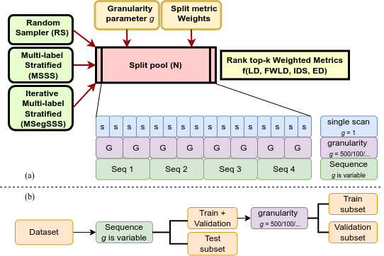
Figure 3: (a): Split module with granularity. (b): Train, Validation and Test subsets creation pipeline.

Sampling methods: Our split module (Fig. 3) contains three sampling methods to generate a split, which are Random, MSSS and MSegSSS. The Navya3DSeg test set, representing our target domain, was built with a sequence level granularity, meaning that each subset is composed of complete sequences. The test set will remain fixed, though different train/validation subsets can be generated at different granularity.

Split procedure: We use the aforementioned methods to generate a pool of multiple splits. The splits are ranked by the final objective function evaluated by the weighted combination of split metrics (LD, FWLD, IDS, ED). The selected split is the one on top of the ranking table, closest to the combination of our objectives. Navya3DSeg default split is generated by following this procedure with granularity as sequence size.

When compared to SemanticKITTI dataset split, the selected split of Navya3DSeg generated by our split module has lower values of IDS and LD, as shown in table II, thanks to the use of stratification for split creation for Navya3DSeg.

TABLE II: Metrics results from the dataset split module

Dataset	LD (train, validation )	IDS (train, validation, test)
Navya3DSeg	0.00512	0.005861
SemanticKITTI	0.00809	0.049727

IV-B Sampling methods evaluation

We performed a benchmark of sampling methods for dataset split creation of train and validation subsets, with different granularity levels. For this, we generate 10000 different splits with a desired ratio of 0.8:0.2 (train:validation) for each sampling method and granularity level selected, and evaluate them by our split metrics. From table III, MSegSSS is the best method overall to sample a split satisfying the condition of label distribution. MSegSSS is slightly better than MSSS, based on LD and IFWLD. Both MSSS and MSegSSS are better than Random in all metrics. However, MSSS and MSegSSS are computationally more expensive than Random, especially MSegSSS. Thus, choosing the optimal sampling method depends on the available computation power and the objectives. In practice, MSegSSS ensures a good split with few instances of splits in the pool, while MSSS and Random could bring similar splits, as the number of instances in the pool becomes very large.

TABLE III: Navya3DSeg sampling method benchmark for dataset split creation for training and validation subsets

Granularity	Method	mean(LD)	mean(IFWLD)	mean(IDS)	mean(ED)
100	MSSS	2,4031E-03	9,5066E-06	2,0470E-03	2,3920E-02
	MSegSSS	2,3944E-03	9,5048E-06	2,0505E-03	2,3921E-02
	RANDOM	2,6614E-03	1,0546E-05	2,6401E-03	2,6157E-02
500	MSSS	4,5246E-03	1,6637E-05	7,0008E-03	4,2733E-02
	MSegSSS	4,5031E-03	1,6629E-05	7,0315E-03	4,2695E-02
	RANDOM	5,0154E-03	1,7803E-05	8,1847E-03	4,4778E-02
2000	MSSS	8,2665E-03	2,7897E-05	1,6546E-02	7,4636E-02
	MSegSSS	8,2336E-03	2,7858E-05	1,6425E-02	7,4666E-02
	RANDOM	8,4730E-03	2,8399E-05	1,7790E-02	7,6469E-02

IV-C Granularity evaluation

To evaluate the effect of granularity, we use our split module (Fig. 3) to generate train/validation splits with different granularity values, then evaluate them using our split metrics (LD, IDS) and mIoU metrics on test set. We chose SalsaNext as the training architecture and the best model weights are selected based on mIoU evaluated on validation set for each split. The table IV shows experiments on different train/validation splits, corresponding to different granularity, and evaluated on the same test set of each dataset.

Navya3DSeg: Smaller granularity results in artificially high performance scores on both train and validation subsets. The worst case is granularity of 1. This is due to the temporal correlation between scans in training and validation sets, and leads to subsequent poor test set generalization. The ideal split extraction is a constrained optimization problem, which minimizes temporal correlation between subsets, as well as minimizes split metrics for given granularity. The higher the granularity, the lower the temporal correlation between subsets, but at the same time, splits might not reach the target ratios for subset size. For both SemanticKITTI and Navya3DSeg, the test subset is made with a split at sequence level. But for Navya3DSeg, it is defined with stratification.

In Table IV, we obtain two splits with the same granularity of 2000, but with different obtained subset size ratios (different from the targeted ratios, since obtained ratio achieved is output sensitive). The $2000^{\dagger}$ granularity split with targeted ratio aligned with sequence level split, has higher scores on validation and lower on test, with lower KL divergence, with small loss in IDS scores. While the 2000 granularity split shows that the algorithm can produce obtained split ratios not respecting the input targeted ratios, leading to poorer performances across metrics.

SemanticKITTI original dataset split is imbalanced with a validation set (sequence 08) being the dataset’s most diverse and longest sequence. Especially, it contains 99.2% of static bicyclists labels in the dataset. There are high intensity drift between validation and train sets, and also between validation and test sets. We take advantage of our split module to find another train/validation split with lower label divergence and intensity shift, while having similar sizes of train and validation sets. As a result, the models trained on splits with granularity of 500 and 1000 have better performance on test set compared to the one trained on the default split, with a 1.2% mIoU boost when granularity is set to 500.

TABLE IV: Granularity evaluation on Navya3DSeg and SemanticKITTI. The sequence split (Sequence*) of SemanticKITTI was taken from the dataset configuration

Dataset	Input variables		Output metrics
	Granularity	Targeted ratios	Obtained ratios	LD $\downarrow$	IDS $\downarrow$	KL Divergence $\downarrow$	Train mIoU	Val mIoU	Test mIoU
Navya3DSeg	Sequence	87.5:12.5	79.8:20.2	5,10E-03	5,90E-03	6,45E-03	73.15	45.67	50.69
	2000	87.5:12.5	87.3:12.7	4,60E-03	1,80E-02	7,01E-03	69.03	47.27	48.30
	$2000^{\dagger}$	79.8:20.2	79.5:20.5	4,30E-03	6,00E-03	4,27E-03	72.05	47.93	49.37
	500	79.8:20.2	79.0:21.0	4,70E-03	3,60E-03	1,62E-03	72.77	54.59	50.49
	1	79.8:20.2	79.7:20.3	2,00E-04	1,00E-04	7,00E-06	72.10	72.72	51.09
SemanticKITTI	Sequence*	-	82.7:17.3	8,10E-03	6,53E-02	1,87E-02	80.84	53.66	54.81
	1000	82.7:17.3	82.0:18.0	6,80E-03	3,50E-03	1,31E-02	81.62	61.43	56.00
	500	82.7:17.3	82.5:17.5	3,40E-03	2,70E-03	4,35E-03	82.47	64.03	55.97

V Semantic segmentation benchmark

V-A Navya3DSeg semantic segmentation benchmark

Several labels have a very low frequency in Navya3DSeg (Fig. 1); this is why we employ a label mapping to group certain labels into one single label to get a more balanced label distribution over the dataset. As an example, the label BICYCLE_LANE is mapped to ROAD. This label mapping is used in experiments at sections IV, V and VI. We present here the benchmark results on the semantic segmentation task, using range image based representation network architectures such as SalsaNext [3], SqueezeSegV2 [4], and 3D cylindrical based representation network Cylinder3D [2], which takes advantage of the full 3D sparsity of the point clouds. For range image based representation networks, we apply a spherical projection [4] on point clouds to obtain 2D range images with a resolution of 896x40 (SqueezeSegV2) and 900x40 (SalsaNext) as inputs for the network. With Cylinder3D, we use the default cylindrical grid configuration of size [480, 360, 32] to build the cylindrical partition which keeps an uniform point distribution within voxels across distance. Cylinder3D is the most effective architecture, as seen on table V. It is noted that Navya3DSeg default split (section IV) is used for all experiments in sections V and VI.

In order to evaluate Navya3DSeg on different architectures, we use standard metrics for semantic segmentation tasks, namely Intersection over Union (IoU), Precision-Recall and F1-Scores. Following Fong et al. [9], for each metric we also compute the mean and frequency weighted average over every label for each set (validation, test) and subset (things, stuff).

TABLE V: label IoU: baseline models evaluated on test set

	mIoU	fwIoU	BICYCLE	BUILDING	CAR	CURB	FENCE	MANMADE_OBJECT	MANMADE_OTHER	MOTORCYCLE	PARKING	PERSON	POLE	ROAD	SIDEWALK	TERRAIN	TRAFFIC_LIGHT	TRAFFIC_SIGN	TRUCK	TRUNK	VEGETATION	VEHICLE_OTHER
SqueezeSegV2	41.46	60.89	37.07	81.23	70.65	43.22	22.3	7.77	31.77	58.36	12.08	30.83	27.44	85.79	57.52	54.3	8.92	34.1	3.11	26.09	69.07	26.24
SalsaNext	53.35	70.88	48.08	84.7	76.27	51.24	35.4	23.74	42.75	71.43	19.53	57.34	46.96	88.04	65.55	64.83	28.15	43.46	6.92	40.47	77.84	41.04
Cylinder3D	62.84	81.16	67.39	92.26	89.51	53.60	55.24	36.01	50.35	88.32	25.96	79.12	63.36	89.62	69.74	68.27	49.66	55.10	36.84	53.08	84.14	49.21

V-B Cross-dataset experiments

Here we evaluate fine-tuning between SemanticKITTI and Navya3DSeg. The experiment results are reported on validation set after 3D point cloud reprojection with SalsaNext architecture. There is a significant domain gap between SemanticKITTI and Navya3DSeg, mainly due to:

• Sensor intrinsics: Navya3DSeg has been acquired from a Hesai Pandar40 LiDAR while SemanticKITTI team used a Velodyne HDL-64E. These two sensors have a different number of layers, vertical Field of View (vFoV), angular resolution and intensity distribution. It results in different range-image representations.

• Sensor extrinsics: Navya3DSeg LiDAR sensor is oriented with a pitch of 15° towards the ground while that of SemanticKITTI is laid flat at 0°. Objects in front and back of the vehicles sample different classes (buldings, roads, vegetation) differently, leading to a domain shift.

• Annotation policy: There are common labels between both datasets, nevertheless, the annotation policy for each label may differ from a dataset to another.

• Acquisition conditions: Most of Navya3DSeg acquisitions were done by night, thus dynamic labels spatial distribution can differ from SemanticKITTI, like with the CAR label for example.

Fine-tuning: We show the influence of pre-training by cross dataset fine-tuning between SemanticKITTI and Navya3DSeg. Models were fine-tuned using the entirety of source and target label domains, without freezing any layer, to learn target domain specificity. Results from table VI demonstrate that even with different sensors, density, orientation and layer distribution, pre-training leads to a better generalization on target domain. Pre-training also shows a faster model convergence: fine-tuning from Navya3DSeg to SemanticKITTI takes only 18 epochs to reach the best results on SemanticKITTI validation set, contrary to 74 epochs when training from scratch. Similarly, fine-tuning from SemanticKITTI to Navya3DSeg takes 96 epochs instead of 144 when training from scratch.

TABLE VI: Cross dataset generalization results for SalsaNext. mPrec and mRec terms stand for mean Precision and mean Recall metrics respectively

		Target dataset
		SemanticKITTI			Navya3DSeg
Source dataset	Fine-tuning	mIoU	mPrec	mRec	mIoU	mPrec	mRec
SemanticKITTI	✓	58.43	75.27	65.71	50.60	68.63	61.64
Navya3DSeg	✓	60.51	76.82	67.41	49.90	68.20	60.75
SemanticKITTI		58.43	75.27	65.71	18.87	34.40	32.05
Navya3DSeg		16.86	55.21	26.29	49.90	68.20	60.75

VI Dataset distillation with Active Learning

Bayesian Active Learning [25] is the problem of sequentially selecting new unlabeled batches of image/point clouds and then annotating them with human in the loop to improve the performance of model’s trained iteratively on growing labeled data. Bayesian AL uses the model’s predictive uncertainty to construct heuristic functions that help select unlabeled data to be selected and annotated to improve the model. If a large amount of data is already annotated, AL can be used to select an iso-performing or core subset [26] which, when trained upon, has approximately equivalent performance as if the model were trained on the full subset. In our previous work [27], we show that the BALD heuristic [28] is giving the best dataset compression ratio (over SemanticKITTI dataset), and was well adapted to semantic segmentation task for point clouds. Following the same process, we evaluate Bayesian AL methods over Navya3DSeg dataset to obtain a core subset. We also propose an alternative to the BALD heuristic, with our novel ego-pose distance based sampling method which is considering the sequential nature of data.

VI-A Ego-vehicle trajectory regularity as heuristic function

Heuristic functions help select the most informative samples for the model, by ranking samples from the unlabeled pool at each AL step. Random sampling is computationally cheaper since it does not look at the model’s output. We make the observation that sequential datasets like SemanticKITTI and Navya3DSeg contain redundant viewpoints and thus point clouds, due to limited variation in ego-vehicle movement. To address these problems, we propose a novel ego-pose distance based sampling method.

Motivation: To select frames for AL, Vondrick and Ramanan [29] use temporal consistency measures, based on object-tracking. We propose an ego-pose (distance between ego-poses of the mapping vehicle) distance based sampling that follows a similar idea. Alike random sampling, we do not require model predictions, which is computationally costly. Though, we look at distances between ego-poses over the trajectory of the mapping vehicle to accept or reject a point cloud during the sampling step of AL. This approach assumes that smaller distance between poses produces more redundant point clouds.

Ego-pose distance based sampling: Our method only looks at the ego-pose information and not the point cloud itself. It selects poses that are as far away from each other, to avoid spatial correlation. Samples are chosen as a function of increasing circular neighborhoods centered on ego-poses from frames of the labeled and unlabeled pools. The neighborhood’s radius sequentially spans the minimum and maximum distances between pairs of ego-poses, until every ego-pose is covered. Subsets extracted using this sampling are defined as $A_{i}=\{x|x\in U,\forall y\in L,\text{dist}(x,y)>d_{i}\}$, where $d_{i}\in[d_{\text{min}},d_{\text{max}}]$ is a maximal distance threshold between ego-poses separating selected frames, and $A_{i}$ is the new query set that is added to the labeled pool for the next AL step. The distance threshold $d_{i}$ varies from maximum to minimum so that subsets $A_{i}$ are hierarchically nested subsets of poses in the Navya3DSeg dataset, as shown on Fig. 4.

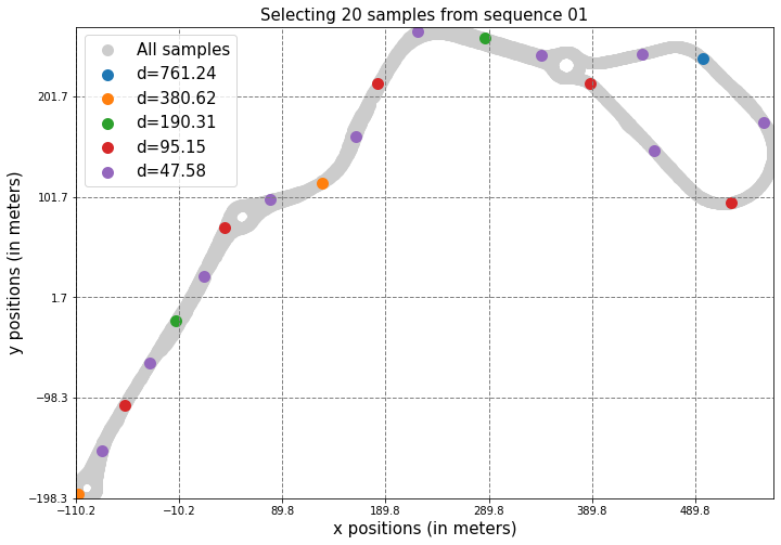
Figure 4: Selected poses using ego-pose distance based sampling on Navya3DSeg sequence 01 across various distance thresholds.

VI-B Active learning dataset distillation benchmark

To evaluate the performance of AL on Navya3DSeg, we use the standard mIoU metric for semantic segmentation, computed at the end of each AL step, on the entire label set, but also on things and stuff grouped labels. Besides, we measure the Labeling Efficiency (LE) [30] to compare the amount of data needed to achieve baseline performance for the different sampling techniques benchmarked, with respect to the random sampling technique.

The table VII presents the experiments settings. We use three different heuristics: Random Sampling (RS), our ego-pose Distance Sampling (DS) and BALD [31]. To speed up this process of heuristic computation, we can apply a random subset sampling over the unlabeled pool, termed as RSS. This reduces the number of model outputs being evaluated. In the same way, the ego-pose distance is used to select a subset from large unlabeled pool, and is termed as DSS. Once a prior subsampling is done on the unlabeled pool, we evaluate the heuristic function on selected subset. When using the BALD heuristic, we use the Inverse Label Frequency (ILF) to weight the heuristic score of each pixel. This reduces the impact of high frequency labels like ROAD or VEGETATION. Initial model of run (B) is the model trained on initial set sampled by run Random (A). Initial model of runs (D) and (E) is the model trained on initial set sampled by distance, which is run (C).

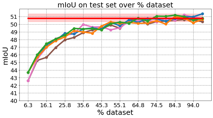
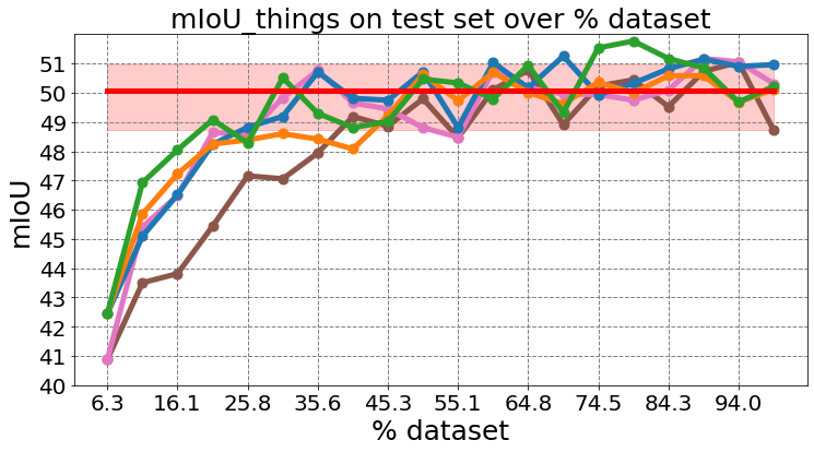
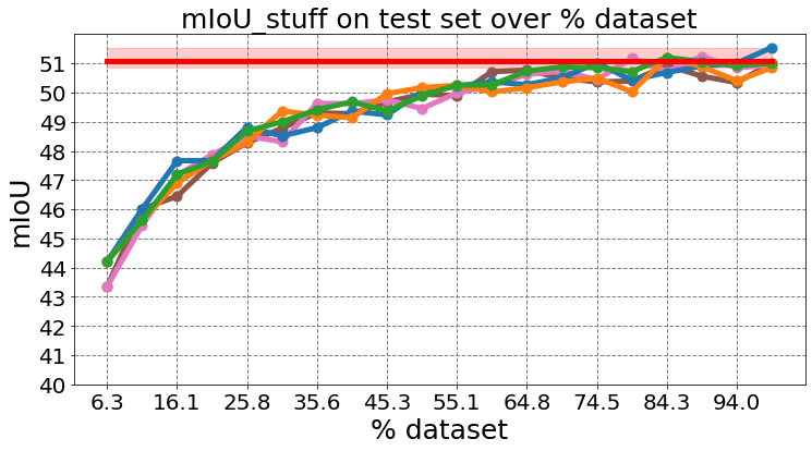
Figure 5: Navya3DSeg distillation results. Values on the legend are averages of LE ratios based on mIoU.

TABLE VII: Active learning benchmark

Run ID	Heuristic	Unlabeled pool Sub-sampler	Label Efficiency	Initial model
(A)	RS	-	1.0	run (A)
(B)	BALD	RSS	1.182
(C)	DS	-	1.261	run (C)
(D)	BALD	DSS	1.198
(E)	BALD+ILF	DSS	1.314

Experiment settings: Following our previous work [27], we use a Bayesian AL loop employing MC Dropout for uncertainty estimation. However, here we filter out pixels in range image which do not belong to any point in point clouds, then we use mean as an aggregation function to combine all pixel-wise scores of an image into a single score. The runs with subset sampling (B), (D) and (E), sample unlabeled pool into a subset with a size of 10000 samples before computing the uncertainty scores. For each AL step, all runs (tab. VII) are evaluated on a fixed test set from Navya3DSeg default split (section IV). The rest is used for the AL pool. We use SalsaNext as the semantic segmentation architecture, with parameters from table VIII.

TABLE VIII: Active learning experiments settings

Cyclic Learning rate		Early stopping
step size	policy	metric	patience	delta
6 epochs	triangular1.5	train loss	12 epochs	0.02
batch size			Initial pool	budget	AL step	aggregation
34	3055	2000	20	sum

Results and analysis: According to results in Fig. 5, all runs reach the lower bound of baseline performance with only 60% of data from the full dataset. Run (E) reaches the average of baseline performances with the lowest percentage of data from the full dataset, namely 64.8%, among all runs. At the first AL steps, all runs with subset samplings - (B), (D), (E) - and ego-pose Distance Sampling (C) outperform Random Sampling (A). In general, the method from run (E) outperforms the other ones, especially on things labels which represent only 5.06% of the whole labeled set. We can see that the stuff labels are more stable and have higher score than the things labels across the different AL steps. Subsequently, new extension of the dataset should considerably help to improve models’ performance on the things labels. Regarding model initialization, models trained on the initial pool generated by our proposed ego-pose distance based method have better results than random sampling.

VII Conclusion

We have presented Navya3DSeg, a highly diverse large scale semantic segmentation dataset on LiDAR point clouds for production grade autonomous driving applications. We have demonstrated sequential dataset splitting using multi-label stratified sampling techniques on both Navya3DSeg and SemanticKITTI datasets, and show consequent gains in performance generalization. A benchmark on key semantic segmentation models is provided, along with a study of dataset distillation using Bayesian Active Learning framework. Our novel ego-pose distance based sampling provides a fast and efficient way to distill the dataset to 64.8% to reach fully supervised performance on semantic segmentation task. Finally, we highlight that Navya3DSeg contains a large unlabeled pool of scans from varied operational domains of the autonomous shuttle to evaluate self-supervised and semi-supervised methods for future work.

Navya3DSeg - Navya 3D Semantic Segmentation
Dataset Design & split generation for autonomous vehicles
- Supplementary Materials -

Figure 6: Navya3DSeg complex curbs examples, with the curb label highlighted in yellow.

VIII Navya3DSeg dataset

The Navya3DSeg dataset provides production grade labeled point clouds for the task of semantic segmentation. The semantic descriptions of the different labels in the dataset are key to understand the features and objects that are annotated. The Navya3DSeg labels’ definitions, provided in Tab.XIII, were used to define the dataset’s annotation policy.

Navya3DSeg dataset introduces the CURB label which is missing in most large scale semantic segmentation datasets. Bai et al. [16] highlight the lack of a dedicated CURB label in point cloud datasets, and discuss classical processing methods to extract them at a large scale. The CURB label represents 1.379% of Navya3DSeg, namely 21,45 million points coming from various environments, from national road to urban areas, including some complex cases like crossroad and driveways which are useful for HDMap and road map generation. Fig. 6 shows Navya3DSeg sequences with a highlight on the CURB label.

IX Dataset split generation

IX-A Stratified Sampling for Sequences

In standard MSSS implementation (Algo.1), Sechidis et al. [18] iteratively assign samples based on label frequency to the different k-splits, going from least to most frequent in the remaining samples. Given the subset index j and the class index i, MSSS starts by calculating the remaining desired number of samples $c_{j}$ and desired number of samples per label $c^{i}_{j}$ for each subset (train, val, test). In each iteration, the algorithm examines label $l$ having the fewest number of remaining samples (line 1) and stratifies its samples into output subsets $S_{m}$. The output subset $S_{m}$ for each sample is selected based on the most desired number of samples $c^{i}_{j}$ (line. 1) then $c_{j}$ (line. 1).

Due to the effect of aggregation of samples into larger segments, several labels land-up with similar frequencies with standard MSSS implementation which considers only the binary presence/absence of label in large segment. For example, in case of a split by sequence, the number of occurrences of a label in every sequence is the number of sequences containing that label, which might end up to be the same for several labels. In this case (line. 1), we choose the label having a distribution across all samples furthest away from the uniform distribution instead of the number of presences/absences of label in all segments.

Input : A set of instances, D, annotated with a set of labels $L={\lambda_{1},...,\lambda_{q}}$, desired number of subsets k, desired proportion of samples in each subset $r_{1},...r_{k}$

Output : Disjoint subsets $S_{1},...S_{k}$ of D

/* Calculate the desired number of samples at each subset */

for $j\leftarrow 1$ to $k$ do

       $c_{j}=|D|r_{j}$

      

end for

/* Calculate the desired number of samples of each label at each subset */

for $i\leftarrow 1$ to $L$ do

       for $j\leftarrow 1$ to $k$ do

             $c^{i}_{j}\leftarrow|D^{i}|r_{j}$

            

       end for

      

end for

while $|D|>0$ do

       /* Find the label with the fewest (but at least one) remaining samples */

       $l\leftarrow\textbf{argmin}_{i}(|D^{i}|)$

      foreach $(x,Y)\in D^{L}$ do

             /* Find the subset(s) with the largest number of desired samples for this label */

             $M\leftarrow\textbf{argmax}_{j=1...k}(c^{l}_{j})$

             if $|M|=1$ then

                   $m\in M$

                  

             else

                   /* Prioritize the subset(s) with the largest number of desired samples */

                   $M^{\prime}\leftarrow\textbf{argmax}_{j\in M}(c_{j})$

                   if $|M^{\prime}|=1$ then

                         $m\in M^{\prime}$

                        

                   else

                        

                        $m\leftarrow\textit{randomElementOf}(M^{\prime})$

                        

                   end if

                  

             end if

            

            $S_{m}\leftarrow S_{m}\bigcup(x,Y)$

             $D\leftarrow D\backslash\{(x,Y)\}$

            

            /* Update desired number of samples */

             foreach $\lambda_{i}\in Y$ do

                   $c^{i}_{m}\leftarrow c^{i}_{m}-1$

                  

             end foreach

            $c_{m}\leftarrow c_{m}-1$

            

       end foreach

      

end while

Algorithm 1 IterativeStratification $(D,n,r_{1}...r_{n})$

IX-B Navya3DSeg split

Following our strategy for dataset split choice, the Navya3DSeg split (Fig. 7) is the one that satisfies the most of our multiple objectives. With a desired ratio of 0.7:0.1:0.2 for train:validation:test subsets and a sequence level granularity, we selected the sequences 12, 15, 18, 19 and 22 as our test set. The actual ratio of train:validation is 79.8:20.2 despite the 87.5:12.5 desired ratio. This shift is the consequence of the sequence level granularity, which was mandatory to preserve a consistent test set, which labels will remain hidden. The figure 7, namely label representation, shows the ratio of each label in the train and validation subsets over the full Navya3DSeg.

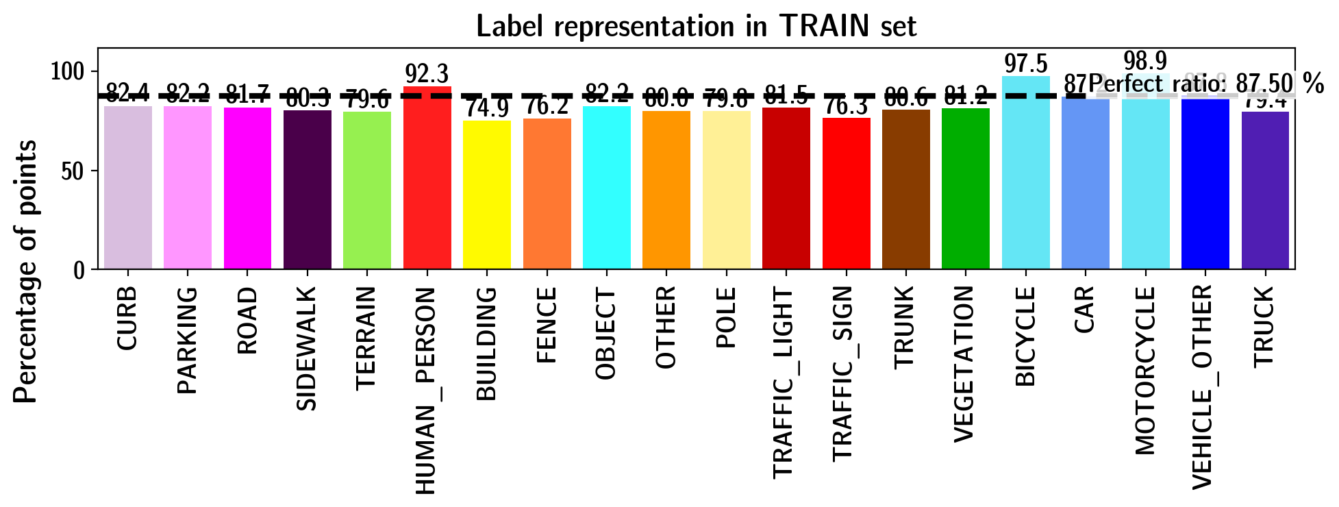
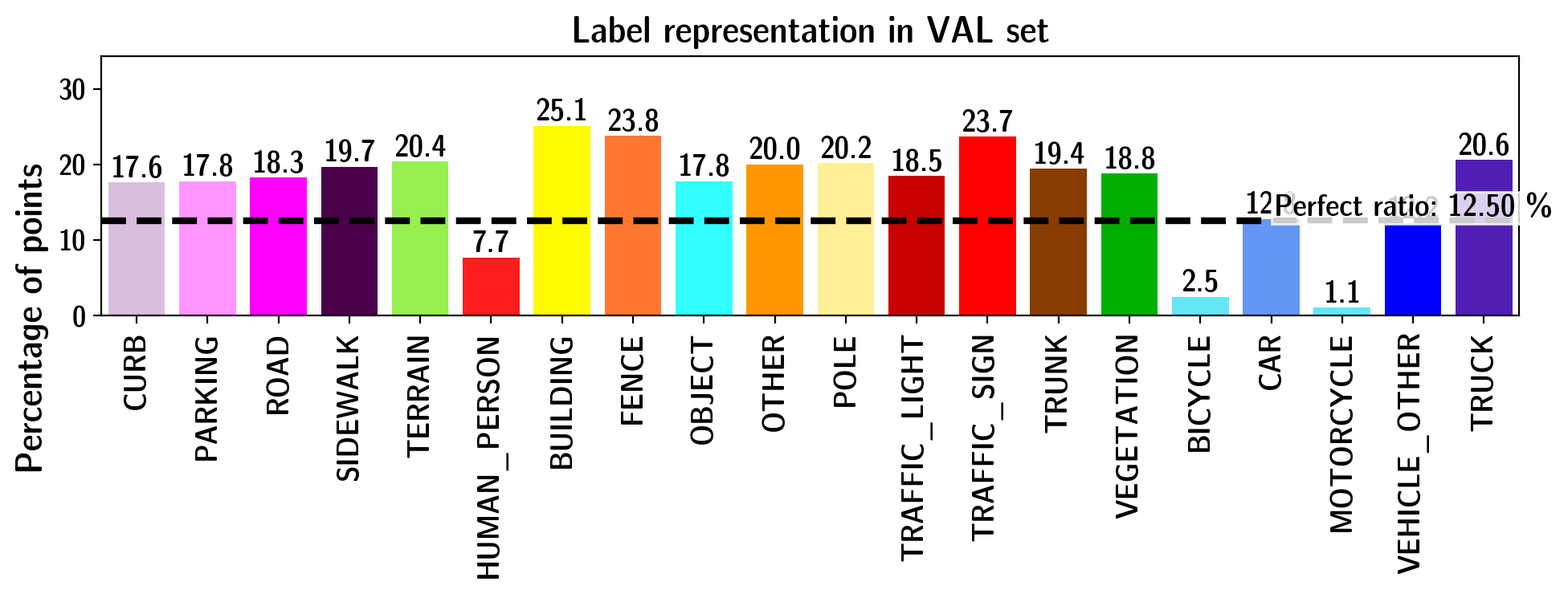
Figure 7: Label representation of Navya3DSeg selected split with a desired ratio of 87.5:12.5 for train:validation subsets.

The figure 8 shows the intensity distribution of each subset and the IDS corresponding to the splits of both Navya3DSeg and SemanticKITTI. These two datasets were built with different LiDAR sensors, from two different manufacturers. It explains the different shapes of the intensity distributions between the two datasets. Compared to SemanticKITTI, the selected split of Navya3DSeg is less prone to intensity distribution shift.

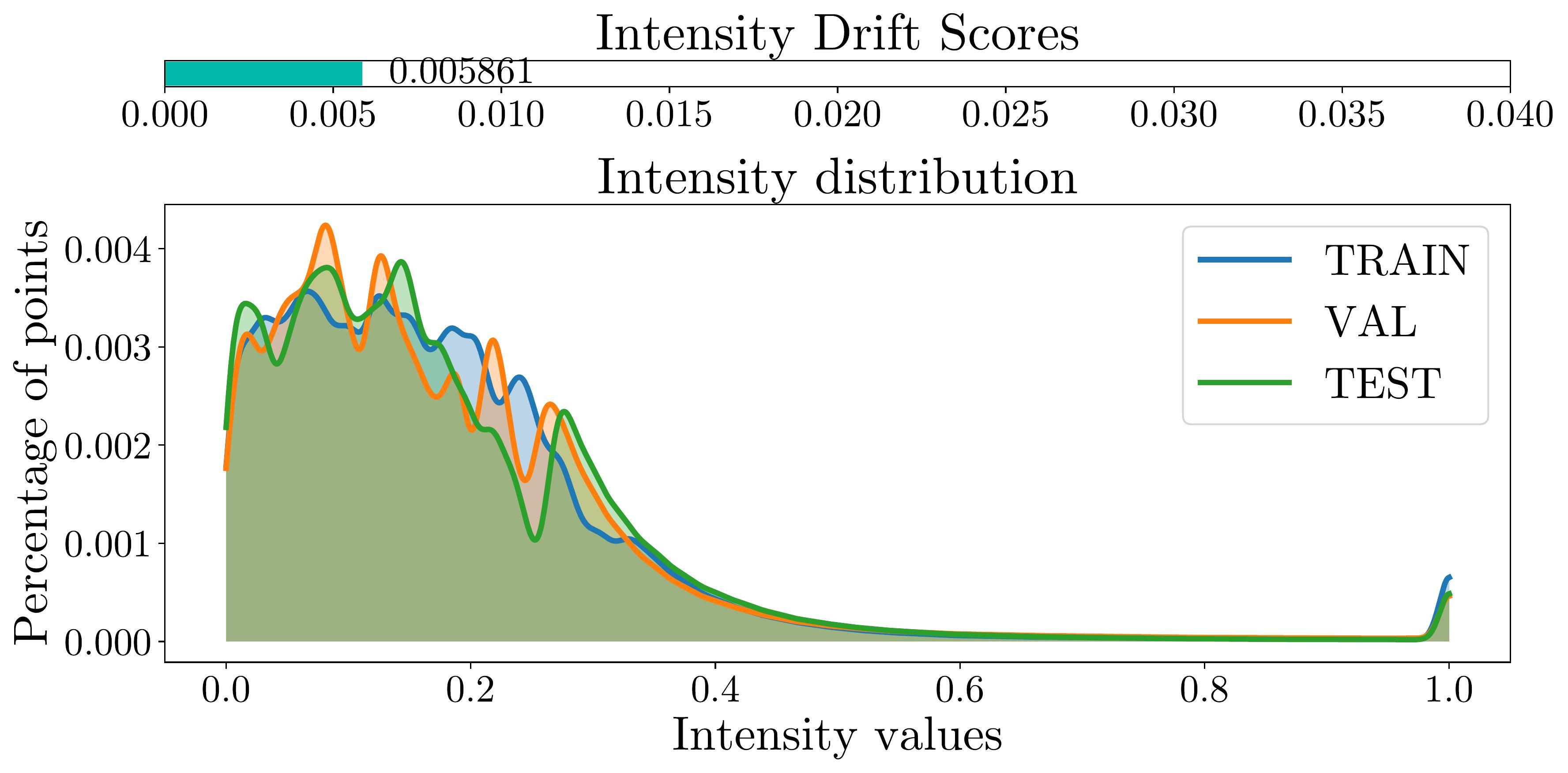
(a) Navya3DSeg

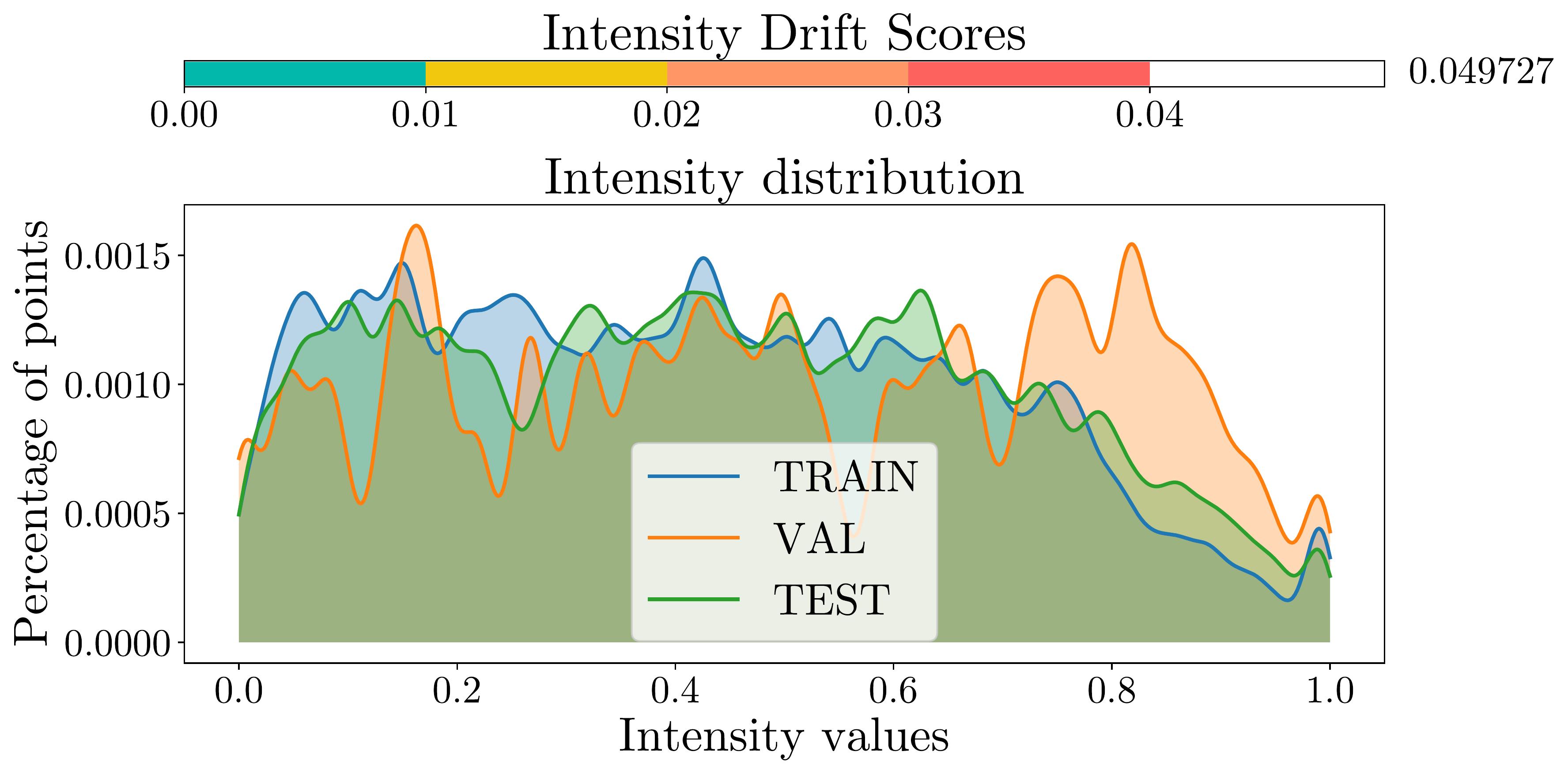
(b) SemanticKITTI

Figure 8: Intensity distribution drift.

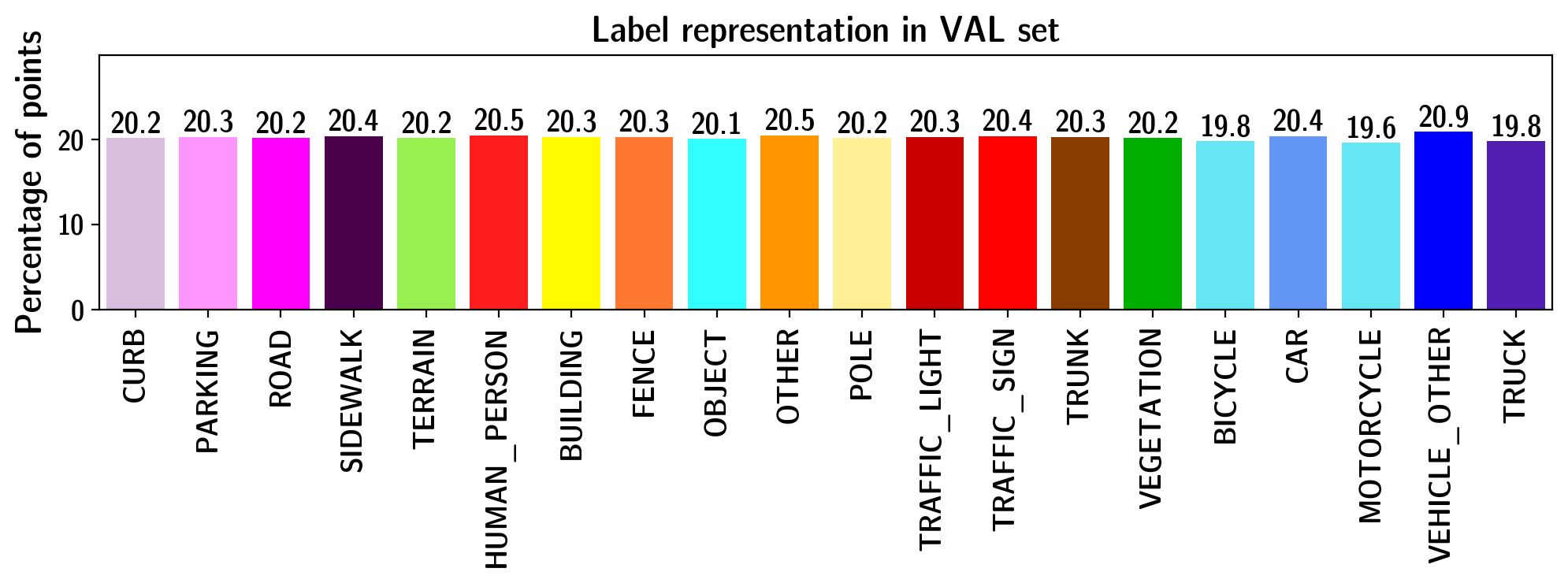
(a)

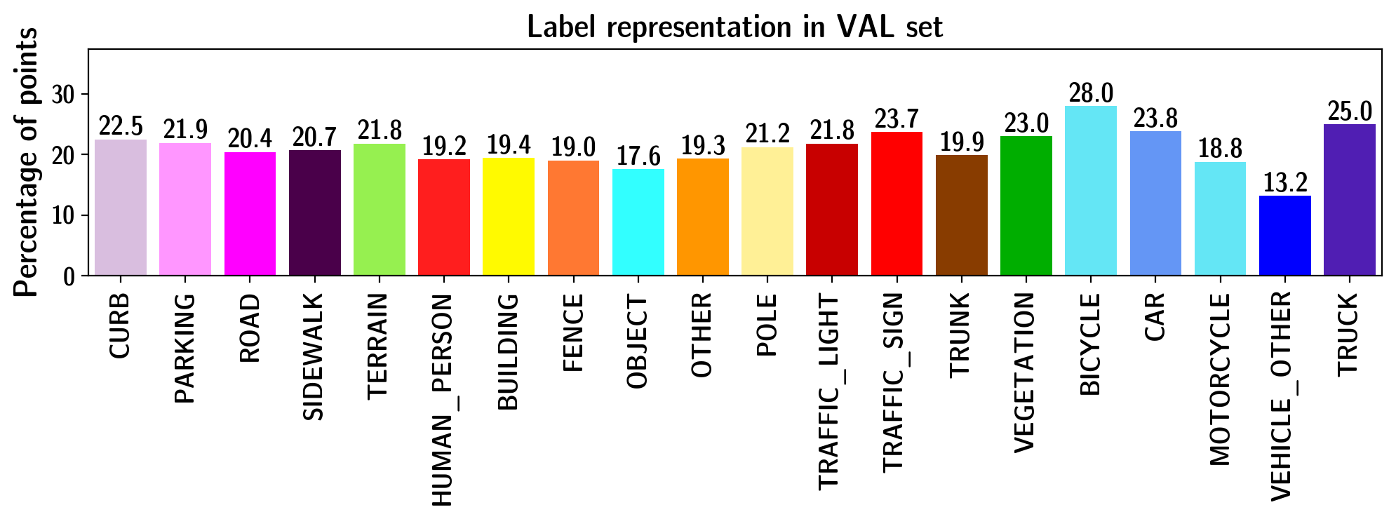
(b)

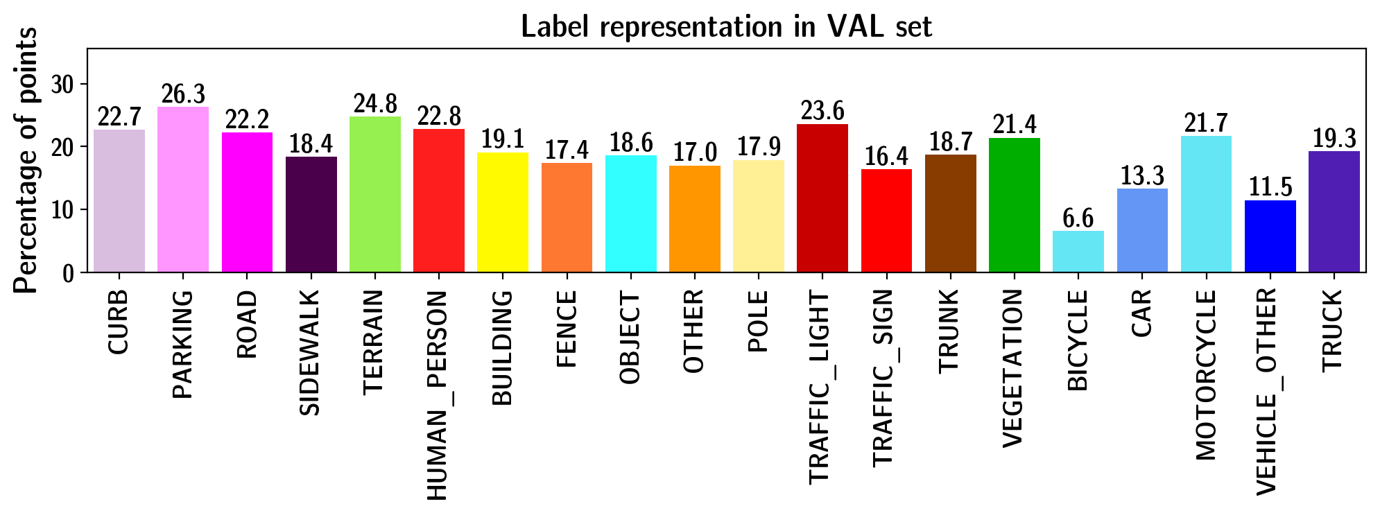
(c)

Figure 9: Label representation of validation sets split by granularity of 1 (a), 500 (b) and 2000 (c) on Navya3DSeg

IX-C Granularity experiments

Datasets containing sequential information such as point clouds sequences like in Navya3DSeg, or object tracking data in images could use the granularity parameter to define the level of aggregation to group individual samples. It allows advanced configuration to perform stratified sampling, with the Multi-label Stratified Shuffle Split (MSSS) technique, or our Multi-label Segment Stratified Shuffle Split (MSegSSS) technique. A reminder of our granularity benchmark is available at Tab. IX. The label distributions among subsets are presented in Fig. 9 for Navya3DSeg, and in Fig. 10 for SemanticKITTI.

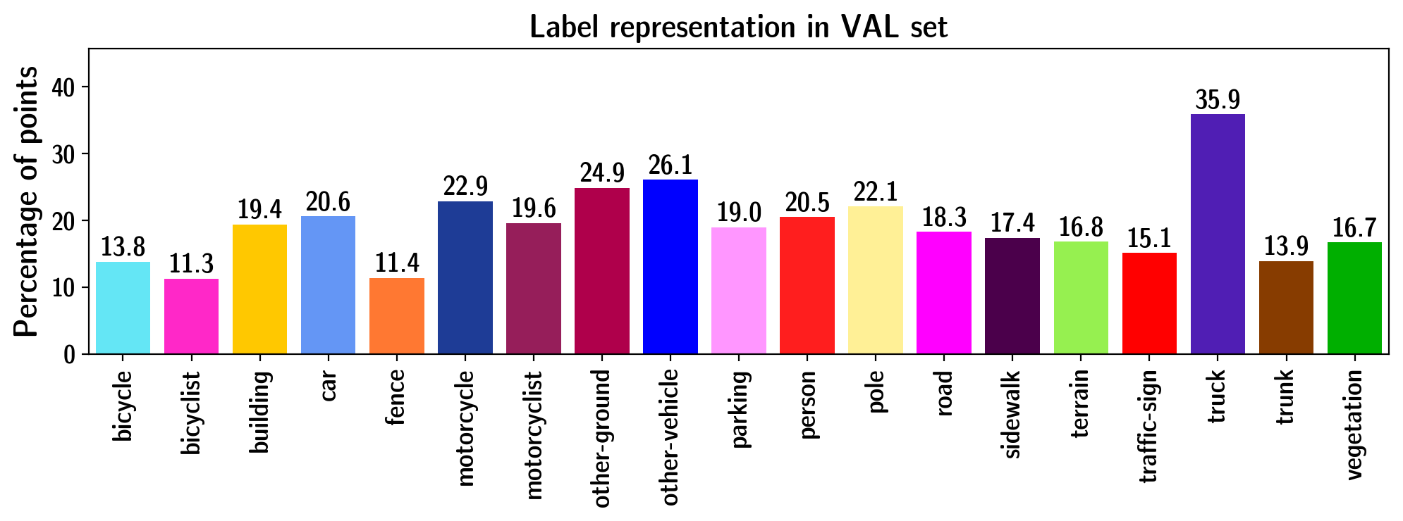
(a)

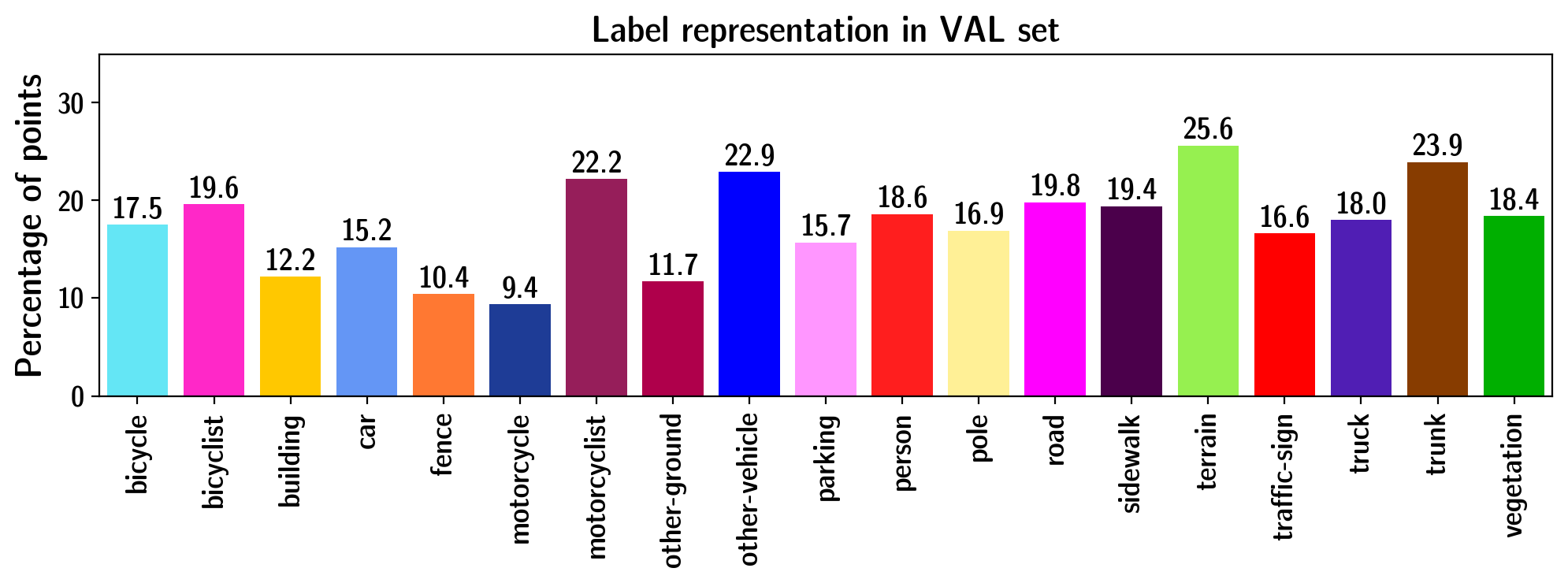
(b)

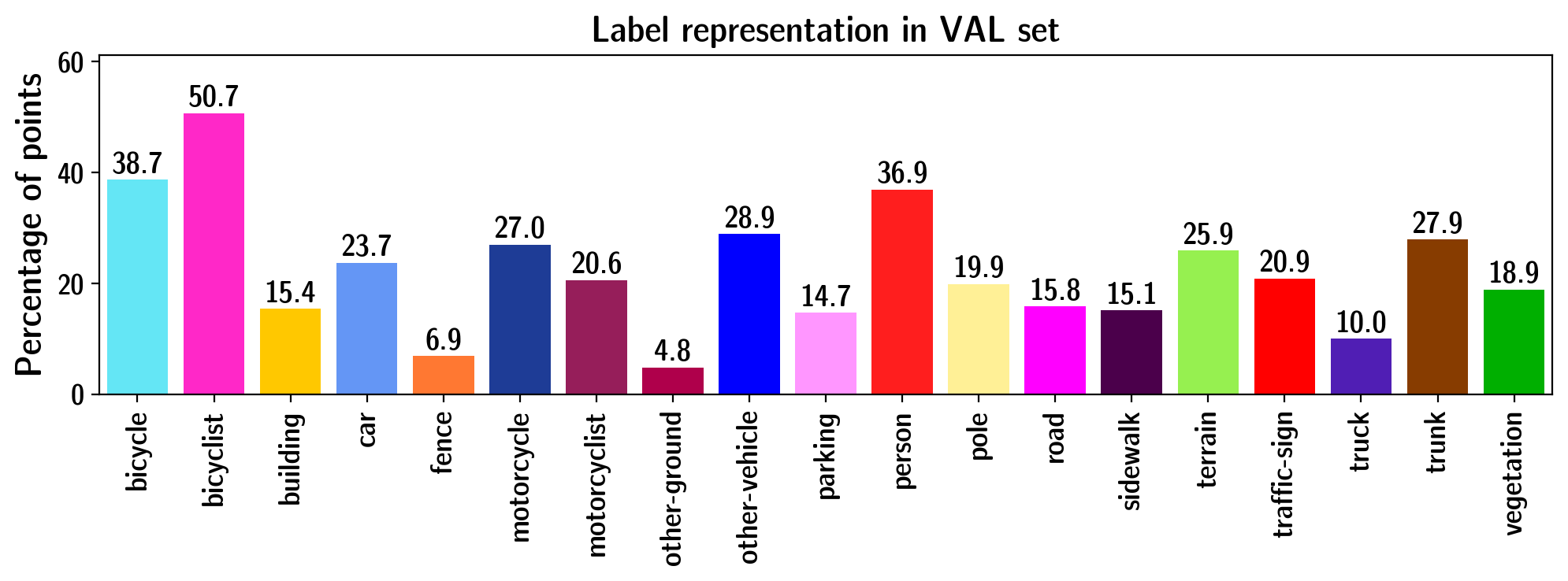
(c)

Figure 10: Label representation of validation sets split by granularity of 500 (a) and 1000 (b) on SemanticKITTI and default validation set composed of sequence 08 (c). Dynamic labels are fused with static labels.

TABLE IX: Granularity evaluation on Navya3DSeg and SemanticKITTI. The sequence split (Sequence*) of SemanticKITTI was taken from the dataset configuration

Dataset	Input variables		Output metrics
	Granularity	Targeted ratios	Obtained ratios	LD $\downarrow$	IDS $\downarrow$	KL Divergence $\downarrow$	Train mIoU	Val mIoU	Test mIoU
Navya3DSeg	Sequence	87.5:12.5	79.8:20.2	5,10E-03	5,90E-03	6,45E-03	73.15	45.67	50.69
	2000	87.5:12.5	87.3:12.7	4,60E-03	1,80E-02	7,01E-03	69.03	47.27	48.30
	$2000^{\dagger}$	79.8:20.2	79.5:20.5	4,30E-03	6,00E-03	4,27E-03	72.05	47.93	49.37
	500	79.8:20.2	79.0:21.0	4,70E-03	3,60E-03	1,62E-03	72.77	54.59	50.49
	1	79.8:20.2	79.7:20.3	2,00E-04	1,00E-04	7,00E-06	72.10	72.72	51.09
SemanticKITTI	Sequence*	-	82.7:17.3	8,10E-03	6,53E-02	1,87E-02	80.84	53.66	54.81
	1000	82.7:17.3	82.0:18.0	6,80E-03	3,50E-03	1,31E-02	81.62	61.43	56.00
	500	82.7:17.3	82.5:17.5	3,40E-03	2,70E-03	4,35E-03	82.47	64.03	55.97

X Semantic segmentation benchmark

X-A Hyper-parameters & Training setup

The table X shows the hyper-parameters and training set up for all experiments on Navya3DSeg, including dataset splitting, semantic segmentation benchmark, cross-dataset generalization, and dataset distillation with active learning. For the cyclic learning rate, we apply the implementation from PyTorch [32]. To perform an efficient benchmark, and lower the effect of label imbalance, we perform a label mapping, described in Tab. XIV, to gather some labels.

TABLE X: Models’ hyper-parameters of training used in our different experiments. The triangular1.5 and triangular1.25 policies are similar to the standard triangular policy, but instead it cuts our max learning rate bound in 1.5 and 1.25 respectively, after every cycle

Model	weight decay	Momentum	Batch size	Epochs
SalsaNext	0,0001	0,9	36	150
&	Cyclic Learning rate (LR) scheduler[32] [33]
SqueezeSegV2	Policy	Max LR	Base LR	Step size
	Triangular 1,25	0,1	0,001	8 epochs
Cylinder3D	weight decay	Momentum	Batch size	Epochs
	0,0001	0.9	10	150
	Cyclic Learning rate (LR) scheduler[32] [33]
	Policy	Max LR	Base LR	Step size
	Triangular 1,25	0,001	0,00001	8 epochs

X-B Benchmark results

The results from our semantic segmentation benchmark are presented in Tab. XII. Overall, Cylinder3D performs better than the range image based architectures SqueezeSegV2 and SalsaNext. We plot the performance of these three baseline models over different ranges of operation in Fig. 11.

X-C Cross-dataset generalization between Navya3DSeg and SemanticKITTI

We extracted a common label space (Tab. XV) containing only labels available in both datasets’ validation set and showing consistent annotation policies. For this experiment we performed the source-target label map dynamically. Because of SemanticKITTI’s size and point cloud density, we expected to have better results when training on SemanticKITTI and evaluating on Navya3DSeg. However, Tab. XI shows that models trained on Navya3DSeg perform better on things labels and on most of the ground labels, except GROUND_ROAD, and MANMANDE_BUILDING which are in the top-3 most represented class in SemanticKITTI, explaining the mIoU_Stuff score drop during evaluation. This can be explained by: 1. the Navya3DSeg sensor orientation which enhance the ground focus, and 2. by the spherical representation with this orientation, which distorts the projected range-image. Thus, when performing evaluation from Navya3DSeg, labeled points from the front and the rear of the mapping vehicle are highly impacted, contrary to the labeled points on the sides of the mapping vehicle. These differences in label distribution are highlighted in Fig. 14 and Fig. 15.

TABLE XI: Cross dataset generalization results between SemanticKITTI and Navya3DSeg on validation set with SalsaNext architecture

Train dataset	Validation dataset	mIoU Things	mIoU Stuff	Road	Building	Terrain	Vegetation	Trunk	Car	Traffic Sign
SemanticKITTI	Navya3DSeg	12.94	22.82	46.72	55.85	10.66	40.39	4.68	21.42	11.81
Navya3DSeg	SemanticKITTI	17.55	16.36	13.89	17.71	14.17	52.45	14.67	29.40	22.14

TABLE XII: Semantic segmentation benchmark on Navya3DSeg test and validations sets

Subset	Model	Things labels		Stuff labels		mIoU	fwIoU
		mIoU	fwIoU	mIoU	fwIoU
Validation	SalsaNext	43,73	1,41	46,50	69,48	45,67	70,88
	SqueezeSegV2	27,87	1,22	35,10	59,67	32,93	60,89
	Cylinder3D	58.69	1.72	54.23	75.85	55.57	77.57
Test	SalsaNext	50,18	2,25	50,90	71,86	50,69	74,11
	SqueezeSegV2	37,71	1,93	40,12	65,59	39,39	67,52
	Cylinder3D	68.40	2.66	60.46	78.50	62.84	81.16

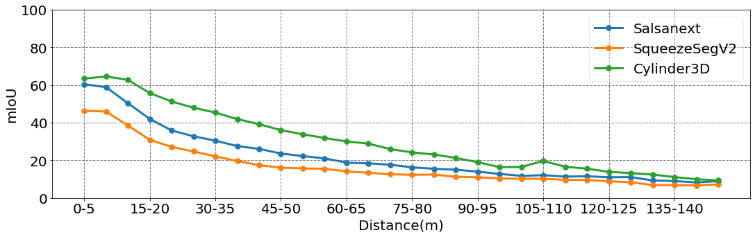
(a)

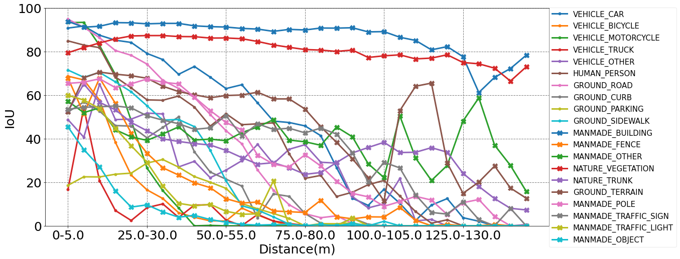
(b)

Figure 11: (a): mIoU vs Distance plots for our trained models from 3 different architectures. (b): Label IoU plots for the Cylinder3D model.

XI Dataset distillation with Active Learning

XI-A ego-pose distance based sampling

Ego-pose distance based sampling (detailed in Algo. 2) can be adapted either offline or online in an active learning setup. In terms of practical implementation, we use the BallTree from sklearn.neighbors to naively find neighbors within a radius, and euclidean distance as the distance between two point clouds.

Input : labeled pool $L$, unlabeled pool $U$, budget $b$

/* Compute the maximum distance between labeled and unlabeled samples’ ego-poses */

if $L=\emptyset$ then

      $d=$MaxDistance(U, U)

else

      $d=$MaxDistance(L, U)

end if

/* Find unlabeled samples the don’t belong to the neighbors of L within a radius d */

$A=\{x|x\in U,\forall y\in L,\text{dist}(x,y)>d\}$

$S=\emptyset$

for $n\leftarrow 1$ to $b$ do

       while $A=\emptyset$ do

             d = reduce(d) /* reduce radius d */

             /* Find unlabeled samples that don’t belong to the neighbors of L and S within a radius d */

             $A=\{x|x\in U\setminus S,\forall y\in L\sqcup S,\text{dist}(x,y)>d\}$

       end while

      

      if $S\neq\emptyset$ then

            

            /* select a sample in A having the maximum distance to its closest point in S. */

             $s\leftarrow\{x|\text{dist}(x,y)=\max_{x^{\prime}}\text{dist}(x^{\prime},y),~{}\text{dist}(x^{\prime},y)=\min_{y^{\prime}}dist(x^{\prime},y^{\prime}),\forall x^{\prime}\in A,\forall y^{\prime}\in S\}$

       else if $L\neq\emptyset$ then

             /* select a sample in A having the maximum distance to its closest point in L. */

             $s\leftarrow\{x|\text{dist}(x,y)=\max_{x^{\prime}}\text{dist}(x^{\prime},y),~{}\text{dist}(x^{\prime},y)=\min_{y^{\prime}}dist(x^{\prime},y^{\prime}),\forall x^{\prime}\in A,\forall y^{\prime}\in L\}$

       else

             $s\leftarrow$ randomly select a sample in A.

       end if

      

      $S\leftarrow S\cup\{s\}$

end for

Output : selected samples $S=\{s_{1},...,s_{b}\}$

Algorithm 2 Ego-pose distance based sampling proposed method

XI-B Active learning benchmark

Metrics Given a specific value of mIoU, the Labeling Efficiency (LE) based on mIoU is the ratio between the number of labeled range images, acquired by the baseline sampling and the other sampling techniques.

$$\text{LE}=\frac{n_{\text{labeled}\_\text{others}}(\text{mIoU}=a)}{n_{\text{labeled}\_\text{baseline}}(\text{mIoU}=a)}$$ (3)

The baseline method in our experiment is the random heuristic.

Extra results According to Fig. 12, our ego-pose distance based sampling method gives the best performance on stuff labels, whereas BALD and Inverse Label Frequency (IFL) focuses on things labels. Among things labels (Fig. 16), VEHICLE_CAR and VEHICLE_OTHER have the most visible performance improvement between Random (RS) and the other methods. On the contrary, stuff labels (Fig. 17) are more stable for all methods, but their performances still increase as AL steps increase. Fig. 13 shows the top 3 hardest and easiest selected samples of our best strategy (DSS+BALD+ILF).

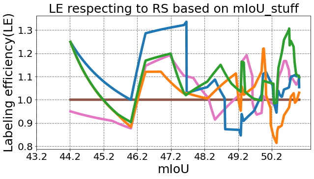
(a)

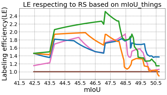
(b)

Figure 12: Navya3DSeg dataset distillation results. Values on the legend are the averages of LE ratios based on stuff mIoU (b) and things mIoU (c).

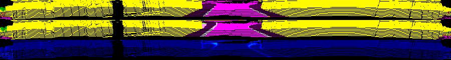
(a) sequence 08 scan 000305

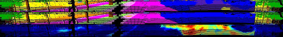
(b) sequence 14 scan 001508

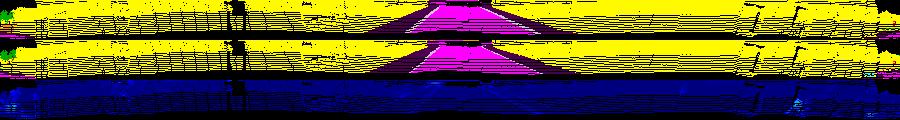
(c) sequence 08 scan 000299

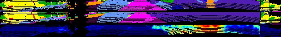
(d) sequence 06 scan 003453

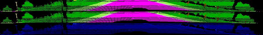
(e) sequence 02 scan 002503

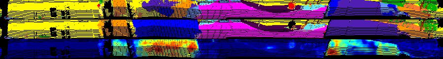
(f) sequence 14 scan 002710

Figure 13: Active learning sample selection examples for DSS+BALD+ILF run. For each scan, from top to bottom, images are prediction, ground truth and BALD score. (a), (c) and (e): Top 3 easiest samples in subset. (b), (d) and (e): Top 3 hardest samples in subset.

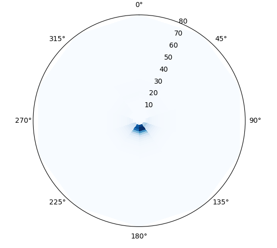
(a) Navya3DSeg ROAD

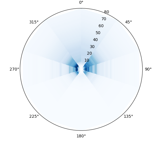
(b) Navya3DSeg BUILDING

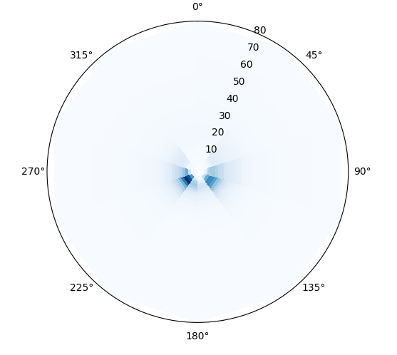
(c) Navya3DSeg TERRAIN

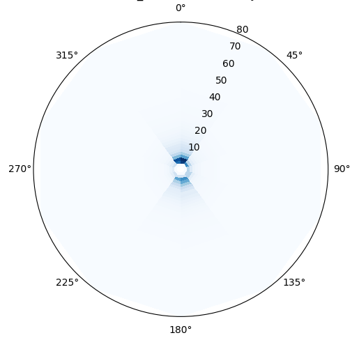
(d) SemanticKITTI ROAD

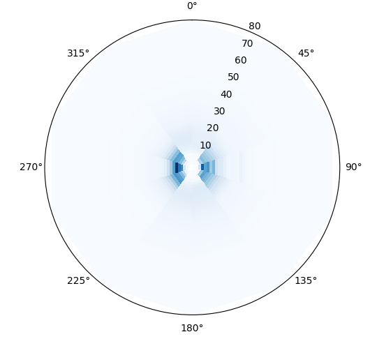
(e) SemanticKITTI BUILDING

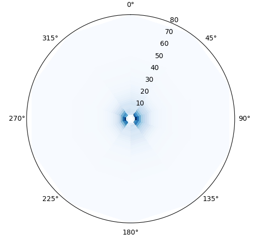
(f) SemanticKITTI TERRAIN

(g) Navya3DSeg TERRAIN

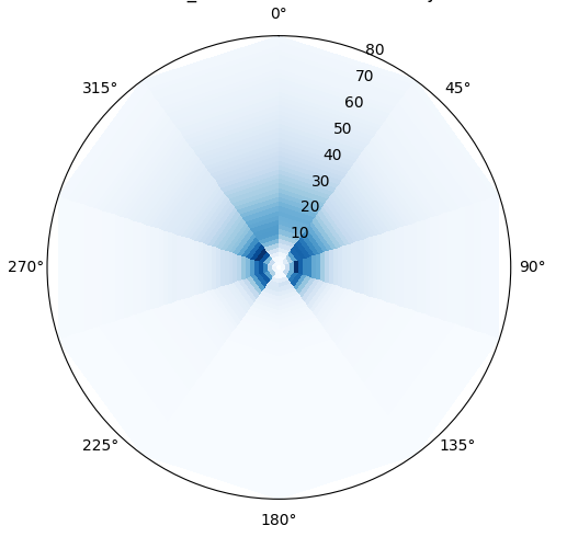
(h) Navya3DSeg VEGETATION

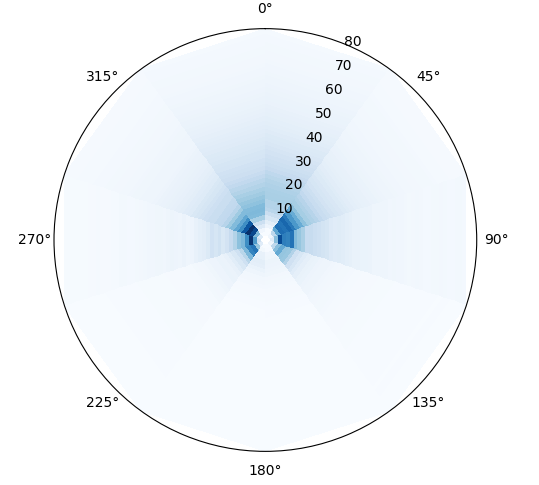
(i) Navya3DSeg TRUNK

(j) SemanticKITTI TERRAIN

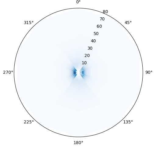
(k) SemanticKITTI VEGETATION

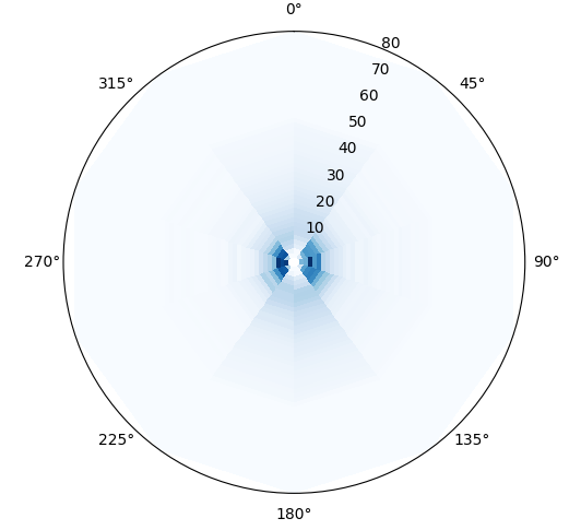
(l) SemanticKITTI TRUNK

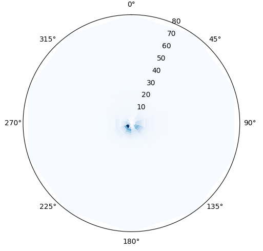
(m) Navya3DSeg CAR

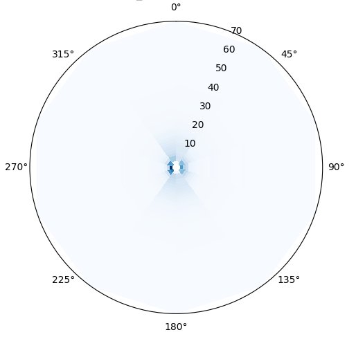
(n) SemanticKITTI CAR

Figure 14: Polar density plot of highlighted labels for cross dataset generalisation experiment between Navya3DSeg and SemanticKITTI. The maximum radius has been set following SemanticKITTI annotation distance. Those plots emphasize the impact of Navya3DSeg sensor orientation compare to a flat configuration in SemanticKITTI.

(a) Navya3DSeg ROAD

(b) SemanticKITTI ROAD

(c) Navya3DSeg BUILDING

(d) SemanticKITTI BUILDING

(e) Navya3DSeg TERRAIN

(f) SemanticKITTI TERRAIN

(g) Navya3DSeg VEGETATION

(h) SemanticKITTI VEGETATION

(i) Navya3DSeg TRUNK

(j) SemanticKITTI TRUNK

(k) Navya3DSeg CAR

(l) SemanticKITTI CAR

Figure 15: Density range-images of highlighted labels for cross dataset generalisation experiment between Navya3DSeg and SemanticKITTI. No point limit has been set for spherical projection. Those plots shows the impact of spherical projection based on inclined sensor data.

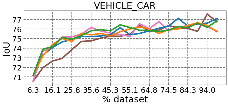
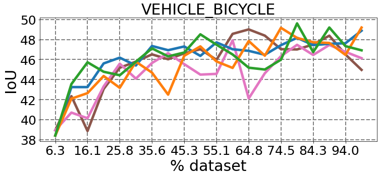
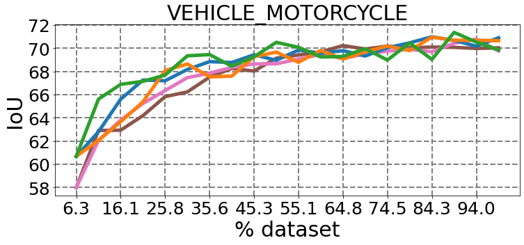
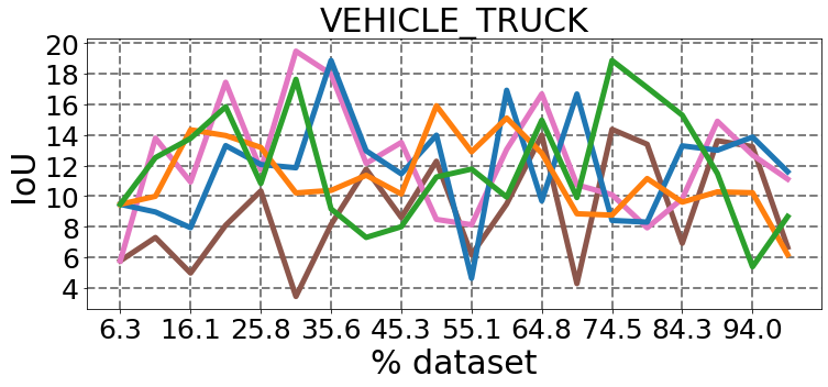
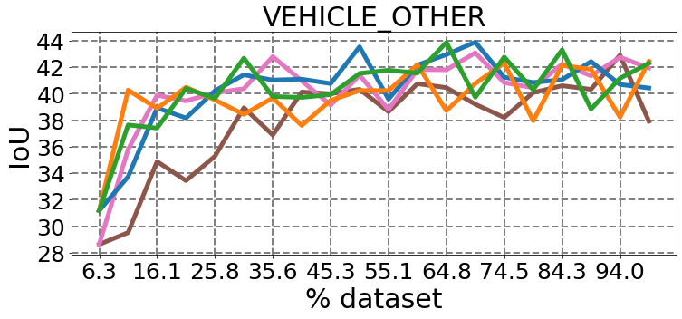
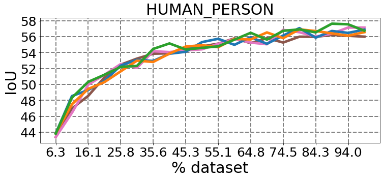
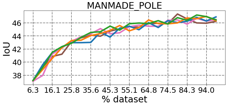
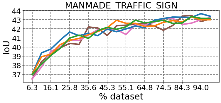
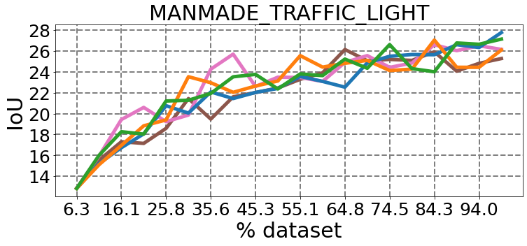
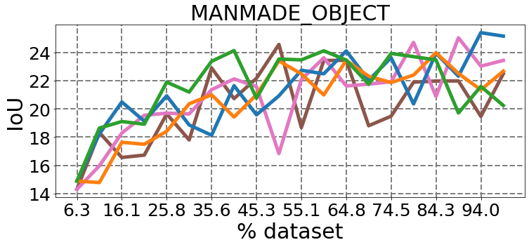
Figure 16: IoU vs % dataset of things labels.

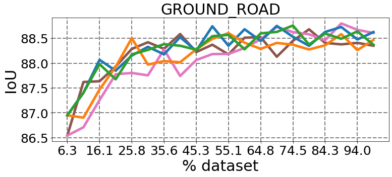
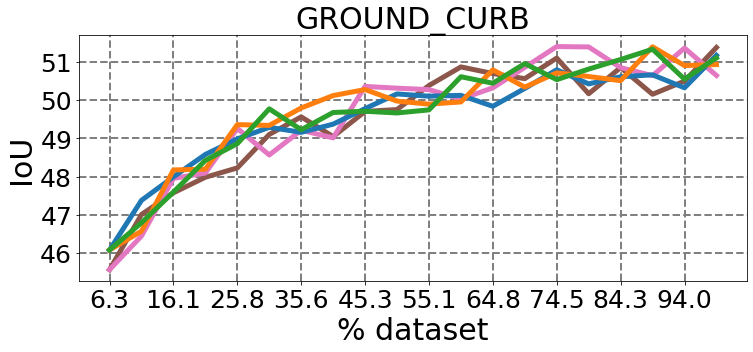
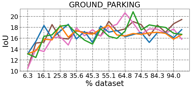
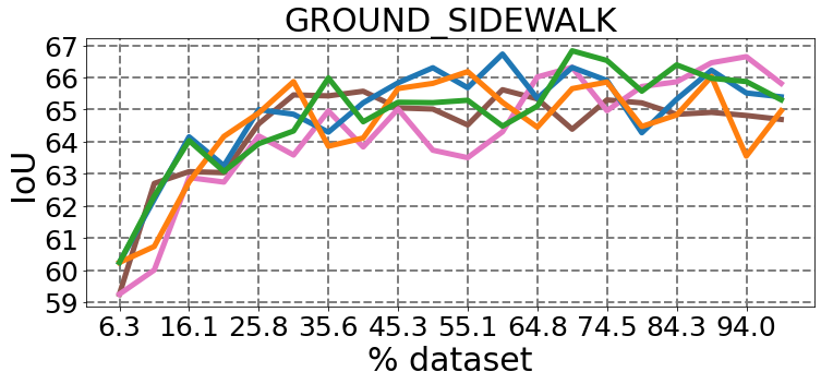
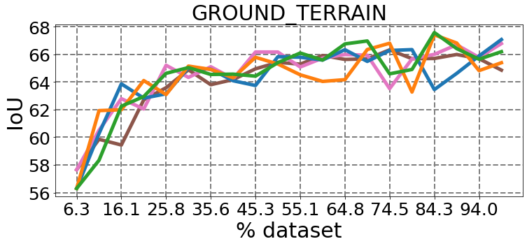
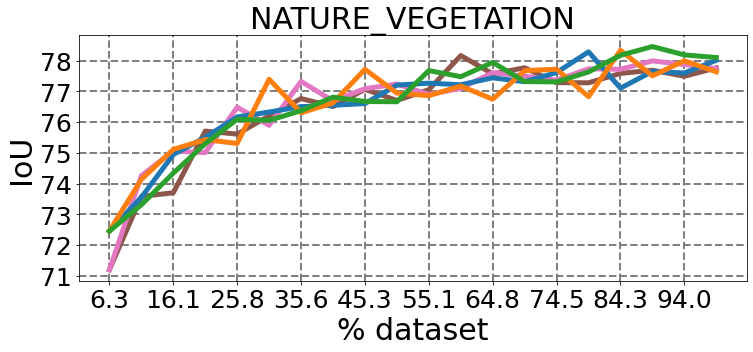
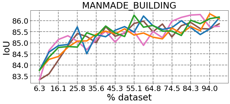
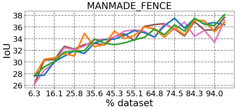
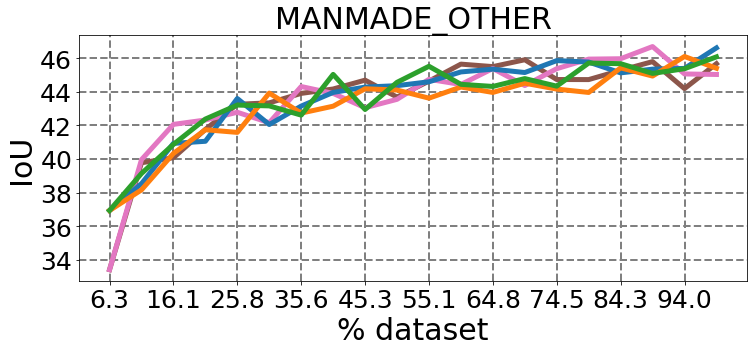
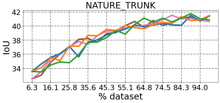
Figure 17: IoU vs % dataset of stuff labels.

TABLE XIII: Navya3DSeg labels definition

Category	Label	Definition
Other	UNKNOWN	Undefined object or stuff
	OTHER	Outlier points, caused by reflections or from mapping vehicle track for example
Vehicle	CAR	4-wheels cars, sedan, SUV, city car, vans with a continuous cabin
	BICYCLE	2-wheels bicycle without the rider
	MOTORCYCLE	2-wheels motorcycle without the rider
	TRUCK	Trucks, vans with a body that is separated from the driver cabin, pickup trucks, with attached trailers.
	OTHER	Any vehicle that does not fit into the other category’s labels. Eg. bus, airplane, boat, another autonomous vehicle
Human	PERSON	Humans as pedestrians or riders of a vehicle
Ground	ROAD	Areas where motorized vehicles are supposed to move on
	SPEED_BUMP	Areas on the road materializing a speed bump, or only a slope intended to make a slow down
	PARKING	Areas where vehicles, such as cars, bicycles, motorcycles and trucks are allowed to park. An area where a car is parked is not considered as parking by itself (it can be an illegal parking)
	BICYCLE_LANE	Areas dedicated to bicycles only. Must be delimited at least by a lane marking
	CURB	Structures that delimits the slope between the road and the sidewalk
	PEDESTRIAN_CROSSING	Areas where the road marking is a zebra one, materializing a pedestrian crossing
	ZEBRA_ROAD_MARKING	Areas with painted road markings, showing a clear “no go zone” for any vehicle
	SIDEWALK	Areas dedicated to pedestrians only or areas dedicated to pedestrians and bicycles only.
	TERRAIN	Areas with grass and all other types of horizontal spreading vegetation, including soil, where a human can normally walk on. Any high vegetation (height >$\sim$20cm) must be considered as vegetation
	OTHER	Any kind of ground plane area that does not fit into the definitions of other ground labels
Manmade	BUILDING	Structures where a human can go inside. It can be a house, an office building, a skyscraper, a garage, a garden shed, …
	FENCE	Structures on the yz-plane, which contains holes in it. Flat and solid yz-areas should be considered as walls, which can belong to a building or manmade_other label.
	OTHER	Any kind of structure that does not fit into any other Manmade labels. It includes fixed structures where a human cannot go inside, art sculptures, toll gate, …
	POLE	Structures that can be considered as long, straight and vertical. It can be street lamp, electric pole, bollard or the structure meant to support traffic lights and signs. It also includes the structure at the top of the pole, like the street lamp itself.
	TRAFFIC_SIGN	Flat panels with traffic information written on it. Most of the time the surface is reflective. It can also be directions panels.
	TRAFFIC_LIGHT	Infrastructures to signal traffic with lights. Either 3-row traffic lights, or a single light.
	OBJECT	Objects that can be moved by a single human. Eg. traffic cone, trash can, flower pot, a bag, etc
Nature	VEGETATION	Vegetation where a human cannot normally walk on, including bushes, foliage
	TRUNK	Natural tree trunks, separated from the tree foliage
Dynamic	CAR	Dynamic tracks of vehicles belonging to the car label
	BICYCLIST	Dynamic tracks of bicycle or motorcycle
	PERSON	Dynamic tracks of human label
	TRUCK	Dynamic tracks of truck label
	OTHER_VEHICLE	Dynamic tracks of other_vehicle label

TABLE XIV: Benchmark label mapping from original Navya3DSeg to Navya3DSeg Benchmark with sub category information

Navya3DSeg Label	Benchmark Label	SubSet
UNKNOWN	UNKNOWN	None
OTHER	UNKNOWN	None
VEHICLE_CAR	VEHICLE_CAR	Thing
VEHICLE_BICYCLE	VEHICLE_BICYCLE	Thing
VEHICLE_MOTORCYCLE	VEHICLE_MOTORCYCLE	Thing
VEHICLE_TRUCK	VEHICLE_TRUCK	Thing
VEHICLE_OTHER	VEHICLE_OTHER	Thing
HUMAN_PERSON	HUMAN_PERSON	Thing
GROUND_ROAD	GROUND_ROAD	Stuff
GROUND_SPEED_BUMP	GROUND_ROAD	Stuff
GROUND_CURB	GROUND_CURB	Stuff
GROUND_PARKING	GROUND_PARKING	Stuff
GROUND_BICYCLE_LANE	GROUND_ROAD	Stuff
GROUND_PEDESTRIAN_CROSSING	GROUND_ROAD	Stuff
GROUND_ZEBRA_ROAD_MARKING	GROUND_ROAD	Stuff
GROUND_SIDEWALK	GROUND_SIDEWALK	Stuff
GROUND_TERRAIN	GROUND_TERRAIN	Stuff
GROUND_OTHER	GROUND_ROAD	Stuff
MANMADE_BUILDING	MANMADE_BUILDING	Stuff
MANMADE_FENCE	MANMADE_FENCE	Stuff
MANMADE_OTHER	MANMADE_OTHER	Stuff
MANMADE_POLE	MANMADE_POLE	Thing
MANMADE_TRAFFIC_SIGN	MANMADE_TRAFFIC_SIGN	Thing
MANMADE_TRAFFIC_LIGHT	MANMADE_TRAFFIC_LIGHT	Thing
NATURE_VEGETATION	NATURE_VEGETATION	Stuff
NATURE_TRUNK	NATURE_TRUNK	Stuff
DYNAMIC_CAR	VEHICLE_CAR	Thing
DYNAMIC_BICYCLE	VEHICLE_BICYCLE	Thing
DYNAMIC_PERSON	HUMAN_PERSON	Thing
DYNAMIC_TRUCK	VEHICLE_TRUCK	Thing
DYNAMIC_OTHER_VEHICLE	OTHER_VEHICLE	Thing

TABLE XV: Navya3DSeg and SemanticKITTI mapping to common label kernel for cross-dataset generalization experiments

Navya3DSeg Label	SemanticKITTI Label	Cross-dataset generalization common labels
UNKNOWN	UNLABELED	UNKNOWN
OTHER	OUTLIER	UNKNOWN
VEHICLE_MOTORCYCLE	MOTORCYCLE	UNKNOWN
VEHICLE_TRUCK	TRUCK	UNKNOWN
DYNAMIC_VEHICLE_TRUCK	MOVING_TRUCK	UNKNOWN
VEHICLE_OTHER	OTHER_VEHICLE	UNKNOWN
DYNAMIC_OTHER_VEHICLE	MOVING_OTHER_VEHICLE	UNKNOWN
GROUND_OTHER	OTHER_GROUND	UNKNOWN
MANMADE_FENCE	FENCE	UNKNOWN
MANMADE_OTHER	OTHER_STRUCTURE	UNKNOWN
MANDMADE_OBJECT	OTHER_OBJECT	UNKNOWN
MANMADE_TRAFFIC_LIGHT		UNKNOWN
	BUS	UNKNOWN
	ON-RAILS	UNKNOWN
	MOVING_BUS	UNKNOWN
	MOVING_ON-RAILS	UNKNOWN
VEHICLE_CAR	CAR	VEHICLE_CAR
DYNAMIC_CAR	MOVING_CAR	VEHICLE_CAR
VEHICLE_BICYCLE	BICYCLE	VEHICLE_BICYCLE
DYNAMIC_BICYCLE	MOVING_BICYCLE	VEHICLE_BICYCLE
HUMAN_PERSON	PERSON	HUMAN_PERSON
DYNAMIC_PERSON	MOVING_PERSON	HUMAN_PERSON
	BICYCLIST	HUMAN_PERSON
	MOTORCYCLIST	HUMAN_PERSON
	MOVING_BICYCLIST	HUMAN_PERSON
	MOVING_MOTORCYCLIST	HUMAN_PERSON
GROUND_ROAD	ROAD	GROUND_ROAD
GROUND_SPEED_BUMP		GROUND_ROAD
GROUND_BICYCLE_LANE		GROUND_ROAD
GROUND_PEDESTRIAN_CROSSING		GROUND_ROAD
GROUND_ZEBRA_ROAD_MARKING		GROUND_ROAD
	LANE_MARKING	GROUND_ROAD
GROUND_SIDEWALK	SIDEWALK	GROUND_SIDEWALK
GROUND_CURB		GROUND_SIDEWALK
GROUND_PARKING	PARKING	GROUND_PARKING
GROUND_TERRAIN	TERRAIN	GROUND_TERRAIN
MANMADE_BUILDING	BUILDING	MANMADE_BUILDING
NATURE_VEGETATION	VEGETATION	NATURE_VEGETATION
NATURE_TRUNK	TRUNK	NATURE_TRUNK
MANMADE_POLE	POLE	MANMADE_POLE
MANMADE_TRAFFIC_SIGN	TRAFFIC_SIGN	MANMADE_TRAFFIC_SIGN

References

- [1] R. Liu, J. Wang, and B. Zhang, “High definition map for automated driving: Overview and analysis,” The Journal of Navigation, vol. 73, no. 2, pp. 324–341, 2020.
- [2] H. Zhou, X. Zhu, et al., “Cylinder3d: An effective 3d framework for driving-scene lidar semantic segmentation,” arXiv preprint arXiv:2008.01550, 2020.
- [3] T. Cortinhal, G. Tzelepis, and E. Erdal Aksoy, “Salsanext: Fast, uncertainty-aware semantic segmentation of lidar point clouds,” in International Symposium on Visual Computing. Springer, 2020, pp. 207–222.
- [4] B. Wu, X. Zhou, et al., “Squeezesegv2: Improved model structure and unsupervised domain adaptation for road-object segmentation from a lidar point cloud,” 2018.
- [5] Y. Hou, X. Zhu, et al., “Point-to-voxel knowledge distillation for lidar semantic segmentation,” in Proceedings of the IEEE/CVF Conference on Computer Vision and Pattern Recognition, 2022, pp. 8479–8488.
- [6] X. Yan, J. Gao, et al., “2dpass: 2d priors assisted semantic segmentation on lidar point clouds,” arXiv preprint arXiv:2207.04397, 2022.
- [7] J. Behley, M. Garbade, et al., “Semantickitti: A dataset for semantic scene understanding of lidar sequences,” 2019.
- [8] H. Caesar, V. Bankiti, et al., “nuscenes: A multimodal dataset for autonomous driving,” in Proceedings of the IEEE/CVF conference on computer vision and pattern recognition, 2020, pp. 11 621–11 631.
- [9] W. K. Fong, R. Mohan, et al., “Panoptic nuscenes: A large-scale benchmark for lidar panoptic segmentation and tracking,” IEEE Robotics and Automation Letters, vol. 7, no. 2, pp. 3795–3802, 2022.
- [10] P. Sun, H. Kretzschmar, et al., “Scalability in perception for autonomous driving: Waymo open dataset,” in Proceedings of the IEEE/CVF conference on computer vision and pattern recognition, 2020, pp. 2446–2454.
- [11] Y. Pan, B. Gao, et al., “Semanticposs: A point cloud dataset with large quantity of dynamic instances,” in 2020 IEEE Intelligent Vehicles Symposium (IV). IEEE, 2020, pp. 687–693.
- [12] Y. Liao, J. Xie, and A. Geiger, “Kitti-360: A novel dataset and benchmarks for urban scene understanding in 2d and 3d,” IEEE Transactions on Pattern Analysis and Machine Intelligence, 2022.
- [13] R. Loiseau, M. Aubry, and L. Landrieu, “Online segmentation of lidar sequences: Dataset and algorithm.” ECCV, 2022.
- [14] Y. Ma, T. Wang, et al., “Vision-centric bev perception: A survey,” arXiv preprint arXiv:2208.02797, 2022.
- [15] S. Garg, N. Sünderhauf, et al., “Semantics for robotic mapping, perception and interaction: A survey,” Foundations and Trends® in Robotics, vol. 8, no. 1–2, pp. 1–224, 2020.
- [16] D. Bai, T. Cao, et al., “How to build a curb dataset with lidar data for autonomous driving,” in 2022 International Conference on Robotics and Automation (ICRA). IEEE, 2022, pp. 2576–2582.
- [17] E. Haussmann, M. Fenzi, et al., “Scalable active learning for object detection,” in 2020 IEEE intelligent vehicles symposium (iv). IEEE, 2020, pp. 1430–1435.
- [18] K. Sechidis, G. Tsoumakas, and I. Vlahavas, “On the stratification of multi-label data,” in Joint European Conference on ML and KD in Databases. Springer, 2011, pp. 145–158.
- [19] P. Szymański and T. Kajdanowicz, “A network perspective on stratification of multi-label data,” in 1st Workshop Learning with Imbalanced Domains: Theory and Applications. PMLR, 2017, pp. 22–35.
- [20] S. Yogamani, C. Hughes, et al., “Woodscape: A multi-task, multi-camera fisheye dataset for autonomous driving,” in Proceedings of the IEEE/CVF International Conference on Computer Vision, 2019, pp. 9308–9318.
- [21] M. Uricár, D. Hurych, et al., “Challenges in designing datasets and validation for autonomous driving,” arXiv preprint arXiv:1901.09270, 2019.
- [22] S. Chorev, P. Tannor, et al., “Deepchecks: A library for testing and validating machine learning models and data,” 2022. [Online]. Available: https://arxiv.org/abs/2203.08491
- [23] SciPy Contributors, “SciPy 1.0: Fundamental Algorithms for Scientific Computing in Python,” Nature Methods, vol. 17, pp. 261–272, 2020.
- [24] F. Pedregosa, G. Varoquaux, et al., “Scikit-learn: Machine learning in Python,” Journal of Machine Learning Research, vol. 12, pp. 2825–2830, 2011.
- [25] P. Atighehchian, F. Branchaud-Charron, et al., “Baal, a bayesian active learning library,” https://github.com/ElementAI/baal/, 2019.
- [26] R. Iyer, A. De, et al., “Subset Selection in Machine Learning: Theory, Applications, and Hands On,” Thirty-Sixth Conference on Artificial Intelligence, AAAI-2022 Tutorial Forum, 2022, aAAI-22 tutorials url: https://aaai.org/Conferences/AAAI-22/aaai22tutorials/.
- [27] A. Duong., A. Almin., et al., “Lidar dataset distillation within bayesian active learning framework understanding the effect of data augmentation,” in Proceedings of the 17th International Joint Conference on Computer Vision, Imaging and Computer Graphics Theory and Applications - Volume 4: VISAPP,. INSTICC, 2022, pp. 159–167.
- [28] N. Houlsby, F. Huszár, et al., “Bayesian active learning for classification and preference learning,” 2011.
- [29] C. Vondrick and D. Ramanan, “Video annotation and tracking with active learning,” Advances in Neural Information Processing Systems, vol. 24, 2011.
- [30] N. Beck, D. Sivasubramanian, et al., “Effective evaluation of deep active learning on image classification tasks,” 2021.
- [31] Y. Gal, R. Islam, and Z. Ghahramani, “Deep bayesian active learning with image data,” 2017. [Online]. Available: https://arxiv.org/abs/1703.02910
- [32] A. Paszke, S. Gross, et al., “Pytorch: An imperative style, high-performance deep learning library,” 2019. [Online]. Available: https://arxiv.org/abs/1912.01703
- [33] L. N. Smith, “Cyclical learning rates for training neural networks,” 2015. [Online]. Available: https://arxiv.org/abs/1506.01186